Embed Size (px)
Citation preview
Payne : Skin Effect, Proximity Effect and the Resistance of Rectangular Conductors
1
SKIN EFFECT, PROXIMITY EFFECT AND THE
RESISTANCE OF RECTANGULAR CONDUCTORS
© Alan Payne 2016
Alan Payne asserts the right to be recognized as the author of this work.
Enquiries to [email protected]
Payne : Skin Effect, Proximity Effect and the Resistance of Rectangular Conductors
2
Table of Contents 1. INTRODUCTION ........................................................................................................................ 3 2. SKIN DEPTH, CURRENT RECESSION & DIFFUSION ............................................................ 3 3. PROXIMITY LOSS IN TWIN WIRES – CURRENTS IN SAME DIRECTION .......................... 8 4. PROXIMITY LOSS IN TWIN CONDUCTORS – OPPOSING CURRENTS ............................. 13 5. PROXIMITY LOSS IN MULTIPLE PARALLEL WIRES ......................................................... 15 6. RESISTANCE OF A CONDUCTOR WITH A RECTANGULAR CROSS-SECTION .............. 18 7. SUMMARY OF EQUATIONS .................................................................................................. 18 8. APPENDIX 1 : PROXIMITY LOSS IN TWIN WIRES ............................................................. 19 9. APPENDIX 2 : RESISTANCE MEASUREMENTS, CURRENTS IN SAME DIRECTION ...... 21 10. APPENDIX 3 : RESISTANCE MEASUREMENTS, OPPOSING CURRENTS ......................... 23 11. APPENDIX 4 : SKIN DEPTH OF NICHROME WIRE .............................................................. 26 12. APPENDIX 5 : MEASUREMENTS ON 5 PARALLEL WIRES ................................................ 27 13. APPENDIX 6 : (DELETED Issue 3)........................................................................................... 30 14. APPENDIX 7 : THE SELF RESONANT FREQUENCY (SRF) ................................................. 30 15. APPENDIX 8 : SERIES LIMIT .................................................................................................. 31 REFERENCES .................................................................................................................................... 32
Payne : Skin Effect, Proximity Effect and the Resistance of Rectangular Conductors
3
SKIN EFFECT, PROXIMITY EFFECT AND THE RESISTANCE OF
RECTANGULAR CONDUCTORS
Determining the high frequency resistance of two parallel wires is a difficult theoretical problem,
and in this article the theories are reviewed and experiments carried-out to determine their
accuracy. It is then shown that the resistance of many wires in parallel can be calculated from the
same equations, and that this sheet of wires is a good approximation to the difficult problem of
the resistance of rectangular and strip conductors.
1. INTRODUCTION
When two wires are brought close to one another the resistance of both wires increases, and this increase
is dependent upon the relative directions of the currents flowing in the two wires. When the wires carry
currents in the same direction the resistance can increase by up to 35%, depending upon the spacing of the
wires. When the currents are in opposite directions the increase is very much higher, and some theories
give the resistance approaching infinity at very close spacing.
In this paper the theories for twin wires are considered and their accuracy assessed against experiments.
These theories are then extended to cover the resistance of multiple wires placed side by side, to form a
sheet of wires. The resistance profile across this sheet is a good approximation to that of a flat strip
conductor, permitting its resistance to be calculated. This is detailed in reference 13.
In presenting the resistance of the various configurations it is convenient to express this as the ratio to that
of the straight wire in isolation R/Ro, since this ratio gives the increase due to proximity effects.
2. SKIN DEPTH, CURRENT RECESSION & DIFFUSION
2.1. Introduction
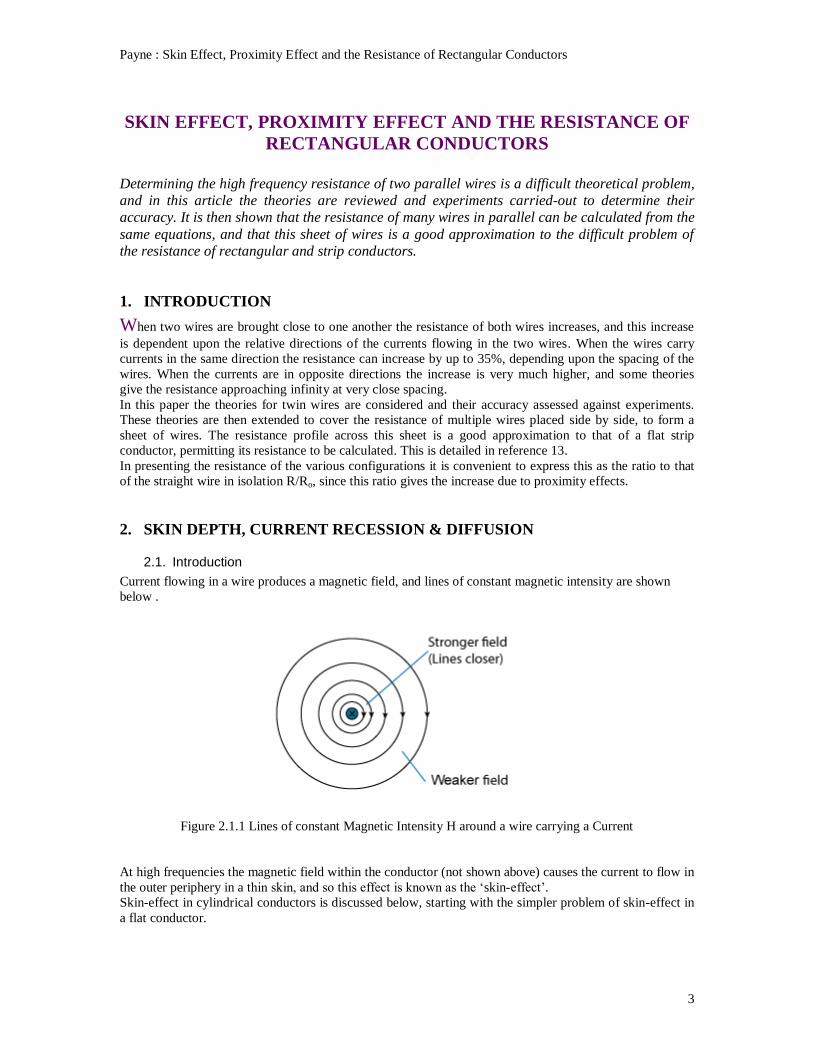
Current flowing in a wire produces a magnetic field, and lines of constant magnetic intensity are shown
below .
Figure 2.1.1 Lines of constant Magnetic Intensity H around a wire carrying a Current
At high frequencies the magnetic field within the conductor (not shown above) causes the current to flow in
the outer periphery in a thin skin, and so this effect is known as the ‘skin-effect’.
Skin-effect in cylindrical conductors is discussed below, starting with the simpler problem of skin-effect in
a flat conductor.
Payne : Skin Effect, Proximity Effect and the Resistance of Rectangular Conductors
4
2.2. Skin Effect in Wide Flat Conductor
In a wide flat conductor, the current which is set-up on the surface diffuses into the surface exponentially
according to the resistivity of the material, its permeability and the frequency. For a current density Jo at the
surface, the density at depth z is given by (see Ramo & Winnery ref 2, p237) :
Jz = Jo e –z/δ
2.2.1
where δ = [ρ/(πfµ)]0.5
µ= µr µo
µr is the material relative permeability
µo = 4π 10-7
ρ = resistivity (ohm-metres)
Figure 2.2.1 Current density at high frequencies
Thus the current density decays exponentially as shown in the above curve, and so the total current is equal
to the area under this curve, integrated from the surface to the material thickness t ie from z = 0 to z = t :
t
Iav = Jm ∫ e –z/δ
dz 2.2.2
0
t
Iav = Jm [- δ e –z/δ
] = Jm [ - δ e –t/δ
- (-δ)]
0
Iav = Jm δ (1- e –t/δ
) 2.2.3
When the conductor thickness is infinite, the exponential function is zero and the average current becomes
Iav = Jm δ1, This has the same area as that of a current uniformly distributed down to depth of δ, and zero at
greater depths and this leads to the definition of skin depth :
Skin depth δ∞ = [ρ/(πfµ)]0.5
2.2.4
Although the skin depth defined above has been calculated assuming an infinite thickness of conductor,
Equation 2.2.3 shows that the current density at two skin depths has dropped to e-2
= 0.14 or to a power of
about 2% of that at the surface. So this suggests that Equation 2.2.4 applies as long as the thickness of the
conductor is greater than two skin depths. However Wheeler (ref 1) says that this is true for a metal screen
where penetration is from one side only, but in a flat conductor penetration is from two sides and then the
thickness must be four skin depths for Equation 2.2.4 to be valid. However an experiment by the author
(Section 6.4.1) does not support Wheeler’s statement (this experiment is in support of Equation 2.2.5
below, but the same arguments would apply). See also Section 2.5.
Payne : Skin Effect, Proximity Effect and the Resistance of Rectangular Conductors
5
0.001
0.010
0.100
1.000
10.000
0.001 0.01 0.1 1 10 100 1000
Sk
in D
ep
th m
m
Frequency MHz
Resistance
Skin Depth in Copper mm
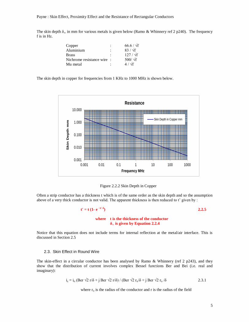
The skin depth δ∞ in mm for various metals is given below (Ramo & Whinnery ref 2 p240). The frequency
f is in Hz.
Copper : 66.6 / √f
Aluminium : 83 / √f
Brass : 127 / √f
Nichrome resistance wire : 500/ √f
Mu metal : 4 / √f
The skin depth in copper for frequencies from 1 KHz to 1000 MHz is shown below.
Figure 2.2.2 Skin Depth in Copper
Often a strip conductor has a thickness t which is of the same order as the skin depth and so the assumption
above of a very thick conductor is not valid. The apparent thickness is then reduced to t’ given by :
t' = t (1- e –t/
δ) 2.2.5
where t is the thickness of the conductor
δ∞ is given by Equation 2.2.4
Notice that this equation does not include terms for internal reflection at the metal/air interface. This is
discussed in Section 2.5
2.3. Skin Effect in Round Wire
The skin-effect in a circular conductor has been analysed by Ramo & Whinnery (ref 2 p243), and they
show that the distribution of current involves complex Bessel functions Ber and Bei (i.e. real and
imaginary):
iz = io (Ber √2 r/δ + j Ber √2 r/δ) / (Ber √2 ro/δ + j Ber √2 ro /δ 2.3.1
where ro is the radius of the conductor and r is the radius of the field
Payne : Skin Effect, Proximity Effect and the Resistance of Rectangular Conductors
6
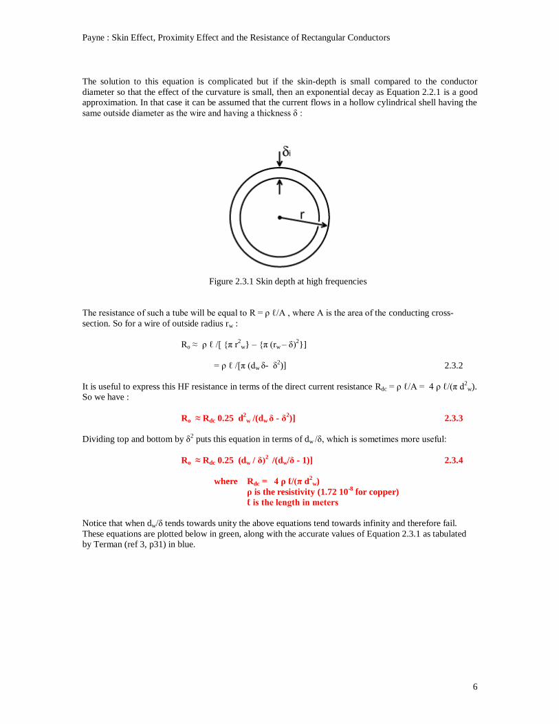
The solution to this equation is complicated but if the skin-depth is small compared to the conductor
diameter so that the effect of the curvature is small, then an exponential decay as Equation 2.2.1 is a good
approximation. In that case it can be assumed that the current flows in a hollow cylindrical shell having the
same outside diameter as the wire and having a thickness δ :
Figure 2.3.1 Skin depth at high frequencies
The resistance of such a tube will be equal to R = ρ ℓ/A , where A is the area of the conducting cross-
section. So for a wire of outside radius rw :
Ro ≈ ρ ℓ /[ {π r2
w} – {π (rw – δ)2}]
= ρ ℓ /[π (dw δ- δ2)] 2.3.2
It is useful to express this HF resistance in terms of the direct current resistance Rdc = ρ ℓ/A = 4 ρ ℓ/(π d2
w).
So we have :
Ro ≈ Rdc 0.25 d2
w /(dw δ - δ2)] 2.3.3
Dividing top and bottom by δ2 puts this equation in terms of dw /δ, which is sometimes more useful:
Ro ≈ Rdc 0.25 (dw / δ)2 /(dw/δ - 1)] 2.3.4
where Rdc = 4 ρ ℓ/(π d2
w)
ρ is the resistivity (1.72 10-8
for copper)
ℓ is the length in meters
Notice that when dw/δ tends towards unity the above equations tend towards infinity and therefore fail.
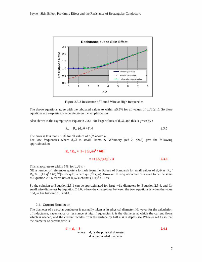
These equations are plotted below in green, along with the accurate values of Equation 2.3.1 as tabulated
by Terman (ref 3, p31) in blue.
Payne : Skin Effect, Proximity Effect and the Resistance of Rectangular Conductors
7
Figure 2.3.2 Resistance of Round Wire at High frequencies
The above equations agree with the tabulated values to within ±5.5% for all values of dw/δ ≥1.6. So these
equations are surprisingly accurate given the simplification.
Also shown is the asymptote of Equation 2.3.1 for large values of dw/δ, and this is given by :
Ro ≈ Rdc (dw/δ +1)/4 2.3.5
The error is less than -1.3% for all values of dw/δ above 4.
For low frequencies where dw/δ is small, Ramo & Whinnery (ref 2, p245) give the following
approximation:
Ro / Rdc ≈ 1+ [ (dw/δ)4 / 768]
= 1+ [dw/(4δ)]4 / 3 2.3.6
This is accurate to within 5% for dw/δ ≤ 4.
NB a number of references quote a formula from the Bureau of Standards for small values of dw/δ as Ro /
Rdc ≈ [ (1+ q4 / 48)
0.5]/2 for q<3, where q= (√2 ro/δ). However this equation can be shown to be the same
as Equation 2.3.6 for values of dw/δ such that (1+x)n ≈ 1+nx.
So the solution to Equation 2.3.1 can be approximated for large wire diameters by Equation 2.3.4, and for
small wire diameters by Equation 2.3.6, where the changeover between the two equations is when the value
of dw/δ lies between 1.6 and 4.
2.4. Current Recession
The diameter of a circular conductor is normally taken as its physical diameter. However for the calculation
of inductance, capacitance or resistance at high frequencies it is the diameter at which the current flows
which is needed, and the current recedes from the surface by half a skin depth (see Wheeler ref 1) so that
the diameter of current flow is :
d' = dw – δ 2.4.1
where dw is the physical diameter
d is the receded diameter
0.0
0.5
1.0
1.5
2.0
2.5
0 1 2 3 4 5 6 7 8
Re
sis
tan
ce
Ra
tio
d/δ
Resistance due to Skin Effect
Rhf/Rdc (Terman)
Rhf/Rdc (asymptote)
Hollow tube approximation
Payne : Skin Effect, Proximity Effect and the Resistance of Rectangular Conductors
8
Where current recession applies the equations are given in terms of d’ rather than dw.
2.5. EM Wave or Diffusion ?
Associated with the exponential reduction in amplitude (Equation 2.2.1) is a change of phase, with an angle
of one radian at one skin depth. The penetration into the conductor thus has a wave-like characteristic and
indeed it is normally described as the penetration of an EM wave into the conductor. However there is an
alternative view, and Spreen (ref 10) shows that Equation 2.2.1 can also describe diffusion, which is
defined as the net movement of a substance from a region of high concentration to a region of low
concentration. Given that conduction in metals is a movement of charged particles (electrons), diffusion
seems to the author to be a more likely mechanism.
Why should this matter if the equations are the same? Imagine a flat plane conductor with an EM wave
starting at one face, traversing the thickness of the conductor and reaching the opposite face. At this surface
there is a major discontinuity with the air, and the wave will be reflected. Given that the wave impedance in
the metal, E/H will be around 1/100th that in the air the situation is akin to a transmission-line terminated in
a very high impedance, so that the forward current at the surface will be nearly cancelled by that of the
return wave. Alternatively if diffusion is the mechanism there will be no reflection and there will be a
significant current at the opposite surface.
One test of the two viewpoints comes from considering the screening effect of a metal sheet, since the
reflection of a wave at the opposite surface would add considerably to the screening effect. Wheeler (ref 1)
assumes a reflection at the interface to air but says that this reduces the screening effect, due to a doubling
of the current at the surface. So presumably he assumes that the ‘transmission-line’ is terminated in a low
impedance at the interface.
To resolve this issue the author has conducted experiments and shown that the penetration is due to
diffusion (ref 12).
3. PROXIMITY LOSS IN TWIN WIRES – CURRENTS IN SAME DIRECTION
3.1. Introduction
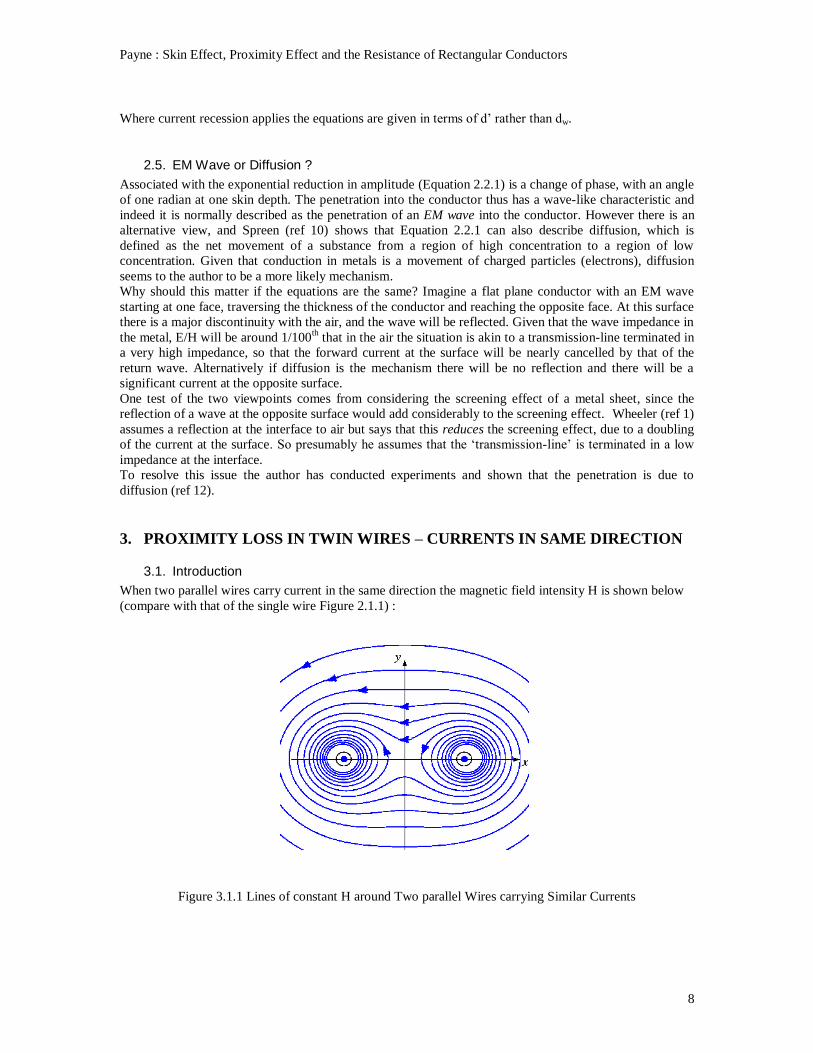
When two parallel wires carry current in the same direction the magnetic field intensity H is shown below
(compare with that of the single wire Figure 2.1.1) :
Figure 3.1.1 Lines of constant H around Two parallel Wires carrying Similar Currents
Payne : Skin Effect, Proximity Effect and the Resistance of Rectangular Conductors
9
1.00
1.05
1.10
1.15
1.20
1.25
1.30
1.35
1.40
1.45
1.0 1.5 2.0 2.5 3.0 3.5 4.0
Re
sis
tan
ce R
ati
o
Conductor Spacing p/d
Proximity Ratio for 2 Wires Currents in same direction
Butterworth 1925 (Table VIII)
Author's Theory
Butterworth 1921
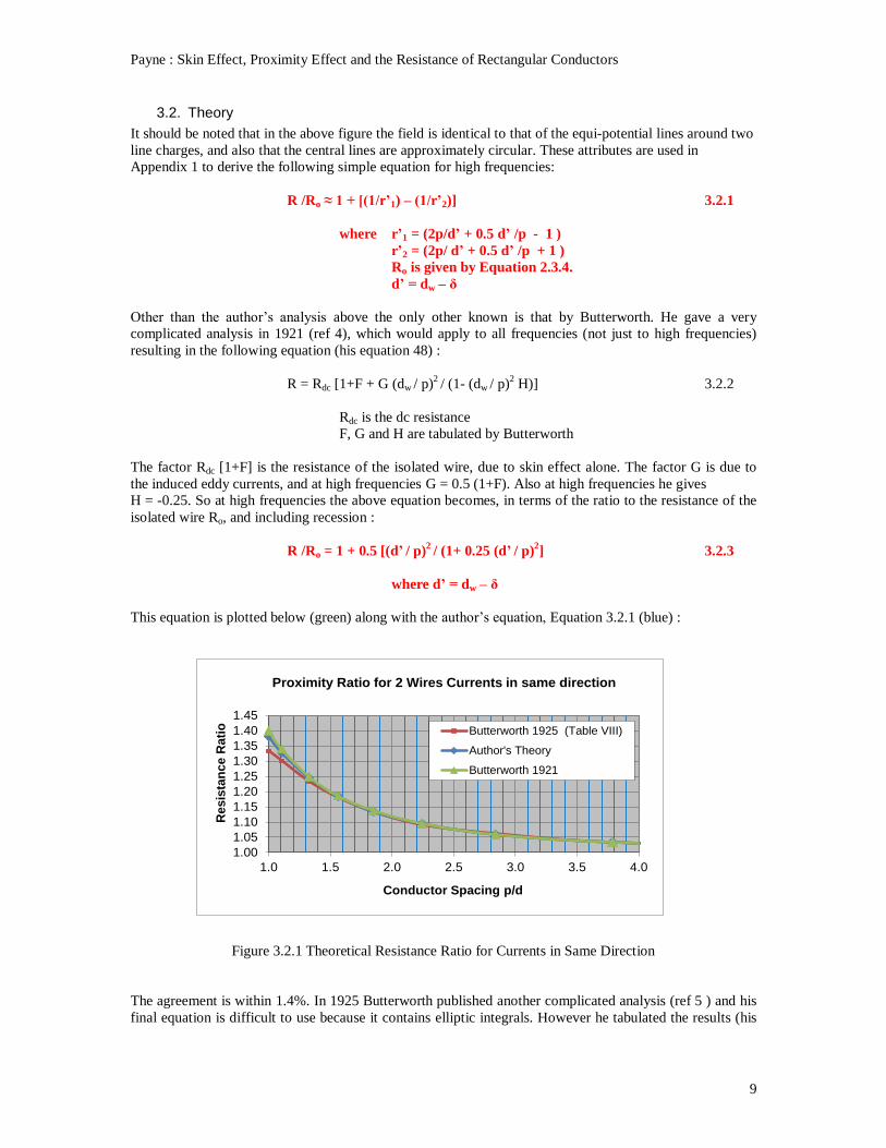
3.2. Theory
It should be noted that in the above figure the field is identical to that of the equi-potential lines around two
line charges, and also that the central lines are approximately circular. These attributes are used in
Appendix 1 to derive the following simple equation for high frequencies:
R /Ro ≈ 1 + [(1/r’1) – (1/r’2)] 3.2.1
where r’1 = (2p/d’ + 0.5 d’ /p - 1 )
r’2 = (2p/ d’ + 0.5 d’ /p + 1 )
Ro is given by Equation 2.3.4.
d’ = dw – δ
Other than the author’s analysis above the only other known is that by Butterworth. He gave a very
complicated analysis in 1921 (ref 4), which would apply to all frequencies (not just to high frequencies)
resulting in the following equation (his equation 48) :
R = Rdc [1+F + G (dw / p)2 / (1- (dw / p)
2 H)] 3.2.2
Rdc is the dc resistance
F, G and H are tabulated by Butterworth
The factor Rdc [1+F] is the resistance of the isolated wire, due to skin effect alone. The factor G is due to
the induced eddy currents, and at high frequencies G = 0.5 (1+F). Also at high frequencies he gives
H = -0.25. So at high frequencies the above equation becomes, in terms of the ratio to the resistance of the
isolated wire Ro, and including recession :
R /Ro = 1 + 0.5 [(d’ / p)2 / (1+ 0.25 (d’ / p)
2] 3.2.3
where d’ = dw – δ
This equation is plotted below (green) along with the author’s equation, Equation 3.2.1 (blue) :
Figure 3.2.1 Theoretical Resistance Ratio for Currents in Same Direction
The agreement is within 1.4%. In 1925 Butterworth published another complicated analysis (ref 5 ) and his
final equation is difficult to use because it contains elliptic integrals. However he tabulated the results (his
Payne : Skin Effect, Proximity Effect and the Resistance of Rectangular Conductors
10
1.0
1.1
1.2
1.3
1.4
1.0 1.1 1.2 1.3 1.4 1.5
Re
sis
tan
ce
R
ati
o
p/dw (receded)
Resistance Ratio same Currents
Measured- Both Ends connected
Theoretical (Butterworth approx)
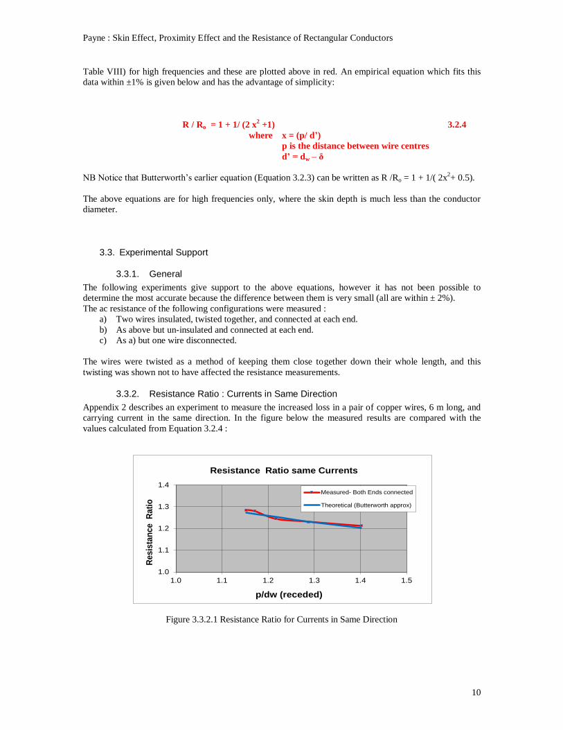
Table VIII) for high frequencies and these are plotted above in red. An empirical equation which fits this
data within ±1% is given below and has the advantage of simplicity:
R / Ro = 1 + 1/ (2 x2 +1) 3.2.4
where x = (p/ d’)
p is the distance between wire centres
d’ = dw – δ
NB Notice that Butterworth’s earlier equation (Equation 3.2.3) can be written as R /Ro = 1 + 1/( 2x2+ 0.5).
The above equations are for high frequencies only, where the skin depth is much less than the conductor
diameter.
3.3. Experimental Support
3.3.1. General
The following experiments give support to the above equations, however it has not been possible to
determine the most accurate because the difference between them is very small (all are within ± 2%).
The ac resistance of the following configurations were measured :
a) Two wires insulated, twisted together, and connected at each end.
b) As above but un-insulated and connected at each end.
c) As a) but one wire disconnected.
The wires were twisted as a method of keeping them close together down their whole length, and this
twisting was shown not to have affected the resistance measurements.
3.3.2. Resistance Ratio : Currents in Same Direction
Appendix 2 describes an experiment to measure the increased loss in a pair of copper wires, 6 m long, and
carrying current in the same direction. In the figure below the measured results are compared with the
values calculated from Equation 3.2.4 :
Figure 3.3.2.1 Resistance Ratio for Currents in Same Direction
Payne : Skin Effect, Proximity Effect and the Resistance of Rectangular Conductors
11
1
2
3
4
5
6
7
8
9
0 2 4 6 8 10 12 14 16
Resis
tan
ce
Oh
ms
Frequency MHz
Measured Proximity Loss
Double wire not insulated x 2
Double wire insulated x 2
One wire of insulated twist
Single Wire
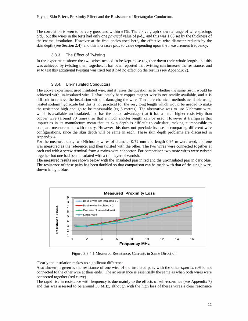
The correlation is seen to be very good and within ±1%. The above graph shows a range of wire spacings
p/dw, but the wires in the tests had only one physical value of p/dw, and this was 1.08 set by the thickness of
the enamel insulation. However at the frequencies used here, the effective wire diameter reduces by the
skin depth (see Section 2.4), and this increases p/dw to value depending upon the measurement frequency.
3.3.3. The Effect of Twisting
In the experiment above the two wires needed to be kept close together down their whole length and this
was achieved by twisting them together. It has been reported that twisting can increase the resistance, and
so to test this additional twisting was tried but it had no effect on the results (see Appendix 2).
3.3.4. Un-insulated Conductors
The above experiment used insulated wire, and it raises the question as to whether the same result would be
achieved with un-insulated wire. Unfortunately bare copper magnet wire is not readily available, and it is
difficult to remove the insulation without damaging the wire. There are chemical methods available using
heated sodium hydroxide but this is not practical for the very long length which would be needed to make
the resistance high enough to be measurable (eg 6 metres). The alternative was to use Nichrome wire,
which is available un-insulated, and has the added advantage that it has a much higher resistivity than
copper wire (around 70 times), so that a much shorter length can be used. However it transpires that
impurities in its manufacture mean that its skin depth is difficult to calculate, making it impossible to
compare measurements with theory. However this does not preclude its use in comparing different wire
configurations, since the skin depth will be same in each. These skin depth problems are discussed in
Appendix 4.
For the measurements, two Nichrome wires of diameter 0.72 mm and length 0.97 m were used, and one
was measured as the reference, and then twisted with the other. The two wires were connected together at
each end with a screw terminal from a mains-wire connector. For comparison two more wires were twisted
together but one had been insulated with a thin layer of varnish.
The measured results are shown below with the insulated pair in red and the un-insulated pair in dark blue.
The resistance of these pairs has been doubled so that comparison can be made with that of the single wire,
shown in light blue.
Figure 3.3.4.1 Measured Resistance: Currents in Same Direction
Clearly the insulation makes no significant difference.
Also shown in green is the resistance of one wire of the insulated pair, with the other open circuit ie not
connected to the other wire at their ends. The ac resistance is essentially the same as when both wires were
connected together (red curve).
The rapid rise in resistance with frequency is due mainly to the effects of self-resonance (see Appendix 7)
and this was assessed to be around 30 MHz, although with the high loss of theses wires a clear resonance
Payne : Skin Effect, Proximity Effect and the Resistance of Rectangular Conductors
12
0.90
1.00
1.10
1.20
1.30
1.40
0.00 0.20 0.40 0.60 0.80
Res
ista
nc
e R
ati
o
Skin Depth/dw
Measured Resistance Ratio
Measured Ratio Double to Single
Linear Approx
was not present. The SRF was therefore very close to the maximum measurement frequency, and a small
difference in the SRF between the configurations probably accounts for the difference between the curves
at high frequencies.
3.3.5. Variation of Resistance with Frequency
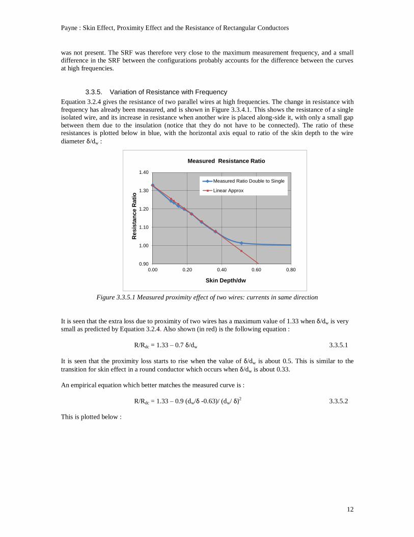
Equation 3.2.4 gives the resistance of two parallel wires at high frequencies. The change in resistance with
frequency has already been measured, and is shown in Figure 3.3.4.1. This shows the resistance of a single
isolated wire, and its increase in resistance when another wire is placed along-side it, with only a small gap
between them due to the insulation (notice that they do not have to be connected). The ratio of these
resistances is plotted below in blue, with the horizontal axis equal to ratio of the skin depth to the wire
diameter δ/dw :
Figure 3.3.5.1 Measured proximity effect of two wires: currents in same direction
It is seen that the extra loss due to proximity of two wires has a maximum value of 1.33 when δ/dw is very
small as predicted by Equation 3.2.4. Also shown (in red) is the following equation :
R/Rdc = 1.33 – 0.7 δ/dw 3.3.5.1
It is seen that the proximity loss starts to rise when the value of δ/dw is about 0.5. This is similar to the
transition for skin effect in a round conductor which occurs when δ/dw is about 0.33.
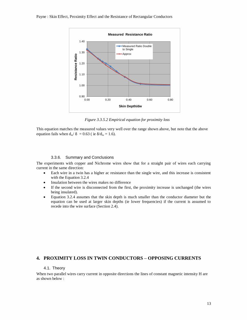
An empirical equation which better matches the measured curve is :
R/Rdc = 1.33 – 0.9 (dw/δ -0.63)/ (dw/ δ)2 3.3.5.2
This is plotted below :
Payne : Skin Effect, Proximity Effect and the Resistance of Rectangular Conductors
13
0.90
1.00
1.10
1.20
1.30
1.40
0.00 0.20 0.40 0.60 0.80
Res
ista
nc
e R
ati
o
Skin Depth/dw
Measured Resistance Ratio
Measured Ratio Doubleto Single
Approx
Figure 3.3.5.2 Empirical equation for proximity loss
This equation matches the measured values very well over the range shown above, but note that the above
equation fails when dw/ δ = 0.63 ( ie δ/dw = 1.6).
3.3.6. Summary and Conclusions
The experiments with copper and Nichrome wires show that for a straight pair of wires each carrying
current in the same direction:
Each wire in a twin has a higher ac resistance than the single wire, and this increase is consistent
with the Equation 3.2.4
Insulation between the wires makes no difference
If the second wire is disconnected from the first, the proximity increase is unchanged (the wires
being insulated).
Equation 3.2.4 assumes that the skin depth is much smaller than the conductor diameter but the
equation can be used at larger skin depths (ie lower frequencies) if the current is assumed to
recede into the wire surface (Section 2.4).
4. PROXIMITY LOSS IN TWIN CONDUCTORS – OPPOSING CURRENTS
4.1. Theory
When two parallel wires carry current in opposite directions the lines of constant magnetic intensity H are
as shown below :
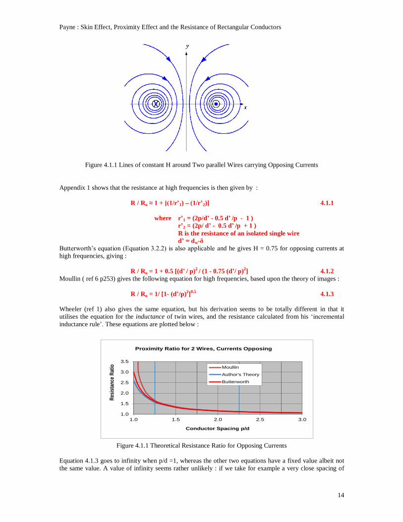
Payne : Skin Effect, Proximity Effect and the Resistance of Rectangular Conductors
14
1.0
1.5
2.0
2.5
3.0
3.5
1.0 1.5 2.0 2.5 3.0
Res
ista
nce
Rat
io
Conductor Spacing p/d
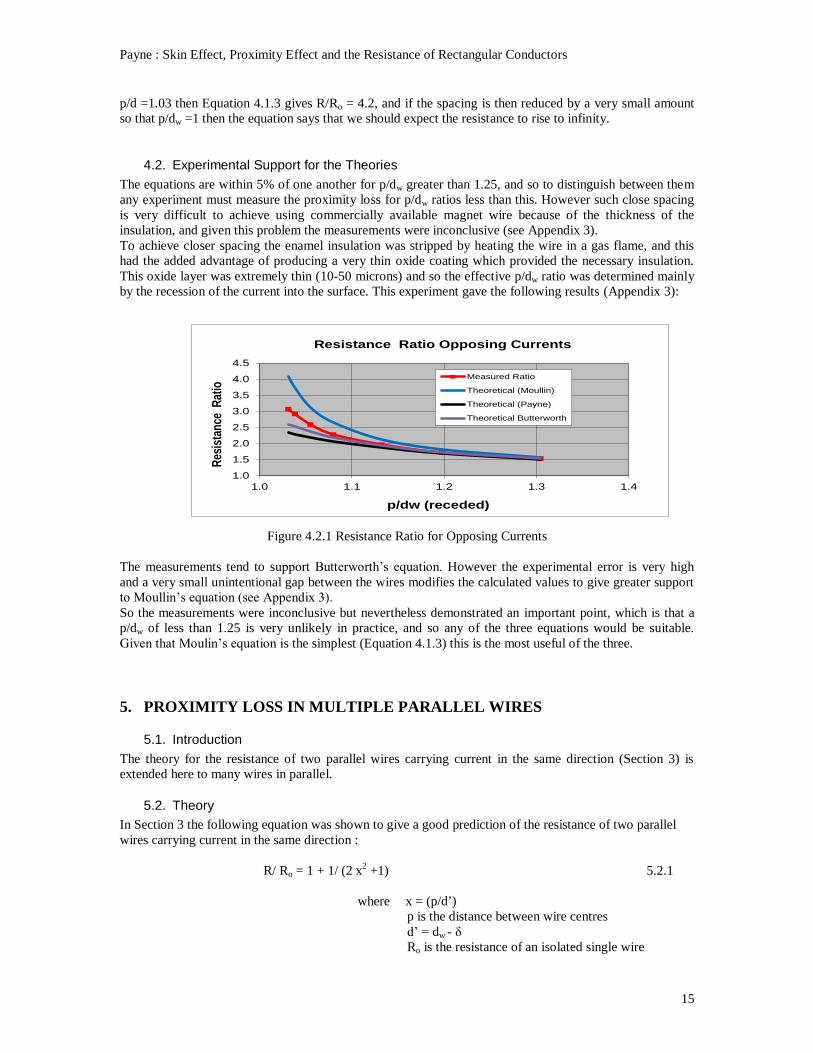
Proximity Ratio for 2 Wires, Currents Opposing
Moullin
Author's Theory
Butterworth
Figure 4.1.1 Lines of constant H around Two parallel Wires carrying Opposing Currents
Appendix 1 shows that the resistance at high frequencies is then given by :
R / Ro ≈ 1 + [(1/r’1) – (1/r’2)] 4.1.1
where r’1 = (2p/d’ - 0.5 d’ /p - 1 )
r’2 = (2p/ d’ - 0.5 d’ /p + 1 )
R is the resistance of an isolated single wire
d’ = dw-δ
Butterworth’s equation (Equation 3.2.2) is also applicable and he gives H = 0.75 for opposing currents at
high frequencies, giving :
R / Ro = 1 + 0.5 [(d’ / p)2 / (1 - 0.75 (d’/ p)
2] 4.1.2
Moullin ( ref 6 p253) gives the following equation for high frequencies, based upon the theory of images :
R / Ro = 1/ [1- (d’/p)2]
0.5 4.1.3
Wheeler (ref 1) also gives the same equation, but his derivation seems to be totally different in that it
utilises the equation for the inductance of twin wires, and the resistance calculated from his ‘incremental
inductance rule’. These equations are plotted below :
Figure 4.1.1 Theoretical Resistance Ratio for Opposing Currents
Equation 4.1.3 goes to infinity when p/d =1, whereas the other two equations have a fixed value albeit not
the same value. A value of infinity seems rather unlikely : if we take for example a very close spacing of
Payne : Skin Effect, Proximity Effect and the Resistance of Rectangular Conductors
15
1.0
1.5
2.0
2.5
3.0
3.5
4.0
4.5
1.0 1.1 1.2 1.3 1.4
Res
ista
nce
Rat
io
p/dw (receded)
Resistance Ratio Opposing Currents
Measured Ratio
Theoretical (Moullin)
Theoretical (Payne)
Theoretical Butterworth
p/d =1.03 then Equation 4.1.3 gives R/Ro = 4.2, and if the spacing is then reduced by a very small amount
so that p/dw =1 then the equation says that we should expect the resistance to rise to infinity.
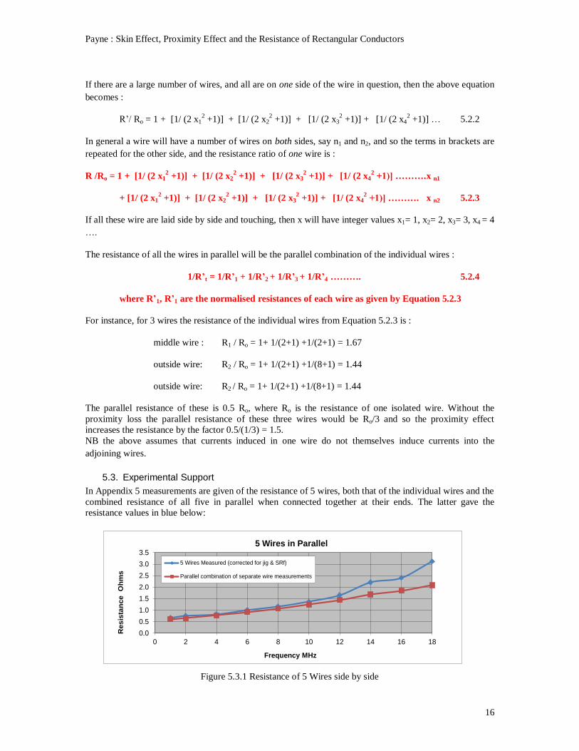
4.2. Experimental Support for the Theories
The equations are within 5% of one another for p/dw greater than 1.25, and so to distinguish between them
any experiment must measure the proximity loss for p/dw ratios less than this. However such close spacing
is very difficult to achieve using commercially available magnet wire because of the thickness of the
insulation, and given this problem the measurements were inconclusive (see Appendix 3).
To achieve closer spacing the enamel insulation was stripped by heating the wire in a gas flame, and this
had the added advantage of producing a very thin oxide coating which provided the necessary insulation.
This oxide layer was extremely thin (10-50 microns) and so the effective p/dw ratio was determined mainly
by the recession of the current into the surface. This experiment gave the following results (Appendix 3):
Figure 4.2.1 Resistance Ratio for Opposing Currents
The measurements tend to support Butterworth’s equation. However the experimental error is very high
and a very small unintentional gap between the wires modifies the calculated values to give greater support
to Moullin’s equation (see Appendix 3).
So the measurements were inconclusive but nevertheless demonstrated an important point, which is that a
p/dw of less than 1.25 is very unlikely in practice, and so any of the three equations would be suitable.
Given that Moulin’s equation is the simplest (Equation 4.1.3) this is the most useful of the three.
5. PROXIMITY LOSS IN MULTIPLE PARALLEL WIRES
5.1. Introduction
The theory for the resistance of two parallel wires carrying current in the same direction (Section 3) is
extended here to many wires in parallel.
5.2. Theory
In Section 3 the following equation was shown to give a good prediction of the resistance of two parallel
wires carrying current in the same direction :
R/ Ro = 1 + 1/ (2 x2 +1) 5.2.1
where x = (p/d’)
p is the distance between wire centres
d’ = dw - δ
Ro is the resistance of an isolated single wire
Payne : Skin Effect, Proximity Effect and the Resistance of Rectangular Conductors
16
0.0
0.5
1.0
1.5
2.0
2.5
3.0
3.5
0 2 4 6 8 10 12 14 16 18
Re
sis
tan
ce
Oh
ms
Frequency MHz
5 Wires in Parallel
5 Wires Measured (corrected for jig & SRf)
Parallel combination of separate wire measurements
If there are a large number of wires, and all are on one side of the wire in question, then the above equation
becomes :
R’/ Ro = 1 + [1/ (2 x12 +1)] + [1/ (2 x2
2 +1)] + [1/ (2 x3
2 +1)] + [1/ (2 x4
2 +1)] … 5.2.2
In general a wire will have a number of wires on both sides, say n1 and n2, and so the terms in brackets are
repeated for the other side, and the resistance ratio of one wire is :
R /Ro = 1 + [1/ (2 x12 +1)] + [1/ (2 x2
2 +1)] + [1/ (2 x3
2 +1)] + [1/ (2 x4
2 +1)] ………. x n1
+ [1/ (2 x12 +1)] + [1/ (2 x2
2 +1)] + [1/ (2 x3
2 +1)] + [1/ (2 x4
2 +1)] ………. x n2 5.2.3
If all these wire are laid side by side and touching, then x will have integer values x1= 1, x2= 2, x3= 3, x4 = 4
….
The resistance of all the wires in parallel will be the parallel combination of the individual wires :
1/R’t = 1/R’1 + 1/R’2 + 1/R’3 + 1/R’4 ………. 5.2.4
where R’1, R’1 are the normalised resistances of each wire as given by Equation 5.2.3
For instance, for 3 wires the resistance of the individual wires from Equation 5.2.3 is :
middle wire : R1 / Ro = 1+ 1/(2+1) +1/(2+1) = 1.67
outside wire: R2 / Ro = 1+ 1/(2+1) +1/(8+1) = 1.44
outside wire: R2 / Ro = 1+ 1/(2+1) +1/(8+1) = 1.44
The parallel resistance of these is 0.5 Ro, where Ro is the resistance of one isolated wire. Without the
proximity loss the parallel resistance of these three wires would be Ro/3 and so the proximity effect
increases the resistance by the factor 0.5/(1/3) = 1.5.
NB the above assumes that currents induced in one wire do not themselves induce currents into the
adjoining wires.
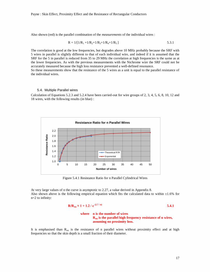
5.3. Experimental Support
In Appendix 5 measurements are given of the resistance of 5 wires, both that of the individual wires and the
combined resistance of all five in parallel when connected together at their ends. The latter gave the
resistance values in blue below:
Figure 5.3.1 Resistance of 5 Wires side by side
Payne : Skin Effect, Proximity Effect and the Resistance of Rectangular Conductors
17
1.0
1.2
1.4
1.6
1.8
2.0
2.2
0 5 10 15 20 25 30 35 40 45 50
Resis
tan
ce R
ati
o
Number of wires
Resistance Ratio for n Parallel Wires
Theoretical R'/R
Exponential
Also shown (red) is the parallel combination of the measurements of the individual wires :
R = 1/[1/R1 +1/R2+1/R3+1/R4+1/R5 ] 5.3.1
The correlation is good at the low frequencies, but degrades above 10 MHz probably because the SRF with
5 wires in parallel is slightly different to that of each individual wire, and indeed if it is assumed that the
SRF for the 5 in parallel is reduced from 35 to 29 MHz the correlation at high frequencies is the same as at
the lower frequencies. As with the previous measurements with the Nichrome wire the SRF could not be
accurately measured because the high loss resistance prevented a well-defined resonance.
So these measurements show that the resistance of the 5 wires as a unit is equal to the parallel resistance of
the individual wires.
5.4. Multiple Parallel wires
Calculation of Equations 5.2.3 and 5.2.4 have been carried-out for wire groups of 2, 3, 4, 5, 6, 8, 10, 12 and
18 wires, with the following results (in blue) :
Figure 5.4.1 Resistance Ratio for n Parallel Cylindrical Wires
At very large values of n the curve is asymptotic to 2.27, a value derived in Appendix 8.
Also shown above is the following empirical equation which fits the calculated data to within ±1.6% for
n=2 to infinity:
R/Ron ≈ 1 + 1.2 / e (2.7 / n)
5.4.1
where n is the number of wires
Ron is the parallel high frequency resistance of n wires,
assuming no proximity loss.
It is emphasised than Ron is the resistance of n parallel wires without proximity effect and at high
frequencies so that the skin depth is a small fraction of their diameter.
Payne : Skin Effect, Proximity Effect and the Resistance of Rectangular Conductors
18
6. RESISTANCE OF A CONDUCTOR WITH A RECTANGULAR CROSS-
SECTION
The author’s work on rectangular conductors expanded considerably after issue 2 of this report, to the
extent that it justified a separate document. This is given in reference 13.
7. SUMMARY OF EQUATIONS
The resistance of a single isolated circular wire is given by the following equation for dw/δ > 1.6 :
Ro ≈ Rdc 0.25 (dw / δ)2 /(dw/δ - 1)] 7.1.1
where Rdc = ρ ℓ /A
A is the cross sectional area = π (dw/2)2
dw is the wire diameter
δ = [ρ/(πfµ)]0.5
µ= µr µo
µr is the material relative permeability
µo = 4π 10-7
ρ = resistivity (ohm-metres)
The resistance of a pair of circular wires with currents in the same direction is given by :
R ≈ Ro [1 + 1/ (2 x2 +1)] 7.1.2
where x = (p/d’)
p is the distance between wire centres
d’ is the receded diameter of the wire = dw- δ
Ro is given by Equation 7.1.1
The resistance of a pair of circular wires with currents in opposite directions is given by :
R ≈ Ro / [1- (d’/p)2]0.5
7.1.3
The resistance of a n circular wires, insulated or un-insulated, laid side-by-side and connected together at
each end is given by :
R/Ron ≈ 1 + 1.2 / e (2.7 / n)
7.1.4
where n is the number of wires
Ron is the parallel high frequency resistance of n wires,
assuming no proximity loss.
Payne : Skin Effect, Proximity Effect and the Resistance of Rectangular Conductors
19
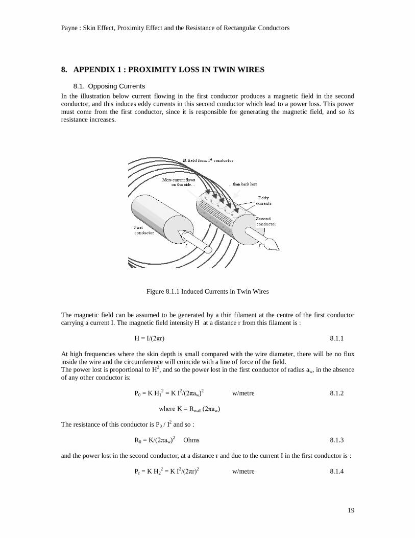
8. APPENDIX 1 : PROXIMITY LOSS IN TWIN WIRES
8.1. Opposing Currents
In the illustration below current flowing in the first conductor produces a magnetic field in the second
conductor, and this induces eddy currents in this second conductor which lead to a power loss. This power
must come from the first conductor, since it is responsible for generating the magnetic field, and so its
resistance increases.
Figure 8.1.1 Induced Currents in Twin Wires
The magnetic field can be assumed to be generated by a thin filament at the centre of the first conductor
carrying a current I. The magnetic field intensity H at a distance r from this filament is :
H = I/(2πr) 8.1.1
At high frequencies where the skin depth is small compared with the wire diameter, there will be no flux
inside the wire and the circumference will coincide with a line of force of the field.
The power lost is proportional to H2, and so the power lost in the first conductor of radius aw, in the absence
of any other conductor is:
P0 = K H12 = K I
2/(2πaw)
2 w/metre 8.1.2
where K = Rwall (2πaw)
The resistance of this conductor is P0 / I2 and so :
R0 = K/(2πaw)2 Ohms 8.1.3
and the power lost in the second conductor, at a distance r and due to the current I in the first conductor is :
Pr = K H22 = K I
2/(2πr)
2 w/metre 8.1.4
Payne : Skin Effect, Proximity Effect and the Resistance of Rectangular Conductors
20
Since this power must come from the first conductor its resistance increases by :
R2 = K/(2πr)2 8.1.5
So the increase in resistance, as a ratio of the resistance of the first conductor is:
R2/ R0 = (aw/r)2 = (1/r’)
2 8.1.6
Where r’ is r normalised to aw
Integrating over the distance to the second conductor, gives :
r2 r2
R2/ R0 = ∫ (1/ r’)2 dr’ = [(1/r’1) – (1/r’2)] 8.1.7
r1 r1
The total resistance is therefore :
R/Ro = 1 + [(1/r’1) – (1/r’2)] 8.1.8
The limits r’1 and r’2 are the distances to the nearest edge of the second conductor and to its farthest edge,
measured from the centre of the first conductor, and so r’1 = (p/aw -1 ) and r’2 = (p/aw +1 ), when
normalised to aw. These are more conveniently expressed as r’1 = (2 p/dw -1 ) and r’2 = (2p/dw +1 ).
In the analysis above the magnetic field was assumed to be generated by a thin filament at the centre of the
first conductor but the effect of the current in the adjacent conductor is to move this filament off-centre,
towards the adjacent conductor. The limits of integration r’1 and r’2 are therefore reduced, and by an
amount depending upon the proximity of the second conductor, p/dw. For high frequencies where the skin
depth is small compared with the wire diameter, Moullin states (ref 6 page 169-170) ‘the centres of the
lines of force will move from the centres of the wires to the mutually inverse points for both wires’.
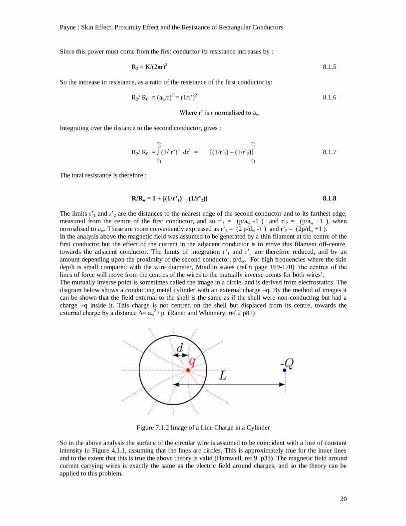
The mutually inverse point is sometimes called the image in a circle, and is derived from electrostatics. The
diagram below shows a conducting metal cylinder with an external charge –q. By the method of images it
can be shown that the field external to the shell is the same as if the shell were non-conducting but had a
charge +q inside it. This charge is not centred on the shell but displaced from its centre, towards the
external charge by a distance Δ= aw2 / p (Ramo and Whinnery, ref 2 p81)
Figure 7.1.2 Image of a Line Charge in a Cylinder
So in the above analysis the surface of the circular wire is assumed to be coincident with a line of constant
intensity in Figure 4.1.1, assuming that the lines are circles. This is approximately true for the inner lines
and to the extent that this is true the above theory is valid (Harnwell, ref 9 p33). The magnetic field around
current carrying wires is exactly the same as the electric field around charges, and so the theory can be
applied to this problem.
Payne : Skin Effect, Proximity Effect and the Resistance of Rectangular Conductors
21
Since we are normalising all dimensions to aw this displacement from the centre becomes Δ’= aw / p = 0.5
dw /p, and Equation 3.2.8 becomes for opposing currents :
R/ Ro ≈ 1 + [(1/r’1) – (1/r’2)] 8.1.9
where r’1 = (2p/dw - 0.5 dw /p - 1 )
r’2 = (2p/dw - 0.5 dw /p + 1 )
8.2. Currents in Same Direction
In Figure 8.1.1 the currents are shown in opposite directions, and the current density is higher on the inner
surface of each conductor, but when currents are in the same direction the current density is higher on the
outer surface. The image therefore moves out from the centre and Equation 8.1.9 becomes :
R/ Ro ≈ 1 + [(1/r’1) – (1/r’2)] 8.1.10
where r’1 = (2p/dw + 0.5 dw /p - 1 )
r’2 = (2p/dw + 0.5 dw /p + 1 )
NB recession of the current is not included in the above equations, but has been included in Equations 3.2.1
and 4.1.1
9. APPENDIX 2 : RESISTANCE MEASUREMENTS, CURRENTS IN SAME
DIRECTION
9.1. Experimental Issues
For the measurement of the resistance of wires with currents in the same direction copper magnet wire
would be very suitable because its purity is well controlled. However its low resistance causes
measurement problems, as given below.
If the tests are to extend to high frequencies (since the equations are for high frequencies) then the SRF
(Appendix 7) must be sufficiently above the maximum measurement frequency. Also the wire diameter
must be large compared with the skin depth at the measurement frequencies. Together these imply a wire
with a short length and a large diameter, but then the resistance will be very low and this cannot be
measured with sufficient accuracy. The resistance could be increased by using a smaller diameter wire, but
then the measurement frequency would have to increase to maintain the skin depth ratio. The wire length
would then have to be reduced to increase the SRF, negating the advantage of the thinner wire. Another
disadvantage of thin wire is that it has a higher thickness of insulation in proportion to its diameter,
preventing close spacing of the wires.
Overall there is a compromise to be made and it was decided to use 4 mm diameter copper wire, with a
length of 6 m. The SRF when folded back on itself (Appendix 7) was around 17 MHz and so measurements
were made from 0.5 to 6 MHz. The lowest frequency is determined by the skin depth, which needs to be
small compared with the wire diameter (25% of the wire dia, at 0.5 MHz), and also by the measurement
errors, which will increase because of the low resistance at low frequencies. The highest frequency is
determined by the increase in resistance due to the SRF (a factor of 1.3 at 6 MHz) and the errors in
correcting for this, although in compensation the higher resistance at high frequencies reduces the
measurement error.
Two measurements were made, firstly of the ac resistance of a single wire and then of two wires arranged
side by side. This was achieved by twisting the two together, with 200 turns, and then giving the whole
length a slight stretch to mimimise untwisting when the tension was removed. The two wires were soldered
together at each end, the resistance measured and compared with that of the single wire. To minimise the
SRF the single wire was folded-back on itself with spacing of only around 30 mm, and the same was done
Payne : Skin Effect, Proximity Effect and the Resistance of Rectangular Conductors
22
1.0
1.1
1.2
1.3
1.4
1.0 1.1 1.2 1.3 1.4 1.5
Re
sis
tan
ce
R
ati
o
p/dw (receded)
Resistance Ratio same Currents
Measured- Both Ends connected
Theoretical (Butterworth approx)
with the twisted pair. It was hoped that the SRF would be the same, since then no correction would need to
be made for the SRF, but it was found that they gave 16.7 and 18.1 MHz respectively (measured as the
frequency where the phase of Zin went through zeo), giving a correction of 1.32 and 1.26 respectively at 6
MHz. Despite the long length of wire the resistance values were low, ranging from 0.8 to 2.9 Ω for the
twisted pair, and given that the objective was to measure a change of around 20% this equals a change of
only 160 mΩ. If this is to be measured to say 10 % the measurement error must be less than 16 mΩ, and
this required careful calibration. In particular it was important that changes in the resistance of the
connectors used to interface the wire to the VNA were eliminated because contact resistance at each
interface is around 4 mΩ for the SMA connectors used. It was therefore not possible to use the normal
calibration procedure of a short-circuit by replacing the wire and its connector with an SMA short circuit.
Instead with the wire soldered to the connector and this connected to the VNA a short-circuit was placed
across the wire and the measured resistance subtracted for the subsequent measurements, and these need to
be done immediately afterwards to avoid errors due to temperature changes. This ‘zero resistance’
measurement had to be repeated whenever the wire or the connectors were changed, since this
measurement could change as much as 30 mΩ.
In principle the measurement of the twisted pair could be made with only one wire connected to the
measurement equipment and the other left free, and this would have the advantage that the resistance values
would be double that when both wires were connected. This was tried initially but it was found that, in
addition to the expected SRF, there was a low Q resonance at a lower frequency. The cause of this was not
investigated but it is likely to be due to a transmission-line mode between the two wires, whose phase
velocity was slowed by the enamel insulation.
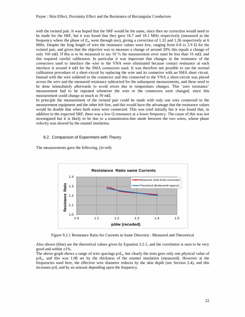
9.2. Comparison of Experiment with Theory
The measurements gave the following, (in red):
Figure 9.2.1 Resistance Ratio for Currents in Same Direction : Measured and Theoretical
Also shown (blue) are the theoretical values given by Equation 3.2.1, and the correlation is seen to be very
good and within ±1%.
The above graph shows a range of wire spacings p/dw, but clearly the tests gave only one physical value of
p/dw, and this was 1.08 set by the thickness of the enamel insulation (measured). However at the
frequencies used here, the effective wire diameter reduces by the skin depth (see Section 2.4), and this
increases p/d, and by an amount depending upon the frequency.
Payne : Skin Effect, Proximity Effect and the Resistance of Rectangular Conductors
23
0.00.10.20.30.40.50.60.70.80.91.01.1
0 2 4 6 8 10 12 14
Resis
tan
ce R
ati
o
Wire Dia/ Skin depth
Resistance Ratio for 2 twists
Ratio of 10mm lay to 30 mmlay
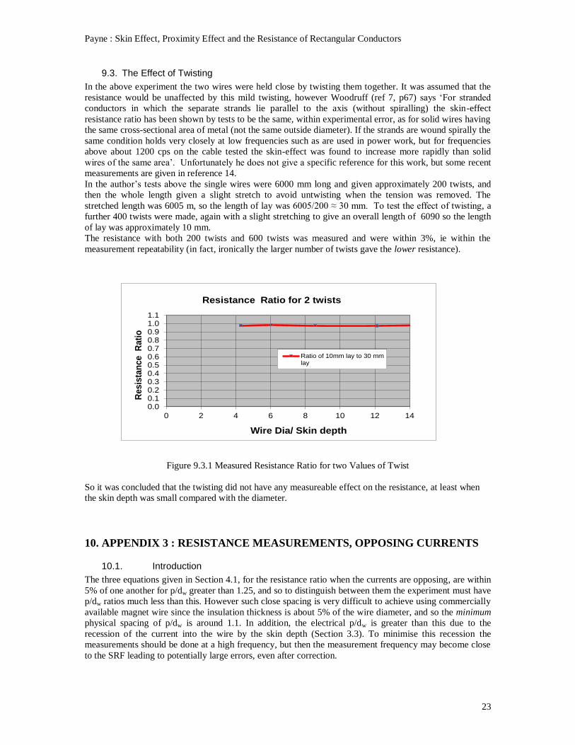
9.3. The Effect of Twisting
In the above experiment the two wires were held close by twisting them together. It was assumed that the
resistance would be unaffected by this mild twisting, however Woodruff (ref 7, p67) says ‘For stranded
conductors in which the separate strands lie parallel to the axis (without spiralling) the skin-effect
resistance ratio has been shown by tests to be the same, within experimental error, as for solid wires having
the same cross-sectional area of metal (not the same outside diameter). If the strands are wound spirally the
same condition holds very closely at low frequencies such as are used in power work, but for frequencies
above about 1200 cps on the cable tested the skin-effect was found to increase more rapidly than solid
wires of the same area’. Unfortunately he does not give a specific reference for this work, but some recent
measurements are given in reference 14.
In the author’s tests above the single wires were 6000 mm long and given approximately 200 twists, and
then the whole length given a slight stretch to avoid untwisting when the tension was removed. The
stretched length was 6005 m, so the length of lay was 6005/200 ≈ 30 mm. To test the effect of twisting, a
further 400 twists were made, again with a slight stretching to give an overall length of 6090 so the length
of lay was approximately 10 mm.
The resistance with both 200 twists and 600 twists was measured and were within 3%, ie within the
measurement repeatability (in fact, ironically the larger number of twists gave the lower resistance).
Figure 9.3.1 Measured Resistance Ratio for two Values of Twist
So it was concluded that the twisting did not have any measureable effect on the resistance, at least when
the skin depth was small compared with the diameter.
10. APPENDIX 3 : RESISTANCE MEASUREMENTS, OPPOSING CURRENTS
10.1. Introduction
The three equations given in Section 4.1, for the resistance ratio when the currents are opposing, are within
5% of one another for p/dw greater than 1.25, and so to distinguish between them the experiment must have
p/dw ratios much less than this. However such close spacing is very difficult to achieve using commercially
available magnet wire since the insulation thickness is about 5% of the wire diameter, and so the minimum
physical spacing of p/dw is around 1.1. In addition, the electrical p/dw is greater than this due to the
recession of the current into the wire by the skin depth (Section 3.3). To minimise this recession the
measurements should be done at a high frequency, but then the measurement frequency may become close
to the SRF leading to potentially large errors, even after correction.
Payne : Skin Effect, Proximity Effect and the Resistance of Rectangular Conductors
24
1.0
1.2
1.4
1.6
1.8
2.0
2.2
1.0 1.1 1.2 1.3 1.4 1.5
Resis
tan
ce R
ati
o
p/dw (receded)
Resistance Ratio Opposing Currents
Measured Ratio
Theoretical (Moullin)
Theoretical (Payne)
Two experiments were carried out, one using conventional insulated magnet wire (accepting the limitation
caused by the thickness of the insulation), and the second using wire which had been stripped of its
insulation in order to reduce the wire spacing. These are described below.
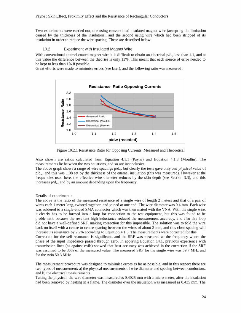
10.2. Experiment with Insulated Magnet Wire
With conventional enamel coated magnet wire it is difficult to obtain an electrical p/dw less than 1.1, and at
this value the difference between the theories is only 13%. This meant that each source of error needed to
be kept to less than 1% if possible.
Great efforts were made to minimise errors (see later), and the following ratio was measured :
Figure 10.2.1 Resistance Ratio for Opposing Currents, Measured and Theoretical
Also shown are ratios calculated from Equation 4.1.1 (Payne) and Equation 4.1.3 (Moullin). The
measurements lie between the two equations, and so are inconclusive.
The above graph shows a range of wire spacings p/dw, but clearly the tests gave only one physical value of
p/dw, and this was 1.08 set by the thickness of the enamel insulation (this was measured). However at the
frequencies used here, the effective wire diameter reduces by the skin depth (see Section 3.3), and this
increases p/dw, and by an amount depending upon the frequency.
Details of experiment :
The above is the ratio of the measured resistance of a single wire of length 2 meters and that of a pair of
wires each 1 meter long, twisted together, and joined at one end. The wire diameter was 0.4 mm. Each wire
was soldered to a single-ended SMA connector which was then mated with the VNA. With the single wire,
it clearly has to be formed into a loop for connection to the test equipment, but this was found to be
problematic because the resultant high inductance reduced the measurement accuracy, and also this loop
did not have a well-defined SRF, making correction for this impossible. The solution was to fold the wire
back on itself with a centre to centre spacing between the wires of about 2 mm, and this close spacing will
increase its resistance by 2.2% according to Equation 4.1.3. The measurements were corrected for this.
Correction for the self-resonance is significant, and the SRF was measured as the frequency where the
phase of the input impedance passed through zero. In applying Equation 14.1, previous experience with
transmission lines (as against coils) showed that best accuracy was achieved in the correction if the SRF
was assumed to be 85% of the measured value. The measured SRF for the single wire was 59.7 MHz and
for the twin 50.3 MHz.
The measurement procedure was designed to minimise errors as far as possible, and in this respect there are
two types of measurement: a) the physical measurements of wire diameter and spacing between conductors,
and b) the electrical measurements.
Taking the physical, the wire diameter was measured as 0.4025 mm with a micro-meter, after the insulation
had been removed by heating in a flame. The diameter over the insulation was measured as 0.435 mm. The
Payne : Skin Effect, Proximity Effect and the Resistance of Rectangular Conductors
25
1.0
1.5
2.0
2.5
3.0
3.5
1.0 1.1 1.2 1.3 1.4
Resis
tan
ce R
ati
o
p/dw (receded)
Resistance Ratio Opposing Currents
Measured Ratio
Theoretical (Moullin)
Theoretical (Payne)
Theoretical Butterworth
wires were twisted together and stretched slightly to prevent the twists unwinding. It was assumed that the
physical spacing was equal to the thickness of the insulation, however there could have been some gaps
which would have increased the spacing between the wires. Alternatively the stretching could have
deformed the wire diameter, thereby reducing the spacing.
The resistance values to be measured are between 0.5 and 3.5 Ω and the contact resistance in the (SMA)
connectors to the VNA was found to be significant, and to reduce the errors here the connectors were
tightened with a spanner. Also the short circuit calibration procedure was as described in Appendix 2.
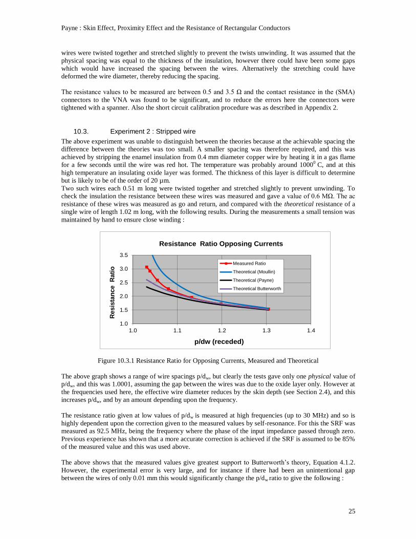
10.3. Experiment 2 : Stripped wire
The above experiment was unable to distinguish between the theories because at the achievable spacing the
difference between the theories was too small. A smaller spacing was therefore required, and this was
achieved by stripping the enamel insulation from 0.4 mm diameter copper wire by heating it in a gas flame
for a few seconds until the wire was red hot. The temperature was probably around 10000
C, and at this
high temperature an insulating oxide layer was formed. The thickness of this layer is difficult to determine
but is likely to be of the order of 20 µm.
Two such wires each 0.51 m long were twisted together and stretched slightly to prevent unwinding. To
check the insulation the resistance between these wires was measured and gave a value of 0.6 MΩ. The ac
resistance of these wires was measured as go and return, and compared with the theoretical resistance of a
single wire of length 1.02 m long, with the following results. During the measurements a small tension was
maintained by hand to ensure close winding :
Figure 10.3.1 Resistance Ratio for Opposing Currents, Measured and Theoretical
The above graph shows a range of wire spacings p/dw, but clearly the tests gave only one physical value of
p/dw, and this was 1.0001, assuming the gap between the wires was due to the oxide layer only. However at
the frequencies used here, the effective wire diameter reduces by the skin depth (see Section 2.4), and this
increases p/dw, and by an amount depending upon the frequency.
The resistance ratio given at low values of p/dw is measured at high frequencies (up to 30 MHz) and so is
highly dependent upon the correction given to the measured values by self-resonance. For this the SRF was
measured as 92.5 MHz, being the frequency where the phase of the input impedance passed through zero.
Previous experience has shown that a more accurate correction is achieved if the SRF is assumed to be 85%
of the measured value and this was used above.
The above shows that the measured values give greatest support to Butterworth’s theory, Equation 4.1.2.
However, the experimental error is very large, and for instance if there had been an unintentional gap
between the wires of only 0.01 mm this would significantly change the p/dw ratio to give the following :
Payne : Skin Effect, Proximity Effect and the Resistance of Rectangular Conductors
26
0.0
0.2
0.4
0.6
0.8
1.0
0 5 10 15 20 25 30
Resis
tan
ce
Oh
ms
Frequency MHz
Resistance
Calculated Resistance single wire inc SRF
Single Wire Measured (corrected)
Figure 10.3.2 Resistance Ratio for Opposing Currents, Measured and Theoretical
This gives greater support to the Moullin equation especially since close examination showed some
evidence of a very small gap in some parts of the winding.
One aspect not considered above is displacement current, due to the capacitance between wires and this
was measured at 120 pf, giving a reactance at 30 MHz (the highest measurement frequency) of –j42 Ω.
However the correction due to the SRF already accounts for the distributed L and C so no further correction
is needed. Welsby’s equation for the rise in resistance due to the SRF (Appendix 7) assumes that 1/Q2 is
small compared with unity, and that is true here (just) where the measured Q was around 4.4 at the high
frequencies (30 MHz ) where the correction is most significant.
11. APPENDIX 4 : SKIN DEPTH OF NICHROME WIRE
The ac resistance of a straight isolated wire can be expected to conform to the following equation:
Rac = Rdc 0.25 (dw / δ)2 /(dw/δ - 1)] / [1- (f/fsrf)
2]
2 11.1
The first part of the equation was derived in Section 2.3, and the second part is due to self-resonance,
Appendix 7. With copper wire this equation gives accurate predictions but this was not so for Nichrome
wire, as shown below for a wire of diameter 0.72 mm and the length 68 mm. This short length gave a high
SRF of around 400 MHz so any uncertainty here would have minimum effect on the measurements at
frequencies up to the maximum of 30 MHz :
Figure 11.1 Resistance of Nichrome wire, Measured and Calculated
Payne : Skin Effect, Proximity Effect and the Resistance of Rectangular Conductors
27
In red is the measured resistance and in blue the resistance calculated from Equation 11.1, assuming the
skin depth is given by a resistivity of 1.08 10-6
Ωm ( measured at dc) and µr=1.
It is seen that the measured resistance at high frequencies is considerably larger than predicted, and it was
suspected that the Nichrome wire had a thin outer layer of material having either a higher resistivity and/or
higher permeability than the bulk of the wire. This would not affect low frequencies very much because the
skin depth would be much deeper than the layer, but the current at high frequencies may flow mainly in the
thin layer. Assuming that there is a well-defined layer, rather than a gradual change of resistivity and/or
permeability, the theory can be made to match the measurements if the layer is 0.015 mm thick with a
permeability of 30. However there are many combinations which give the same overall resistance, for
instance µr = 500 and t = 0.0035 mm. This high value of µr would correspond to a layer of iron on the
surface, although this is extremely unlikely since the wire does not rust. However it is known that
Nichrome wire often has a small iron content, and indeed the Nichrome wire used was attracted to a
permanent magnet.
12. APPENDIX 5 : MEASUREMENTS ON 5 PARALLEL WIRES
12.1. Introduction
The experiment used 5 wires in parallel and the ac resistance of each was measured in the presence of the
others, these being open circuit (ie not connected). Since the structure is symmetrical about the centre wire
only 3 wires need be measured : one outside wire, the middle wire, and the one between the two. Also
measured was the ac resistance of the 5 wires in parallel when connected together at their ends. Note that
the wires must be insulated from one another for this experiment, or current will flow from one to the
others via contact the resistance.
Five Nichrome wires of 0.72 mm dia were cut to 1meter length, and stretched to make them straight, and
their stretched length was 1.01 m. To connect to the measurement equipment a return conductor of 2 mm
copper wire was spaced by 25 mm from the 5 wires. The whole structure was mounted on a wooded board,
with the 5 wires held in place by 7 plastic clamps screwed to the wood, and the copper wire fixed to the
wood with adhesive tape. This structure ensured that the 5 wires were always the same distance apart, and
also the same distance from the copper return conductor, and this ensured that the SRF was always the
same - this was important since the SRF was around 35 MHz, not much higher than the maximum
measurement frequency of 15 MHz. The proximity loss between the 5 wires and the return copper
conductor was calculated from Equation 4.1.3 as 1.003 assuming the 5 wires were equivalent to a single 2
mm dia wire (the same as the copper return conductor). This proximity factor is so small that the added
complexity of assessing the proximity loss to the 5 wires was not necessary.
Alternate wires were coated in a thin layer of varnish by brushing-on and then hanging the wire vertically
so that the excess would drain off. The estimated thickness of the varnish was 0.02 mm.
12.2. Results for Individual wires
The measured resistance of 3 of the wires in the group of 5 are given below. The resistance of the other two
wires are assumed the same, since there was symmetry about the centre conductor. For comparison the
resistance of a single isolated conductor was also measured.
Payne : Skin Effect, Proximity Effect and the Resistance of Rectangular Conductors
28
0
2
4
6
8
10
12
0 2 4 6 8 10 12 14 16 18
Resis
tan
ce
Oh
ms
Frequency MHz
Measured Proximity Loss
Single Isolated Measured Corrected
Middle MeasuredCorrected
Second Measured Corrected
Outside MeasuredCorrected
0.0
0.5
1.0
1.5
2.0
2.5
3.0
3.5
0 2 4 6 8 10 12 14 16 18
Re
sis
tan
ce
Oh
ms
Frequency MHz
5 Wires in Parallel
5 Wires Measured (corrected for jig & SRf)
Parallel combination of separate wire measurements
Figure 12.2.1 Resistance of Wires in a Group of Five
All conductors showed a higher resistance than the single conductor, with the central conductor showing
the highest resistance, as expected.
At the lowest frequency all conductors showed essentially the same resistance as the single isolated wire,
and this is because the skin depth at these frequencies was about equal to the wire diameter, so there was
almost complete penetration by the flux.
The measured results have been corrected for an SRF assuming this is 35 MHz, but this was not well
defined because the phase did not go through zero at any frequency but an initial change in phase seemed to
be heading towards zero at this frequency. However, since the aim here was to measure the relative
resistance of each wire an error in the SRF makes no difference.
12.3. Results for all 5 Wires in Parallel
The 5 wires in the above experiment were connected in parallel at each end and the ac resistance measured
as follows (blue):
Figure 12.3.1 Resistance of Wires in a Group of Five
Also shown (red) is the parallel combination of the measurements of the individual wires :
R = 1/[1/R1 +1/R2+1/R3+1/R4+1/R5 ] 11.3.1
Payne : Skin Effect, Proximity Effect and the Resistance of Rectangular Conductors
29
0
2
4
6
8
10
0 2 4 6 8 10 12 14 16
Re
sis
tan
ce
Oh
ms
Frequency MHz
Measurements v theory, middle wire
Middle MeasuredCorrected
Theoretical middle wire
The correlation is good at the lower frequencies although there is a consistent 10% difference between the
two, and the most likely cause is measurement error, because an error of only about 0.1Ω would account
for this difference.
The correlation is not good above 10 MHz and this is probably because the SRF of the 5 wires in parallel is
slightly lower than that of each individual wire, and indeed if it assumed to be 29 MHz rather than 35 Mhz
the correlation at high frequencies is the same as at the lower frequencies.
The important conclusion from this is that resistance of the 5 wires as a unit is equal to the parallel
resistance of the individual wires (all resistances measured).
12.4. Testing the Equations for Individual Wires
The measurements in Figure 12.2.1 give the resistance of each wire in the presence of the others, and the
ratio of each resistance to that of a single isolated wire (also measured) is given by the equations in Section
5.2. The measurements can therefore be used to test these equations.
Middle Conductor
Taking the middle conductor of 5 conductors, the resistance will be :
R’5 = 1 + R1 +R2+R3+R4 12.4.1
Where R1, R2, R3 and R4 are the added resistance due to each of the other 4 wires, given by Equation 5.2.1
repeated below
Rn = Ro [1 + 1/ (2 x2 +1)] 12.4.2
where x = (p/dw)
If x1 is the value of (p/dw)2 for the two adjacent conductors, and x2 the value of (p/dw)
2 for the two outside
conductors, the resistance ratio can be anticipated to be :
R’5 = 1 + [1/ (2 x12 +1)] + [1/ (2 x1
2 +1)] + [1/ (2 x2
2 +1)] + [1/ (2 x2
2 +1)] 12.4.3
= 1 + [2/(2 x12 +1)] + [2/ (2 x2
2 +1)] 12.4.4
To compare this equation with the measurements on the middle wire we need the values of x1 and x2. If the
wires were touching with no insulation the values would be 1 and 2 respectively. However, in practice there
is insulation thickness and also there was a slight gap between the insulated wires. Measurements give an
average width of the 5 wires of 4.2 mm, 0.6 mm greater than if the bare wires were touching. We can
assume therefore that the gap between wires was 0.15 mm so that x1 = (0.72 +0.15)/dw’ and x1 =2 (0.72
+0.15)/dw’, where dw’ is the diameter of the receded current, dw’ = dw – δ. Putting this into Equation 12.4.4
(with Ro equal to the measured resistance of the isolated wire ) gives (red) :
Figure 12.4.1 Resistance of Middle Wire of Five Wires
Payne : Skin Effect, Proximity Effect and the Resistance of Rectangular Conductors
30
0
2
4
6
8
10
0 2 4 6 8 10 12 14 16
Resis
tan
ce
Oh
ms
Frequency MHz
Measurements v theory, outside wire
Outside Wire MeasuredCorrected
Theoretical Outside wire
This shows good correlation with the measured resistance of the middle wire (blue) generally within ±5%.
Outside Conductor
For the outside wire the resistance ratio is :
R’5 = 1 + [1/ (2 x12 +1)] + [1/ (2 x2
2 +1)] + [1/ (2 x3
2 +1)] + [1/ (2 x4
2 +1)] 12.4.5
This gives :
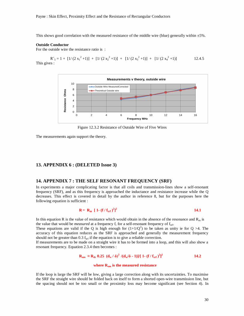
Figure 12.3.2 Resistance of Outside Wire of Five Wires
The measurements again support the theory.
13. APPENDIX 6 : (DELETED Issue 3)
14. APPENDIX 7 : THE SELF RESONANT FREQUENCY (SRF)
In experiments a major complicating factor is that all coils and transmission-lines show a self-resonant
frequency (SRF), and as this frequency is approached the inductance and resistance increase while the Q
decreases. This effect is covered in detail by the author in reference 8, but for the purposes here the
following equation is sufficient :
R = Rm [ 1- (f / fsrf )2]2 14.1
In this equation R is the value of resistance which would obtain in the absence of the resonance and Rm is
the value that would be measured at a frequency f, for a self-resonant frequency of fsrf.
These equations are valid if the Q is high enough for (1+1/Q2) to be taken as unity ie for Q >4. The
accuracy of this equation reduces as the SRF is approached and generally the measurement frequency
should not be greater than 0.3 fsrf if the equation is to give a reliable correction.
If measurements are to be made on a straight wire it has to be formed into a loop, and this will also show a
resonant frequency. Equation 2.3.4 then becomes :
Rom ≈ Rdc 0.25 (dw / δ)2 /(dw/δ - 1)]/[ 1- (f / fsrf )
2]
2 14.2
where Rom is the measured resistance
If the loop is large the SRF will be low, giving a large correction along with its uncertainties. To maximise
the SRF the straight wire should be folded back on itself to form a shorted open-wire transmission line, but
the spacing should not be too small or the proximity loss may become significant (see Section 4). In
Payne : Skin Effect, Proximity Effect and the Resistance of Rectangular Conductors
31
applying the above equations previous experience with transmission lines (as against coils) showed that
best accuracy was achieved if the SRF was assumed to be 85% of the measured value.
Although the SRF can be calculated, it is often best measured because even a very small stray capacitance
in the test jig can significantly reduce its value. Clearly the measurement must be done in exactly the same
jig as that used for the resistance mesurements.
15. APPENDIX 8 : SERIES LIMIT
Equation 5.2.3 gives the resistance of n wires as :
R /Ro = 1 + 2 [1/ (2 n12 +1)] + [1/ (2 n2
2 +1)] + [1/ (2 n3
2 +1)] + [1/ (2 n4
2 +1)] ………15.1
Where n1, n2 .. are integers.
This is a convergent series and it is useful to determine the limit for an infinite number of wires. Ref 11
gives the following equality :
∞
∑ y/(n2+y
2) = -1/(2y) + (π/2) coth (πy) 15.2
n=1
Now 1/(2 n2 +1) = (1/2)/{ n
2 +(1/2)}, so y = 1/√2 in Equation 15.2. Thus :
∞
∑ [1/(2 n2 +1)] = 1/(√2)[-√2/2 + (π/2) coth (πy) = 0.637 15.3
n=1
So Equation 15.1 becomes in the limit i.e. a strip with an infinite number of wires (n=∞) :
R /Ron = 1 + 2 (0.637) = 1.274 15.4
Where Ron is the parallel resistance of n wires, assuming the current is the
same in each.
Payne : Skin Effect, Proximity Effect and the Resistance of Rectangular Conductors
32
REFERENCES
1. WHEELER H A : ‘Formulas for the Skin Effect’, Proc. IRE, September 1942 p412-424.
2. RAMO S & WHINNERY J R : ‘Fields and Waves in Modern Radio’ Second Edition, 1962, John
Wiley & Sons.
3. TERMAN F E : ‘Radio Engineer’s Handbook’, First Edition 1943, McGraw-Hill Book Company.
4. BUTTERWORTH S : ‘Eddy-Current Losses in Cylindrical Conductors, with Special Application
to the Alternating Current Resistance of Short Coils’, Proceedings of the Royal Society, June
1921. http://rsta.royalsocietypublishing.org/content/222/594-604/57.full.pdf+html
5. BUTTERWORTH S : ‘On the Alternating Current Resistance of Solenoid Coils’, Proceedings of
the Royal Society, Vol 107, P693-715. 1925.
6. MOULLIN E B :’Radio Frequency Measurements’, Second Edition, 1931, Charles Griffin &
Company Ltd.
7. WOODRUFF L F : ‘Principles of Electric Power Transmission’, Second Edition, 1938, John
Wiley & Sons Inc.
8. PAYNE A N : ‘Self-Resonance in Single Layer Coils’, http://g3rbj.co.uk/
9. HARNWELL G P : ‘Principles of Electricity and Electromagnetism’, Second Edition, 1949,
McGraw-Hill Book Co Inc.
10. SPREEN J H : ‘A Circuit Approach to Teaching Skin Effect’
http://ilin.asee.org/Conference2007program/Papers/Conference%20Papers/Session%201A/Spreen.
11. http://en.wikipedia.org/wiki/List_of_mathematical_series#cite_note-5
12. PAYNE A N : ‘Skin Effect : Electromagnetic wave or Diffusion ?’ http://g3rbj.co.uk/
13. PAYNE A N : ‘The ac Resistance of Rectangular Conductors’ http://g3rbj.co.uk/
14. SCHRODER G, KAUMANNS J : ‘ Advanced Measurement of ac Resistance on Skin-effect
Reduced Large Conductor Power Cables’ : 8th International Conference on Insulated Power
Cables, A.8.2, June 2011.
http://www.suedkabel.de/cms/upload/pdf/jicable/advanced_measurement_of_AC_resistance_on_s
kin-effect_reduced_large_conductor_power_cables.pdf
Issue 1 : December 2014
Issue 2 : March 2015 : Series Limit determined accurately in Appendix 8, and incorporated into
Equations 5.4.1, 6.2.3, 6.3.3, 7.1.4, 7.1.5, and 7.1.6.
Issue 3 : June 2016 : Resistance of a strip conductor totally revised (Section 6).
© Alan Payne 2016
Alan Payne asserts the right to be recognized as the author of this work.
Enquiries to [email protected]