Skating to Where the

Puck is Going

Aggregate Supply and

Aggregate Demand

Chapter 4

LEARNING OBJECTIVES

Aggregate Supply and supply shocks

Aggregate Demand and a list demand shock

Use matches and mismatches between

aggregate supply and aggregate demand

to explain the “Yes” and “No” answers to

the fundamental macroeconomic question

“Yes” and “No” answers about origins,

expectations, and market responses to

business cycles

continued…

IF YOU PLAN AND BUILD IT . . . AGGREGATE SUPPLY

Supply plans for existing inputs determine aggregate quantity supplied.

Supply plans to increase quantity and quality of inputs,

together with supply shocks, change aggregate supply.

Fig. 4.1: Enlarged GDP Circular Flow of Income and Spending ($)

AGGREGATE SUPPLY (AS)

Macroeconomic players

consumers, businesses, government make

two kinds of plans for supplying Canadian

real GDP

a) supply plans for existing inputs

b) supply plans to increase inputs

a) Supply plans for existing inputs similar to microeconomic choices about quantity supplied

Aggregate quantity suppliedquantity of real GDP players plan to supply at different average price levels

Law of aggregate supplyas average level of prices rises, aggregate quantity supplied increases (up to maximum of potential GDP)

b) Supply plans to increase quantity or quality

of inputs cause increase in aggregate

supply — increase in economy’s capacity to

produce real GDP

With existing inputs Increasing input (quality & quantity)

Business supply choices

what to produce, quantities to produce, quantities of inputs to

hire.

new factories/equipment,

resources, technology.

Consumer supply choices

participate in labour force, hours to work,

inputs to supply.

having children, education and

training.

Government supply choices

resources to supply.Determines aggregate

quantity supplied

infrastructure, rules of the game, policies

Outcome Determines aggregate quantity supplied.

Changes AS and increases potential GDP.

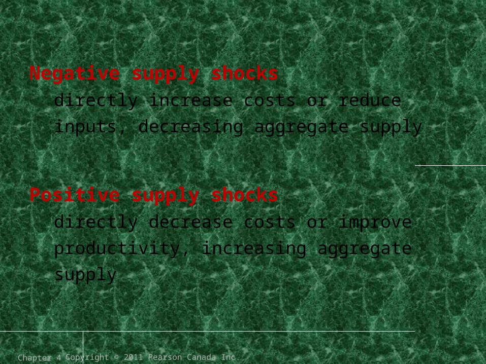
Negative supply shocks directly increase costs or reduce inputs,

decreasing aggregate supply

Positive supply shocks directly decrease costs or improve

productivity, increasing aggregate supply

The Law of Aggregate Supply

The aggregate quantity supplied of Real GDP

Decreases if:• average level of prices falls

Increases if:• average level of prices rises

Changes in Aggregate Supply

The aggregate supply of Real GDP

Decreases if:• negative supply shock raises

price for resource inputs• negative supply shock

destroys inputs

Increases if:• businesses plan to increase

quantity or quality inputs• positive supply shock lowers

price for resource inputs• positive supply shock

improves technologies

Fig. 4.2: Law of Aggregate Supply and Changes in AS

. . . WILL THEY COME AND BUY IT? AGGREGATE DEMAND

Demand plans determine aggregate quantity demanded.

Demand shocks — from changes in expectations, interest rates, government policy, GDP in R.O.W.,

exchange rates — change aggregate demand.

AGGREGATE DEMAND (AD)

All macroeconomic players —

consumers, businesses, government, R.O.W.

make demand plans for spending, like

microeconomic choices about quantity

demanded

Aggregate quantity demandedquantity of real GDP players plan to demand at different average price levels

Law of aggregate demandas average level of prices rises, aggregate quantity demanded decreases

a. Consumers plans to spend (C) a fraction of

disposable income

b.Businesses plan investment spending (I)

for new factories and equipment. I plans are

volatile.

c. Government spending plans (G) for

products/services set by budget

d.R.O.W. spending plans (X) for Canadian exports

subtract imports (IM) from all other planned spending to get net exports (X — IM) = difference between what Canada exports and imports

Planned spending on aggregate demand =

planned C + planned I + planned G +

planned (X − IM)

Demand shocks

factors, other than average prices, changing

aggregate demand

Aggregate demand changes with expectations,

interest rates, government policy, GDP in

R.O.W., exchange rates

Negative demand shocks decrease

aggregate demand

a) more pessimistic expectations

b) higher interest rates

c) lower government spending and/or higher

taxes

d) decreased GDP in R.O.W.

e) higher value Canadian dollar

Positive demand shocks increase aggregate

demand

f) more optimistic expectations

g) lower interest rates

h) higher government spending and/or lower

taxes

i) increased GDP in R.O.W.

j) lower value Canadian dollar

MATCH OR MISMATCH? AGGREGATE SUPPLY & AGGREGATE

DEMAND

Matches between aggregate supply and aggregate demand

give equilibrium, Say’s Law, and “Yes” answer; mismatches give Keynes’s business cycles,

demand and supply shocks, and “No” answer.

“Yes” “No”

AGGREGATE SUPPLY & AGGREGATE DEMAND

“Yes” answermacroeconomic equilibrium with existing inputs when aggregate demand matches aggregate supply

– AS choices based on expectations of what price level and aggregate demand will be when products/services get to market

– price level and AD what suppliers expected

– Real GDP = potential GDP; inputs fully employed

– Say’s Law — supply creates its own demand

continued…

“Yes” answer

equilibrium over time with increasing inputs

when aggregate demand matches aggregate

supply

– add savings and investment to explain growth in living standards over time (real GDP per person)

– savings threaten Say’s Law, since all income in input markets not spent demanding products/services in output markets

continued…

Market for loanable fundsbanks coordinate supply of loanable funds

(savings) with demand for loanable funds

(borrowing)

– interest rate is price of loanable funds

– if banks loan savings to businesses that use it for investment spending, offsets consumer savings, restoring equality between aggregate income and aggregate spending

Investment spending increases inputs, so

potential GDP and real GDP per person increase

over time

– aggregate supply and aggregate demand both increase, full employment continues, average prices stay stable

“No” answer

mismatch between aggregate demand and

aggregate supply

– aggregate supply choices based on expectations of what price level and aggregate demand will be when products/services get to market

– expectations disappointed,outcomes do not work out as planned

– adjustments — expansions and contractions — necessary to get back to smart choices

– Keynes’s business cycles

Mismatch scenarios from demand shocks

– negative demand shock causes recessionary gap — falling average prices, decreased real GDP, increased unemployment

– positive demand shock causes inflationary gap —rising average prices increased real GDP, decreased unemployment

– demand shocks cause unemployment and inflation to move in opposite directions, like Philips Curve

Mismatch scenarios from supply shocks

– negative supply shock causes stagflation —rising average prices, decreased real GDP, increased unemployment

– positive supply shock causes falling average prices, increased real GDP, decreased unemployment

– supply shocks cause unemployment and inflation to move in same direction

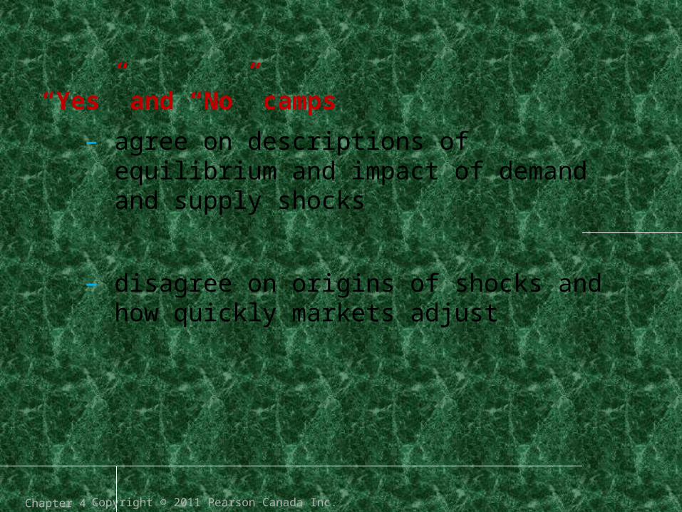
“Yes” and “No” camps

– agree on descriptions of equilibrium and impact of demand and supply shocks

– disagree on origins of shocks and how quickly markets adjust

SHOCKING STARTS AND FINISHES: ORIGINS AND RESPONSES TO BUSINESS

CYCLES

“Yes” and “No” camps disagree about external/internal

origins of shocks, about rational/volatile expectations, and about how quickly price adjustments

restore match between aggregate supply and demand.

“Yes” camp

markets quickly self-adjust, so hands-off

– origins of shocks external to economy — nature, science, mistaken government policies

– government part of problem, not solution

– rational expectations and logical choices

ORIGINS AND RESPONSES TO BUSINESS CYCLES

• For “Yes” camp, when shocks occur, price

adjustments in all markets quickly restore

match between aggregate supply and

aggregate demand — example of negative

demand shock

– in labour market, unemployment causes wages to fall, increasing hiring back to full employment

– in output markets, prices fall due to surpluses and falling wage costs, increasing sales back to potential GDP

– in international trade market,

falling Canadian prices increase net exports,

increasing Canadian real GDP and decreasing

unemployment

– in loanable funds market, savings cause

interest rates to fall, increasing investment

spending (I), increasing Canadian real GDP

and

decreasing unemployment

“No” camp

markets fail to quickly self-adjust, so hands-on

– origins of shocks internal to economy — changing expectations, role of money, connections with R.O.W.

– volatile expectations based on fundamental uncertainty about future

– facing uncertainty, saving decisions are internal negative demand shock

– business cycles in other economies affect Canada through exports and imports

For “No” camp, when shocks occur, difficult

adjustments in all markets — example of

negative demand shock

– in labour market, wages sticky even with unemployment —layoffs instead of lower wages

– in output markets, prices fall due to surpluses,

but falling incomes from unemployment in input markets decrease consumption demand (C)

– in international trade market, falling Canadian prices increase net exports, but destabilizing effects of cycles in R.O.W.

– in loanable funds market, even if interest rates fall, pessimistic expectations may cause investment spending (I) to decrease

– with weak/slow price adjustments, role for government to bring aggregate supply and aggregate demand back into balance

Disagreement between “Yes” and “No”

camps on

– connections between input markets and output markets for both demand and supply sides

– connections between Canada and R.O.W.

– connections between money/banks/expectations and input and output markets

Fig. 4.8 Origins of Shocks and Business Cycles