Embed Size (px)
Citation preview
Sizing of a 3,000,000t Bulk Cargo Port through Discrete and Stochastic
Simulation Integrated with Response Surface Methodology Techniques
L. CASSETTARI, R. MOSCA, R. REVETRIA
DIPTEM – Department of Production Engineering, Thermoenergetics and Mathematical Models
University of Genoa
Via all’Opera Pia 15, 16145 Genova (GE)
ITALY
[email protected], [email protected], [email protected]
F. ROLANDO
Duferco Engineering S.p.A.
Via Paolo Imperiale 4/14, 16126 Genova (GE)
ITALY
Abstract: - The purpose of the study is to size, by means of a discrete and stochastic simulator, a bulk cargo
port for the unloading of coal to cover the annual requirements of a thermal power plant located next to the
berth. The logistics system under consideration had to be designed so that it could ensure the supply of enough
coal for the operation of the plant while reducing the overall operating costs of the system (freightage,
demurrage for delays in unloading operations, investment costs, overheads) to a minimum. Thanks to Design of
Experiments (DOE) and Response Surface Methodology (RSM), it was possible to determine the mathematical
relationship, in the form of regression meta-model, existing between the design variables and the target
function consisting in the overall annual operating cost. After the sizing it has been finally done an analysis of
the strength of the identified solution as the needs for coal on the part of the power plant, with a specific
reference to the capacity of the intermediate accumulation tank which constitutes a critical element in the
design of this type of plants.
Key-Words: Bulk Cargo Port Design, Discrete and Stochastic Simulation, Mean Square Pure Error Evolution,
Response Surface Methodology
1 Introduction The installation of a new thermal power plant close
to the sea makes it necessary the sizing of a bulk
cargo port for the unloading of the coal to feed the
steam production plant.
Fig. 1
On the basis of a financial plan which takes into
consideration, on one side the demurrage costs and
on the other side the costs linked to the investment
and to the management of the site, we have arrived
to the optimal design of the following elements: - Number of docks;
- Mix of incoming ships;
- Number and capacity of berth grab cranes;
- Capacity and number of domes used.
The presence of stochastic variables linked to the
ships’ interarrival laws, to the breakdowns and to
the maintenance of the different installations present
in the unloading and transportation system have
made it necessary to undertake the study with the
construction of a discrete and stochastic simulation
model. The software used to build the model is
Flexsim 5.0.4 by Flexsim Software Products, Inc.
2 Model description
In the plant under study, coal is shipped by means of
bulk carriers of different tonnage and from different
Recent Advances in Signal Processing, Computational Geometry and Systems Theory
ISBN: 978-1-61804-027-5 211
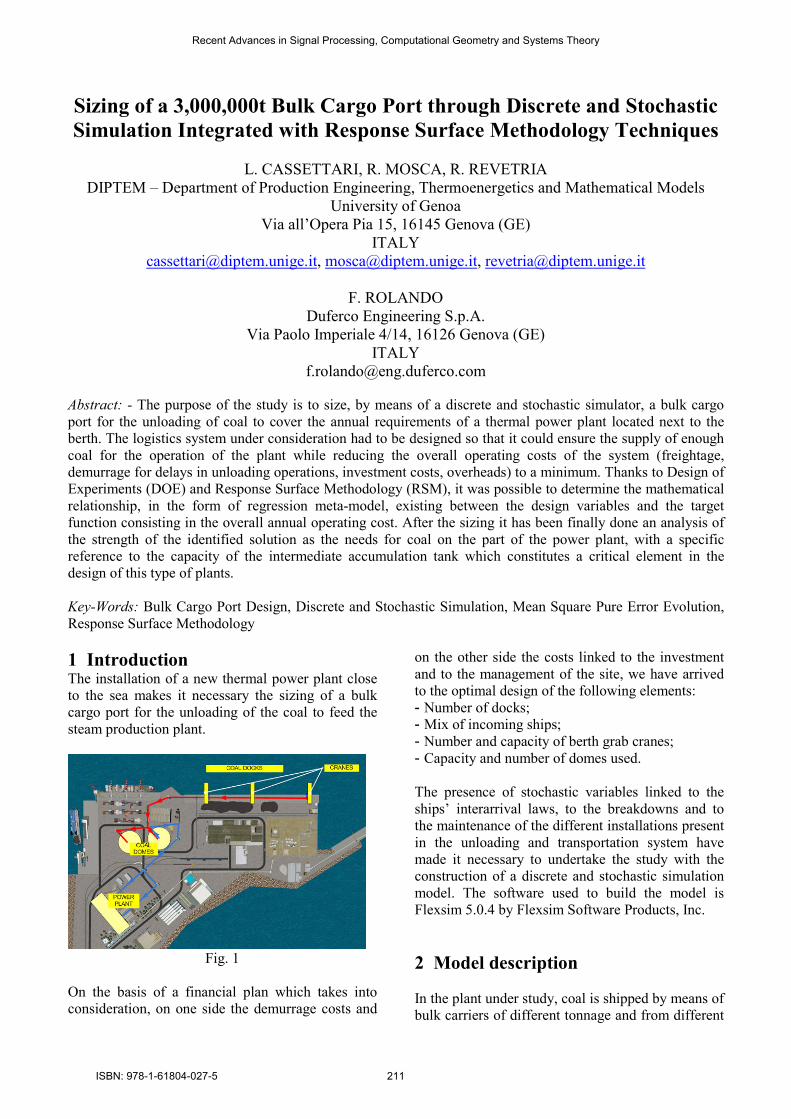
places in the world; it is unloaded by means of port
unloading equipment (grab cranes) that feeds a
system of conveyor belts, which carry the coal to an
intermediate storage system (domes) and/or feed it
to the furnace bunkers serving the plant. Figure 1
shows the plan of the complex as described in the
simulation model.
2.1 The ships In the model we have used the following standard
types of ocean-going vessels:
- Barge;
- Handysize;
- Panamax;
- Capesize;
The table 1 shows the main features of the type of
vessels listed here above:
Table 1
The ships’ mix, that is the share of coal transported
by the various types of ship, influences the
performances of the system in terms of:
- freight costs, which are in inverse relation to the
transported quantity of coal (DWT);
- demurrage days, which are in direct relation to the
tonnage;
- dredging works and the sea bottom, which restrain
the types of ship that can dock;
- number and unloading logics of the harbour
cranes.
The cargo in each hold is made up by a number of
discrete units (flowitems) obtained by the ratio
between the tonnage contents of the hold and the
capacity of the bucket of the grab crane (a parameter
that can be set by GUI). This solution has been
adopted in order to be able to replicate the correct
unloading of the ships; this way in fact the grab
cranes execute a number of cycles equal to the
number of “bucket-loads” necessary to unload a
ship.
The unloaded flowitems are later converted into
fluid units by a specific object (itemtofluid), which,
for each unloaded discrete unit, generates a number
of fluid units equal to the capacity of the bucket.
The number of ships has been calculated on the
basis of the yearly coal needs of the power station,
of the DWT and of the mix utilized. Given:
- Ci (1 ≤ i ≤ 4): the capacity of the ships for each
type;
- Ctot: the yearly coal needs;
- a, b, c, d: the percentages to be utilized for each
type of ships;
the yearly number of ships, for each type (Ni)
results from solving the following linear system: C1 C2 C3 C4 0 N1 Ctot
1 0 0 0 -a N2 0
0 1 0 0 -b N3 0
0 0 1 0 -c N4 0
0 0 0 1 -d NTOT 0
(1)
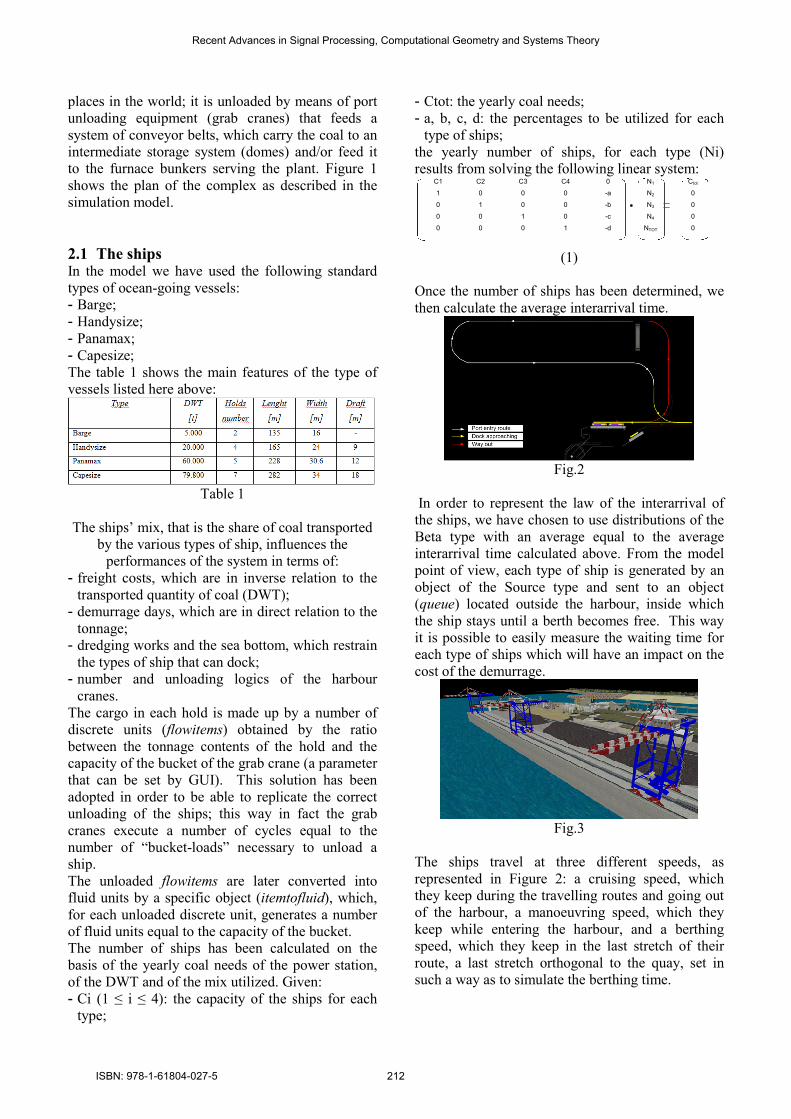
Once the number of ships has been determined, we
then calculate the average interarrival time.
Fig.2
In order to represent the law of the interarrival of
the ships, we have chosen to use distributions of the
Beta type with an average equal to the average
interarrival time calculated above. From the model
point of view, each type of ship is generated by an
object of the Source type and sent to an object
(queue) located outside the harbour, inside which
the ship stays until a berth becomes free. This way
it is possible to easily measure the waiting time for
each type of ships which will have an impact on the
cost of the demurrage.
Fig.3
The ships travel at three different speeds, as
represented in Figure 2: a cruising speed, which
they keep during the travelling routes and going out
of the harbour, a manoeuvring speed, which they
keep while entering the harbour, and a berthing
speed, which they keep in the last stretch of their
route, a last stretch orthogonal to the quay, set in
such a way as to simulate the berthing time.
Recent Advances in Signal Processing, Computational Geometry and Systems Theory
ISBN: 978-1-61804-027-5 212
2.2 The grab cranes The unloading infrastructure envisages a maximum
of no.3 grab cranes of the type with a fixed winch
and raisable arm, as shown in Figure 3, with an
unloading rate which can be set as a working
parameter of the model.
The effective unloading rate is a function of the
“free-digging” rate, that is the theoretical unloading
rate that can be obtained under maximum efficiency
conditions, according to the following reduction
coefficients:
- Opening time of the hold hatches: 0.85
- Weather conditions: 0.95
- Emergency maintenance (breakdowns): 0.95
- Holds cleaning: 0,85
- Yield in filling the bucket: 0.92.
Therefore the effective rate comes to about 60% of
the “free-digging” rate.
In order to implement this logic into the model it has
been necessary to carry out a series of experiments
to measure the cycle time for different settings of
some parameters. In consideration of the importance
of the grab cranes, we have chosen to create ad hoc
objects that could reproduce faithfully the
movements of the cranes and the respective action
times.
Such objects offer the possibility of obtaining
different cycle times acting mainly on only two
factors: the bucket capacity, that is the tons/cycle
unloaded at each trip, and the four typical speeds
(the crane transverse motion speed, the trolley
speed, the lifting speed and the descent speed). To
set the different simulation scenarios we have
chosen, once the bucket capacity has been set, to
keep unchanged the crane translation and trolley
speeds and to derive a relationship linking the
downloading rate and the lifting speed.
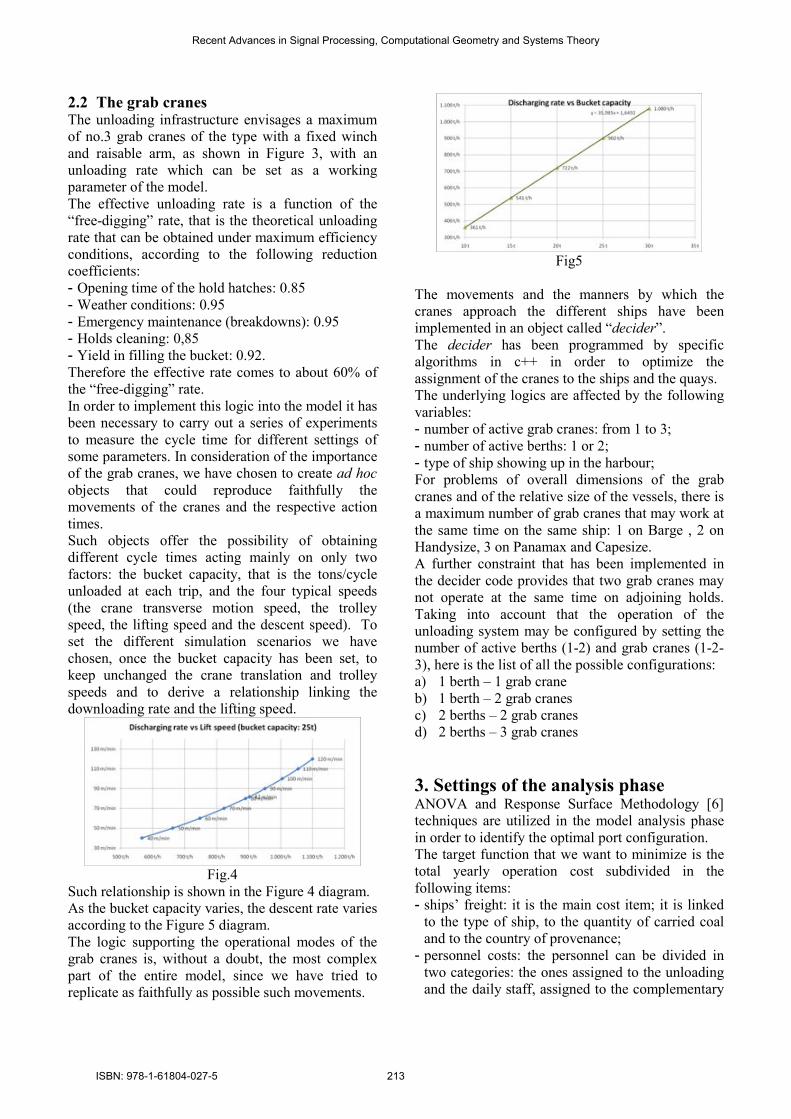
Fig.4
Such relationship is shown in the Figure 4 diagram.
As the bucket capacity varies, the descent rate varies
according to the Figure 5 diagram.
The logic supporting the operational modes of the
grab cranes is, without a doubt, the most complex
part of the entire model, since we have tried to
replicate as faithfully as possible such movements.
Fig5
The movements and the manners by which the
cranes approach the different ships have been
implemented in an object called “decider”.
The decider has been programmed by specific
algorithms in c++ in order to optimize the
assignment of the cranes to the ships and the quays.
The underlying logics are affected by the following
variables:
- number of active grab cranes: from 1 to 3;
- number of active berths: 1 or 2;
- type of ship showing up in the harbour;
For problems of overall dimensions of the grab
cranes and of the relative size of the vessels, there is
a maximum number of grab cranes that may work at
the same time on the same ship: 1 on Barge , 2 on
Handysize, 3 on Panamax and Capesize.
A further constraint that has been implemented in
the decider code provides that two grab cranes may
not operate at the same time on adjoining holds.
Taking into account that the operation of the
unloading system may be configured by setting the
number of active berths (1-2) and grab cranes (1-2-
3), here is the list of all the possible configurations:
a) 1 berth – 1 grab crane
b) 1 berth – 2 grab cranes
c) 2 berths – 2 grab cranes
d) 2 berths – 3 grab cranes
3. Settings of the analysis phase ANOVA and Response Surface Methodology [6]
techniques are utilized in the model analysis phase
in order to identify the optimal port configuration.
The target function that we want to minimize is the
total yearly operation cost subdivided in the
following items:
- ships’ freight: it is the main cost item; it is linked
to the type of ship, to the quantity of carried coal
and to the country of provenance;
- personnel costs: the personnel can be divided in
two categories: the ones assigned to the unloading
and the daily staff, assigned to the complementary
Recent Advances in Signal Processing, Computational Geometry and Systems Theory
ISBN: 978-1-61804-027-5 213
operations (cleaning the holds, cleaning the
conveying belts, maintenance, control, and so on).
- maintenance costs for the grab cranes, conveying
belts, stacker-reclaimer, electric systems, lighting
systems, firefighting systems;
- depreciation allowances for civil constructions (20
years), grab cranes (10 years), domes (15 years),
conveyor belts, towers and other facilities (10
years);
- demurrage, the cost of which depends on the type
of ship, according to Table 2:
Table 2
- cleaning costs for the holds and the conveyor belts.
As already evidenced in the introduction, the project
variables to dimension as a function of the operation
costs are the number of berths, the number of grab
cranes and their unloading rate, the ships’ mix and
the storage capacity of the domes.
Since the number of berths (1 or 2) also conditions,
as we have already said before, the number of grab
cranes, we have decided to consider this factor as a
scenario variable. The final decision, therefore, will
be taken by comparing the optimum solution of the
first scenario with the optimum solution of the
second one, and of the two we shall choose the one
considered as more favourable.
The storage capacity of the domes has shown itself
to be a determinant factor. often the demurrage
values obtained with the simulator reached very
high figures because of the frequent stops of the
unloading system caused by an insufficient capacity
of intermediate storage. We have therefore decided
to initially set the storage capacity to infinity, and to
determine afterwards the size of the dome on the
base of the actual utilization demand thereof as
explained further on.
Therefore the focus of the testing moves to the grab
cranes and to the ships’ mix for which it has been
necessary to define a range of variability.
As to the grab cranes, however, we have assumed as
a summary variable of their behaviour the unloading
capacity, that is a combination between the
unloading rate and the number of grab cranes. In
particular, in correspondence of the first scenario (a
single berth), the variability ranges are:
- Lower level: 1 grab crane, free-digging rate 1,500
t/h;
- Higher Level: 2 grab cranes, free-digging rate
1,900 t/h each;
While in the second scenario (two berths) they are:
- Lower level: 2 grab cranes, free-digging rate:
1,500 t/h each;
- Higher Level: 3 grab cranes, free-digging rate:
1,900 t/h each;
In both scenarios the grab cranes work for 2 shifts
per day of 8 hrs each, for 5 days a week, Monday to
Friday.
For the variable “ships’ mix” we have assumed to
consider as lower level the configuration in which
there arrive mostly small ships (of the Handysize
type) and as higher level the one in which there
arrive bigger ships on average (Table 3).
Unlike what we have said for the grab cranes, the
range of the variable “ships’ mix” remains the same
in both scenarios. The two ends of the range are
represented by the following percentages:
Table 3
3.1 Scenario with 1 berth
3.1.1 Determination of the length of the
simulation run
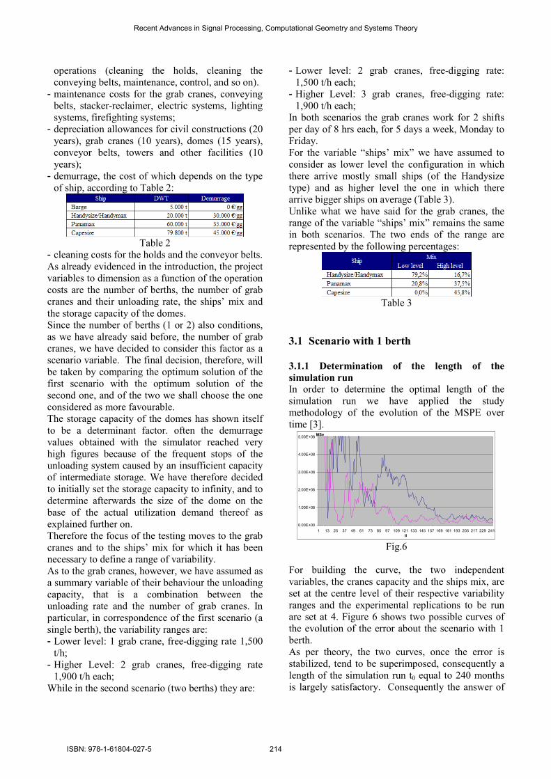
In order to determine the optimal length of the
simulation run we have applied the study
methodology of the evolution of the MSPE over
time [3].
0.00E+00
1.00E+08
2.00E+08
3.00E+08
4.00E+08
5.00E+08
1 13 25 37 49 61 73 85 97 109 121 133 145 157 169 181 193 205 217 229 241
ti
MSe
Fig.6
For building the curve, the two independent
variables, the cranes capacity and the ships mix, are
set at the centre level of their respective variability
ranges and the experimental replications to be run
are set at 4. Figure 6 shows two possible curves of
the evolution of the error about the scenario with 1
berth.
As per theory, the two curves, once the error is
stabilized, tend to be superimposed, consequently a
length of the simulation run t0 equal to 240 months
is largely satisfactory. Consequently the answer of
Recent Advances in Signal Processing, Computational Geometry and Systems Theory
ISBN: 978-1-61804-027-5 214
the simulator will show an error band of the type of
(2):
)(3)()(*)(3)( 0000 tMSPEtytytMSPEty o +≤≤−
(2)
In the case under examination, since the MSPE
(240) is about 1.4·107 the bandwidth is equal to ±
11.000 €, a value that has a negligible impact on an
average monthly demurrage cost of about 273,000€.
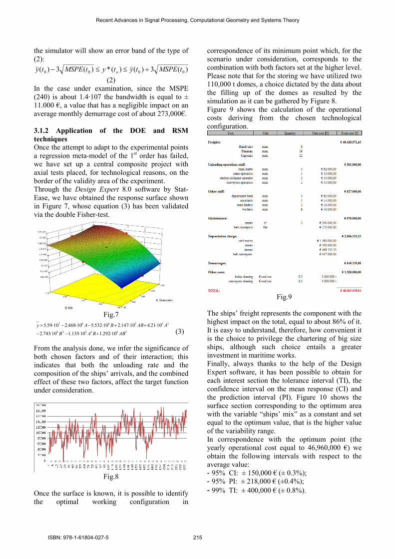
3.1.2 Application of the DOE and RSM
techniques
Once the attempt to adapt to the experimental points
a regression meta-model of the 1st order has failed,
we have set up a central composite project with
axial tests placed, for technological reasons, on the
border of the validity area of the experiment.
Through the Design Expert 8.0 software by Stat-
Ease, we have obtained the response surface shown
in Figure 7, whose equation (3) has been validated
via the double Fisher-test.
Fig.7
(3)
From the analysis done, we infer the significance of
both chosen factors and of their interaction; this
indicates that both the unloading rate and the
composition of the ships’ arrivals, and the combined
effect of these two factors, affect the target function
under consideration.
Fig.8
Once the surface is known, it is possible to identify
the optimal working configuration in
correspondence of its minimum point which, for the
scenario under consideration, corresponds to the
combination with both factors set at the higher level.
Please note that for the storing we have utilized two
110,000 t domes, a choice dictated by the data about
the filling up of the domes as resulted by the
simulation as it can be gathered by Figure 8.
Figure 9 shows the calculation of the operational
costs deriving from the chosen technological
configuration.
Fig.9
The ships’ freight represents the component with the
highest impact on the total, equal to about 86% of it.
It is easy to understand, therefore, how convenient it
is the choice to privilege the chartering of big size
ships, although such choice entails a greater
investment in maritime works.
Finally, always thanks to the help of the Design
Expert software, it has been possible to obtain for
each interest section the tolerance interval (TI), the
confidence interval on the mean response (CI) and
the prediction interval (PI). Figure 10 shows the
surface section corresponding to the optimum area
with the variable “ships’ mix” as a constant and set
equal to the optimum value, that is the higher value
of the variability range.
In correspondence with the optimum point (the
yearly operational cost equal to 46,960,000 €) we
obtain the following intervals with respect to the
average value:
- 95% CI: ± 150,000 € (± 0.3%);
- 95% PI: ± 218,000 € (±0.4%);
- 99% TI: ± 400,000 € (± 0.8%).
262526
255667
10292.110135.110743.2
1021.410147.210532.510468.21059.5
ABBAB
AABBAy
⋅+⋅−⋅−
⋅+⋅+⋅−⋅−⋅=
Recent Advances in Signal Processing, Computational Geometry and Systems Theory
ISBN: 978-1-61804-027-5 215
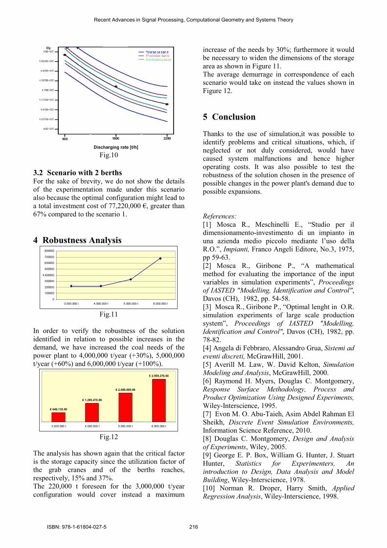
Fig.10
3.2 Scenario with 2 berths For the sake of brevity, we do not show the details
of the experimentation made under this scenario
also because the optimal configuration might lead to
a total investment cost of 77,220,000 €, greater than
67% compared to the scenario 1.
4 Robustness Analysis
0
100000
200000
300000
400000
500000
600000
700000
800000
3.000.000 t 4.000.000 t 5.000.000 t 6.000.000 t
t
Fig.11
In order to verify the robustness of the solution
identified in relation to possible increases in the
demand, we have increased the coal needs of the
power plant to 4,000,000 t/year (+30%), 5,000,000
t/year (+60%) and 6,000,000 t/year (+100%).
€ 649,135.00
€ 1,295,470.00
€ 2,006,695.00
€ 2,959,276.00
3.000.000 t 4.000.000 t 5.000.000 t 6.000.000 t
Fig.12
The analysis has shown again that the critical factor
is the storage capacity since the utilization factor of
the grab cranes and of the berths reaches,
respectively, 15% and 37%.
The 220,000 t foreseen for the 3,000,000 t/year
configuration would cover instead a maximum
increase of the needs by 30%; furthermore it would
be necessary to widen the dimensions of the storage
area as shown in Figure 11.
The average demurrage in correspondence of each
scenario would take on instead the values shown in
Figure 12.
5 Conclusion
Thanks to the use of simulation,it was possible to
identify problems and critical situations, which, if
neglected or not duly considered, would have
caused system malfunctions and hence higher
operating costs. It was also possible to test the
robustness of the solution chosen in the presence of
possible changes in the power plant's demand due to
possible expansions.
References:
[1] Mosca R., Meschinelli E., “Studio per il
dimensionamento-investimento di un impianto in
una azienda medio piccolo mediante l’uso della
R.O.”, Impianti, Franco Angeli Editore, No.3, 1975,
pp 59-63.
[2] Mosca R., Giribone P., “A mathematical
method for evaluating the importance of the input
variables in simulation experiments”, Proceedings
of IASTED "Modelling, Identification and Control",
Davos (CH), 1982, pp. 54-58.
[3] Mosca R., Giribone P., “Optimal lenght in O.R.
simulation experiments of large scale production
system”, Proceedings of IASTED "Modelling,
Identification and Control", Davos (CH), 1982, pp.
78-82.
[4] Angela di Febbraro, Alessandro Grua, Sistemi ad
eventi discreti, McGrawHill, 2001.
[5] Averill M. Law, W. David Kelton, Simulation
Modeling and Analysis, McGrawHill, 2000.
[6] Raymond H. Myers, Douglas C. Montgomery,
Response Surface Methodology, Process and
Product Optimization Using Designed Experiments,
Wiley-Interscience, 1995.
[7] Evon M. O. Abu-Taieh, Asim Abdel Rahman El
Sheikh, Discrete Event Simulation Environments,
Information Science Reference, 2010.
[8] Douglas C. Montgomery, Design and Analysis
of Experiments, Wiley, 2005.
[9] George E. P. Box, William G. Hunter, J. Stuart
Hunter, Statistics for Experimenters, An
introduction to Design, Data Analysis and Model
Building, Wiley-Interscience, 1978.
[10] Norman R. Droper, Harry Smith, Applied
Regression Analysis, Wiley-Interscience, 1998.
Recent Advances in Signal Processing, Computational Geometry and Systems Theory
ISBN: 978-1-61804-027-5 216