Size Biased Lomax Distribution - .:.GC University Lahore 4.pdf · Size Biased Lomax Distribution Muhammad Abdullah1, Zafar Iqbal2, ... [email protected] 2 National College of Business

ISSN 1684-8403

Journal of Statistics

Volume 23, 2016. pp. 32-49

________________________________________________________________________

Size Biased Lomax Distribution

Muhammad Abdullah

1, Zafar Iqbal

2, Azeem Ali

3,

Muhammad Zakria4

and Munir Ahmad5

Abstract

Weighted Distributions have very significant place in the mathematical statistics,

particularly in the case of Unequal Probability Sampling. Size Biased Distribution

is a particular case of Weighted Probability Distribution. In this paper, Size

Biased form of Lomax Probability Distribution is introduced. Some basic

properties of Size Biased Lomax (SBL) are derived. Reliability measures

including the Survival Analysis, Hazard Rate and Vitality functions are computed.

Measures of entropy using Shannon’s and Renyi’s methods are also found.

Estimation of its parameters is made through method of Maximum Likelihood

and Method of Moments. Lomax Distribution has applications in various fields

including size of cities. In this paper, it is showed that SBL fits the data on size of

cities of Pakistan in km2.

Keywords

Lomax Distribution, Survival function, Hazard rate function, Entropy

1. Introduction

Initially, Lomax Distribution was introduced by Lomax (1954) to model the

business failure rate. It is also known as Pareto Type-II Distribution.

_________________________________ 1 Allama Iqbal Open University, Islamabad, Pakistan

Email: [email protected], [email protected] 2

National College of Business Administration and Economics, Lahore, Pakistan

Email: [email protected] 3 Government College University, Lahore, Pakistan

4Allama Iqbal Open University, Islamabad, Pakistan

Email: [email protected], [email protected] 5 National College of Business Administration and Economics, Lahore, Pakistan

Email: [email protected]

mailto:[email protected]




_______________________________________________________________________________ 33

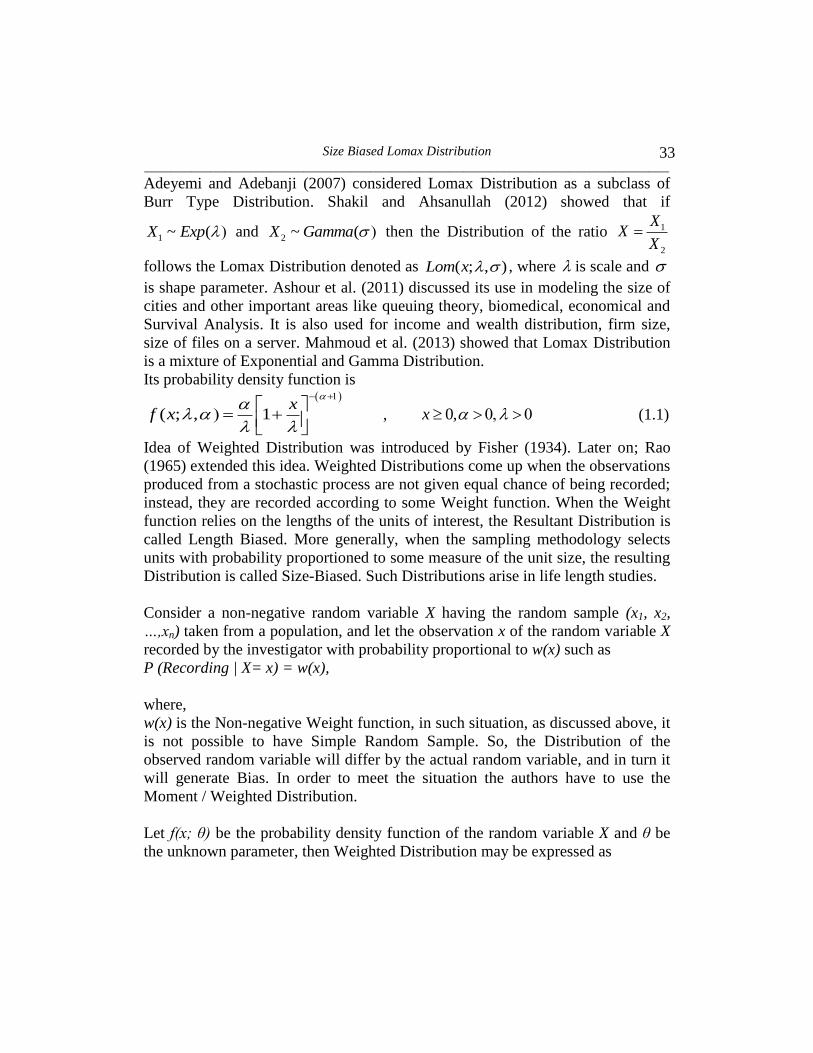
Adeyemi and Adebanji (2007) considered Lomax Distribution as a subclass of

Burr Type Distribution. Shakil and Ahsanullah (2012) showed that if

1 ~ (X Exp and 2 ~ (X Gamma then the Distribution of the ratio 1

2

XX

X

follows the Lomax Distribution denoted as ( ; , )Lom x , where is scale and

is shape parameter. Ashour et al. (2011) discussed its use in modeling the size of

cities and other important areas like queuing theory, biomedical, economical and

Survival Analysis. It is also used for income and wealth distribution, firm size,

size of files on a server. Mahmoud et al. (2013) showed that Lomax Distribution

is a mixture of Exponential and Gamma Distribution.

Its probability density function is

( ; , 1x

f x

, 0,x (1.1)

Idea of Weighted Distribution was introduced by Fisher (1934). Later on; Rao

(1965) extended this idea. Weighted Distributions come up when the observations

produced from a stochastic process are not given equal chance of being recorded;

instead, they are recorded according to some Weight function. When the Weight

function relies on the lengths of the units of interest, the Resultant Distribution is

called Length Biased. More generally, when the sampling methodology selects

units with probability proportioned to some measure of the unit size, the resulting

Distribution is called Size-Biased. Such Distributions arise in life length studies.

Consider a non-negative random variable X having the random sample (x1, x2,

…,xn) taken from a population, and let the observation x of the random variable X

recorded by the investigator with probability proportional to w(x) such as

P (Recording | X= x) = w(x),

where,

w(x) is the Non-negative Weight function, in such situation, as discussed above, it

is not possible to have Simple Random Sample. So, the Distribution of the

observed random variable will differ by the actual random variable, and in turn it

will generate Bias. In order to meet the situation the authors have to use the

Moment / Weighted Distribution.

Let f(x; θ) be the probability density function of the random variable X and θ be

the unknown parameter, then Weighted Distribution may be expressed as

Muhammad Abdullah, Zafar Iqbal, Azeem Ali, Muhammad Zakria and Munir Ahmad

_______________________________________________________________________________

34

( ) ( ; )

( ; )( )

w x f xg x

E w x

(1.2)

Patil and Ord (1976) used w(x) = xm

, and they call it Moment Distribution.

'

( ; )( ; )

m

m

x f xg x

(1.3)

Here, ' ( ; )m

m x f x For discrete case

' ( ; )m

m x f x dx

For continuous case

For m = 1 it’s called the Size/Length Biased

For m = 2 it’s called the area Biased Distribution

Dara (2011) derived various Moment Distributions and their Size-Biased forms

specifically their reliability measures. Nasiri and Hosseini (2012) obtained

Maximum Likelihood Estimates (MLE) and Bayesian Estimates under two loss

functions of parameters of the Lomax Distribution based on record values. Ahmed

et al. (2013) derived a new class of Length-Biased Gamma Distribution and

discussed its structural properties. Hasnain (2013) introduced a new family of

Distributions named as Exponentiated Moment Exponential Distribution (EMED)

and developed its properties. Iqbal, et al. (2013) found a more general class for

EMED and built up different properties including characterization through

conditional moments.

2. Properties of Size Biased Lomax Distribution

The Size Biased form of Lomax Distribution may be obtained as (

2

( 1)( ) 1

xg x x

0, 1, 0x (2.1)

Its cumulative distribution function (c.d.f) is given as

( ) 1 1 1x x

G x

0, 1, 0x (2.2)

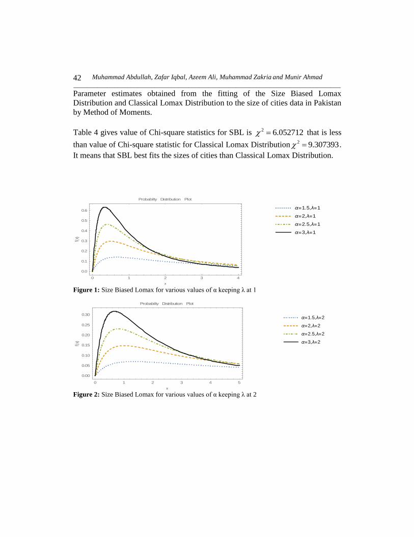
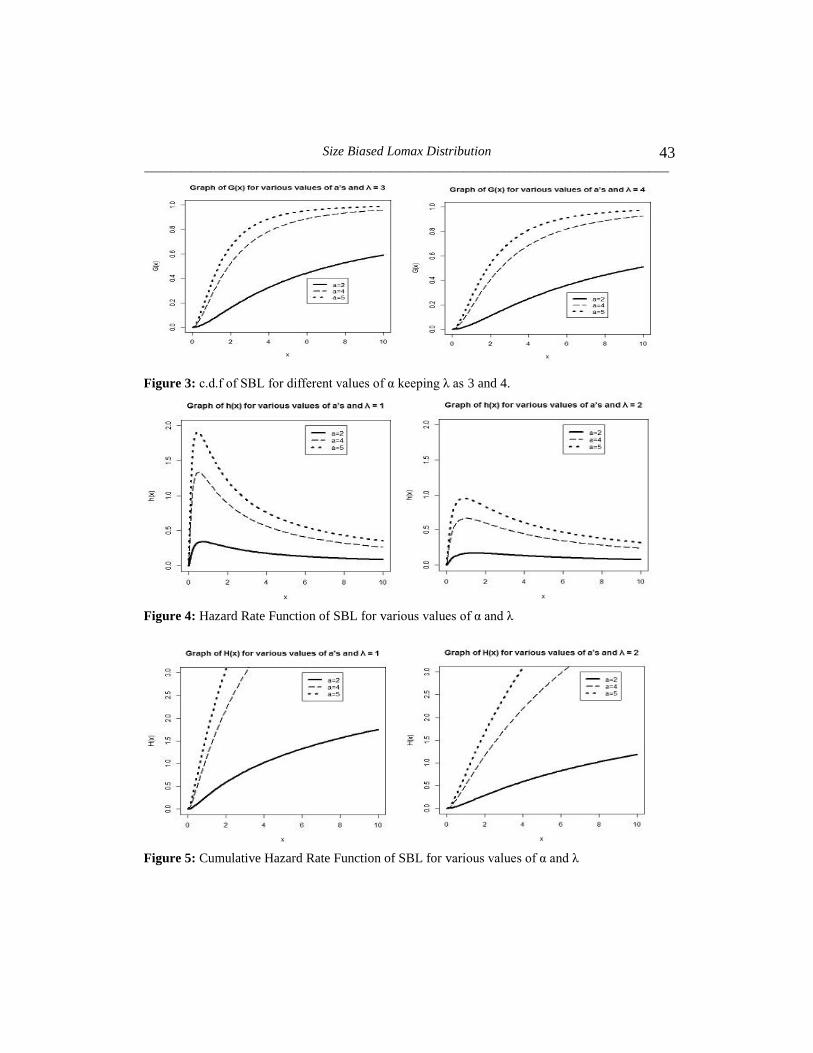
Graph of the p.d.f given by eq. (2.1) is in Figure 1 and 2.


_______________________________________________________________________________ 35

As value of α increase, peak of the graph becomes sharper, and with increase in

value of λ its tail becomes heavy. Graph for Distribution function I given in

Figure 3.

2.1 Hazard Rate Function: Hazard Rate Function also known as failure rate may

be defined as the conditional probability of failure of an item in the interval

[ , ]x x h where 0h given that certain item is existing till age x. it is given as

( ))

( )

f xh x

F x (2.1.1)

It has various names in different areas of study e.g. in actuaries and demography it

is called force to mortality and in extreme value theory it is known as Intensity

Function. It is useful in various fields of life such as Survival Analysis,

biomedical sciences, engineering and in modeling life time data.

Hazard Rate Function for SBL can take the form, 1 1

( 1)( ) 1 1

x x xh x

0, 1, 0x (2.1.2)

Graph of Hazard Rate Function is given in Figure 4.

Hazard Rate Function of SBL Distribution is upside down (bathtub) shaped.

2.2 Cumulative Hazard Function: Cumulative Hazard Function is given as

1

( ) ln

1

x

H xx

0, 1, 0x (2.2.1)

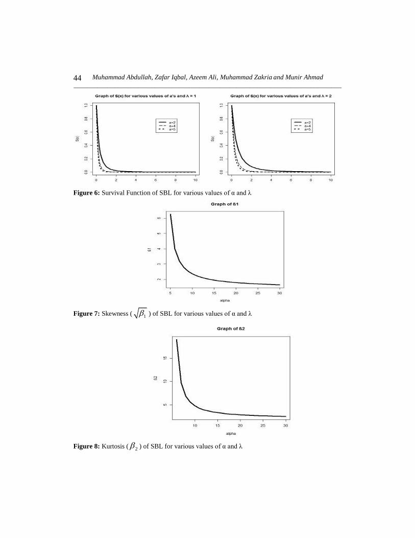
2.3 Survival Function: The function ( ) 1 ( ) ( )F x F x P X x is called

Survival Function or Reliability Function.

( )F x is a non-increasing continuous function with (0) 1F and lim ( ) 0x

F x

.

In other words, it is complement to c.d.f. and it gives probability of surviving to at

least time t. It is generally denoted as

( ) ( )S x P X x

Survival Function of SBL is as follows:

( ) 1 ( ) 1 1x x

S x G x

0, 1x (2.3.1)


_______________________________________________________________________________

36

2.4 Vitality Function: The Vitality Function v(x), of a random variable X with an

absolutely continuous distribution function F(x) is given as

1( ) ( )

( ) x

v x E X X x tdF tF x

1( ) ( )

( )x

v x tf t dtS x

Vitality Function of SBL Distribution is 1 2

2( ) 1 ( )( ) 2 2

( )

x xv x x

, 0, 4x

(2.4.1)

2.5 Mean Residual Function: Mean Residual Life Function (MRLF) m(x), for a

random variable X with E(X) < ∞, is given as

( )e x E X x X x .

It computes the average lifetime remaining for an item, which has already

survived up to time x. It is given as

1( ) ( )

( ) x

e x F t dtF x

( )

( )( )

x

S t dt

e xS x

Mean Residual Function for SBL Distribution is

1 / 1 1 /( 2)

( )

1

x x

e xx

, 0, 2x (2.5.1)

2.6 Moments: Moments about zero (Raw moments) for SBL are

( 1)!( )

( 2)( 3)...( 1)

rr r

E Xr

0, 1 ;x r (2.6.1)

'

1

2

( 2)

; 2 (2.6.2)


_______________________________________________________________________________ 37

2'

2

6

( 2)( 3)

; 3 (2.6.3)

3'

3

24

( 2)( 3)( )

; 4 (2.6.4)

4'

4

120

( 2)( 3)( )( )

; 5 (2.6.5)

Moments about mean (central moments) are

1 0 (2.6.6)

2

2 2

2

( 2) ( 3)

; 3 (2.6.7)

3

3 3

4 2

( 3)( 4)

a

; 4 (2.6.8)

4 2

4 4

24 ( 2)

( ) ( )( )( )

; 5 (2.6.9)

Recurrence relationship between raw moments is

1

( 1)

1r r

r

r

; 1r

(2.6.10) 2.7 Moment ratios:

2

1 2

2 ( )

( )

; 4 (2.7.1)

Measure of Skewness is 2

1 2

2 ( )

( )

1

2( )

It is always positive. 2

2

6 ( )

( )( )

; 5 (2.7.2)

As the value of α increase, coefficient of Skewness approaches to zero and

measure of Kurtosis approaches to three. Moreover, both Skewness and Kurtosis

are free of .


_______________________________________________________________________________

38

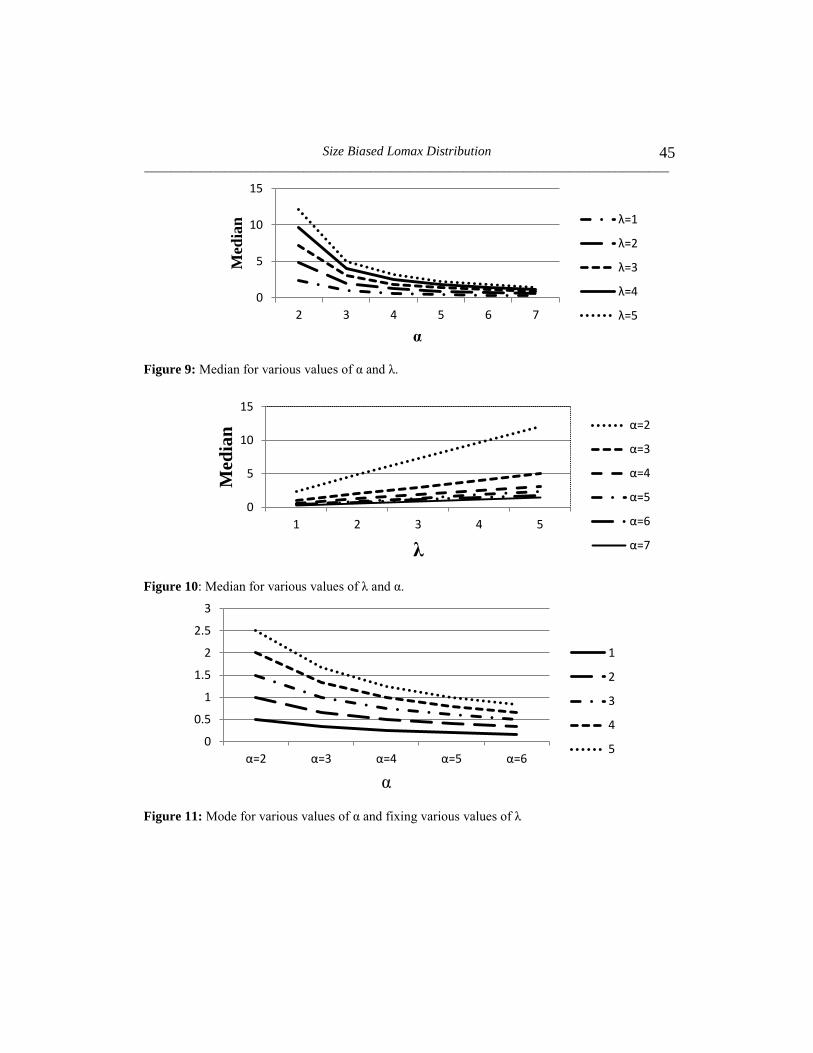
2.8 Median: Median of SBL Distribution can be obtained by solving

( ) 0.5G m

1 2 2 0m m

(2.8.1)

where,

G is the c.d.f of SBL Distribution defined in eq. (2.2).

Table 1 represents values of the median for various values of α and λ. Value of the

median decreases for increasing α when λ is fixed and opposite results are

obtained for increasing λ when α is fixed. This phenomenon is shown in the

Figure 9 and 10.

2.9 Geometric Mean:

(ln ) ln { } (E X C

where,

C is Euler Function. (2.9.1) (ln ) ( )E X CGM e e

where,

( ) ( )d

x xdx

(2.9.2)

2.10 Harmonic Mean:

1 1 (1 1)!( 1 2)!( )

( 2)!E X E

X

(2.10.1)

1

1HM

EX

(2.10.2)

2.11 Mode:

Mode is x̂

(2.11.1)

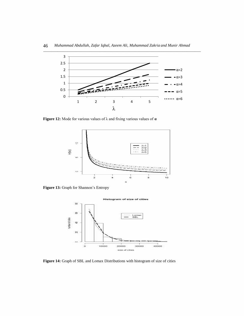
Table 2 represents values of the mode for various values of α and λ. Value of the

Mode decreases for increasing α when λ is fixed and opposite results are obtained

for increasing λ when α is fixed. One special property of this Table is that for

every value of when is fixed, increment in the value of mode is constant

(same), but fixing increasing results in decreasing the value of Mode, and

rate of decrease also decreases.


_______________________________________________________________________________ 39

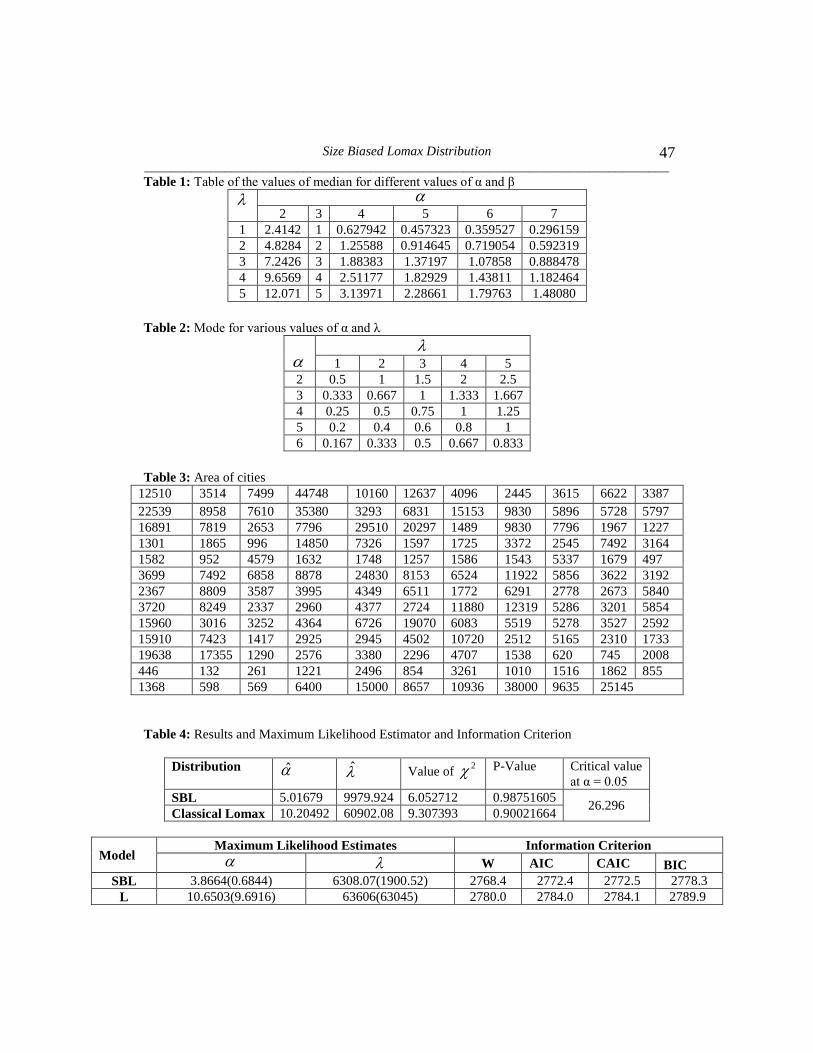
3. Entropy measures

The idea of Entropy in information theory was developed by Shannon (1948). It is

a quantitative measure of uncertainty of information related to a random

phenomenon. Like measure of dispersion, low Entropy in a Distribution indicates

more concentration and more information as compared to high Entropy. Entropy

is very useful in Reliability and Survival Analysis problems.

3.1 Shannon’s Entropy: Shannon (1948) defined Entropy as

{ ( )} [ log{ ( )}]H f x E f x

For this, SBL Distribution Shannon’s Entropy is calculated as

{ ( )} log ( 1) log ( ) ( ( 1) ( 1)H f x C

(3.1.1)

where,

C = Euler Function, 0.5772...C and ( ) ( )d

x xdx

3.2 Renyi’s Entropy: Renyi’s Entropy (1961) purposed Entropy measure as

1( ) log { ( )}

1

q

qH x f x dxq

0q and 1q

For SBL Distribution, Renyi Entropy is calculated as

1

( ) log log( ) ( 1) log log ! log( 2)! log( 1)!1

qH x q q q q q q qq

(3.2.1)

3.3 Generalized Entropy: Generalized Entropy is defined as

1( )

( 1)

vI

(Jenkins,2007)

where,

( )v x f x dx

and mean

For SBL Distribution

( 1)!

( 2)( 3)...( 3)v

and

2

2


_______________________________________________________________________________

40

1 ( 1)! 2( ) 1

( 1) ( 2)( 3)...( 3) 2I

1 ( 1)! 2( ) 1

( 1) ( 2)( 3)...( 3) 2I

,

1( 1)( ! 2

( ) 1( 3)...( 3) 2

I

, 1

(3.3.1)

4. Parameter Estimation

4.1 Estimation of parameters by Maximum Likelihood method: Probability

distribution function of SBL given by eq. (2.1) is ( )

( 1)( ) 1

x xg x

Likelihood Function is ( )

21 1

( 1)( ) 1

n n ni

i

i i

xL x

( )

1 1

log log( log log ( ) 1n n

ii

i i

xl n n n x

1

log 1n

i

i

xl n n

1

2 ni

i i

xl n

x

Putting l

and

l

equal to 0 .

1

log 1 0n

i

i

xn n

(4.1.1)

1

20

ni

i i

xn

x

1

2 ( ) 0n

i

i i

xn

x

(4.1.2)


_______________________________________________________________________________ 41

(4.1.1) and (4.1.2) are not in closed form therefore for solution we shall solve

them numerically.

4.2 Method of Moments: First sample and population moment about origin are,

'

1m X and '

1

2

By comparing both raw moment, we get,

2X

(4.2.1)

Second sample and population moment about mean are

2

2m S and 2

2 2

2

( ) ( 3)

By comparing both central moments, we get, 2

2

2

2

( ) ( )S

(4.2.2)

Solving eq. (4.2.1) and (4.2.2) 2

22

6ˆ

2

S

S X

Put in eq. (4.2.1)

22

22

ˆ

2

S XX

S X

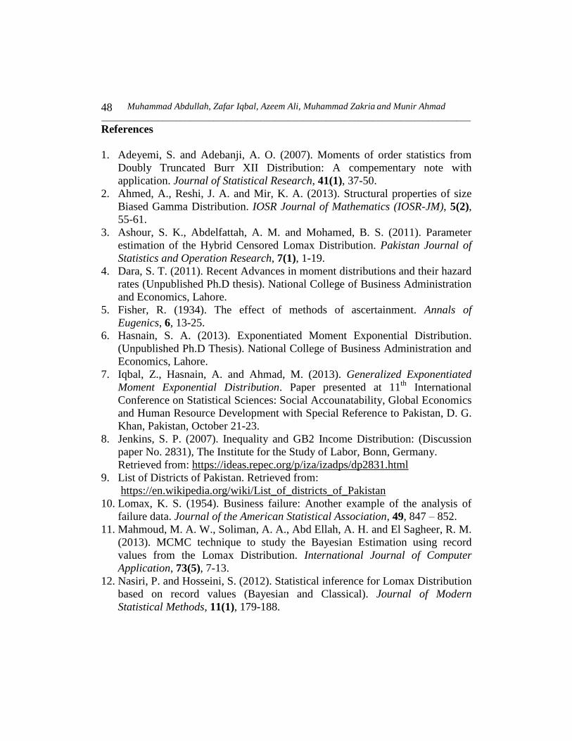
5. Application

To illustrate the performance of purposed SBL Distribution we consider the data

of size of 142 cities (Districts) including Baluchistan (31), Khyber Pakhtunkhwa

(26), Punjab (35), Sindh (20) FATA (13), Gilgit-Baltistan (7), Azad Jammun and

Kashmir (10) of Pakistan in km2 given by the website given by the website

http://en.wikipedia.org/wiki/List_of_districts_of_Pakistan, area of cities are in

Table 3.

R i386 1.3.1 is used to classify, estimate the parameters by the Method of

Moments and to find value of Chi-square statistic to compare SBL with Classical

Lomax Distribution for the above data.


_______________________________________________________________________________

42

Parameter estimates obtained from the fitting of the Size Biased Lomax

Distribution and Classical Lomax Distribution to the size of cities data in Pakistan

by Method of Moments.

Table 4 gives value of Chi-square statistics for SBL is 2 6.052712 that is less

than value of Chi-square statistic for Classical Lomax Distribution 2 9.307393 .

It means that SBL best fits the sizes of cities than Classical Lomax Distribution.

Figure 1: Size Biased Lomax for various values of α keeping λ at 1

Figure 2: Size Biased Lomax for various values of α keeping λ at 2

0 1 2 3 4

0.0

0.1

0.2

0.3

0.4

0.5

0.6

x

fx

Probabilty Distribution Plot

0 1 2 3 4 5

0.00

0.05

0.10

0.15

0.20

0.25

0.30

x

fx

Probabilty Distribution Plot

1.5, 1

2, 1

2.5, 1

3, 1

1.5, 2

2, 2

2.5, 2

3, 2


_______________________________________________________________________________ 43

Figure 3: c.d.f of SBL for different values of α keeping λ as 3 and 4.

Figure 4: Hazard Rate Function of SBL for various values of α and λ

Figure 5: Cumulative Hazard Rate Function of SBL for various values of α and λ


_______________________________________________________________________________

44

Figure 6: Survival Function of SBL for various values of α and λ

Figure 7: Skewness ( 1 ) of SBL for various values of α and λ

Figure 8: Kurtosis ( 2 ) of SBL for various values of α and λ


_______________________________________________________________________________ 45

Figure 9: Median for various values of α and λ.

Figure 10: Median for various values of λ and α.

Figure 11: Mode for various values of α and fixing various values of λ

0

5

10

15

2 3 4 5 6 7

Med

ian

α

λ=1

λ=2

λ=3

λ=4

λ=5

0

5

10

15

1 2 3 4 5

Med

ian

λ

α=2

α=3

α=4

α=5

α=6

α=7

0

0.5

1

1.5

2

2.5

3

α=2 α=3 α=4 α=5 α=6

α

1

2

3

4

5


_______________________________________________________________________________

46

Figure 12: Mode for various values of λ and fixing various values of α

Figure 13: Graph for Shannon’s Entropy

Figure 14: Graph of SBL and Lomax Distributions with histogram of size of cities

0

0.5

1

1.5

2

2.5

3

1 2 3 4 5

λ

α=2

α=3

α=4

α=5

α=6


_______________________________________________________________________________ 47

Table 1: Table of the values of median for different values of α and β

2 3 4 5 6 7

1 2.4142 1 0.627942 0.457323 0.359527 0.296159

2 4.8284 2 1.25588 0.914645 0.719054 0.592319

3 7.2426 3 1.88383 1.37197 1.07858 0.888478

4 9.6569 4 2.51177 1.82929 1.43811 1.182464

5 12.071 5 3.13971 2.28661 1.79763 1.48080

Table 2: Mode for various values of α and λ

1 2 3 4 5

2 0.5 1 1.5 2 2.5

3 0.333 0.667 1 1.333 1.667

4 0.25 0.5 0.75 1 1.25

5 0.2 0.4 0.6 0.8 1

6 0.167 0.333 0.5 0.667 0.833

Table 3: Area of cities

12510 3514 7499 44748 10160 12637 4096 2445 3615 6622 3387

22539 8958 7610 35380 3293 6831 15153 9830 5896 5728 5797

16891 7819 2653 7796 29510 20297 1489 9830 7796 1967 1227

1301 1865 996 14850 7326 1597 1725 3372 2545 7492 3164

1582 952 4579 1632 1748 1257 1586 1543 5337 1679 497

3699 7492 6858 8878 24830 8153 6524 11922 5856 3622 3192

2367 8809 3587 3995 4349 6511 1772 6291 2778 2673 5840

3720 8249 2337 2960 4377 2724 11880 12319 5286 3201 5854

15960 3016 3252 4364 6726 19070 6083 5519 5278 3527 2592

15910 7423 1417 2925 2945 4502 10720 2512 5165 2310 1733

19638 17355 1290 2576 3380 2296 4707 1538 620 745 2008

446 132 261 1221 2496 854 3261 1010 1516 1862 855

1368 598 569 6400 15000 8657 10936 38000 9635 25145

Table 4: Results and Maximum Likelihood Estimator and Information Criterion

Distribution ̂ ̂ Value of 2 P-Value Critical value

at α = 0.05

SBL 5.01679 9979.924 6.052712 0.98751605 26.296

Classical Lomax 10.20492 60902.08 9.307393 0.90021664

Model Maximum Likelihood Estimates Information Criterion

W AIC CAIC BIC

SBL 3.8664(0.6844) 6308.07(1900.52) 2768.4 2772.4 2772.5 2778.3

L 10.6503(9.6916) 63606(63045) 2780.0 2784.0 2784.1 2789.9


_______________________________________________________________________________

48

References

1. Adeyemi, S. and Adebanji, A. O. (2007). Moments of order statistics from

Doubly Truncated Burr XII Distribution: A compementary note with

application. Journal of Statistical Research, 41(1), 37-50.

2. Ahmed, A., Reshi, J. A. and Mir, K. A. (2013). Structural properties of size

Biased Gamma Distribution. IOSR Journal of Mathematics (IOSR-JM), 5(2),

55-61.

3. Ashour, S. K., Abdelfattah, A. M. and Mohamed, B. S. (2011). Parameter

estimation of the Hybrid Censored Lomax Distribution. Pakistan Journal of

Statistics and Operation Research, 7(1), 1-19.

4. Dara, S. T. (2011). Recent Advances in moment distributions and their hazard

rates (Unpublished Ph.D thesis). National College of Business Administration

and Economics, Lahore.

5. Fisher, R. (1934). The effect of methods of ascertainment. Annals of

Eugenics, 6, 13-25.

6. Hasnain, S. A. (2013). Exponentiated Moment Exponential Distribution.

(Unpublished Ph.D Thesis). National College of Business Administration and

Economics, Lahore.

7. Iqbal, Z., Hasnain, A. and Ahmad, M. (2013). Generalized Exponentiated

Moment Exponential Distribution. Paper presented at 11th

International

Conference on Statistical Sciences: Social Accounatability, Global Economics

and Human Resource Development with Special Reference to Pakistan, D. G.

Khan, Pakistan, October 21-23.

8. Jenkins, S. P. (2007). Inequality and GB2 Income Distribution: (Discussion

paper No. 2831), The Institute for the Study of Labor, Bonn, Germany.

Retrieved from: https://ideas.repec.org/p/iza/izadps/dp2831.html

9. List of Districts of Pakistan. Retrieved from:

https://en.wikipedia.org/wiki/List_of_districts_of_Pakistan

10. Lomax, K. S. (1954). Business failure: Another example of the analysis of

failure data. Journal of the American Statistical Association, 49, 847 – 852.

11. Mahmoud, M. A. W., Soliman, A. A., Abd Ellah, A. H. and El Sagheer, R. M.

(2013). MCMC technique to study the Bayesian Estimation using record

values from the Lomax Distribution. International Journal of Computer

Application, 73(5), 7-13.

12. Nasiri, P. and Hosseini, S. (2012). Statistical inference for Lomax Distribution

based on record values (Bayesian and Classical). Journal of Modern

Statistical Methods, 11(1), 179-188.

https://en.wikipedia.org/wiki/List_of_districts_of_Pakistan


_______________________________________________________________________________ 49

13. Patil, G. P. and Ord, J. K. (1976). On Size-Biased Sampling and Related

Form-Invariant Weighted Distributions. The Indian Journal of Statistics,

38(1), 48-61.

14. Rao, C. R. (1965). On discrete distributions arising out of methods of

ascertainment Classical and Contagious Discrete Distributions. Sankhya A,

(27), 311-324.

15. Renyi, A. (1961). On measures of entropy and information. In: Proceedings of

the 4th Berkeley Symposium on Mathematical Statistics and Probability, Vol.

I, University of California Press, Berkeley, 547-561.

16. Shakil, M. and Ahsanullah, M. (2012). Distributional properties of record

values of the ratio of Independent, Exponential and Gamma Random

variables. Application and Applied Mathematics: An International Journal,

7(1), 1-21.

17. Shannon, C. E. (1948). A Mathematical Theory of Communication. Bell

System Technical Journal, 27, 379–423.

Documents

Size Biased Lomax Distribution - .:.GC University Lahore 4.pdf · Size Biased Lomax Distribution Muhammad Abdullah1, Zafar Iqbal2, ... [email protected] 2 National College of Business