Six Sigma Prof. Dr. T. P. Bagchi Department of …textofvideo.nptel.ac.in/110105039/lec24.pdfSo this in fact goes on and on and on it moves like a cycle you have control then improve

Six Sigma Prof. Dr. T. P. Bagchi

Department of Management Indian Institute Of Technology, Kharagpur

Module No. # 01 Lecture No. # 24

Process Capability Good afternoon; we resume our lecture on six sigma and in particular, today’s lecture is the fourth lecture in the set of the three different other lectures that I had on statistical process control. This is the very important topic; the one that we are going to be discussing today this is called process capability as you see in the slide. There the title slide it talks about the capability of the process to be able to satisfy customer requirements; that is what basically this is.

(Refer Slide Time: 00:44)


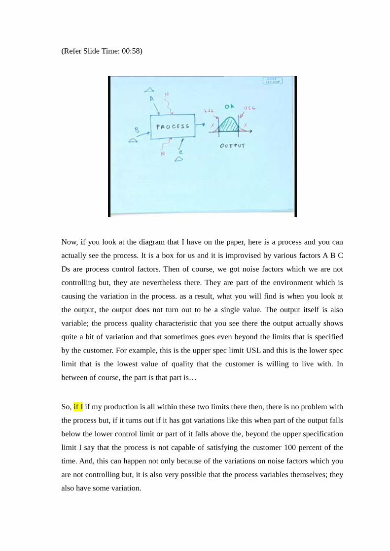
Now, if you look at the diagram that I have on the paper, here is a process and you can

actually see the process. It is a box for us and it is improvised by various factors A B C

Ds are process control factors. Then of course, we got noise factors which we are not

controlling but, they are nevertheless there. They are part of the environment which is

causing the variation in the process. as a result, what you will find is when you look at

the output, the output does not turn out to be a single value. The output itself is also

variable; the process quality characteristic that you see there the output actually shows

quite a bit of variation and that sometimes goes even beyond the limits that is specified

by the customer. For example, this is the upper spec limit USL and this is the lower spec

limit that is the lowest value of quality that the customer is willing to live with. In

between of course, the part is that part is…

So, if I if my production is all within these two limits there then, there is no problem with

the process but, if it turns out if it has got variations like this when part of the output falls

below the lower control limit or part of it falls above the, beyond the upper specification

limit I say that the process is not capable of satisfying the customer 100 percent of the

time. And, this can happen not only because of the variations on noise factors which you

are not controlling but, it is also very possible that the process variables themselves; they

also have some variation.

So each of the process variables that you set at the set point they may also have some

variation and because of that these variations they impact the process and the result is

you got some inflated variation in the output of the process itself. Process capability: this

phrase is the measure of, how will a particular process be able to satisfy or fall within the

upper and lower specification in this? That is what really process capability is to.


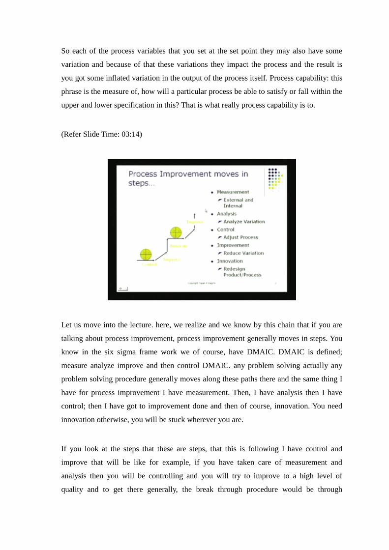
Let us move into the lecture. here, we realize and we know by this chain that if you are

talking about process improvement, process improvement generally moves in steps. You

know in the six sigma frame work we of course, have DMAIC. DMAIC is defined;

measure analyze improve and then control DMAIC. any problem solving actually any

problem solving procedure generally moves along these paths there and the same thing I

have for process improvement I have measurement. Then, I have analysis then I have

control; then I have got to improvement done and then of course, innovation. You need

innovation otherwise, you will be stuck wherever you are.

If you look at the steps that these are steps, that this is following I have control and

improve that will be like for example, if you have taken care of measurement and

analysis then you will be controlling and you will try to improve to a high level of

quality and to get there generally, the break through procedure would be through

innovation. That would come through a process like design of experiments for example,

and again you would stabilize with your PDCA cycle. You stabilize around a certain

level of quality; from there you might like to compete a bit better and you would like to

improve the process and that you do.

So this in fact goes on and on and on it moves like a cycle you have control then improve

innovate then again control improve innovate and so on. That is how you will be moving

along one of the reasons for doing this is generate to try to improve the process

capability of any process that you are operating. If you are not doing it your competition

for sure is doing it this competition generally a good competitive he benchmarks is

products against the best that is there in the market place and it tries to offer value. Value

is what you offers for the price that you offer in you will always try to improve upon the

value that is offering and he’d like to he try his best to try to out compete other people.


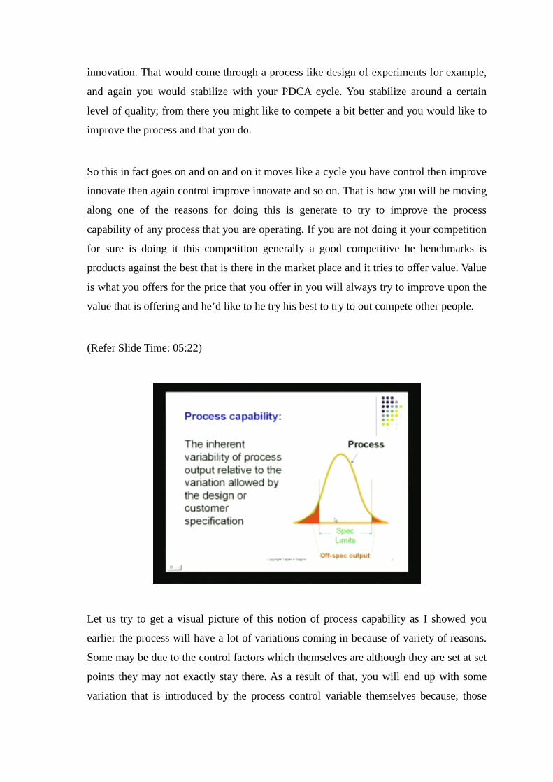
Let us try to get a visual picture of this notion of process capability as I showed you

earlier the process will have a lot of variations coming in because of variety of reasons.

Some may be due to the control factors which themselves are although they are set at set

points they may not exactly stay there. As a result of that, you will end up with some

variation that is introduced by the process control variable themselves because, those

themselves they did not hold on to their set points. Then of course, in addition we have to

other factor that you are not controlling and these are the noise factors as you saw in the

diagram there is a noise factor here and there is a noise factor here and these are all

operating independent of whatever else is going on there.

So, they will also be active and they will also try to impact the variability of the process

itself. When that happens, return into the slide there the screen here we have where we

end up with what we call some inherent variability of the process. we realize that every

process is going to be variable. Unfortunately, what happens, customers as customers we

have our specific requirement and these specific requirements are communicated and

they are actually captured by market research and those would be called what we call

specification limits. This is kind of the tolerance band within which the product would be

treated to be and if it goes beyond that tolerance band the product would be considered to

be off spec. That is exactly what we see there, when we look at the output there these red

regions. These two red regions one is to the left the other is to the right these two indicate

basically the different points which are below either below these specification limit or

above the specification limit. These products if they are offered in the market price no

one is going to buy them because, they are beyond the specification limit that is

something you got to remember. Therefore, it becomes very important for us to worry

about a process that is delivering products that fall beyond these specification limits; they

are below the lower specification limit or above the upper specification limit it is very

important that we design processes and operate them in a manner that keeps the total

process inside this specification limits all the time. Such a process will be called a

capable process; if a process goes as it is operating naturally, if it goes if it produces

output that goes beyond the upper and lower specification limits, we will say that the that

particular process is not capable.


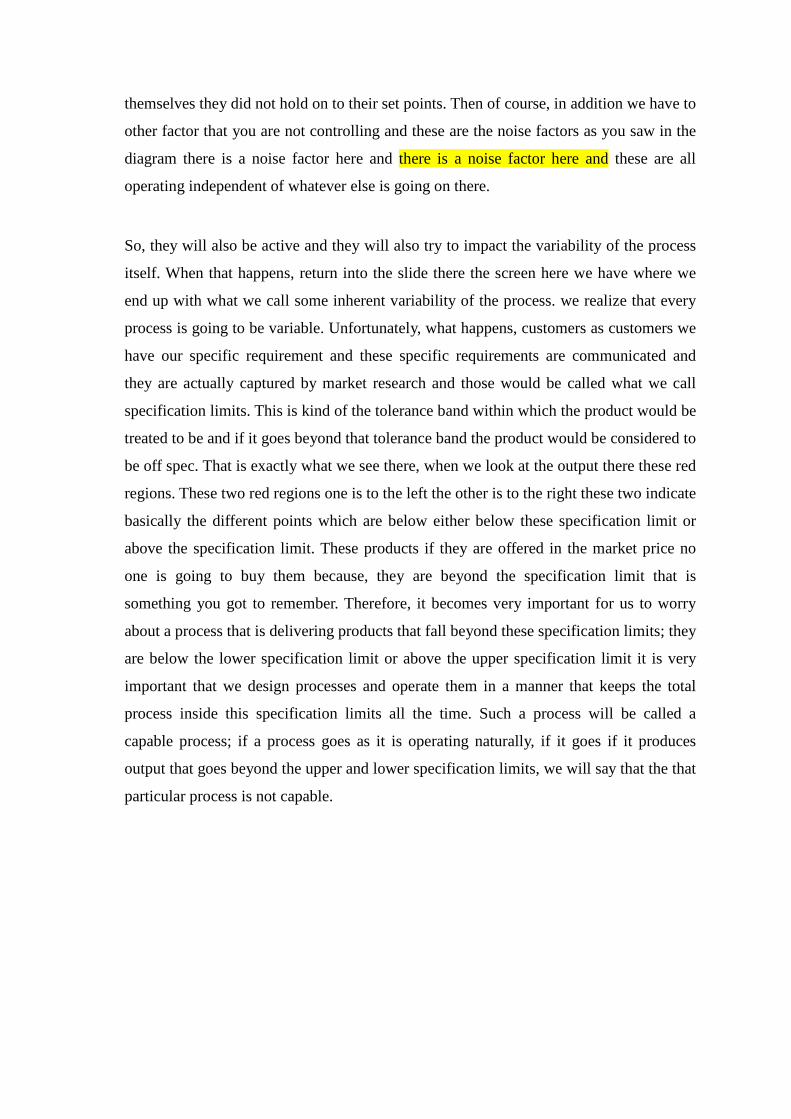
We will try some quantitative measures of this as you go into this; what does process

capability analysis do? It actually focuses on improvement it tries to improve process

capability of a particular process. Any process that you bring about it will always have

some variation. What we have to do is we have to make sure that that variation does not

take the output beyond these specification limits.

Now, such a process will generally be under the influence of factors which cause too

much variation. One of the task in process capability analysis is first of all to obtain a

measure of how good that presents as this, as this capability is if that turns out to be too

large. If it turns out that there are parts of process that are producing output which are

going beyond these specification limits; we have to tighten the process that means, we

have to go back.

If you look at the procedure diagram, in this diagram there are these factors A B and C.

perhaps, they have been set in such a way or process on them are not good enough to

keep this process well within the specification limit. When you would look at the output

of the process perhaps there are too much variations in these and perhaps there is too

much noise. Also, these are the reasons why my output may be beyond the specification

limits and my process capability may be poor in trying to measure in trying to quantify

process capability.

What we do is, we will look at the individual output values. We look at the individual

output values; so perhaps for example, it could be the x 1 x 2 x 3. These are

measurements produced that are coming out that are on the items that are coming of the

production line you measure some quality dimension it could be distance and it could be

length, it could be weight, it could be viscosity. It could be any of these things; any of

these characteristics that you can measure. Once you measured it you go out here and

you compare that quantity; you compare that quantities, value to the tolerance if it turns

out that the measured value is beyond the tolerance. That means, you produce something

that is off spec which we call in industry, we call it off spec.

Our goal is going to be to try to understand factors that are causing this wide variation in

the process and are producing products that are beyond this specification limits. So, the

process capability study is actually they really look at the range of the individual outputs.

In fact, the output that I show here the output that I show here these are the plots of the

individual items. So, I have got various individual items they have been plotted on this

and it turns out some of those are below the specification limit here on the lower side and

some are beyond the upper specification limit but, these are all individual measurements.

I am not talking about x bar, I am not talking about r; I am talking about raw x values

that is what I am talking about. That is what I have plotted; in fact, that is the quantity

that I need to measure in large quantities large numbers to try to see what that

distribution looks like.

If that distribution turns out to be (()) and a lot of good junk of it is beyond these

specification limit, I will say that the process is not capable. I cannot go out to the market

place and compete in the market place in the open market place with a process which is

producing products that are generally off spec and that are good fraction of this

production that is off spec in trying to measure process capability. We make an

assumption, we assume that the output is going to be normal of course, we could work

with any other distribution but, the convention has been that we have assume the output

to be normal.

In fact, most of the stuff if you measure them if you look at measured data measured data

generally follows the normal distribution that just makes our life little easier when it

comes to quantifying process capability the other thing that we would also like is we

would like the process to be under the influence of chance cause on their we do not want

the assignable factors to be disturbing the process when I am trying to make a

measurement of a process capability.

So when I think of measuring process capability, it is very important for us to realize that

the process must be under what we call statistical control. That means, it is under the

influence of the ( )… are small vibrations and so on and so forth. Those are the parts;

those are the causes which do not shake the process too much. Any factor, any item, any

cause that are actually would shake the process we first have to stabilize the process. We

first have to make sure we have removed all the assignable factors and the way to do that

is run the process under the process control using control charts. Perhaps, the x bar chart

or the r chart and then remove as many of those factors as possible. Once you have done

that what is left is the process that is operating under the influence of chance causes on

their…


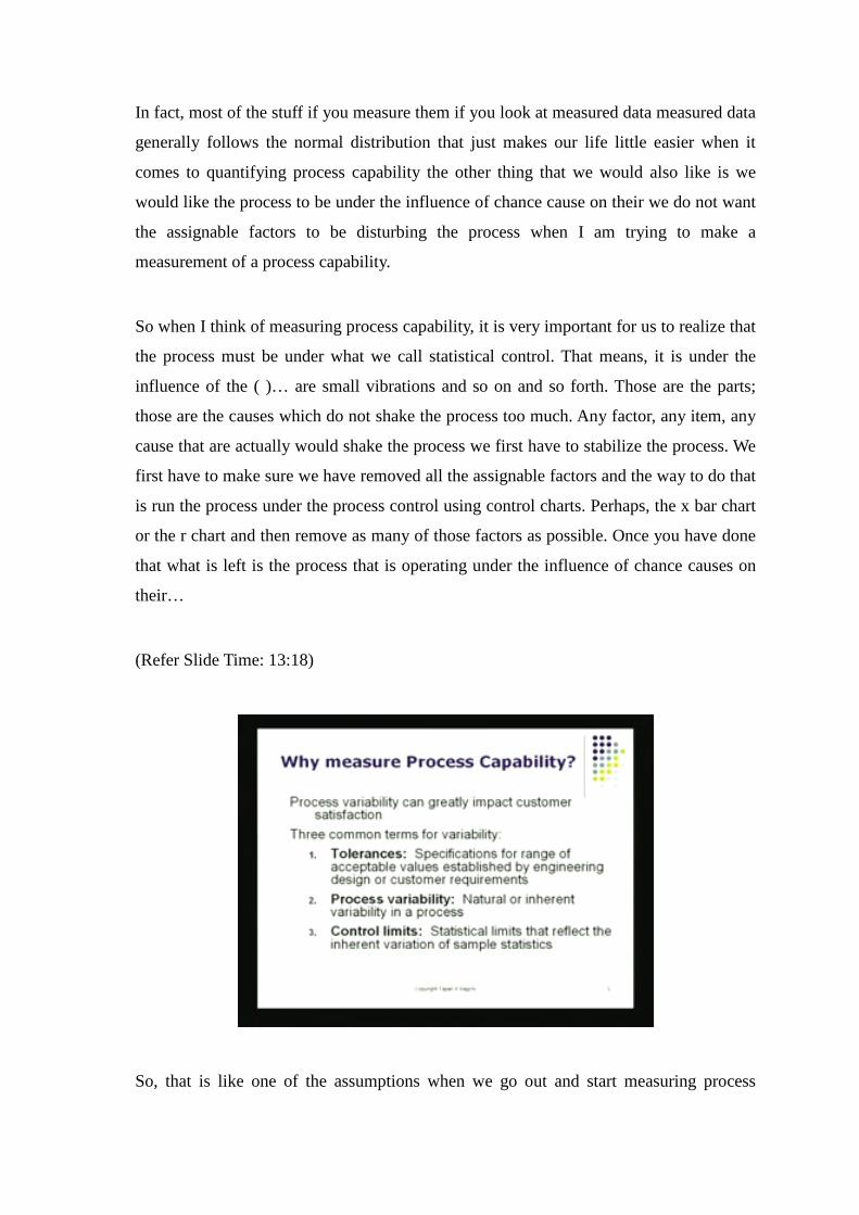
So, that is like one of the assumptions when we go out and start measuring process

capability, couple of terms we will be using here. One is of course, tolerance and

tolerance is the difference between the upper and lower spec limit and if you look at my

diagram here, these specification limits here is denoted by this line there. That is the

upper spec limit and this is the lower spec limit. This range is the tolerance; this actually

implies the range of quality characteristic values that the customer is willing to live with

this is rather important for us to realize we got to find out what that tolerance is that is

given by the customer the second thing of course, is the variability and again you can

notice the variability there that is a notion of touch really. Basically, the plotting of all the

output that I have measured without controlling anything, without basically doing any

kind of screening and any kind of censoring and so on; we just take that raw data and we

plot them up completely and that would reflect now. The variability in the procedure

itself that is also (()) very important; we got to remember now whenever we are dealing

with process capability we are going to be using specification limits not control limits.

So, yes we use control limits to stabilize the process we use control limits on control

charts to try to stabilize the process which means, we want to remove any assignable

cause that might be disturbing the process. That is something we would like to be able to

do but, once we done that the process capability measurement will in no place utilize

control limits that it will not do. So, please do not be confuse between these two types of

limit one is specification limits these basically specify the range or the tolerance that the

customer is willing to live with that is the range of quality characteristics that is

acceptable to the customer. On the other hand, if I am trying to control the process, if I

am trying to do control using statistical process control, I shall be interested in what we

call control limits. Then, these control limits would be imposed on these two statistical

charts one is the x bar chart; the other is the r chart when I am making measurements. I

could do of course, the same thing with p chart or c chart any of those charts but, is use

control limits only to stabilize the process only to bring it under what we call statistical

control.


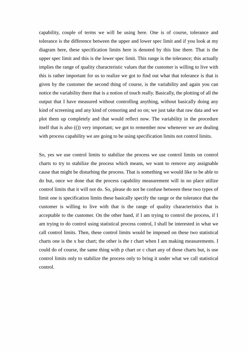
Let us go on and take a look at the distribution itself. Here is the distribution and if you

remember the normal distribution, the normal distribution is symmetric, has got two

parameters controlling it. One is mu which shows the mean of the process; the other is

sigma. Sigma indicates the variability of the process; so, there are two aspects of the

output here. One is of course, where it is located central where is the central location of

the process there is a central point about which the process data are distributed.

So, that is going to be our mu; the mean then of course, we also have to bring in what we

call variability of the process and the parameter that indicates that very easily is our

sigma - sigma is standard deviation and if you specify mu and sigma you defined

everything that you need when it comes to defining a the normal distribution. Now, some

other some other features also we utilize, now once we have acknowledge that the

process is going to be normal distribution, normally distributed. We do a couple of things

we can mark parts that will specify the exact area the exact area that will fall within a

certain range that is beyond, that is above and below the mean value of the thing.

If I go 1 sigma beyond mu that is like this point is now going to be mu plus 1 sigma and

this point is going to be mu minus 1 sigma this difference here the distance between

these two is 2 sigma and that covers approximate 68 percent of production. If your

output is going to be normally distributed; if it is normally distributed then within plus

sigma and minus sigma you will have 68 percent of production. If you go beyond this if

you go to 2 sigma limit on the right hand side and 2 sigma below the average below the

mean there that will cover about 95 percent of the total area that is under the distribution;

that is the distribution of the output that is there if the output is normally distributed.

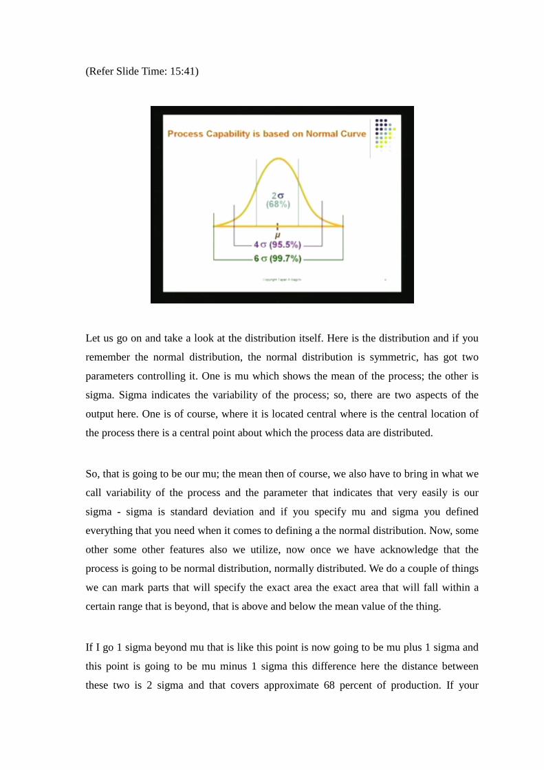
If you go to 3 sigma, the range that is covered between mu plus 3 sigma and mu minus 3

sigma that total area turns out to be 99.7 percent. So, very little is left beyond that. In

fact, these turn out to be measures that we utilize when we do our process capability

calculations. So, mething for us to remember is if the distribution is normal then within

plus and minus 1 sigma i will have 68 percent of the output. If I expand that range to plus

and minus 2 sigma i will have 95 percent production that will be in that range that mu

range plus minus 2 sigma and if I make that tolerance even wider if I make it 3 sigma

that is if I go mu plus 3 sigma would be the upper limit and mu minus 3 sigma will be the

lower limit. Then, the amount of output that is inside the plus 3 sigma and minus sigma

range that is going to be 99.7 percent this is the property above the normal distribution.

This is the property of the normal distribution and we utilize this when we do our C pk

calculations.


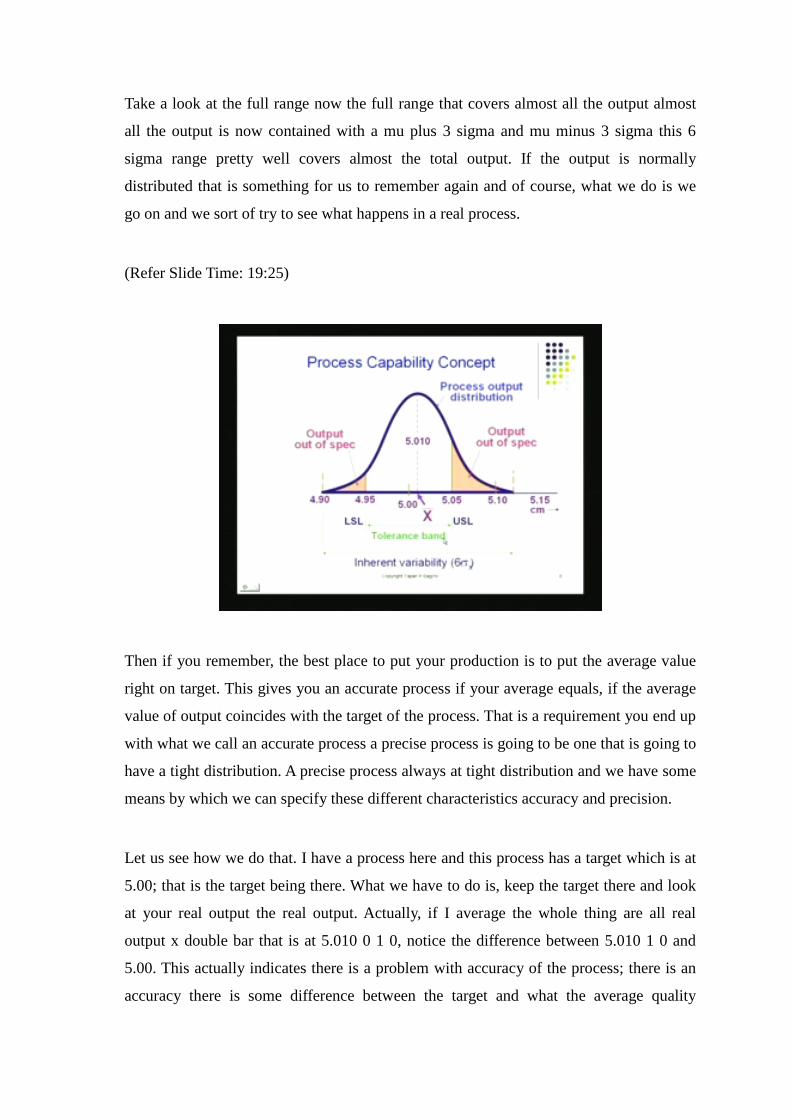
Take a look at the full range now the full range that covers almost all the output almost

all the output is now contained with a mu plus 3 sigma and mu minus 3 sigma this 6

sigma range pretty well covers almost the total output. If the output is normally

distributed that is something for us to remember again and of course, what we do is we

go on and we sort of try to see what happens in a real process.


Then if you remember, the best place to put your production is to put the average value

right on target. This gives you an accurate process if your average equals, if the average

value of output coincides with the target of the process. That is a requirement you end up

with what we call an accurate process a precise process is going to be one that is going to

have a tight distribution. A precise process always at tight distribution and we have some

means by which we can specify these different characteristics accuracy and precision.

Let us see how we do that. I have a process here and this process has a target which is at

5.00; that is the target being there. What we have to do is, keep the target there and look

at your real output the real output. Actually, if I average the whole thing are all real

output x double bar that is at 5.010 0 1 0, notice the difference between 5.010 1 0 and

5.00. This actually indicates there is a problem with accuracy of the process; there is an

accuracy there is some difference between the target and what the average quality

characteristic is that the process is delivering. So, here the first problem that we have is

we have a some problem of accuracy. Then of course, there is something that I would

like to find out from customers and I say regardless of whatever the process is doing

what are your requirements. Then, the customer comes along he says well the target is

correct I want the quality characteristic to have the value of 5.00; my tolerance on the

upper side is 5.0 5 and my tolerance on the lower side is 4.95 and that is going to be my

tolerance value. if you supply output if I supply products that are in this range, I will be

pretty happy.

Of course, I will be most happy if you supply it right of the target but, I tolerate things

that are I will accept things that fall within the upper spec limit and lower spec limit and

this is my tolerance band; this would the customer conveys to you. Now, come back to

production come back to the process remember the process that I showed I showed you a

process when I drew the diagram here is a process the process is what I am operating I

will manufacture I am operating this process my output may not exactly we fit for the

customer to use one hundred percent of the time. Let us take a look at what is happening

there the target has been given as 5.00 and the tolerance band has been given as 4.95 to

5.05; these have come from the customer.

When I collect some output data and I plot, it gives me this dark curve there which is you

can recognize it is a normal distribution; more or less a normal distribution alone. They

hold a good junk of that normal distribution it falls below the lower specification limit so

this would be call out of specification these products are going to be out of specification

these would not be acceptable to the customer if I look at the outside if I look at beyond

the upper spec limit again I find there is a whole bunch of output there that is again

beyond the beyond the tolerance of the customer.

So again, these are again out of spec; if a lot of my production is like this and this I

cannot compete in the market place with the process that I have that is operating like this

and that actually means that the process capability of this process. This blue process of

this dark blue process is not so good, is actually not so good it turns out that the inherent

variability this is the natural variability of process that is wider than the tolerance band.

Therefore, in the language of process capability the process is not capable of taking care

of the customer requirements 100 percent it is not.


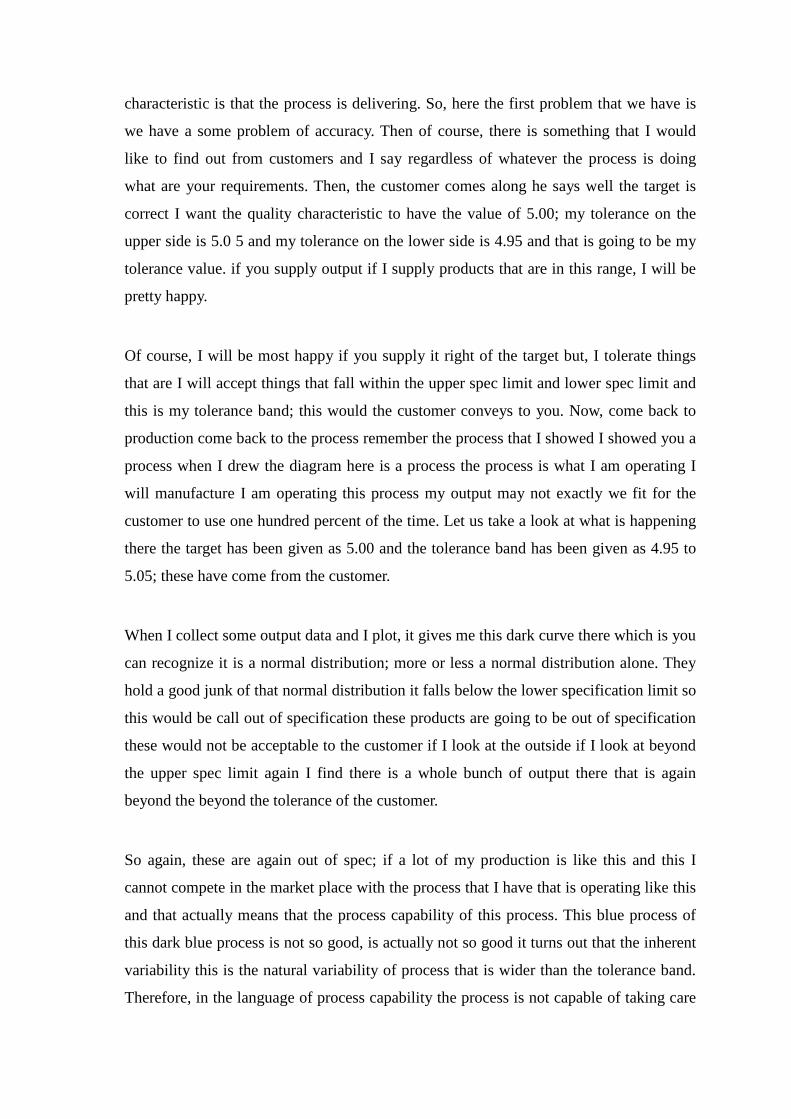
Let us take a look at two processes; one is a perfect process. I show the tolerance here the

upper and lower specification limits and look at the natural variation of the output its

well within the tolerance. So, this is the good process this is what we call capable process

it is only within the tolerance the natural variation of this process is only within the

tolerance look at this process by contrast the tails are beyond the tolerance limits which

actually says if I use this process to basically support by a market place, there will be

many occasions when there will be complaints from the customer because I find some

tails of it that are beyond the beyond the tolerance limits and this process is therefore, not

capable.

So the green process is capable but, this lower process is not capable this is just a give

you an idea of what we are talking about when talk of capability the process to be

capable has to be wholly within the tolerance the same picture is shown here.


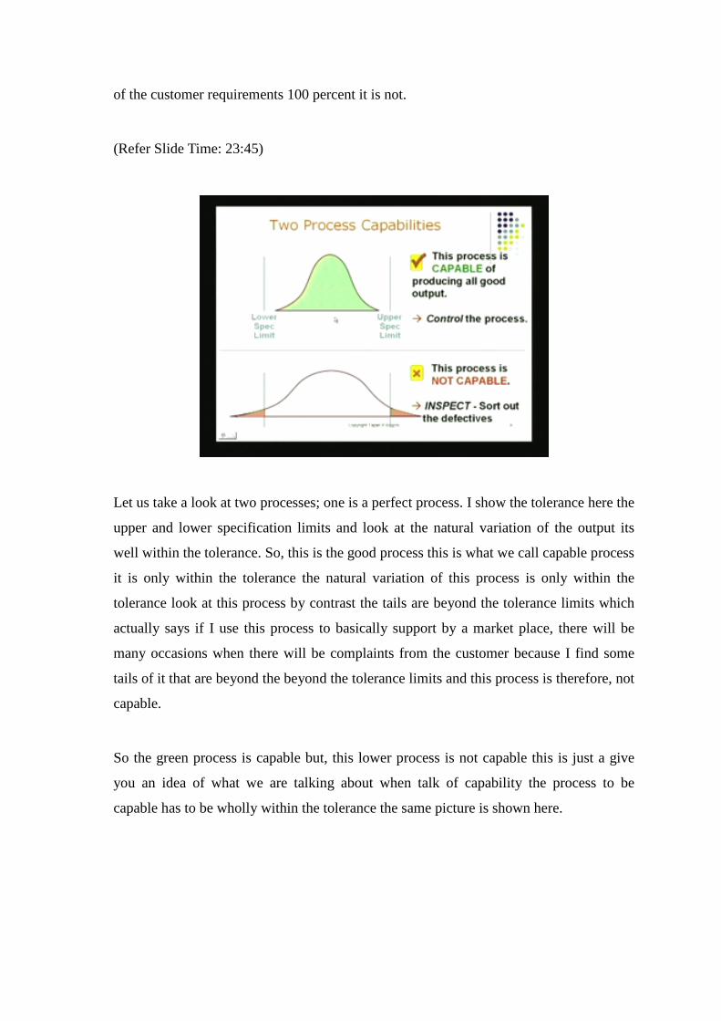
Now, what do we do? What can we do if we got a process like this? This is the process

that again is as you can see right away - the lower and upper specification limits are

shown and there are red tails which are like unacceptable out there what do we do well

we could redesign the process we could change those factors A B and C. Remember,

these factors A B and C? These are process control factors perhaps also there is a lot of

noise that is causing the inherent variation plus, we could redesign this process we could

probably redesign this process and bring it wholly within the tolerance limits and the

tolerance limits as indicated to you those are shown right there.

That could be done by redesigning the process; that would be one strategy. Suppose, this

was the machine that was like an old machine and there is no way I can redesign or I can

fix the machine then of course, I will have to go for alternate process that is like another

option that is option number 2. That is also a possibility if I am going to be competing at

the same market place; that is also going to be one of my one of my requirements I shall

be using an alternate process to supply into this market place. The third approach is

going to be why do not why produce the way I produce? But, I sort the output between

good and bad what I do is I make some deliver inspection I inspect everything that

comes out of the process and I reject the parts from shipment that are either below the

lower specification limits or above the upper specification limit. I supply parts or I

supply products that only fall within the tolerance band and throw away the parts.

Perhaps, I scrap the part or I rework the parts that are beyond this spec limit; that is going

to be expensive again. And, the other thing of course, is I go and plead with the customer

please widen your tolerance band if I did that with the process that I have here if the

customer is kind enough if he would widen the tolerance band then these red area will

reduce in size that could be my four strategies certainly not a good strategy at all the best

strategy is really to redesign the process and that means you have to identify factors

which are causing this wide variability.


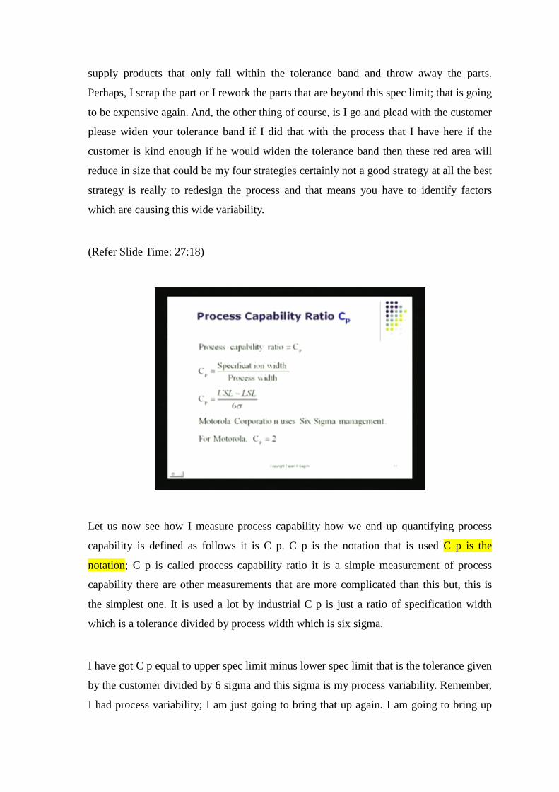
Let us now see how I measure process capability how we end up quantifying process

capability is defined as follows it is C p. C p is the notation that is used C p is the

notation; C p is called process capability ratio it is a simple measurement of process

capability there are other measurements that are more complicated than this but, this is

the simplest one. It is used a lot by industrial C p is just a ratio of specification width

which is a tolerance divided by process width which is six sigma.

I have got C p equal to upper spec limit minus lower spec limit that is the tolerance given

by the customer divided by 6 sigma and this sigma is my process variability. Remember,

I had process variability; I am just going to bring that up again. I am going to bring up

this is my notice here. The 6 sigma limit there this is my process variability. So, this

would be in my denominator when I look at my C pk formula. My C p formula gives me

6 sigma in the denominator; I have got tolerance of these are numerator and I have got in

the denominator I have got six sigma this ratio would be called C p. It turns out if a

process is six sigma process then your process has such good precision and your

centering is so good that this C p number turns out to be 2 for your process. Let me give

you one or two other examples.


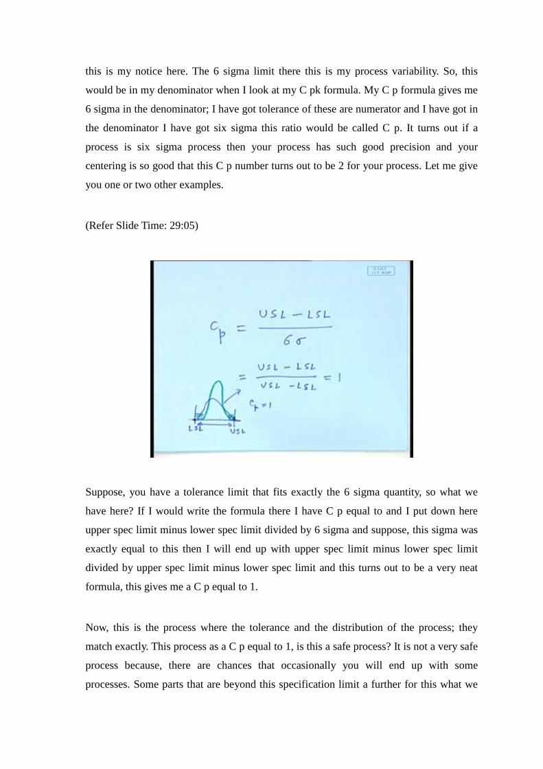
Suppose, you have a tolerance limit that fits exactly the 6 sigma quantity, so what we

have here? If I would write the formula there I have C p equal to and I put down here

upper spec limit minus lower spec limit divided by 6 sigma and suppose, this sigma was

exactly equal to this then I will end up with upper spec limit minus lower spec limit

divided by upper spec limit minus lower spec limit and this turns out to be a very neat

formula, this gives me a C p equal to 1.

Now, this is the process where the tolerance and the distribution of the process; they

match exactly. This process as a C p equal to 1, is this a safe process? It is not a very safe

process because, there are chances that occasionally you will end up with some

processes. Some parts that are beyond this specification limit a further for this what we

have to do is, we have to make this tighter. So, we should in fact try to get a process. We

should understand the causes of variation; we should try to get a process that is wholly

within the limits like this. So, there is some room here and also there is some room here;

so, real danger of going beyond the control, beyond the specification limits, I have the

upper specification limit here, upper specification limit there and lower specification

limit there. Those are my my tolerance band; this is my tolerance band and of course,

then within that my good process is such is got some slack left on both sides.

So that, this one is really it has it has hardly any chance of going beyond these lower and

upper specification limit in Motorola’s case when they reached there, when they

produced a process that had a 6 sigma of quality. That means, it produces part that was

only 3 or 4 part per million; their C p measured turns out to be 2 turn out to be 2.


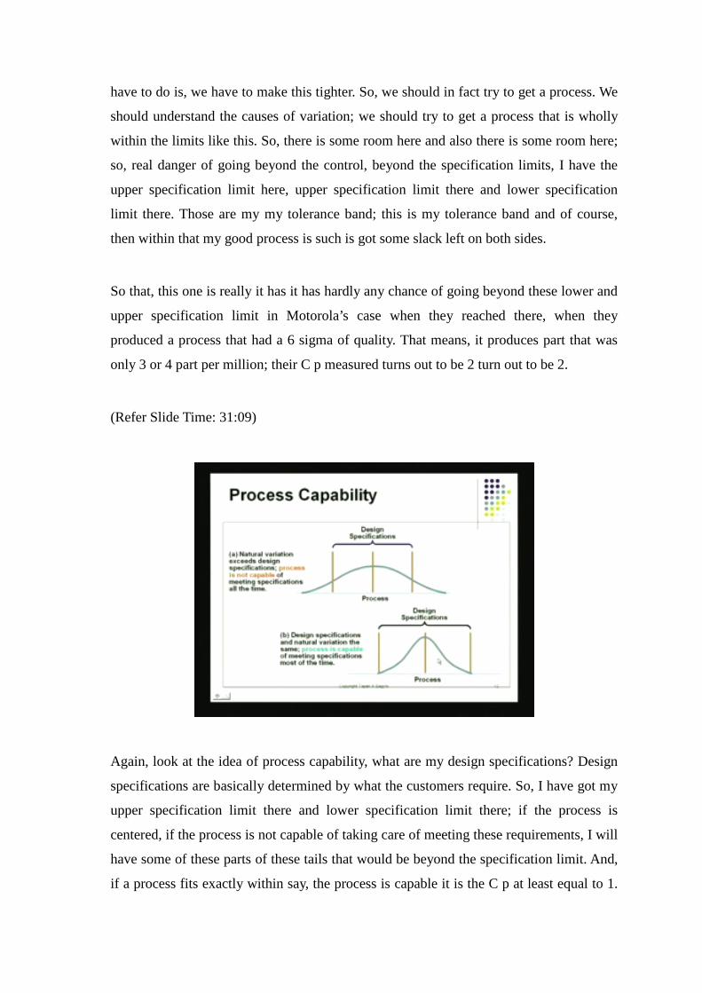
Again, look at the idea of process capability, what are my design specifications? Design

specifications are basically determined by what the customers require. So, I have got my

upper specification limit there and lower specification limit there; if the process is

centered, if the process is not capable of taking care of meeting these requirements, I will

have some of these parts of these tails that would be beyond the specification limit. And,

if a process fits exactly within say, the process is capable it is the C p at least equal to 1.

Hopefully, it should have C p that is more than 1 is always greater and certainly below 1

is not acceptable.


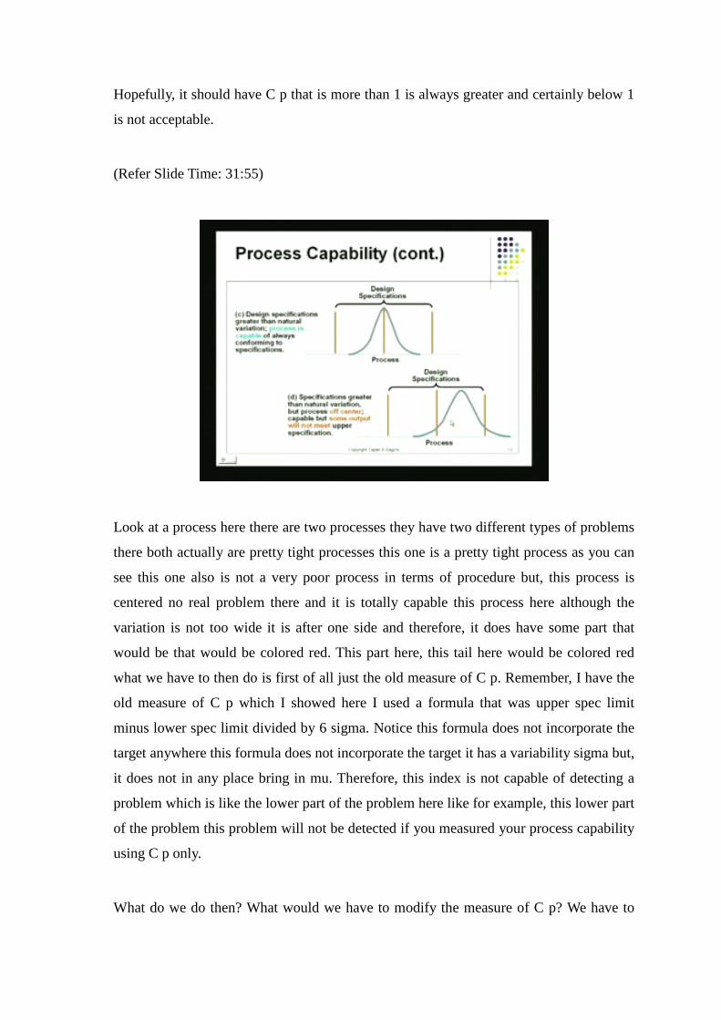
Look at a process here there are two processes they have two different types of problems

there both actually are pretty tight processes this one is a pretty tight process as you can

see this one also is not a very poor process in terms of procedure but, this process is

centered no real problem there and it is totally capable this process here although the

variation is not too wide it is after one side and therefore, it does have some part that

would be that would be colored red. This part here, this tail here would be colored red

what we have to then do is first of all just the old measure of C p. Remember, I have the

old measure of C p which I showed here I used a formula that was upper spec limit

minus lower spec limit divided by 6 sigma. Notice this formula does not incorporate the

target anywhere this formula does not incorporate the target it has a variability sigma but,

it does not in any place bring in mu. Therefore, this index is not capable of detecting a

problem which is like the lower part of the problem here like for example, this lower part

of the problem this problem will not be detected if you measured your process capability

using C p only.

What do we do then? What would we have to modify the measure of C p? We have to

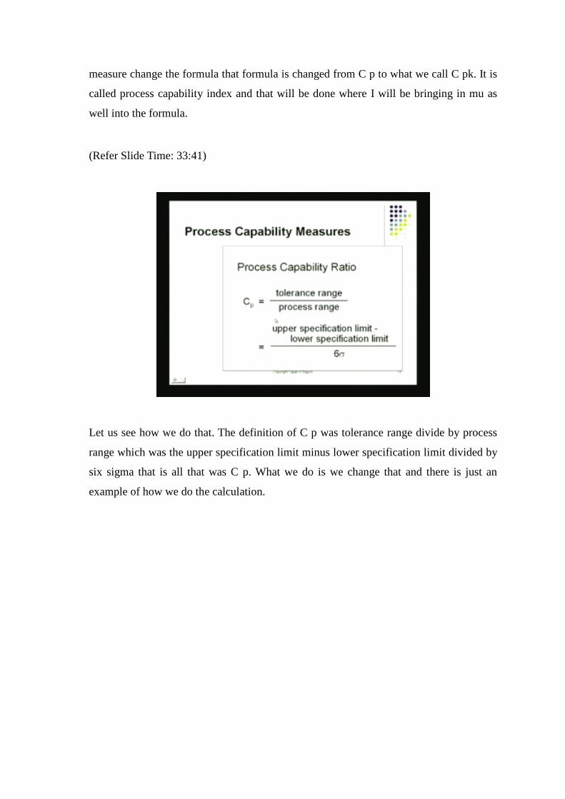
measure change the formula that formula is changed from C p to what we call C pk. It is

called process capability index and that will be done where I will be bringing in mu as

well into the formula.


Let us see how we do that. The definition of C p was tolerance range divide by process

range which was the upper specification limit minus lower specification limit divided by

six sigma that is all that was C p. What we do is we change that and there is just an

example of how we do the calculation.


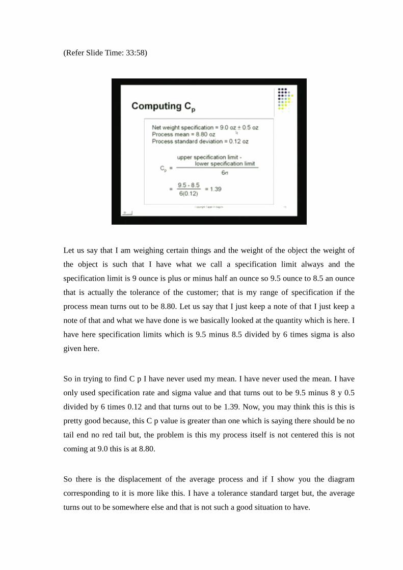
Let us say that I am weighing certain things and the weight of the object the weight of

the object is such that I have what we call a specification limit always and the

specification limit is 9 ounce is plus or minus half an ounce so 9.5 ounce to 8.5 an ounce

that is actually the tolerance of the customer; that is my range of specification if the

process mean turns out to be 8.80. Let us say that I just keep a note of that I just keep a

note of that and what we have done is we basically looked at the quantity which is here. I

have here specification limits which is 9.5 minus 8.5 divided by 6 times sigma is also

given here.

So in trying to find C p I have never used my mean. I have never used the mean. I have

only used specification rate and sigma value and that turns out to be 9.5 minus 8 y 0.5

divided by 6 times 0.12 and that turns out to be 1.39. Now, you may think this is this is

pretty good because, this C p value is greater than one which is saying there should be no

tail end no red tail but, the problem is this my process itself is not centered this is not

coming at 9.0 this is at 8.80.

So there is the displacement of the average process and if I show you the diagram

corresponding to it is more like this. I have a tolerance standard target but, the average

turns out to be somewhere else and that is not such a good situation to have.

Let us see what we do perhaps, what we should do is instead of misleading management

by calculating only C p. We got to convey to them look gentlemen, there is a difference

between the process mean that is being delivered by the process and what we consider to

be that is the target that is really the best value of the quality characteristic. That is

required by the customer to do this what we do is we change the formula we calculate

process capability.


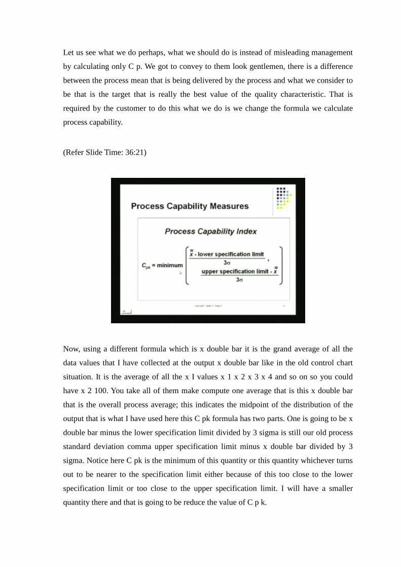
Now, using a different formula which is x double bar it is the grand average of all the

data values that I have collected at the output x double bar like in the old control chart

situation. It is the average of all the x I values x 1 x 2 x 3 x 4 and so on so you could

have x 2 100. You take all of them make compute one average that is this x double bar

that is the overall process average; this indicates the midpoint of the distribution of the

output that is what I have used here this C pk formula has two parts. One is going to be x

double bar minus the lower specification limit divided by 3 sigma is still our old process

standard deviation comma upper specification limit minus x double bar divided by 3

sigma. Notice here C pk is the minimum of this quantity or this quantity whichever turns

out to be nearer to the specification limit either because of this too close to the lower

specification limit or too close to the upper specification limit. I will have a smaller

quantity there and that is going to be reduce the value of C p k.


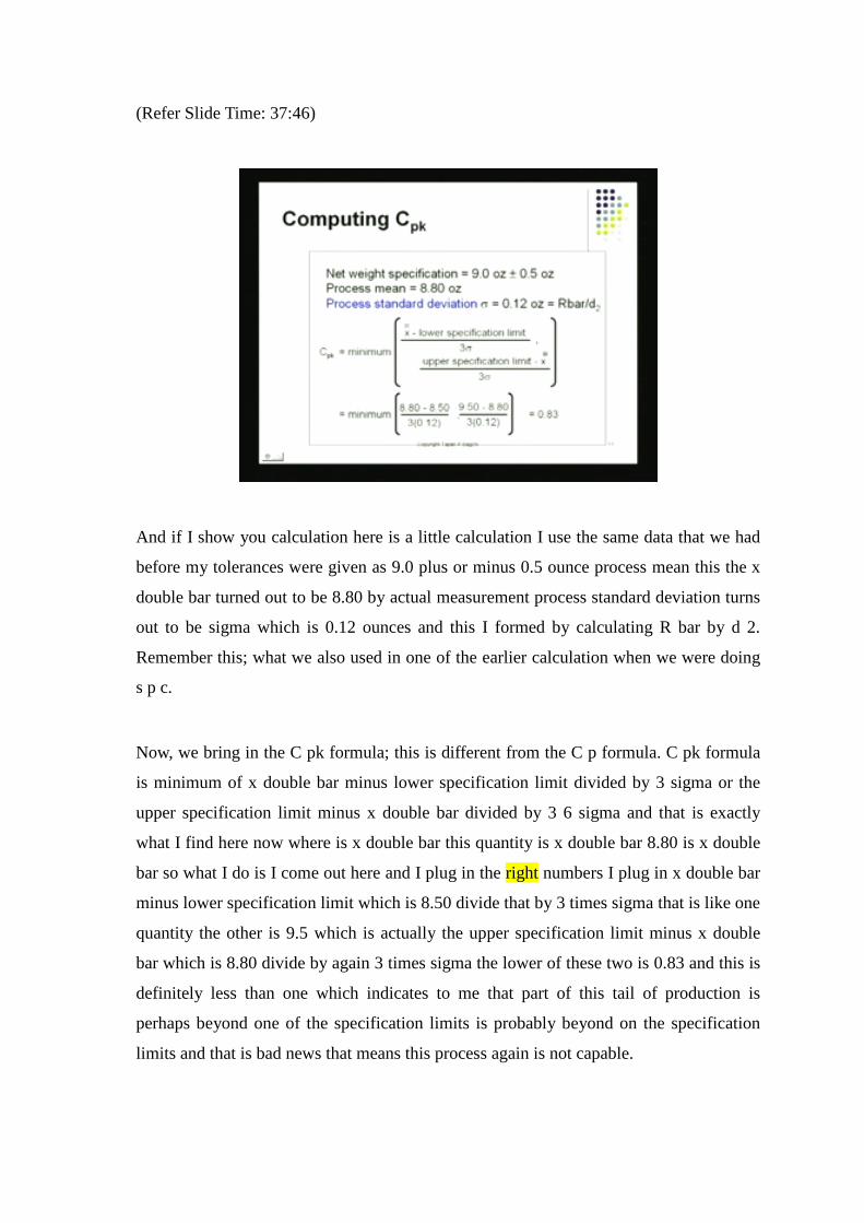
And if I show you calculation here is a little calculation I use the same data that we had

before my tolerances were given as 9.0 plus or minus 0.5 ounce process mean this the x

double bar turned out to be 8.80 by actual measurement process standard deviation turns

out to be sigma which is 0.12 ounces and this I formed by calculating R bar by d 2.

Remember this; what we also used in one of the earlier calculation when we were doing

s p c.

Now, we bring in the C pk formula; this is different from the C p formula. C pk formula

is minimum of x double bar minus lower specification limit divided by 3 sigma or the

upper specification limit minus x double bar divided by 3 6 sigma and that is exactly

what I find here now where is x double bar this quantity is x double bar 8.80 is x double

bar so what I do is I come out here and I plug in the right numbers I plug in x double bar

minus lower specification limit which is 8.50 divide that by 3 times sigma that is like one

quantity the other is 9.5 which is actually the upper specification limit minus x double

bar which is 8.80 divide by again 3 times sigma the lower of these two is 0.83 and this is

definitely less than one which indicates to me that part of this tail of production is

perhaps beyond one of the specification limits is probably beyond on the specification

limits and that is bad news that means this process again is not capable.

So notice the difference in going from C p to C pk C p basically looks at the overall

variability of the process C pk looks at the centrality of the process C pk worries about

the displacement of the overall average from the targeted value that is what C pk does so

C pk turns out to be a better value for measuring process capability.


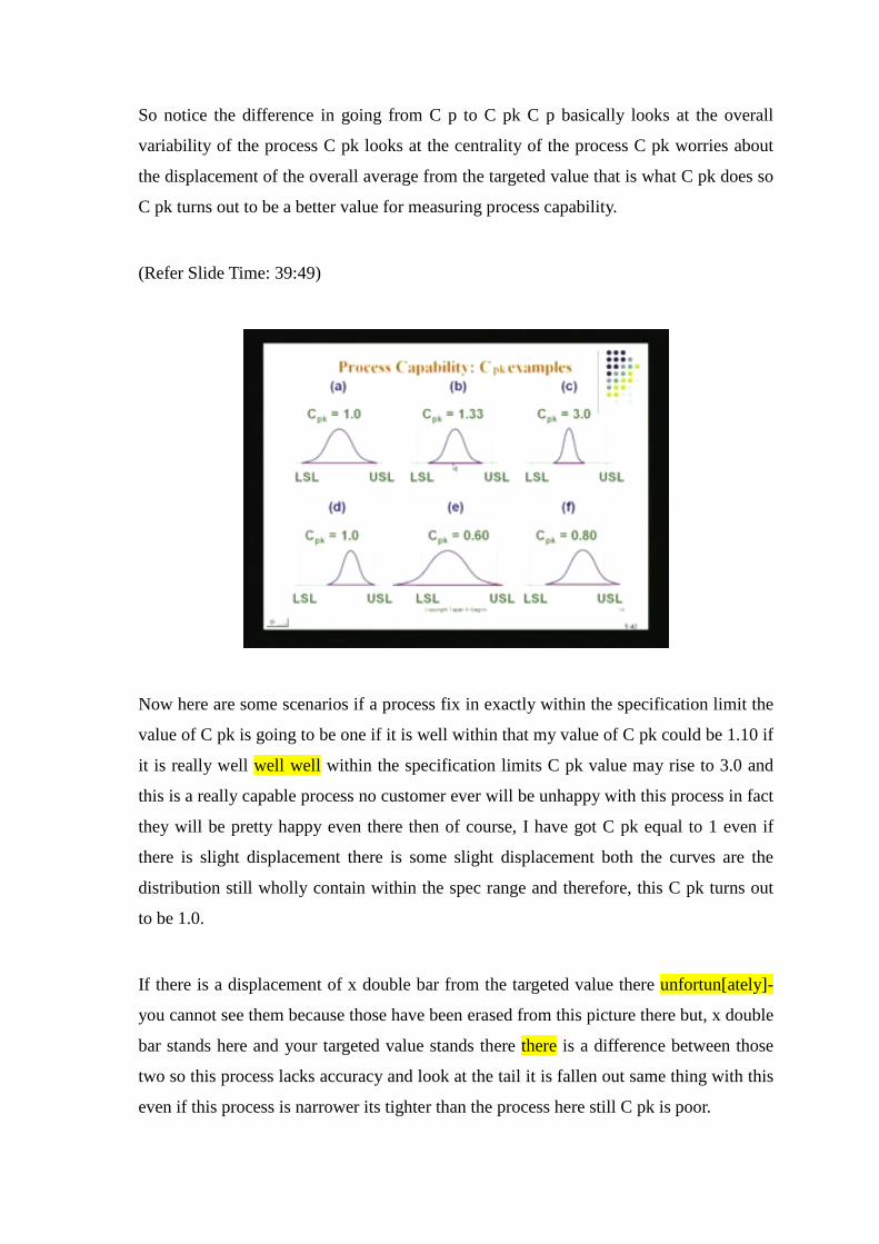
Now here are some scenarios if a process fix in exactly within the specification limit the

value of C pk is going to be one if it is well within that my value of C pk could be 1.10 if

it is really well well well within the specification limits C pk value may rise to 3.0 and

this is a really capable process no customer ever will be unhappy with this process in fact

they will be pretty happy even there then of course, I have got C pk equal to 1 even if

there is slight displacement there is some slight displacement both the curves are the

distribution still wholly contain within the spec range and therefore, this C pk turns out

to be 1.0.

If there is a displacement of x double bar from the targeted value there unfortun[ately]-

you cannot see them because those have been erased from this picture there but, x double

bar stands here and your targeted value stands there there is a difference between those

two so this process lacks accuracy and look at the tail it is fallen out same thing with this

even if this process is narrower its tighter than the process here still C pk is poor.

So it turns out to the best this situation to be in is to be well within the tolerance limits of

course, number one number two the average has to be pretty close to the target that is

there your process is very capable and this could be measured using this C pk process

capability index how do we improve it that couple of ways to do it.


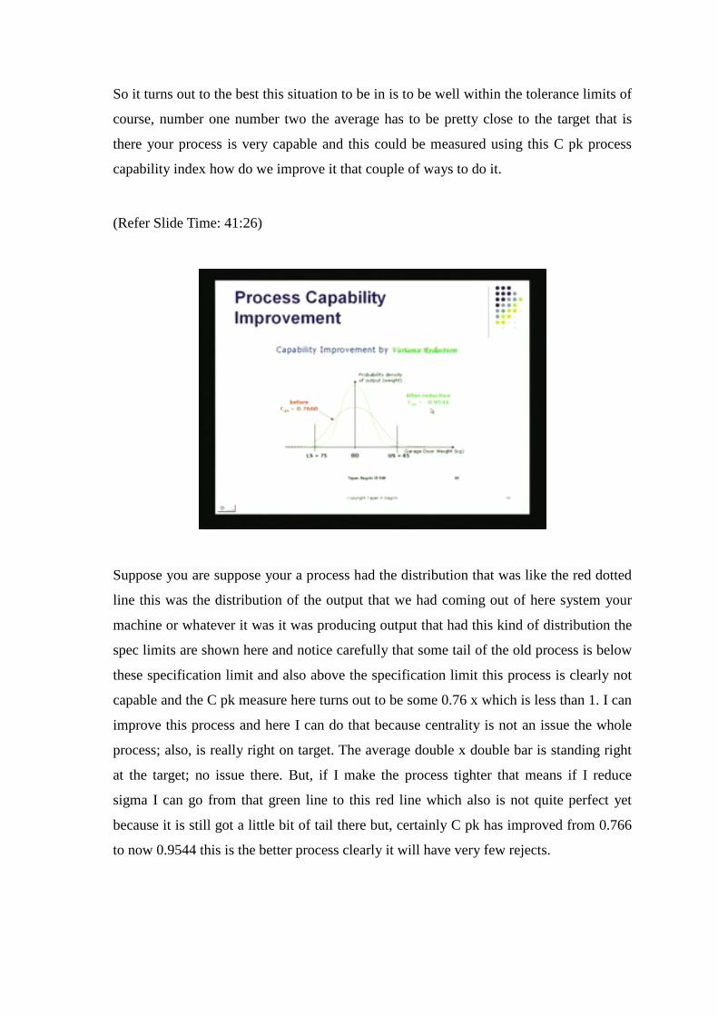
Suppose you are suppose your a process had the distribution that was like the red dotted

line this was the distribution of the output that we had coming out of here system your

machine or whatever it was it was producing output that had this kind of distribution the

spec limits are shown here and notice carefully that some tail of the old process is below

these specification limit and also above the specification limit this process is clearly not

capable and the C pk measure here turns out to be some 0.76 x which is less than 1. I can

improve this process and here I can do that because centrality is not an issue the whole

process; also, is really right on target. The average double x double bar is standing right

at the target; no issue there. But, if I make the process tighter that means if I reduce

sigma I can go from that green line to this red line which also is not quite perfect yet

because it is still got a little bit of tail there but, certainly C pk has improved from 0.766

to now 0.9544 this is the better process clearly it will have very few rejects.


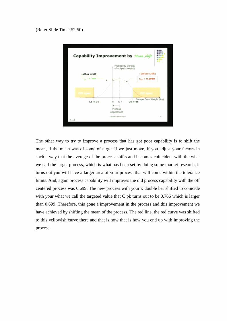
The other way to try to improve a process that has got poor capability is to shift the

mean, if the mean was of some of target if we just move, if you adjust your factors in

such a way that the average of the process shifts and becomes coincident with the what

we call the target process, which is what has been set by doing some market research, it

turns out you will have a larger area of your process that will come within the tolerance

limits. And, again process capability will improves the old process capability with the off

centered process was 0.699. The new process with your x double bar shifted to coincide

with your what we call the targeted value that C pk turns out to be 0.766 which is larger

than 0.699. Therefore, this gone a improvement in the process and this improvement we

have achieved by shifting the mean of the process. The red line, the red curve was shifted

to this yellowish curve there and that is how that is how you end up with improving the

process.


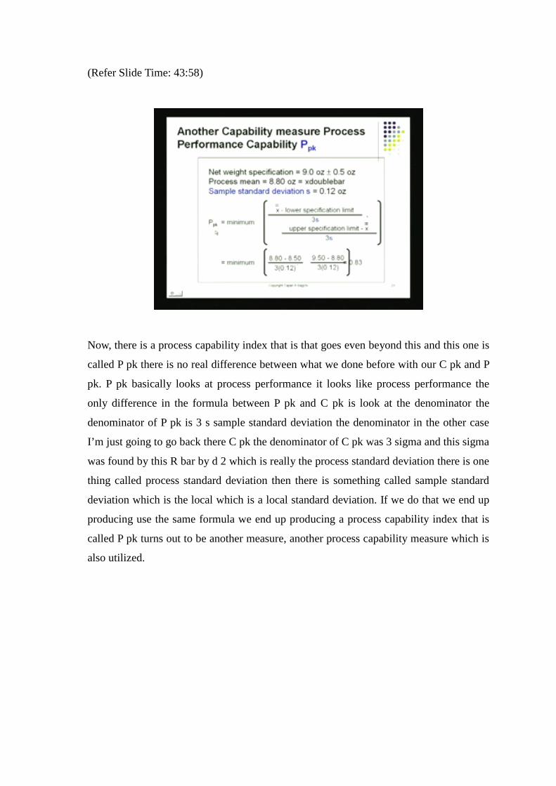
Now, there is a process capability index that is that goes even beyond this and this one is

called P pk there is no real difference between what we done before with our C pk and P

pk. P pk basically looks at process performance it looks like process performance the

only difference in the formula between P pk and C pk is look at the denominator the

denominator of P pk is 3 s sample standard deviation the denominator in the other case

I’m just going to go back there C pk the denominator of C pk was 3 sigma and this sigma

was found by this R bar by d 2 which is really the process standard deviation there is one

thing called process standard deviation then there is something called sample standard

deviation which is the local which is a local standard deviation. If we do that we end up

producing use the same formula we end up producing a process capability index that is

called P pk turns out to be another measure, another process capability measure which is

also utilized.


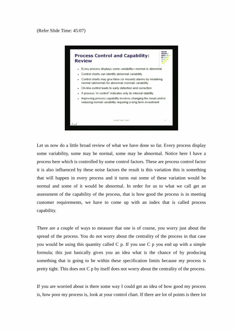
Let us now do a little broad review of what we have done so far. Every process display

some variability, some may be normal, some may be abnormal. Notice here I have a

process here which is controlled by some control factors. These are process control factor

it is also influenced by these noise factors the result is this variation this is something

that will happen in every process and it turns out some of these variation would be

normal and some of it would be abnormal. In order for us to what we call get an

assessment of the capability of the process, that is how good the process is in meeting

customer requirements, we have to come up with an index that is called process

capability.

There are a couple of ways to measure that one is of course, you worry just about the

spread of the process. You do not worry about the centrality of the process in that case

you would be using this quantity called C p. If you use C p you end up with a simple

formula; this just basically gives you an idea what is the chance of by producing

something that is going to be within these specification limits because my process is

pretty tight. This does not C p by itself does not worry about the centrality of the process.

If you are worried about is there some way I could get an idea of how good my process

is, how poor my process is, look at your control chart. If there are lot of points is there lot

of statistical points, these are the expired values of the R value. If they are beyond the

control limits clearly it is not very lightly that your process is capable this is something

you got to worry about so if you if you are starting out trying to control your process of

course, you could produce the histogram of the output and I could do that but, it will be

better idea to try to run a control chart and take a look at r there take a look at whether

there are many assignable causes that are also impact in the process control chart.

The process if the process is being influenced by lot of these what we call abnormal

causes or assignable causes spend some time to try to remove them once you remove

them what is left is just a chance causes; these are the random factors that will be there

no matter what unless you improve the technology of the process. if you improve the

technology you can of course, tighten of the process just like one great way to try to

improve your process.

So, control charts would be a pretty decent place to begin your study and take a look at

just in case this chart show some sort of normal variability it is possible that control

charts would give you false signals. It is very possible that the variation that you see is

normal but, remember alpha error; alpha error is the type of an error control committed

with a control chart which says I get a signal that means I see a point beyond what we

call control limit upper and lower control limits on a control chart. And, I go which

hunting I tried to sort of diagnose the process I go back to my process and I start taking a

look at all these different factors to try to see is there something wrong with A? Is there

something wrong with B? Is there something with C? This investigated little bit more to

try to sort out so it can be removed something there.

Suppose the process was not disturbed, you would have adjusted statistical variation that

lead to that condition. There you will end up with the process you will end up needless to

troubleshoot in the process. So, that can happen because the control chart you know there

is like a tiny chance 3 or 4 parts per 1000 when the chart itself may give you false signal

that is there and this is the type 1 error. If we do, now what we call in control? If we

remove assignable causes and what we are left with is basically essentially the process

under the influence of chance causes only which is the natural variation of the process it

is at that point. You can try to, you should to make an assessment of what we call process

capability. Process capability is the capability of the process to be able to just basically

produce any output. It will meet customer requirements it is wholly within the tolerance

that is tolerated by the customer if it is if there is a process like that you have nothing to

worry about it. I should of course, caution you that many times the range of the process

that means the difference between the maximum value of the output produced on

minimum value it may be pretty tight but, the overall process itself may be aspect and

that is because sometimes the average which is x w bar may not ( ) inside with the target

mu.

If x w bar are mu if they are different from each other this will cause this will cause some

part of the process to go beyond the control limits even in the process has descent

distribution as we saw in one of the earlier curve curves so what we have to do is we

have to do two things now the first thing is get an idea of process variability which you

could do just using C p plot some charts try to make sure that there are no assignable

causes present in process that disturb the process. This is something you have to do. The

third thing you have to do is compute C pk and C pk will tell you if there is a problem of

basically positioning the process which means is it being is it running right.

Now, the average quantity is average quality characteristic being produced there are

beyond what we call either below or above the target that is desired by the customer. If it

is off target that means, there is a problem with the process there to do some adjustment

to try to make sure the average returns to the target value. Then, I have got the best

process then of course, I am going to tighten of the process.

The methods for doing this, some of this can be done through experience a better way to

do this is to apply a design of experiments, use factors and those factors eventually will

end up tackling your process there and they will come up with those factors that really

cause either a shift in mean or a shift in sigma that can be done by doing by picking the

right response making the right measurements and conducting experiments in the frame

work of what we call a matrix. If you do those matrix experiments you are very lightly to

discover the main effect of the different factors that are there the process control factors

and also their interaction. Once that is there, once these variations have been located you

got not much to worry about. All you have to do is adjust the process, adjust those these

settings on those factors, the factors that turn out to be the culprits. You adjust them in

the right direction, the process will be stored. The average will come back x w bar will

come back to target and also sigma will reduce sigma, will reduce the overall variance of

the process will reduce this is something that we need to do.


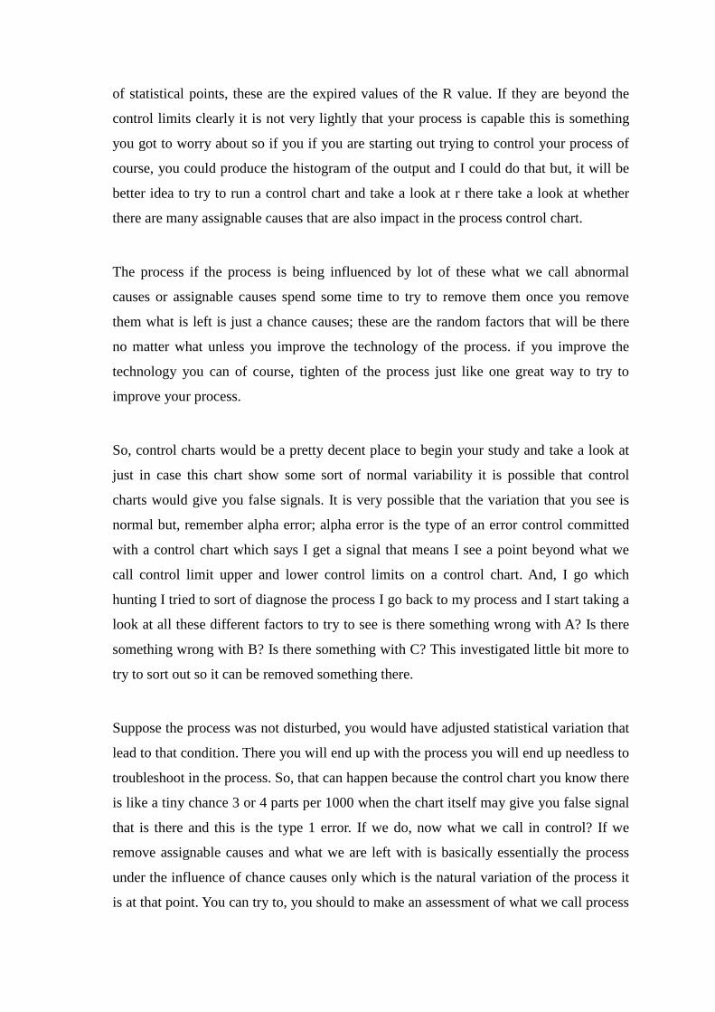
This is a very interesting area in fact designed very often aims at simplifying it, looks at

simpler parts, pure parts and so on and so forth. Always the idea is to try to come up with

the process which has got easy to operate which is easy to operate, easy to assemble,

easy to produce and any chance of making human error those also have been reduced

those have been minimized. You look at the causes of variation look at the causes of

variation; you monitor the process using a control chart you look at the output. If it turns

out that the you got a lot of assignable factors there then of course, you go back there do

investigation there.

If you are taking care of the assignable factors then, you look at the spread of the

process. You look at the spread of the process because that is now the natural variation of

the process if that goes either above or below what we call the tolerance you have to then

adjust, you have to then play with the sigma of the process and this again like I said it

that can be done. This is the overall variability of the process and one great way to tackle

that is to apply design of experiments.

So, we wrap up this session by saying if there is a process that is influenced by many

factors I can monitor using process control charts. And, then of course, I have got this

tool called C p or C pk measurement. These give you a pretty descent idea see the

process control charts themselves they do not talk about specification but, the moment

you bring in C p or C pk you talking specification and now you are talking about what is

of interest to the customer, to the final user. If you do this, your process will stay in

control. Also, it will consistently produce output that is well within the tolerance that is

tolerated by the customer; we will continue our series with the next lecture; thank you

very much.

Documents

Six Sigma Prof. Dr. T. P. Bagchi Department of …textofvideo.nptel.ac.in/110105039/lec24.pdfSo this in fact goes on and on and on it moves like a cycle you have control then improve