Embed Size (px)
Citation preview

Six DOF Motion Estimation for Teleoperated Flexible Endoscopes
Using Optical Flow: A Comparative Study
Charreau S. Bell, Gustavo A. Puerto, Gian-Luca Mariottini, and Pietro Valdastri
Abstract— Colorectal cancer is one of the leading causes ofcancer-related deaths worldwide, although it can be effectivelytreated if detected early. Teleoperated flexible endoscopes arean emerging technology to promote participation in thesepreventive screenings. Real-time pose estimation is thereforeessential to enable feedback to the robotic endoscope’s controlsystem. Vision-based endoscope localization approaches are apromising avenue, since they do not require extra sensors onboard the endoscopes. In this work, we compare several state-of-the-art algorithms for computing the image motion (opticalflow), which is then used with a supervised learning strategyto provide an accurate estimate of the 6 degree of freedomendoscope motion. The method is validated using a roboticallyactuated endoscope in a human colon simulator, and representsa preliminary effort towards testing with clinical video data.
I. INTRODUCTION
Colorectal cancer is the fourth leading cause of cancer
mortality in the world, with more than 63% of these deaths
occurring in developed nations [1], [2]. Unlike many other
types of cancer, colorectal cancer can almost always be
prevented by regular screenings for patients over 50 or with
a family history of colon cancer. By detection at an early
stage, the prognosis for survival is 90%, whereas if detected
too late, it decreases to 5% [3].
The traditional method for colorectal cancer screening is
through colonoscopy, a procedure in which a 1.5m flexible
endoscope is inserted into the colon for the detection and
removal of lesions and polyps. Colonoscopy is an outpatient
procedure, is performed under sedation, and only takes
about 30 minutes. Despite these favorable conditions and the
clear advantages of compliance with the recommendation for
cancer screening, nearly one-third of the population at risk
avoid the procedure [4].
In an effort to encourage patient participation and increase
the polyp detection rate, fully- and semi-automatic robotic
endoscopes are emerging in the field [3], [5]–[8]. This
approach focuses the doctor’s attention on polyp detection,
and reduces the physically demanding maneuvering of the
endoscope, which requires years of training for proficiency.
The compliancy of colon tissue and its variability among
patients presents a challenge for creating an accurate model
C.S. Bell and P. Valdastri are with the Department of MechanicalEngineering, Vanderbilt University, 506 Olin Hall, Nashville, TN 37235,USAEmail:[email protected]@vanderbilt.edu
G. Puerto and G.L. Mariottini are with the Department of ComputerScience and Engineering, University of Texas at Arlington, 416 Yates Street,Arlington, TX 76019, USA.Email:[email protected]@uta.edu
of the colon for open-loop control for robotic endoscopes. In-
stead, closed-loop control, which is effective for disturbance
rejection and error minimization, can decrease the difference
between the target actuation pose versus the actual reached
pose of the endoscopic camera head.
Real-time pose detection is therefore essential to enabling
feedback to the robotic endoscope’s control system. Mag-
netic tracking is a reliable method for localization; however,
this can possibly increase the endoscope size or occupy
the tool channel. Furthermore, the accuracy and reliability
of a magnetic tracker can be potentially compromised by
interfering magnetic fields from the permanent magnets
of emerging teleoperable platforms that are being pursued
commercially and by research labs worldwide [9]–[12].
Image processing provides a valid alternative avenue for
localization. One popular method in medicine is through
global localization by means of image registration; however,
because of the large deformations of the soft colon body
during a colonoscopy, global localization is ineffective in
practice. Optical flow techniques avoid this limitation, as they
provide information about the frame-to-frame changes to
compute the motion of the endoscope tip. Such a localization
scheme that neither increases the size of the endoscope nor
interferes with the robotic platform, but produces reliable and
accurate pose estimates, is a favorable method for providing
pose feedback for teleoperated flexible endoscopes.
A. Related Work
Usage of the endoscopic camera stream has mainly fo-
cused on locating gastrointestinal structural landmarks or le-
sions. These large-scale features include the lumen [13], [14]
and haustral folds [15]–[17]. The usage of machine learning
and artificial intelligence methods for navigation within the
colon has also been limited to detecting gastrointestinal
structural landmarks via pattern recognition classifiers [18],
and rule-based systems using fuzzy logic [15].
Motion estimation and navigation based on image motion
analysis for navigation have been successfully used for other
applications, including mobile robot and vehicle navigation.
Common techniques include optical flow, and modeling of
the camera [19], although scale cannot be recovered by these
methods alone. Within gastrointestinal endoscopy, navigation
has been achieved by adjusting the current heading towards
the lumen center in each control loop by employing the
spherical camera model [6]. Focus of expansion and optical
flow approaches have also been successfully employed on
virtual colonoscopy and other real endoscopic image sets [7],
[20], [21]. However, algorithm performance on computer-
2014 IEEE International Conference on Robotics & Automation (ICRA)
Hong Kong Convention and Exhibition Center
May 31 - June 7, 2014. Hong Kong, China
978-1-4799-3684-7/14/$31.00 ©2014 IEEE 5386
generated datasets can differ significantly from a colon
simulator or human colon [6], and none of these approaches
are able to provide quantitative information about the full 6
degree of freedom (DOF) change of pose of the endoscope
tip. Additionally, many of these methods assume that a focus-
of-expansion can be detected in the image, which might not
happen in the frequent case of rotational motions of the
endoscope.
B. Original Contribution and Organization
The original contribution of this paper is to compare
the effects of several state-of-the-art optical flow estimation
algorithms on their capability to best describe the movement
between images of the colon typically observed during a
colonoscopy. The efficacy of these optical flow measure-
ments resulting from each of these methods is measured by
the accuracy of a supervised learning localization strategy
that maps these image variations to 6 DOF changes in pose
of the endoscope.
Applying artificial neural networks (ANN) to derive the
change in pose of robotic endoscopes has been proposed
[22]. In this study, different sources of illumination (white
light and narrow band) and image partitioning (grid-based
and lumen-centered) were compared to investigate the com-
bination providing the strongest features to drive the ANN.
A standard Lucas-Kanade (LK) method was adopted to
compute the sparse optical flow. In this paper, we build upon
this previous work by providing an extensive comparison
of several of the most important optical flow computation
methods.
The paper is organized as follows: Sect. II presents an
overview of the optical flow methods adopted in our work,
together with a description of their major advantages and
disadvantages. Sect. III describes the supervised-learning
localization strategy, while Sect. IV presents both the experi-
mental setup and the results of the comparison between each
optical flow method. Finally, Sect. V highlights the major
conclusions and describes future work.
II. OVERVIEW OF OPTICAL FLOW COMPUTATION
In this section, we present an overall description of the
state-of-the-art algorithms we adopted for the computation
of the image motion (optical flow) across consecutive frames
of an endoscopic video. Since a comparison between all the
optical flow algorithms designed over the past decades is
unfeasible in this conference paper, we decided to focus on
a subset of representative methods. In particular, we selected
those methods that are most popular and with important
peculiar features, such as invariance to illumination or rapid
camera motion. The mathematical and implementation de-
tails for each method are outside the scope of this work and
can be obtained from the references provided below.
A. Lucas-Kanade (LK) based optical flow
We adopted the Lucas-Kanade method [23] for computing
the optical flow between two frames of an endoscopic video.
LK estimates the image motion of image templates across
(a) It−∆t (b) It
(c) LK (d) SURF
(e) SIFT (f) dHMA
Fig. 1. Representative Optical Flows: (a)-(b) Frames It−∆t and It; (c)Lucas-Kanade (LK); (d) Scale-invariant (SURF); (e) Scale-invariant (SIFT);(f) Dense Hierarchical Multi-Affine (dHMA).
two consecutive frames, It−∆t and It (cf., Fig. 1(a)-1(b)),
of an endoscopic video. As commonly done in the literature,
we centered each template at a Shi-Tomasi feature [24]. We
adopted a pyramidal multi-resolution implementation of the
LK method [25] that provides a more reliable estimation
when compared to traditional LK implementations.
Figure 1(c) illustrates an example of the optical flow
vectors (blue) computed by LK. Each flow vector is centered
at a Shi-Tomasi corner. Because of the presence of many
textureless areas and image blurs, the resulting LK-based
optical flow is usually very sparse, since only few Shi-
Tomasi features are detected in these areas. There are two
key assumptions in the LK method: the first one assumes
brightness constancy over time of the two frames, and
the second assumes small motion of each template across
consecutive frames, allowing filtering of noisy flow vectors
with very large magnitude (outliers).
B. Scale-Invariant optical flow
In order to robustly estimate the optical flow in the case
of large endoscope motion and changes in illumination, we
adopted two scale-invariant features: SIFT (Scale-Invariant
Feature Transform) [26] and SURF (Speeded-Up Robust
Features). These features are extracted and matched in two
consecutive frames to find the optical flow. We decided to
focus on these two algorithms because of their proved high-
5387

repeatability (SIFT), speed (SURF), and because of their
good matching and accuracy rates (SURF and SIFT) in many
challenging conditions.
The main advantage of these scale-invariant features, when
compared to other feature extraction and matching methods,
is that a descriptor is computed from the image portion
around each keypoint (i.e., an image patch, edge, or corner).
The importance of descriptors is that they contain a statistical
representation of the image gradients around each local
image portion. As such, the descriptor is what makes SIFT
and SURF invariant to changes in scale and rotation, and
robust to changes in illumination and viewpoint [27].
Figure 1(e) illustrates the optical flow obtained with SIFT
descriptors between two sequential frames. SIFT (as well
as SURF) can extract optical flow vectors in (small) areas
with uniform texture. However, it is possible to still see the
presence of a few wrong flow vectors (outliers) caused by
the erroneously-matched descriptors.
In our implementation, we tested several keypoint detec-
tors, being FAST keypoint [28] the one that offered better
results in this scenario.
C. Dense Hierarchical Multi-Affine (dHMA) optical flow
We adopted two dense optical-flow methods that were
proved to have a reduced outlier ratio when compared to
SIFT and SURF, especially when applied to endoscopic
images. In particular, we adopted HMA [29], [30] and
dHMA [31]; the latter can (densely) estimate the optical flow
vectors over the entire image, and thus cover large textureless
areas. Differently from other dense optical-flow methods that
take tens of seconds, HMA and dHMA almost runs in real
time (∼ 80ms for HMA, and ∼ 1sec. for dHMA) in our
MATLAB implementation.
Both HMA and dHMA match sparse feature descriptors1
while eliminating the majority of outliers by means of a
robust hierarchical estimation of multi-affine transforma-
tions. dHMA has an additional step in which the resulting
inliers are given in input to a Gaussian-Process regression
stage [32] that estimates a dense mapping function. This
function (or the multi-affine maps from HMA) model the
non-rigid motion of a given set of image points over the
entire image (ideally, for every pixel).
Figure 1(f) shows the optical flow vectors calculated by
dHMA for a pre-defined grid of image points. Since these
points do not necessarily coincide with image features (e.g.,
corners), the resulting optical flow can be computed over
large textureless areas, and with few outliers. Compared to
the aforementioned optical-flow estimation methods, HMA
and dHMA have great accuracy, can eliminate outliers, are
automatic, and require very minimal number of tuning pa-
rameters from the user. Our previous results [31] experiments
showed that dHMA can achieve a slight better accuracy than
HMA.
1In our implementation, HMA and dHMA uses SIFT descriptors.
(a) (b)
Fig. 2. Spatial partitioning rules for creating the optical flow descriptorsfrom an optical flow field. (a) Grid-based partitioning. (b) Lumen-centeredpartitioning.
III. FLOW DESCRIPTORS AND LOCALIZATION STRATEGY
The proposed method estimates the 6 DOF change in pose
of the endoscope camera tip using only optical flow data
computed as described in Sect. II. The scene viewed by the
camera is assumed to be static between two frames; this is
a valid assumption since large-scale motion in the colon is
limited to haustral contractions (i.e., motion which moves
the contents of the colon forward). These movements occur
relatively rarely (once every 30 minutes) [33]. Regardless,
specialized control loops using histogram analysis and other
heuristics can be implemented to mitigate the effects of
sporadic deviations from these assumption.
The optical flow vector field extracted at each time instant
over the entire image is combined into a single representative
vector, referred to as the optical flow descriptor. We examine
two distinct ways of combining the entire flow field at each
frame into a single descriptor: a grid-based or a lumen-
centered partition. These optical flow descriptors, together
with a known metric change in pose of the endoscope, com-
pose the training set for a supervised learning method, specif-
ically, an artificial neural network (ANN). Once trained, the
ANN provides an associative model of the system for real-
time pose feedback; given only the relative motion in the
image, the ANN is able to estimate the change in pose of
the endoscope tip.
A. Feature Descriptor Generation
Figure 3 outlines the process for computing the change in
pose from the endoscopic camera sequence. At times t−∆t
and t, images are captured from the camera.2 These two
images are then used to compute the optical flow according
to the methods presented in Section II.
The entire optical flow is then used to create a single
optical flow descriptor. Two different image partitioning
methods were adopted and compared: a standard grid-based
partitioning (cf., Fig. 2(a)), and lumen-centered partitioning
(cf., Fig. 2(b)).
The grid-based partitioning method divides the image into
a 5x5 grid (i.e., 25 sections) of equal rectangular areas.
The ng optical flow vectors inside each region g of the
2A mask was applied in order to only include the effective pixels in theimage in the algorithm, and disregard any text present in the image.
5388
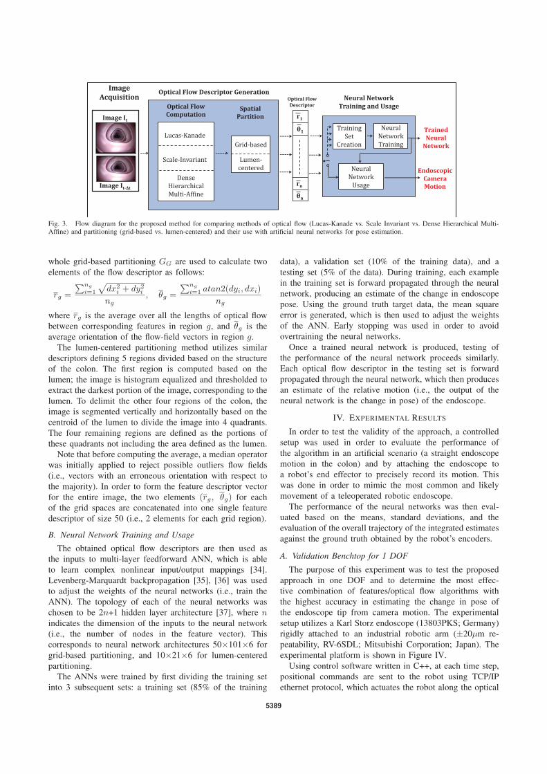
Image It
Image It- t
Image
Acquisition Optical Flow Descriptor Generation
Optical Flow
Computation Spatial
Partition
Grid-based
Lumen-
centered
Neural Network
Training and Usage Optical Flow
Descriptor
Training
Set
Creation
Neural
Network
Training
Neural
Network
Usage
Endoscopic
Camera
Motion
Trained
Neural
Network
Lucas-Kanade
Scale-Invariant
Dense
Hierarchical
Multi-Affine
r1
1
rn
n
Fig. 3. Flow diagram for the proposed method for comparing methods of optical flow (Lucas-Kanade vs. Scale Invariant vs. Dense Hierarchical Multi-Affine) and partitioning (grid-based vs. lumen-centered) and their use with artificial neural networks for pose estimation.
whole grid-based partitioning GG are used to calculate two
elements of the flow descriptor as follows:
rg =
∑ng
i=1
√
dx2i + dy2i
ng
, θg =
∑ng
i=1atan2(dyi, dxi)
ng
where rg is the average over all the lengths of optical flow
between corresponding features in region g, and θg is the
average orientation of the flow-field vectors in region g.
The lumen-centered partitioning method utilizes similar
descriptors defining 5 regions divided based on the structure
of the colon. The first region is computed based on the
lumen; the image is histogram equalized and thresholded to
extract the darkest portion of the image, corresponding to the
lumen. To delimit the other four regions of the colon, the
image is segmented vertically and horizontally based on the
centroid of the lumen to divide the image into 4 quadrants.
The four remaining regions are defined as the portions of
these quadrants not including the area defined as the lumen.
Note that before computing the average, a median operator
was initially applied to reject possible outliers flow fields
(i.e., vectors with an erroneous orientation with respect to
the majority). In order to form the feature descriptor vector
for the entire image, the two elements (rg, θg) for each
of the grid spaces are concatenated into one single feature
descriptor of size 50 (i.e., 2 elements for each grid region).
B. Neural Network Training and Usage
The obtained optical flow descriptors are then used as
the inputs to multi-layer feedforward ANN, which is able
to learn complex nonlinear input/output mappings [34].
Levenberg-Marquardt backpropagation [35], [36] was used
to adjust the weights of the neural networks (i.e., train the
ANN). The topology of each of the neural networks was
chosen to be 2n+1 hidden layer architecture [37], where n
indicates the dimension of the inputs to the neural network
(i.e., the number of nodes in the feature vector). This
corresponds to neural network architectures 50×101×6 for
grid-based partitioning, and 10×21×6 for lumen-centered
partitioning.
The ANNs were trained by first dividing the training set
into 3 subsequent sets: a training set (85% of the training
data), a validation set (10% of the training data), and a
testing set (5% of the data). During training, each example
in the training set is forward propagated through the neural
network, producing an estimate of the change in endoscope
pose. Using the ground truth target data, the mean square
error is generated, which is then used to adjust the weights
of the ANN. Early stopping was used in order to avoid
overtraining the neural networks.
Once a trained neural network is produced, testing of
the performance of the neural network proceeds similarly.
Each optical flow descriptor in the testing set is forward
propagated through the neural network, which then produces
an estimate of the relative motion (i.e., the output of the
neural network is the change in pose) of the endoscope.
IV. EXPERIMENTAL RESULTS
In order to test the validity of the approach, a controlled
setup was used in order to evaluate the performance of
the algorithm in an artificial scenario (a straight endoscope
motion in the colon) and by attaching the endoscope to
a robot’s end effector to precisely record its motion. This
was done in order to mimic the most common and likely
movement of a teleoperated robotic endoscope.
The performance of the neural networks was then eval-
uated based on the means, standard deviations, and the
evaluation of the overall trajectory of the integrated estimates
against the ground truth obtained by the robot’s encoders.
A. Validation Benchtop for 1 DOF
The purpose of this experiment was to test the proposed
approach in one DOF and to determine the most effec-
tive combination of features/optical flow algorithms with
the highest accuracy in estimating the change in pose of
the endoscope tip from camera motion. The experimental
setup utilizes a Karl Storz endoscope (13803PKS; Germany)
rigidly attached to an industrial robotic arm (±20µm re-
peatability, RV-6SDL; Mitsubishi Corporation; Japan). The
experimental platform is shown in Figure IV.
Using control software written in C++, at each time step,
positional commands are sent to the robot using TCP/IP
ethernet protocol, which actuates the robot along the optical
5389

Endoscopic
Column
Endoscope
Robotic Arm
Image Acquisition Endoscope
Tip
Colon
Simulator
Fig. 4. Experimental setup replication movements of a teleoperatedendoscope in a human colon simulator.
axis of the camera (the optical axis of the camera is aligned
with the x-axis of the robot). The endoscope moves along
a trajectory in the plastic human colon simulator (shown in
Figure IV) in increments of ∼ ±0.3mm from 0.3mm to 4mm
for 20 iterations each. This resulted in a data set of size
260, corresponding to 549mm of total movement. After a
one second time delay to avoid oscillation in the image due
to the actuation, the resultant frame is captured through a
frame grabber (EasyCAP; USB EasyCap Co., China) via S-
Video from the Karl Storz endoscopic column, alongside the
corresponding position of the robot. This is repeated until
the entire trajectory was completed.
Thanks to the rigid connection to the robot, the instan-
taneous motion can be easily deduced from the robot’s
encoders with high accuracy. This large dataset is then
subsampled into two mutually exclusive groups for the
training and testing data, using two-thirds of the data for
training, and one-third of the data for testing. The dataset
only includes straight sections of the colon. Since the weights
of ANNs are randomly generated, and are not guaranteed to
converge to a global minimum, 100 ANNs were generated
for each optical flow/partitioning method. Using the means
and standard deviations as a basis for evaluation, the best
ANNs were chosen to perform the estimations.
B. Experimental Results and Discussion
Figure 5 shows the pose estimation capabilities for each
of the optical flow methods using grid-based partitioning
and lumen-centered partitioning for 1 DOF robotic actuation
along a straight section of the colon. Figure 5(a) shows the
mean and the standard deviation of the incremental pose
error (i.e., between the output of the ANNs and the ground-
truth endoscope motion) for the grid-based partition. The
two dense optical flow methods performed similarly, with
an average absolute mean of 1.3mm±1.9mm error over the
moving direction (X axis), and outperformed the ANNs
resulting from the sparse optical flow methods. The absolute
mean errors using these methods spanned to 14.6mm using
FAST with SURF descriptors. Note in Figs. 5(a) and 6(a),
that the translation errors along the Y and Z axis are zero,
suggesting the ANNs capability to correctly identify the
moving direction. Moreover, our orientation errors were zero
Methods
X Y Z
Err
or
(in
mm
)
25
20
15
10
5
0
-5
(a)
Trajectory Step
Po
sitio
n (
in m
m)
0
10
20
30
40
50
60
-10
0 20 40 60 80
(b)
Fig. 5. Experimental results with grid-based partitioning. (a) Mean andstandard deviation of error. (b) Trajectory of endoscope as compared withground truth of robot encoders.
for both grid and lumen based ANNs, for this reason we
decided to do not include the orientation errors in Figs. 5-6,
as well as to limit our analysis to only the X axis.
For each method using the grid-based partition, the in-
tegration of the estimated incremental positions along the
X axis are shown in Fig. 5(b) to form the entire estimated
trajectory along the forward direction of the endoscope
during the trial. The dense optical flow techniques are best
able to produce nearly the same trajectory with a final
difference of 3.61mm over 174mm. FAST-SURF performed
the worst, with a deviation of 19.51mm from the intended
trajectory.
As for the performance of the optical flow methods using
the lumen-centered partition, FAST-SIFT, FAST-SURF, and
dHMA all perform similarly, with approximately 4-5mm
of mean absolute error over the entire test set. However,
unlike the grid-based partitioning, the LK method is able to
achieve the lowest absolute mean error (0.31mm), although
5390

Methods
X Y Z
Err
or
(in
mm
)
10
8
6
4
2
0
-2
-4
-6
-8
(a)
Po
sitio
n (
in m
m)
-10
0
10
20
30
40
0 20 40 60 80
Trajectory Step
(b)
Fig. 6. Experimental results with lumen-centered partitioning. (a) Meanand standard deviation of error. (b) Trajectory of endoscope as comparedwith ground truth of robot encoders.
it also possesses the highest standard deviation (±4.6mm).
On the other hand, HMA results in a slightly higher mean
error (1.45mm), but the standard deviation is much smaller
(±2.55mm).
Figure 6(b) demonstrates performance of these algorithms
over time when the changes in position are integrated to form
an entire trajectory. As shown, the mean of each algorithm
appears to correspond to an offset from the ground truth
data. For example, HMA, with a small mean and standard
deviation, is able to closely follow the trajectory until time
step 63. FAST-SIFT, FAST-SURF and dHMA exhibit larger
offsets during the trajectory, more evident during changes of
direction (peaks). Noteworthy is the performance of the LK
optical flow, whose sparse nature causes large standard devi-
ation causes unpredictable behavior in the motion estimation,
thus resulting in an unpredictable localization estimate.
Overall, the grid-based partition produces two of the
neural networks with the lowest error and smallest standard
deviation over both partitions; however lumen-centering par-
titioning appears to standardize the scene, which results in
lower error over all of the optical flow methods.
It is important to note that these results are dependent
on the training of the neural networks. Although 100 trials
were used in order to select the best neural network for each
optical flow/partitioning method, a more exhaustive number
of trials or averaging the outputs of all these neural networks
may represent a more reliable solution for comparing these
methods.
V. CONCLUSIONS AND FUTURE WORK
Colorectal cancer affects the lives of millions of people
worldwide; although almost always preventable, patients
avoid recommended colorectal cancer screening due to fear
of discomfort, and the perceived indignity of the procedure.
Teleoperable flexible endoscopes are emerging as a novel
method to abate these hindrances, but require closed-loop
control due to the complexities of the environment of the
colon. Pose detection using only the endoscopic camera
stream represents a favorable solution to this problem, since
it uses only components native to the endoscope, and can be
implemented across all teleoperable endoscopic platforms.
The proposed approach estimates the change in pose of
the endoscope by extracting the optical flow, the motion
between two sequential images. Five methods of calculating
the optical flow were compared: LK, FAST-SIFT, FAST-
SURF optical flow, HMA, and dHMA based on their ubiquity
in usage. Additionally, two partitioning methods - grid-based
and lumen-centered - were then compared to create single
optical flow descriptors for the optical flow in the entire
image. To produce a metric measurement of the change in
pose, an ANN was trained based on these inputs and the
known pose change of the endoscope.
This algorithm was then tested using an endoscope rigidly
attached to a robotic arm to mimic the expected movements
of a teleoperable flexible endoscope. The experiment was
performed on a human colon simulator in order to resemble
the endoscopic environment. Using the grid-based partition-
ing method, the dense optical flow algorithms were the most
accurate (1.3mm±1.9mm error; final difference in trajectory
3.61mm over 174mm).
Regarding the lumen-centered partitioning, the LK optical
flow resulted in the lowest mean error; however, the im-
precision of the algorithm caused large fluctuations in the
overall integrated trajectory. HMA provides the best perfor-
mance with lumen-centered partitioning (1.45mm±2.55mm);
it has the smallest standard deviation, and is able to closely
recreate the trajectory as given by ground truth. Between the
grid-based partitioning and the lumen-centered partitioning,
the grid-based partition produces the two best performing
neural networks as measured by their means and standard
deviations; however, the lumen-centered approach appears to
standardize the image, resulting in an overall lower average
error among all the techniques.
Future work includes investigating other robust, stable
features for detecting optical flow in the colon, investigat-
5391

ing other descriptor for representing the optical flow, and
finding the optimal method for mapping the optical flow
to the change in pose of the endoscope. Furthermore, more
extensive analysis needs to be done to quantify the sensitivity
of the ANNs to the size of the training set, as well as the
robustness to optical flow ambiguities caused by different
motions with similar optical flow. Additionally, in-vivo trials
will be performed in order to analyze the performance of
the algorithm on human colon tissue. From this, the impact
of haustal contractions and small movements of the colon
can be assessed. The performance of our algorithm indicates
that pose detection via supervised learning of optical flow is
a feasible feedback mechanism for implementing closed-loop
control of teleoperated flexible endoscopes.
REFERENCES
[1] F. Haggar and R. Boushey, “Colorectal cancer epidemiology: Inci-dence, mortality, survival, and risk factors,” Clinics in Colon and
Rectal Surgery, vol. 22, no. 4, pp. 191–197, 2009.
[2] Fact sheet # 297: Cancer. World Health Organization(WHO). Last accessed: 1 February 2012. [Online]. Available:www.who.int/mediacentre/factsheets/fs297/en .
[3] P. Valdastri, M. Simi, and R. J. Webster III, “Advanced technologiesfor gastrointestinal endoscopy,” Annual Review of Biomedical Engi-
neering, vol. 14, pp. 397–429, 2012.
[4] Vital Signs Cancer screening, colorectal cancer. Centers for DiseaseControl and Prevention. Last accessed: 1 February 2012. [Online].Available: www.cdc.gov/vitalsigns/CancerScreening/indexCC.html .
[5] K. L. Obstein and P. Valdastri, “Advanced endoscopic technologies forcolorectal cancer screening.” World J Gastroenterol, vol. 19, no. 4, pp.431–9, 2013.
[6] R. Reilink, S. Stramigioli, and S. Misra, “Three-dimensional posereconstruction of flexible instruments from endoscopic images,” inProceedings of the 2011 IEEE/RSJ International Conference on In-
telligent Robots and Systems, 2011, pp. 2076–2082.
[7] N. van der Stap, R. Reilink, S. Misra, I. Broeders, and R. van derHeijden, “The use of the focus of expansion for automated steering offlexible endoscopes,” in 4th IEEE RAS EMBS International Conference
on Biomedical Robotics and Biomechatronics (BioRob), 2012, pp. 13–18.
[8] J. Ruiter, E. Rozeboom, M. van der Voort, M. Bonnema, andI. Broeders, “Design and evaluation of robotic steering of a flexibleendoscope,” in 4th IEEE RAS EMBS International Conference on
Biomedical Robotics and Biomechatronics (BioRob), 2012, pp. 761–767.
[9] J. Rey, H. Ogata, N. Hosoe, K. Ohtsuka, N. Ogata, K. Ikeda, H. Aihara,I. Pangtay, T. Hibi, S. Kudo, and H. Tajiri, “Blinded nonrandomizedcomparative study of gastric examination with a magnetically guidedcapsule endoscope and standard videoendoscope,” Gastrointestinal
Endoscopy, vol. 75, no. 2, pp. 373–381, 2012.
[10] J. Keller, C. Fibbe, F. Volke, J. Gerber, A. C. Mosse, M. Reimann-Zawadzki, E. Rabinovitz, P. Layer, D. Schmitt, V. Andresen,U. Rosien, and P. Swain, “Inspection of the human stomach usingremote-controlled capsule endoscopy:a feasibility study in healthyvolunteers (with videos),” Gastrointestinal Endoscopy, vol. 73, no. 1,pp. 22–28, 2011.
[11] P. Valdastri, G. Ciuti, A. Verbeni, A. Menciassi, P. Dario, A. Arezzo,and M. Morino, “Magnetic air capsule robotic system: proof of conceptof a novel approach for painless colonoscopy,” Surgical Endoscopy,vol. 26, no. 5, pp. 1238–46, 2011.
[12] X. Wang, M. Meng, and X. Chen, “A locomotion mechanism withexternal magnetic guidance for active capsule endoscope,” in 32nd
Annual International Conference of the IEEE Engineering in Medicine
and Biology Society, 2010, pp. 4375–4378.
[13] G. Khan and D. Gillies, “Vision based navigation system for anendoscope,” Image and Vision Computing, vol. 14, no. 10, pp. 763– 772, 1996.
[14] X. Zabulis, A. Argyros, and D. Tsakiris, “Lumen detection for cap-sule endoscopy,” in Proceedings of the 2008 IEEE/RSJ International
Conference on Intelligent Robots and Systems, 2008, pp. 3921–3926.
[15] S. Krishnan, C. Tan, and C. Chan, “Closed-boundary extraction oflarge intestinal lumen,” in Proceedings of the 16th Annual Interna-
tional Conference of the IEEE Engineering in Medicine and Biology
Society, vol. 1, 1994, pp. 610–611.[16] H. Tian, T. Srikanthan, and K. Asari, “Automatic segmentation algo-
rithms for the extraction of lumen region and boundary from endo-scopic images,” Medical and Biological Engineering and Computing,vol. 39, no. 1, pp. 8–14, 2001.
[17] S. Xia, S. Krishnan, M. Tjoa, and P. Goh, “A novel methodologyfor extraction colon’s lumen from colonoscopic images,” Journal of
Systemics, Cybernetics and Informatics, vol. 1, no. 2, pp. 7–12, 2003.[18] J. Bulat, K. Duda, M. Duplaga, R. Fraczek, A. Skalski, M. Socha,
P. Turcza, and T. Zielinski, “Data processing tasks in wireless GIendoscopy: Image-based capsule localization & navigation and videocompression,” in Proceedings of the 29th Annual International Con-
ference of the IEEE Engineering in Medicine and Biology Society,2007, pp. 2815–2818.
[19] R. Hartley and A. Zisserman, Multiple View Geometry in Computer
Vision, 2nd ed. New York, NY, USA: Cambridge University Press,2003.
[20] J. Liu, T. Yoo, K. Sabramanian, and R. V. Uitert, “A stable optic-flow based method for tracking colonoscopy images,” in Proceedings
of the 2008 IEEE Computer Society Conference on Computer Vision
and Pattern Recognition Workshops, June 2008, pp. 1–8.[21] J. Liu, K. Subramanian, and T. Yoo, “Towards designing an optical-
flow based colonoscopy tracking algorithm: a comparative study,” inProc. SPIE, 2013, pp. 867 103–867 107.
[22] C. Bell, P. Valdastri, and K. Obstein, “Image partitioning and il-lumination in image-based pose detection for teleoperated flexibleendoscopes,” Artificial Intelligence in Medicine, vol. 59, no. 3, pp.185–196, 2013.
[23] B. D. Lucas and T. Kanade, “An iterative image registration techniquewith an application to stereo vision,” in Proceedings of the 7th
International Joint Conference on Artificial Intelligence (IJCAI), 1981,pp. 674–679.
[24] J. Shi and C. Tomasi, “Good features to track,” in Proceedings of the
IEEE Conference on Computer Vision and Pattern Recognition, 1994,pp. 593–600.
[25] G. Bradski, “The OpenCV Library,” Dr. Dobb’s Journal of Software
Tools, 2000.[26] D. G. Lowe, “Distinctive image features from scale-invariant key-
points,” Int. J. Comput. Vision, vol. 60, no. 2, pp. 91–110, November2004.
[27] K. Mikolajczyk and C. Schmid, “A performance evaluation of localdescriptors,” IEEE Transactions on Pattern Analysis and Machine
Intelligence, vol. 27, no. 10, pp. 1615–1630, 2005.[28] E. Rosten and T. Drummond, “Machine learning for high-speed
corner detection,” in Proceedings of the 9th European conference on
Computer Vision, 2006, pp. 430–443.[29] G. Puerto-Souza and G. Mariottini, “A fast and accurate feature-
matching algorithm for minimally-invasive endoscopic images,” IEEE
Transactions on Medical Imaging, vol. 32, no. 7, pp. 1201–1214, July2013.
[30] ——, “HMA feature-matching toolbox,” [Web:]http://ranger.uta.edu/%7egianluca/feature%5fmatching .
[31] ——, “Wide-baseline dense feature matching for endoscopic images,”in 6th Pacific Rim Symposium in Advances in Image and Video
Technology, PSIVT 2013, November 2013, in press.[32] C. Rasmussen and C. Williams, Gaussian processes for machine
learning. MIT press Cambridge, MA, 2006, vol. 1.[33] L. Sherwood, Human Physiology: From Cells to Systems, 6th ed.
Thomson Brooks/Cole, Pacific Grove, CA, USA, 2007.[34] G. Cybenko, “Approximation by superpositions of a sigmoidal func-
tion,” Mathematics of Control, Signals, and Systems (MCSS), vol. 2,no. 4, pp. 303–314, 1989.
[35] K. Levenberg, “A method for the solution of certain nonlinear prob-lems in least squares,” Quarterly of Applied Mathematics, vol. 2, pp.164–168, 1944.
[36] D. Marquardt, “An algorithm for least-squares estimation of nonlinearparameters,” SIAM Journal on Applied Mathematics, vol. 11, no. 2,pp. 431–441, 1963.
[37] R. Hecht-Nielsen, “Kolmogorov’s mapping neural network existencetheorem,” in Proceedings of the IEEE First Annual International
Conference on Neural Networks, S. Grossberg, Ed., vol. 3, 1987, pp.11–14.
5392