A Faster Algorithm for Computing Straight Skeletons

Siu-Wing Cheng Liam Mencel Antoine Vigneron

July 16, 2014

Abstract

We present a new algorithm for computing the straight skeleton of a polygon. For a polygon with nvertices, among which r are reflex vertices, we give a deterministic algorithm that reduces the straightskeleton computation to a motorcycle graph computation in O(n(logn) log r) time. It improves onthe previously best known algorithm for this reduction, which is randomized, and runs in expectedO(n

√h + 1 log2 n) time for a polygon with h holes. Using known motorcycle graph algorithms, our

result yields improved time bounds for computing straight skeletons. In particular, we can computethe straight skeleton of a non-degenerate polygon in O(n(logn) log r + r4/3+ε) time for any ε > 0. Ondegenerate input, our time bound increases to O(n(logn) log r + r17/11+ε).

1 Introduction

The straight skeleton of a polygon is defined as the trace of the vertices when the polygon shrinks, each edgemoving at the same speed inwards in a perpendicular direction to its orientation. (See Figure 1.) It differsfrom the medial axis [8] in that it is a straight line graph embedded in the original polygon, while the medialaxis may have parabolic edges. The notion was introduced by Aichholzer et al. [2] in 1995, who gave theearliest algorithm for computing the straight skeleton. However, the concept has been recognized as earlyas 1877 by von Peschka [24], in his interpretation as projection of roof surfaces.

The straight skeleton has numerous applications in computer graphics. It allows one to compute offsetpolygons [16], which is a standard operation in CAD. Other applications include architectural modelling [22],biomedical image processing [9], city model reconstruction [11], computational origami [12, 13, 14] andpolyhedral surface reconstruction [3, 10, 17]. Improving the efficiency of straight skeleton algorithms increasesthe speed of related tools in geometric computing.

The first algorithm by Aichholzer et al. [2] runs in O(n2 log n) time, and simulates the shrinking processdiscretely. Eppstein and Erickson [16] developed the first sub-quadratic algorithm, which runs in O(n17/11+ε)time. In their work, they proposed motorcycle graphs as a means of encapsulating the main difficulty in com-puting straight skeletons. Cheng and Vigneron [7] expanded on this notion by reducing the straight skeletonproblem in non-degenerate cases to a motorcycle graph computation and a lower envelope computation.This reduction was later extended to degenerate cases by Held and Huber [19]. Cheng and Vigneron gavean algorithm for the lower envelope computation on a non-degenerate polygon with h holes, which runs in

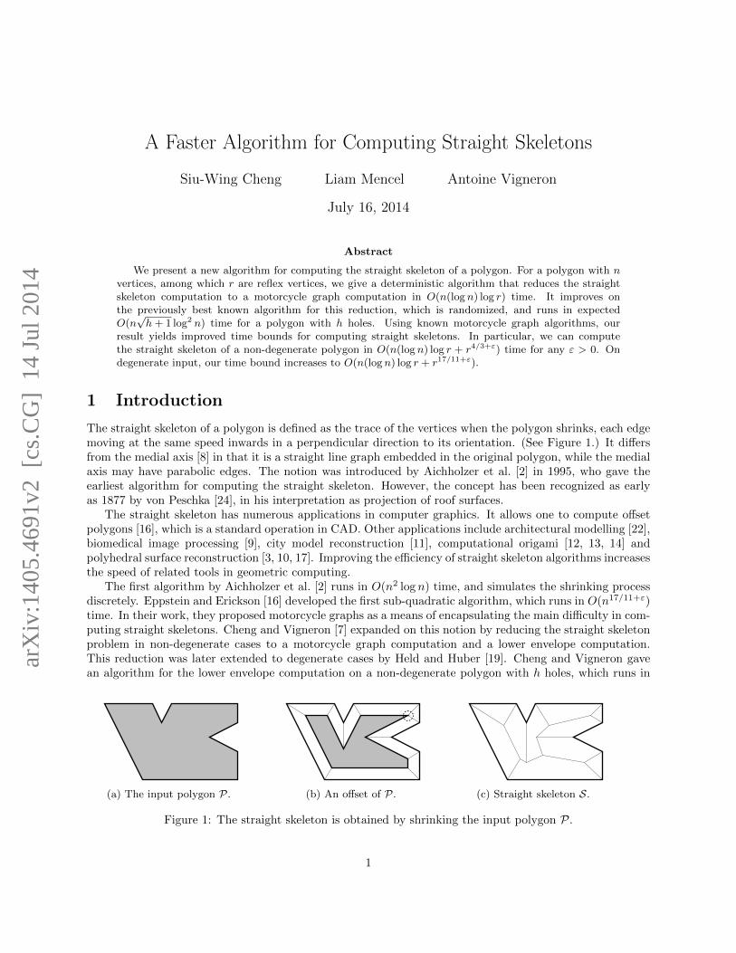
(a) The input polygon P. (b) An offset of P. (c) Straight skeleton S.

Figure 1: The straight skeleton is obtained by shrinking the input polygon P.

1

arX

iv:1

405.

4691

v2 [

cs.C

G]

14

Jul 2

014

Previously best known This paper

Arbitrary polygon O(n8/11+εr9/11+ε) [16] O(n(log n) log r + r17/11+ε)

Non-degenerate polygon O∗(n√r log2 n) [7] O(n(log n) log r + r4/3+ε)

Simple pol., arbitrary O∗(n log2 n+ r17/11+ε) [7, 16] O(n(log n) log r + r17/11+ε)

Simple pol., O(log n) bits O∗(n log2 n) [7, 23] O(n log2 n)

Table 1: Summary of previously best known results, compared with those of our new algorithm.

O(n√h+ 1 log2 n) expected time. They also provided a method for solving the motorcycle graph problem in

O(n√n log n) time. Putting the two together gives an algorithm which solves the straight skeleton problem

in O(n√h+ 1 log2 n+ r

√r log r) expected time, where r is the number of reflex vertices.

Comparison with previous work. Recently, Vigneron and Yan [23] found a faster, O(n4/3+ε)-timealgorithm for computing motorcycle graphs. It thus removed one bottleneck in straight skeleton computation.In this paper we remove the second bottleneck: We give a faster reduction to the motorcycle graph problem.Our algorithm performs this reduction in deterministic O(n(log n) log r) time, improving on the previouslybest known algorithm, which is randomized and runs in expected O(n

√h+ 1 log2 n) time [7]. Recently,

Bowers independently discovered an O(n log n)-time, deterministic algorithm to perform this reduction inthe case of simple polygons, using a very different approach [5].

Using known algorithms for computing motorcycle graphs, our reduction yields faster algorithms for com-puting the straight skeleton. In particular, using the algorithm by Vigneron and Yan [23], we can compute thestraight skeleton of a non-degenerate polygon in O(n(log n) log r+r4/3+ε) time for any ε > 0. On degenerateinput, we use Eppstein and Erickson’s algorithm, and our time bound increases to O(n(log n) log r+r17/11+ε).For simple polygons whose coordinates are O(log n)-bit rational numbers, we can compute the straight skele-ton in O(n log2 n) time using the motorcycle graph algorithm by Vigneron and Yan [23] (even in degeneratecases). Table 1 summarizes the previously known results and compares with our new algorithm. O∗ denotesthe expected time bound of a randomized algorithm, and O is for deterministic algorithms. To make thecomparison easier, we replaced the number of holes h with r, as h = O(r).

Our approach. We use the known reduction to a lower envelope of slabs in 3D [7, 19]: First a motorcyclegraph induced by the input polygon is computed, and then this graph is used to define a set of slabs in 3D.The lower envelope of these slabs is a terrain, whose edges vertically project to the straight skeleton on thehorizontal plane. (See Section 2.)

The difficulty is that these slabs may cross, and in general their lower envelope is a non-convex terrain,so known algorithms for computing lower envelopes of triangles would be too slow for our purpose. Ourapproach is thus to remove non-convex features: We compute a subdivision of the input polygon into convexcells such that, above each cell of this subdivision, the terrain is convex. Then the portion of the terrainabove each cell can be computed efficiently, as it reduces to computing a lower envelope of planes in 3D. Thesubdivision is computed recursively, using a divide and conquer approach, in two stages.

During the first stage (Section 3), we partition using vertical lines, that is, lines parallel to the y-axis. Ateach step, we pick the vertical line ` through the median motorcycle vertex in the current cell. We first cutthe cell using `, and we compute the restriction of the terrain to the space above `, which forms a polyline.It can be computed in near-linear time, as it reduces to computing a lower envelope of line segments in thevertical plane through `. Then we cut the cell using the steepest descent paths from the vertices of thispolyline. (See Figure 8c.) We recurse until the current cell does not contain any vertex of the motorcyclegraph. (See Figure 10a.)

The first step ensures that the cells of the subdivision are convex. However, valleys (non-convex edges)may still enter the interior of the cells. So our second stage (Section 4) recursively partitions cells usinglines that split the set of valleys of the current cell, instead of vertical lines. (See Figure 10b.) As the firststage results in a partition where the restriction of the motorcycle graph to any cell is outerplanar, we can

2

π4

(a) (b)

T P

Figure 2: Illustration of the two different types of slabs. (a) The terrain T , an edge slab and motorcycleslab. This terrain has two valleys, adjacent to the two reflex vertices of the polygon. (b) The motorcyclegraph associated with P and the boundaries of the edge slab and the motorcycle slab viewed from above.

perform this subdivision efficiently by divide and conquer.Each time we partition a cell, we know which slabs contribute to the child cells, as we know the terrain

along the vertical plane through the cutting line. In addition, we will argue via careful analysis that our divideand conquer approach avoids slabs being used in too many iterations, and hence the algorithm completes inO(n(log n) log r) time.

We state here the main result of this work:

Theorem 1. Given a polygon P with n vertices, r of which being reflex vertices, and given the motorcyclegraph induced by P, we can compute the straight skeleton of P in O(n(log n) log r) time.

Our algorithm does not handle weighted straight skeletons [16] (where edges move at different speedsduring the shrink process), because the reduction to a lower envelope of slabs does not hold in this case.

2 Notations and preliminaries

The input polygon is denoted by P. A reflex vertex of a polygon is a vertex at which the internal angle ismore than π. It has n vertices, among which r are reflex vertices. We work in R3 with P lying flat in thexy-plane. The z-axis becomes analogous to the time dimension. We say that a line, or a line segment, isvertical, if it is parallel to the y-axis, and we say that a plane is vertical if it is orthogonal to the xy-plane.The boundary of a set A is denote by ∂A. The cardinality of a set A is denoted by |A|. We denote by pqthe line segment with endpoints p, q.

Terrain. At any time, the horizontal plane z = t contains a snapshot of P after shrinking for t units oftime. While the shrinking polygon moves vertically at unit speed, faces are formed as the trace of the edges,and these faces make an angle π/4 with the xy-plane. The surface formed by the traces of the edges is theterrain T . (See Figure 2 a.) The traces of the vertices of P form the set of edges of T . An edge e of T isconvex if there is a plane through e that is above the two faces bounding e. The edges of T correspondingto the traces of the reflex vertices will be referred to as valleys. Valleys are the only non-convex edges onT . The other edges, which are convex, are called ridges. The straight skeleton S is the graph obtained byprojecting the edges and vertices of T orthogonally onto the xy-plane. We also call valleys and ridges theedges of S that are obtained by projecting valleys and ridges of T onto the xy-plane.

3

θ1/ sin(θ2)

(a) (b)

Figure 3: Motorcycle graph.

Motorcycle graph. Our algorithm for computing the straight skeleton assumes that a motorcycle graphinduced by P is precomputed [7]. This graph is defined as follows. A motorcycle is a point moving at a fixedvelocity. We place a motorcycle at each reflex vertex of P. The velocity of a motorcycle is the same as thevelocity of the corresponding reflex vertex when P is shrunk, so its direction is the bisector of the interiorangle, and its speed is 1/ sin (θ/2), where θ is the exterior angle at the reflex vertex. (See Figure 3a.)

The motorcycles begin moving simultaneously. They each leave behind a track as they move. When amotorcycle collides with either another motorcycle’s track or the boundary of P, the colliding motorcyclehalts permanently. (In degenerate cases, a motorcycle may also collide head-on with another motorcycle,but for now we rule out this case.) After all motorcycles stop, the tracks form a planar graph called themotorcycle graph induced by P. (see Figure 3b.)

General position assumptions. To simplify the description and the analysis of our algorithm, we assumethat the polygon is in general position. No edge of P or S is vertical. No two motorcycles collide with eachother in the motorcycle graph, and thus each valley is adjacent to some reflex vertex. Each vertex in thestraight skeleton graph has degree 1 or 3. Our results, however, generalize to degenerate polygons, asexplained in Section 5.

Lifting map. The lifted version p of a point p ∈ P is the point on T that is vertically above p. Inother words, p is the point of T that projects orthogonally to p on the xy-plane. We may also apply thistransformation to a line segment s in the xy-plane, then s is a polyline in T . We will abuse notationand denote by G a lifted version of G where the height of a point is the time at which the correspondingmotorcycle reaches it. Then the lifted version e of an edge e of G does not lie entirely on T , but it containsthe corresponding valley, and the remaining part of e lies above T [7]. (See Figure 2a.)

Given a point p that lies in the interior of a face f of T , there is a unique steepest descent path from p tothe boundary of P. This path consists either of a straight line segment orthogonal to the base edge e of f ,or it consists of a segment going straight to a valley, and then follows this valley. (In degenerate cases, thepath may follow several valleys consecutively.) If p is on a ridge, then two such descent paths from p exist,and if p is a convex vertex, then there are three such paths. (See Figure 4c.)

Reduction to a lower envelope. Following Eppstein and Erickson [16], Cheng and Vigneron [7], andHeld and Huber [19], we use a construction of the straight skeleton based on the lower envelope of a set ofthree-dimensional slabs. Each edge e of P defines an edge slab, which is a 2-dimensional half-strip at an angleof π/4 to the xy-plane, bounded below by e and along the sides by rays perpendicular to e. (See Figure 2.)We say that e is the source of this edge slab.

For each reflex vertex v = e ∩ e′, where e and e′ are edges of P, we define two motorcycle slabs makingangles of π/4 to the xy-plane. One motorcycle slab is bounded below by the edge of G incident to v and isbounded on the sides by two rays from each end of this edge in the ascent direction of e. The other motorcycle

4

(a) The skeleton S. (b) The skeleton S ′. (c) Descent paths.

Figure 4: The polygon P, its skeletons and descent paths.

slab is defined similarly with e replaced by e′. The source of a motorcycle slab is the corresponding edge ofG. Cheng and Vigneron [7] proved the following result, which was extended to degenerate cases by Huberand Held [18]:

Theorem 2. The terrain T is the restriction of the lower envelope of the edge slabs and the motorcycle slabsto the space vertically above the polygon.

Our algorithm constructs a graph S ′, which is obtained from S by adding two edges at each reflex vertexv of P going inwards and orthogonally to each edge of P incident to v. (See Figure 4b.) These extra edgesare called flat edges. We also include the edges of P into S ′. It means that each face f of S ′ correspondsto exactly one slab. More precisely, a face is the vertical projection of T ∩ σ to the xy-plane for some slabσ. By contrast, in the original straight skeleton S, a face incident to a reflex vertex corresponds to one edgeslab and one motorcycle slab.

3 Computing the vertical subdivision

In this section, we describe and we analyze the first stage of our algorithm, where the input polygon P isrecursively partitioned using vertical cuts. The corresponding procedure is called Divide-Vertical, andits pseudocode can be found in Algorithm 1. It results in a subdivision of the input polygon P, such thatany cell of this subdivision has the following property: It does not contain any vertex of G in its interior, orit is contained in the union of two faces of S ′. The second stage of our algorithm is presented in Section 4.

3.1 Subdivision induced by a vertical cut

At any step of the algorithm, we maintain a planar subdivision K(P), which is a partition of the inputpolygon P into polygonal cells. Each cell is a polygon, hence it is connected. A cell C in the currentsubdivision K(P) may be further subdivided as follows.

Let ` be a vertical line through a vertex of G. We assume that ` intersects C, and hence C ∩ ` consists ofseveral line segments s1, . . . , sq. These line segments are introduced as new boundary edges in K(P); theyare called the vertical edges of K(P). They may be further subdivided during the course of the algorithm,and we still call the resulting edges vertical edges.

We then insert non-vertical edges along steepest descent paths, as follows. Note that we are able toefficiently compute the intersection S ′ ∩ ` without knowing S ′, this is explained in the detailed descriptionof the algorithm. Each intersection point p ∈ sj ∩ S ′ has a lifted version p on T . By our non-degeneracyassumptions, there are at most three steepest descent paths to ∂C from p. The vertical projections of thesepaths onto C are also inserted as new edges in K(P). The resulting partition of C is the subdivision inducedby `. (See Figure 8.)

We denote by C1, C2, . . . the cells of K(P) that are constructed during the course of the algorithm. Let`−i and `+i denote the vertical lines through the leftmost and rightmost point of Ci, respectively. When we

5

perform one step of the subdivision, each new cell lies entirely to the left or to the right of the splitting line,and thus by induction, any vertical edge of a cell Ci either lies in `−i or `+i . We now study the geometry ofthese cells.

Lemma 3. Let p be a reflex vertex of a cell Ci. Then p is a reflex vertex of P such that ∂Ci and ∂P coincidein a neighborhood of p, or p is a point where a descent path bounding Ci reaches a valley.

Proof. We prove it by induction. The initial cell is C1 = P, and hence the property holds. When we performa subdivision of a cell Ci along a line `, we cannot introduce reflex vertices along `, as we insert the segmentsCi ∩ ` as new cell boundaries. So new reflex vertices may only appear along descent paths. They cannotappear at the lower endpoint of a descent path, as a descent path can only meet a reflex vertex along itsexterior angle bisector. So a reflex vertex may only appear in the interior of a descent path, and a descentpath only bends when it reaches a valley.

The lemma above shows that non-convexity may only be introduced when a bounding path reaches avalley. The lemma below implies that, at any point in time, it can occur only once per valley. (See Figure 8.)

Lemma 4. Let e = pq be a valley or a flat edge of S ′, with p being a reflex vertex of P and q being theother endpoint of e. At any time during the course of the algorithm, there is a point a along e such that pais contained in the union of the boundaries of the cells of K(P), and the interior of aq is contained in theinterior of a cell Ci.Proof. We proceed by induction, so we assume that at the current point of the execution of the algorithm,there is a point a on e such that pa is contained in the union of the edges of K(P), and aq is contained in theinterior of a cell Cj . So e can only intersect the interior of a new cell if this cell is obtained by subdividingCj . When performing this subdivision, at most two descent paths and one vertical cut can intersect aq, andthen the descent paths from these intersection points to a are added as cell boundaries. After that, we areagain in the situation where e is split into two segments pb and bq, with pb being covered by edges of K(P)and bq being in the interior of a cell.

A ridge, on the other hand, can cross the interior of several cells. But its intersection with any given cellis a single line segment:

Lemma 5. For any ridge e and any cell Ci, the intersection e ∩ Ci is a single line segment, and e ∩ ∂Ciconsists of at most two points.

Proof. As e is a convex edge, the only descent paths that can meet e are descent paths that start from e. Soe can only be partitioned by a vertical line cut through its interior. When we perform one such subdivisionalong a segment of e, it is split into two segments, one on each side of the cutting line, and these segmentsnow belong to two different cells. When we repeat the process, it remains true that e∩ Ci is a segment, andthat it can only meet ∂Ci at its endpoints.

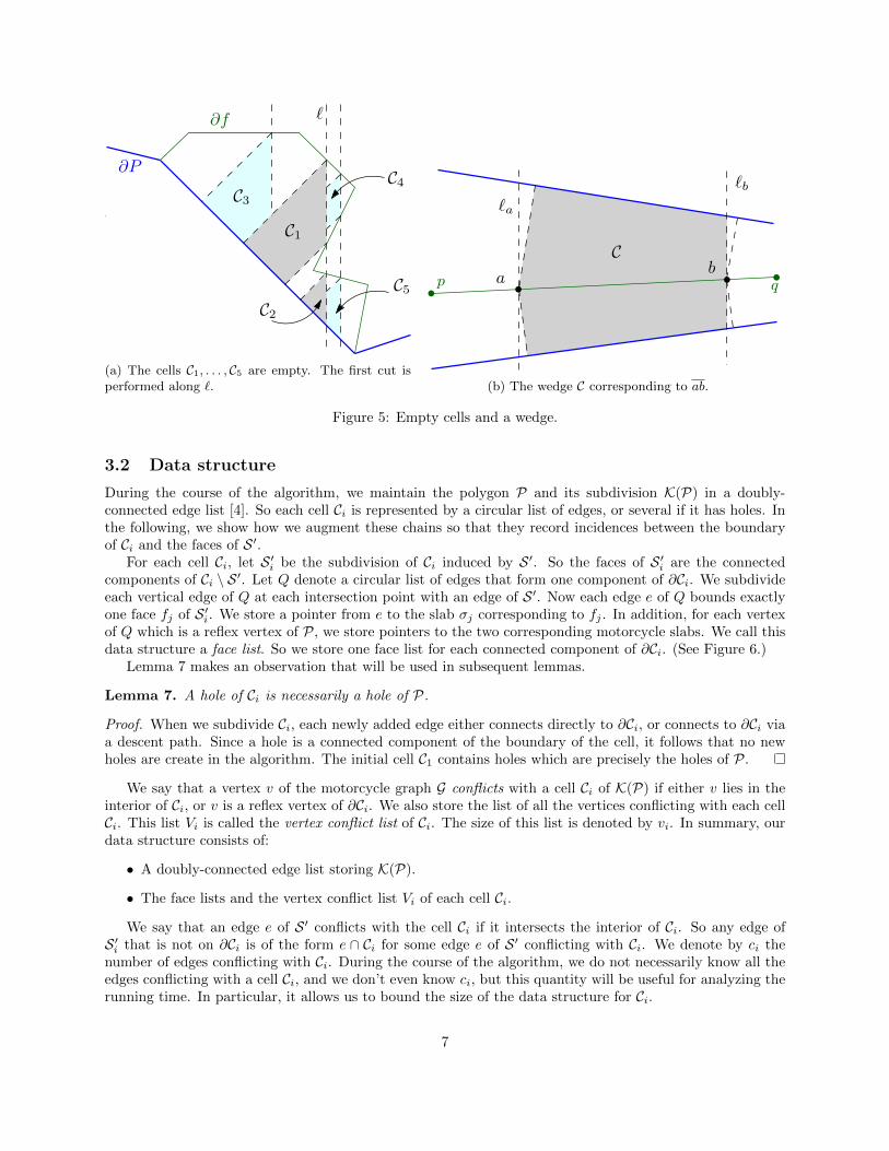
An empty cell is a cell of K(P) whose interior does not overlap with S ′. (See Figure 5a.) Thus an emptycell is entirely contained in a face of S ′. Another type of cell, called a wedge, will play an important rolein the analysis of our algorithm. Let pq be a ridge of S ′, and let a, b be two points in the interior of pq.Let `a and `b be the vertical lines through a and b, respectively. Consider the subdivision of P obtained byinserting vertical boundaries along `a and `b, and the four descent paths from a and b. (See Figure 5b.) Thecell of this subdivision containing ab is called the wedge corresponding to ab. The lemma below shows thatwedges are the only cells that can overlap the interior of a ridge, without enclosing any of its endpoints.

Lemma 6. Let Ci be a cell overlapping a ridge, but not its endpoints. Then Ci is a wedge.

Proof. Let a and b be the points on ∂Ci which are farthest along the ridge in either direction. A ridge canonly meet descent paths that start from it, so a and b must each lie on a vertical cut, `a and `b. No verticalcut has been made between a and b, otherwise a and b could not be in the same cell. So there is no verticalcut in the interior of the wedge corresponding to ab, and thus no descent path has been traced inside thiswedge. It follows that this wedge is Ci.

6

∂P

`∂f

C1

C2

C3C4

C5

(a) The cells C1, . . . , C5 are empty. The first cut isperformed along `.

`b

ab

p q

`a

C

(b) The wedge C corresponding to ab.

Figure 5: Empty cells and a wedge.

3.2 Data structure

During the course of the algorithm, we maintain the polygon P and its subdivision K(P) in a doubly-connected edge list [4]. So each cell Ci is represented by a circular list of edges, or several if it has holes. Inthe following, we show how we augment these chains so that they record incidences between the boundaryof Ci and the faces of S ′.

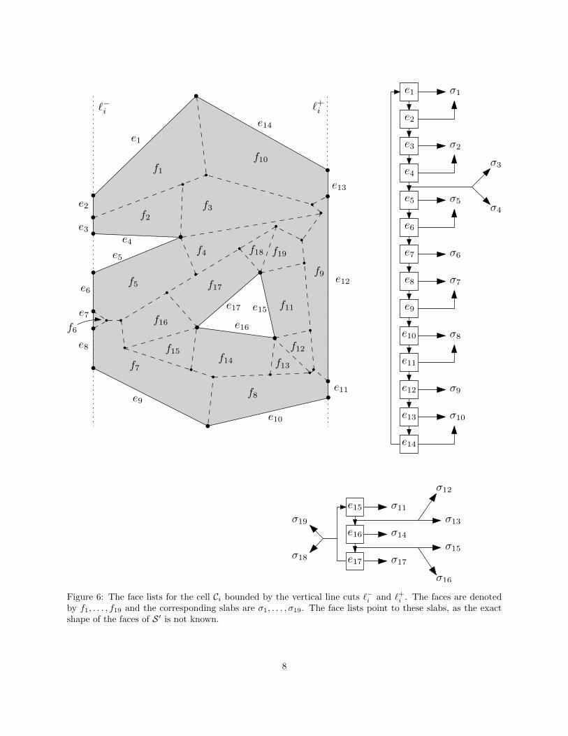
For each cell Ci, let S ′i be the subdivision of Ci induced by S ′. So the faces of S ′i are the connectedcomponents of Ci \ S ′. Let Q denote a circular list of edges that form one component of ∂Ci. We subdivideeach vertical edge of Q at each intersection point with an edge of S ′. Now each edge e of Q bounds exactlyone face fj of S ′i. We store a pointer from e to the slab σj corresponding to fj . In addition, for each vertexof Q which is a reflex vertex of P, we store pointers to the two corresponding motorcycle slabs. We call thisdata structure a face list. So we store one face list for each connected component of ∂Ci. (See Figure 6.)

Lemma 7 makes an observation that will be used in subsequent lemmas.

Lemma 7. A hole of Ci is necessarily a hole of P.

Proof. When we subdivide Ci, each newly added edge either connects directly to ∂Ci, or connects to ∂Ci viaa descent path. Since a hole is a connected component of the boundary of the cell, it follows that no newholes are create in the algorithm. The initial cell C1 contains holes which are precisely the holes of P.

We say that a vertex v of the motorcycle graph G conflicts with a cell Ci of K(P) if either v lies in theinterior of Ci, or v is a reflex vertex of ∂Ci. We also store the list of all the vertices conflicting with each cellCi. This list Vi is called the vertex conflict list of Ci. The size of this list is denoted by vi. In summary, ourdata structure consists of:

• A doubly-connected edge list storing K(P).

• The face lists and the vertex conflict list Vi of each cell Ci.

We say that an edge e of S ′ conflicts with the cell Ci if it intersects the interior of Ci. So any edge ofS ′i that is not on ∂Ci is of the form e ∩ Ci for some edge e of S ′ conflicting with Ci. We denote by ci thenumber of edges conflicting with Ci. During the course of the algorithm, we do not necessarily know all theedges conflicting with a cell Ci, and we don’t even know ci, but this quantity will be useful for analyzing therunning time. In particular, it allows us to bound the size of the data structure for Ci.

7

`+i`−i

e1

e2

e3e4

e5

e6

e7

e8

e9

e10

e11

e12

e13

e14

e17 e15

e16

f1

f2f3

f4

f5

f6

f7

f8

f9

f10

f19

f11

f12

f13f14

f15

f16

f17

f18

e1

e2

e3

e4

e5

e6

e7

e8

e9

e10

e11

e12

e13

e14

σ1

σ2

σ3

σ4σ5

σ6

σ7

σ8

σ9

σ10

e15

e16

e17

σ11

σ14

σ17

σ12

σ13

σ15

σ16

σ18

σ19

Figure 6: The face lists for the cell Ci bounded by the vertical line cuts `−i and `+i . The faces are denotedby f1, . . . , f19 and the corresponding slabs are σ1, . . . , σ19. The face lists point to these slabs, as the exactshape of the faces of S ′ is not known.

8

Lemma 8. If Ci is non-empty, then the total size of the face lists of Ci is O(ci). In particular, it impliesthat ∂Ci has O(ci) edges, and Ci overlaps O(ci) faces of S ′. On the other hand, if Ci is empty, then the totalsize is O(1), and thus ∂Ci has O(1) edges.

Proof. Let Q denote the outer boundary of Ci, and let |Q| denote its number of edges. By Lemma 3, eachreflex vertex p of Q is in a valley, and the two edges of Q incident to p bound the two faces of S ′i incidentto this valley. So any subchain Q′ of Q that bounds only one face f ′ of S ′i must be convex. The edges of Q′

can take only 3 directions: vertical, parallel to the base edge of f , or the steepest descent direction. So Q′

can have at most 5 edges: two vertical edges, two edges parallel to the steepest descent direction, and oneedge along the base edge of f ′.

Thus, Q can be partitioned into at least |Q|/5 subchains, such that two consecutive subchains bounddifferent faces. Any vertex of Q at which two consecutive subchains meet must be incident to an edge e ofS ′i that conflicts with Ci. By Lemma 4 and 5, this edge can meet ∂Ci at most twice. So in total, Q has atmost 10(ci + 1) edges.

Now consider the holes of Ci, if any. Such a hole must be a hole of P according to Lemma 7, so eachvertex along its boundary is the endpoint of at least one edge that conflicts with Ci. Each conflicting edge isadjacent to at most one hole vertex, so there are O(ci) such vertices in Ci. In addition, each edge of a holebounds only one face, and for each reflex vertex, another two faces corresponding to motorcycle slabs areadded. So in total, the face lists for holes have size O(ci).

We just proved that the total size of the face lists is O(ci + 1). If ci is non-empty, we have ci ≥ 1, andthus the bound can be written O(ci). Otherwise, if Ci is empty, then it does not conflict with any edge, soci = 0. Hence, the data structure has size O(1).

3.3 Algorithm

Our algorithm partitions P recursively, using vertical cuts, as in Sect. 3.1. In this section, we show how toperform a step of this subdivision in near-linear time. A cell Ci is subdivided along a vertical cut throughits median conflicting vertex, so the vertex conflict lists of the new cells will be at most half the size ofthe conflict lists of Ci. When the vertex conflict list of Ci is empty, we call the procedure Divide-Valleypresented in Section 4. If Ci is empty or is a wedge, then we stop subdividing Ci, and it becomes a leaf cell.

We now describe in more details how we perform this subdivision efficiently. We assume that the cell Ciconflicts with at least one vertex, and that Ci is given with the corresponding data structure as described inSect. 3.2. We first find the median conflicting vertex in time O(vi). We compute the list of vertical boundarysegments s1, . . . , sq created by the cut along the vertical line ` through the median vertex. This list is sortedalong `, and it can be constructed in time proportional to the number of edges bounding Ci, which is O(ci)by Lemma 8.

Then we compute the lifted polylines s1, . . . , sq as follows. Let H denote the vertical plane through `.We first find the list of slabs corresponding to the faces of S ′i. We obtain this list as the union of the slabsthat appear in the face lists of Ci. We compute the intersection of each such slab with H. This gives us a setof O(ci) segments in H, of which we compute the lower envelope. It can be done in O(ci log ci) time usingan algorithm by Hershberger [20]. Then we obtain s1, . . . , sq by scanning through this lower envelope andthe list s1, . . . , sq. Overall it takes time O(ci log ci) to compute this lower envelope, and it has O(ci) edges,as each edge of S ′i or Ci creates at most one vertex along this chain.

The partition induced by ` is obtained by tracing steepest descent paths from s1, . . . , sq. For a verticaledge sj , any point where sj changes direction, when projected onto the horizontal plane, corresponds preciselyto a point where sj intersects an edge e of S ′i. At each of these points, we do the following without actuallyknowing S ′i. There are at most three steepest descent paths from a = e ∩ sj , one for each slab through a.Each such descent path consists of one line segment along the slab, followed possibly by another line segmentalong a valley in the case where the slab is a motorcycle slab. Let γ denote one of these descent paths. Aswe know the slab and the starting point of γ, we can construct γ in constant time. This path γ goes all theway to ∂P, so if necessary, we clip it at `−i or `+i to obtain its restriction to Ci.

9

These descent paths cannot cross, and by construction they do not cross the vertical boundary edges.Each edge of S ′i may create at most three such descent paths, so we create O(ci) such new descent paths.There are also O(ci) new vertical edges, so we can update the doubly-connected edge list in time O(ci log ci)by plane sweep. Using an additional O(vi log ci) time, we can update the vertex conflict lists during thisplane sweep. The face lists can be updated in overall O(ci) time by splitting the face lists of Ci along thelower endpoints of the new descent paths, and inserting new subchains along each vertical edge sj , which weobtain directly from sj in linear time. So we just proved the following:

Lemma 9. We can compute the subdivision of a non-empty cell Ci induced by a line through its medianconflicting vertex, and update our data structure accordingly, in O((ci + vi) log ci) time.

Algorithm 1 Vertical subdivision

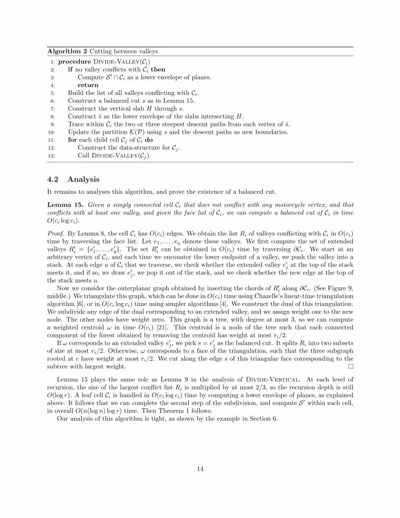
1: procedure Divide-Vertical(Ci)2: Select median vertex in Vi, and draw the vertical line ` through it.3: Construct the vertical edges s1, . . . , sq of ` ∩ Ci.4: Compute the lower envelope of the slabs along the vertical plane through `.5: Construct the lifted version s1, . . . , sq of the vertical boundary segments.6: Trace within Ci the steepest descent paths from each vertex of s1, . . . , sq.7: Update K(P) using s1, . . . , sq and the descent paths as new boundaries.8: for each child cell Cj of Ci do9: Construct the data structure for Cj .

10: if Cj is a wedge or is empty then11: Compute S ′j by brute force.12: else13: if Vj = ∅ then14: Call Divide-Valley(Ci)15: else16: Call Divide-Vertical(Cj).

3.4 Analysis

In the previous section, we saw that the vertical subdivision of each cell Ci can be obtained in time near-linearin the size of the data structure for Ci. We now bound the overall running time of the algorithm, so we needto bound the sum

∑i ci + vi over all cells created by Divide-Vertical.

We use the recursion tree associated with Algorithm 1. Each node ν of this tree represents a cell Ci, andthe child cells of Ci are stored at the descendants of ν in the recursion tree. In particular, the cells stored atthe descendants of ν form a partition of the cell stored at ν. Each time we subdivide a cell Ci, the conflictlist of each new cell has at most half the size of the conflict list of Ci. As there are at most 2r vertices in G,it follows that:

Lemma 10. The recursion tree of Divide-Vertical has depth O(log r).

The degree of any vertex in K(P) is at most 5, because there can be at most three descent paths throughany point, as well as two vertical edges. It implies that any point of P is contained in at most 5 cells at eachlevel of the recursion tree. It follows that:

Lemma 11. Any point in P is contained in O(log r) cells of K(P) throughout the algorithm.

In particular, if we apply this result to each of the 2r vertices of G, we obtain:

Lemma 12. Throughout the algorithm, the sum∑

i vi of the sizes of the vertex conflict lists is O(r log r).

10

p

q

a

b

p

q

a

b

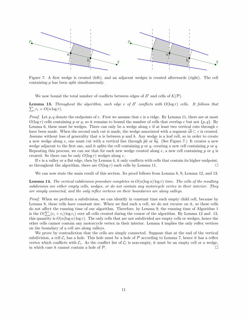
Figure 7: A first wedge is created (left), and an adjacent wedges is created afterwards (right). The cellcontaining p has been split simultaneously.

We now bound the total number of conflicts between edges of S ′ and cells of K(P).

Lemma 13. Throughout the algorithm, each edge e of S ′ conflicts with O(log r) cells. It follows that∑i ci = O(n log r).

Proof. Let p, q denote the endpoints of e. First we assume that e is a ridge. By Lemma 11, there are at mostO(log r) cells containing p or q, so it remains to bound the number of cells that overlap e but not p, q. ByLemma 6, these must be wedges. There can only be a wedge along e if at least two vertical cuts through ehave been made. When the second such cut is made, the wedge associated with a segment ab ⊂ e is created.Assume without loss of generality that a is between p and b. Any wedge is a leaf cell, so in order to createa new wedge along e, one must cut with a vertical line through pa or bq. (See Figure 7.) It creates a newwedge adjacent to the first one, and it splits the cell containing p or q, creating a new cell containing p or q.Repeating this process, we can see that for each new wedge created along e, a new cell containing p or q iscreated. So there can be only O(log r) wedges along e.

If e is a valley or a flat edge, then by Lemma 4, it only conflicts with cells that contain its higher endpoint,so throughout the algorithm, there are O(log r) such cells by Lemma 11.

We can now state the main result of this section. Its proof follows from Lemma 8, 9, Lemma 12, and 13.

Lemma 14. The vertical subdivision procedure completes in O(n(log n) log r) time. The cells of the resultingsubdivision are either empty cells, wedges, or do not contain any motorcycle vertex in their interior. Theyare simply connected, and the only reflex vertices on their boundaries are along valleys.

Proof. When we perform a subdivision, we can identify in constant time each empty child cell, because byLemma 8, these cells have constant size. When we find such a cell, we do not recurse on it, so these cellsdo not affect the running time of our algorithm. Therefore, by Lemma 9, the running time of Algorithm 1is the O(

∑i(ci + vi) log ci) over all cells created during the course of the algorithm. By Lemma 12 and 13,

this quantity is O(n(log n) log r). The only cells that are not subdivided are empty cells or wedges, hence theother cells cannot contain any motorcycle vertex in their interior. Lemma 4 implies the only reflex verticeson the boundary of a cell are along valleys.

We prove by contradiction that the cells are simply connected. Suppose that at the end of the verticalsubdivision, a cell Ci has a hole. This hole must be a hole of P according to Lemma 7, hence it has a reflexvertex which conflicts with Ci. As the conflict list of Ci is non-empty, it must be an empty cell or a wedge,in which case it cannot contain a hole of P.

11

(a) Input polygon and straight skeleton. (b) First vertical cut.

(c) Subdivision induced by the first vertical cut. (d) Second vertical cut.

(e) Subdivision induced by the second vertical cut. (f) Third vertical cut.

Figure 8: The vertical subdivision. (Continued in Figure 10.)

12

CiCi

s

Ci

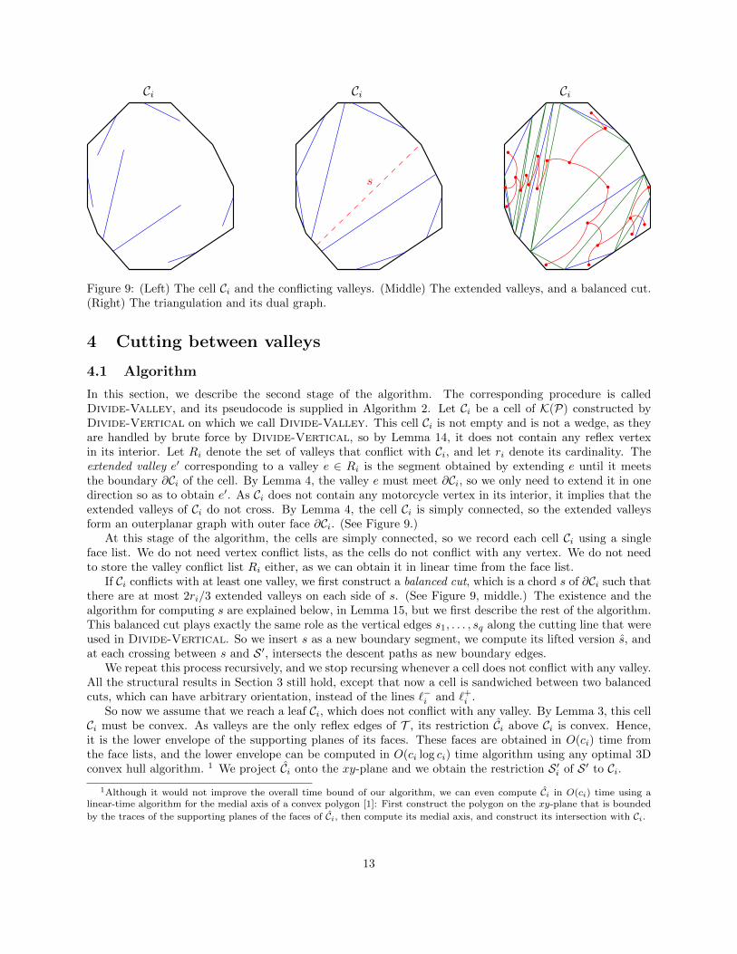
Figure 9: (Left) The cell Ci and the conflicting valleys. (Middle) The extended valleys, and a balanced cut.(Right) The triangulation and its dual graph.

4 Cutting between valleys

4.1 Algorithm

In this section, we describe the second stage of the algorithm. The corresponding procedure is calledDivide-Valley, and its pseudocode is supplied in Algorithm 2. Let Ci be a cell of K(P) constructed byDivide-Vertical on which we call Divide-Valley. This cell Ci is not empty and is not a wedge, as theyare handled by brute force by Divide-Vertical, so by Lemma 14, it does not contain any reflex vertexin its interior. Let Ri denote the set of valleys that conflict with Ci, and let ri denote its cardinality. Theextended valley e′ corresponding to a valley e ∈ Ri is the segment obtained by extending e until it meetsthe boundary ∂Ci of the cell. By Lemma 4, the valley e must meet ∂Ci, so we only need to extend it in onedirection so as to obtain e′. As Ci does not contain any motorcycle vertex in its interior, it implies that theextended valleys of Ci do not cross. By Lemma 4, the cell Ci is simply connected, so the extended valleysform an outerplanar graph with outer face ∂Ci. (See Figure 9.)

At this stage of the algorithm, the cells are simply connected, so we record each cell Ci using a singleface list. We do not need vertex conflict lists, as the cells do not conflict with any vertex. We do not needto store the valley conflict list Ri either, as we can obtain it in linear time from the face list.

If Ci conflicts with at least one valley, we first construct a balanced cut, which is a chord s of ∂Ci such thatthere are at most 2ri/3 extended valleys on each side of s. (See Figure 9, middle.) The existence and thealgorithm for computing s are explained below, in Lemma 15, but we first describe the rest of the algorithm.This balanced cut plays exactly the same role as the vertical edges s1, . . . , sq along the cutting line that wereused in Divide-Vertical. So we insert s as a new boundary segment, we compute its lifted version s, andat each crossing between s and S ′, intersects the descent paths as new boundary edges.

We repeat this process recursively, and we stop recursing whenever a cell does not conflict with any valley.All the structural results in Section 3 still hold, except that now a cell is sandwiched between two balancedcuts, which can have arbitrary orientation, instead of the lines `−i and `+i .

So now we assume that we reach a leaf Ci, which does not conflict with any valley. By Lemma 3, this cellCi must be convex. As valleys are the only reflex edges of T , its restriction Ci above Ci is convex. Hence,it is the lower envelope of the supporting planes of its faces. These faces are obtained in O(ci) time fromthe face lists, and the lower envelope can be computed in O(ci log ci) time algorithm using any optimal 3Dconvex hull algorithm. 1 We project Ci onto the xy-plane and we obtain the restriction S ′i of S ′ to Ci.

1Although it would not improve the overall time bound of our algorithm, we can even compute Ci in O(ci) time using alinear-time algorithm for the medial axis of a convex polygon [1]: First construct the polygon on the xy-plane that is bounded

by the traces of the supporting planes of the faces of Ci, then compute its medial axis, and construct its intersection with Ci.

13

Algorithm 2 Cutting between valleys

1: procedure Divide-Valley(Ci)2: if no valley conflicts with Ci then3: Compute S ′ ∩ Ci as a lower envelope of planes.4: return5: Build the list of all valleys conflicting with Ci.6: Construct a balanced cut s as in Lemma 15.7: Construct the vertical slab H through s.8: Construct s as the lower envelope of the slabs intersecting H.9: Trace within Ci the two or three steepest descent paths from each vertex of s.

10: Update the partition K(P) using s and the descent paths as new boundaries.11: for each child cell Cj of Ci do12: Construct the data-structure for Cj .13: Call Divide-Valley(Cj).

4.2 Analysis

It remains to analyses this algorithm, and prove the existence of a balanced cut.

Lemma 15. Given a simply connected cell Ci that does not conflict with any motorcycle vertex, and thatconflicts with at least one valley, and given the face list of Ci, we can compute a balanced cut of Ci in timeO(ci log ci).

Proof. By Lemma 8, the cell Ci has O(ci) edges. We obtain the list Ri of valleys conflicting with Ci in O(ci)time by traversing the face list. Let e1, . . . , eq denote these valleys. We first compute the set of extendedvalleys R′i = e′1, . . . , e′q. The set R′i can be obtained in O(ci) time by traversing ∂Ci. We start at anarbitrary vertex of Ci, and each time we encounter the lower endpoint of a valley, we push the valley into astack. At each edge u of Ci that we traverse, we check whether the extended valley e′j at the top of the stackmeets it, and if so, we draw e′j , we pop it out of the stack, and we check whether the new edge at the top ofthe stack meets u.

Now we consider the outerplanar graph obtained by inserting the chords of R′i along ∂Ci. (See Figure 9,middle.) We triangulate this graph, which can be done inO(ci) time using Chazelle’s linear-time triangulationalgorithm [6], or in O(ci log ci) time using simpler algorithms [4]. We construct the dual of this triangulation.We subdivide any edge of the dual corresponding to an extended valley, and we assign weight one to the newnode. The other nodes have weight zero. This graph is a tree, with degree at most 3, so we can computea weighted centroid ω in time O(ci) [21]. This centroid is a node of the tree such that each connectedcomponent of the forest obtained by removing the centroid has weight at most ri/2.

If ω corresponds to an extended valley e′j , we pick s = e′j as the balanced cut. It splits Ri into two subsetsof size at most ri/2. Otherwise, ω corresponds to a face of the triangulation, such that the three subgraphrooted at c have weight at most ri/2. We cut along the edge s of this triangular face corresponding to thesubtree with largest weight.

Lemma 15 plays the same role as Lemma 9 in the analysis of Divide-Vertical. At each level ofrecursion, the size of the largest conflict list Ri is multiplied by at most 2/3, so the recursion depth is stillO(log r). A leaf cell Ci is handled in O(ci log ci) time by computing a lower envelope of planes, as explainedabove. It follows that we can complete the second step of the subdivision, and compute S ′ within each cell,in overall O(n(log n) log r) time. Then Theorem 1 follows.

Our analysis of this algorithm is tight, as shown by the example in Section 6.

14

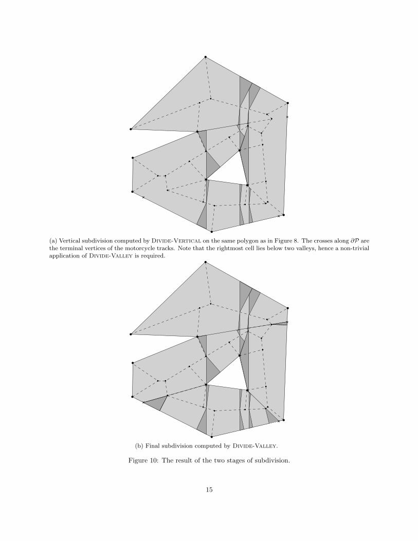
(a) Vertical subdivision computed by Divide-Vertical on the same polygon as in Figure 8. The crosses along ∂P arethe terminal vertices of the motorcycle tracks. Note that the rightmost cell lies below two valleys, hence a non-trivialapplication of Divide-Valley is required.

(b) Final subdivision computed by Divide-Valley.

Figure 10: The result of the two stages of subdivision.

15

a

b

c

d

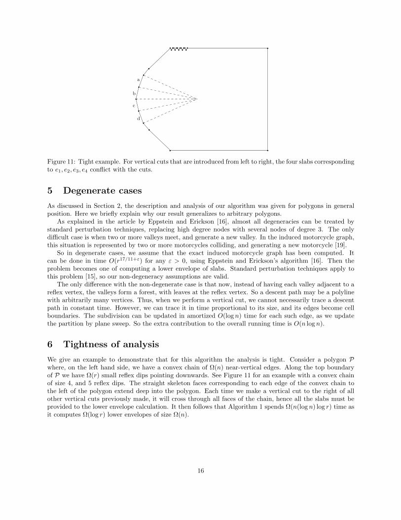
Figure 11: Tight example. For vertical cuts that are introduced from left to right, the four slabs correspondingto e1, e2, e3, e4 conflict with the cuts.

5 Degenerate cases

As discussed in Section 2, the description and analysis of our algorithm was given for polygons in generalposition. Here we briefly explain why our result generalizes to arbitrary polygons.

As explained in the article by Eppstein and Erickson [16], almost all degeneracies can be treated bystandard perturbation techniques, replacing high degree nodes with several nodes of degree 3. The onlydifficult case is when two or more valleys meet, and generate a new valley. In the induced motorcycle graph,this situation is represented by two or more motorcycles colliding, and generating a new motorcycle [19].

So in degenerate cases, we assume that the exact induced motorcycle graph has been computed. Itcan be done in time O(r17/11+ε) for any ε > 0, using Eppstein and Erickson’s algorithm [16]. Then theproblem becomes one of computing a lower envelope of slabs. Standard perturbation techniques apply tothis problem [15], so our non-degeneracy assumptions are valid.

The only difference with the non-degenerate case is that now, instead of having each valley adjacent to areflex vertex, the valleys form a forest, with leaves at the reflex vertex. So a descent path may be a polylinewith arbitrarily many vertices. Thus, when we perform a vertical cut, we cannot necessarily trace a descentpath in constant time. However, we can trace it in time proportional to its size, and its edges become cellboundaries. The subdivision can be updated in amortized O(log n) time for each such edge, as we updatethe partition by plane sweep. So the extra contribution to the overall running time is O(n log n).

6 Tightness of analysis

We give an example to demonstrate that for this algorithm the analysis is tight. Consider a polygon Pwhere, on the left hand side, we have a convex chain of Ω(n) near-vertical edges. Along the top boundaryof P we have Ω(r) small reflex dips pointing downwards. See Figure 11 for an example with a convex chainof size 4, and 5 reflex dips. The straight skeleton faces corresponding to each edge of the convex chain tothe left of the polygon extend deep into the polygon. Each time we make a vertical cut to the right of allother vertical cuts previously made, it will cross through all faces of the chain, hence all the slabs must beprovided to the lower envelope calculation. It then follows that Algorithm 1 spends Ω(n(log n) log r) time asit computes Ω(log r) lower envelopes of size Ω(n).

16

References

[1] A. Aggarwal, L. J. Guibas, J. Saxe, and P. W. Shor. A linear-time algorithm for computing the voronoidiagram of a convex polygon. Discrete and Computational Geometry, 4(1):591–604, 1989.

[2] O. Aichholzer, D. Alberts, F. Aurenhammer, and B. Gartner. A novel type of skeleton for polygons.Journal of Universal Computer Science, 1(12):752–761, 1995.

[3] G. Barequet, M. Goodrich, A. Levi-Steiner, and D. Steiner. Straight-skeleton based contour interpo-lation. Proceedings of the 14th annual ACM-SIAM symposium on Discrete algorithms, pages 119–127,2003.

[4] Mark de Berg, Otfried Cheong, Marc van Kreveld, and Mark Overmars. Computational Geometry:Algorithms and Applications. Springer-Verlag, 2008.

[5] J. Bowers. Computing the straight skeleton of a simple polygon from its motorcycle graph in determin-istic O(n log n) time. CoRR, abs/1405.6260, 2014.

[6] B. Chazelle. Triangulating a simple polygon in linear time. Discrete Comput. Geom., 6(5):485–524,August 1991.

[7] S.-W. Cheng and A. Vigneron. Motorcycle graphs and straight skeletons. Algorithmica, 47(2):159–182,2007.

[8] F. Chin, J. Snoeyink, and C. A. Wang. Finding the medial axis of a simple polygon in linear time.Discrete and Computational Geometry, 21(3):405–420, 1999.

[9] F. Cloppet, J. Oliva, and G. Stamon. Angular bisector network, a simplified generalized voronoi diagram:Application to processing complex intersections in biomedical images. IEEE Transactions on PatternAnalysis and Machine Intelligence, 22(1):120–128, 2000.

[10] S. Coquillart, J. Oliva, and M. Perrin. 3d reconstruction of complex polyhedral shapes from contoursusing a simplified generalized voronoi diagram. Computer Graphics Forum, 15(3):397–408, 1996.

[11] A. Day and R. Laycock. Automatically generating large urban environments based on the footprintdata of buildings. Proceedings of the 8th ACM symposium on Solid Modeling and Applications, pages346–351, 2003.

[12] E. D. Demaine, M. L. Demaine, and A. Lubiw. Folding and cutting paper. Revised Papers from theJapan Conference on Discrete and Computational Geometry, pages 104–117, 1998.

[13] E. D. Demaine, M. L. Demaine, and A. Lubiw. Folding and one straight cut suffice. Proceedings of the10th Annual ACM-SIAM Symposium on Discrete Algorithms, pages 891–892, 1999.

[14] E. D. Demaine, M. L. Demaine, and J. S. B. Mitchell. Folding flat silhouettes and wrapping polyhedralpackages: New results in computational origami. Proceedings of the 15th Annual ACM Symposium onComputational Geometry, pages 105–114, 1999.

[15] H. Edelsbrunner and E. P. Mucke. Simulation of simplicity: A technique to cope with degenerate casesin geometric algorithms. ACM Trans. Graph., 9(1):66–104, 1990.

[16] D. Eppstein and J. Erickson. Raising roofs, crashing cycles, and playing pool: Applications of a datastructure for finding pairwise interactions. Discrete and Computational Geometry, 22(4):569–592, 1999.

[17] P. Felkel and S. Obdrzalek. Straight skeleton implementation. Proceedings of the 14th Spring Conferenceon Computer Graphics, pages 210–218, 1998.

17

[18] M. Held and S. Huber. Theoretical and practical results on straight skeletons of planar straight-linegraphs. Proceedings of the 27th Symposium on Computational Geometry, pages 171–178, 2011.

[19] M. Held and S. Huber. A fast straight-skeleton algorithm based on generalized motorcycle graphs.International Journal of Computational Geometry and Applications, 22(5):471–498, 2012.

[20] J. Hershberger. Finding the upper envelope of n line segments in O(n log n) time. Information ProcessingLetters, 33(4):169–174, 1989.

[21] O. Kariv and S. Hakimi. An algorithmic approach to network location problems. II: The p-medians.SIAM Journal on Applied Mathematics, 37(3):539–560, 1979.

[22] T. Kelly and P. Wonka. Interactive architectural modeling with procedural extrusions. ACM Transac-tions on Graphics, 30(2):14:1–14:15, 2011.

[23] A. Vigneron and L. Yan. A faster algorithm for computing motorcycle graphs. Proceedings of the 29thSymposium on Computational Geometry, pages 17–26, 2013.

[24] G. von Peschka. Kotirte Ebenen: Kotirte Projektionen und deren Anwendung; Vortrage. Brno: Buschakand Irrgang, 1877.

18