Siti Nor Jannah bt AhmadSiti Shahida bt Kamel

Zamriyah bt Abu Samah

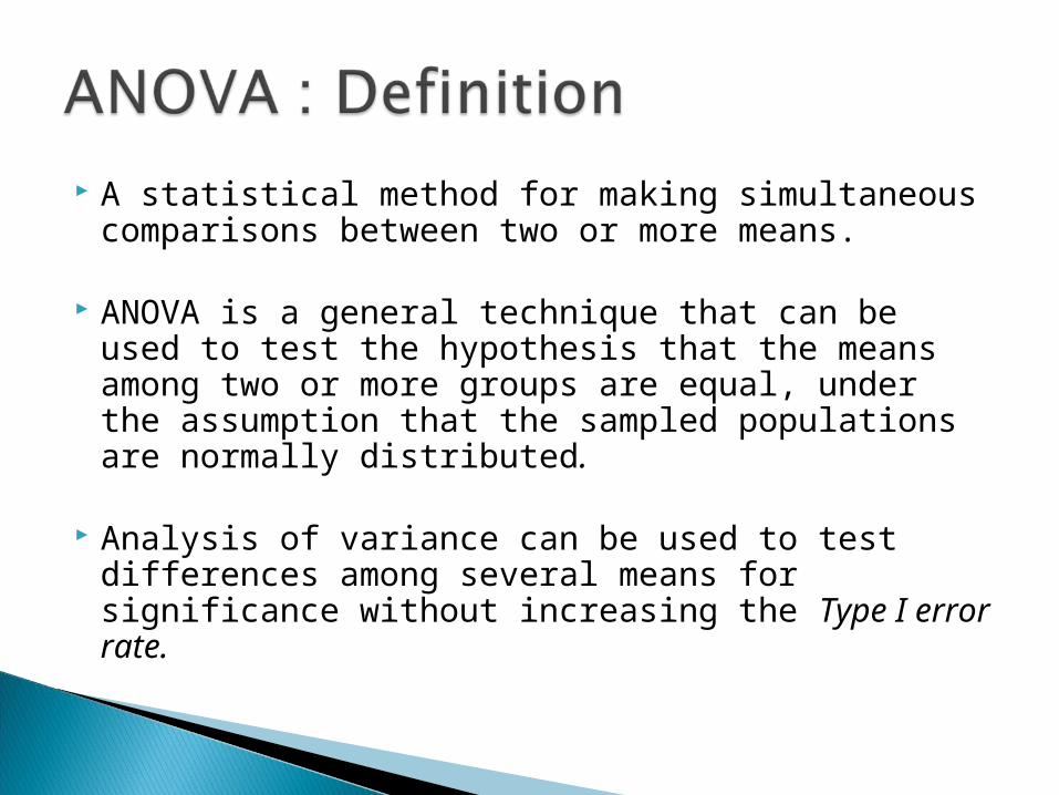
A statistical method for making simultaneous comparisons between two or more means.

ANOVA is a general technique that can be used to test the hypothesis that the means among two or more groups are equal, under the assumption that the sampled populations are normally distributed.

Analysis of variance can be used to test differences among several means for significance without increasing the Type I error rate.

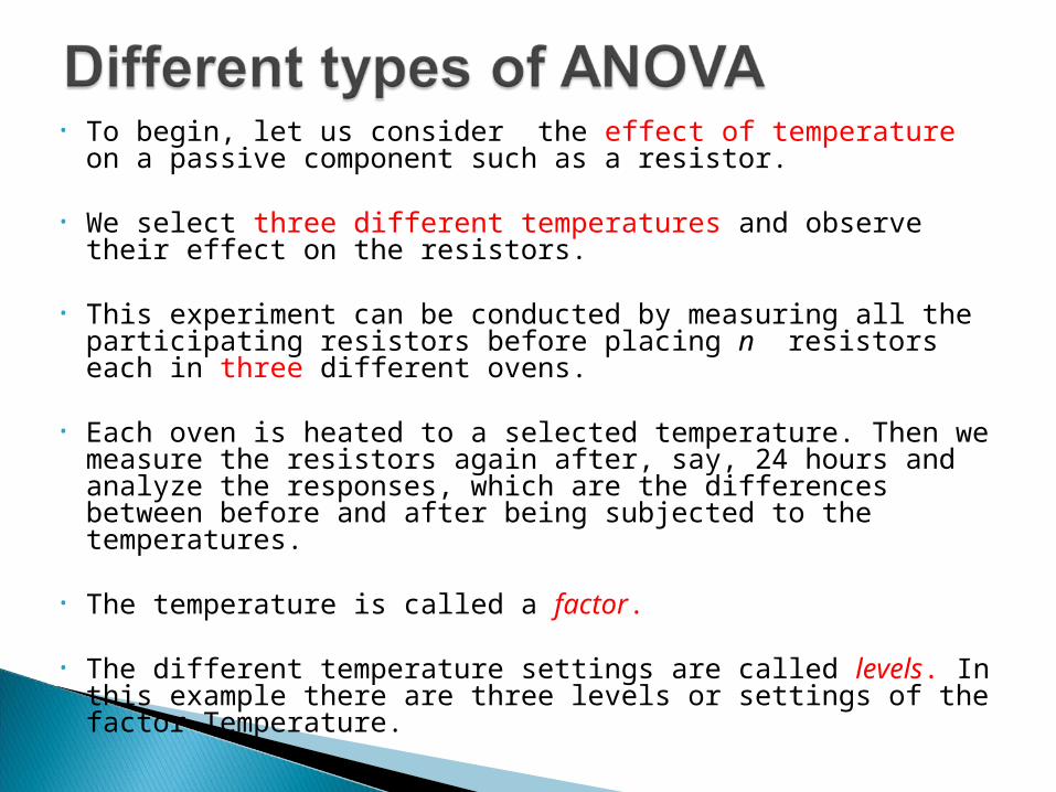
• To begin, let us consider the effect of temperature on a passive component such as a resistor.

• We select three different temperatures and observe their effect on the resistors.

• This experiment can be conducted by measuring all the participating resistors before placing n resistors each in three different ovens.

• Each oven is heated to a selected temperature. Then we measure the resistors again after, say, 24 hours and analyze the responses, which are the differences between before and after being subjected to the temperatures.

• The temperature is called a factor.

• The different temperature settings are called levels. In this example there are three levels or settings of the factor Temperature.

4

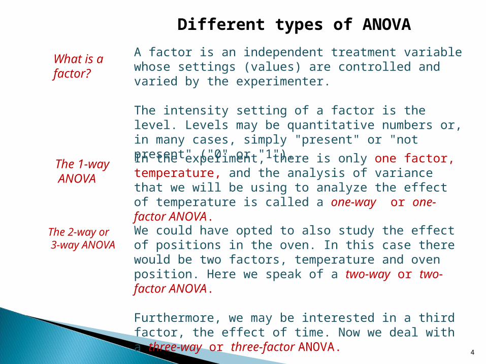
What is a factor?

A factor is an independent treatment variable whose settings (values) are controlled and varied by the experimenter.

The intensity setting of a factor is the level. Levels may be quantitative numbers or, in many cases, simply "present" or "not present" ("0" or "1").

In the experiment, there is only one factor, temperature, and the analysis of variance that we will be using to analyze the effect of temperature is called a one-way or one-factor ANOVA.

The 1-way ANOVA

The 2-way or 3-way ANOVA

We could have opted to also study the effect of positions in the oven. In this case there would be two factors, temperature and oven position. Here we speak of a two-way or two-factor ANOVA.

Furthermore, we may be interested in a third factor, the effect of time. Now we deal with a three-way or three-factor ANOVA.

Different types of ANOVA

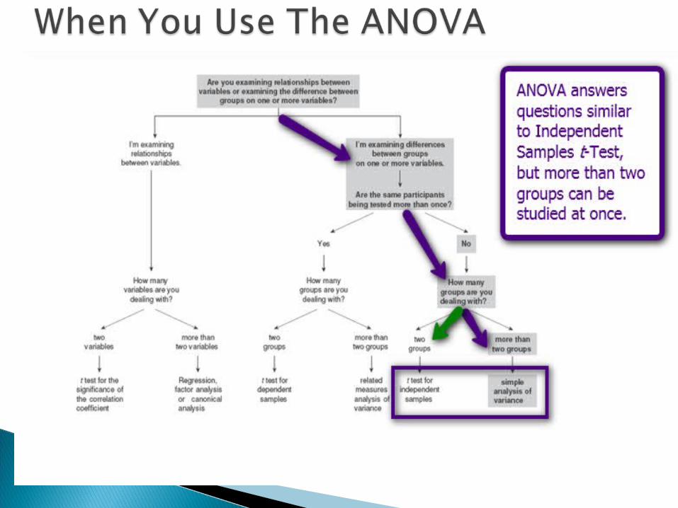
You may use ANOVA whenever you have 2 or more independent groups

You must use ANOVA whenever you have 3 or more independent groups.

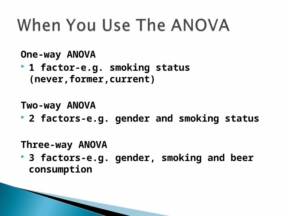
One-way ANOVA 1 factor-e.g. smoking status

(never,former,current)

Two-way ANOVA 2 factors-e.g. gender and smoking status

Three-way ANOVA 3 factors-e.g. gender, smoking and beer

consumption

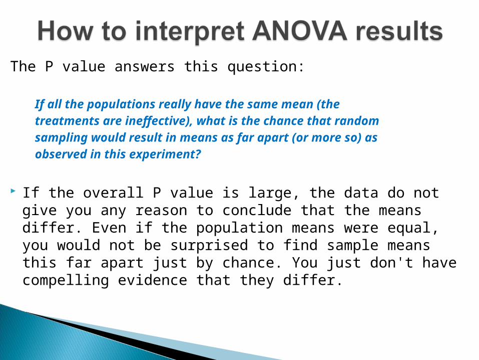
The P value answers this question:

If all the populations really have the same mean (thetreatments are ineffective), what is the chance that randomsampling would result in means as far apart (or more so) asobserved in this experiment?

If the overall P value is large, the data do not give you any reason to conclude that the means differ. Even if the population means were equal, you would not be surprised to find sample means this far apart just by chance. You just don't have compelling evidence that they differ.

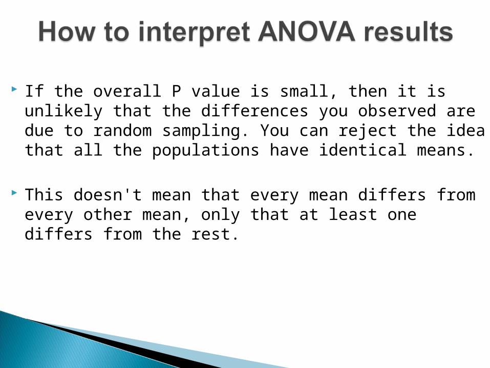
If the overall P value is small, then it is unlikely that the differences you observed are due to random sampling. You can reject the idea that all the populations have identical means.

This doesn't mean that every mean differs from every other mean, only that at least one differs from the rest.

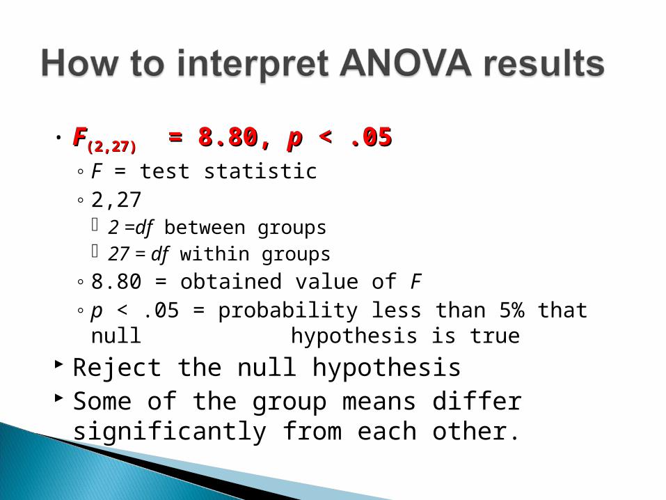
• FF(2,27)(2,27) = 8.80, = 8.80, pp < .05 < .05◦ F = test statistic ◦ 2,27

2 =df between groups 27 = df within groups

◦ 8.80 = obtained value of F ◦ p < .05 = probability less than 5% that null

hypothesis is true Reject the null hypothesis Some of the group means differ significantly from

each other.

Example◦ An apple juice manufacturer is planning to develop

a new product -a liquid concentrate.◦ The marketing manager has to decide how to

market the new product.◦ Three strategies are considered

Emphasize convenience of using the product. Emphasize the quality of the product. Emphasize the product’s low price.

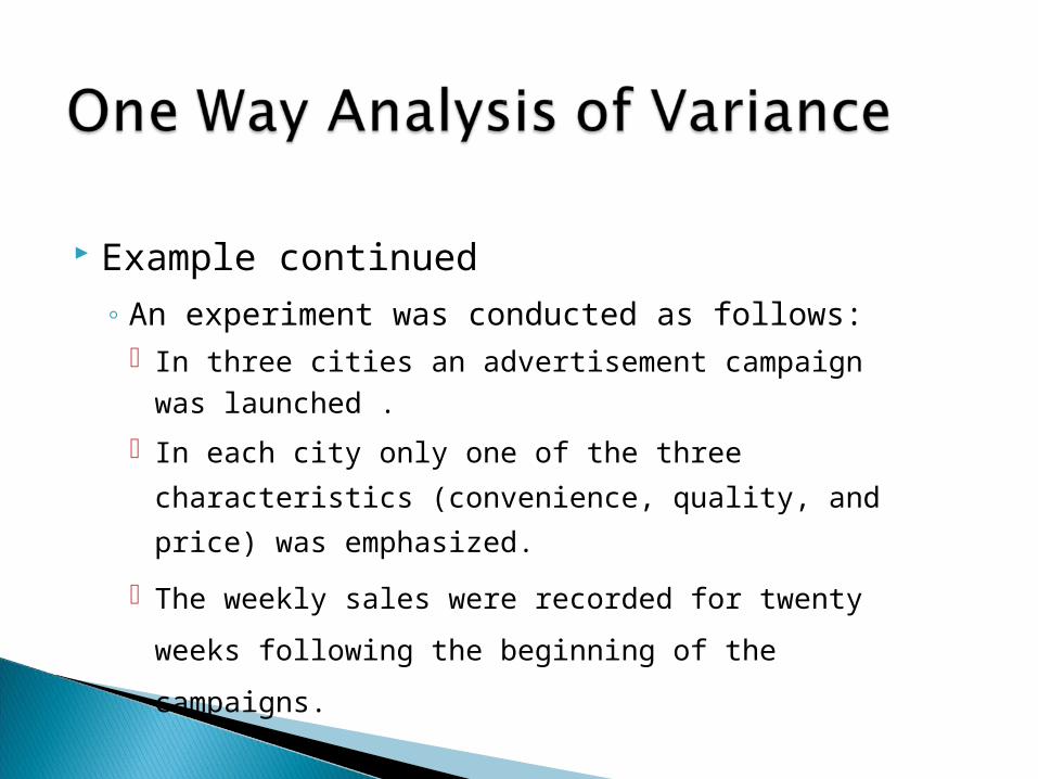
Example continued◦ An experiment was conducted as follows:

In three cities an advertisement campaign was launched .

In each city only one of the three characteristics

(convenience, quality, and price) was

emphasized.

The weekly sales were recorded for twenty weeks

following the beginning of the campaigns.

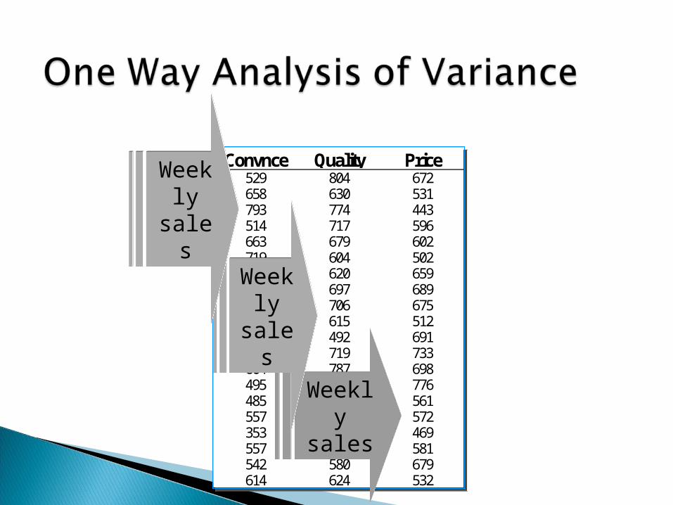
Convnce Quality Price529 804 672658 630 531793 774 443514 717 596663 679 602719 604 502711 620 659606 697 689461 706 675529 615 512498 492 691663 719 733604 787 698495 699 776485 572 561557 523 572353 584 469557 634 581542 580 679614 624 532

Convnce Quality Price529 804 672658 630 531793 774 443514 717 596663 679 602719 604 502711 620 659606 697 689461 706 675529 615 512498 492 691663 719 733604 787 698495 699 776485 572 561557 523 572353 584 469557 634 581542 580 679614 624 532

Weekly sales

Weekly

sales

Weekly

sales

In the context of this problem…Response variable – weekly salesResponses – actual sale valuesExperimental unit – weeks in the three cities when we record sales figures.Factor – the criterion by which we classify the populations (the treatments). In this problems the factor is the marketing strategy.Factor levels – the population (treatment) names. In this problem factor levels are the marketing strategies.

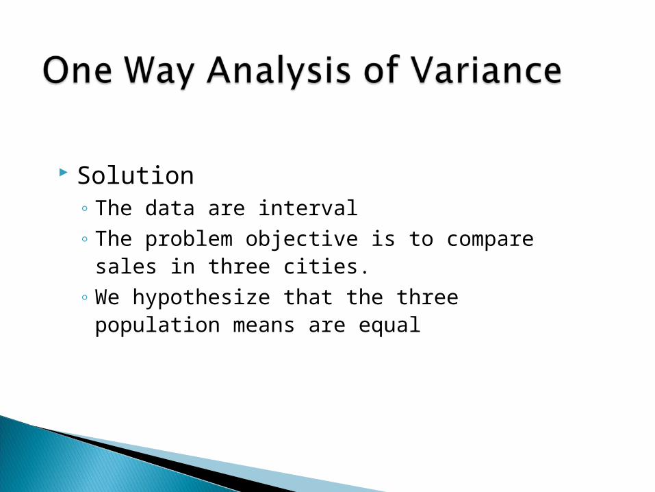
Solution◦ The data are interval◦ The problem objective is to compare sales in

three cities.◦ We hypothesize that the three population

means are equal

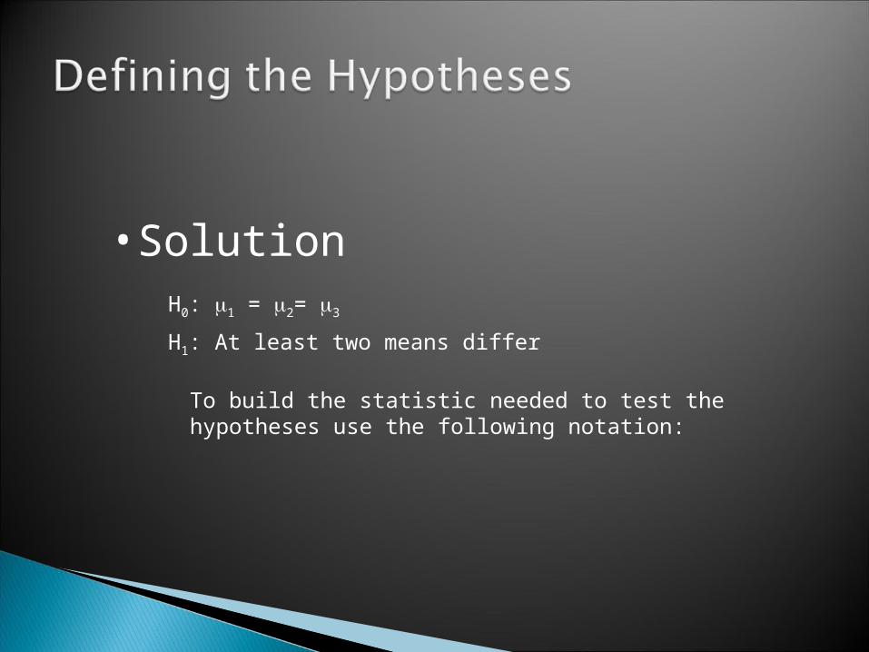
H0: 1 = 2= 3

H1: At least two means differ

To build the statistic needed to test thehypotheses use the following notation:

•Solution

If the null hypothesis is true, we would expect all the sample means to be close to one another (and as a result, close to the grand mean).

If the alternative hypothesis is true, at least some of the sample means would differ.

Thus, we measure variability between sample means.

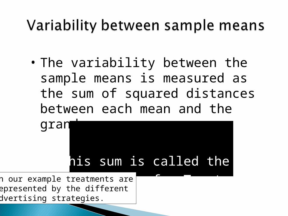
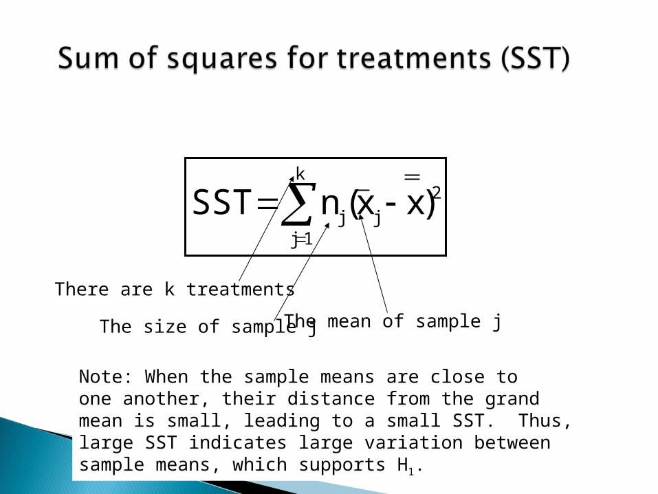
• The variability between the sample means is measured as the sum of squared distances between each mean and the grand mean.

This sum is called the Sum of Squares for Treatments

SSTIn our example treatments arerepresented by the differentadvertising strategies.

2k

1jjj )xx(nSST

There are k treatments

The size of sample j The mean of sample j

Note: When the sample means are close toone another, their distance from the grand mean is small, leading to a small SST. Thus, large SST indicates large variation between sample means, which supports H1.

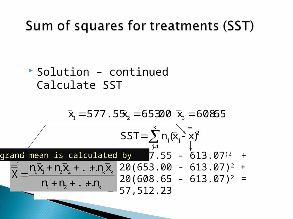
Solution – continuedCalculate SST

2k

1jjj

321

)xx(nSST

65.608x00.653x577.55x

= 20(577.55 - 613.07)2 + + 20(653.00 - 613.07)2 + + 20(608.65 - 613.07)2 == 57,512.23

The grand mean is calculated by

k21

kk2211

n...nnxn...xnxn

X

Large variability within the samples weakens the “ability” of the sample means to represent their corresponding population means.

Therefore, even though sample means may markedly differ from one another, SST must be judged relative to the “within samples variability”.

The variability within samples is measured by adding all the squared distances between observations and their sample means.

This sum is called the Sum of Squares for Error

SSEIn our example this is the sum of all squared differencesbetween sales in city j and thesample mean of city j (over all the three cities).

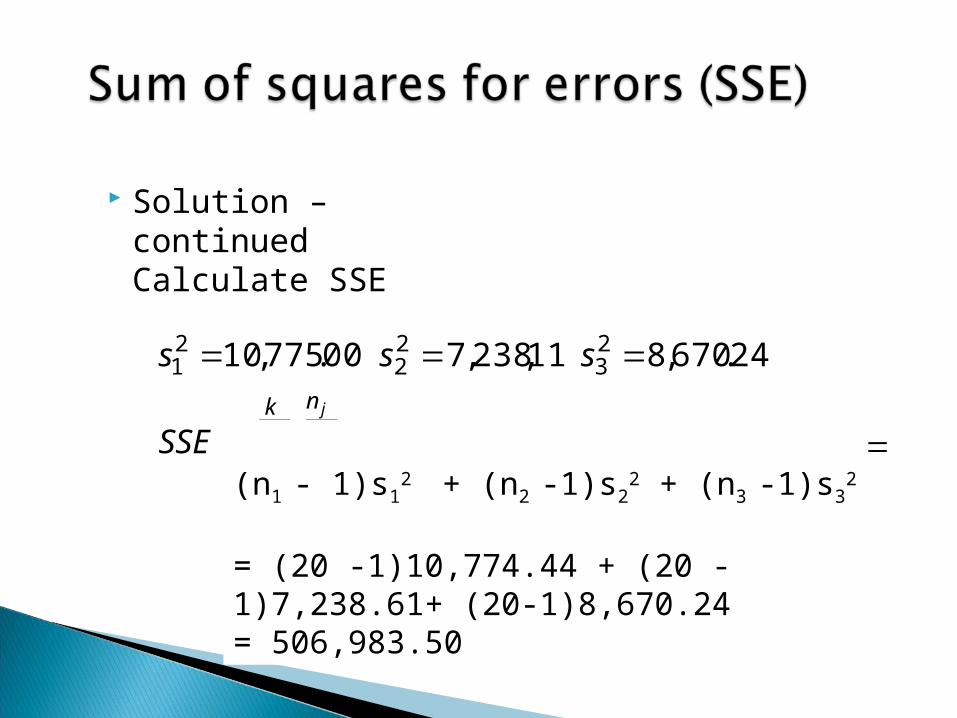
Solution – continuedCalculate SSE

k

jjij

n

i

xxSSE

sss

j

1

2

1

23

22

21

)(

24.670,811,238,700.775,10

(n1 - 1)s12 + (n2 -

1)s22 + (n3 -1)s3

2

= (20 -1)10,774.44 + (20 -1)7,238.61+ (20-1)8,670.24 = 506,983.50

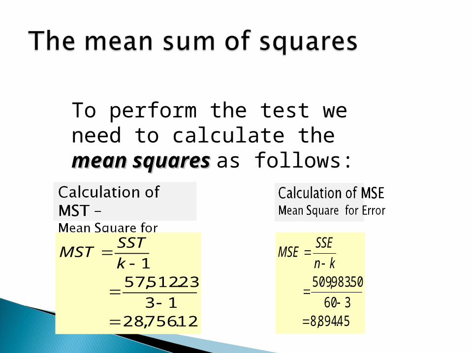
To perform the test we need to calculate the mean mean squaressquares as follows:

12.756,2813

23.512,571

k

SSTMST

45.894,8360

50.983,509

kn

SSEMSE

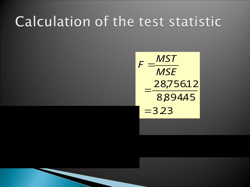
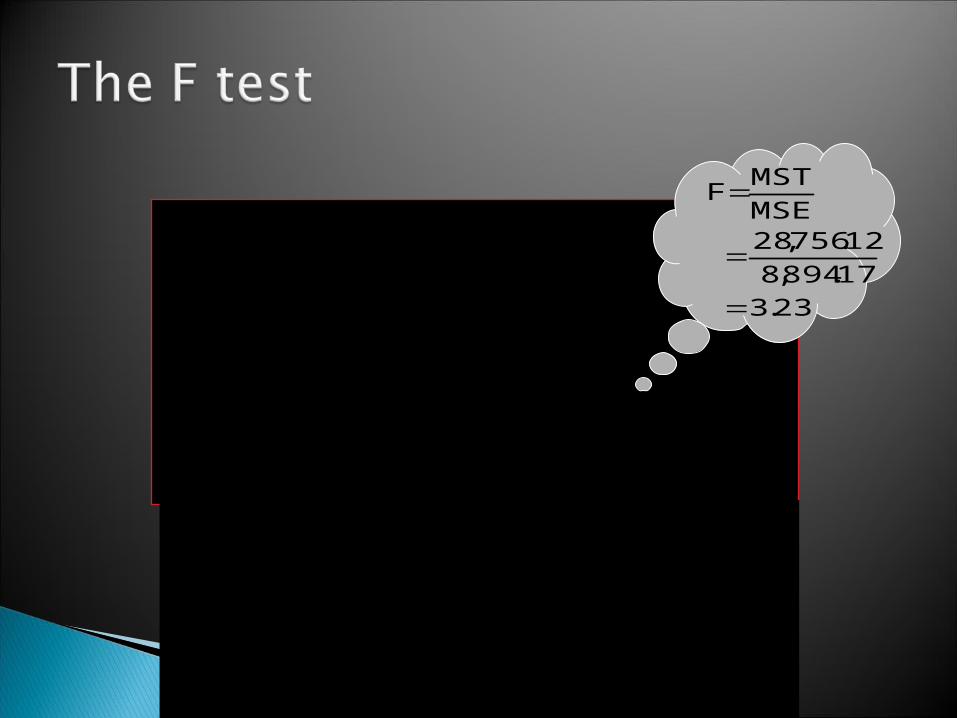
23.3

45.894,8

12.756,28

MSE

MSTF

with the following degrees of freedom:v1=k -1 and v2=n-k

Required Conditions:1. The populations tested are normally distributed.2. The variances of all the populations tested are equal.

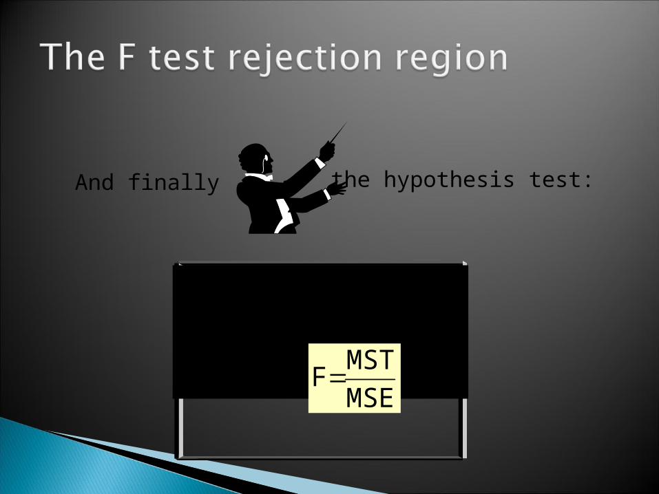
And finally the hypothesis test:

H0: 1 = 2 = …=k

H1: At least two means differ

Test statistic:

R.R: F>F,k-1,n-k MSEMST

F

Ho: 1 = 2= 3

H1: At least two means differ

Test statistic F= MST MSE= 3.23

15.3FFF:.R.R 360,13,05.0knk 1

Since 3.23 > 3.15, there is sufficient evidence to reject Ho in favor of H1, and argue that at least one of the mean sales is different than the others.

23.317.894,812.756,28

MSEMST

F

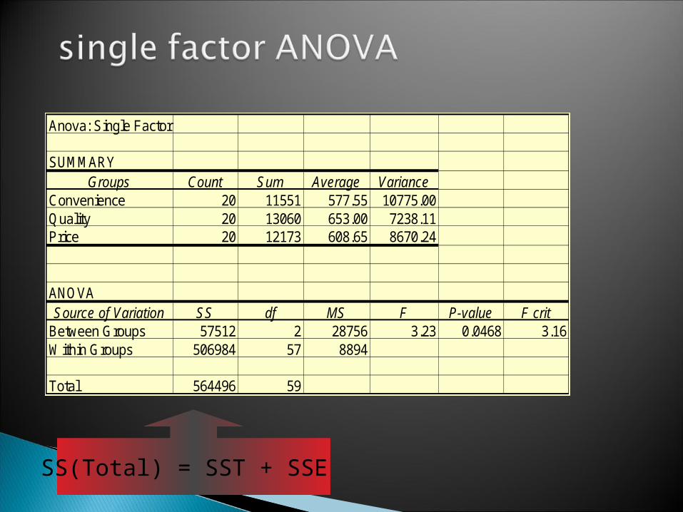
SS(Total) = SST + SSE

Anova: Single Factor

SUMMARYGroups Count Sum Average Variance

Convenience 20 11551 577.55 10775.00Quality 20 13060 653.00 7238.11Price 20 12173 608.65 8670.24

ANOVASource of Variation SS df MS F P-value F crit

Between Groups 57512 2 28756 3.23 0.0468 3.16Within Groups 506984 57 8894

Total 564496 59

Fixed effects◦ If all possible levels of a factor are included in

our analysis we have a fixed effect ANOVA.◦ The conclusion of a fixed effect ANOVA

applies only to the levels studied. Random effects

◦ If the levels included in our analysis represent a random sample of all the possible levels, we have a random-effect ANOVA.

◦ The conclusion of the random-effect ANOVA applies to all the levels (not only those studied).

In some ANOVA models the test statistic of the fixed effects case may differ from the test statistic of the random effect case.

Fixed and random effects - examples◦ Fixed effects - The advertisement Example .All

the levels of the marketing strategies were included

◦ Random effects - To determine if there is a difference in the production rate of 50 machines, four machines are randomly selected and there production recorded.

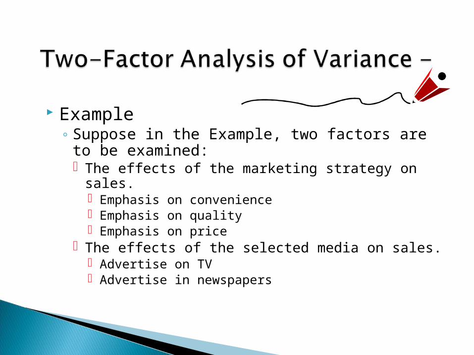
Example◦ Suppose in the Example, two factors are to be

examined: The effects of the marketing strategy on sales.

Emphasis on convenience Emphasis on quality Emphasis on price

The effects of the selected media on sales. Advertise on TV Advertise in newspapers

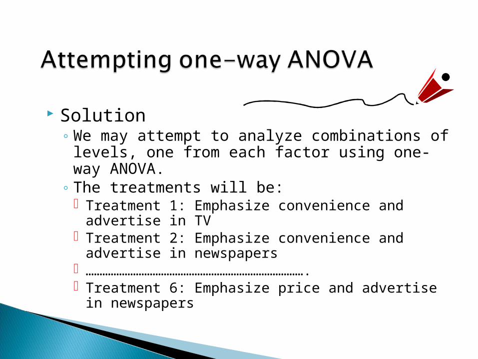
Solution◦ We may attempt to analyze combinations of

levels, one from each factor using one-way ANOVA.

◦ The treatments will be: Treatment 1: Emphasize convenience and advertise

in TV Treatment 2: Emphasize convenience and advertise

in newspapers ……………………………………………………………………. Treatment 6: Emphasize price and advertise in

newspapers

Solution◦The hypotheses tested are:

H0: 1= 2= 3= 4= 5= 6

H1: At least two means differ.

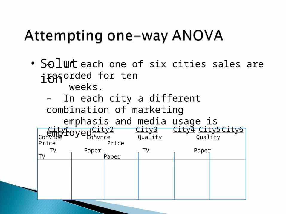
City1 City2 City3 City4 City5 City6Convnce Convnce Quality Quality Price Price

TV Paper TV Paper TV Paper

– In each one of six cities sales are recorded for ten weeks. – In each city a different combination of marketing emphasis and media usage is employed.

• Solution

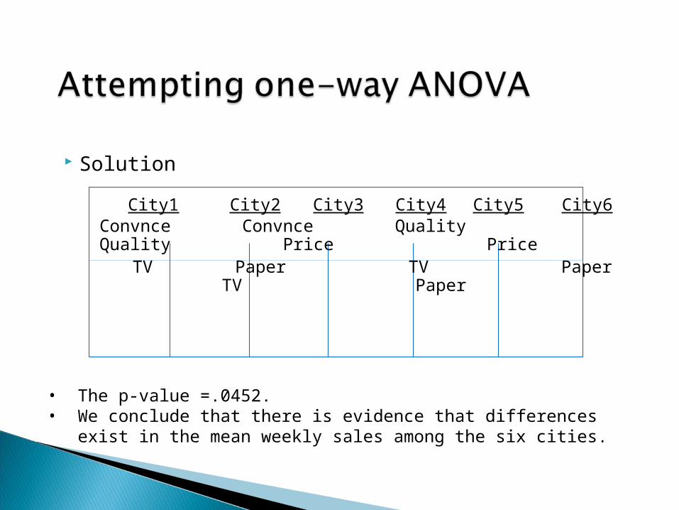
• The p-value =.0452. • We conclude that there is evidence that differences exist in the mean weekly sales among the six cities.

City1 City2 City3 City4 City5 City6Convnce Convnce Quality Quality Price Price

TV Paper TV Paper TV Paper

Solution

These result raises some questions:◦ Are the differences in sales caused by the

different marketing strategies?◦ Are the differences in sales caused by the

different media used for advertising?◦ Are there combinations of marketing strategy

and media that interact to affect the weekly sales?

The current experimental design cannot provide answers to these questions.

A new experimental design is needed.

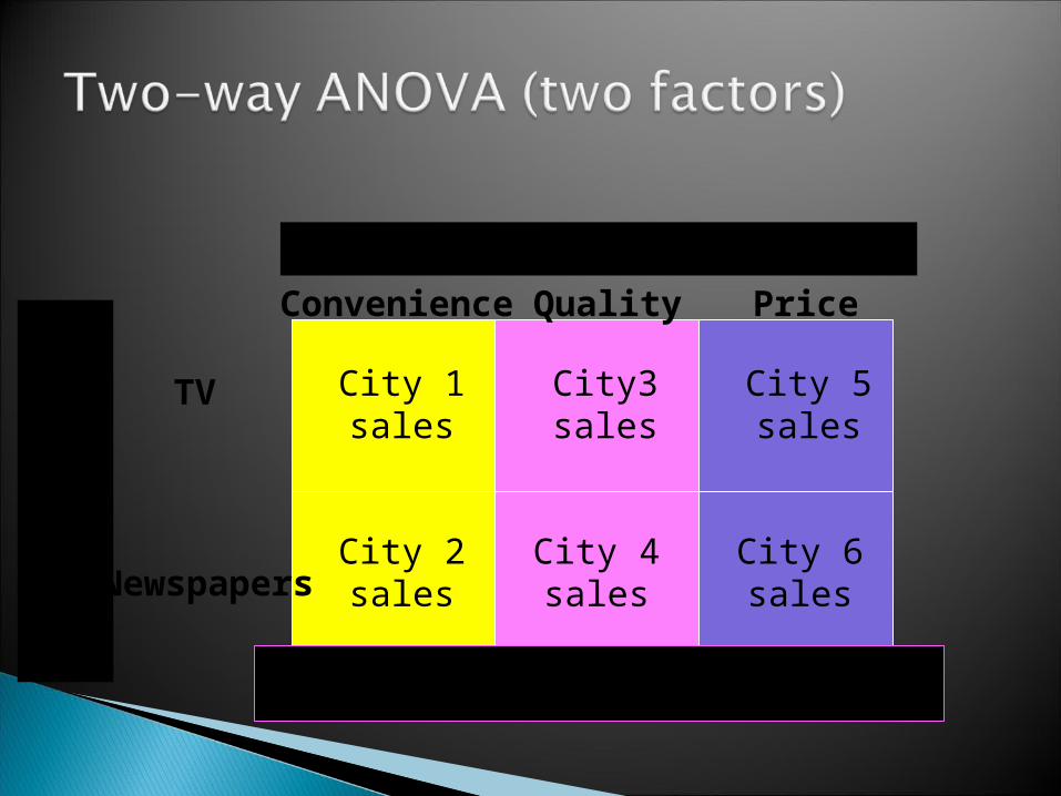
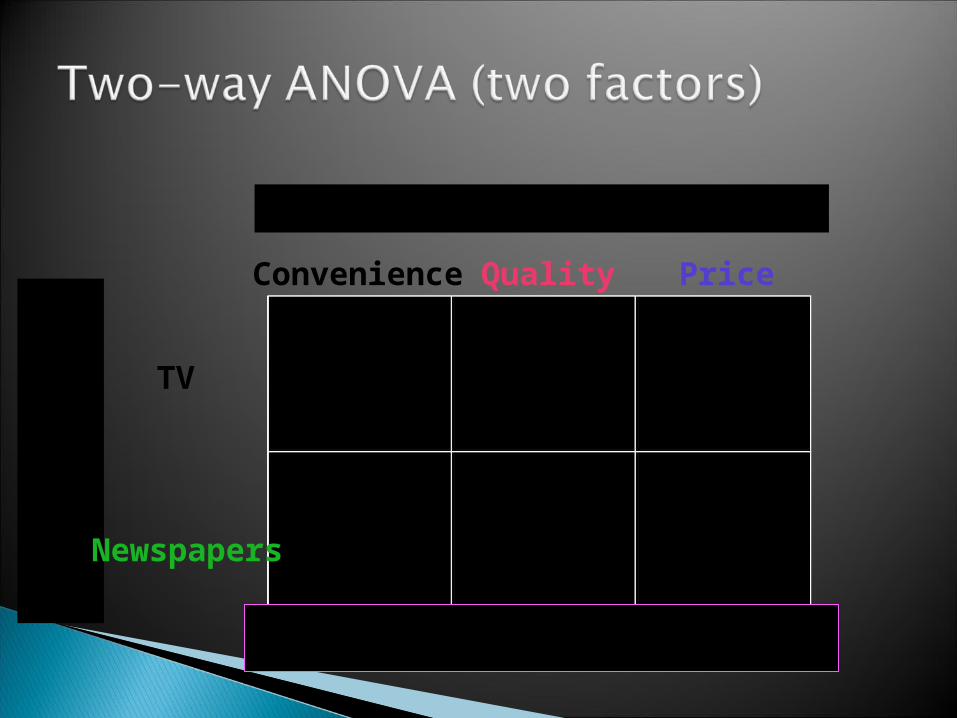
City 1sales

City3sales

City 5sales

City 2sales

City 4sales

City 6sales

TV

Newspapers

Convenience Quality Price

Are there differences in the mean sales caused by different marketing strategies?

Factor A: Marketing strategy

Fact

or

B:

Ad

vert

isin

g m

ed

ia

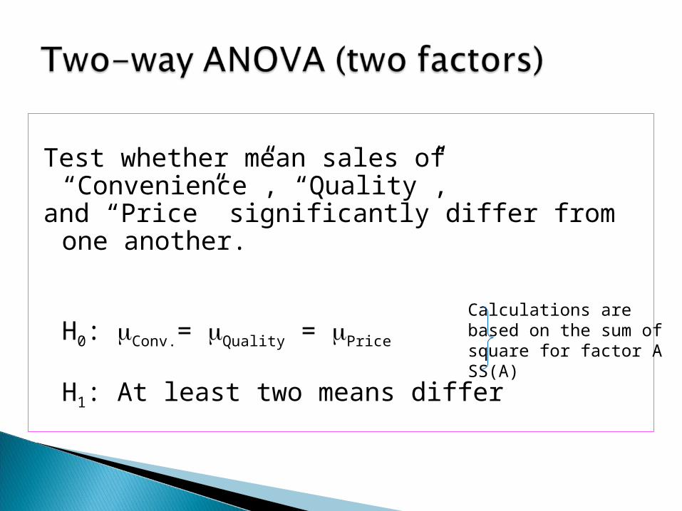
Test whether mean sales of “Convenience”, “Quality”,

and “Price” significantly differ from one another.

H0: Conv.= Quality = Price

H1: At least two means differ

Calculations are based on the sum of square for factor ASS(A)

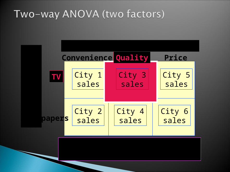
City 1sales

City 3sales

City 5sales

City 2sales

City 4sales

City 6sales

Factor A: Marketing strategy

Fact

or

B:

Ad

vert

isin

g m

ed

ia

Are there differences in the mean sales caused by different advertising media?

TV

Newspapers

Convenience Quality Price

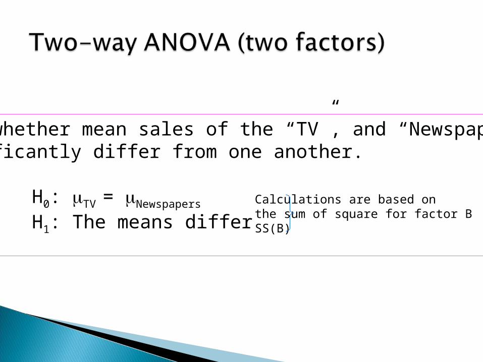
Test whether mean sales of the “TV”, and “Newspapers” significantly differ from one another.

H0: TV = Newspapers

H1: The means differ

Calculations are based onthe sum of square for factor BSS(B)

City 1sales

City 5sales

City 2sales

City 4sales

City 6sales

TV

Newspapers

Convenience Quality Price

Factor A: Marketing strategy

Fact

or

B:

Ad

vert

isin

g m

ed

ia

Are there differences in the mean sales caused by interaction between marketing strategy and advertising medium?

City 3sales

TV

Quality

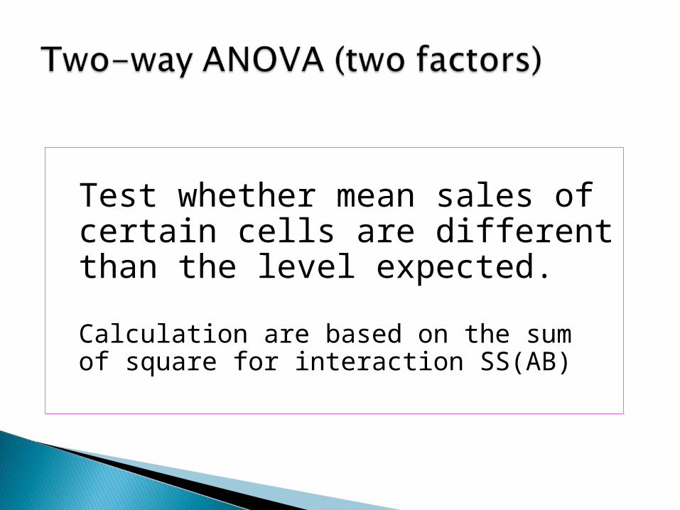
Test whether mean sales of certain cells are different than the level expected.

Calculation are based on the sum of square for interaction SS(AB)

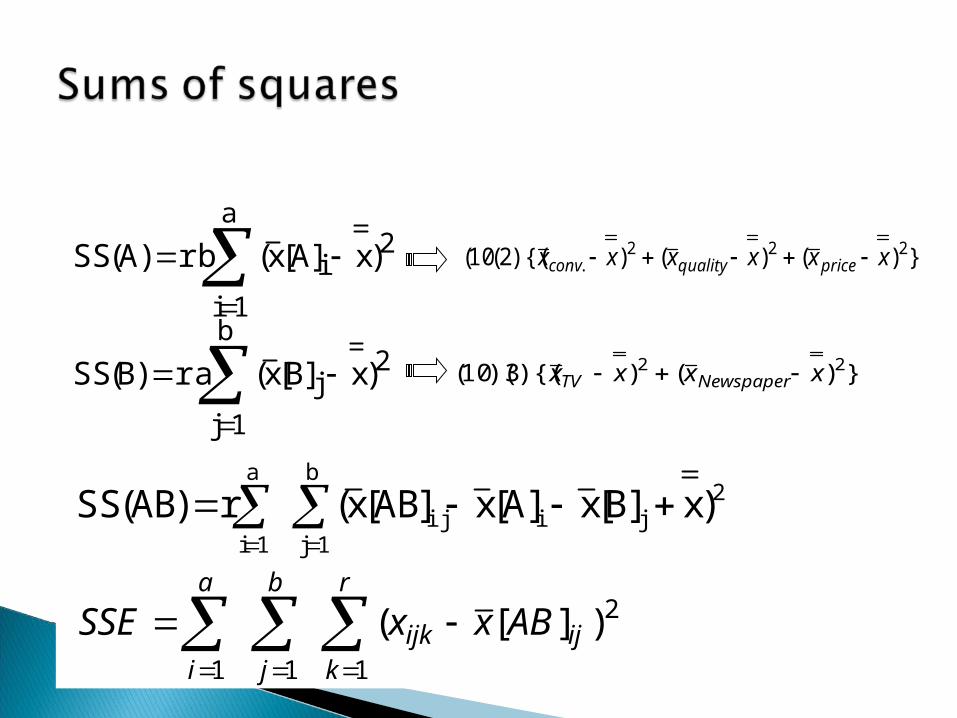
a

1i

2i )x]A[x(rb)A(SS })()()){(2(10( 222

. xxxxxx pricequalityconv

b

1j

2j )x]B[x(ra)B(SS })()){(3)(10( 22 xxxx NewspaperTV

b

1j

2jiij

a

1i

)x]B[x]A[x]AB[x(r)AB(SS

r

kijijk

b

j

a

i

ABxxSSE1

2

11

)][(

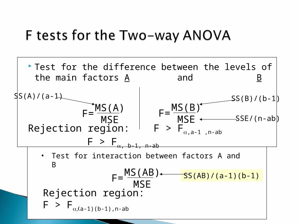
Test for the difference between the levels of the main factors A and B

F= MS(A)MSE

F= MS(B)MSE

Rejection region: F > F,a-1 ,n-ab F > F, b-1, n-ab

• Test for interaction between factors A and B

F= MS(AB)

MSERejection region: F > Fa-1)

(b-1),n-ab

SS(A)/(a-1) SS(B)/(b-1)

SS(AB)/(a-1)(b-1)

SSE/(n-ab)

1. The response distributions is normal2. The treatment variances are equal.3. The samples are independent.

Convenience Quality Price

TV 491 677 575TV 712 627 614TV 558 590 706TV 447 632 484TV 479 683 478TV 624 760 650TV 546 690 583TV 444 548 536TV 582 579 579TV 672 644 795

Newspaper 464 689 803Newspaper 559 650 584Newspaper 759 704 525Newspaper 557 652 498Newspaper 528 576 812Newspaper 670 836 565Newspaper 534 628 708Newspaper 657 798 546Newspaper 557 497 616Newspaper 474 841 587

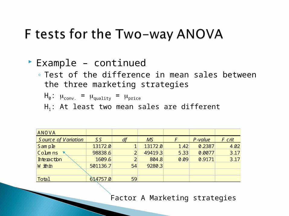
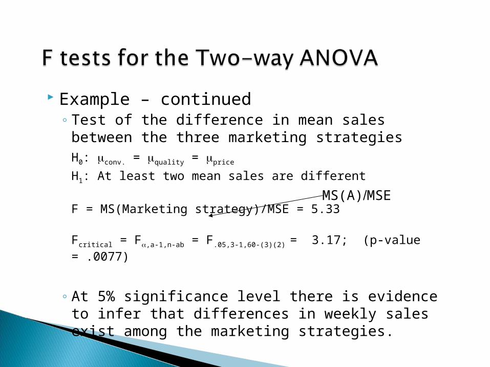
Example – continued◦ Test of the difference in mean sales between the

three marketing strategiesH0: conv. = quality = price

H1: At least two mean sales are different

ANOVASource of Variation SS df MS F P-value F critSample 13172.0 1 13172.0 1.42 0.2387 4.02Columns 98838.6 2 49419.3 5.33 0.0077 3.17Interaction 1609.6 2 804.8 0.09 0.9171 3.17Within 501136.7 54 9280.3

Total 614757.0 59

Factor A Marketing strategies

Example – continued◦ Test of the difference in mean sales between

the three marketing strategiesH0: conv. = quality = price

H1: At least two mean sales are different

F = MS(Marketing strategy)/MSE = 5.33

Fcritical = F,a-1,n-ab = F.05,3-1,60-(3)(2) = 3.17; (p-value = .0077)

◦ At 5% significance level there is evidence to infer that differences in weekly sales exist among the marketing strategies.

MS(A)MSE

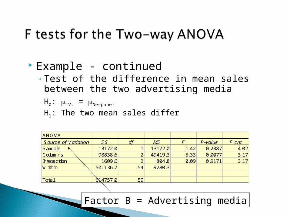
Example - continued◦ Test of the difference in mean sales between

the two advertising mediaH0: TV. = Nespaper

H1: The two mean sales differ

Factor B = Advertising media

ANOVASource of Variation SS df MS F P-value F critSample 13172.0 1 13172.0 1.42 0.2387 4.02Columns 98838.6 2 49419.3 5.33 0.0077 3.17Interaction 1609.6 2 804.8 0.09 0.9171 3.17Within 501136.7 54 9280.3

Total 614757.0 59

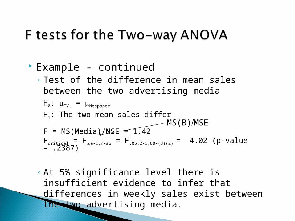
Example - continued◦ Test of the difference in mean sales between

the two advertising mediaH0: TV. = Nespaper

H1: The two mean sales differ

F = MS(Media)/MSE = 1.42 Fcritical = Fa-1,n-ab = F.05,2-1,60-(3)(2) = 4.02 (p-value = .2387)

◦ At 5% significance level there is insufficient evidence to infer that differences in weekly sales exist between the two advertising media.

MS(B)MSE

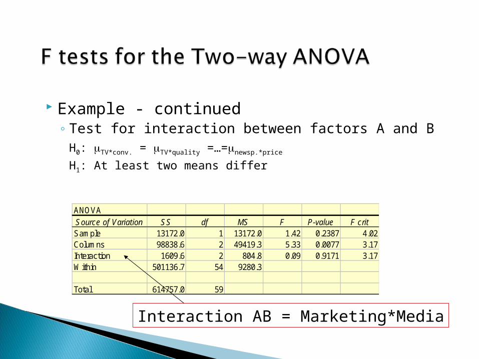
Example - continued◦ Test for interaction between factors A and B

H0: TV*conv. = TV*quality =…=newsp.*price

H1: At least two means differ

Interaction AB = Marketing*Media

ANOVASource of Variation SS df MS F P-value F critSample 13172.0 1 13172.0 1.42 0.2387 4.02Columns 98838.6 2 49419.3 5.33 0.0077 3.17Interaction 1609.6 2 804.8 0.09 0.9171 3.17Within 501136.7 54 9280.3

Total 614757.0 59

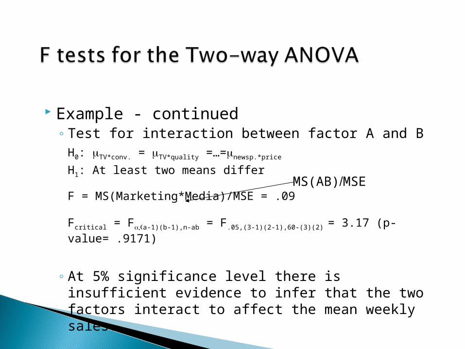
Example - continued◦ Test for interaction between factor A and B

H0: TV*conv. = TV*quality =…=newsp.*price

H1: At least two means differ

F = MS(Marketing*Media)/MSE = .09

Fcritical = Fa-1)(b-1),n-ab = F.05,(3-1)(2-1),60-(3)(2) = 3.17 (p-value= .9171)

◦ At 5% significance level there is insufficient evidence to infer that the two factors interact to affect the mean weekly sales.

MS(AB)MSE

• To compare 2 or more means in a single test we use ANOVA

• The type of ANOVA test to use is decided by the number of FACTORS in the experiment

• The ANOVA will only tell whether there is a significant difference and gives no information on which mean(s) are different

• Further pairwise comparisons of the means are required to gain

further information on which mean(s) are different

• Pairwise testing of means can increase the probability of type 1 errors

If we have to go do pair wise t-tests after the ANOVA anyway,

why not just do them and forget the ANOVA? – Well of course that is their choice BUT the ANOVA may return a result of no sig diff. In one test, saving a lot of time and effort AND pairwise testing increases the probability of false results

Thank You