Embed Size (px)
Citation preview
7/27/2019 SisteMatic Review PsMt Ho Emmes
http://slidepdf.com/reader/full/sistematic-review-psmt-ho-emmes 1/31
This article was downloaded by: [FU Berlin]On: 28 July 2013, At: 16:17Publisher: RoutledgeInforma Ltd Registered in England and Wales Registered Number: 1072954Registered office: Mortimer House, 37-41 Mortimer Street, London W1T 3JH,UK
Multivariate Behavioral
ResearchPublication details, including instructions for
authors and subscription information:
http://www.tandfonline.com/loi/hmbr20
A Systematic Review of
Propensity Score Methods in
the Social SciencesFelix J. Thoemmes
a& Eun Sook Kim
b
aUniversity of Tübingen
bTexas A&M University
Published online: 18 Feb 2011.
To cite this article: Felix J. Thoemmes & Eun Sook Kim (2011) A Systematic Review
of Propensity Score Methods in the Social Sciences, Multivariate Behavioral Research,
46:1, 90-118, DOI: 10.1080/00273171.2011.540475
To link to this article: http://dx.doi.org/10.1080/00273171.2011.540475
PLEASE SCROLL DOWN FOR ARTICLE
Taylor & Francis makes every effort to ensure the accuracy of all theinformation (the “Content”) contained in the publications on our platform.However, Taylor & Francis, our agents, and our licensors make norepresentations or warranties whatsoever as to the accuracy, completeness,or suitability for any purpose of the Content. Any opinions and viewsexpressed in this publication are the opinions and views of the authors, andare not the views of or endorsed by Taylor & Francis. The accuracy of the
Content should not be relied upon and should be independently verified withprimary sources of information. Taylor and Francis shall not be liable for anylosses, actions, claims, proceedings, demands, costs, expenses, damages,and other liabilities whatsoever or howsoever caused arising directly orindirectly in connection with, in relation to or arising out of the use of theContent.

7/27/2019 SisteMatic Review PsMt Ho Emmes
http://slidepdf.com/reader/full/sistematic-review-psmt-ho-emmes 2/31
This article may be used for research, teaching, and private study purposes.Any substantial or systematic reproduction, redistribution, reselling, loan,sub-licensing, systematic supply, or distribution in any form to anyone isexpressly forbidden. Terms & Conditions of access and use can be found athttp://www.tandfonline.com/page/terms-and-conditions
D o w n l o a d e d b y [ F U B
e r l i
n ] a t 1 6 : 1 7 2 8 J u l y 2 0 1 3
7/27/2019 SisteMatic Review PsMt Ho Emmes
http://slidepdf.com/reader/full/sistematic-review-psmt-ho-emmes 3/31
Multivariate Behavioral Research, 46:90–118, 2011
Copyright © Taylor & Francis Group, LLC
ISSN: 0027-3171 print/1532-7906 online
DOI: 10.1080/00273171.2011.540475
A Systematic Review of PropensityScore Methods in the Social Sciences
Felix J. Thoemmes
University of Tübingen
Eun Sook Kim
Texas A&M University
The use of propensity scores in psychological and educational research has been
steadily increasing in the last 2 to 3 years. However, there are some common
misconceptions about the use of different estimation techniques and condition-
ing choices in the context of propensity score analysis. In addition, reportingpractices for propensity score analyses often lack important details that allow
other researchers to confidently judge the appropriateness of reported analyses and
potentially to replicate published findings. In this article we conduct a systematic
literature review of a large number of published articles in major areas of social
science that used propensity scores up until the fall of 2009. We identify common
errors in estimation, conditioning, and reporting of propensity score analyses and
suggest possible solutions.
Propensity score methods, as originally proposed by Rosenbaum and Rubin(1983), are experiencing a tremendous increase of interest in many scientific
areas including the social sciences. The number of newly published articles each
year that used propensity scores in the psychological and educational literature,
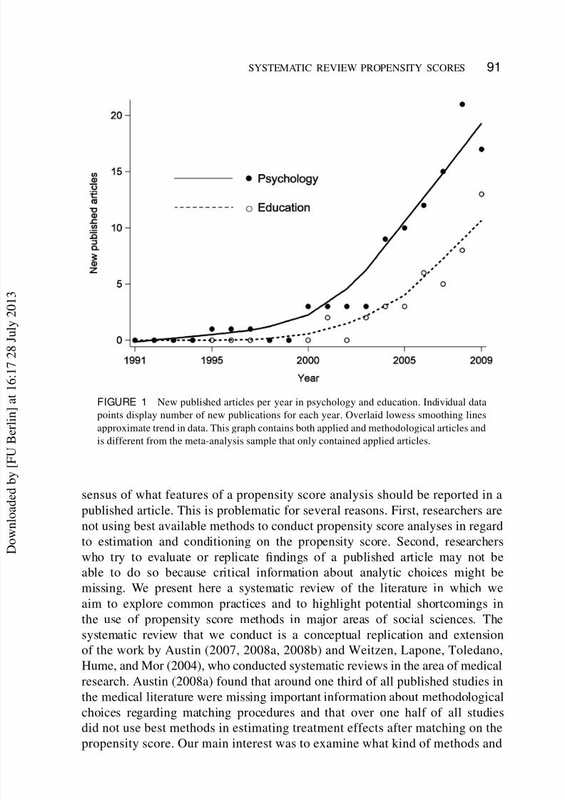
as assessed by the database Web of Science, is rising nearly exponentially (see
Figure 1). This development clearly demonstrates that there is interest in this
methodological tool.
However, there exists much variability on how propensity score methods
are implemented in practice and recent methodological advances are not fully
incorporated in the substantive literature yet. In addition, there is lack of con-
Correspondence concerning this article should be addressed to Felix J. Thoemmes, University
of Tübingen, Europastr. 6, 72072 Tübingen, Germany. E-mail: [email protected]
90
D o w n l o a d e d b y [ F U B
e r l i
n ] a t 1 6 : 1 7 2 8 J u l y 2 0 1 3
7/27/2019 SisteMatic Review PsMt Ho Emmes
http://slidepdf.com/reader/full/sistematic-review-psmt-ho-emmes 4/31
SYSTEMATIC REVIEW PROPENSITY SCORES 91
FIGURE 1 New published articles per year in psychology and education. Individual data
points display number of new publications for each year. Overlaid lowess smoothing lines
approximate trend in data. This graph contains both applied and methodological articles and
is different from the meta-analysis sample that only contained applied articles.
sensus of what features of a propensity score analysis should be reported in a
published article. This is problematic for several reasons. First, researchers are
not using best available methods to conduct propensity score analyses in regard
to estimation and conditioning on the propensity score. Second, researchers
who try to evaluate or replicate findings of a published article may not beable to do so because critical information about analytic choices might be
missing. We present here a systematic review of the literature in which we
aim to explore common practices and to highlight potential shortcomings in
the use of propensity score methods in major areas of social sciences. The
systematic review that we conduct is a conceptual replication and extension
of the work by Austin (2007, 2008a, 2008b) and Weitzen, Lapone, Toledano,
Hume, and Mor (2004), who conducted systematic reviews in the area of medical
research. Austin (2008a) found that around one third of all published studies in
the medical literature were missing important information about methodologicalchoices regarding matching procedures and that over one half of all studies
did not use best methods in estimating treatment effects after matching on the
propensity score. Our main interest was to examine what kind of methods and
D o w n l o a d e d b y [ F U B
e r l i
n ] a t 1 6 : 1 7 2 8 J u l y 2 0 1 3
7/27/2019 SisteMatic Review PsMt Ho Emmes
http://slidepdf.com/reader/full/sistematic-review-psmt-ho-emmes 5/31
92 THOEMMES AND KIM
reporting patterns in regard to propensity score analyses were most prevalent
in the social science literature, specifically in psychological and educational
research. Before presentation of our methods and results we provide a brief overview of necessary steps in a propensity score analysis. For more detailed
overviews we refer the reader to introductions and applied examples by Caliendo
& Kopeinig (2008), Stuart (2010), Stuart et al. (2009), or Shadish and Steiner
(2010). A more thorough treatment involving general issues of the design and
analysis of observational studies is given by Rosenbaum (2010).
WHAT IS THE PROPENSITY SCORE?
Briefly explained, the propensity score is a conditional probability that expresses
how likely a participant is to be assigned or to select the treatment condition
given certain observed baseline characteristics. In a propensity score analysis this
conditional probability is used to condition observed data, for example, through
matching or stratification on the propensity score. The aim of conditioning on
the propensity score is to achieve balance on the observed covariates and recreate
a situation that would have been expected in a randomized experiment. Balance
on covariates is desirable because a balanced covariate (which is by definition
uncorrelated with treatment assignment) cannot bias the estimate of a treatmenteffect, even if the covariate itself is related to an outcome variable. An important
insight from Rosenbaum and Rubin (1983) was that balance on the propensity
score produces on average balance on observed covariates. Under the assumption
that all relevant covariates have been assessed, a propensity score analysis can
yield unbiased causal effect estimates. More formally, the key assumption of
a viable propensity score analysis is the so-called strongly ignorable treatment
assignment assumption. This assumption holds if the potential outcomes Y 0 and
Y 1 are conditionally independent of treatment assignment Z, given a vector
of covariates X .1
The potential outcomes are unobserved quantities that referto potentially observable values if a particular unit were assigned to either
treatment or control condition. For more information on potential outcomes
and the strongly ignorable treatment assignment assumption see Rosenbaum
and Rubin (1983) or Rubin (2005).
It should be noted that this assumption cannot be empirically tested—
researchers can only attempt to build a convincing case that all important
covariates have been assessed or employ actual randomization of treatment
assignment, which ensures that all observed and unobserved covariates are on
1Another part of this assumption is that no propensity scores with the two extreme values of 0
and 1 are observed, or in other words each unit has a nonzero probability of being either assigned
to the treatment or the control condition.
D o w n l o a d e d b y [ F U B
e r l i
n ] a t 1 6 : 1 7 2 8 J u l y 2 0 1 3
7/27/2019 SisteMatic Review PsMt Ho Emmes
http://slidepdf.com/reader/full/sistematic-review-psmt-ho-emmes 6/31
SYSTEMATIC REVIEW PROPENSITY SCORES 93
average balanced prior to treatment administration. Sensitivity analyses (e.g.,
Robins, Rotnitzky, & Scharfstein, 1999; Rosenbaum, 1991a, 1991b) that probe
how much bias an unobserved covariate would have to exert to negate theobserved treatment effect can help to bolster one’s faith in the assumption that
all important covariates and potential confounders have been assessed.
To put the propensity score technique into an applied context, consider an
example in which an estimate of the effect of retaining young schoolchildren
on later academic achievement is of interest (e.g., Hong & Raudenbush, 2005;
Hughes, Chen, Thoemmes, & Kwok, 2010; Wu, West, & Hughes, 2008). Be-
cause retention of schoolchildren is not randomized, an unadjusted estimate
of the treatment effect of the retention policy could be potentially biased.
Children who are retained differ on many characteristics, such as intelligence oracademic performance prior to retention. In fact, one would assume that the least
academically gifted children would be retained and more academically gifted
children promoted. Comparing academic achievement between retained and
promoted children at a later point in time would yield a biased treatment effect of
retention because children in the retained and promoted group were so dissimilar
at the onset of the study. Using propensity score analysis can potentially mitigate
these biases. In particular, researchers can estimate propensity scores based on
important student characteristics and assign probabilities of retention based on
an extensive list of covariates to each single child. In a next step, childrenwith similar propensity scores (and therefore similar conditional probability of
being retained) but different retention or promotion status can be matched on
the propensity score. The assumption is that the matched samples of children
are identical (or at least comparable) on many background characteristics and
only differ in their retention status—just as we would expect from a randomized
experiment. Differences between the groups of retained and promoted children
in the matched sample can then be assessed and interpreted.
USE OF THE PROPENSITY SCORE
In this section we briefly illustrate how the propensity score is used and which
analytic choices are being made on the part of the researcher. Although this
section is not meant to be a formal introduction to the use of propensity
scores (which can be found elsewhere; e.g., Stuart, 2010), it should serve the
purpose of demonstrating that researchers can use different analytic approaches
when performing a propensity score analysis. Because of this methodological
variability associated with propensity score analyses, it is important that choicesmade in the process are explicated in published work.
A propensity score analysis can only be as good as the covariates that are
at the disposal of the researcher. Only a rich set of covariates can make the
D o w n l o a d e d b y [ F U B
e r l i
n ] a t 1 6 : 1 7 2 8 J u l y 2 0 1 3
7/27/2019 SisteMatic Review PsMt Ho Emmes
http://slidepdf.com/reader/full/sistematic-review-psmt-ho-emmes 7/31
94 THOEMMES AND KIM
strongly ignorable treatment assignment assumption credible and therefore it is
of importance that researchers give a detailed account of the variables that were
collected. Other researchers depend on that information to judge the quality of the analysis. It is usually not sufficient to just use demographic data such as age,
gender, and ethnicity. Propensity score models that are conducted with only few
covariates often do not yield unbiased causal effect estimates (Shadish, Luellen,
& Clark, 2006).
After many covariates have been collected, the propensity score is estimated.
Theoretically any model that produces estimates of the probability of group
membership for each participant can be used to estimate propensity scores.
Examples are logistic regression, probit regression, or discriminant analysis.
More recent work has employed methods based on data mining algorithms (e.g.,boosted regression trees; McCaffrey, Ridgeway, & Morral, 2004). However, these
techniques are not widely used yet.
It is, however, insufficient to simply report the type of model that was used
for estimation. More detail is needed as to how variables were included or ex-
cluded in the model. Common choices for model selection are nonparsimonious
models (in which all variables are included) or approaches based on statistical
significance, often with significance levels that are larger than the usual .05
cutoff (see, e.g., Shadish et al., 2006). No definite answer exists as to which
cutoff value will produce the best balance and it is unclear if one single optimalcutoff value would work for a range of different data sets.
After estimation of the propensity score the data is conditioned, for example,
using matching (e.g., Rubin & Thomas, 1992, 1996), adjustment by subclas-
sification or stratification (e.g., Lunceford & Davidian, 2004; Myers & Louis,
2007; Rosenbaum & Rubin, 1984), or weighting (e.g., Hirano & Imbens, 2001).
Another approach that is occasionally encountered in applied research (see,
e.g., Weitzen et al., 2004, for an overview) is to use the propensity score as
a covariate in an Analysis of Covariance (ANCOVA) type model. However,
this approach is not recommended because it has additional assumptions uniqueto regression adjustment, namely, that the relationship between the estimated
propensity score and the outcome must be linear and that no propensity score
by treatment interaction exists.
Each of these approaches will in most circumstances result in slightly different
estimates and it is therefore necessary to report on the details of the particu-
lar method that was chosen. Especially matching, even though conceptually
straightforward, can be implemented operationally using several different and
complex procedures. Without going into detail on the subtleties of matching, we
briefly mention that widely varying methods exist and therefore reporting of howmatching was performed is important. Broadly speaking, matching strategies
can be distinguished by several different factors. One distinguishing factor is
how many treated units are being matched to control units and vice versa. In
D o w n l o a d e d b y [ F U B
e r l i
n ] a t 1 6 : 1 7 2 8 J u l y 2 0 1 3
7/27/2019 SisteMatic Review PsMt Ho Emmes
http://slidepdf.com/reader/full/sistematic-review-psmt-ho-emmes 8/31
SYSTEMATIC REVIEW PROPENSITY SCORES 95
the simplest case, the units are matched 1:1, which means that one unit in the
treatment group is matched to one unit in the control group. A related approach to
retain additional units is to match several control units to a single treated unit, so-called one-to-many matching. This can be achieved by matching each participant
to a fixed number of participants in the other group (e.g., one-to-three matching)
or to a variable number of participants, depending on the availability of adequate
matches. Ming and Rosenbaum (2000, 2001) describe algorithms to perform
one-to-many matching. A special case of one-to-many matching is full matching
(Hansen, 2004; Rosenbaum, 1991c) in which many control units are matched
to one treated unit and many treated units are matched to a single control unit.
Another dimension on which matching algorithms can be differentiated is
whether exact or approximate matching is employed. Exact matching requirestwo units to be identical on the propensity score. An alternative is to match
units that have approximately the same propensity score, often called “nearest
neighbor” matching. In this approach a unit is matched to another unit that is
closest to it in terms of the estimated propensity score. To avoid bad matches
that have very different propensity scores, a “caliper” can be defined. A caliper is
a predetermined maximum discrepancy for each matched pair on the propensity
score for which matches are allowed. When using caliper methods, researchers
should report the width of this caliper (e.g., Rosenbaum & Rubin, 1985, suggest
that the caliper width should be set to one quarter of a standard deviation of the logit of the propensity score). A related strategy is to introduce penalties to
distance scores between two participants if their distance to each other exceeds
a certain threshold (Haviland, Nagin, & Rosenbaum, 2007).
A third dimension to distinguish matching schemes is whether matches are
formed to minimize the average absolute distance on the propensity score of
all units in the whole matched sample (“optimal matching”; Gu & Rosenbaum,
1993; Hansen, 2004; Rosenbaum, 1989) or whether a single match is formed
with the best available unit one at a time without trying to minimize average
distance globally (“greedy matching”). It should be noted that still other match-ing algorithms exist (e.g., kernel matching; Heckman, Ichimura, & Todd, 1997,
1998), which we do not discuss here due to their infrequent use in the social
sciences.
If conditioning methods other than matching are used, it is also important
to report accompanying details. For example, if participants are stratified based
on the propensity score, it is necessary to report how the strata were formed
and also how many strata were formed. A common choice is to subclassify data
into at least five strata defined by the propensity score as studies by Cochran
(1968) have shown that five strata remove approximately 90% of the bias dueto measured confounders when estimating a linear treatment effect. The strata
are usually chosen to be of equal size but can also be chosen to minimize the
variance of the treatment effect estimate (Hullsiek & Louis, 2002).
D o w n l o a d e d b y [ F U B
e r l i
n ] a t 1 6 : 1 7 2 8 J u l y 2 0 1 3
7/27/2019 SisteMatic Review PsMt Ho Emmes
http://slidepdf.com/reader/full/sistematic-review-psmt-ho-emmes 9/31
96 THOEMMES AND KIM
Finally, it is possible to use the propensity score as a weight in an analysis.
Several authors describe this approach (e.g., Hirano, Imbens, & Ridder, 2003;
Lunceford & Davidian, 2004; McCaffrey et al., 2004). Usually a weightingscheme is employed in which each treated observation is weighted by the inverse
of the propensity score; each unit in the control group is weighted by the inverse
of 1 minus the propensity score. Kang and Schafer (2007) and Schafer and Kang
(2008) report that weighting estimates have the disadvantage that they can be
highly influenced by weights that are assigned to participants whose propensity
scores are very close to the boundary values of 0 or 1. Furthermore, weighting
estimates are associated with computation of so-called robust (“sandwich”)
estimators for model standard errors.
An important part of the propensity score analysis is a careful check of modeladequacy and underlying assumptions. Two central properties of the propensity
score model should always be assessed and reported: the balance property and
the common support region. The balance property describes whether balance
in terms of means and variances has been achieved on the covariates (and
potentially on interactions and polynomial terms). The common support region,
on the other hand, describes the region of overlap between the two propensity
score distributions. A broad region of common support allows causal effect
estimates over the full range of propensity scores in the sample, whereas small
common support regions restrict the estimation of a causal effect to a subsamplewithin a specified region of a propensity score distribution.
Different methods exist to check both of these properties. A straightforward
method to check balance involves testing covariates (and potentially interactions
and polynomial terms; e.g., Austin, 2009a; Rubin & Waterman, 2006) for signif-
icant differences between the treated and control group in the matched sample
(e.g., Hansen, 2004, 2008; Rosenbaum & Rubin, 1983). Absence of significant
differences is taken as evidence that balance has been achieved. Other authors
(e.g., Austin, 2007; Ho, Imai, King, & Stuart, 2007) criticize significance tests
in the context of matching due to the dependence on sample size and suggestexamining standardized differences before and after matching. This standardized
difference is well known to psychologists as Cohen’s d (Cohen, 1988). A caveat,
as noted by, for example, Stuart (2008) is that the same denominator term (i.e.,
the same standard deviation) across unmatched and matched sample should be
used to determine the standardized difference.
Balance of the propensity score or the covariates themselves can also be
examined graphically (e.g., see Helmreich & Pruzek, 2009). Different graphical
methods can be used, for example, comparing box plots (Tukey, 1977) for
each covariate in the two groups, plotting and comparing histograms or kerneldensity estimates of the distributions in each group, or using Q-Q plots of
the propensity scores or covariates in both groups. Austin (2009a) notes that
graphical approaches, in particular the comparisons of the distribution of the
D o w n l o a d e d b y [ F U B
e r l i
n ] a t 1 6 : 1 7 2 8 J u l y 2 0 1 3
7/27/2019 SisteMatic Review PsMt Ho Emmes
http://slidepdf.com/reader/full/sistematic-review-psmt-ho-emmes 10/31
SYSTEMATIC REVIEW PROPENSITY SCORES 97
propensity score, are often not helpful in evaluating differences on covari-
ates.
Another step in assessing model adequacy is to determine whether the propen-sity distributions of the two groups have sufficient overlap. This is usually done
by examining the range of the propensity score distributions in the treatment
and control group. The common support region is especially important because
it is intimately linked to the type of generalization of the causal effect that is
possible from the analysis. Generally speaking, it is advisable to exclude units
that fall outside the common support region as no causal effect is defined for
these units. Imai, King, and Stuart (2008) and King and Zeng (2007) provide
an overview of this issue.
The last step in the propensity score analysis is the actual estimation of thetreatment effect corrected for potential bias. The choice of the treatment effect
estimation model depends partly on the conditioning scheme that was chosen
earlier. Currently an issue of debate is whether statistical procedures following
matching on the propensity score need to be adjusted for the matched nature
of the sample. Schafer and Kang (2008) remark in the context of propensity
score matching that “there is no reason to believe that the outcomes of matched
individuals are correlated in any way” (p. 41) and that therefore the use of the
independent sample standard errors is justified, a point that is echoed by Stuart
(2008). Austin (2008a), on the other hand, urges researchers to use standarderrors that account for matched samples, such as the dependent samples t test
standard error. Austin (2009b) also conducted simulation studies showing that
analyses that accounted for the matched nature of the data had Type I error rates
and confidence intervals closer to the nominal levels. Hill (2008) argues that the
exact nature of how this adjustment for matched data should be conducted is
still open to debate.
The preceding section illustrated that a propensity score analysis can be
implemented with many varying methodological choices that have to be made
at every stage of the procedure. We attempt in this systematic literature reviewto provide an overview about the methods that are actually being used by
researchers in the social science and hope to comment on areas that could
potentially be improved.
METHODS
To determine the sample for our systematic literature review we searched three
major social science databases (Web of Science, ERIC, and PsycINFO). We usedthe search term propensity score throughout all searches and did not impose
any limits on other search criteria, for example, year published or type of
publication. There was substantial overlap of the published papers found in
D o w n l o a d e d b y [ F U B
e r l i
n ] a t 1 6 : 1 7 2 8 J u l y 2 0 1 3
7/27/2019 SisteMatic Review PsMt Ho Emmes
http://slidepdf.com/reader/full/sistematic-review-psmt-ho-emmes 11/31
98 THOEMMES AND KIM
all three databases. We refined the results from Web of Science by including
only studies that were published in the areas of psychology, education, and
other social sciences. Studies published in other areas, for example, medicine,economics, health care, and so on, were excluded. This search procedure yielded
a total of 111 published articles. After an additional refining (e.g., excluding
purely methodological papers or articles that used the term propensity score
outside its statistical meaning), 86 relevant papers were selected for the final
analysis sample of the systematic literature review. All included papers are
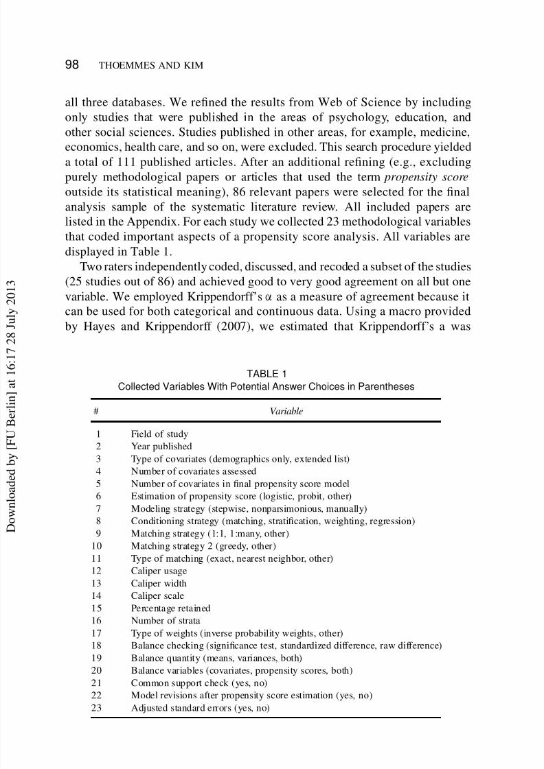
listed in the Appendix. For each study we collected 23 methodological variables
that coded important aspects of a propensity score analysis. All variables are
displayed in Table 1.
Two raters independently coded, discussed, and recoded a subset of the studies(25 studies out of 86) and achieved good to very good agreement on all but one
variable. We employed Krippendorff’s ’ as a measure of agreement because it
can be used for both categorical and continuous data. Using a macro provided
by Hayes and Krippendorff (2007), we estimated that Krippendorff’s a was
TABLE 1
Collected Variables With Potential Answer Choices in Parentheses
# Variable
1 Field of study
2 Year published
3 Type of covariates (demographics only, extended list)
4 Number of covariates assessed
5 Number of covariates in final propensity score model
6 Estimation of propensity score (logistic, probit, other)
7 Modeling strategy (stepwise, nonparsimonious, manually)
8 Conditioning strategy (matching, stratification, weighting, regression)
9 Matching strategy (1:1, 1:many, other)
10 Matching strategy 2 (greedy, other)
11 Type of matching (exact, nearest neighbor, other)
12 Caliper usage
13 Caliper width
14 Caliper scale
15 Percentage retained
16 Number of strata
17 Type of weights (inverse probability weights, other)
18 Balance checking (significance test, standardized difference, raw difference)
19 Balance quantity (means, variances, both)
20 Balance variables (covariates, propensity scores, both)21 Common support check (yes, no)
22 Model revisions after propensity score estimation (yes, no)
23 Adjusted standard errors (yes, no)
D o w n l o a d e d b y [ F U B
e r l i
n ] a t 1 6 : 1 7 2 8 J u l y 2 0 1 3
7/27/2019 SisteMatic Review PsMt Ho Emmes
http://slidepdf.com/reader/full/sistematic-review-psmt-ho-emmes 12/31
SYSTEMATIC REVIEW PROPENSITY SCORES 99
above the minimally acceptable threshold of .667 (Krippendorff, 2004) for all
but one variable. For most variables a was close to .80. The variable for which
we failed to achieve acceptable reliability .’D
:14/ was the percentage of units that were retained after matching. We do not interpret the actual value
of this variable but discuss implications and causes of the low reliability. The
remaining portions of studies were divided between the two coders and coded
individually.
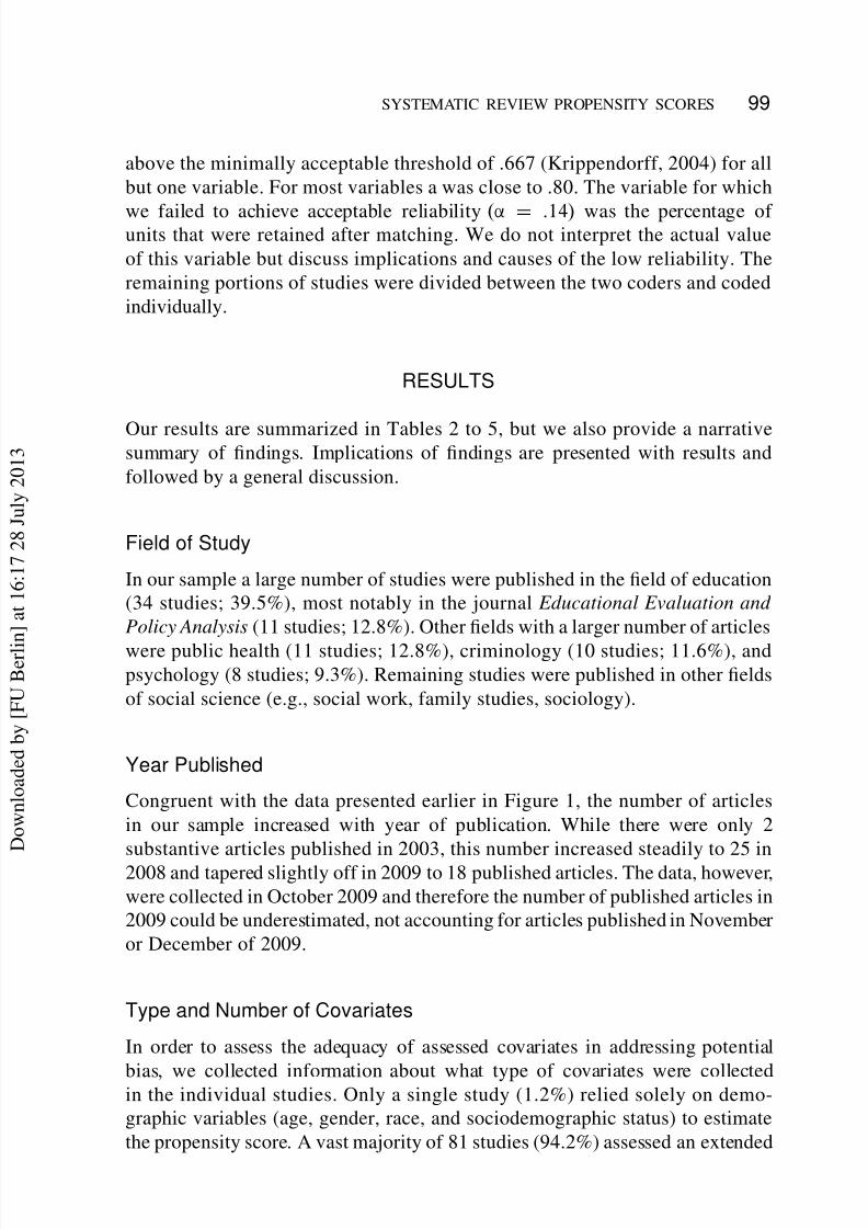
RESULTS
Our results are summarized in Tables 2 to 5, but we also provide a narrativesummary of findings. Implications of findings are presented with results and
followed by a general discussion.
Field of Study
In our sample a large number of studies were published in the field of education
(34 studies; 39.5%), most notably in the journal Educational Evaluation and
Policy Analysis (11 studies; 12.8%). Other fields with a larger number of articles
were public health (11 studies; 12.8%), criminology (10 studies; 11.6%), andpsychology (8 studies; 9.3%). Remaining studies were published in other fields
of social science (e.g., social work, family studies, sociology).
Year Published
Congruent with the data presented earlier in Figure 1, the number of articles
in our sample increased with year of publication. While there were only 2
substantive articles published in 2003, this number increased steadily to 25 in
2008 and tapered slightly off in 2009 to 18 published articles. The data, however,
were collected in October 2009 and therefore the number of published articles in
2009 could be underestimated, not accounting for articles published in November
or December of 2009.
Type and Number of Covariates
In order to assess the adequacy of assessed covariates in addressing potential
bias, we collected information about what type of covariates were collectedin the individual studies. Only a single study (1.2%) relied solely on demo-
graphic variables (age, gender, race, and sociodemographic status) to estimate
the propensity score. A vast majority of 81 studies (94.2%) assessed an extended
D o w n l o a d e d b y [ F U B
e r l i
n ] a t 1 6 : 1 7 2 8 J u l y 2 0 1 3
7/27/2019 SisteMatic Review PsMt Ho Emmes
http://slidepdf.com/reader/full/sistematic-review-psmt-ho-emmes 13/31
100 THOEMMES AND KIM
TABLE 2
Raw Frequencies and Percentages of Categorical Variables
for the Complete Sample of 86 Studies
Variable Count Frequencies (%)
Type of covariates
Extended list 81 94.2
Demographics only 1 1.2
Unknown 4 4.7
Estimation of propensity score
Logistic regression 67 77.9
Probit regression 10 11.7
Unknown 9 10.5
Modeling strategy
Nonparsimonious 19 22.0
Manually entered 13 15.0
Automatic stepwise 5 5.8
More than one model used 1 1.2
Unknown 48 55.8
Conditioning strategy
Matching 55 64.0
Stratification 19 22.1
Weighting 6 7.0
Regression adjustment 3 3.5
More than one model used 3 3.5
Balance checks
Checked 62 72.1
Unchecked (or unknown) 24 27.9
Common support check
Checked 30 34.9
Unchecked (or unknown) 56 65.1
Model revisions
Yes 10 11.6
No 76 88.4
Adjusted standard errorsUnadjusted 74 82.6
Bootstrapped 12 17.4
list of covariates that went beyond the simple demographics. Four studies (4.7%)
did not provide enough information to infer what covariates were assessed.
For 79 of the studies we were able to count the number of covariates that
were assessed. The number of covariates ranged from as little as 3 to as much
as 238. The mean number of assessed covariates was 31.3, the median was16, the 25th percentile was 9, and the 75th percentile was 29. Although it
is impossible to determine for each single case whether a sufficient number
of critical covariates was assessed in order to render the strongly ignorable
D o w n l o a d e d b y [ F U B
e r l i
n ] a t 1 6 : 1 7 2 8 J u l y 2 0 1 3
7/27/2019 SisteMatic Review PsMt Ho Emmes
http://slidepdf.com/reader/full/sistematic-review-psmt-ho-emmes 14/31
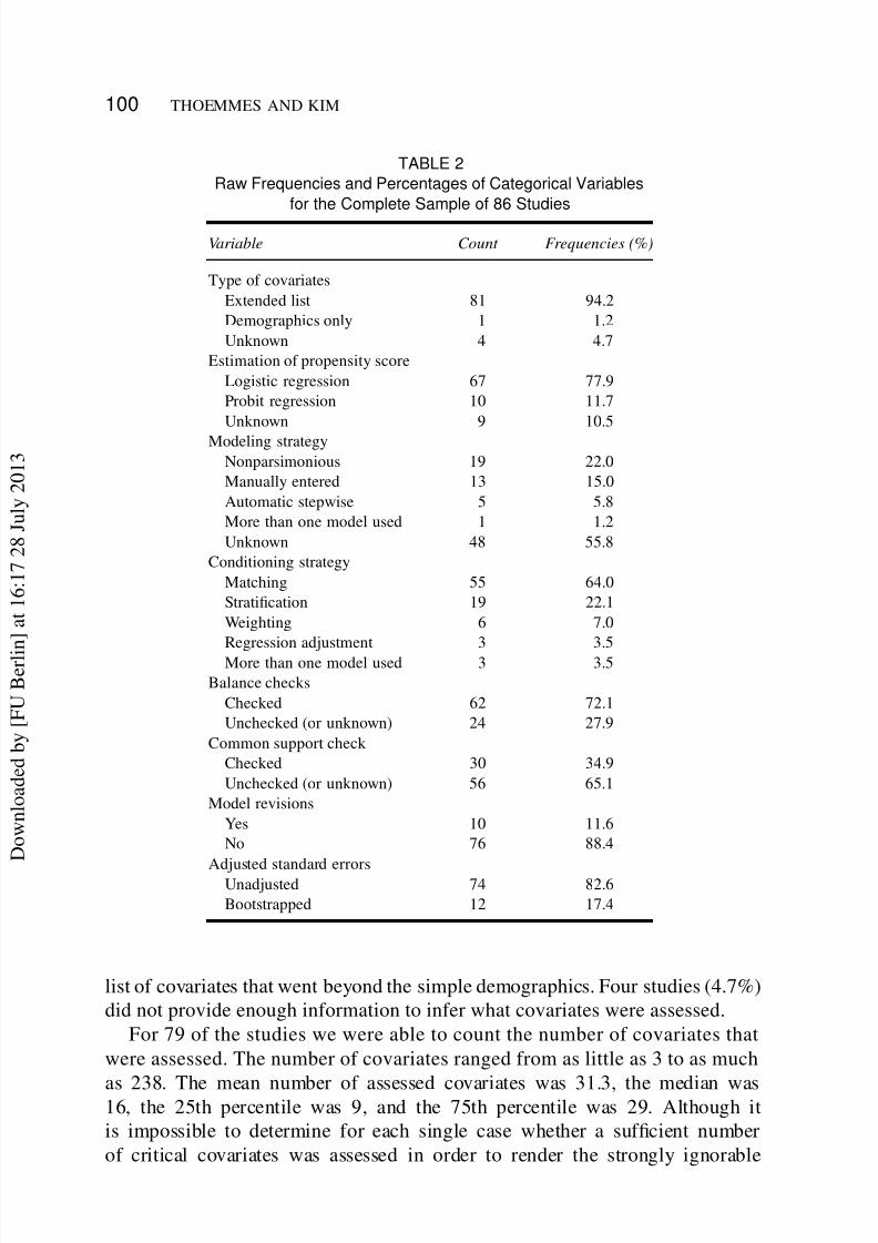
SYSTEMATIC REVIEW PROPENSITY SCORES 101
TABLE 3
Raw Frequencies and Percentages of Categorical Variables
for the 58 Studies That Used Matching
Variable Count Frequency (%)
Matching strategy
1:1 matching 25 43.1
1:many matching 18 31.0
More than one strategy used 9 15.5
Unknown 6 10.3
Matching strategy 2
Greedy matching 31 53.4
Other (e.g., optimal or kernel) 14 24.1
Unknown 13 22.4
Type of matching
Exact 1 1.7
Nearest neighbor 34 58.6
Other (e.g., kernel) 18 31.0
Unknown 5 8.6
treatment assignment assumption plausible, we believe that in only very few
cases will 3 variables be enough to convincingly control for all potential bi-ases. On the other side of the spectrum, more than 200 variables make a very
convincing case that potential bias due to unobserved confounding variables
is probably minimal. Generally speaking, it is encouraging to see that most
researchers exhibit an effort in collecting important covariates beyond purely
demographic variables. A point of criticism is that there were still 7 studies
TABLE 4
Raw Frequencies and Percentages of Categorical Variables forthe 62 Studies That Conducted Balance Checks
Variable Count Frequency (%)
Type of balance check
Significance test 41 66.1
Standard difference 14 22.6
Graphical 3 4.8
Raw difference 1 1.6
More than one approach 3 4.8
Balance variablesCovariates only 45 72.6
Propensity scores only 8 12.9
Propensity scores and covariates 9 14.5
D o w n l o a d e d b y [ F U B
e r l i
n ] a t 1 6 : 1 7 2 8 J u l y 2 0 1 3
7/27/2019 SisteMatic Review PsMt Ho Emmes
http://slidepdf.com/reader/full/sistematic-review-psmt-ho-emmes 15/31
102 THOEMMES AND KIM
TABLE 5
Descriptive Statistics of Continuous Variables for Relevant Studies With Observed Data
Variable Count % Reported M (SD)
Percentiles (25th,
Median, 75th)
Number of covariates
collected
79 91.9 31.3 (45.0) 9, 16, 29
Number of covariates entered
in final model
37 43.0 18.8 (13.9) 8, 16, 24
Caliper width (raw propensity
score)
9 33.3 .02 .01, .01, .05
Caliper width (SD of raw
propensity score)
4 14.8 .19 .15, .20, .25
Caliper width (SD of logit
propensity score)
5 18.5 .17 .10, .25, .25
Number of strata 19 90.5 8.26 5, 5, 10
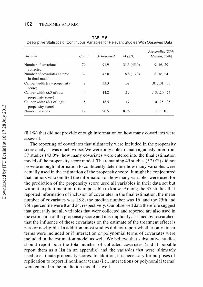
(8.1%) that did not provide enough information on how many covariates were
assessed.
The reporting of covariates that ultimately were included in the propensity
score analysis was much worse. We were only able to unambiguously infer from37 studies (43.0%) how many covariates were entered into the final estimation
model of the propensity score model. The remaining 49 studies (57.0%) did not
provide enough information to confidently determine how many variables were
actually used in the estimation of the propensity score. It might be conjectured
that authors who omitted the information on how many variables were used for
the prediction of the propensity score used all variables in their data set but
without explicit mention it is impossible to know. Among the 37 studies that
reported information of inclusion of covariates in the final estimation, the mean
number of covariates was 18.8, the median number was 16, and the 25th and75th percentile were 8 and 24, respectively. Our observed data therefore suggest
that generally not all variables that were collected and reported are also used in
the estimation of the propensity score and it is implicitly assumed by researchers
that the influence of these covariates on the estimate of the treatment effect is
zero or negligible. In addition, most studies did not report whether only linear
terms were included or if interaction or polynomial terms of covariates were
included in the estimation model as well. We believe that substantive studies
should report both the total number of collected covariates (and if possible
report them as a list in an appendix) and the variables that were ultimatelyused to estimate propensity scores. In addition, it is necessary for purposes of
replication to report if nonlinear terms (i.e., interactions or polynomial terms)
were entered in the prediction model as well.
D o w n l o a d e d b y [ F U B
e r l i
n ] a t 1 6 : 1 7 2 8 J u l y 2 0 1 3
7/27/2019 SisteMatic Review PsMt Ho Emmes
http://slidepdf.com/reader/full/sistematic-review-psmt-ho-emmes 16/31
SYSTEMATIC REVIEW PROPENSITY SCORES 103
Estimation of Propensity Score Models
The predominant mode of estimating the propensity score in our sample was
a logistic regression followed by probit regression. Sixty-seven studies (77.9%)
used logistic regression, and 10 studies (11.6%) used probit regression. The
remaining 9 studies (10.5%) did not provide enough information to discern
what model was used. Other methods, for example, discriminant analysis, or
regression trees were not used in our sample of studies. The logistic and probit
regression models are assumed to work reasonably well in many circumstances;
however, researchers should also be aware of more advanced models. McCaffrey
et al. (2004) provided information and accompanied software to use boosted
regression trees when estimating propensity scores. We encourage researchers
to explore these new methods as there is evidence that these methods can in
some circumstance yield better results (see McCaffrey et al., 2004). One of
the advantages of these algorithmic approaches is that any nonlinear terms are
automatically discovered and entered into the estimation model of the propen-
sity score.
Modeling Strategy
Overall reporting of choice of inclusion or exclusion of covariates in the modelwas lacking. Forty-eight studies (55.8%) did not provide enough information to
determine how covariates were chosen to be included in the estimation of the
propensity score. Five studies (5.8%) described using an automatic stepwise pro-
cedure (e.g., forward or backward stepwise regression). Thirteen studies (15.1%)
described various methods of picking covariates into the model that we describe
as manually entering terms. This includes examining bivariate relations between
covariates and treatment assignment and including only those that passed a
threshold of a prespecified significance level or manually adding and deleting
terms of a regression equation by examining significance of predictor terms dur-ing model building. Nineteen studies (22.1%) used a nonparsimonious approach
in which all available covariates were entered. This approach was primarily used
for studies that had only few variables. On average researchers that used the
nonparsimonious approach reported that they collected 27 covariates (median D
19, 25th percentile D 9.25, 75th percentile D 40.25), whereas in studies that
used stepwise procedures the average number of covariates was reported to be
83.3 (median D 54, 25th percentile D 18.75, 75th percentile D 177). Finally, a
single study presented two approaches and used both a nonparsimonious model
and a model in which terms were entered manually.We believe that there is a serious lack of reporting on modeling strategies that
are used to derive the final number of covariates in a model. Researchers should
be aware that exclusion of a covariate (by whichever means this was derived)
D o w n l o a d e d b y [ F U B
e r l i
n ] a t 1 6 : 1 7 2 8 J u l y 2 0 1 3
7/27/2019 SisteMatic Review PsMt Ho Emmes
http://slidepdf.com/reader/full/sistematic-review-psmt-ho-emmes 17/31
104 THOEMMES AND KIM
implies the conviction on the part of the researcher that this variable can be
ignored as a source of potential bias. Variables that are theoretically important
confounders should be included in the model regardless of statistical significance,and in addition balance should be checked on all available covariates even if
they were not included in the final estimation model.
Conditioning Strategy
Reporting on the general type of conditioning was overall satisfactory. Matching
(in its many variants) was the most popular choice (55 studies; 64.0%), followed
by stratification (19 studies; 22.1%), weighting (6 studies; 7.0%), and regression
adjustment in an ANCOVA type model (3 studies; 3.5%). Three studies (3.5%)used and reported more than one conditioning strategy. In detail, one study used
both matching and regression adjustment, and two studies used both matching
and stratification.
Aspects of Matching
We assessed several important aspects of matching. First we determined what
type of matching was used. Out of the 58 studies that used matching (note
that this includes studies that used multiple conditioning methods, including
matching), 6 studies (10.3%) did not report what type of matching was used.
Twenty-five studies (43.1%) used 1:1 matching exclusively, and 18 studies
(31.0%) used 1:many matching. A total of 9 studies (15.5%) used and reported
several matching strategies. In detail, 6 studies (10.3%) used both 1:1 and 1:many
matching; 2 studies (3.4%) used 1:1 matching and a second matching strategy
categorized as “other” (e.g., kernel matching); and 1 study (1.7%) used 1:1
matching, 1:many matching, and a third “other” strategy.2 Overall, this aspect
of reporting was also satisfactory.
A second aspect of matching that we coded was whether greedy matching or
a different kind of matching (e.g., optimal or kernel matching) was performed.
Thirty-one studies (53.4%) used the simple greedy algorithm, whereas 14 studies
(24.1%) relied on other algorithmic approaches, such as optimal matching, or
kernel matching. The remaining 13 studies (22.4%) did not provide enough
information about their matching strategy. Another aspect of matching that
we assessed was whether a study that used matching relied on exact, nearest
neighbor or a different algorithm (e.g., kernel matching). A single study used
exact matching on the propensity score, 34 studies (58.6%) used nearest neighbor
matching, and 18 studies (31%) used other approaches (e.g., kernel matching).
2The “other” category was introduced because counts in several categories were very low and
reliability suffered when these categories were considered separately.
D o w n l o a d e d b y [ F U B
e r l i
n ] a t 1 6 : 1 7 2 8 J u l y 2 0 1 3
7/27/2019 SisteMatic Review PsMt Ho Emmes
http://slidepdf.com/reader/full/sistematic-review-psmt-ho-emmes 18/31
SYSTEMATIC REVIEW PROPENSITY SCORES 105
The remaining 5 studies (8.6%) did not provide enough information to determine
what type of matching was used. Among the 34 studies that used nearest
neighbor matching, we checked whether or not researchers reported that they hadused a caliper. Twenty-seven studies (79.4%) of the 34 studies that used nearest
neighbor matching reported using a caliper. The other 7 studies (20.59%) did
not report using any caliper. In an attempt to look more closely at how calipers
are used in applied research, we recorded whether researchers reported the scale
and the width of the caliper. Out of the 27 studies that reported that they have
used a caliper, 9 studies (33.3%) failed to report the crucial information of what
kind of caliper they used. The remaining 18 studies (66.7%) fortunately included
this information. Nine studies (33.3%) reported that they used a caliper based
on the raw propensity score. The most frequently chosen value (5 studies) was.01; on average the caliper width on the raw propensity score scale was .02.
Four studies (14.8%) used a caliper based on the standard deviation of the raw
propensity score. The width of this caliper ranged from .10 to .25. Finally, 5
studies (18.5%) used a caliper width based on the standard deviation of the logit
of the propensity score. The most frequently used caliper (3 studies) had a width
of .25.
Finally, we tried to assess the percentage of units retained after matching.
Specifically, we wanted to know how large the overall sample size of any given
study was before and after the matching procedure. Surprisingly this informationwas often not reported or had to be inferred from changes in degrees of freedom
in statistical tests. For the 25 studies that provided this information, we were
unable to achieve acceptable reliability between our two coders. Sample sizes
before and after matching often had to be inferred from differences in degrees
of freedom and in our study this turned out to be error prone. It is unfortunate
that we were unable to reliably assess sample sizes before and after matching.
Reporting actual sample sizes before and after matching (and not just degrees
of freedom of tests conducted before and after matching) would help readers to
assess these percentages more easily.Overall, we feel that as long as researchers reported their strategies, many
of them used defensible choices. Only a few studies employed techniques that
would be considered unorthodox (e.g., a single study used an extremely small
caliper width of .0005). The biggest problem was the substantial amount of
underreporting of specific details. It was also interesting to see that there was a
large amount of variability in approaches starting from type of matching, number
of units matched, or the caliper width. None of these characteristics were used
uniformly across all studies. Although we generally believe that pluralism in
approaches is not necessarily bad (e.g., different data situations might call forslightly different approaches), this heterogeneity makes it somewhat hard for
other researchers to replicate findings as they may be the result of idiosyncratic
choices.
D o w n l o a d e d b y [ F U B
e r l i
n ] a t 1 6 : 1 7 2 8 J u l y 2 0 1 3
7/27/2019 SisteMatic Review PsMt Ho Emmes
http://slidepdf.com/reader/full/sistematic-review-psmt-ho-emmes 19/31
106 THOEMMES AND KIM
Aspects of Stratification
Out of the 21 studies that used stratification, 2 studies (9.5%) did not report
the number of strata that were used. By far the most common choice of strata
was 5 (as prescribed by Cochran, 1968), which was used by 10 studies (47.6%).
Two studies (9.5%) used 6 strata, 3 studies (14.3%) used 10 strata, another 3
studies (14.3%) used 15 strata, and 1 study (4.8%) used 20 strata. The original
recommendation of 5 strata is a useful rule of thumb that was demonstrated to
remove nearly 90% of linear bias of a single covariate (Cochran, 1968). However,
in the context of propensity score modeling, researchers should test whether
the chosen number of strata actually balances covariates when conditioning on
strata membership. If balance is not achieved, a larger number of strata might
be needed.
Aspects of Weighting and ANCOVA
Weighting and ANCOVA were not frequently used. The six studies that used
weighting relied on the inverse probability weights as described previously.
The three studies that used regression adjustment used the propensity score
as a covariate. The additional assumptions that accompany this approach were
described earlier.
Aspects of Balance Checks and Common Support
We were especially interested in determining whether researchers conducted
and reported model adequacy checks such as balance checks and checks on the
common support region. A majority of 62 studies (72.1%) conducted some sort
of balance checks, whereas the remaining studies (24; 27.9%) failed to report
it. It is possible, though we believe not likely, that these studies conducted
balance checks but simply chose not to report them. We note at this point thatthe percentage of studies in the social sciences that conducted the important
balance checks was higher than the percentage of medical studies as reported in
Austin (2008b).
We also examined how researchers tested for balance. Out of the 62 studies
that did check for balance, a large number of studies (41 studies; 66.1%)
used only significance tests, meaning that researchers computed a t or chi-
square statistic for each covariate after matching and decided based on a p
value whether or not balance was achieved. Fourteen studies (22.6%) assessed
only standardized differences on covariates between groups; 3 studies (4.8%)presented a form of graphical comparison (either Q-Q plots or comparative
distribution graphics such as box plots, histograms, or kernel density estimates).
A single study (1.6%) reported raw differences on covariates. Several studies (3;
D o w n l o a d e d b y [ F U B
e r l i
n ] a t 1 6 : 1 7 2 8 J u l y 2 0 1 3
7/27/2019 SisteMatic Review PsMt Ho Emmes
http://slidepdf.com/reader/full/sistematic-review-psmt-ho-emmes 20/31
SYSTEMATIC REVIEW PROPENSITY SCORES 107
4.8%) used and reported more than one method for balance checks. In detail,
one study used significance tests and standardized differences together; one
study used a graph and standardized differences together; and finally one studyused significance tests, standardized differences, and a graph. All studies in
our sample only reported balance statistics (whether in the form of significance
tests or standardized differences) on mean levels but never on variances of the
covariates. We also coded whether a study checked balance (in whatever form)
only on the propensity score as a summary measure or if individual covariates
were checked for balance. We found that among the 62 studies that checked for
balance, 8 studies (12.9%) checked balance on the propensity score alone, 45
studies (72.6%) checked balance on the covariates only, and 9 studies (14.5%)
checked balance on both the covariates and the propensity score.In a next step, we observed that most researchers did not report checks on the
common support region. In 30 studies (34.9%) we found explicit mentioning of
the common support region. In the other 56 studies (65.1%), we did not find any
reporting on this matter. Again, we cannot rule out the possibility that researchers
checked the common support region and chose not to report it, but we believe
that this is unlikely.
Finally, we checked whether researchers reported that the propensity score
model was respecified if imbalances were found. A respecification of the model
would be the appropriate step to engage in if large imbalances would be found.We observed that only 10 studies (11.6%) reported revising a model when imper-
fect balance was found. Other studies gave no indication whether or not models
were respecified. We are again not sure as to whether the remaining studies
simply did not report whether a model was reestimated in order to not overburden
the reader or if they simply ignored potential imbalances. Researchers should
be aware that the first estimated propensity score model (which usually only
includes linear terms) can fail to achieve balance on the observed covariates and
needs to be reestimated with additional terms (e.g., interactions or polynomial
terms). In regard to reporting and use of model checks we make the followingobservations: Given the tremendous importance of the balance property, the
fact that almost 30% of studies did not check for balance is disappointing.
A propensity score analysis without the balance checks can be based on a
misspecified model and such a model cannot be expected to properly control for
all potential biases on the observed covariates. We urge researchers to engage
in balance checks and proper reporting of those checks every time a propensity
score analysis is conducted. We further suggest that researchers rely on the
assessment of standardized differences. The use of significance tests can in some
circumstances be erroneous because imbalances might not be detected due tolower statistical power. Standardized differences do not confound balance with
other factors and are the preferred method. Graphical comparisons as described
earlier can be used in the estimation and conditioning phase of the propensity
D o w n l o a d e d b y [ F U B
e r l i
n ] a t 1 6 : 1 7 2 8 J u l y 2 0 1 3
7/27/2019 SisteMatic Review PsMt Ho Emmes
http://slidepdf.com/reader/full/sistematic-review-psmt-ho-emmes 21/31
108 THOEMMES AND KIM
score analysis as a quick way to gauge large imbalances, but we endorse using
them only in conjunction with examination of standardized differences.
We encourage researchers to examine the common support region as it relatesclosely to generalizability of results. Although it might not always be necessary
to present graphs, we do believe that researchers should report in which range
of the propensity score distribution relevant matches could be found and which
region of the propensity score distribution had to be discarded.
Adjusted Standard Errors
In our sample we found no explicit mentioning of standard errors that were ad-
justed for the matched nature of the data (e.g., using dependent samples t tests).However, we found several studies (12; 14.0%) that reported using bootstrap
standard error. Bootstrapped standard errors are often used in circumstances
in which a theoretical sampling distribution is unknown, however, Abadie and
Imbens (2008) recently argued that the bootstrap is an inappropriate method for
matched data. Therefore bootstrapping cannot be unconditionally recommended
in the context of propensity score matching.
DISCUSSION
Overall, we think that both good but also suboptimal practice exists with regard
to propensity score analysis. On the one hand, we are pleased to see that
researchers in the social sciences are exploring new methodological tools in their
substantive research. On the other hand, there are some clear deficiencies in the
use of propensity scores. Some of these deficiencies are related to poor reporting
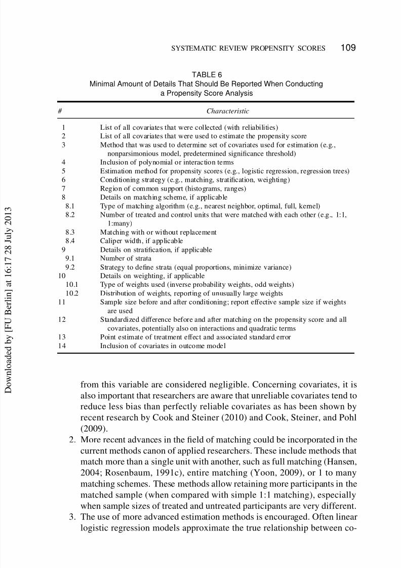
practices. We provide applied researchers with a list of the minimal amount of
details that should be reported in a propensity score analysis in Table 6.
Areas in which positive practice dominates are reporting practices of esti-mation choices and the general conditioning strategy. Also, the fact that most
researchers do not simply use demographics to conduct post hoc propensity
score analyses is a sign of good practice. Many of the choices, when reported,
were often sensible, for example, the often used logistic regression equation
followed by a simple 1:1 matching scheme. Areas of improvement on the use
and reporting of propensity score methods are the following:
1. Researchers should make very clear which variables were collected and
even more important which ones were actually included in the estimationof the propensity score. Appendices that list variables are recommended.
There should be an increased awareness that omission of variables in
the propensity score estimation implicitly assumes that potential biases
D o w n l o a d e d b y [ F U B
e r l i
n ] a t 1 6 : 1 7 2 8 J u l y 2 0 1 3
7/27/2019 SisteMatic Review PsMt Ho Emmes
http://slidepdf.com/reader/full/sistematic-review-psmt-ho-emmes 22/31
SYSTEMATIC REVIEW PROPENSITY SCORES 109
TABLE 6
Minimal Amount of Details That Should Be Reported When Conducting
a Propensity Score Analysis
# Characteristic
1 List of all covariates that were collected (with reliabilities)
2 List of all covariates that were used to estimate the propensity score
3 Method that was used to determine set of covariates used for estimation (e.g.,
nonparsimonious model, predetermined significance threshold)
4 Inclusion of polynomial or interaction terms
5 Estimation method for propensity scores (e.g., logistic regression, regression trees)
6 Conditioning strategy (e.g., matching, stratification, weighting)
7 Region of common support (histograms, ranges)
8 Details on matching scheme, if applicable8.1 Type of matching algorithm (e.g., nearest neighbor, optimal, full, kernel)
8.2 Number of treated and control units that were matched with each other (e.g., 1:1,
1:many)
8.3 Matching with or without replacement
8.4 Caliper width, if applicable
9 Details on stratification, if applicable
9.1 Number of strata
9.2 Strategy to define strata (equal proportions, minimize variance)
10 Details on weighting, if applicable
10.1 Type of weights used (inverse probability weights, odd weights)
10.2 Distribution of weights, reporting of unusually large weights
11 Sample size before and after conditioning; report effective sample size if weights
are used
12 Standardized difference before and after matching on the propensity score and all
covariates, potentially also on interactions and quadratic terms
13 Point estimate of treatment effect and associated standard error
14 Inclusion of covariates in outcome model
from this variable are considered negligible. Concerning covariates, it is
also important that researchers are aware that unreliable covariates tend toreduce less bias than perfectly reliable covariates as has been shown by
recent research by Cook and Steiner (2010) and Cook, Steiner, and Pohl
(2009).
2. More recent advances in the field of matching could be incorporated in the
current methods canon of applied researchers. These include methods that
match more than a single unit with another, such as full matching (Hansen,
2004; Rosenbaum, 1991c), entire matching (Yoon, 2009), or 1 to many
matching schemes. These methods allow retaining more participants in the
matched sample (when compared with simple 1:1 matching), especiallywhen sample sizes of treated and untreated participants are very different.
3. The use of more advanced estimation methods is encouraged. Often linear
logistic regression models approximate the true relationship between co-
D o w n l o a d e d b y [ F U B
e r l i
n ] a t 1 6 : 1 7 2 8 J u l y 2 0 1 3
7/27/2019 SisteMatic Review PsMt Ho Emmes
http://slidepdf.com/reader/full/sistematic-review-psmt-ho-emmes 23/31
110 THOEMMES AND KIM
variates and treatment assignment well; however, the inclusion of nonlinear
terms (interactions and polynomials) can improve the selection model.
Methods such as boosted regression trees (McCaffrey et al., 2004) or ge-netic matching (Diamond & Sekhon, 2005) attempt to find these complex
relationships by applying automatic data mining algorithms.
4. Balance checks should be conducted by examining standardized differ-
ences before and after matching on all covariates that were collected in
the data set. The practice of using significance tests is still very widespread
and an appreciation of the fact that nonsignificant results can just emerge
out of reduced sample sizes (and not increased balance) is necessary. Even
though there is no generally accepted cutoff for what constitutes a critical
imbalance on the standardized difference metric, nontrivial standardizeddifferences should be considered problematic and should trigger the re-
searcher to reestimate the model or apply a more stringent conditioning
scheme (e.g., smaller calipers, more strata). Generally, the smaller the
standardized difference is, the less likely this covariate is to exert any
residual bias on the treatment effect. Austin (2009a) provides advice
on how to determine a range of standardized differences that would be
expected by chance to provide researchers with an idea of the magnitude
of difference that is likely acceptable.
5. The common support region should be examined and implications regard-ing generalizability should be addressed by the researcher. A small area of
common support informs the researcher that the observed causal effect is
only valid for a small subpopulation of the observed sample and unlikely
to generalize to other populations. Large areas of common support, on the
other hand, increase one’s faith that the observed effect is valid for the
whole population that is being represented by the sample at hand. Common
support checks can be conducted graphically or simply by examining the
range of matched and unmatched participants.
Propensity score methodology and associated procedures are most likely
going to stay with us as statistical tools in applied social science research.
It is of importance that as a field we strive to use these methods in the most
appropriate fashion, incorporate new developments, and report our analyses in
a way that makes them replicable for future researchers.
ACKNOWLEDGMENTS
Felix J. Thoemmes is now at the University of Tübingen, Germany. We thank
Elizabeth Stuart for her feedback on earlier versions of this article.
D o w n l o a d e d b y [ F U B
e r l i
n ] a t 1 6 : 1 7 2 8 J u l y 2 0 1 3
7/27/2019 SisteMatic Review PsMt Ho Emmes
http://slidepdf.com/reader/full/sistematic-review-psmt-ho-emmes 24/31
SYSTEMATIC REVIEW PROPENSITY SCORES 111
REFERENCES
Abadie, A., & Imbens, G. W. (2008). On the failure of the bootstrap for matching estimators. Econometrica, 76, 1537–1557. doi:10.3982/ecta6474
Austin, P. (2007). Propensity-score matching in the cardiovascular surgery literature from 2004
to 2006: A systematic review and suggestions for improvement. The Journal of Thoracic and
Cardiovascular Surgery, 134, 1128–1135.
Austin, P. (2008a). A critical appraisal of propensity-score matching in the medical literature between
1996 and 2003. Statistics in Medicine, 27, 2037–2049.
Austin, P. (2008b). Primer on statistical interpretation or methods report card on propensity-score
matching in the cardiology literature from 2004 to 2006: A systematic review. Circulation-
Cardiovascular Quality and Outcomes, 1, 62–67.
Austin, P. (2009a). Balance diagnostics for comparing the distribution of baseline covariates between
treatment groups in propensity-score matched samples. Statistics in Medicine, 28, 3083–3107.Austin, P. (2009b). Type I error rates, coverage of confidence intervals, and variance estimation in
propensity-score matched analyses. The International Journal of Biostatistics, 5, 13–38.
Caliendo, M., & Kopeinig, S. (2008). Some practical guidance for the implementation of propensity
score matching. Journal of Economic Surveys, 22, 31–72.
Cochran, W. G. (1968). The effectiveness of adjustment by subclassification in removing bias in
observational studies. Biometrics, 24, 295–313.
Cohen, J. (1988). Statistical power analysis for the behavioral sciences. Hillsdale, NJ: Erlbaum.
Cook, T. D., & Steiner, P. (2010). Case matching and the reduction of selection bias in quasi-
experiments: The relative importance of pretest measures of outcome, of unreliable measurement,
and of mode of data analysis. Psychological Methods, 15, 56–86. doi:10.1037/a0018536
Cook, T. D., Steiner, P., & Pohl, S. (2009). How bias reduction is affected by covariate choice,unreliability, and mode of data analysis: results from two types of within-study comparisons.
Multivariate Behavioral Research, 44, 828–847. doi:10.1080/00273170903333673
Diamond, A., & Sekhon, J. (2005). Genetic matching for estimating causal effects: A new method
of achieving balance in observational studies. Retrieved from http://jsekhon.fas.harvard.edu/
Gu, X., & Rosenbaum, P. R. (1993). Comparison of multivariate matching methods: Structures,
distances, and algorithms. Journal of Computational and Graphical Statistics, 2, 405–420.
Hansen, B. B. (2004). Full matching in an observational study of coaching for the SAT. Journal of
the American Statistical Association, 99, 609–619.
Hansen, B. (2008). The essential role of balance tests in propensity-matched observational studies:
Comments on ‘A critical appraisal of propensity-score matching in the medical literature between
1996 and 2003’ by Peter Austin. Statistics in Medicine, 27, 2050–2054.Haviland, A., Nagin, D., & Rosenbaum, P. R. (2007). Combining propensity score matching and
group-based trajectory analysis in an observational study. Psychological Methods, 12, 247–267.
Hayes, A. F., & Krippendorff, K. (2007). Answering the call for a standard reliability measure for
coding data. Communication Methods and Measures, 1, 77–89.
Heckman, J. J., Ichimura, H., & Todd, P. E. (1997). Matching as an econometric evaluation estimator:
Evidence from evaluating a job training programme. The Review of Economic Studies, 64, 605–
654.
Heckman, J., Ichimura, H., & Todd, P. (1998). Matching as an econometric evaluation estimator.
The Review of Economic Studies, 65, 261–294.
Helmreich, J., & Pruzek, R. M. (2009) PSAgraphics: An R package to support propensity score
analysis. Journal of Statistical Software, 29. Retrieved from http://www.jstatsoft.org/v29/i06/ paper
Hill, J. (2008). Discussion of research using propensity-score matching: Comments on ‘A critical
appraisal of propensity-score matching in the medical literature between 1996 and 2003’ by Peter
Austin. Statistics in Medicine, 27, 2055–2061.
D o w n l o a d e d b y [ F U B
e r l i
n ] a t 1 6 : 1 7 2 8 J u l y 2 0 1 3
7/27/2019 SisteMatic Review PsMt Ho Emmes
http://slidepdf.com/reader/full/sistematic-review-psmt-ho-emmes 25/31
112 THOEMMES AND KIM
Hirano, K., & Imbens, G. (2001). Estimation of causal effects using propensity score weighting:
An application to data on right heart catheterization. Health Services and Outcomes Research
Methodology, 2, 259–278.
Hirano, K., Imbens, G. W., & Ridder, G. (2003). Efficient estimation of average treatment effects
using the estimated propensity score. Econometrica, 71, 1161–1189.
Ho, D. E., Imai, K., King, G., & Stuart, E. A. (2007). Matching as nonparametric preprocessing for
reducing model dependence in parametric causal inference. Political Analysis, 15, 199–236. doi:
10.1093/pan/mpl013
Hong, G., & Raudenbush, S. (2005). Effects of kindergarten retention policy on children’s cognitive
growth in reading and mathematics. Educational Evaluation and Policy Analysis, 27, 205–224.
Hughes, J., Chen, Q., Thoemmes, F., & Kwok, O. (2010). Effect of retention in first grade on
performance on high stakes test in 3rd grade. Educational Evaluation and Policy Analysis, 32,
166–182.
Hullsiek, K., & Louis, T. (2002). Propensity score modeling strategies for the causal analysis of
observational data. Biostatistics, 3, 179–193.
Imai, K., King, G., & Stuart, E. (2008). Misunderstandings among experimentalists and observa-
tionalists about causal inference. Journal of the Royal Statistical Society, Series A, 171, 481–502.
Kang, J., & Schafer, J. (2007). Demystifying double robustness: a comparison of alternative strategies
for estimating a population mean from incomplete data. Statistical Science, 22, 523–539.
King, G., & Zeng, L. (2007). When can history be our guide? The pitfalls of counterfactual inference.
International Studies Quarterly, 51, 183–210.
Krippendorff, K. (2004). Reliability in content analysis. Human Communication Research, 30, 411–
433.
Lunceford, J., & Davidian, M. (2004). Stratification and weighting via the propensity score in
estimation of causal treatment effects: A comparative study. Statistics in Medicine, 23, 2937–
2960.
McCaffrey, D., Ridgeway, G., & Morral, A. (2004). Propensity score estimation with boosted
regression for evaluating causal effects in observational studies. Psychological Methods, 9, 403–
425.
Ming, K., & Rosenbaum, P. R. (2000). Substantial gains in bias reduction from matching with a
variable number of controls. Biometrics, 56, 118–124.
Ming, K., & Rosenbaum, P. R. (2001). A note on optimal matching with variable controls using the
assignment algorithm. Journal of Computational & Graphical Statistics, 10, 455–463.
Myers, J. A., & Louis, T. A. (2007). Optimal propensity score stratification. Johns Hopkins Univer-
sity, Department of Biostatistics Working Papers (Working Paper No. 155). Retrieved from http://
www.bepress.com/jhubiostat/paper155
Robins, J., Rotnitzky, A., & Scharfstein, D. (1999). Sensitivity analysis for selection bias and
unmeasured confounding in missing data and causal inference models. In M. R. Halloran &
D. Berry (Eds.), Statistical models in epidemiology: The environment and clinical trials (pp.
1–92). New York, NY: Springer.
Rosenbaum, P. R. (1989). Optimal matching for observational studies. Journal of the American
Statistical Association, 84, 1024–1032.
Rosenbaum, P. R. (1991a). Sensitivity analysis for matched case-control studies. Biometrics, 47,
87–100.
Rosenbaum, P. R. (1991b). Discussing hidden bias in observational studies. Annals of Internal
Medicine, 115, 901–905.
Rosenbaum, P. R. (1991c). A characterization of optimal designs for observational studies. Journal
of the Royal Statistical Society, Series B (Methodological), 53, 597–610.
Rosenbaum, P. R. (2010). Design of observational studies. New York, NY: Springer.
Rosenbaum, P. R., & Rubin, D. B. (1983). The central role of the propensity score in observational
studies for causal effects. Biometrika, 70, 41–55.
D o w n l o a d e d b y [ F U B
e r l i
n ] a t 1 6 : 1 7 2 8 J u l y 2 0 1 3
7/27/2019 SisteMatic Review PsMt Ho Emmes
http://slidepdf.com/reader/full/sistematic-review-psmt-ho-emmes 26/31
SYSTEMATIC REVIEW PROPENSITY SCORES 113
Rosenbaum, P., & Rubin, D. B. (1984). Reducing bias in observational studies using subclassification
on the propensity score. Journal of the American Statistical Association, 79, 516–524.
Rosenbaum, P., & Rubin, D. B. (1985). Constructing a control group using multivariate matched
sampling methods that incorporate the propensity score. American Statistician, 39, 33–38.
Rubin, D. (2005). Causal inference using potential outcomes. Journal of the American Statistical
Association, 100, 322–331.
Rubin, D. B., & Thomas, N. (1992). Characterizing the effect of matching using linear propensity
score methods with normal distributions. Biometrika, 79, 797–809.
Rubin, D. B., & Thomas, N. (1996). Matching using estimated propensity scores: Relating theory
to practice. Biometrics, 52, 249–264.
Rubin, D. B., & Waterman, R. P. (2006). Estimating the casual effects of marketing interventions
using propensity score methodology. Statistical Science, 21, 206–222.
Schafer, J. L., & Kang, J. (2008). Average causal effects from nonrandomized studies: A practical
guide and simulated example. Psychological Methods, 13, 279–313.
Shadish, W., Luellen, J., & Clark, M. (2006). Propensity scores and quasi-experiments: A testimony
to the practical side of Lee Sechrest. In R. R. Bootzin & P. E. McKnight (Eds.), Strengthening
research methodology: Psychological measurement and evaluation (pp. 143–157). Washington,
DC: American Psychological Association.
Shadish, W., & Steiner, P. (2010). A primer on propensity score analysis. Newborn and Infant
Nursing Reviews, 10, 19–26.
Stuart, E. (2008). Developing practical recommendations for the use of propensity scores: Discussion
of ‘A critical appraisal of propensity score matching in the medical literature between 1996 and
2003’ by Peter Austin. Statistics in Medicine, 27, 2062–2065.
Stuart, E. (2010). Matching methods for causal inference: A review and a look forward. Statistical
Science, 25, 1–21.
Stuart, E., Marcus, S., Horvitz-Lennon, M., Gibbons, R., Normand, S., & Brown, H. (2009). Using
non-experimental data to estimate treatment effects. Psychiatric Annals, 39, 719–728.
Tukey, J. W. (1977). Exploratory data analysis. Reading. MA: Addison-Wesley.
Weitzen, S., Lapane, K., Toledano, A., Hume, A., & Mor, V. (2004). Principles for modeling
propensity scores in medical research: A systematic literature review. Pharmacoepidemiology
and Drug Safety, 13, 841–853.
Wu, W., West, S., & Hughes, J. (2008). Short-term effects of grade retention on the growth rate of
Woodcock-Johnson III broad math and reading scores. Journal of School Psychology, 46 , 85–105.
Yoon, F. (2009). Entire matching and its application in an observational study of treatments for
melanoma. Unpublished manuscript.
APPENDIX
References Used in the Systematic Literature Review
Amato, P. R. (2003). Reconciling divergent perspectives: Judith Wallerstein, quantitative family
research, and children of divorce. Family Relations, 52, 332–339.
Anand, P., Mizala, A., & Repetto, A. (2009). Using school scholarships to estimate the effect of
private education on the academic achievement of low-income students in Chile. Economics of
Education Review, 28, 370–381.
Aassve, A., Davia, M. A., Iacovou, M., & Mazzuco, S. (2007). Does leaving home make you poor?
Evidence from 13 European countries. European Journal of Population-Revue Europeenne De
Demographie, 23, 315–338. doi:10.1007/s10680-007-9135-5
D o w n l o a d e d b y [ F U B
e r l i
n ] a t 1 6 : 1 7 2 8 J u l y 2 0 1 3
7/27/2019 SisteMatic Review PsMt Ho Emmes
http://slidepdf.com/reader/full/sistematic-review-psmt-ho-emmes 27/31
114 THOEMMES AND KIM
Attewell, P., & Domina, T. (2008). Raising the bar: Curricular intensity and academic performance.
Educational Evaluation and Policy Analysis, 30, 51–71. doi:10.3102/0162373707313409
Attewell, P., Lavin, D., Domina, T., & Levey, T. (2006). New evidence on college remediation.
Journal of Higher Education, 77, 886–924.
Barth, R. P., Guo, S., & McCrae, J. S. (2008). Propensity score matching strategies for evaluating
the success of child and family service programs. Research on Social Work Practice, 18, 212–222.
doi:10.1177/1049731507307791
Barth, R. P., Lee, C. K., Wildfire, J., & Guo, S. Y. (2006). A comparison of the governmental costs
of long-term foster care and adoption. Social Service Review, 80, 127–158.
Bellamy, J. L. (2008). Behavioral problems following reunification of children in long-term foster
care. Children and Youth Services Review, 30, 216–228. doi:10.1016/j.childyouth.2007.09.008
Bennett, P. R., & Lutz, A. (2009). How African American is the net Black advantage? Differences in
college attendance among immigrant Blacks, native Blacks, and Whites. Sociology of Education,
82, 70–99.
Berger, L., Brooks-Gunn, J., Paxson, C., & Waldfoge, J. (2008). First-year maternal employment
and child outcomes: Differences across racial and ethnic groups. Children and Youth Services
Review, 30, 365–387. doi:10.1016/j.childyouth.2007.10.010
Brand, J. E., & Halaby, C. N. (2006). Regression and matching estimates of the effects of elite
college attendance on educational and career achievement. Social Science Research, 35, 749–770.
doi:10.1016/j.ssresearch.2005.06.006
Caldwell, M. F., Vitacco, M., & Van Rybroek, G. J. (2006). Are violent delinquents worth treat-
ing? A cost-benefit analysis. Journal of Research in Crime and Delinquency, 43, 148–168.
doi:10.1177/0022427805280053
Callahan, R., Wilkinson, L., & Muller, C. (2008). School context and the effect of ESL placement
on Mexican-origin adolescents’ achievement. Social Science Quarterly, 89, 177–198.
Callahan, R., Wilkinson, L., Muller, C., & Frisco, M. (2009). ESL placement and schools: Effects
on immigrant achievement. Educational Policy, 23, 355–384. doi:10.1177/0895904807310034
Camp, S. D., Daggett, D. M., Kwon, O., & Klein-Saffran, J. (2008). The effect of faith program
participation on prison misconduct: The Life Connections Program. Journal of Criminal Justice,
36, 389–395. doi:10.1016/j.jcrimjus.2008.07.004
Casanueva, C., Martin, S. L., Runyan, D. K., Barth, R. P., & Bradley, R. H. (2008). Parenting
services for mothers involved with child protective services: Do they change maternal parenting
and spanking behaviors with young children? Children and Youth Services Review, 30, 861–878.
doi:10.1016/j.childyouth.2007.12.013
Condron, D. J. (2008). An early start: Skill grouping and unequal reading gains in the elementary
years. Sociological Quarterly, 49, 363–394.
Correnti, R. (2007). An empirical investigation of professional development effects on literacy in-
struction using daily logs. Educational Evaluation and Policy Analysis, 29, 262–295. doi:10.3102/
0162373707309074
Crosnoe, R. (2005). Double disadvantage or signs of resilience? The elementary school contexts of
children from Mexican immigrant families. American Educational Research Journal, 42, 269–303.
Crosnoe, R. (2009). Family-school connections and the transitions of low-income youths and English
language learners from middle school to high school. Developmental Psychology, 45, 1061–1076.
doi:10.1037/a0016131
Dahl, E., & Lorentzen, T. (2005). What works for whom? An analysis of active labour market
programmes in Norway. International Journal of Social Welfare, 14, 86–98.
Delander, L., Hammarstedt, M., Mansson, J., & Nyberg, E. (2005). Integration of immigrants: The
role of language proficiency and experience. Evaluation Review, 29, 24–41.
Delisi, M., Barnes, J. C., Beaver, K. M., & Gibson, C. L. (2009). Delinquent gangs and adolescent
victimization revisited: A propensity score matching approach. Criminal Justice and Behavior,
36, 808–823. doi:10.1177/0093854809337703
D o w n l o a d e d b y [ F U B
e r l i
n ] a t 1 6 : 1 7 2 8 J u l y 2 0 1 3
7/27/2019 SisteMatic Review PsMt Ho Emmes
http://slidepdf.com/reader/full/sistematic-review-psmt-ho-emmes 28/31
SYSTEMATIC REVIEW PROPENSITY SCORES 115
DeSena, A. D., Murphy, R. A., Douglas-Palumberi, H., Blau, G., Kelly, B., Horwitz, S. M., &
Kaufman, J. (2005). Safe homes: Is it worth the cost? Child Abuse and Neglect: The International
Journal, 29, 627–643.
Diaz, J. J., & Handa, S. (2006). An assessment of propensity score matching as a nonexperimental
impact estimator: Evidence from Mexico’s PROGRESA program. Journal of Human Resources,
41, 319–345.
Dill, J. S. (2009). Preparing for public life: School sector and the educational context of lasting
citizen formation. Social Forces, 87, 1265–1290.
Domina, T. (2009). What works in college outreach: Assessing targeted and schoolwide inter-
ventions for disadvantaged students. Educational Evaluation and Policy Analysis, 31, 127–152.
doi:10.3102/0162373709333887
Doyle, W. R. (2009). The effect of community college enrollment on bachelor’s degree completion.
Economics of Education Review, 28 , 199–206. doi:10.1016/j.econedurev.2008.01.006
Foster, E. M., Stephens, R., Krivelyova, A., & Gamfi, P. (2007). Can system integration improve
mental health outcomes for children and youth? Children and Youth Services Review, 29, 1301–
1319. doi:10.1016/j.childyouth.2007.05.004
Frank, K. A., Sykes, G., Anagnostopoulos, D., Cannata, M., Chard, L., Krause, A., &
McCrory, R. (2008). Does NBPTS certification affect the number of colleagues a teacher helps
with instructional matters? Educational Evaluation and Policy Analysis, 30, 3–30. doi:10.3102/
0162373707313781
Frisco, M. L., Muller, C., & Frank, K. (2007). Parents’ union dissolution and adolescents’ school
performance: Comparing methodological approaches. Journal of Marriage and the Family, 69,
721–741.
Furstenberg, F. F., Jr., & Neumark, D. (2007). Encouraging education in an urban school district:
Evidence from the Philadelphia educational longitudinal study. Education Economics, 15(2), 135–
157.
Gangl, M. (2006). Scar effects of unemployment: An assessment of institutional complementarities.
American Sociological Review, 71, 986–1013.
Gibson-Davis, C. M., & Foster, E. M. (2006). A cautionary tale: Using propensity scores to estimate
the effect of food stamps on food insecurity. Social Service Review, 80, 93–126.
Green, K. M., & Ensminger, M. E. (2006). Adult social behavioral effects of heavy adolescent
marijuana use among African Americans. Developmental Psychology, 42, 1168–1178.
Grunwald, H. E., & Mayhew, M. J. (2008). Using propensity scores for estimating causal effects:
A study in the development of moral reasoning. Research in Higher Education, 49, 758–775.
Hahs-Vaughn, D. L., & Onwuegbuzie, A. J. (2006). Estimating and using propensity score analysis
with complex samples. Journal of Experimental Education, 75, 31–65.
Harding, D. J. (2003). Counterfactual models of neighborhood effects: The effect of neighborhood
poverty on dropping out and teenage pregnancy. American Journal of Sociology, 109, 676–719.
Henry, G. T., Gordon, C. S., & Rickman, D. K. (2006). Early education policy alternatives: Com-
paring quality and outcomes of head start and state prekindergarten. Educational Evaluation and
Policy Analysis, 28, 77–99.
Hickes-Lundquist, J., & Smith, H. L. (2005). Family formation among women in the U.S. military:
Evidence from the NLSY. Journal of Marriage and Family, 67 , 1–13.
Hill, J. L., Waldfogel, J., Brooks-Gunn, J., & Han, W.-J. (2005). Maternal employment and child
development: A fresh look using newer methods. Developmental Psychology, 41, 833–850.
Hong, G. L., & Hong, Y. H. (2009). Reading instruction time and homogeneous grouping in
kindergarten: An application of marginal mean weighting through stratification. Educational
Evaluation and Policy Analysis, 31, 54–81. doi:10.31020162373708328259
Hong, G. L., & Raudenbush, S. W. (2005). Effects of kindergarten retention policy on children’s
cognitive growth in reading and mathematics. Educational Evaluation and Policy Analysis, 27,
205–224.
D o w n l o a d e d b y [ F U B
e r l i
n ] a t 1 6 : 1 7 2 8 J u l y 2 0 1 3
7/27/2019 SisteMatic Review PsMt Ho Emmes
http://slidepdf.com/reader/full/sistematic-review-psmt-ho-emmes 29/31
116 THOEMMES AND KIM
Hong, G., & Yu, B. (2007). Early-grade retention and children’s reading and math learning
in elementary years. Educational Evaluation and Policy Analysis, 29, 239–261. doi:10.3102/
0162373707309073
Hong, G., & Yu, B. (2008). Effects of kindergarten retention on children’s social-emotional develop-
ment: An application of propensity score method to multivariate, multilevel data. Developmental
Psychology, 44, 407–421.
Jennings, J. L., & Beveridge, A. A. (2009). How does test exemption affect schools’ and students’
academic performance? Educational Evaluation and Policy Analysis, 31, 153–175. doi:10.3102/
0162373708328468
Jones, A. S., D’Agostino, J. R. R. B., Gondolf, E. W., & Heckert, A. (2004). Assessing the effect
of batterer program completion on reassault using propensity scores. Journal of Interpersonal
Violence, 19, 1002–1020.
Koh, E., & Testa, M. F. (2008). Propensity score matching of children in kinship and nonkinship
foster care: Do permanency outcomes still differ? Social Work Research, 32, 105–116.Kohls, N., & Walach, H. (2008). Validating four standard scales in spiritually practicing and nonprac-
ticing samples using propensity score matching. European Journal of Psychological Assessment,
24, 165–173. doi:10.1027/1015-5759.24.3.165
Lee, B. R., & Thompson, R. (2008). Comparing outcomes for youth in treatment foster care
and family-style group care. Children and Youth Services Review, 30, 746–757. doi:10.1016/j.
childyouth.2007.12.002
Lee, J. C. (2007). When work matters: The varying impact of work intensity on high school dropout.
Sociology of Education, 80, 158–178.
Lei, X. Y., & Lin, W. C. (2009). The new cooperative medical scheme in rural China: Does more cov-
erage mean more service and better health? Health Economics, 18, S25–S46. doi:10.1002/hec.1501
Leitch, M. L., Vanslyke, J., & Allen, M. (2009). Somatic experiencing treatment with social serviceworkers following hurricanes Katrina and Rita. Social Work, 54, 9–18.
Leow, C., Marcus, S., Zanutto, E., & Boruch, R. (2004). Effects of advanced course-taking on math
and science achievement: Addressing selection bias using propensity scores. American Journal of
Evaluation, 25, 461–478.
Lincove, J. A., & Painter, G. (2006). Does the age that children start kindergarten matter? Evidence
of long-term educational and social outcomes. Educational Evaluation and Policy Analysis, 28,
153–179.
Long, B. T., & Kurlaender, M. (2009). Do community colleges provide a viable pathway to
a baccalaureate degree? Educational Evaluation and Policy Analysis, 31, 30–53. doi:10.3102/
0162373708327756
Lorentzen, T., & Dahl, E. (2005). Active labour market programmes in Norway: Are they helpfulfor social assistance recipients? Journal of European Social Policy, 15, 27–45. doi:10.1177
0958928705049161
Lundquist, J. H. (2004). When race makes no difference: Marriage and the military. Social Forces,
83, 731–757.
Luo, Z., Jose, P. E., Huntsinger, C. S., & Pigott, T. D. (2007). Fine motor skills and mathematics
achievement in East Asian American and European American kindergartners and first graders.
British Journal of Developmental Psychology, 25, 595–614. doi:10.1348/026151007x185329
McCoy, S., & Smyth, E. (2007). So much to do, so little time: Part-time employment among
secondary students in Ireland. Work Employment and Society, 21, 227–246. doi:10.1177/
0950017007076630
Meier, A. M. (2007). Adolescent first sex and subsequent mental health. American Journal of
Sociology, 112, 1811–1847.
Paternoster, R., & Brame, R. (2008). Reassessing race disparities in Maryland capital cases. Crimi-
nology, 46, 971–1008. doi:10.1111/j.1745-9125.2008.00132.x
D o w n l o a d e d b y [ F U B
e r l i
n ] a t 1 6 : 1 7 2 8 J u l y 2 0 1 3
7/27/2019 SisteMatic Review PsMt Ho Emmes
http://slidepdf.com/reader/full/sistematic-review-psmt-ho-emmes 30/31
SYSTEMATIC REVIEW PROPENSITY SCORES 117
Ronsen, M., & Skardhamar, T. (2009). Do welfare-to-work initiatives work? Evidence from an
activation programme targeted at social assistance recipients in Norway. Journal of European
Social Policy, 19, 61–77. doi:10.1177/0958928708098524
Ryan, J. P., Herz, D., Hernandez, P. M., & Marshall, J. M. (2007). Maltreatment and delinquency:
Investigating child welfare bias in juvenile justice processing. Children and Youth Services Review,
29, 1035–1050. doi:10.1016/j.childyouth.2007.04.002
Ryan, J. P., Marshall, J. M., Herz, D., & Hernandez, P. A. (2008). Juvenile delinquency in child
welfare: Investigating group home effects. Children and Youth Services Review, 30, 1088–1099.
doi: 10.1016/j.childyouth.2008.02.004
Sigle-Rushton, W. (2005). Young fatherhood and subsequent disadvantage in the United Kingdom.
Journal of Marriage and the Family, 67, 735–753.
Smith, R. A., Downs, E., & Witte, K. (2007). Drama theory and entertainment education: Exploring
the effects of a radio drama on behavioral intentions to limit HIV transmission in Ethiopia.
Communication Monographs, 74, 133–153. doi:10.1080/03637750701393048Smyth, E. (2008). The more, the better? Intensity of involvement in private tuition and examination
performance. Educational Research and Evaluation, 14, 465–476.
Stephan, J. L., Rosenbaum, J. E., & Person, A. E. (2009). Stratification in college entry and
completion. Social Science Research, 38, 572–593. doi:10.1016/j.ssresearch.2009.02.001
Stuart, E. A., & Green, K. M. (2008). Using full matching to estimate causal effects in nonexperi-
mental studies: Examining the relationship between adolescent marijuana use and adult outcomes.
Developmental Psychology, 44, 395–406.
Swanson, J. W., Swartz, M. S., Elbogen, E. B., Van Dorn, R. A., Wagner, H. R., Moser, L. A., : : : ,
Gilbert, A. R. (2008). Psychiatric advance directives and reduction of coercive crisis interventions.
Journal of Mental Health, 17, 255–267. doi:10.1080/09638230802052195
Sweeten, G., & Apel, R. (2007). Incapacitation: Revisiting an old question with a new method andnew data. Journal of Quantitative Criminology, 23, 303–326. doi:10.1007/s10940-007-9032-4
Tita, G., & Ridgeway, G. (2007). The impact of gang formation on local patterns of crime. Journal
of Research in Crime and Delinquency, 44, 208–237. doi:10.1177/0022427806298356
Titus, M. A. (2007). Detecting selection bias, using propensity score matching, and estimating
treatment effects: An application to the private returns to a master’s degree. Research in Higher
Education, 48, 487–521. doi:10.1007/s11162-006-9034-3
Urquieta-Salomon, J. E., Tepichin-Valle, A. M., & Tellez-Rojo, M. M. (2009). Poverty and gender
perspective in productive projects for rural women in Mexico: Impact evaluation of a pilot project.
Evaluation Review, 33, 27–53.
Verhoeven, W. J., Flap, H., Dessens, J., & Jansen, W. (2008). Income advantages of Communist
Party members before and during the transformation process. European Societies, 10, 379–402.doi:10.1080/14616690701744406
Wang, H., Yip, W., Zhang, L. C., & Hsiao, W. C. (2009). The impact of rural mutual health care on
health status: Evaluation of a social experiment in rural China. Health Economics, 18, S65–S82.
doi:10.1002/hec.1465
Weatherburn, D., & Bartels, L. (2008). The recidivism of offenders given suspended sentences in
New South Wales, Australia. British Journal of Criminology, 48, 665–681. doi:10.1093/bjc/azn049
Weigensberg, E. C., Barth, R. P., & Guo, S. (2009). Family group decision making: A propensity
score analysis to evaluate child and family services at baseline and after 36 months. Children and
Youth Services Review, 31, 383–390. doi:10.1016/j.childyouth.2008.09.001
Wolf, E. M., & Wolf, D. A. (2008). Mixed results in a transitional planning program for alternative
school students. Evaluation Review, 32, 187–215.
Worcel, S. D., Furrer, C. J., Green, B. L., Burrus, S. W. M., & Finigan, M. W. (2008). Effects of
family treatment drug courts on substance abuse and child welfare outcomes. Child Abuse Review,
17, 427–443.
D o w n l o a d e d b y [ F U B
e r l i
n ] a t 1 6 : 1 7 2 8 J u l y 2 0 1 3
7/27/2019 SisteMatic Review PsMt Ho Emmes
http://slidepdf.com/reader/full/sistematic-review-psmt-ho-emmes 31/31
118 THOEMMES AND KIM
Wright, R., John, L., Ellenbogen, S., Offord, D. R., Duku, E. K., & Rowe, W. (2006). Effect of a
structured arts program on the psychosocial functioning of youth from low-income communities:
Findings from a Canadian longitudinal study. Journal of Early Adolescence, 26 , 186–205.
Wu, W., West, S. G., & Hughes, J. N. (2008). Effect of retention in first grade on children’s achieve-
ment trajectories over 4 years: A piecewise growth analysis using propensity score matching.
Journal of Educational Psychology, 100, 727–740. doi: 10.1037/a0013098
Wyse, A. E., Keesler, V., & Schneider, B. (2008). Assessing the effects of small school size on
mathematics achievement: A propensity score-matching approach. Teachers College Record, 110,
1879–1900.
Yanovitzky, I., Zanutto, E., & Hornik, R. (2005). Estimating causal effects of public health education
campaigns using propensity score methodology. Evaluation and Program Planning, 28, 209–220.
doi:10.1016/j.evalprogplan.2005.01.004
Zanutto, E., Lu, B., & Hornik, R. (2005). Using propensity score subclassification for multiple
treatment doses to evaluate a national antidrug media campaign. Journal of Educational and Behavioral Statistics, 30(1), 59–73.
D o w n l o a d e d b y [ F U B
e r l i
n ] a t 1 6 : 1 7 2 8 J u l y 2 0 1 3