Embed Size (px)
Citation preview

SISG 2016
Module 9: Genetic Epidemiology
Instructors: Karen Edwards and Carolyn Hutter
July 18th‐20th
Day Time Lead Topics Details
Monday 8:30‐9:00 Carolyn Class Intro *Intro to class/Review Agenda and topics * Student introductions
9:00‐10:00 Carolyn Epi 101 * Intro to Epidemiology * Measure_of_Association_handout
10:30‐12:00 Karen Overview of Genetic Epi
* Overview of Genetic Epi * Intro to terms, types of variation, genetics 101
1:30‐3:00 Karen Family Studies * Segregation Analysis * Linkage Analysis
3:30‐5:00 Carolyn Linkage Disequilibrium
* Intro to LD * Haploview and GVS * Imputation
Tuesday 8:30‐10:00 Karen Association Studies
* Population Stratification * Odds Ratio Calculations * Power Calculation Resources
11:00‐12:00 Carolyn GWAS * GWAS overview * “Post‐GWAS”
1:30‐3:00 Carolyn GxE * Concepts and terms * Methods for GxE * In class exercise
3:30‐4:15 Karen Sequencing Studies 1
* Rare variant analysis
4:15‐5:00 Karen Journal Club 1 * Rosenthal et al.
Wednesday 8:30‐9:15 Carolyn Journal Club 2 * Nan et al.
9:15‐10:00 Karen Seq. Studies II * Family studies are new again
10:30‐11:00 Karen Precision Medicine I
* Overview of Precision Medicine * Links to Genetic Epidemiology
10:30‐11:30 Carolyn Precision Medicine II
* Applications in Cancer and Oncology
11:30‐12:00 Carolyn & Karen
Wrap‐up * One slide per item
SISG Module 9
July 18-20, 2016
Instructors: Carolyn Hutter & Karen Edwards
Genetic Epidemiology
Big Picture Learning Goals Familiarity with major study designs used in genetic
epidemiology
Familiarity with major issues associated with each approach
Aware of software and web resources used in genetic epidemiology

Course Objectives The objective of this course is to provide an introduction to
methods and applications of genetic epidemiology.
Students will be exposed to basic concepts and principles of genetic epidemiology, including: study designs for family based and population based studies analytical methods used in studies of linkage and association modern approaches to gene-environment interactions and rare
variant analysis key web resources for analysis and interpretation relevant literature in the field
Class Structure Day Time Lead TopicsMonday 8:30-10:00 Carolyn Class Intro
Carolyn Epi 10110:00-10:30 Break10:30-12:00 Karen Overview of Genetic Epi12:00-1:30 Lunch1:30-3:00 Karen Family Studies3:00-3:30 Break3:30-5:00 Carolyn Linkage Disequilibrium
Tuesday AM
Time Lead Topics8:30-10:00 Karen Association Studies10:00-10:30 Break10:30-12:00 Carolyn GenomeWide Association Studies

Class Structure ContinuedTuesday PM
Time Lead Topics12:30-3:00 Carolyn GxE3:00-3:30 Break3:30-5:00 Karen Sequencing Studies I
/Journal Club I
This module will include a combination of lectures, in class tutorials and assignments, small group interactive activities and readings.
Wednesday Time Lead Topics8:30-10:00 Carolyn & Karen Sequencing Studies II
/Journal Club II10:00-10:30 Break10:30-11:30 Carolyn & Karen Precision Medicine11:30-12:00 Carolyn & Karen Wrap-up
Class introductions Break into groups of 2-3 Introduce yourselves to one-
another, and you will introduce your group members to the class.
Items to include: Name “Day-job” Main objective for taking this
course Thing most excited to learn in
over the next 3 days

Introduction to Epidemiology
Definitions, Objectives and Historic Examples

THINK-PAIR-SHARE ACTIVITY1. Define “Epidemiology”2. Give an example of what an epidemiologist does
Definitions of Epidemiology
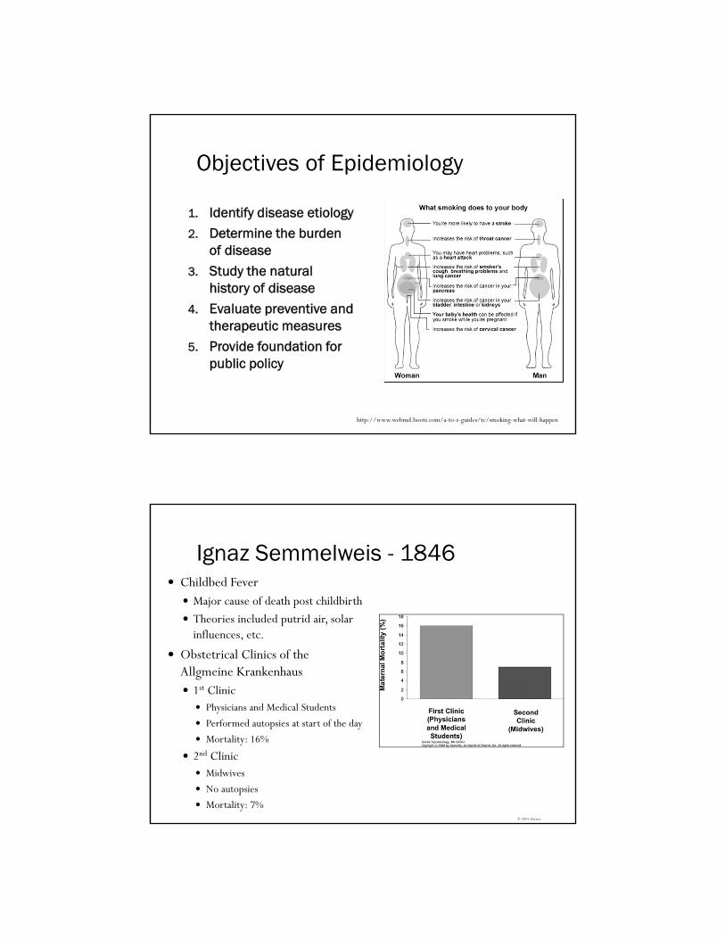
Objectives of Epidemiology
1. Identify disease etiology2. Determine the burden
of disease3. Study the natural
history of disease4. Evaluate preventive and
therapeutic measures5. Provide foundation for
public policy
http://www.webmd.boots.com/a-to-z-guides/tc/smoking-what-will-happen
© 2005 Elsevier
Ignaz Semmelweis - 1846 Childbed Fever Major cause of death post childbirth Theories included putrid air, solar
influences, etc.
Obstetrical Clinics of the Allgmeine Krankenhaus 1st Clinic Physicians and Medical Students
Performed autopsies at start of the day
Mortality: 16%
2nd Clinic Midwives
No autopsies
Mortality: 7%

Suggested transmission of disease from cadavers to women
Noted a colleague died from similar infection after being punctured during an autopsy
Implemented policy that physicians and students wash hands and scrub nails after autopsy, before contact with patients:
Edward Jenner - 1796 Smallpox 400,000 people died per year in
Europe Devastating when introduced to
Americas (biological warfare) Case fatality rate of 40-60%
Variolation and vaccination Originally infected healthy
individuals with material from smallpox patients.
Jenner noted that dairy maids, who were exposed to cowpox, did not develop smallpox.

Smallpox Eradication 1967
~15 million cases per year ~2 million deaths WHO starts efforts to eradicate
smallpox 1980
WHO certifies that smallpox has been eradicated
Last natural case in 1977 Last US vaccinations in 1972
2001 Increased concern about smallpox
and bioterrorism 2014
Small pox found in NIH storage refrigerator
John Snow- 1854 Cholera Severe bacterial infection Miasmatic theory of
disease
London in the 1800s Multiple cholera
pandemics 1831-1854 1949 John Snow published
that cholera was caused by water

“Father of Modern Epidemiology” Combined field work with statistical methods to examine water
sources used by people with cholera.
Broad Street Pump Collected records on 83 deaths
Noted unexpected non-cases
Grand Experiment Multiple companies supplied same
Neighborhoods
Noted that the Lambeth Company
moved intake to a less polluted source
John Snow’s Map
http://scienceblogs.com/significantfigures/index.php/2013/03/11/200-years-of-dr-john-snow-a-significant-figure-in-the-world-of-water/
http://www.youtube.com/watch?v=Pq32LB8j2K8

Richard Doll and Bradford Hill- 1952 Smoking and lung cancer 1920s health care workers noted
that many lung cancer patients also smoked
Incidence of lung cancer in men over 45 rose 6 fold from 1930 to 1945
Cars or other industrial changes.
Experimental design Case-control study Looked at hospital patients with and
without cancer.
Cohort study Prospectively followed >40,000
physicians
BMJ 2004;328:1519

US Lung Cancer Trends
Descriptive and Analytic Epidemiology

Descriptive Epidemiology Includes activities related to characterizing the
distribution of diseases within a population
Analytical Epidemiology Concerns activities related to identifying possible causes
for the occurrence of diseases
Descriptive vs. Analytical Epidemiology
Objectives of Descriptive Epidemiology
To evaluate trends in health and disease and allow comparisons among countries and subgroups within countries
To provide a basis for planning, provision and evaluation of services
To identify problems to be studied by analytic methods and to test hypotheses related to those problems
PERSON
PLACE
TIME
Think of this as the standard dimensions used to track the occurrence of a disease.

Some Definitions Endemic
Habitual presence of a disease in a given area
Usual prevalence of disease within such an area
Epidemic Occurrence in a community or
region of a group of illnesses of similar nature in excess of normal expectancy.
Derived from common or propagated source.
Often called “outbreak” Pandemic
Epidemic over a wide geographic area.
Key Measures in Epidemiology
Morbidity Measures Mortality Measures
Incidence (new cases) Cumulative incidence
(proportion) Incidence rate (new cases
per unit time)
Prevalence (Existing cases) Existing cases Point prevalence
(proportion) Period prevalence
Mortality rate (number of deaths per unit time)
Cumulative mortality (proportion)
Case-fatality rate (proportion of subjects with disease that die from that disease)
Proportionate mortality (proportion of people who die, who died from a specific disease- be careful when using this measure)
The denominator is a key part of measures in epidemiology.

Goal in Analytical Epidemiology Test a hypothesis about relationship between exposure(s) and
disease(s)
Consider Internal Validity Ideal: Free from bias in design, implement, analyze and interpretation Reality: We need to address biases
Consider External Validity Ideal: Generalizable Reality: Applies to study population, infer more broadly
Study Designs for Analytical Epidemiology

Randomized Trials RCTs Randomized Clinical Trials Randomized Control Trials
Often used for studies of treatment/drugs in relation to prognosis
Can also be used in other settings, including studies of risk and prevention
Key elements: Study population is defined Study population is randomly
assigned to two (or more) study “arms”
Outcomes are compared for the different arms
© 2005 Elsevier
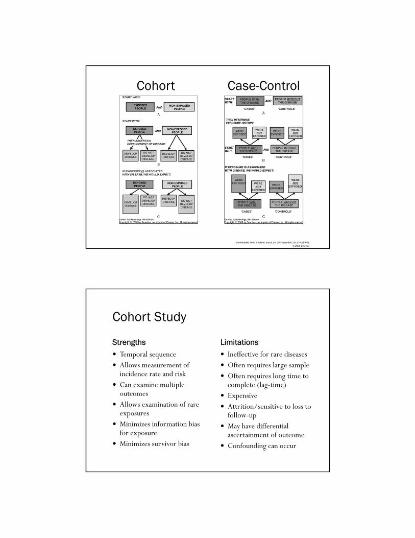
Cohort and Case-Control Studies Observational study designs used in epidemiology Consider strengths, limitations and sources of bias Cohort Study Steps: Define cohort, take baseline measurements and exposure
status, ascertain outcome information, compare incidence in exposed and unexposed
Can be prospective or retrospective
Case-Control Study Steps: Identify cases, identify/select controls, collect exposure
history prior to disase onset, compare odds of exposure in cases to odds in controls
Key step is identifying an appropriate control group
Downloaded from: StudentConsult (on 29 September 2013 04:59 PM)
© 2005 Elsevier
Cohort Case-Control
Cohort Study
Strengths Limitations Temporal sequence Allows measurement of
incidence rate and risk Can examine multiple
outcomes Allows examination of rare
exposures Minimizes information bias
for exposure Minimizes survivor bias
Ineffective for rare diseases Often requires large sample Often requires long time to
complete (lag-time) Expensive Attrition/sensitive to loss to
follow-up May have differential
ascertainment of outcome Confounding can occur
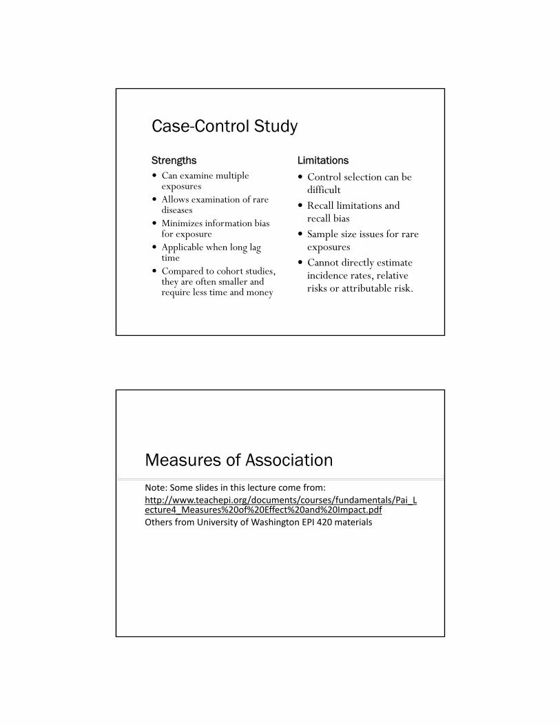
Case-Control Study
Strengths Limitations Can examine multiple
exposures Allows examination of rare
diseases Minimizes information bias
for exposure Applicable when long lag
time Compared to cohort studies,
they are often smaller and require less time and money
Control selection can be difficult
Recall limitations and recall bias
Sample size issues for rare exposures
Cannot directly estimate incidence rates, relative risks or attributable risk.
Measures of AssociationNote: Some slides in this lecture come from:http://www.teachepi.org/documents/courses/fundamentals/Pai_Lecture4_Measures%20of%20Effect%20and%20Impact.pdfOthers from University of Washington EPI 420 materials

Main Measures of Association
Relative Riskmeasure of the relative probability of developing disease based on exposure status
Attributable Riskmeasure of the amount of excess disease incidence attributed to the exposure of interest
Odds Ratiomeasure of the relative odds of exposure based on disease status (can approximate the RR)
The 2x2 Table For Count Data

Relative Risk (RR) For Count Data Used in Randomized trials
Cohort studies
Based on cumulative incidence measure
AKA: Risk Ratio
If no association RR=1
Disease
c+ddc‐
a+bba+
Total‐+Exposure
c/(c+d)
a/(a+b) =
(Incidence of Disease in Unexposed)
(Incidence of Disease in Exposed) RR =
Attributable Risk (AR) for Count Data
Used in Randomized trials and Cohort studies
AKA: Risk Difference*
Difference in risk between exposed and unexposed
If no association AR=0
a/(a+b) ‐ c/(c+d) = Incidence(exposed) – Incidence(unexposed) AR =
Disease
c+ddc‐
a+bba+
Total‐+Exposure
* Note: Some argue that you should use the term risk difference when testing for association, and only use “Attributable Risk” for when you have established causality.

Odds Ratio (OR) for Count Data Used primarily in Case Control
Studies (also in Cohort)
AKA: Relative Odds
Good estimate of RR
If no association OR=1
b*c
a*d=
b/d
a/c=
(Odds of Exposure among Controls)
(Odds of Exposure among Cases) OR =
Disease
c+ddc‐
a+bba+
Total‐+Exposure
What are Odds? Odds: Ratio of ways an event can occur to ways the event can
not occur. Odds of 1:1 indicate both options are easily likely. When rolling dice, probability of getting a 2 is 1/6 Odds of getting a 2 is 1:5.
Used in epidemiology, because of situations where we calculate odds ratios Case-control studies Logistic regression
If P=probability of event, then odds=
If P is very small, 1-P≈1 and odds=

Odds Ratio in Cohort Study and Case-Control Study Reduce to Same Calculation
Odds Ratio Estimates Relative Risk When Disease is Rare The OR will be a good
estimate of the RR if the outcome is rare.
If the outcome is common, and association is positive, then the OR will overestimate the RR
This overestimation can be quite large for common outcomes.

Confidence Intervals and p-values Presentation so far has focused on point estimates
Gives information on magnitude of association
Statistical software will also provide estimate of confidence intervals and p-values
Important to consider precision and statistical significance, along with estimate of magnitude of association.
Bias, Confounding, and Causal Inference

Association and Causality An exposure and outcome are
associated if there is a differential distribution: Incidence of outcome differs
for exposed and unexposed group; or
Prevalence of exposure differs between cases and controls
An exposure is causal for the outcome if the presence (or absence) of the exposure directly or indirectly influences whether the outcome occurs.
2
Phillips, C.V. 2003. Epidemiology. 14(4):459‐466.
Sources of Bias in Epidemiology
What we are trying to measure
What we actually measure
Bias = Systematic error in the design, conduct or analysis of a study that results in a mistaken estimate of an exposure’s effect on the
risk of disease
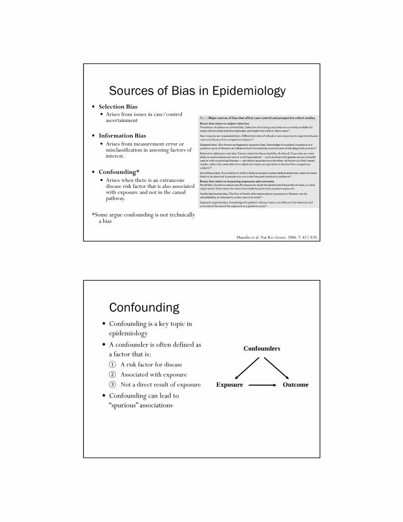
Sources of Bias in Epidemiology
Manolio et al. Nat Rev Genet. 2006. 7: 812-820.
Selection Bias Arises from issues in case/control
ascertainment
Information Bias Arises from measurement error or
misclassification in assessing factors of interest.
Confounding* Arises when there is an extraneous
disease risk factor that is also associated with exposure and not in the causal pathway.
*Some argue confounding is not technically a bias
Confounding Confounding is a key topic in
epidemiology
A confounder is often defined as a factor that is:① A risk factor for disease② Associated with exposure③ Not a direct result of exposure
Confounding can lead to “spurious” associations
Exposure Outcome
Confounders

Example of Confounding Birth order and Down
syndrome Birth order is associated with
Down syndrome, later order children with higher risk Maternal age is associated
with birth order Maternal age is associated
with Down Syndrome
Stratifying on maternal age, there is no longer evidence of an association between birth order and Down syndrome
Approaches to Handling Confounding
In Design of Study In Analysis of Data Randomization
Restriction
Matching Group Matching Individual Matching
Standardization
Adjustment
Stratification

Guidelines for Judging Whether an Association is Causal
Temporal relationship (exposure should proceed outcome) Strength of association (size of odds ratio or relative risk) Dose-response relationship Cessation of exposure leads to reduction in outcome Replication of finding (multiple independent studies) Biological plausibility Consistency with other knowledge Consideration of alternative explanations (ability to rule them out) Specificity of the association
What is Meant by Interaction? Biological Interaction
The interdependent operation of two or more biological causes to produce, prevent or control an effect
Two causes interact on a biological level to cause a disease or outcome
Statistical Interaction The observed joint effects of two factors differs from that expected on the
basis of their independent effects Deviation from additive or multiplicative joint effects
Effect Modification (or Effect Measure Modification) Differences in the effect measure for one factor at different levels of another
factor Example: OR differs for males vs. females; AR differs for pre-menopausal
and post-menopausal women, etc.

Future Directions in Epidemiology
Summary Epidemiology is the study of the distribution and determinants of
health-related states in populations Historic examples demonstrate objectives of epidemiology Study design is a key component of epidemiology Relative risks, risk differences and odds ratios are used to measure
association It is important to consider and address bias in epi studies Selection bias and information bias are two main classes of bias Understanding confounding and effect modification are important
in studies of association Future directions are transforming the field of epidemiology

Definitions of Epidemiology Greek Etymology
Epi - upon, among, on, over Demos- people, populance Logos- study, word, discourse, count
the study of the distribution and determinants of health-related states in specified populations, and the application of this study to control health problems - Last
the study of how disease is distributed in populations and the factors that influence or determine this distribution – Gordis
a branch of medical science that deals with the incidence, distribution, and control of disease in a population – Merriam-Webster
Epidemiology is the study (or the science of the study) of the patterns, causes, and effects of health and disease conditions in defined populations. -Wikipedia

Karen L. Edwards, Ph.D.
Professor
Department of Epidemiology and
Genetic Epidemiology Research Institute
School of Medicine
University of California, IrvineIrvine, CA
Genetic Epidemiology
Introduction
Big Picture Learning Objectives
Familiarity with major study designs used in genetic epidemiology
Familiarity with major issues associated with each approach
Aware of software and web resources used in genetic epidemiology

Course Learning Goals/Objectives
• Define genetic epidemiology
• Describe the fundamental concepts critical to genetic epidemiology
• Describe the major study designs used in genetic epidemiology
• Be able to collect family health information and draw a pedigree using a software program
• Be familiar with resources and current technology used in genetic epidemiology
•Be able to read and discuss the relevant literature
Lecture Outline
• Introduction to Genetic Epidemiology
• Define genetic epidemiology
• Terms and concepts important in genetic
epidemiologyhttp://www.genome.gov/Glossary/http://www.cdc.gov/excite/library/glossary.htm
• Overview of study designs
• Collecting family history information and pedigree
drawing

Genetic Epidemiology
Goals To discover and characterize genetic
susceptibility to health and disease in human populations
To identify interactions between genetic and environmental factors
Use family based studies and studies of unrelated individuals
Apply principals of epidemiology, biostatistics and genetics/genome science
Rapidly evolving field
Percent of Obese (BMI > 30) in U.S. Adults
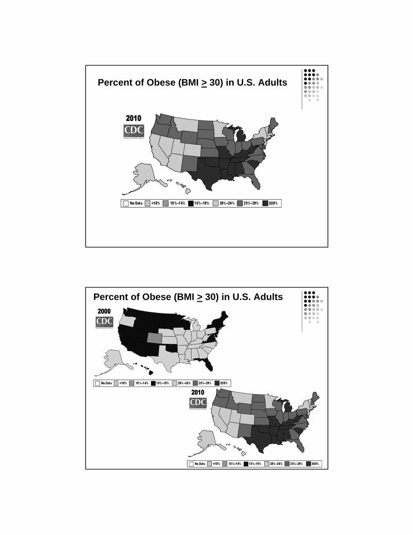
Percent of Obese (BMI > 30) in U.S. Adults
Percent of Obese (BMI > 30) in U.S. Adults

Genetic Epidemiology
Exposure Disease/Outcome
Genotype Phenotype
Phenotype and Genotype
Phenotype and Genotype are the key components in genetic epidemiologic studies
Phenotype (trait) – observed characteristics that are usually the focus of a genetic epidemiologic study
Not always a direct reflection of genotypes
Examples: Blood pressure, body weight, cholesterol level, eye color, heart disease, diabetes, Parkinson’s disease, cancer, longevity
Quantitative vs. qualitative (discrete) trait


Chromosomes, DNA, Genes Chromosomes are made up of DNA and are long strands of “genes”
Humans have about 20,000 genes in their genome
Genes have both coding (exon), noncoding (intron) and regions upstream that affect expression (promoter region)
Promoter region – a sequence of DNA found near beginning of a gene and needed to turn a gene on or off
Exons – contain stretches of DNA that code for proteins
Introns come in between the exons – intervening sequences, do not code for proteins
Genes control growth, development, health and disease
Genes are turned on and off in different patterns and at different stages of development = gene regulation
Genotype The unique genetic information of an individual
Each gene has its own specific location on the chromosome
Genes come in pairs, one version of each gene is inherited from your
mother and one from your father (allele)
Variations in the underlying DNA can result in differences between
individuals, and may underlie a specific phenotype
Different ways of measuring the genotype and alleles
Single nucleotide polymorphism – most SNPs are not themselves functional, but
mark the functional variations that affect disease risk
Sequencing is now common
Factors that affect the expression of the gene (such as environment)
are also important to consider (Gene x environment (GxE))

Genotype Each person inherits 1 chromosome from their biologic
father and one from their biologic mother
23 pairs of chromosomes (a total of 46 chromosomes)
22 of the pairs look the same in males and females
The sex chromosomes differ in males (X, Y) and females (X, X)
Genotype – the unique genetic information from an individual
The genetic contribution to the phenotype
Genotype can refer to a collection of genes or the two alleles of a particular gene
Humans have about 20,000 genes
A pair of chromosomes
Body weight gene (alleles b and B)
Genetic Markers – known locations
b
B

Allele frequencies vary across populations
Humans on the move. Worldwide genetic variation at a neutral marker. Allele frequencies of one randomly chosen microsatellite marker reveal common alleles shared in all populations and the gradual and arbitrary differences in allele frequencies across geographic regions. Populations shown in this example are Yoruba and Bantu (Africa); French, Russians, Palestinians, and Pakistani Brahui(Eurasia); Han Chinese, Japanese, and Yakut (East Asia); New Guineans (Oceania); and Maya and Karitianans (America). From King and Motulsky (2002), Science, 298: 2342-2344.
Identifying genetic effects: Overview

Question Approach
Is there evidence for genetic influences on a quantitative trait? Commingling
Is there familial aggregation? Family Study
Is the familial aggregation caused by genetic factors? Twin Study
Is there a major gene? Is it dominant or recessive ? Segregation Study
Where is this major gene in the human genome? Linkage Analysis
Is there linkage with DNA markers under a specific genetic model?
A. Parametric Approach
Is there an increased allele sharing for affected relatives (sib pairs) or for relatives with similar phenotype
B. Allele Sharing Approach(sib-pair analyses)
Where is the exact location of this gene and which polymorphism is associated with disease?
Association Study (population and family)
Approaches to understanding genetic influences: Overview of Genetic Epidemiologic Studies
Most human traits have a skewed distribution –which could be consistent with a genetic effect
Body weight as our example
Body weight (lbs)
of US Adults
60020050 400
100
500
250
10
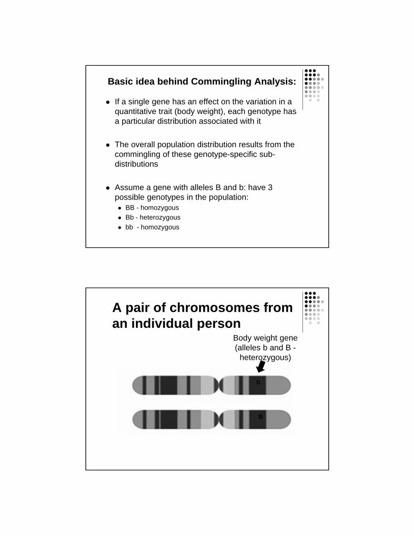
Basic idea behind Commingling Analysis:
If a single gene has an effect on the variation in a quantitative trait (body weight), each genotype has a particular distribution associated with it
The overall population distribution results from the commingling of these genotype-specific sub-distributions
Assume a gene with alleles B and b: have 3 possible genotypes in the population: BB - homozygous
Bb - heterozygous
bb - homozygous
A pair of chromosomes from an individual person
Body weight gene (alleles b and B -
heterozygous)
b
B

Is the frequency distribution of body weight consistent with the influence of a gene with either dominant or recessive effects?
Body Weight
BB, Bb bb
Commingling Analysis Summary:
Why is it used: To provide preliminaryevidence for a single gene that influences a quantitative trait (e.g. body weight, blood pressure, cholesterol level, blood glucose level).
A statistical modeling approach that does not measure the genotype, but assumes genetic principals in the model
Unrelated individuals – faster and easier

Question Approach
Is there evidence for genetic influences on a quantitative trait? Commingling
Is there familial aggregation?higher risk in relatives of cases Family Study
Is the familial aggregation caused by genetic factors?MZ twins concordance rate or correlation higher than DZ twins
Twin Study
Is there a major gene? Is it dominant or recessive ? Segregation Study
Where is this major gene in the human genome? Linkage Analysis
Is there a linkage with DNA markers under a specific genetic model?
A. Parametric Approach
Is there increased allele sharing for affected relatives or for relatives with similar phenotype
B. Allele Sharing Approach(sib-pair analyses)
Where is the disease causing gene and which polymorphism is associated with disease?
Association Study (population and family-based)
Overview of Genetic Epidemiologic Study Design
General comments about twin studies One of the first approaches used to evaluate evidence for
genetic influences on traits
Evaluate both genetic and environmental influences on traits
Measure of interest is the heritability of the trait Proportion of total variance in the quantitative trait due to additive
genetic effects
Population specific
Evaluate evidence for genetic influences on different types of traits qualitative traits – diabetes
quantitative traits – blood glucose
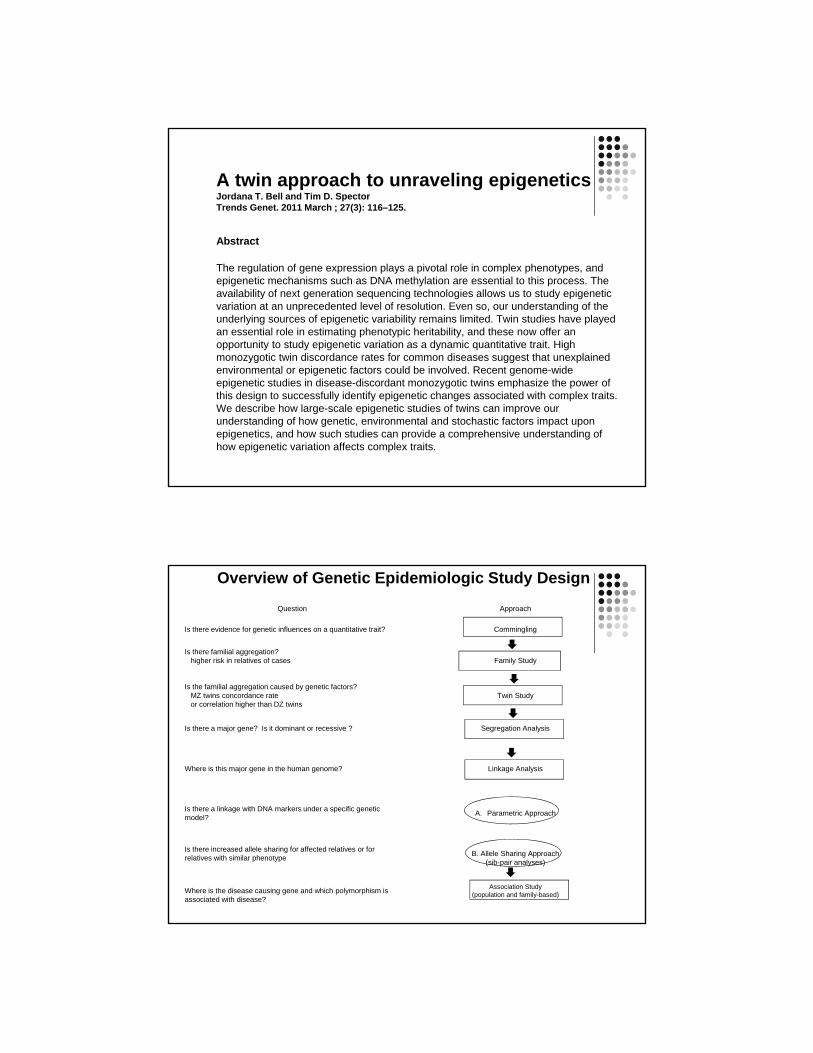
A twin approach to unraveling epigeneticsJordana T. Bell and Tim D. SpectorTrends Genet. 2011 March ; 27(3): 116–125.
Abstract
The regulation of gene expression plays a pivotal role in complex phenotypes, and epigenetic mechanisms such as DNA methylation are essential to this process. The availability of next generation sequencing technologies allows us to study epigenetic variation at an unprecedented level of resolution. Even so, our understanding of the underlying sources of epigenetic variability remains limited. Twin studies have played an essential role in estimating phenotypic heritability, and these now offer an opportunity to study epigenetic variation as a dynamic quantitative trait. High monozygotic twin discordance rates for common diseases suggest that unexplained environmental or epigenetic factors could be involved. Recent genome-wide epigenetic studies in disease-discordant monozygotic twins emphasize the power of this design to successfully identify epigenetic changes associated with complex traits. We describe how large-scale epigenetic studies of twins can improve our understanding of how genetic, environmental and stochastic factors impact upon epigenetics, and how such studies can provide a comprehensive understanding of how epigenetic variation affects complex traits.
Question Approach
Is there evidence for genetic influences on a quantitative trait? Commingling
Is there familial aggregation?higher risk in relatives of cases Family Study
Is the familial aggregation caused by genetic factors?MZ twins concordance rate or correlation higher than DZ twins
Twin Study
Is there a major gene? Is it dominant or recessive ? Segregation Analysis
Where is this major gene in the human genome? Linkage Analysis
Is there a linkage with DNA markers under a specific genetic model?
A. Parametric Approach
Is there increased allele sharing for affected relatives or for relatives with similar phenotype
B. Allele Sharing Approach(sib-pair analyses)
Where is the disease causing gene and which polymorphism is associated with disease?
Association Study (population and family-based)
Overview of Genetic Epidemiologic Study Design

Question Approach
Is there evidence for genetic influences on a quantitative trait? Commingling
Is there familial aggregation?higher risk in relatives of cases Family Study
Is the familial aggregation caused by genetic factors?MZ twins concordance rate or correlation higher than DZ twins
Twin Study
Is there a major gene? Is it dominant or recessive ? Segregation Study
Where is this major gene in the human genome? Linkage Analysis
Is there a linkage with DNA markers under a specific genetic model?
A. Parametric Approach
Is there increased allele sharing for affected relatives or for relatives with similar phenotype
B. Allele Sharing Approach(sib-pair analyses)
Where is the disease causing gene and which polymorphism is associated with disease?
Association Study (population and family-based)
Overview of Genetic Epidemiologic Study Design
Association Studies
Evaluate the association between a particular genetic variant and the trait (disease) in a population
Focuses on unrelated individuals – usually case-control study
Risk is typically estimated by the odds ratio (OR) Compares the frequency of the genetic variant in those with disease to
those without the disease
Measure of the strength of an association OR=1 is no effect, OR>1 is increased risk, OR< is decreased risk
A follow-up or replication study is an important, but challenging aspect of association studies

Summary Genetic Epidemiology - the genetic and environmental
aspects of disease in human populations
Use a variety of study designs to identify and evaluate evidence of genetic effects and impact on disease risk in populations
Integrates epidemiology, genetics, genomics and biostatistics
Collecting Family Data
Genetic Epidemiology

Collecting Family Data
Collecting family data is time consuming and expensive
Need for complete and extended pedigrees
Local relatives vs. all relatives
Collection of phenotype data
Need for accurate description of biologic relationships
Confidentiality and IRB issues in collecting family data

Collecting family data
IRB Issues
Confidentiality of information
Publication of pedigree information, genetic status
Sensitive information
Non-paternity, adoptions, abortions, medical conditions
General approaches to data collection
Proband contact
Individual family members as contacts
Collecting family data Phenotype Information
Survey
Proband onlyPro: quick and inexpensive
Con: lack of knowledge about some relatives
Relatives
Critical information Mother and Father ID for ALL related individuals
Measurements Collecting blood / tissue samples
Physical measurements (height, weight, etc)
Tools for standardized measures (www.phenxtoolkit.org)
PhenX Tool Kit – a catalog of high-priority measures for consideration and inclusion in genetic epi studies


Karen L. Edwards, Ph.D.
Professor
Dept of Epidemiology and
Genetic Epidemiology Research Institute
School of MedicineUniversity of California Irvine
Seattle, WA
Family Studies: Family Health History, Segregation and Linkage
Analysis
Question Approach
Is there evidence for genetic influences on a quantitative trait? Commingling
Is there familial aggregation?higher risk in relatives or higher correlation in relatives
Family Study
Is the familial aggregation caused by genetic factors?MZ twins concordance rate or correlation higher than DZ twins
Twin Study
Is there a major gene? Is it dominant or recessive ? (likelihood of Mendelian models higher than environmental or polygenic model)
Segregation Analysis
Where is this major gene in the human genome? Linkage Analysis
Is there a linkage with DNA markers under a specific genetic model?
A. Parametric Approach
Is there an increased allele sharing for affected relatives (sib pairs) or for relatives with similar phenotype
B. Allele Sharing Approach(sib-pair analyses)
Where is the disease causing gene and which polymorphism is associated with disease?
Association Study (population and family-based)
Overview of Genetic Epidemiologic Study Design

Family Health History: Application to public health
Advantages:• Reflects multiple genetic, environmental, behavioral factors and interactions
• No genetic test can do this
• Family history is a predictor of most diseases (diabetes, cancers, CVD)
• Effective (public health) interventions exist for many of these diseases• Quitting smoking, maintaining ideal body weight, diet, exercise
• Overcomes one of the most important barriers - getting people interested in
learning and talking about their health
Goal: Use family history information to motivate behavior change and promote a
healthy lifestyle for primary prevention of disease• More personalized health messages that “ fit within pre-existing beliefs about
current health status, possible causes and risk factors, course of the disease, magnitude of and potential consequences of the risk, and ways to reduce the risk” See Claassen et al. BMC Public Health 2010, 10:248
Genetic Epidemiology
Segregation Analysis
Complex Segregation Analysis (CSA)
A modeling approach used to determine whether there is evidence for a single gene that underlies a trait or disease
Also provides information on mode of inheritance
Dominant, Recessive or Codominant
General method for evaluating the transmission of a trait within pedigrees
Mendelian transmission
CSA, cont
Information from CSA is useful in model based (parametric) linkage methods
LOD method linkage analysis depends on the specification of a reasonable model, including an approximation of the mode of inheritance Assumes the existence of a Mendelian trait
The goal
To test for compatibility with Mendelianexpectations by estimating parameters for a range of genetic models
CSA can provide the statistical evidence for Mendelian control of a trait or disease
As with all methods so far, this evidence can be used to support a genetic cause of the disease, but is not definitive
Simultaneously considers major locus, polygenic and environmental effects
The Approach
A variety of models are fit to the family data and compared using a likelihood ratio test (for nested models)
The null hypothesis is that the data DO fit with some model of inheritance (genetic or not)- a "goodness of fit" approach

The Models The models are formed by estimating and
restricting a specified set of parameters
The most general model, where all parameters are estimated
Single locus models with no polygenic inheritance and differing modes of inheritance
Polygenic model, with no single locus effect
Mixed model, both single gene and polygenic components
Nongenetic model or "environmental model"
Parameters: single locus component
Means (u) for each subdistribution
Variance of each subdistribution
Allele frequencies
Transmission probabilities - should conform to
Mendelian expectations
t1 = P(AA parents transmits A allele to offspring) = 1.0
t2= P(Aa parents transmits A allele to offspring) = 0.5
t3 = P(aa parents transmits A allele to offspring) = 0.0

Parameters : Polygenic component
Heritability (h2)
proportion of variance due to additive genetic effects
Not a single major gene
Can reflect “residual genetic effects” not accounted for by a single major locus
Sometimes referred to as multifactorial component
Model Testing
Hypothesis testing for nested models using the LRT (likelihood ratio test)
LRT = -2 [In L(reduced model) - In L(full model)]
LRT is distributed as a chi square with the degrees of freedom (df) equal to the difference in the number of estimated parameters
The likelihood of each model is proportional to the probability of the data, given the model and family structure

Model testing, cont
To compare non-nested models
use the AIC to compare (not test) models to support a particular model over another
AIC= -2(ln likelihood) + 2(number of estimated parameters)
Calculate the AIC for each competing model and select the one with the smallest AIC as being the most parsimonious
Interpretation: Inferring A Major Gene
To infer a major gene
reject nongenetic models
accept a major gene model (single or mixed model)
should always test transmission probabilities in CSA of quantitative traits to safeguard against false inference of a major gene

Ascertainment Correction
Ideal probands would be newly diagnosed, population based (incident) cases
Should correct for ascertainment unless pedigrees (probands) are selected from a random, population based sample
Correction for ascertainment is not straightforward and is not usually done
Estimators for population parameters (allele frequency and heritabilty) will be most affected
Review Table

Other Issues to Consider
Nonpaternity seems to have little effect on the ability to select models
Can adjust for covariate effects
Can also consider adjusting for other known genetic factors affecting your trait of interest
Important Limitations in CSA
Implicit assumption of etiologic homogeneity
Power is difficult to estimate as there is no single nongenetic alternative model, but instead a range of competing models
Sample size Larger extended kindreds with several generations
are generally better than small nuclear families
generally requires a large amount of data, with more complex models requiring more data

Summary of CSA
Does not require genotype data
Can be time consuming to complete analyses
Information from CSA is useful for a variety of reasons
Preliminary data, estimates for linkage analyses, choice of phenotype
Assumes the existence of a Mendeliantrait
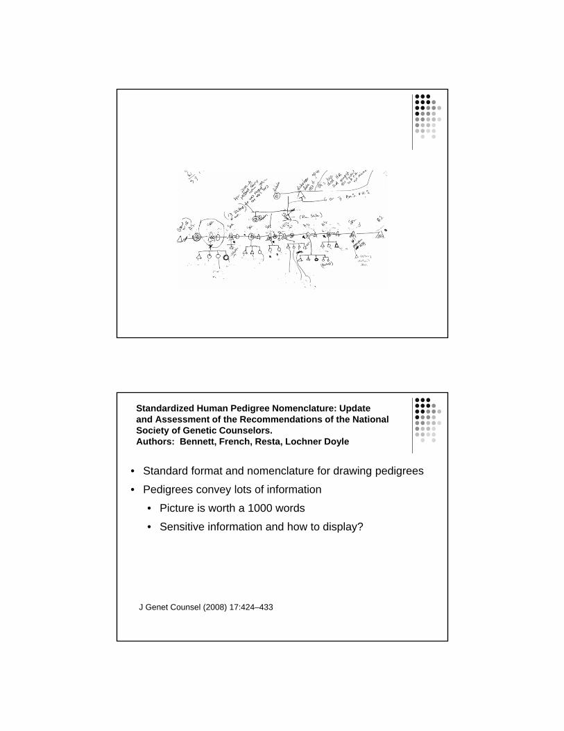
Standardized Human Pedigree Nomenclature: Updateand Assessment of the Recommendations of the NationalSociety of Genetic Counselors. Authors: Bennett, French, Resta, Lochner Doyle
• Standard format and nomenclature for drawing pedigrees
• Pedigrees convey lots of information
• Picture is worth a 1000 words
• Sensitive information and how to display?
J Genet Counsel (2008) 17:424–433

Bennett article - some key points
• A medical pedigree is a graphic presentation of a family’s health history and genetic relationships
• A pivotal tool in the practice of medical genetics / genetic epi research
• Interpreting a pedigree should be a standard competency of all health professionals
• Pedigrees should not contain information about which a subject had no prior knowledge.
• a person who had presymptomatic or susceptibility genetic testing through research should not find out about increased or decreased disease risk status from a publication
In Class Exercise: Pedigree Drawing
Let me start with my great-great grandparents: Jim and Ann Flight.
They had two children: Kathy, and Gerry.
Kathy died in a car accident along with her father Jim.
Gerry married Kate Doe.
Kate and Gerry had one child, Kathy
Kathy Flight married David Dewey and they had my dad, Bob. My dad took his mother’s
maiden name because David had an affair with someone named Maggie Braun.
After Jim’s death, Ann married Paul Wright. Ann and Paul had one child: Tom Wright.
Tom Wright married Kaisa Stone.
Tom and Kaisa had one daughter: Heather. Heather Wright was wed to Peter Meter and had
one child, Jean. Jean married Bob Flight and they had me Jane Flight.

In Class Exercise: Collecting Family History Information
Think about your own family history- Do you know the vital status of your immediate family members,
what about more distant relatives?
- Do you know the DOB and DOD for your immediate family members,
what about more distant relatives?
- What health conditions run in your family?
- Do you know age or date of onset?
- How confident are you in this information?
Draw your pedigree, indicating as much of the following as possible
- vital status, health conditions, age at onset or death
Genetic Epidemiology
Linkage Analysis

Linkage Analysis, overview
Linkage Location of genetic loci sufficiently close together on a
chromosome that they do not segregate independently
linkage is a property of loci (not alleles), and evaluation involves all alleles at the marker locus
the specific alleles segregating in one family may differ from alleles at the same locus segregating in a different family
Linkage vs. Association
Linkage Cosegregation of a disease or trait with a specific
chromosomal region in multiple families
Genetic linkage is the tendency of two loci to be inherited together (e.g. loci are on the same chromosome)
Property of two loci (genes or locations)
Association Presence of a disease or trait with a specific allele in a
gene or marker (in unrelated subjects) – probably due to linkage disequilibrium
Linkage Analysis –background
The aim of linkage analysis is to infer the relative position of two or more loci Examining patterns of allele sharing or cosegregation
of marker and disease in relatives
The location of one locus is known (the marker), the other is unknown (the disease causing gene)
Alleles of loci on the same chromosome can violate Mendels’s law of independent assortment (linkage)
Evidence of linkage between a known marker and a putative gene for a disorder is the ultimate statistical evidence for a genetic component in disease etiology
General Approaches to Linkage Analysis Genome Wide Scan
Isolate a gene solely on the basis of it's chromosomal location, without regard to it's biochemical function.
This is often referred to as the "positional genetic" approach (i.e. genome screens are often referred to positional cloning)
Candidate gene approach Select candidate genes based on their function or other
known properties

Required data for family studies
At least pairs of related individuals
Accurate pedigree structure / biological relationships Nuclear family vs. extended kindred
Phenotype data – quantitative or categorical
Genotype data Location of markers (marker map)
Genetic Markers
A genotype (measurable "trait" ) that is genetically determined, can be accurately classified, has a simple, unequivocal pattern of inheritance (and polymorphic).
Types of genetic markers Polymorphic markers – lots of alleles / variation Variable number of tandem repeats (VNTR) Microsatellites, (e.g. CA repeats), very polymorphic
Single nucleotide polymorphisms (SNP's) - 2 allele markers, very common
Sequence data – exome or whole genome

Statistical Analysis: LOD based Linkage Analysis
Involves comparison of likelihoods of observing the segregation pattern of 2 loci under specific models, including Under the null hypothesis of no linkage Independent assortment – loci recombine as if on
different chromosomes
Alternative hypotheses of linkage differ in the extent of crossing over (i.e. different
values of recombination events)
LOD Score
LOD score = log (base 10) of the odds of linkage vs. no linkage (not an odds ratio!) LOD score > 3, supports linkage, corresponds
to a genome-wide type 1 error rate of 0.05 (depends on number of markers tested)
LOD score < -2, used to exclude a
chromosomal region
Exclusion mapping
add LOD scores from all families to obtain LOD score for your sample Assumes families are independent
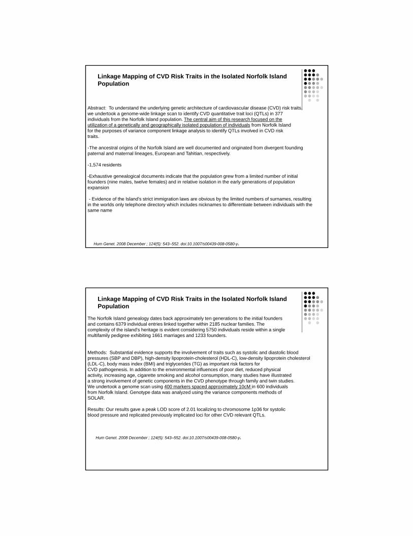
Linkage Mapping of CVD Risk Traits in the Isolated Norfolk IslandPopulation
Hum Genet. 2008 December ; 124(5): 543–552. doi:10.1007/s00439-008-0580-y.
Abstract: To understand the underlying genetic architecture of cardiovascular disease (CVD) risk traits, we undertook a genome-wide linkage scan to identify CVD quantitative trait loci (QTLs) in 377individuals from the Norfolk Island population. The central aim of this research focused on theutilization of a genetically and geographically isolated population of individuals from Norfolk Islandfor the purposes of variance component linkage analysis to identify QTLs involved in CVD risktraits.
-The ancestral origins of the Norfolk Island are well documented and originated from divergent founding paternal and maternal lineages, European and Tahitian, respectively.
-1,574 residents
-Exhaustive genealogical documents indicate that the population grew from a limited number of initial founders (nine males, twelve females) and in relative isolation in the early generations of population expansion
- Evidence of the Island's strict immigration laws are obvious by the limited numbers of surnames, resulting in the worlds only telephone directory which includes nicknames to differentiate between individuals with the same name
Linkage Mapping of CVD Risk Traits in the Isolated Norfolk IslandPopulation
Hum Genet. 2008 December ; 124(5): 543–552. doi:10.1007/s00439-008-0580-y.
The Norfolk Island genealogy dates back approximately ten generations to the initial foundersand contains 6379 individual entries linked together within 2185 nuclear families. Thecomplexity of the island's heritage is evident considering 5750 individuals reside within a singlemultifamily pedigree exhibiting 1661 marriages and 1233 founders.
Methods: Substantial evidence supports the involvement of traits such as systolic and diastolic bloodpressures (SBP and DBP), high-density lipoprotein-cholesterol (HDL-C), low-density lipoprotein cholesterol(LDL-C), body mass index (BMI) and triglycerides (TG) as important risk factors forCVD pathogenesis. In addition to the environmental influences of poor diet, reduced physicalactivity, increasing age, cigarette smoking and alcohol consumption, many studies have illustrateda strong involvement of genetic components in the CVD phenotype through family and twin studies.We undertook a genome scan using 400 markers spaced approximately 10cM in 600 individualsfrom Norfolk Island. Genotype data was analyzed using the variance components methods ofSOLAR.
Results: Our results gave a peak LOD score of 2.01 localizing to chromosome 1p36 for systolicblood pressure and replicated previously implicated loci for other CVD relevant QTLs.

Sib-Pair Linkage Analysis
Sib pairs are generally easier to collect, tend to be more closely matched for age and environment than other relative pairs
Qualitative trait: under linkage, Affected relative pairs should share alleles IBD (inherited from a common ancestor within the pedigree), more often than expected under Mendelian expectations
Quantitative trait: relative pairs should show a correlation between the magnitude of their phenotypic difference and the number of alleles shared IBD
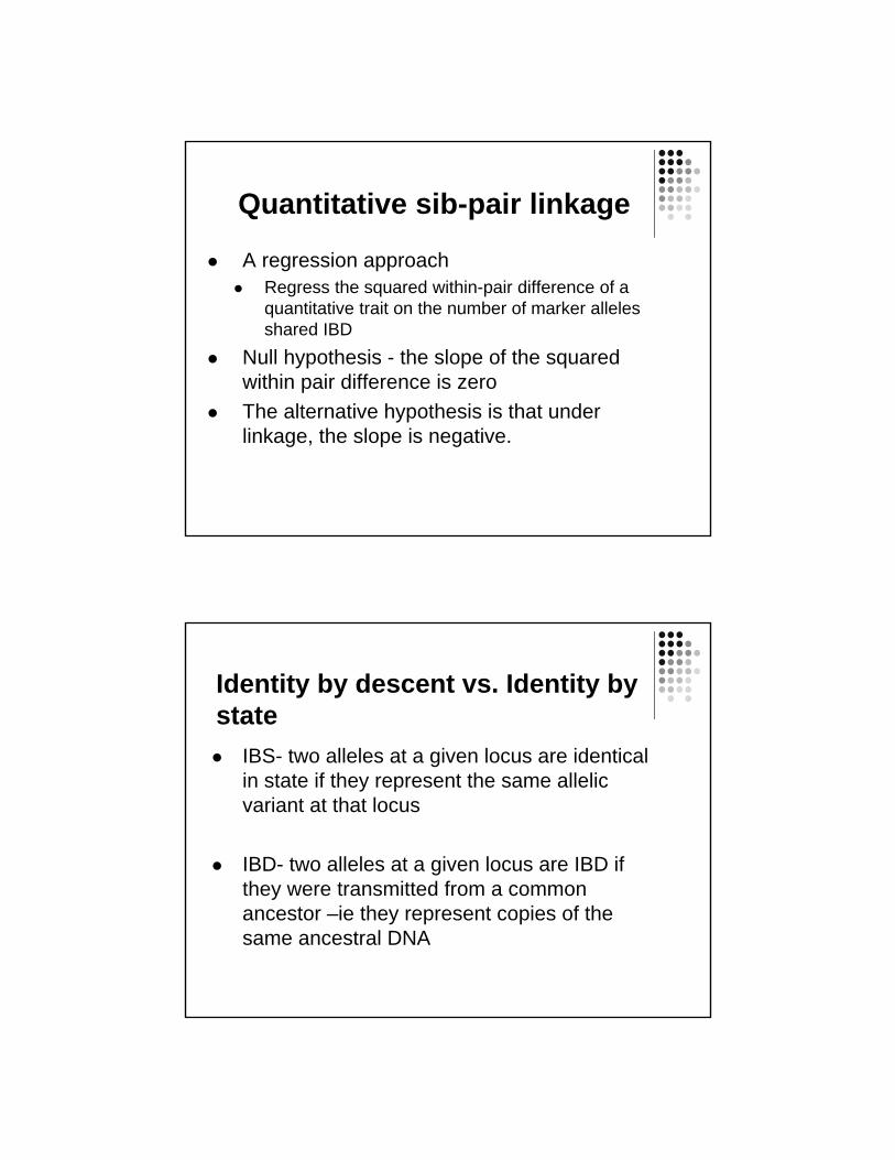
Quantitative sib-pair linkage
A regression approach Regress the squared within-pair difference of a
quantitative trait on the number of marker alleles shared IBD
Null hypothesis - the slope of the squared within pair difference is zero
The alternative hypothesis is that under linkage, the slope is negative.
Identity by descent vs. Identity by state
IBS- two alleles at a given locus are identical in state if they represent the same allelic variant at that locus
IBD- two alleles at a given locus are IBD if they were transmitted from a common ancestor –ie they represent copies of the same ancestral DNA
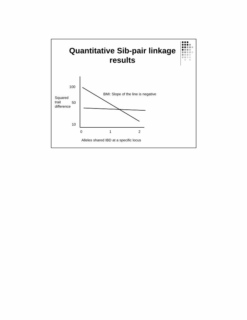
Quantitative Sib-pair linkage results
Alleles shared IBD at a specific locus
0 1 2
Squared trait difference
100
10
50
BMI: Slope of the line is negative

Linkage Disequilibrium
Outline
• Linkage disequilibrium (LD)– Definition of linkage disequilibrium
– Importance of disequilibrium
– Measures of disequilibrium
• SNP selection– Public resources
– Tag SNP selection programs
• Imputation

Definitions
• Allele– Different versions of DNA sequence
at a given location
• Genotype– The two alleles in an individual at a
given locus
• Haplotype– A series of alleles along a single
chromosome
• Diplotype– a set of haplotype pairs in an
individual
SNP1: C and T SNP2: C and A
C C C A
T C T A
SNP1: rs3822050 and SNP2: rs10517002
SNP1: C/C, C/T or T/TSNP2: C/C, C/A or A/A
SNP1 SNP2 SNP1 SNP2
C C C C
C C C A
C C T C
T C T A
Linkage Disequilibrium: Two loci that are in linkage disequilibrium are inherited together more often than would be expected by chance.
Zondervan & Cardon, 2004
Systematic studies of common genetic variants are facilitated by the fact that individuals who carry a particular SNP allele at one site often predictably carry specific alleles at other nearby variant sites. This correlation is known as linkage disequilibrium
The international HapMap consortium, 2005
Linkage Disequilibrium refers to the nonindependence of alleles at different sites. Pritchard and Przeworski 2001
What is Linkage Disequilibrium?

C A C C
T C T A
SNP1 SNP2 SNP1 SNP2
SNP1: C/TSNP2: C/A
C A C C
T C T A
SNP1 SNP2 SNP1 SNP2
SNP1: C/TSNP2: C/A
Linkage Equilibrium
Linkage Disequilibrium
haplotype frequencies in population match what is expected based on allele frequenciesExample: frequency of C-A haplotype equals frequency of C allele at SNP 1 * frequency of A allele at SNP 2
haplotype frequencies in population differ from what is expected based on allele frequencies
It is a Matter of Scale
"Nothing in biology makes sense except in the light of evolution”-Theodosius Dobzhansky, 1973

Current Haplotypes Arose from Ancient Mutation Events
1. Ancestral state has no variation at either SNP position.
2. Mutation leads to first SNP
3. Asecond mutation leads to second SNP
4. Recombination or recurrent mutation needed for all four haplotypes
C A
T A
T C
C A
C AT A
C A
T AT C
C C
T A
C A
T C
Haplotypes
The International HapMap Consortium. Nature | Vol 437 | 27Octobe

Focus on Pairwise LD
A a
B pAB paB pB
b pAb pab pb
pA pa
A B
a b
a B
A b
If loci are independent, then we expect pAB= pA* pB
pAb= pA* pb
pAB= pA* pB
pAB= pA* pB
Measuring LD for pairs of sites‐ D
One important measure of LD is
DAB = pAB – pApB
Notice that D=0 if and only the two sites are independent
A disadvantage of D is that the range of possible values depends greatly on the marginal allele frequencies.
A a
B pAB paB pB
b pAb pab pb
pA pa
A B
a b
a B
A b

Measuring LD for pairs of sites‐ D’
Lewontin (1964) proposed an adjusted
statistic that has range [-1, 1]:
D’ = D/max(D), where max(D) is dependent on the marginal allele frequencies
If DAB>0: D’AB = DAB/(min(PaPB, PAPb))
If DAB<0: D’AB = DAB/(min(PAPB,PaPb))
A a
B pAB paB pB
b pAb pab pb
pA pa
Properties of D’
• D’ favored in medical genetics
– D’=0 implies independence
– |D’|<1 implies that there has been recombination between the two sites in the history of the sample (or recurrent mutation)
– |D’=1| implies “complete LD”
• No historic recombination
• Neither site has experienced recurrent mutation or gene conversion
• Genotypes not perfectly correlated (unequal allele frequency)
• D’ inflated in smaller samples

Measuring LD for pairs of sites‐ r2
Along with D’, the other most widely
used statistic is r2:
r2 = DAB2 / (pA*pB*pa*pb)
r2 has range [0,1]. Its value is 1 if
just 2 of the 4 haplotypes are present.
r2 is intimately connected to the power of association mapping [Pritchard & Przeworski 2001]
A a
B pAB paB pB
b pAb pab pb
pA pa
Properties of r2
• r2 favored in population genetics– r2 =0 implies independence
– r2 =1 implies “perfect LD”• Marker loci have identical allele frequencies
• Genotype is perfectly correlated
– Related to power if (N2=N1/r2)
• where N1 is sample size needed for directly genotyped SNP, N2 is sample size needed to test tagged SNP and r2 is the LD between the directly genotyped SNP and the tagged SNP).
• Assume need 1,000 for directly genotyped SNP, examples of sample size needed for tagged SNPs, depending on r2
– r2=1.0, N1= N2=1,000
– r2=0.2, N2 = 1,000/0.2 = 5,000

What factors affect LD?
• Mutation
• Historical recombination
• Natural selection
• Founder effects
• Migration
• Random drift
• Population admixture
LD over time
• Recombination assorts SNPs on haplotypes.
• Under assumption of random mating and a large population, LD will break down over time.

Applications of LD
• LD is the sine qua non of genetic association studies:– We are interested in testing for an association between disease status and causal mutations
– If all polymorphisms were independent at the population level, association studies would have to examine every one of them.
– Instead we can test a subset and get information on all of them.
• LD is also used in studies of human history, natural selection and the biology of recombination
Genotype at one site can predict genotype at another site
Proportion of sites are correlated
LD Across a Gene
SNP Selection
• We use information about allele frequencies and LD across the genome to make informed choices as to which variants to genotype
– Identify SNPs in region of interest
– Interested in minimal set of SNPs needed to capture variation in region.
Identify variation for your region
• Option 1: sequence individuals in your sample for the entire gene/region of interest
• Option 2: sequence a subset of individuals to identify variation in your region
• Option 3: Use public databases to identify known variation in your region

SNP Database Resources
• NCBI SNP Database, dbSNP– http://www.ncbi.nlm.nih.gov/SNP/
• International HapMap Project– http://www.hapmap.org/
• NHLBI Program for Genomic Applications (http://www.nhlbi.nih.gov/resources/pga/)– SeattleSNPs (http://pga.mbt.washington.edu/)
– InnateImmunity (http://innateimmunity.net/)
• 1,000 genomes project– http://www.1000genomes.org
• Exome variant server (EVS)– http://evs.gs.washington.edu/EVS/
Tag SNPs
– tagSNPs • SNPs are selected based on their pair wise ability to predict genotype of untyped SNPs
• Based on an r2 concept of LD structure• Example program: LDSelect
– haplotype‐tagging SNPs (htSNPs) • SNPs are selected to optimize resolution of existing haplotypes
• Based on a D’ concept of LD structure• Example program: Haploview, HaploBlockfinder
– Multi‐marker tagSNPs• Use tagSNP concept, but extend past pair wise LD• Example program: tagger

Tag SNPs – using r2 information
Think-Pair-Share Exercise:
Which SNPs are in high LD?How many SNPs would you
need to genotype to effectively capture the
variation across the region?
A/T1
G/A2
G/C3
T/C4
G/C5
A/C6
AATT
GC
CG
GC
CG
TCCC
ACCC
GGAA
After Carlson et al. (2004) AJHG 74:106
Tag SNPs – using r2 information
Tags:
Test for association:
A/T1
G/A2
G/C3
T/C4
G/C5
A/C6
AATT
GC
CG
GC
CG
TCCC
ACCC
GGAA
After Carlson et al. (2004) AJHG 74:106

European-AmericansCRP
African-AmericansCRP
Tag SNPs are Population Specific
Thousand Genomes and GVS Tutorial

Limitations of tag SNPs
• Ultimately, we are interested in identifying common polymorphisms that are causally associated with disease risk, we cannot determine if signal is from the tagSNP or from a correlated SNP.
• What happens if your tagSNP fails in the genotyping/QC stage?
Imputation
• We also use LD information to impute genotype information.
• Common example is in genome‐wide association studies.
– Example: SNPs on a GWAS chip can be used to infer information on all variants in HapMap and 1000 genomes data
• Recent literature focuses on appropriate reference populations (see for example Eur J Hum Genet. 2015 Jul;23(7):975‐83. )

Imputation with family data
Imputation with Population Data
Nature Reviews Genetics 11, 499-511 (July 2010)
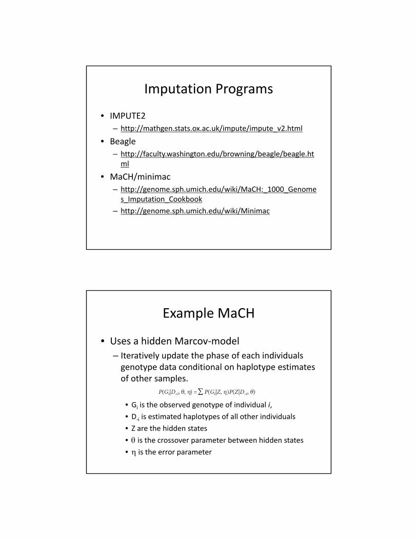
Imputation Programs
• IMPUTE2
– http://mathgen.stats.ox.ac.uk/impute/impute_v2.html
• Beagle
– http://faculty.washington.edu/browning/beagle/beagle.html
• MaCH/minimac
– http://genome.sph.umich.edu/wiki/MaCH:_1000_Genomes_Imputation_Cookbook
– http://genome.sph.umich.edu/wiki/Minimac
Example MaCH
• Uses a hidden Marcov‐model
– Iteratively update the phase of each individuals genotype data conditional on haplotype estimates of other samples.
• Gi is the observed genotype of individual i,
• D‐i is estimated haplotypes of all other individuals
• Z are the hidden states
• is the crossover parameter between hidden states
• is the error parameter

Imputation Output
• A “best guess” genotype (i.e. TT)• Probability of each genotype (i.e. pr(TT), pr(TA), pr(AA))
• A “dosage”. If T is 0 and A is 1, then people are on a scale from 0 to 2 (where 0=TT, 1=TA and 2=AA). • dosage=pr(TA)+2*pr(TT)
• A quality score (typically an “information” or r2 measure) that captures the uncertainty in the imputation.
Summary
• Linkage disequilibrium (LD) refers to the nonindependence of alleles at different sites in the genome
• LD is shaped by population genetic forces• We exploit LD information in genetic epidemiology– Selecting tagSNPs for association studies– Imputation in GWAS studies
• LD complicates interpretation of association studies

Tag SNPs – using r2 information
Tags:
SNP 1SNP 3SNP 6
3 in total
Test for association:
SNP 1 captures 1 & 2SNP 3 captures 3 & 5SNP 6 captures 4 & 6
A/T1
G/A2
G/C3
T/C4
G/C5
A/C6
high r2 high r2 high r2
AATT
GC
CG
GC
CG
TCCC
ACCC
GGAA
After Carlson et al. (2004) AJHG 74:106
Tags:
SNP 1SNP 3
2 in total
Test for association:
SNP 1 captures 1+2SNP 3 captures 3+5
SNP 1 and 3 in combo also captures 4 and 6
Picking tag SNPs using multimarker r2
AATT
GC
CG
GC
CG
TCCC
ACCC
GC
CG
TCCC
GGAA
GGAA
A/T1
G/A2
G/C3
T/C4
G/C5
A/C6
http://www.broad.mit.edu/mpg/tagger