SinksMathew Evans, Daniel Jacob,

Bill Bloss, Dwayne Heard, Mike Pilling

• Sinks are just as important as sources for working out emissions!

1. NOx N2O5 hydrolysis

2. OH Comparison with direct observations

N2O5 hydrolysis

• ‘Ultimate’ NOx sinks dominated byOH + NO2 + M HNO3 (historically

interesting)

N2O5 + aerosol HNO3

• Roughly 50% from eachOH+NO2 dominates in summer

N2O5 + aerosol dominates in winter

N2O5 + aerosol

• Rate defined by the ‘reaction probability’

• Fraction of molecules that hit aerosol surface that react

• For the stratosphere 0.1

• But is this true for the troposphere– Different types of aerosols– Warmer and wetter

Rumblings of discontent

• Tie et al., [2003] found N2O5<0.04 gave a better simulation of NOx concentrations during TOPSE

• Photochemical box model analyses of observed NOx/HNO3 ratios in the upper troposphere suggested that N2O5 is much less than 0.1 [McKeen et al., 1997; Schultz et al., 2000]

New literature

• Kane et al., 2001 - Sulfate – RH– JPL

• Hallquist et al., 2003 - Sulfate - temp– Tony Cox’s group in Cambridge

• Thornton et al., 2003 - Organics - RH– Jon Abbatt’s group at U Torontio

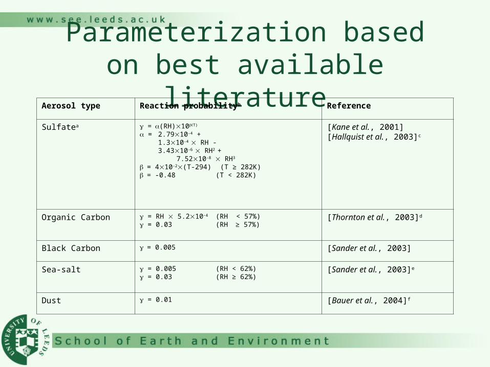
Parameterization based on best available literature

Aerosol type Reaction probabilityb Reference

Sulfatea =(RH)10T)

= 2.7910-4 + 1.310-4 RH -3.4310-6 RH2 +

7.5210-8 RH3 = 410-2(T-294) (T ≥ 282K)= -0.48 (T < 282K)

[Kane et al., 2001] [Hallquist et al., 2003]c

Organic Carbon = RH 5.210-4 (RH < 57%) = 0.03 (RH ≥ 57%)

[Thornton et al., 2003]d

Black Carbon = 0.005 [Sander et al., 2003]

Sea-salt = 0.005 (RH < 62%) = 0.03 (RH ≥ 62%)

[Sander et al., 2003]e

Dust = 0.01 [Bauer et al., 2004]f

What s do we get?

• Much lower than 0.1• Dry low values• Higher at the surface

What is the impact on composition?Lower N2O5

higher N2O5

250%

higher NO330%

higher NOx 7%

Higher NOx

higher O3

7%

Higher NOx higher OH

8%

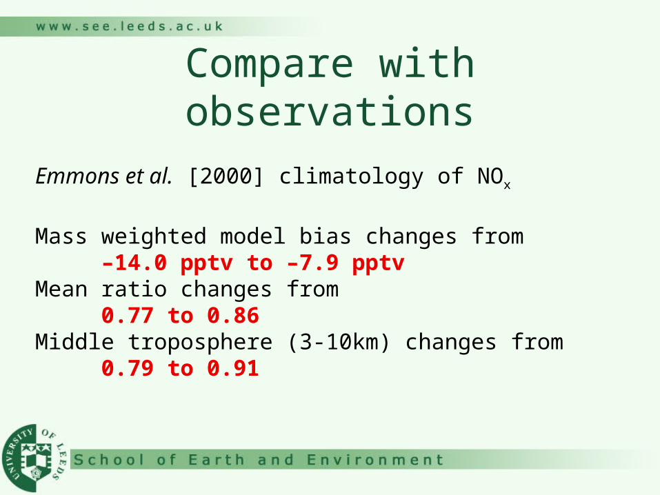
Compare with observations

Emmons et al. [2000] climatology of NOx

Mass weighted model bias changes from –14.0 pptv to –7.9 pptv

Mean ratio changes from 0.77 to 0.86

Middle troposphere (3-10km) changes from 0.79 to 0.91

Compare with observations

Logan [1998] Ozonesonde climatologyMass weighted model bias

-2.9 ppbv to -1.4 ppbv Mean ratio changes from

0.94 to 0.99. Ox (odd oxygen) budget

Chemical production increases 7% 3900 Tg O3 yr-1 to 4180 Tg O3 yr-1

Compare with observations

Global annual mean tropospheric OH 0.99106 cm-3 to 1.08106 cm-3 8% increase.

Both values are consistent with the current constraints on global mean OH concentrations based on methyl-chloroform observations:

1.07 (+0.09 -0.17) 106 cm-3 [Krol et al., 1998] 1.16 0.17 106 cm-3 [Spivakovsky et al., 2000] 0.94 0.13 106 cm-3 [Prinn et al., 2001]

Conclusions

• Aerosol reaction of N2O5 is very important for the atmosphere

• Previous estimates have been too high

• New laboratory data allows a better constraint

• Sorting out old problems although not ‘sexy’ is important

Future improvements

• Assumed (NH4)2SO4

• But model ‘knows’ the degree of neutralization in the aerosol

• There is a inhibiting effect of nitrate on uptake

• Future lab studies – dust?

• Is the ‘cost benefit’ worth improving it?

A ‘cheeky’ bottom-up evaluation of global mean

OH

Global mean OH

How do they calculate global mean OH

• Methyl chloroform made by a few large chemical companies

• Sources are known (nearly)

• Can measure concentrations across the globe

• Then invert to get the sink

Bottom up approach

• Can directly observe OH

• But lifetime of OH is ~ 1s

• So measurements at one site don’t tell you much about global concentrations

• Is this true?

• Can we get a ‘bottom up’ global OH distribution?

NAMBLEX, EASE ’97, SOAPEX

• OH measured by the FAGE group in chemistry

• Time series of OH

• Can we use this to provide information about global OH

• ‘Couple’ global atmospheric chemistry model and the observations

Observed vs Modelled OH

Mac

e H

ead

- Ir

elan

d

More useful comparisonMeasured mean is 1.8 × 106 cm-3, Modelled mean is 2.3 × 106 cm-3

Ratio of 1.56 ± 1.62.

The statistical distribution of the ratio is not normal and so more appropriate metrics such as the median (1.13) or the geometric mean (1.13 +1.44

-0.64 ),

The model simulates 30% of the linear variability of OH (as defined by the R2).

The uncertainty in the observations (13%) suggests that the model systematically overestimates the measured OH concentrations.

Other HOx components

Over a yearSmoothed mean OH from

modelSampled for the

NAMBLEX campaign

Sampled for the EASE ‘97 campaign

Observed Campaign means

Other places

Cap

e G

rim

- A

ust

ralia

So what have we learnt?

• Mace Head we tend to over estimate

• Cape Grim doesn’t seem so bad

• Can we combine this information and the model to get a global number?

• Very Cheeky!

What do we get?All

106 cm-3

A Priori

OH

(Model)

Compare

Observed OH

A Posteri

OH

Prinn et al.

OH

NH 1.12 -19% 0.91 0.90 ± 0.20

SH 1.02 +1% 1.03 0.99 ± 0.20

Global 1.07 -9 % 0.97 0.95

What does this mean

• Very, very lucky!!!!

• The FAGE OH and the MCF inversions seem consistent

• Model transfer seems to work

• Uncertainties suggest it could have gone the other way

Can we do this better?

• Include more data– Aircraft campaign– Surface sites– Ships

Availability of data

How do we incorporate this?

• Principal components of the GEOS-CHEM tracers

• Redefine the temporal and spatial space in terms of different components

• ‘Optimal estimate’ of global mean OH

• Don’t know if this will work

Component 1

Component 2

Component 3

Component 4

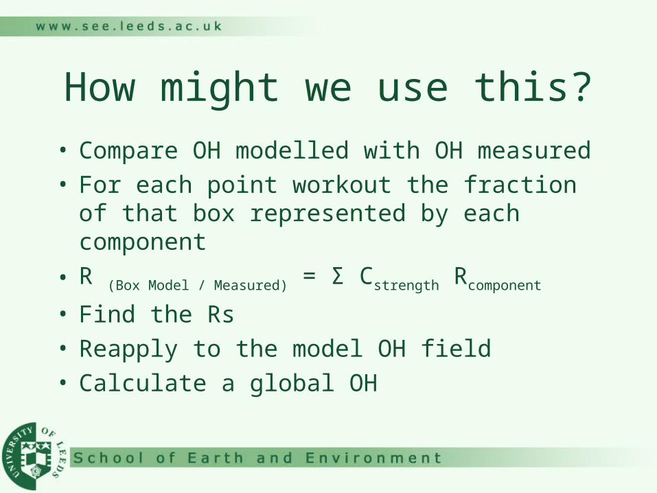
How might we use this?• Compare OH modelled with OH measured• For each point workout the fraction of that box

represented by each component

• R (Box Model / Measured) = Σ Cstrength Rcomponent

• Find the Rs• Reapply to the model OH field• Calculate a global OH

Conclusions

• CTM comparison with OH looks pretty good

• We can use this information to constrain the model OH and this gives a reasonable result

• To take this further requires a bit more thought