Single View Reconstruction of Curved Surfaces

Mukta Prasad, Andrew Zisserman

University of Oxford, U.K.

http://www.robots.ox.ac.uk/∼{mukta,vgg}

Andrew Fitzgibbon

Microsoft Research, Cambridge, U.K.

http://www.research.microsoft.com/∼awf

Abstract

Recent advances in single-view reconstruction (SVR)

have been in modelling power (curved 2.5D surfaces) and

automation (automatic photo pop-up). We extend SVR

along both of these directions. We increase modelling

power in several ways: (i) We represent general 3D sur-

faces, rather than 2.5D Monge patches; (ii) We describe a

closed-form method to reconstruct a smooth surface from

its image apparent contour, including multilocal singulari-

ties (“kidney-bean” self-occlusions); (iii) We show how to

incorporate user-specified data such as surface normals,

interpolation and approximation constraints; (iv) We show

how this algorithm can be adapted to deal with surfaces of

arbitrary genus. We also show how the modelling process

can be automated for simple object shapes and views, us-

ing a-priori object class information. We demonstrate these

advances on natural images drawn from a number of object

classes.

1. Introduction

The reconstruction of 3D objects from 2D images has

long been of interest to researchers in computer vision and

computer graphics. Our objective in this paper is to recon-

struct a smooth 3D model from a single image, and in par-

ticular to compute a 3D model which projects exactly to the

object outline (or apparent contour) in the image. This is

an instance of single-view reconstruction: the problem of

fitting 3D geometry and a camera projection to a 2D im-

age. We follow two recent strands of research: the mod-

elling of curved 3D surfaces [10, 15] and the automation of

single-view segmentation and modelling using object class

recognition techniques [6].

Horry et al.’s 1997 “Tour into the picture” [7] might be

considered the first SVR system, allowing piecewise planar

reconstructions of paintings and photographs. Subsequent

systems [1, 13] improved the geometric accuracy of SVR—

particularly for scenes with multiple vanishing points or

planes—as well as demonstrating the extraction of (relative)

metric information from uncalibrated pictures, or even re-

Figure 1. Single-view reconstruction of a curved object from its

apparent contour. Our method computes the global optimum of

surface smoothness while exactly matching complex apparent con-

tours arising from multilocal events.

naissance paintings. However, the above systems remained

essentially restricted to planar scenes. In parallel, recon-

struction of special classes of curved surfaces, such as sur-

faces of revolution and straight homogeneous generalized

cylinders [16], was developed by several authors. Utcke

and Zisserman [15] give a recent survey. By specifiying

the local surface normal, height, and surface discontinuities,

relatively complex scenes could be extracted. However the

surface representation was rather limited, being restricted

to 2 1

2D Monge patches. Prasad et al. [10] extended this

scheme to allow the reconstruction of 3D mesh surfaces of

simple topology given simple apparent contour constraints,

and providing all of the contour generator is visible.

Related to this is work on the shape from silhouette prob-

lem. The reconstruction of curved surfaces from the ap-

parent contour was considered by Terzopoulos et al. [14]

in their work on symmetry seeking models. In these tech-

niques, a snake is initialized around the object outline, and

image-based forces latch this snake to the projection of a

parametrized 3D shape. However this and related methods

were iterative, and maintaining a consistent mesh through

the iterations is problematic. More recent level-set tech-

niques [2] greatly reduce the consistency problem, but re-

main iterative solutions, prone to being stuck in local min-

ima.

We focus in this paper on extending the class of linear

solutions, attracted by its global optimality guarantees, and

extend the methods to deal with more complex topologies,

and to deal with the case where the apparent contour dis-

plays discontinuities (see figure 1).

A second recent strand in single-view reconstruction is

automation. Hoiem et al. [6] apply methods from the recent

object recognition literature to learn texture and segmenta-

tion cues for a number of common object classes (e.g. build-

ings, sky, ground plane). These cues yield an approximate

segmentation of the source image which can be refined by

fitting a piecewise-planar 3D model to the scene, resulting

in a “photo pop-up”.

For curved surfaces of the type we shall consider, an im-

portant first first step in fully automating 3D pop-out is ob-

taining the apparent contour. Methods like GrabCut [12]

can segment out an object given user supplied information

about its foreground distribution (e.g. by drawing a bound-

ing box). This is taken a step further in OBJCUT [9] where

models of particular object classes (cows, horses) are learnt

in advance, and no user interaction is required to segment

out objects of learnt classes.

Class-specific 3D reconstruction may also be learned

when a database of 3D models or multi-camera views is

available. Romdhani and Vetter [11] use a linear basis for

the 3D shape and then MAP estimation to instantiate shape

from a single image, while Grauman et al. [3] learn to gen-

erate virtual views from a single silhouette from which a

visual hull can be computed. Our long-term goal is to al-

low photo pop-up for a variety of curved shapes for which

3D models may not be readily available (glass, flowers), so

we prefer to learn an object-specific 2D segmentation and

to combine that with a generic 3D modelling method.

The paper outline is as follows. In section 2 we describe

our closed-form solution to reconstruction from a single-

view silhouette in the presence of multilocal singularities.

In section 4 we show how object-recognition cues can be

used to generate automatic pop-up of curved objects. We

conclude in section 5 with a discussion of our results and

with directions for development of this work.

2. Smooth surface reconstruction subject to ap-

parent contour constraints

In this section we describe the basic framework for ob-

taining a smooth 3D object from an image. The model is ob-

tained by minimizing a surface smoothness objective func-

tion subject to constraints from the apparent contour. We

will describe the method first for a simple view of a surface

with cylindrical topology (see figure 2), and then introduce

the generalizations for other topologies (genus 0,1,2) and

more general viewpoints.

2.1. Surface representation and generation

Following Terzopoulos et al. [14] we use the stan-

dard parametric surface representation, r : [0, 1]2 7→ R3,

since this allows us to model truly 3D freeform sur-

faces. The continuous surface S is denoted as r(u, v) =(x(u, v), y(u, v), z(u, v))⊤. The surface is computed by

minimizing a smoothness objective function (the thin-plate

energy [4] or bending energy)

E(r) =

1∫

0

1∫

0

‖ruu‖2 + 2‖ruv‖

2 + ‖rvv‖2 du dv (1)

subject to the constraint that the surface’s contour genera-

tor projects to the given image contour. To optimize this

we choose a gridded discretization (recently dubbed the ge-

ometry image [5]), representing r by three m × n matrices,

X, Y, Z. When solving for the surface, we shall reshape and

stack these matrices into a single vector g =[

x⊤ y⊤ z⊤]⊤

where lowercase x represents the reshaping of X into a col-

umn vector. Central difference approximations are used for

the first and second derivatives on the surface, and are rep-

resented by appropriate matrix operators [15]. Thus the first

derivative term xu at a point (i, j) is discretely approxi-

mated as

Xu(i, j) = X(i + 1, j) − X(i − 1, j),

ignoring boundary bookkeeping and scaling for the mo-

ment. This is conveniently represented by a constant mn ×mn matrix Cu such that xu = Cux. A similar matrix Cv

computes the central difference with respect to v, and we

term these two matrices the Jacobian operator matrices with

respect to u, v. Similarly the second derivatives are com-

puted using Hessian operator matrices denoted Cuu, Cuv and

Cvv . In terms of these, then, the bending energy (1), can be

expressed in discrete form as a quadratic function of g:

ǫ(x) = x⊤(C⊤uuCuu + 2C⊤uvCuv + C⊤

vvCvv)x (2)

E(g) = ǫ(x) + ǫ(y) + ǫ(z) (3)

= g⊤Cg (4)

where C is 3mn × 3mn square matrix.

In the following subsections we introduce linear con-

straints from the apparent contour of the form Ag = b.

This linearity is important because it leads to a standard

minimization of a quadratic form g⊤Cg subject to linear

constraints. This problem has a unique solution which may

be readily obtained using standard numerical methods.

2.2. The Apparent Contour Constraint

Terminology: The image outline of a smooth surface Sresults from surface points at which the imaging rays are

tangent to the surface [8].

(a) (b) (c)

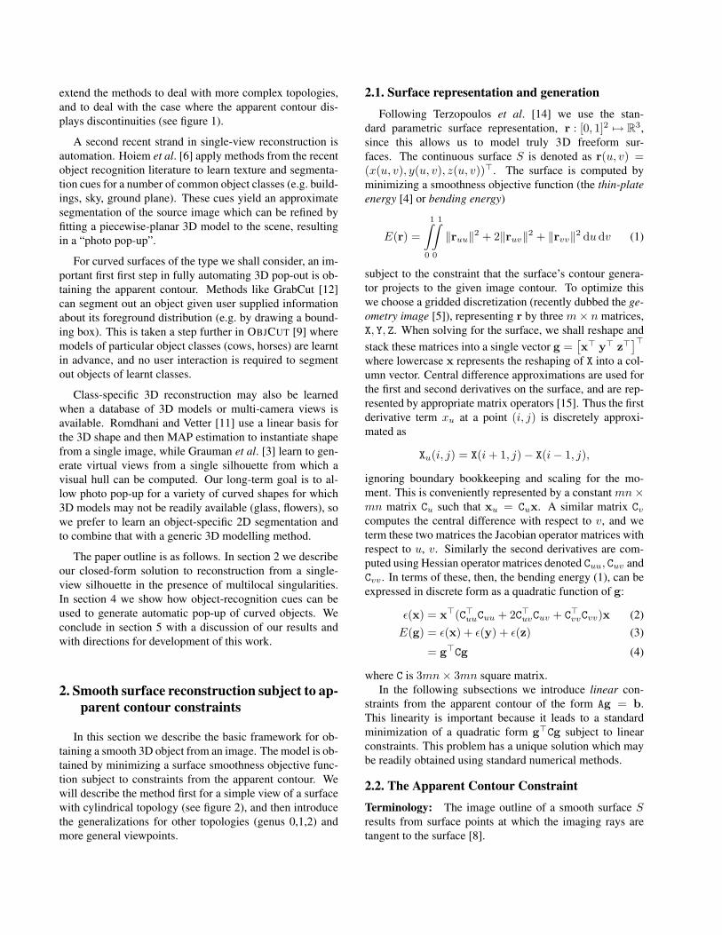
Figure 2. Reconstruction of 3D surface from apparent contour

constraints. (a) The apparent contour is marked on the input im-

age. (b) If optimizing curvature, we are at liberty to place the

contour generator’s domain (see §2.2) anywhere in the parameter

space, providing topological constraints are maintained. In prac-

tice we minimize an approximation to curvature. A reasonably

finely sampled parametrization yields good results, and allows a

global optimum to be found. (c) Reconstructed surface, with con-

tour generator superimposed. Our contribution is to extend this

construction to cases where the CG is not simple.

The contour generator (CG) Γ is the set of points {c (t) |0 ≤ t ≤ 1} on S at which rays from the viewer are tangent

to the surface. The image of the contour generator is called

the apparent contour γ, and is the set of points s which are

the image of c, i.e. γ is the image of Γ. The apparent con-

tour is also called the “outline”, “profile”, or “silhouette”.

The CG is a 3D curve on the surface. If the surface

is viewed in the direction of r from the camera centre, then

the surface appears to fold, or to have a boundary or contour

generator.

The apparent contour constraints can be summed up as:

• The candidate 3D model must project to the 2D ap-

parent contour. We assume orthographic projection,

which is adequate for the approximate models we are

building.

• At the CG, the surface must also be tangent to the

viewing direction.

These important image-based constraints are readily avail-

able.

The CG’s domain is a curve in the (u, v) parameter

space. If that curve is D = {d(t) = (u(t), v(t))|0 ≤ t ≤1} then the CG is c(t) = r(u(t), v(t)). We are given an

image apparent contour γ = {s(t)|0 ≤ t ≤ 1} i.e. γ is

the infinite set of 2D points on the apparent contour and we

are assuming it is parametrized by the same t as the CG. At

each point on the 2D apparent contour, we can compute the

2D unit normal (nx, ny). Under orthographic projection

along Z, the corresponding 3D normal at the CG n, must

have a Z component of zero. Therefore, the 3D normal at

t is given by n(t) = (nx, ny, 0). This means we know the

surface normal at any point on the contour generator, so the

(infinite) set of linear constraints which force the apparent

contour of the 3D surface r to coincide with s are

( 1 0 00 1 0

)r(u(t), v(t)) = s(t) [Projection] (5a)

n(t)⊤ru(u(t), v(t)) = 0 [Normal] (5b)

n(t)⊤rv(u(t), v(t)) = 0 [Normal] (5c)

Prasad et al. [10] observe that there is a freedom in the

parametrization, so that the curve in (u, v) space which

is the pre-image of the contour generator can be chosen.

This means that (u(t), v(t)) in the above constraints are

known points. For the case of a cylinder from a simple

viewpoint, curves of constant u in the (u, v) are chosen as

the domain of the CG—see the vertical bold lines in fig-

ure 2. In particular we choose the uniformly spaced curves

u = ul = 1

4, u = ur = 3

4, to coincide with the CG.

In a discrete setting, each segment of the contour gen-

erator is represented by a set of 2D edgel points, the result

of Canny edge detection and linking. Let us consider just

the left segment, corresponding to u = ul. The 2D curve

is approximately arc-length sampled at n points, giving 2D

points {(sj , tj)}nj=1

, with associated 2D normals (pj , qj).If we let (il, j) in general be the integer grid coordinates

corresponding to parameter space location (ul, v), then we

may write the above constraints in terms of our discretiza-

tion as

X(il, j) = sj j = 1..n (6a)

Y(il, j) = tj j = 1..n (6b)

pjXu(il, j) + qjYu(il, j) = 0 j = 1..n (6c)

pjXv(il, j) + qjYv(il, j) = 0 j = 1..n (6d)

amounting to 4n linear constraints on X and Y (remember-

ing that Xu is linear in X etc). By reshaping matrices appro-

priately, these may be rewritten as a matrix equation of the

form Alg = bl, where Al is of size 4m×mn. We can repeat

this process for the other contour generator segment, giving

constraints Arg = br. Stacking these matrices, and others

we shall see later, into a single large matrix yields the com-

plete set of linear constraints Ag = b. The minimization

of E(g) from (4) above is then standard [15]: our objective

function is quadratic and constraints are linear. This means

that we can formulate a Lagrangian for the problem as

L = g⊤Cg + λ⊤ (Ag − b) (7)

Optimizing this Lagrangian is equivalent to solving the ma-

trix equation given by,

[

C AT

A 0

] [

g

λ

]

=

[

0

b

]

(8)

which is readily achieved using sparse methods.

1

3

42

1

2

3

4

(a) (b) (c) (d)

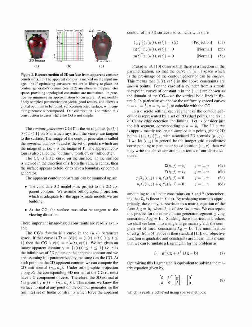
Figure 3. Reconstruction from a complex apparent contour. (a) Input image, with user-selected Canny edge chains. Curve 1 is a

simple segment of the apparent contour. Curves 3 and 4 represent a continuous segment of the apparent contour which corresponds to a

discontinuity in the 3D contour generator. Curve 2 is a crease discontinuity which extends curve 3. (b) These curves may be laid out in

parameter space so as to preserve their incidence relationships. (c,d) Projections of the recovered 3D surface from two views.

2.3. Inflation constraints

The constraints expressed in (5) constrain the x and ycoordinates of the surface only. There are no constraints

imposed on z. Our approximation to curvature in the form

of the bending energy does not couple the z energy to that of

the x and y terms, meaning that contour constraints produce

a surface which projects correctly to the apparent contour

but has z(u, v) = 0 ∀u, v. In order to avoid this trivial

solution we need to “inflate” the surface and flesh it out

into a plausible model. To achieve this, depth constraints

are supplied and the surface is fitted to either interpolate or

approximate these constraints.

An interpolation constraint is of the form

r(uk, vk) = rk (9)

for given (uk, vk, rk), the subscript indicating that there

might be several such constraints. Constraints may also be

supplied on just a single component of a point’s position,

such as its depth, z(uk, vk) = zk. For example, we may

insist that the surface passes through the plane z = 1 at

(u, v) = ( 1

2, 1

2), and the plane z = −1 at (u, v) = (0, 1

2).

Each of these constraints may again be expressed as linear

functions of the surface discretization g.

For the vase in figure 2, the inflation constraints provided

were interpolation constraints which assumed the surface to

be a fronto-parallel surface of revolution. Although this is

a simple strategy, it still pays to use the general framework,

because it guarantees that the contour generator projects

correctly. If the contour generator does not project correctly

(as can happen when simply constructing a surface of rev-

olution from the image contour), texture mapping gathers

pixels from the background, leading to a nasty stain on the

object surface.

The reconstruction, produced by these constraints, ex-

pressed at particular parameter locations, depends on the

(u, v) locations. But for simple surfaces the sensitivity to

choice of (u, v) is generally low, as seen in §3.4 and fig-

ure 6. For more complex surfaces however, or where there

is significant foreshortening, it is useful to supply approx-

imation constraints. Approximation constraints cause the

surface to pass near certain 3D points, for example, by min-

imizing an additional energy term of the form

αk‖r(uk, vk) − rk‖2 (10)

The factor αk controls the extent to which each constraint

should be satisfied. A collection of such constraints may be

represented as the quadratic term ‖Mg − m‖2 (embedded

with α), giving the modified Lagrangian

L = g⊤Cg + ‖Mg − m‖

2+ λ⊤ (Ag − b) (11)

Optimization of this Lagrangian boils down to the slightly

modified matrix equation shown below.

[

C + M⊤M A

⊤

A 0

] [

g

λ

]

=

[

M⊤m

b

]

(12)

As an example of the application of these constraints, the

surface in figure 3 was constrained to approximately meet

the planes z = my ± 1 using the constraints z(0.5, v) ≈mv + 1; z(1.0, v) ≈ mv − 1. The value of m is determined

interactively in order to obtain the best-looking shape.

3. More General Surfaces and Views

In this section we increase the scope of single-view re-

construction in two ways: first, we deal with more com-

plicated viewpoints. These are still generic viewpoints, but

now the apparent contour may terminate (where the view di-

rection is asymptotic) or be self occluded (a bi-local event);

second we generalize the topology, and move from cylin-

ders to spheres, and from genus zero to genus 1 and 2.

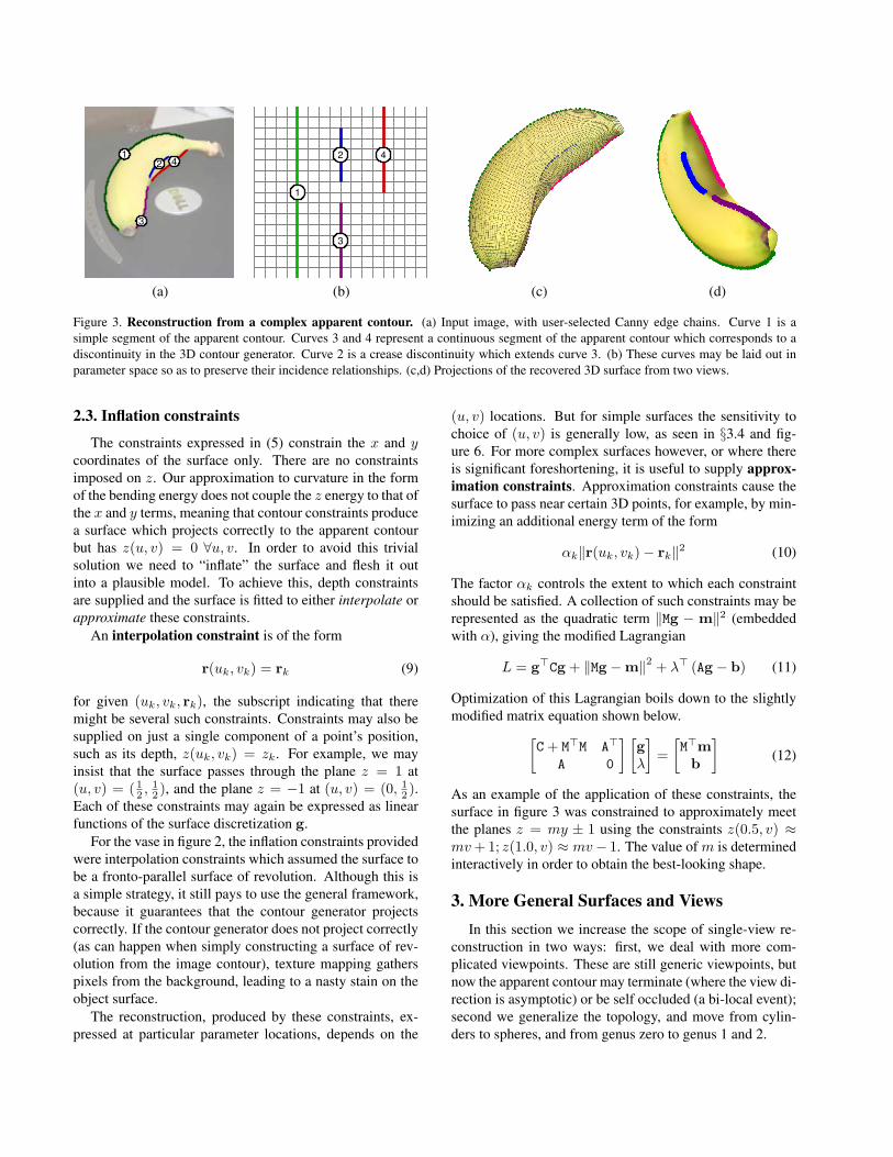
(a) Genus 0 (cylindrical) (b) Genus 0 (spherical) (c) Genus 1 (toroidal) (d) Genus 2 parametrization

Figure 4. Topology. The first row shows the parameter space for each of the topologies listed in the bottom row. The arrow types indicate

which ends of the parameter space must join with each other. The dotted line in column 2 indicates that all points on that parameter line join

at one point. For surfaces of genus > 1, the hole in the surface translates to two holes in the parameter space as shown in column 4. Images

and reconstructions of surfaces of the respective topologies are shown on Rows 2 and 3, with the apparent contour constraint represented

as green and magenta curves.The genus 2 teapot without texture mapping demonstrates the power of the parametrization

(a) (b) (c) (d)

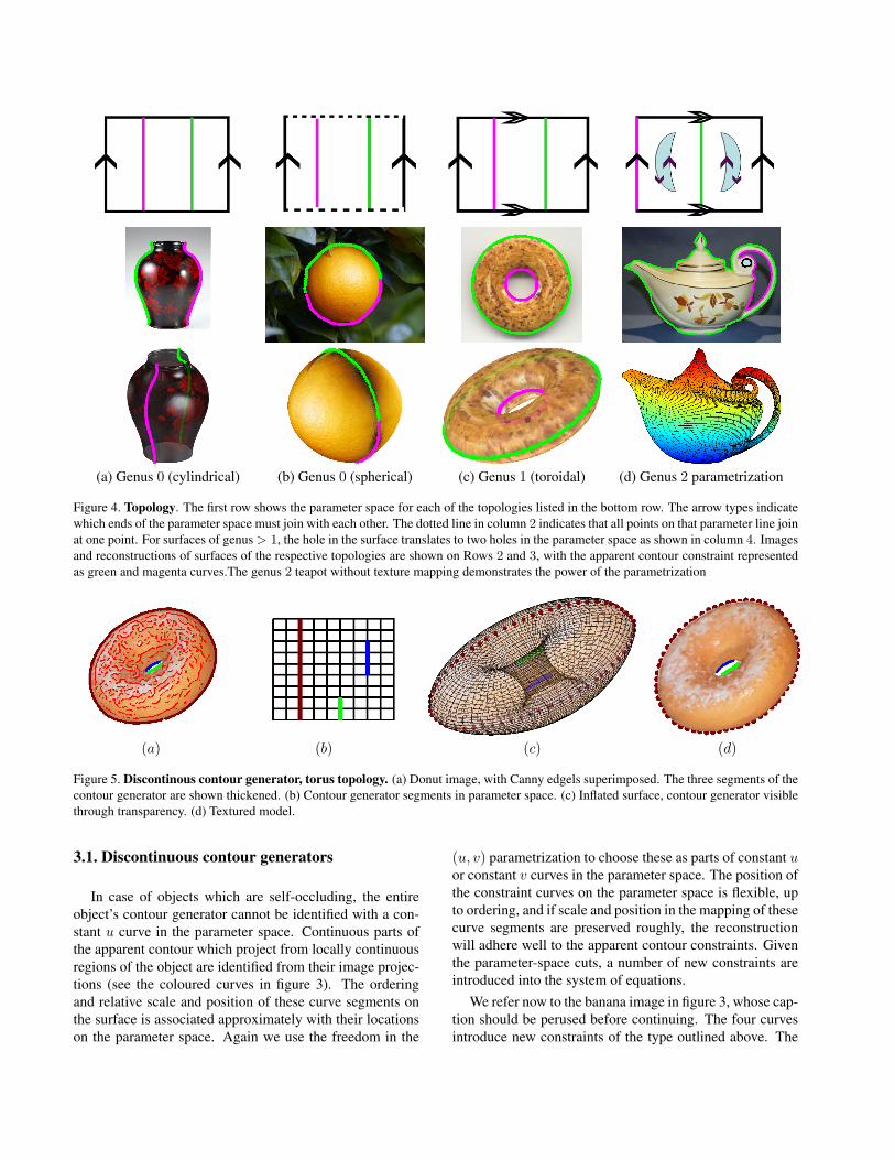
Figure 5. Discontinous contour generator, torus topology. (a) Donut image, with Canny edgels superimposed. The three segments of the

contour generator are shown thickened. (b) Contour generator segments in parameter space. (c) Inflated surface, contour generator visible

through transparency. (d) Textured model.

3.1. Discontinuous contour generators

In case of objects which are self-occluding, the entire

object’s contour generator cannot be identified with a con-

stant u curve in the parameter space. Continuous parts of

the apparent contour which project from locally continuous

regions of the object are identified from their image projec-

tions (see the coloured curves in figure 3). The ordering

and relative scale and position of these curve segments on

the surface is associated approximately with their locations

on the parameter space. Again we use the freedom in the

(u, v) parametrization to choose these as parts of constant uor constant v curves in the parameter space. The position of

the constraint curves on the parameter space is flexible, up

to ordering, and if scale and position in the mapping of these

curve segments are preserved roughly, the reconstruction

will adhere well to the apparent contour constraints. Given

the parameter-space cuts, a number of new constraints are

introduced into the system of equations.

We refer now to the banana image in figure 3, whose cap-

tion should be perused before continuing. The four curves

introduce new constraints of the type outlined above. The

left-hand side of the apparent contour is handled just as

above (6) (note that in this example the CG is non-planar—

this is handled perfectly using the previous machinery).

Curves 4 and 3 are simply segments of contour generator

handled as above, noting that they must not occupy the same

u = constant curve in parameter space because they are

disjoint on the object. Denote curve 3 as extending from

(u3, 0) to (u3, v3), and curve 4 from (u4, v4) to (u4, 1). It

is not important where the curve endpoints are placed in the

v direction, although it uses grid resolution most effectively

if they are placed so that the curves are roughly arc-length

parametrized when re-projected into the image.

Curve 2 is a particular class of curve on a 3D object. Be-

cause it corresponds to a crease discontinuity, it is visible in

the image after it has ceased to be part of the contour gen-

erator. Thus we can identify it, and assign it to the same

u-constant parameter line as curve 3. This creates a more

pleasing parametrization and generates a more plausible 3D

model, in conjunction with crease discontinuity handling

(§3.3).

3.2. Topology

The parametric surface representation allows us to rep-

resent surfaces of different topology and shape. As with the

contour generator, topology can be represented quite read-

ily by various cuttings of the parameter space. Although

somewhat complex, these cuttings need be worked out only

once per topological class. Figure 4 illustrates the various

cases, and we consider some examples to show how these

are implemented in our optimization framework.

For the cylindrical topology of figure 4, the essential

constraint is that points on the u = 0 curve (i.e. the 3D

curve {r(0, v)|0 ≤ v ≤ 1}) are neighbours of points on the

u = 1 curve. In a continuous parametrization, it would be

natural to implement this as a set of incidence constraints

on the surface and its derivatives

r(0, v) = r(1, v) ∀v, (13a)

ru(0, v) = ru(1, v) ∀v, (13b)

ruu(0, v) = ruu(1, v) ∀v, etc. (13c)

which is again linear in r. In a discrete implementation, this

is a waste of 1/m of the parameter space and complicates

bookkeeping. In practice it is simpler to make X(1, j) and

X(m, j) neighbours in the derivative computations by mod-

ifying the Jacobian operator matrix Cu, as well as the appro-

priate second derivative operators. For spherical topology,

these incidence constraints are augmented with the con-

straints that: (i) r(u, 0) = r(0, 0)∀u which is again lin-

ear in r, and is implemented as the 3m linear constraints;

and (ii) rv(u, v) = rv

((

u + 1

2

)

mod 1, v)

∀u; v ∈ {0, 1}.

The torus topology is a straightforward modification of

the cylindrical case. Finally, higher genus surfaces require

somewhat more profligate use of the parameter space. To

make a genus two surface requires that two loops of param-

eter space are identified. In this case, modification of the

derivative operator matrices is not for the faint-hearted, and

recourse to a simple parameter identification as in (13) is

probably the best course of action. One such implemen-

tation of a genus 2 surface can be seen in figure 4. For a

logical choice of the loop and a reasonable resolution, the

precise choice does not greatly affect surface shape.

3.3. Surface creases

One final generalization is to allow the surface to crease.

This means, as with the apparent contour, specifying a curve

in the parameter space (say u = uc), and constraining

points along this curve to project to the image of the crease

as in (5a). The second modification is to E(r): replacing the

bending energy, computed from second derivatives, with a

membrane energy—the sum of squares of first derivatives

across the curve. Considering the contribution to E(r) at a

point (uc, v) on the crease, we replace

‖ruu‖2 + ‖ruv‖

2 + ‖rvv‖2

with

‖ruu‖2 + ‖rv‖

2

so that the term transverse to the curve permits high second

derivatives, allowing the crease to form when E is mini-

mized. This is implemented by augmenting C with first-

derivative terms, and adding weights to control the influ-

ence of each row of C. The energy remains quadratic in the

surface g and a global minimum is easily found.

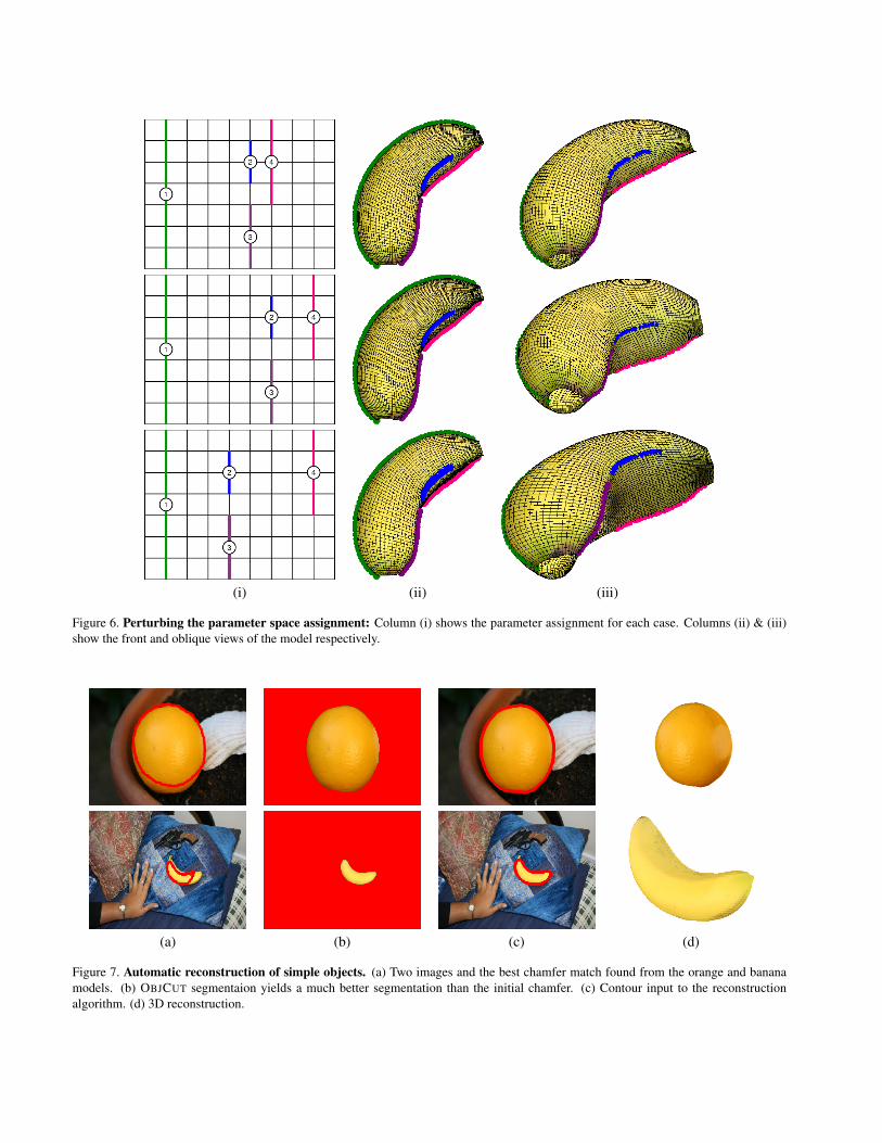
3.4. Sensitivity to parameter assignment

At several points throughout the paper we make special

choices of parameter-space points and curves, remarking

that the precise values chosen will have a minimal effect

on the recovered surface. In theory this is true if the en-

ergy being minimized is invariant to parametrization, for

example surface curvature. In practice we are not minimiz-

ing curvature, merely a proxy for it. This proxy computes

derivatives in the parametric space and does not take actual

3D distances into account. So the parametrization does af-

fect the object shape. We illustrate that this effect is small

by perturbing our assignments in the parameter space by

approximately 20% of their original assignment values for

the banana example. The models produced using identical

inflation are shown in figure 6. Varying the parameter as-

signment results in different but all convincing models. The

sensitivity to perturbation also depends on the object com-

plexity and the availability of constraints. One workaround

is to use derivatives weighted by 3D distances and find the

optimal surface by iteratively fitting and reparametrizing the

surface.

The object shape is closely related to the density of

parametrization. For an object with large variations in

curvature, parametrizing sufficiently densely that the high-

curvature sections are modelled will waste effort in densely

sampling near-planar areas. These questions are among

those addressed by Gu et al.’s “geometry image” work [5].

4. Automation

Complete automation of single view reconstruction for

particular curved surface classes requires a number of steps:

(i) Detect the apparent contour curves—for example by seg-

menting out the object; (ii) identify the contours in the pa-

rameter space; (iii) generate a surface consistent with ap-

parent contours (this may require inflation hints); (iv) tex-

ture map the surface from its image appearance. We have

demonstrated steps (iii) and (iv), we now address step (i):

segmenting out the object automatically.

For segmentation we employ the OBJCUT formulation

of Kumar et al. [9]. In this method, segmentation is treated

as a binary MRF labelling problem. The MRF includes like-

lihoods from the foreground and background colour/texture

distributions, and the segmentation is guided by a pictorial

structure object model (the pictorial structure prior is what

OBJCUT adds to the model over earlier work such as Grab-

Cut [12]). The initial distributions and pictorial structure

are learnt from training images of the object class.

In brief, we use 25 training images for oranges and 30

for bananas. The implementation of OBJCUT is from code

supplied by the authors of [9]. This algorithm is successful

in segmenting many of the images. There are occasional

problems when the initial chamfer match of the pictorial

structure is attracted to erroneous edges.

Figure 7 shows examples of completely automated re-

constructions. These involve segmentation (with OBJCUT)

and the assumption that the views are simple for each class

(so that the apparent contour may be identified with the seg-

mentation boundary). Of course, in the case of an orange,

there are only simple views.

5. Discussion

We have presented several new extensions of recent work

on modelling smooth shapes from their apparent contours.

In particular we have demonstrated the accurate recovery of

a 3D parametric surface with a discontinuous, non-planar

contour generator. Our method results in a system of linear

equations, yielding the globally optimal energy. In addi-

tion, we have shown how the modelling framework can be

extended to deal with complex topologies, again with dis-

continuous contour generators.

The issues discussed in §3.4 must be dealt with. To avoid

the challenges posed by non-linear minimization methods,

we hope to solve these problems with a more realistic en-

ergy and iterative minimization methods.

Finally, the inflation strategy we use is also a by-product

of not minimizing curvature. It is somewhat clumsy and in-

creases the amount of user skill required to make models.

We hope to find ways of better approximating a curvature-

like energy or alternatively, devise a better inflation mecha-

nism to alleviate this difficulty.

References

[1] A. Criminisi, I. Reid, and A. Zisserman. Single view metrol-

ogy. IJCV, 40(2):123–148, Nov 2000.

[2] O. D. Faugeras and R. Keriven. Complete dense stereovision

using level set methods. In Proc. ECCV, pages 379–393,

1998.

[3] K. Grauman, G. Shakhnarovich, and T. Darrell. Virtual vi-

sual hulls: Example-based 3D shape inference from a single

silhouette. In Proc. 2nd Workshop on Statistical Methods in

Video Processing, 2004.

[4] W. E. L. Grimson. From Images to Surfaces: A Computa-

tional Study of the Human Early Visual System. MIT Press,

1981.

[5] X. Gu, S. J. Gortler, and H. Hoppe. Geometry images. In

ACM Trans. Graph., pages 355–361, New York, NY, USA,

2002. ACM Press.

[6] D. Hoiem, A. A. Efros, and M. Hebert. Automatic photo

pop-up. ACM Trans. Graph., 24(3):577–584, 2005.

[7] Y. Horry, K. Anjyo, and K. Arai. Tour into the picture: Using

a spidery mesh interface to make animation from a single

image. In Proc. ACM SIGGRAPH, pages 225–232, 1997.

[8] J. Koenderink. Solid Shape. MIT Press, 1990.

[9] M. Kumar, P. Torr, and A. Zisserman. OBJ CUT. In Proc.

CVPR, pages I: 18–25, 2005.

[10] M. Prasad, A. W. Fitzgibbon, and A. Zisserman. Fast and

controllable 3D modelling from silhouette. In Eurographics,

Short Papers, 2005.

[11] S. Romdhani and T. Vetter. Estimating 3D shape and tex-

ture using pixel intensity, edges, specular highlights, texture

constraints and a prior. In Proc. CVPR, pages II: 986–993,

2005.

[12] C. Rother, V. Kolmogorov, and A. Blake. “GrabCut”: inter-

active foreground extraction using iterated graph cuts. ACM

Trans. Graph., 23(3):309–314, 2004.

[13] P. Sturm and S. J. Maybank. A method for interactive 3D re-

construction of piecewise planar objects from single images.

In Proc. BMVC., 1999.

[14] D. Terzopoulos, A. Witkin, and M. Kass. Symmetry-seeking

models for 3D object reconstruction. Proc. ICCV, pages

269–276, 1987.

[15] L. Zhang, G. Dugas-Phocion, J. Samson, and S. Seitz. Single

view modeling of free-form scenes. In Proc. CVPR, pages

I:990–997, 2001.

(i) (ii) (iii)

Figure 6. Perturbing the parameter space assignment: Column (i) shows the parameter assignment for each case. Columns (ii) & (iii)

show the front and oblique views of the model respectively.

(a) (b) (c) (d)

Figure 7. Automatic reconstruction of simple objects. (a) Two images and the best chamfer match found from the orange and banana

models. (b) OBJCUT segmentaion yields a much better segmentation than the initial chamfer. (c) Contour input to the reconstruction

algorithm. (d) 3D reconstruction.