SINGLE MOLECULE OPTICAL ABSORPTION BY STM AND A NEW ALGORITHM FOR

SOLVING DYNAMICS ON A FREE ENERGY SURFACE

BY

GREGORY EARL SCOTT

DISSERTATION

Submitted in partial fulfillment of the requirements

for the degree of Doctor of Philosophy in Chemistry

in the Graduate College of the

University of Illinois at Urbana-Champaign 2011

Urbana, Illinois

Doctoral Committee:

Professor Martin Gruebele, Chair

Professor Joseph Lyding, Co-Director of Research

Associate Professor Harley Johnson

Professor J. Douglas McDonald

ii

Abstract

The combination of the high spatial resolution of the scanning tunneling microscope (STM) and the

spectral resolution of a laser provides a powerful tool for probing the local optical and electronic

properties of materials. Optical absorption detected by STM offers direct imaging of molecular

absorption well below the diffraction limit that hampers traditional spectroscopic methods. This

technique is used to optically differentiate carbon nanotubes within nanometers of each other and, further,

to resolve local variations in absorption within a single carbon nanotube. Provided from this is direct

imaging of the spatial distribution of exciton generation from an optical absorption event. The

interactions between light and single molecules are shown to be highly wavelength dependent and are

very sensitive to the local electronic environment.

Relating experimental thermodynamic and kinetic data to the dynamics on free energy surfaces can be

cumbersome for all but the most trivial of cases. Many models have been developed to explain a variety

of phenomena, but few methods are appropriate for cases with low kinetic barriers. Those methods that

do fit free energy surfaces with low barriers are typically computationally expensive in multiple

dimensions. A new method is presented for solving dynamics on free energy surfaces based on the

Smoluchowski diffusion equation. Computational cost is saved by reducing the complexity of the surface

through the use of a singular value decomposition basis set. Fitting is performed with a parallelized

genetic algorithm. Free energy surfaces are fitted in up to 2-dimensions for the α3D and PTB1:4W

proteins. The algorithm is further used to create test data for a new method for finding thermodynamic

data from kinetic experiments when thermodynamic experiments are insufficient for probing the stability

of proteins.

iii

Acknowledgements

While most of the experimental work described in this dissertation was performed under vacuum

conditions, my work has not been done in vacuum in the literary sense of the word. I owe a great deal of

thanks to a number of individuals who have cultivated my development as a scientist and educator, many

of whom do not appear on this short page of tribute.

I am extremely grateful for the opportunity to work under the guidance of Professor Martin Gruebele

throughout my time as a graduate student. I could not have asked for a better advisor under which to

grow professionally and personally. Martin is both an excellent researcher and a dedicated educator and I

only hope that I can emulate his leadership style as I being my career in academia. I have also had the

great fortune to learn from Professor Joseph Lyding. Joe‘s expertise in STM and his willingness to help

adapt our system for specialized needs have been invaluable. Joe operates with a generosity of spirit and

I have been fortunate to have the opportunity to share in such an agreeable collaboration.

Much of my success has resulted from the opportunity to work closely with a number of peers and

colleagues in the Gruebele and Lyding groups. Namely, I owe a great deal to Erin Carmichael, who

guided my training in the laser STM lab and Sumit Ashtekar, who has engaged in many valuable

conversations and shared in the experimental overhead. My research at the University of Illinois has also

been enriched by the opportunity to collaborate across a number of disciplines, including running

conversations with Harley Johnson.

My pathway through graduate school and continuing into the future has been shaped in large part by the

opportunity to work with an inspiring group of students in a classroom in Brownsville, TX during my

tenure as a Teach For America corps member. I am thankful that Martin has supported my involvement

in a number of educational venues in addition to my work in the lab.

I cannot even begin to express my gratitude to my family to whom I owe a great deal, particularly my

parents. They have been unfailingly supportive of me through every stage of my development. I am

acutely aware of my good fortune to be born into such a caring and giving family. I do not have the

literary capacity to fully express my appreciation to my family, am I am in great debt to them.

While this dissertation marks the end of my graduate studies, it also marks the beginning of my

opportunity to put what I gained in graduate school to work. It is my hope that I can show my true

appreciation to all those who have helped me along the way by being a good steward of the knowledge

and skills they have helped me to obtain and to use it for the benefit of others.

iv

To my students in Brownsville, TX

v

Table of Contents

Part I : Single molecule optical absorption by STM ..................................................................................... 1

Chapter 1 : Introduction and Background ................................................................................................. 1

Chapter 2 : Optically-Assisted STM Instrumentation and Experimental Design ..................................... 7

Chapter 3 : Sub-nanometer Resolution of Optical Absorption in Individual CNTs ............................... 13

Chapter 4 : Broadband Substrates for SMA-STM .................................................................................. 20

Chapter 5 : Spectral Resolution (Factors affecting absorption) .............................................................. 30

Part II : A New Algorithm for Solving Dynamics on Free Energy Surfaces .............................................. 39

Chapter 6 : Smoluchowski Dynamics with a Singular Value Decomposition Basis Set ........................ 39

Chapter 7 : Applications to Protein Folding ........................................................................................... 50

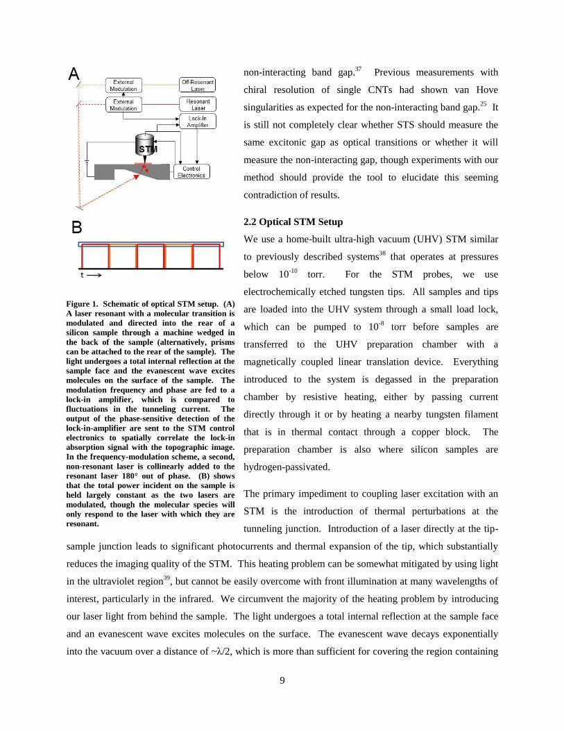
Chapter 8 : Deriving Thermodynamics from Kinetics ............................................................................ 60

: Laser Alignment ............................................................................................................... 69 Appendix A

: Experimental Procedures .................................................................................................. 71 Appendix B

: Matlab Code for STS Spectra Maps ................................................................................. 82 Appendix C

: Fitting Parameters for PTB1:4W ...................................................................................... 84 Appendix D

: Fortran Code for Singular Value Smoluchowski Dynamics ............................................. 87 Appendix E

: Fortran Code for Thermodynamics from Kinetics Fitting .............................................. 164 Appendix F

References ............................................................................................................................................. 181

1

Part I : Single molecule optical absorption by STM

Chapter 1: Introduction and Background

1.1 Methods for single-molecule optical detection

The vast majority of single-molecule experiments do not directly measure absorption, but rather infer

absorption from a secondary process such as fluorescence. This is because single absorbers usually have

an absorption cross-section which is very small relative to the experimental noise or the background

absorption. A large number of these types of studies have been performed on single carbon nanotubes

(CNTs) to gain information about their optical properties. With just a few exceptions, the vast majority of

these experiments has not directly measured optical absorption, but has instead relied on a secondary

process, namely fluorescence. While these experiments have provided much useful knowledge, they have

provided only indirect information about absorption. Moreover, while some molecules fluoresce

strongly, the techniques developed or used for these systems are not universally applicable since not all

molecules fluoresce.

Direct measurements of absorption of single CNTs have not been ignored because they are not

interesting, but because they have proved to be difficult experiments because the absorption cross-section

for a single-molecule is very small and because background absorption is relatively large, leading to a

major signal-to-noise problem. In 1989, the first single-molecule absorption experiment was done at

cryogenic temperatures with strong molecular absorbers1 and advances in the field have been relatively

slow. Room temperature single-molecule experiments have recently become plausible and there have

been a slowly growing number of techniques that examine systems on these scales.

Our lab reported the first example of room-temperature single-molecule optical absorption in 2006.2

Single-molecule absorption detected by scanning tunneling microscopy (SMA-STM) introduced a

technique that provided direct imaging of optical absorption of single molecules by monitoring laser-

induced changes in local electronic structure with a scanning tunneling microscope. This study employed

carbon nanotubes as the molecular absorbers and has served as the foundation for the work presented in

the following chapters. Shortly after this initial room-temperature demonstration, our lab presented a

frequency-modulation scheme that further cut-down on the background.3 In the few years since our lab

first demonstrated room-temperature single-molecule optical absorption, a handful of other single-

molecule techniques have emerged.

2

One method of room-temperature single-molecule absorption with low background relies on a

photothermal contrast mechanism.4 In this scheme, a modulated heating beam hits a sample causing local

thermal inhomogeneities where molecules are absorbing and leads to changes in the local refractive

index. A probe beam is then rastered over the surface and dips in transmission are monitored which result

from scattering at the locally heated regions. Another method has achieved single-molecule detection of

absorption using ground-state depletion microscopy.5 Here, two lasers at different wavelengths both

within a molecular absorption band are collinearly focused on a sample. One of the lasers is modulated

and if an absorption event occurs, the ground state of the molecule becomes depleted, which leads to a

modulation in transmission of the second laser. Finally, direct transmission measurements from a single

laser have also reached the single-molecule detection level. In this method, absorption images of single

molecules are taken by spatially dispersing the molecules in a sample and monitoring transmission losses

while rastering the sample through a tightly focused laser beam.6,7

Laser intensity fluctuations, which can

plague single molecule experiments, are accounted for by the use of a balanced photodetector with a

reference beam.

There have also been a few other studies in the past few years that have utilized carbon nanotubes as their

absorbers in single-molecule experiments. One technique required the growth of CNTs across a slit cut

into a silicon wafer. A laser was shined down the length of the slit and the sample was oscillated such

that the CNT translated into and out of the laser beam. The very small changes in transmission were

monitored by lock-in-detection at the oscillation frequency.8 In another technique, a photothermal

heterodyne imaging technique was used to excite CNTs with one laser and probe the induced local

heating field with another.9 Recently, this photothermal technique has been extended to single dye-

molecules as well, as discussed above.4

Despite having achieved room-temperature single-molecule detection, these methods still have some

limitations. All of these methods are still essentially diffraction-limited. As a consequence, they require

that molecules are still spatially distributed on their samples at a concentration low enough that

guarantees mono-dispersion. Even still, verification that an absorption measurement is a single-molecule

largely requires observation of phenomena such as blinking or one-step bleaching.

These articles which discuss single-molecule absorption point to each other, but not to our technique

described in the following chapters. Our technique, SMA-STM, offers several unique or complementary

advantages to other techniques. The primary advantage is the unparalleled spatial-resolution of optical

absorption, which can be directly imaged below the nanometer level. The method relies on measuring

absorption by monitoring changes in the local density of states and allows the simultaneous collection of

3

electronic and topographic information in addition to the optical signal. We can resolve optical

absorption well below the diffraction limit on a sub-nanometer scale. This, along with a demonstration of

our ability to differentiate absorption between two nanotubes that are directly adjacent to each other, are

detailed in Chapter 3.

1.2 Background on Optical STM Methods

The coupling of optical techniques with STM is not a new idea, though its evolution into mature

technologies has been more recent. Most of the research that couples STM with optical techniques have

utilized the introduction of laser excitation at the tunneling junction between the STM tip and sample in

order to examine a variety of phenomena. Much of the existing work is detailed at length in a review by

Grafström.10

Some of the highlights of that review as well as some additional more recent work is briefly

summarized here.

Under laser-illumination of the tunneling gap, a temperature difference can exist between the tip and the

sample, which leads to a thermovoltage across the gap.11

It is possible to leverage this to indirectly

examine differences in the local density of states on a sample due to differences in heating and therefore

the thermovoltage.12

Images can also be taken of difference mixing of multiple laser fields in a tunneling

junction.13

Surface states on semiconductors lead to a charge buildup. Optical excitation above the band gap of the

semiconductor creates carriers which disrupt the equilibrium, causing a potential referred to as the surface

photovoltage (SPV). The spatial variance of the SPV has been mapped in a number of studies on

different substrates, the first of which was on Si(111)-(7x7).14

The variation in local work function on a

surface can be monitored as well.15

Local photoelectron spectroscopy can be examined by collecting photoemitted electrons with an STM

tip.16

Recent work has shown that the light-induced tunneling current can be dissected into components

arising from excitation of carriers into the conduction band of materials as well as the SPV.17

Not only

can electrons excited by photons be monitored, but others have collected photons emitted by tunneling

electrons, which has recently been done on the submolecular level.18

Our technique, described in Chapter

2, is complementary to many of the techniques described above, but achieves optical absorption

measurements with superior spatial resolution.

1.3 The optical properties of carbon nanotubes

While carbon nanotubes (CNTs) were likely identified earlier,19

interest in them has grown substantially

over the past two decades since Iijima‘s well-recognized papers were published.20,21

Research on these

4

nano-materials has continued unabated because of their unique optical, electronic, mechanical, and

thermal properties. The work described in the following chapters examines some of the electrical and

optical properties, so they will be briefly reviewed here. There are a large number of different carbon

nanotubes, though the discussion here will be limited to the sub-class identified as single-walled carbon

nanotubes.

A CNT is an allotrope of carbon which is often described as a rolled up sheet of graphene, a monatomic

layer of graphite. Because of the hexagonal arrangement of atoms in graphene, there are a number of

geometric arrangements in which a seamless cylinder can be formed, each with varying diameters and

angles—known as the chiral angle—and of indefinite length. The electronic and optical properties are

directly related to the specific structure of the nanotube, specifically the diameter and the chiral angle.

The diameter and chiral angle for each possible CNT can be uniquely described by two indices n, and m,

where the vector around the circumference of the nanotube along the chiral vector is given by22

(1)

where a1 and a2 are the basis vectors in the real-space graphene lattice. From these two indices, simple

geometric relationships allow the diameter and chiral angle to be determined. Furthermore, the electronic

structure—and therefore the optical properties—of the CNTs are directly related to this information.

When the (n,m) indices satisfy the requirement that ‗(n-m) / 3 = integer‘ the CNTs behave as metals

whereas those that do not satisfy this requirement are semiconducting. The implication here is that in a

random distribution of CNTs, one third will be metallic while the remaining two thirds will be

semiconducting. This effect arises because the discrete linear wavevectors for CNTs allowed along the

axis of the nanotube on the first Brillouin zone overlap the K symmetry points of the 2D hexagonal

Brillouin zone of graphene. This model, which further allows for the prediction of electronic properties,

is known as the zone-folding method.22

In general, there is an inverse relationship between the diameter of CNTs and their bandgap and therefore

their optical transition energies. This has been shown both theoretically and experimentally.23,24

The

electronic structure that was predicted predominantly by tight-binding calculations indicated that all

CNTs had sharp spikes in their local density of states at particular energies related to their geometries.

These asymmetric areas of high state density, known as Van Hove singularities (VHS) were long

considered to be the source of electronic and optical transitions, an idea that was supported by some early

high-resolution STM electronic measurements.25

Semiconducting tubes were considered to have no state

density between the highest occupied VHS in the valence band and the lowest unoccupied VHS in the

5

conduction band. Until recently, it was thought that optical transitions in semiconducting carbon

nanotubes were band-to-band transitions between the VHSs, yet some convincing photoluminescence

experiments proved that there must be optically accessible states within the conventional band gap

predicted by these calculations.

The work that changed the interpretation of optical transitions were two-photon photoluminescence

experiments wherein CNTs were excited by a two-photon absorption process, after which photon

emission occurred at a substantially lower energy.26

The interpretation was that excitonic states existed

within the band gap of the CNTS. These excitons—Coulomb-bound electron-hole pairs—had binding

energies that made up a substantial fraction of the bandgap and were responsible for observed optical

resonances. 1-dimensional materials have excitons with even symmetry (s symmetry) with respect to

reflection along the nanotube axis, and odd symmetry (p symmetry). Owing to symmetry-based selection

rules, the s-states are one-photon allowed and the p-states are two-photon allowed. In a single-particle

model that does not account for excitons, both one and two-photon processes are allowed in the optical

transition to the continuum. In the picture presented by these experiments, two-photon absorption excited

electrons only to the higher-lying p-states or the band edge, after which the electrons relaxed to the

lowest-lying s-state where emission occurred.

While the realization that excitons, rather than band-to-band Van Hove transitions, were responsible for

optical processes in CNTs did not invalidate the body of work that led to the development of many trends

relevant to the photophysics of CNTs, it did open up new avenues for interpretation and exploration.

Subsequent calculations, utilizing the Bethe-Salpeter equation27

to account for the bound states, showed

that the exciton states had a finite confinement area and an expected symmetric absorption lineshape.28

The nature of optical transitions in CNTs arising from excitons had a number of implications guiding the

work presented here. Considering the difference in the predicted lineshape for exciton absorption and the

asymmetry present in VHS‘s, single-molecule absorption offers an opportunity to examine this

discrepancy. Because excitons have a confined local wave function, high-resolution experiments allow

for direct visualization of these states when pinned at defects. Because this work is all done under high-

electric fields, the presence of excitons introduces additional variables which must be considered

including field-induced binding-energy shifts and potential exciton dissociation. Not only would it be

difficult to ferret out some of this information from bulk experiments—particularly since the preparation

or purification of specific CNT chiralities has proved extremely difficult despite vast efforts—but much

of this requires experiments sensitive to a level below that of single structures.

6

The ability to resolve optical transitions on a scale smaller than a single CNT is also relevant because

carbon nanotubes are prone to structural defects. These defects can lead to the opening or closing of the

band gap locally, or result in a change in the density of states.29,30

7

Chapter 2: Optically-Assisted STM Instrumentation and Experimental Design

The combination of STM with optical excitation provides an opportunity to leverage both the high spatial

resolution inherent to STM with the spectral resolution of laser spectroscopy. Moreover, the STM

provides highly localized electronic measurements. This combination of tools yields a surface sensitive

technique that offers direct real-space imaging of absorption events with simultaneous temporal resolution

of correlated spatial, electronic, and optical properties on a sub-nanometer scale. Because of the high

resolution of this setup, we denote this optically-assisted STM technique Single-Molecule-Absorption

detected by Scanning Tunneling Microscopy (SMA-STM).

Optically-assisted STM experiments combine a conventional STM with laser sources. Only minor

physical modifications of an STM are required to allow the implementation of this technique. One or

more lasers are then coupled with the STM, which excite resonant features on the surface and the

resulting modification of the density of states is monitored via lock-in detection.

2.1 Basic STM Theory

In an STM, a sharp metallic tip is brought to within ~1 nm of a conductive or semiconducting substrate

and a bias is applied to the sample. Electrons tunnel quantum mechanically across the vacuum barrier at a

rate proportional to the local density of states and which depends exponentially on the size of the

tunneling gap. The tunneling current for a one-dimensional system at low voltage is given as

(2)

where It is the tunneling current, d is the distance between the tip and the sample, and κ is given by

√

(3)

where me is the electron mass and ϕ is the local effective work function, which is the average work

function for the tip and sample. This simple relationship was what allowed for the first experimental

STM imaging and was used in its interpretation.31

The practical application of Equation (2) for typical

values of ϕ is that a vertical change of tip position by 1 Å yields a change of an order of magnitude in the

tunneling current.32

Tersoff and Hamann established a theory based on the transfer Hamiltonian approach of Bardeen33

,

wherein they determined the tunneling conductance for an STM system in 3-dimensions. Considering

that real STM tips are not infinitely sharp, this formalism has important relevance to modern STM

applications. They showed that that the tunneling current is also linearly proportional to the local density

of states of the sample.34

This proportionality can be exploited to gather information about the local

8

electronic structure of surfaces and molecules, which will be described more in depth in the section on

Scanning Tunneling Spectroscopy.

We operate our STM at a constant tunneling current. The STM tip, rastered over the sample by four

quadrants of a piezoelectric cylinder, adjusts the tunneling distance when changes in the tunneling current

are induced by topographic or electronic variations in the sample. The sensitive z-adjustment from this

feedback loop is used to build the topographic image.

Scanning Tunneling Spectroscopy

Because the tunneling current in an STM is proportional to the local density of states, the STM can be

used to collect surface-sensitive local electronic information. The primary technique used for this is

known as Scanning Tunneling Spectroscopy (STS). In STS, the tip is positioned over a chosen spot on

the sample and the current feedback loop is then turned off. The voltage is then swept across a range

while the current is collected, which generates a current vs. voltage (I-V) curve.

The most fundamental piece of information that can be gained from the I-V curve is the band gap. For a

semiconductor at low sample bias, there may be no states from which or to which electrons can tunnel.

At these energies, the tunneling current will fall to zero and the width of that region in the I-V curve

corresponds to the band gap. Because this can be difficult to observe by eye, a plot of the logarithm of

the current makes the band edges readily identifiable and easy to measure.

Inaccuracies in the band gap measurement provided by STS can present themselves. The band gap can

often be overestimated by the procedure described above because at low bias the tunneling current will

drop off to a value below the sensitivity of the instrument despite the fact that states exist at that energy.

This can be corrected for by implementing a variable spacing method, wherein the tip steadily approaches

the surface as the bias approaches zero and retracts again as the bias increases with the opposite

magnitude. In this way, the tunneling current does not reach a negligible value until there are truly no

states into which to tunnel.

Less systematic, the band gap can often be inaccurate due to irregularities with the tip, most notably due

to an insulating oxide on the tip apex.35,36

When working on the Si(100) surface, we have a known band

gap of 1.1 eV, which acts as a standard to determine when the STS is producing accurate results for the

band gap. Moreover, we are often more interested in the relative difference in band gaps within a single

image, as we can compare this to the differential absorption that we observe.

STS has been used to probe the electronic properties of carbon nanotubes in a variety of studies. Of note,

recent STS measurements of CNT bundles were interpreted as showing the excitonic gap rather than the

9

non-interacting band gap.37

Previous measurements with

chiral resolution of single CNTs had shown van Hove

singularities as expected for the non-interacting band gap.25

It

is still not completely clear whether STS should measure the

same excitonic gap as optical transitions or whether it will

measure the non-interacting gap, though experiments with our

method should provide the tool to elucidate this seeming

contradiction of results.

2.2 Optical STM Setup

We use a home-built ultra-high vacuum (UHV) STM similar

to previously described systems38

that operates at pressures

below 10-10

torr. For the STM probes, we use

electrochemically etched tungsten tips. All samples and tips

are loaded into the UHV system through a small load lock,

which can be pumped to 10-8

torr before samples are

transferred to the UHV preparation chamber with a

magnetically coupled linear translation device. Everything

introduced to the system is degassed in the preparation

chamber by resistive heating, either by passing current

directly through it or by heating a nearby tungsten filament

that is in thermal contact through a copper block. The

preparation chamber is also where silicon samples are

hydrogen-passivated.

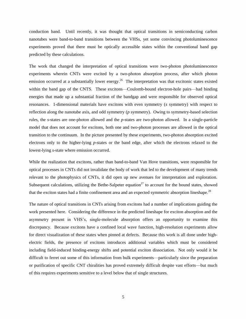
The primary impediment to coupling laser excitation with an

STM is the introduction of thermal perturbations at the

tunneling junction. Introduction of a laser directly at the tip-

sample junction leads to significant photocurrents and thermal expansion of the tip, which substantially

reduces the imaging quality of the STM. This heating problem can be somewhat mitigated by using light

in the ultraviolet region39

, but cannot be easily overcome with front illumination at many wavelengths of

interest, particularly in the infrared. We circumvent the majority of the heating problem by introducing

our laser light from behind the sample. The light undergoes a total internal reflection at the sample face

and an evanescent wave excites molecules on the surface. The evanescent wave decays exponentially

into the vacuum over a distance of ~λ/2, which is more than sufficient for covering the region containing

Figure 1. Schematic of optical STM setup. (A)

A laser resonant with a molecular transition is

modulated and directed into the rear of a

silicon sample through a machine wedged in

the back of the sample (alternatively, prisms

can be attached to the rear of the sample). The

light undergoes a total internal reflection at the

sample face and the evanescent wave excites

molecules on the surface of the sample. The

modulation frequency and phase are fed to a

lock-in amplifier, which is compared to

fluctuations in the tunneling current. The

output of the phase-sensitive detection of the

lock-in-amplifier are sent to the STM control

electronics to spatially correlate the lock-in

absorption signal with the topographic image.

In the frequency-modulation scheme, a second,

non-resonant laser is collinearly added to the

resonant laser 180° out of phase. (B) shows

that the total power incident on the sample is

held largely constant as the two lasers are

modulated, though the molecular species will

only respond to the laser with which they are

resonant.

10

molecules on the surface. One major disadvantage of this approach is that the substrate must be

transparent to the wavelength of illumination, though there are opportunities to expand this application to

a variety of wavelengths (see Chapter 4).

Silicon was the substrate used for the majority of the experiments shown here. We machined a 15° wedge

in the back of a boron-doped p-type Si(100) wafer by successive staircase cutting with a diamond dicing

saw. Subsequently, the wedge was polished with a Dremel and fine-grit alumina paste to create an optical

entryway for laser light that would then undergo total internal reflection at the front-face of the sample.

This wafer was then diced into appropriately sized-pieces for use in our sample holders. The clamps in

the sample holders have large slits cut in them to allow optical access to the wedge in the rear of the

sample. In the lab frame, the z (tip)-axis is horizontal, which allows the use of a normal optical table with

all laser beams operating at the same height. The angle at which the light strikes the silicon wedge is near

the Brewster angle, so p-polarized (parallel to the plane of incidence) light is preferentially transmitted.

The Fresnel equations written in terms of transmission for incident angles are

[ √

√

]

(4)

[ √

√

]

(5)

where Tp and Ts are the transmitted p and s light, n1 and n2 are the indices of refraction for the initial and

final media, and θi is the incident angle of the light40

. These relationships indicate that 91% of p-

polarized light and 44% of s-polarized light are transmitted into the silicon sample with our experimental

geometry. Figure 1 illustrates the geometry of the introduction of laser light through the rear of the

sample.

A tunable diode laser is used to excite molecules on the surface. It is overlapped with a helium neon

(HeNe) laser that provides visible guidance during the rough alignment process. Optionally, a second

diode laser of fixed wavelength can be used to further minimize differential heating (see 2.3 Signal

Detection).

11

Field Enhancement

A major advantage of the geometry of optically-assisted STM is that the tip acts to substantially enhance

the laser‘s electric field, allowing the use of modest laser powers.

Dr. Dong Xiao from the group of Professor Harley Johnson performed finite element calculations with the

COMSOL software package using parameters very similar to our experimental design. Infrared light

underwent total internal reflection in a medium with a dielectric constant of 12 to simulate a value close

to that of silicon41

both without and with a metal tip a few nm from the surface. Figure 2 illustrates the

results of the simulation. The leftmost panels show that the majority of the electric field and the energy

density do not penetrate beyond the surface. In the presence of a sharp metal tip, however, the evanescent

field is substantially enhanced within the tunneling region of the tip-sample gap. Other, more rigorous

calculations have shown that this field enhancement is on the order of 500-1000.42

The strength of the field enhancement depends strongly on the shape of the tip as well as the distance of

the tip from the surface. The distance-dependence of the field enhancement was directly visualized by a

group who used an STM in a front-illumination geometry to enhance the field of a UV laser to

depassivate hydrogen from a Si(100) surface.43

The size of their depassivated spot correlated with the

enhanced field and was strongly dependent on the tip-sample distance and also on the radius of curvature,

with sharper tips producing better results. Our electrochemical etching procedure produces a large variety

of tip shapes and sizes that may account in part for variations in the ability of the technique to detect

absorption.

Figure 2. Calculations of field enhancement for a silicon surface with infrared light undergoing total internal reflection.

The upper panels (A and C) show the field distribution and the lower panels show the energy density distribution (B and

D). The left side (A and B) is without the presence of a metal tip and the right side (C and D) is with a metal tip a few nm

from the surface. The local field enhancement in the tunneling junction is clearly visible.

12

2.3 Signal Detection

In conventional absorption spectroscopy, absorption is determined from a loss in transmission through a

sample. In SMA-STM, changes in the local electronic structure, and therefore the tunneling current, are

used to identify and spatially resolve absorption events. We modulate our lasers and monitor fluctuations

in the tunneling current at the modulation frequency with a lock-in amplifier while scanning to generate

an absorption image. We operate the lasers in either an amplitude modulation or frequency modulation

scheme. Full details of the laser alignment are given in Appendix A.

In the amplitude modulation scheme, the resonant laser is modulated between zero power and some

chosen power as a square wave. When using the tunable diode laser, we mechanically chop the laser

because the external cavity diode laser has a nonlinear response to an input signal, making the use of

electro-optic modulation cumbersome. In frequency-modulation, we introduce a second collinear laser

that is close in energy to the first, but non-resonant with the molecular transition. It is 180 ° out of phase

with the resonant laser and acts to keep the heating constant, but should play no role—or at least a lesser

role—in the modulation of the electronic density of states of the molecule on the surface. Figure 1B

shows how the total incident power is maintained at a constant level in this scheme.

The topographic image is given by the average tunneling current and the absorption image is given by the

lock-in detected modulation of the tunneling current that occurs faster than the STM feedback low-pass

cutoff. Regardless of whether an amplitude modulation or frequency modulation scheme is used, only the

laser resonant with the molecular transition should result in appreciable fluctuations in the tunneling

current at the modulation frequency. While some thermal fluctuations will result, the difference between

molecule and substrate in the lock-in image will be small. When the molecule is absorbing, however,

there will be relatively large current fluctuations when the tip is positioned over the molecule compared to

when the tip is over the substrate.

13

Chapter 3: Sub-nanometer Resolution of Optical Absorption in Individual CNTs

Portions of this chapter were previously published in:

Scott, G.; Ashtekar, S.; Lyding, J.; Gruebele, M. Direct Imaging of Room Temperature Optical

Absorption with Subnanometer Spatial Resolution. Nano Letters. 2010:10, 4897-4900.

http://dx.doi.org/10.1021/nl102854s

3.1 Introduction

We demonstrate here the ability to resolve optical absorption at the sub-nanometer level. To exploit the

high spatial resolution of the SMA-STM technique, we imaged two kinds of carbon nanotube (CNT)

systems. The first involves two CNTs in contact with one another, verifying that we can

spectroscopically distinguish adjacent nanotubes based on their electronic structure. To test the limits of

our ability to localize an optical signal, we then looked for carbon nanotubes containing a structural defect

clearly imaged by conventional STM. Defects in carbon nanotubes can significantly alter the local

electronic structure29

. We correlated the optical response with electrical (I-V) measurements, and showed

how direct visualization of excitonic absorption by the CNT can be used to measure penetration of the

exciton into the defect.

3.2 Results and Discussion

The experimental setup has been described in Chapter 2 and in refs 2,3

. The specifics for the sub-nm

resolution experiment are summarized here (additional details are given in 3.3 ). Experiments were

performed with a home-built ultrahigh-vacuum (UHV) STM similar to ones previously reported44

, using

electrochemically etched tungsten tips. P-type (boron-doped) Si(100) samples with a 15° polished wedge

in the back side were hydrogen-passivated in situ to produce a 2x1 reconstructed surface. HiPCO

produced carbon nanotubes were applied to the samples in situ using the dry contact transfer technique

with a fiberglass applicator.45

STM images were collected at a tunneling current of 50 pA and a sample

bias of -2 V.

To detect the λ11 absorption transition of a CNT, amplitude-modulated or frequency-modulated near-

infrared laser light was introduced through the wedge in the rear of the silicon wafer. Rear illumination

and wavelength modulation (by 50 nm) of the laser maximally suppressed thermal modulation of the

STM tip-sample junction.3 The light undergoes a total internal reflection (TIR) at the sample surface and

creates an evanescent wave that excites any resonant CNTs stamped onto the surface. A few mW of

laser power was sufficient to saturate the molecular transition because the sharp tip locally enhances the

electric field of the laser by a factor of 500-1000.42

The bulk of the tip is not illuminated by the TIR

geometry. The average tunneling current produces a conventional STM image. Simultaneously, a lock-in

14

amplifier (time constant 10 ms) demodulates the tunneling current

at the modulation frequency of the laser (1.2 kHz), thus detecting

changes in the local electronic structure due to resonant laser

excitation. STM and absorption images with sub-nm resolution are

thus obtained concurrently. The lateral resolution was measured to

be 0.40±0.05 nm (see Figure 7).

Figure 3 illustrates differentiation of two directly adjacent

nanotubes by room temperature optical absorption. The laser

energy (1.03 eV) is in the range of the λ11 lowest energy absorption

band of 1 nm diameter carbon nanotubes. The entire image shown

is approximately 500 times smaller than the focused size of the

diffraction-limited near-IR spot. Figure 3a shows a derivative of the

conventional STM topographic image of two semiconducting

carbon nanotubes nearly in contact on a hydrogen-passivated

Si(100)-2x1 reconstructed surface. Figure 3b shows the SMA-STM

absorption image, collected at the same time. Only the carbon

nanotube on the left absorbs at 1200 nm. The horizontal streaks in

the middle of the topographic image are a result of the CNT on the

right moving ~ 1 nm towards the left CNT in the middle of the scan.

Thus the right nanotube is strongly interacting with the tip, but not

with the laser. Figure 3c shows the two CNTs after the right tube

has moved.

Based on its chirality, its diameter, and the absorption wavelength

of 1200 nm, the carbon nanotube on the left can be identified as one

of two types. The spatial derivative of the STM topography image

in the inset of panel 1a reveals a chiral angle of 13±1°. The

measured topographic height was 0.9±0.1 nm. Based on data from

an empirical Kataura plot,24

we can assign the absorbing CNT to

either a (10,3) tube (12.73° chiral angle, 0.936 nm, λ11=1249 nm) or

less likely a (11,3) tube (11.74° chiral angle, 1.01 nm, 1197 nm).

All other identities can be confidently excluded.

Although optical discrimination without photoswitching between

Figure 3. Differentiation of molecules

separated by a few nm by optical

absorption. (a) Topographic derivative

image of two carbon nanotubes in close

proximity. Inset: enhanced image

showing the carbon lattice of the

nanotube on the left. The red vectors

show the chiral angle of 13°. Scale bar is

5 nm. (b) Simultaneously collected lock-

in absorption image under 1200 nm

laser excitation showing absorption by

the left nanotube and no absorption by

the right nanotube. (c) Subsequent

topographic image showing the two

carbon nanotubes in contact after the

right tube was lifted by the tip.

15

similar molecules separated by a few nm is a novel capability,

Figure 4 illustrates that we can identify variations in absorption

even within a single nanotube, and correlate these variations with

electrical and excitonic properties. The topograph in Figure 4a and

the lock-in absorption image excited at 1200 nm in Figure 4b were

collected simultaneously. The topograph shows individual dimers

on the Si(100)-2x1 hydrogen passivated surface, as well as some

dangling bonds near the CNT. Near the central part of the CNT, a

structural defect causes the apparent height of the nanotube to

increase. The absorption image shows no differential absorption

signal relative to the substrate at the defect location, while the rest

of the CNT strongly absorbs at 1200 nm. Thus the local bandgap

of the CNT has shifted below the 1.03 eV laser energy at the defect

site. Figure 4c shows the lock-in amplifier signal 90° out of phase

with the laser modulation. Aside from a small amount of noise

induced as the tip undergoes feedback to move over the edge of the

CNT46

, there is no net signal observed relative to the substrate.

This observation verifies that the detected absorption image is

phase-sensitive relative to the laser modulation, and that thermal

effects are minimal: thermal modulation would show up with a

phase lag (residual signal at 90°), while the absorption signal is

modulated essentially instantaneously on the ms time scale of the

modulation (τrelax <<1 ms for CNTs47

).

We can directly compare the optical absorption with the

electrically measured bandgap. Scanning tunneling spectroscopy

(STS) was used to measure I-V curves from -2 to +2 V at each red

and blue point in Figure 4a between two of the laser absorption

scans. Figure 5 shows the resulting bandgaps as a function of

distance along the trace. Moving from substrate to CNT along the

blue trace, the bandgap narrows suddenly, defining our lateral

resolution of ±0.1 nm. The red trace shows the bandgap narrowing

more gradually along the tube. The defect bandgap shrinks by

about 40% compared to rest of the molecule, pushing the optical

Figure 4. Sub-nm absorption image of a

defected single-walled carbon nanotube.

(a) Topographic image of a carbon

nanotube showing a defect along its axis.

The blue and red circles correspond to

points at which scanning tunneling

spectroscopy was performed (see Figure

5). Scale bar is 2 nm. (b) Absorption

image taken under 1200/1300 nm

excitation by frequency-modulated laser

excitation. The defect from (a) shows up

as a decrease of the absorption signal over

a 2 nm length of the CNT. In (c), the

lock-in amplifier phase was rotated 90

degrees from that in (b). No significant

absorption relative to the silicon

background is observed even though the

vertical scale of the image is expanded to

highlight the noise floor. The phase of (b)

and (c) was adjusted by 180° to yield a

similar gray-scale as in Figure 3b for

comparison.

16

transition out of resonance with the 1200 nm excitation laser. The bandgaps measured by STS are

overestimated here, likely due to an insulating oxide on the apex of the STM tip. Using the silicon

bandgap as a reference and rescaling it to 1.1 eV, the CNT bandgap away from the defect scales to ~1.0

eV, commensurate with the excitation laser energy. Unlike an I-V curve, the optical absorption signal can

be collected simultaneously with a conventional STM scan to spatially resolve such defects and

characterize their bandgap in high throughput.

We used the result in Figure 4 to visualize directly exciton penetration into the defect. Optical absorption

in the λ11 band yields a bright excitonic state with a probability envelope exp[-x2/σ

2],

26,48,49 with σ

proportional to the diameter of the CNT. The 1200 nm laser generates excitons at all points along the

CNT except in the non-resonant defect. Excitons generated adjacent to the defect delocalize into the

smaller bandgap region. Figure 6 shows a fit of the normalized absorption signal along the tube axis to

(6)

where x is the distance along the carbon nanotube axis illustrated by the red line in the inset of Figure 6.

We measure σ' = 0.9±0.3 nm (accounting for the lateral resolution), which defines the penetration depth

of the exciton into the defect region. The off-resonant bandgap in the defect reduces the penetration depth

of the edge exciton compared to the width of a free exciton (assuming the defect does not substantially

alter the dielectric constant). By solving the non-linear Schrödinger equation for a room temperature

exciton propagating into the low-bandgap region of the defect, we find σ /σ‘= 2.0 for the exciton size-to-

Figure 5. Scanning tunneling spectroscopy traces. Spatially-resolved maps of current-voltage scans that correspond to

the blue (a) and red (b) dots in Figure 4. The band gap (dark blue) narrows from silicon substrate to nanotube (a), and at

the defect site on the nanotube (b).

17

penetration ratio and therefore σ = 1.8±0.6

nm for the exciton size. For a 1 nm diameter

CNT, theoretical predictions put the size of

an exciton close to σ = 1.5 nm49-51

. Our

result agrees within uncertainty with this

prediction. Previous experimental work,

which extracted the exciton size from a

reduction in oscillator strength using pump-

probe spectroscopy, found a value of 2 nm

for the size of excitons in a (6,5) nanotube,

considerably larger than the theoretical

prediction of 1.1 nm52

.

In summary, optical absorption can now be

imaged at room temperature with sub-nm

resolution. It can distinguish similar

molecules in direct contact. The signal

depends on laser excitation, not on which

molecule more strongly couples with the tip.

The onset of absorption can be imaged within a single nanotube, quantifying exciton spatial penetration

into a CNT defect and allowing exciton size to be evaluated.

3.3 Experimental Conditions

For the data presented in Figure 3, one laser was used and amplitude-modulated at a laser power between

0 and 3.9 W/cm2. The modulation and lock-in frequency was set to 1.2 kHz with the laser operating at

1200 nm. The lock-in amplifier time constant was 10 ms and the STM tip velocity was 20.1 nm/s. This

time constant/scan rate combination minimized any ‗smear‘ of the absorption image. Our resolution

analysis (see Figure 7) shows that the optical resolution is similar to the current image resolution, limited

by the tip.

For the data presented in Figure 4 and Figure 5, two lasers were used to allow frequency-modulation of

the incident laser light over a wide frequency range. The resonant laser was operated at 1200-1240 nm

and modulated from 0 to 1.5 W/cm2 at 1.9 kHz. The off-resonant laser was operated at 1300 nm and

modulated exactly 180° out of phase from 0 to 10.7 W/cm2. The lock-in amplifier time constant was 3 ms

and the tip velocity was 14.8 nm/s. The resonant laser was unpolarized, with residual polarization at the

Figure 6. Exciton penetration into the defect. The normalized (0 to

1) lock-in absorption signal is shown in black, progressing from the

defect region on the left to the absorbing region on the right. The

Gaussian decay fit of the exciton penetration is shown as a red solid

line, yielding ‟=1.0±0.3 nm in eq. (1). The range of the x-axis is

illustrated as a red 4.5 nm scale bar in the inset, which reproduces

a detail from Figure 4b.

18

sample due to the internal reflection process. The off-resonant laser was polarized in the s-plane with

respect to the wedge. The maximum powers of 1.5 and 10.7 W/cm2 (different to account for polarization-

dependent reflection of both lasers) were chosen to eliminate modulated substrate or tip heating by the

two lasers.

The band gap trace was generated by measuring log(abs(I)) versus V traces obtained at each position (red

or blue points in Figure 4a). At each of these positions, 50 I-V traces were averaged with an initial

current of 0.3 nA and a variable spacing with the tip approaching the surface by 2 Å as V0 with the

STM feedback disabled. When the current flow becomes negligible (below ~10-14

A), the voltage lies

within the band gap and is shown in Figure 5 as dark blue. Relative band gaps were measured at initial

set-point currents of 0.3 nA, but absolute gaps in the I0 limit may be slightly lower.

3.4 Exciton Analysis

To measure exciton penetration, six cross-sections averaging 5 pixels wide were taken along the axis of

the nanotube for both the forward and reverse scan directions on both sides of the defect, resulting in 24

traces showing signal decays into the defect region. A Gaussian decay (6) was fitted to each of the 24

traces and we discarded 7 low-signal traces whose noise caused the standard deviation of the fit to

increase. The trace shown in Figure 6 is an average of the remaining 17 traces weighted by their fitting

error and offset horizontally to center the Gaussian peak at zero. The reported uncertainty is one standard

deviation of the mean of the 17 fitted values of σ. A Gaussian envelope is strictly only valid for a free

Figure 7. Minimum resolution was estimated by measuring profiles of the topographic and absorption image

perpendicular to the carbon nanotube axis away from the defect. The estimated σ value (using the same units as for

exciton width) is 0.40±0.05 nm, less than 1 nm. This broadens a 1 nm measured width by < 10%.

19

exciton with a quadratic energy-momentum dependence, but a sigmoidal (exponential penetration) fit

gave a very similar length scale.

The reduced band gap of the defect provides an effective barrier into which the exciton tunnels, reducing

its size and distorting the shape from a Gaussian. To model the exciton, we solved the nonlinear

Schrödinger equation describing the propagation of a soliton wave with σ≈1.7 nm into the effective

barrier. Propagation along the CNT axis was modeled in one dimension, and the kinetic energy of the

soliton was set to the thermal energy (kBT at 298 K). Figure 8 shows the solution for the free soliton, and

the narrowing of the soliton as it penetrates into the band gap. In accordance with Figure 5, the band gap

energy along the tube was modeled as a function of position as a 2 nm wide Gaussian dropping by 40%

from the value outside the defect. The maximum tunneling depth calculated for the soliton was σ' = 0.85

nm, yielding the σ/σ‘ = 2 ratio. Deconvolution of the tip response yields σ' = 0.9 nm for a measured width

of 1 nm (Figure 7), and applying the computed 2:1 ratio, we obtain σ =1.8 nm for the width of the

unperturbed exciton.

Figure 8. Model exciton propagation with the nonlinear Schrödinger equation. Top: freely propagating exciton at energy

kBT (T=298 K) retains constant width (center of wavepacket probability shifted for comparison). Bottom: exciton

propagating into a bandgap reduced by 60% has a width reduced by one half (0.85 nm) compared to unperturbed exciton

(1.7 nm).

20

Chapter 4: Broadband Substrates for SMA-STM

The use of silicon as a substrate for SMA-STM is ideal for many cases. Pristine surfaces can be prepared

in situ, the substrate provides a reliable reference for STS measurements, it is a well-studied system with

CNTs, and it is easy to machine a wedge for our rear-illumination scheme. The primary problem with

silicon is that its 1.1 eV band gap prevent us from using our rear-illumination geometry with light above

that energy. Our experiments are restricted to the infrared, which leaves out the important and interesting

spectroscopic regions of the ultraviolet, visible, and very near infrared.

Alternative substrates that provide a broadband platform for SMA-STM must meet several requirements.

They must offer optical transparency across a broad wavelength range, be conductive for use in an STM,

and must have excellent flatness so that molecules can be readily resolved. We have pursued two primary

classes of potential substrates that meet these requirements: ultrathin metal films and graphene on

transparent substrates.

4.1 Metals Films on Sapphire

Metal films have long been used as STM substrates because they can be prepared atomically flat and are

highly conductive. These single-crystal films that have superior smoothness are typically at least

hundreds of nanometers thick,53,54

rendering them opaque and therefore useless for rear-illumination

optical STM. At thicknesses under ~20 nm, ultrathin metal films still allow substantial light transmission

across a broad wavelength range. The difficulty in preparing ultrathin films is in acquiring optimal

flatness.

Prior work in our lab established the best parameters for room-temperature growth of ultrathin metal films

on sapphire.53

While these films met requirements of flatness, conductivity, and optical transparency for

SMA-STM, their flatness was not ideal for most experiments. Our previous work had indicated that the

induced temperature profile during deposition was a controlling variable in the film flatness, yet active

control of the substrate temperature had not been undertaken. Björn Braunschweig suggested that for

ultrathin platinum films, active heating of the substrate could substantially improve the flatness. As a

result, we pursued elevated temperature growth of ultrathin platinum and gold films to achieve the

optimal balance of flatness, transparency, and conductivity. This work required customizing a UHV

heater for installation in an electron-beam evaporator.

Heater Design

The electron-beam evaporation (e-beam) system that we used for thin-film growth was not equipped for

thermal control of substrates. It did, however, have a set of electrical feedthroughs that allowed for the

easy introduction of a substrate heater. The e-beam was a CHA-SEC 600 in the clean room at the Micro

21

and Nanotechnology Laboratory at the University of Illinois. We combined a commercial substrate

heater with a custom mounting and electrical connection apparatus to provide variable temperature

heating of substrates during metal film deposition within the e-beam.

We purchased a ½‖ 1200 °C molybdenum heater from Heatwave Labs with a heat shield assembly and

sample clips (part no. 101491-04). We mounted the backside of the heater to a cylindrical copper block,

which acted as an additional heat sink to prevent overheating locally within the e-beam instrument. The

copper block was then mounted to a 6‖ long stainless steel plate through a set of MACOR washers and

screw insulators. The electrical insulation was required because the body of the heater is one of the heater

leads and could not be allowed to short to the body of the e-beam instrument. The steel plate was allowed

to rest on top of the 4‖ hole in the e-beam that is designed for mounting 4‖ wafers. Figure 9 shows a

schematic of the heater apparatus that can be mounted in the e-beam instrument.

The steel plate and the copper plate were machined with holes that allowed the passage of wires for the

bias of the heater as well as the application of a thermocouple behind the sample face. The heater wires

and thermocouple wires were connected to larger gauge wires for connection to the feedthrough. These

larger bare wires were insulated with 1‖-long double-bore ceramic tubes. Each set of these was mounted

Figure 9. Schematic of the heater apparatus used to control the substrate temperature during e-beam metal film

deposition. The heater assembly steel plate rests on the lip of a 4-inch diameter hole in the e-beam chassis which would

normally be used to mount substrates on 4-inch wafer plates.

22

with a bracket to the steel plate to minimize strain on the smaller, more fragile wires that connected to the

body of the heater. The connection wires were each fitted with alligator clips for easy installation and

removal of the heater apparatus to the feedthrough leads.

We originally purchased type-K thermocouples from Heatwave Labs, but they were very fragile and

broke easily if they had to be removed from the assembly. For a fraction of the cost, we were able to

make our own thermocouples by feeding 0.003‖ alumel and chromel wires through a double-bore ceramic

tube with 0.005‖ inner-diameter bores. After making the thermocouple junction, we coated the junction

with Ceramabond 571 to provide electrical insulation, but thermal conductivity, so that the thermocouple

could be inserted directly behind the heater face.

Elevated Temperature Growth of Platinum Films

When the sapphire substrate is actively heated during deposition, atomically smooth islands begin to

form. The size of the islands as well as their heights increases with increasing temperature. At the same

time that the islands grow larger, the resistances of the films increases until the films become

Figure 10. Comparison of platinum films grown at various substrate temperatures. (A) is 10 nm and (B) and (C) are 15

nm, but room temperature films at 15 nm have the same morphology. As the temperature increases, the islands grow

larger, but the film resistance increases. “Moderate” temperature here is ~ 700 °C. The thermocouple measurement for

the “high” temperature film was inaccurate, but it was grown at a higher heater power dissipation than the film in (B).

The film in (C) was non-conductive.

23

discontinuous and non-conductive. Figure 10 clearly demonstrates this trend of increasing island surface

area and increasing film resistance. The growth mode for these films is a Volmer-Weber growth, as the

metal atoms are more attracted to each other than to the substrate.55

At room temperature, when the metal

atoms lacked sufficient energy to nucleate and aggregate, the growth-mode had appeared to be more

layer-by-layer.

This temperature trend can be reproduced to some degree by heating films after deposition. Room

temperature films which are flame-annealed do not tend to produce atomically smooth islands, though

they do show aggregation. Starting with flat islands, however, and annealing with a hydrogen-oxygen

flame produces results like those shown in Figure 11. With additional heating, the islands grow taller and

larger, but the areas without metal between the islands also grow larger, leading to disruptions in

conductivity.

Figure 12 shows a 15 nm platinum film grown at ~700 ° C. This temperature falls into the range of

―intermediate‖ temperatures for platinum where the size of the flat islands is reasonably large, but for

which the film still maintains conductivity. Figure 12A shows an AFM image of the as-grown film. B

shows an STM image on which smaller, atomic steps of Pt are visible. C shows how clearly resolved a

Figure 11. Effects of flame-annealing on ultrathin Pt films. The as-grown film in (A), which corresponds to Figure 10C,

was annealed with a hydrogen-oxygen flame. In the “gentle” anneal, the flame was gently brushed over the surface and in

the “aggressive” anneal it was more closely swept over the film where a color change was visible to the eye. With the

added heat, the islands grew larger and taller.

24

CNT is on the flat surface. D shows a normalized histogram of the pixels in the boxes overlaid on panel

B. Fitting a Gaussian to each peak in the histogram gives a step height of 2.37 Å. For Pt(111), the step

height is 2.3 Å and others have measured an electronic step height of 2.36 Å on a single-crystal Pt

substrate.56

This is a good indicator that our ultrathin Pt films on sapphire are growing in a (111)

orientation.

The STM image shown in Figure 12B was taken within a few days of the film being grown and was

degassed in the UHV prep chamber by bringing the sample holder into thermal contact with a copper

block at ~100 °C. The image in panel C was taken several months after that in panel B and the sample

was hard to scan and appeared dirty after reintroducing it to the UHV-STM after it had been allowed to sit

in ambient conditions. The scanning conditions improved drastically by direct resistive heating, passing

current through the platinum film itself. AFM performed after removing the sample from the STM

showed no noticeable changes to the film morphology due to the resistive degas.

Figure 12. Scanning probe microscopy of flat, conductive Pt film. (A) shows an AFM image of a 15 nm deposition of Pt

that corresponds to the film in Figure 10B. (B) shows an STM image of the same film where multiple atomic steps are

visible on top of the larger terraces. (C) illustrates a CNT (most likely with a second CNT bound to it at the lower half) on

the substrate. (D) shows a normalized histogram of the height values for each pixel in the red and black boxes in (B). The

blue and magenta curves are Gaussian fits to the histogram and their peaks are 2.37 Å apart, indicating that the steps are

monatomic in height and match the expected step-height for a Pt(111) surface.

25

We were able to make very thin, conductive platinum

films by depositing 5 nm of Pt at room temperature, then

immediately heating the sample to over 300 °C. Figure

13A shows an STM topography of such a film with a

CNT that was deposited via dry contact transfer. It

should be noted that while CNTs can be resolved on this

surface, films like those shown in Figure 12 have

superior flatness that will be more suitable for smaller

molecules. While not universally true, many of the

CNTs we have examined on ultrathin metal surfaces

tend to have narrower band gaps and a taller apparent

height in the STM than we observe on silicon. Figure

13B and C show some representative spectra and height

profiles that illustrate this effect. While the data shown

in these figures is not extremely far from expected

values, we see this trend with large consistency,

indicating that the metal surface may be doping the

CNTs with additional state density.

Elevated Temperature Growth of Gold Films

Both platinum and gold make an excellent choice for

thin films for SMA-STM substrates because they are

noble metals and do not oxidize. Gold has a few

characteristics which make it more desirable than

platinum if it is possible to develop thin films with the

same flatness. For comparable thicknesses, gold has

slightly better optical transmission than platinum.57

Furthermore, gold can act as a support for self-

assembled monolayers of alkanethiols or other thiol

derivaties which could be functionalized as anchors for

molecules that do not physisorb well to the metal surface.58

The previous room-temperature work from our lab all revolved around gold,53

so we set out to develop

gold films at elevated temperature in order to create flatter films in the same way that we did with the

platinum. The same general trends that we established for elevated temperature deposition of platinum

Figure 13. Characteristics of CNT on ultrathin

platinum. (A) shows an STM topography of a CNT

on a 5 nm Pt film grown at room temperature, then

elevated to over 300 °C. The spectra map in (B)

corresponds to the blue points in (A) and the height

profile in (C) is an average cross section depicted by

the line labeled „1‟ in (A).

26

held true for gold as well. At higher temperatures, the islands grew larger, but the conductivity of the

films grew smaller. There were some substantial qualitative and quantitative differences between the

platinum and gold films, however.

For comparable film thicknesses and deposition temperatures, the gold films produce smaller islands than

the platinum films. Morphologically, the gold films tend to aggregate into isolated polygonal structures

with straight edges. The platinum films, in contrast, have more rounded edges and the isolated structures

merge into extended structures that wrap around each other. Additionally, the gold films become non-

conductive at lower temperatures and with smaller islands than the platinum films.

For many of the gold films studied here, their semi-transparent appearance takes on a color other than

gold. Our elevated temperature films most often take on a blue hue, though some regions of pink have

also appeared. This can be seen in the photograph in Figure 14D. Thin gold films can take on a variety

Figure 14. Comparison of gold grain sizes as a function of temperature. (A) and (B) are AFM topographs from the same

sample that had variations in the color, likely due to local temperature inhomogeneities across the sample during

deposition. (A) shows a region that appeared gold in color to the eye and (B) shows a region that had a bluish tint to it.

(C) is a histogram showing the size of the islands in each region. The bars are offset for clarity, but the binning was

identical for each data set. (D) is a photograph of two gold samples of the same thickness deposited at different

temperatures. The sample on the left demonstrates the blue color that arises from the island formation of the elevated

temperature films.

27

of colors depending on their morphological structure, a result that arises from the excitation of a plasmon

resonance.57,59

This aspect of the gold films is undesirable for broadband SMA-STM substrates because

the plasmon excitation arises from absorption. For films of a blue color, the plasmon absorption peak is

in the red.

Not only can the film colors and morphologies vary from film to film, but in some cases, it will vary

within a single film. In one sample, shown in Figure 14A and B, the film appeared gold in some regions

and blue in others. As expected, the islands were larger in the region that appeared blue than in the region

that appeared gold. Figure 14C shows a histogram comparing the sizes of the islands in the AFM images

in panels A and B. The blue area had more larger islands and fewer smaller islands than the region that

appeared gold to the eye.

In order to find a compromise between flatness and conductivity, we grew variable temperature gold

films. We first deposited a conductive layer of gold at room temperature, then applied a second layer at

elevated temperature to provide flat islands for SMA-STM. These films too became discontinuous and

control experiments proved that heating a room temperature gold film caused aggregation and island

formation—though more rounded than flat on top—that led to a lack of electrical conductivity.

To overcome the problem with the underlayer of metal coalescing, we grew films that were gold on

niobium instead of gold on gold. Niobium has a substantially higher melting temperature than gold—

2477 °C vs 1064 °C60—which should prevent the elevated temperature from leading to substantial

diffusion. Additionally, a seed layer of Nb can be used to reduce lattice strain and has been used to make

ultrathin gold films before.61

To date, we have been unable to reproduce the results of ref. 61

. Others have

argued that the seed layer does not aid in the production of the films through a decrease in the lattice

mismatch, but rather by changing the interaction energy with the substrate.62

Interestingly, for the films that we have grown to date, we have had difficulty producing islands of gold

with the flatness we achieved with gold directly on sapphire. These films are, however, more conductive

at comparable thickness than the gold on sapphire without the seed layer.

4.2 Graphene on Transparent Substrates

Ultrathin metal films are not the only theoretically feasible avenue for satisfying the criteria of substrates

for SMA-STM. Graphene, a single monatomic layer of graphite, has the potential to offer a platform with

excellent flatness, high electrical conductivity, and broadband optical transparency. Even with just a

monolayer of graphene supported on a transparent substrate, it should be possible to perform optical STM

28

experiments. There are a number of ways that such a substrate

could be produced and we have explored some of those

possibilities.

Since its first isolation63

, graphene has garnered substantial

research interest due to its unique electrical properties as a 2-

dimensional system. Graphene is described as a semi-metal

because its valence and conduction bands just touch at the K

points in reciprocal space, offering a direct conduction pathway.64

The practical result of this electronic structure is that graphene has

very high carrier mobilities and a single sheet can have very low

resistance.65

Moreover, graphene only absorbs 2.3% of light per

monolayer66

, which makes it an ideal candidate for SMA-STM at

a variety of wavelengths since single or few layer films are readily

possible.

There are many methods for the production of graphene, an area

of research which is continuing to grow rapidly. Chandra

Mohapatra from the group of Jim Eckstein produced graphene on

sapphire and graphene on silicon carbide substrates using

molecular beam epitaxy (MBE). In their method, an electron gun

vaporizes a solid carbon source in a UHV chamber to produce a

molecular beam of carbon, which deposits onto a substrate.

During the deposition, the epitaxial growth of the graphene is

monitored by reflection high energy electron diffraction

(RHEED). The film quality and thickness are later examined

using Raman spectroscopy, x-ray photoelectron spectroscopy

(XPS), and AFM.

We performed STM on several of these samples, searching for the

flatness that would provide an excellent platform for SMA-STM. We were unable to perform STM on

the graphene grown on sapphire despite the fact that the samples had resistances on the order of MΩ after

growing Ti/Au contacts at the edges. We believe that while there was a percolative pathway for carriers

to travel across the sample, the probability of bringing the STM tip onto this pathway rather than an

isolated region of graphene islands was small.

Figure 15. STM images of graphene

grown on silicon carbide by molecular

beam epitaxy. This sample lost epitaxy

during growth. The scale bars are 50 nm

in (A), 5 nm in (B), and 2 nm in (C).

29

We were, however, able to perform STM on several samples of graphene grown on silicon carbide. We

were able to degas the samples through the silicon carbide to achieve high temperatures and achieved

near-atomic level resolution. Figure 15 shows STM images of an ~7 monolayer growth of graphene on

silicon carbide. According to RHEED measurements, the sample lost epitaxy during the MBE growth. In

Figure 15B and C, a mixture of graphene lattice and Moiré patterns can be seen and sheets of graphene

appear to curve over the surface which appears to undulate under it.

Figure 16A and B compares the sample from Figure 15 to another sample which was only a few

monolayers and maintained epitaxy according to RHEED measurements during the MBE growth. The

overall roughness of the sample in B is lower, but it still shows many discreet regions indicating that the

growth mode was not layer-by-layer (Frank van de Merve), but was instead more island-like (Volmer-

Weber).55

There is a promising alternative to producing graphene on transparent substrates that will be monatomic

and more largely continuous that we are pursuing in collaboration with Josh Wood from the groups of Joe

Lyding and Eric Pop. This involves growing large sheets of graphene on copper and transferring them via

a polymer transfer method onto a transparent substrate such as sapphire. The growth of graphene on

copper restricts the formation to almost exclusively monolayer graphene because the chemical vapor

deposition (CVD) growth can only catalyze on the copper surface.67

Once the surface is saturated, no

additional growth can take place. The monolayer graphene can then be transferred to arbitrary

substrates.68

Figure 16. Comparison of two graphene on SiC surfaces by STM. The graphene surface in (A) corresponds to Figure 15

and lost epitaxy during growth. The surface in (B) maintained epitaxy according to RHEED measurements, but

maintained an island-like structure.

30

Chapter 5: Spectral Resolution (Factors affecting absorption)

Single-molecule spectroscopy faces inherent challenges related to signal to noise. Each choice of

detection method brings its own complications that must be understood in order to interpret meaningful

results from experiments. While SMA-STM is largely straightforward in its implementation, the use of

an STM as a detector of optical absorption does introduce its own complexity. This chapter will discuss

the collection of single-molecule spectra as well as the factors that may influence the results.

5.1 Collecting Optical Spectra

For single molecules, the observation of optical absorption with high spatial resolution as demonstrated in

Chapter 3 becomes much more interesting when we can compare the intensity of absorption across a

range of wavelengths. This is the traditional methodology of absorption spectroscopy and its use in

single-molecule spectroscopy serves many purposes. Measuring a lineshape for an absorption peak for a

single molecule provides a wealth of information. In comparison to bulk experiments, a single-molecule

spectrum can elucidate the contributions of homogenous and heterogeneous broadening. It can resolve

differences between individual molecules, which is particularly relevant for structures without finite size

such as carbon nanotubes. Moreover, it can give information about the influence of the local environment

on the optical properties.

For CNTs in specific, there have been many different lineshapes measured or predicted. Van Hove

singularities have a very specific asymmetric lineshape,69

while Rayleigh scattering experiments have

provided a different asymmetric lineshape.70

Excitons, however, should have a Gaussian envelope.28

Our

method provides a tool that should be able to determine the absorption lineshape for single molecules

with high resolution.

Automated spectra collection

The major difficulty in SMA-STM experiments that provide a spectrum arises from the need to have

multiple variables functioning together for a long enough period of time to collect an entire spectrum.

The lasers must be properly aligned, the CNTs must be absorbing in the laser wavelength range, and the

STM tip must maintain high imaging fidelity throughout the collection. For this last reason, it is

important to be able to collect spectra quickly to minimize the probability of changes to the tip.

We have set up an automated method for tuning the resonant laser. Our tunable laser from Sacher

Lasertechnik can be tuned across a range of 1156-1265 nm. The outputted wavelength is adjusted by a

grating which is rotated by an inchworm motor. This motor is controlled via a serial interface through a

piece of software written in Labview and provided by the manufacturer. The laser diode current, and thus

the laser power, is controlled by the laser power supply, which interfaces with a computer via GPIB.

31

The software provided by Sacher Lasertechnik does provide a primitive automated tuning capability,

which allows the user to tune the wavelength to a list of values either on a regular time schedule or by

interacting with the program. This was not sufficient for our needs because we needed to correlate our

wavelength changes with the end of an STM scan, which would not always be on regular time intervals

and we wanted the data collection to be automated. More importantly, maintaining a constant laser power

as the wavelength is changed requires adjusting the laser diode current because the diode output power is

not uniform across the tuning range. We modified the program to overcome these shortcomings in the

provided design.

Professor Joe Lyding modified the STM software to output a voltage pulse at the end of each scan in a

batch mode, which is the mode on our STM which allows the auotmated collection of images. We

modified the Labview program from Sacher to monitor for these voltage pulses through an oscilloscope

that communicates via GPIB. When a voltage pulse is detected, a serial command is sent to the laser to

tune the wavelength and a GPIB command is sent to adjust the laser diode current. The laser diode

current adjustment is determined from a calibration curve of laser powers as a function of current at each

of the used wavelengths. We also modified the software to record all of the data and the actual laser

Figure 17. Mechanism of automated spectrum collection in SMA-STM. (A) shows the interface for the laser tuning based

on voltage pulses. (B) shows sample laser diode calibration curves for the selection of uniform laser powers at different

wavelengths. (C) is a schematic of how the instruments and software communicate with each other for automation.

32

power of a dumped beam from the beam splitter, so that it can be compared to the STM files saved in the

batch mode.

Figure 17 shows how this automation takes place. Panel A shows a screenshot of the software interface

and B shows an example of the power vs diode current tuning curves. C shows a schematic of how all of

the pieces of equipment and software interact with each other during automated spectra collection. The

implementation of this in the Labview code was straightforward, though the details of the code are

covered under a non-disclosure agreement with Sacher Lasertechnik.

In many cases, it is not important to collect large square images to get spectral information. In these

cases, scans with only a small number of lines in the slow-scan direction can be collected, which speeds

up the spectrum collection. To ensure that the lock-in absorption images are properly compared to each

other, we implemented a simple cross-correlation algorithm that overlaps the lock-in images based on the

topographic images.

We observed several series of wavelength dependencies for carbon nanotube absorption, but later realized

that our laser did not have spatial stability during tuning. None of those results are presented here

Figure 18. Wavelength dependence of CNTs in SMA-STM. (A) shows a current image of several CNTs on an

Si(100)2x1:H surface. (B) – (E) show lock-in absorption images of the same area under different illumination

wavelengths. The images were taken with a tunneling current of 1 pA and a sample bias of -2 V.

33

because it was difficult to determine the difference between a dependence on wavelength and on changes

in power due to changes in the laser position or spot size. We had the laser provider resolve this problem

by coupling the light into a fiber optic cable and propagating it for several feet in the cable before

switching back to a freely propagating beam. This produced an unpolarized laser spot that was stable

across wavelengths.

Evidence for spectral resolution

With the laser system corrected to avoid power density fluctuations with laser tuning, we have observed

differences in absorption as a function of wavelength. Figure 18 shows a clear example of this capability

with the laser absorption peaked at 1190 nm. Figure 18A shows an STM current image of several CNTs

on a hydrogen-passivated Si(100)2x1 surface. B-E show lock-in absorption images of the same area

under various illumination wavelengths. The color scale is the same in each image and the scanning

conditions are the same except for the illumination wavelength. The differential absorption largely

appears on the substrate in these images, rather than on the CNTs themselves. This phenomenon will be

discussed in 5.4 .

5.2 Effects of the STM electric field on the optical properties

The electric field in an STM is of a large magnitude, and its effect on the optical properties of molecules

in the scanning region cannot be ignored. At typical scanning voltages on the order of volts and tip-

sample separations on the order of nanometers, the electric field in the tunneling junction is on the order

of GV/m. This can significantly alter the electrical and optical properties of the materials being studied.

Figure 19. Calculated electric field for a tip with a 10 nm radius of curvature, a 2 nm tip-sample spacing, and 2 V applied

to the tip relative to a grounded surface. (A) and (B) show the same calculation on different length scales.

34

Of primary concern, the molecules in the STM tunneling junction can undergo an optical Stark effect,

leading to a shift in their optical transition energies.

The effects of electric fields on CNTs have been examined in a variety of systems and theoretical

frameworks. Optical studies have observed both red shifts for CNT absorption in electric fields71

as well

as blue shifts.72

Theoretical works have predicted that various electric fields and geometries can lead to

band gap modulations73,74

and that excitons can have a quadratic stark effect and potentially dissociate.75

Exciton dissociation has also been observed experimentally in a setup where red shifts eventually became

blue shifts at high electric fields.76

Specifically within the STM, a narrowing of the electronic band gap

for boron-nitride nanotubes has been attributed to a stark effect from the tip-sample bias.77

Conversely,

another study attributed band gap opening in CNTs in an STM to the electric field.78

Some have examined these fields parallel to the CNT axis, while others have examined the orthogonal

field‘s effects. While most of the electric field component is directed perpendicular to the CNT axis in

the STM geometry, there is still an appreciable component along the CNT axis. We performed some

calculations using COMSOL in collaboration with William Morgan from the group of Harley Johnson to

Figure 20. Bias dependence of CNTs in SMA-STM. (A) shows a current image of several CNTs on an Si(100)2x1:H

surface. (B) – (E) show lock-in absorption images of the same area under illumination at 1190 nm with varying sample

bias. The average tunneling current was 1 pA in all images.

35

assess the magnitude of these horizontal components. Figure 19 shows the r-component of the electric

field for an STM tip with a 10 nm radius of curvature, a 2 nm tip-sample spacing, and a bias of 2 V

relative to a grounded sample. At the sample surface 1 nm off-axis from the center of the tip, the

horizontal component of the electric field was 1.8 x 107 ± 2 x 10

4 V/m. This field, off-center and in the

horizontal component, is stronger than many of the fields that were discussed in the previous studies.

When we change the sample bias in the STM, the local electric field changes, but the tip-sample

separation is also modified, making the different variables difficult to elucidate. Additionally, the current

can be changed, which has an even larger effect on the tip-sample separation, but also influences the

geometry of the junction, which may affect the local electric field distribution. For the same system

studied for its wavelength dependence shown in Figure 18, we studied the effects of the sample bias and

the tunneling current setpoint.

We used the maximum signal wavelength of 1190 nm and varied the sample bias. The results are shown

in Figure 20. As the sample bias was decreased, the signal intensity became stronger relative to the

background and the appearance of the signal began to shift from appearing on the substrate to appearing

Figure 21. Current dependence of CNTs in SMA-STM. (A) shows a current image of several CNTs on an Si(100)2x1:H

surface. (B) – (E) show lock-in absorption images of the same area under illumination at 1190 nm with varying tunneling

current setpoints. The sample bias was -1.2 V in all lock-in images.

36

on the nanotubes in certain regions. We then fixed the sample bias at -1.2 V and increased the tunneling

current, as shown in Figure 21. At higher tunneling currents the signal began to saturate. It is as of yet

unclear whether these changes are simply an improvement in the signal to noise or whether the local

electric field modification due to the change in tip position is more largely responsible for these

characteristics.

5.3 Effects of the optical field on the electronic properties

Not only have we seen evidence that the STM electric field can influence the optical properties of CNTs,

we have also observed changes in the electronic properties of CNTs under laser illumination. We took a

line of STS measurements across the axis of a CNT that was absorbing both with the laser off and with

the laser on. Figure 22 shows that while the STS spectra on the substrate were not affected by the laser

illumination, the CNT showed a narrowing of the band gap. We have not observed this same effect for

CNTs that are not absorbing, which indicates that the phenomenon is related to absorption and is not

simply a result of a change in the local electric field in the STM tunneling junction.

5.4 Single-molecule optical absorption signatures detected on the substrate

Many of the absorption signals that we have observed with SMA-STM show a clear spatial localization to

within the molecular structure itself. This was clearly demonstrated in Chapter 3 among other cases. We

Figure 22. Light-induced shifting of carbon nanotube band edges. (A) shows a spectra map of a CNT on Si(100)2x1:H

without laser illumination. The CNT is the central portion just right of center that is shifted toward negative energies

relative to the substrate. The solid gray lines are a guide to the eye to represent the silicon band edges and the solid black

lines approximate the CNT band edges. (B) shows the CNT under laser illumination with the dotted black line marking

the edge of the conduction band. The conduction band is clearly shifted to higher energies. The ambiguity of the band

edge in (A) makes it difficult to determine whether the valence band also shifted.

37

have also observed cases where the signal appears on the substrate rather than on the CNT. We only

observe this phenomenon when there is a CNT within close proximity, however, which indicates that the

appearance of this signal is related to absorption of light by the CNT. Moreover, after a tip change, we

have seen the signal change location from on the CNT to on the substrate.

Figure 23 shows the appearance of the lock-in absorption signal on the substrate where it had previously

appeared on the CNT itself as shown in Figure 4. After the tip change, the signal shifted onto the

substrate and the apparent height of the CNTs increased by more than a factor of two. The lock-in

absorption images in Figure 23 also showed a clear wavelength dependence, though only the 1200 nm

images are shown.

The reason for the shift of the signal to the substrate is not yet clear, though we expect that it is related to

a change in the local electric field due to a change in the local geometry of the tip. In many cases where

Figure 23. Appearance of signal on substrate. After a tip change, this is the same system as that observed in Figure 4.

(A) and (C) show current images while (B) and (D) show the corresponding lock-in absorption images. (C) is a smaller

scan of a region in (A). The absorption signal appears on the substrate.

38

we observe this kind of signal, it is correlated with a multiple tip, where tunneling is occurring from

multiple apices. It is possible that the substrate-detected signal results from fast relaxation to the substrate

via electron-phonon coupling. This seems unlikely in the case presented in Figure 23 because the lifetime

would have had to have changed substantially from the case presented in Figure 4. It seems more likely

that tunneling current fluctuations will happen when the tip is off-axis with the CNT because of a

complicated tip and electric field geometry. It is not particularly surprising that the tip shape could have a

dramatic influence on the detection mechanism, as models have shown that the optical field enhancement

is highly dependent upon the tip shape.79

Further evidence that the substrate-detected signal is related to CNT absorption can be found in Figure 22.

In that case, the absorption signal appeared on the substrate and not on the CNT, yet the STS showed no

changes on the substrate. Instead, the electronic structure changes as monitored by STS were only

evident on the CNT itself.

39

Part II : A New Algorithm for Solving Dynamics on Free Energy Surfaces

Chapter 6: Smoluchowski Dynamics with a Singular Value Decomposition Basis Set

Portions of this chapter were previously published in:

Scott G, Gruebele M. Solving the low dimensional Smoluchowski equation with a singular value basis

set. Journal of Computational Chemistry. 2010;31(13):2428-2433. http://dx.doi.org/10.1002/jcc.21535

6.1 Introduction

One of the fundamental principles of physical chemistry is the relationship between a potential energy

landscape and the resulting properties of chemical reactions and stability. How to connect the results of

experiments of chemical kinetics to the underlying potential surface has long been a complicated

problem. Several theoretical frameworks have been developed to understand and predict chemical

reaction kinetics. In many cases, simple models provide useful explanations and predictions. In other

cases, these models can break down, provide inaccurate or inconsistent results, or are simply too

computationally expensive for practical implementation. The following chapters approach some of the

theoretical questions related to the chemical kinetics, with a specific focus on the application in

experiments related to protein folding. In preparation for that work, this chapter will provide some brief

background on the use of probability diffusion equations for chemical kinetics, genetic algorithms, and

the relationship between thermodynamic and kinetic properties.

In the master equation description, the kinetics are governed by a first-order differential equation of the

form

∑[ ]

(7)

where Pv is the probability that a trajectory is in state v, and wvv’ is the matrix element for the probability

that a transition from state v to v’ will occur.80

It is worth noting that that the master equation approach to

kinetics requires differentiating the system into discrete states, v. When the barriers become small, on the

order of just a few kBT, the probability density on the potential surface cannot be neatly classified into

unique states, as there may be non-negligible contributions to the population at or near the barrier.

In transition state theory, first developed by Eyring, the rate coefficient for a reaction A B over a barrier

is given by81,82

40

(

)

(8)

where κ is the transmission coefficient, kB is the Boltzmann constant, h is Planck‘s constant, QA and QB

are the partition coefficients for the reactant and products, Q‡ is the partition coefficient for the transition

state, and E‡ is the activation energy. Eyring‘s formulation assumes that the activated population is small,

which breaks down when populations are small. Moreover, when the barrier is small, the effects of the

surrounding environment become more important to the rate determination, a factor which is not

accounted for in transition state theory.

In the Kramers method, the effect of the surrounding environment is incorporated as a macroscopic

friction term.83

One of the fundamental results of Kramers‘ theory is the simple result that the escape

rate over the barrier is given by84

√ |

| [ ]

(9)

where G’’ is the second derivative of the potential, D is the diffusion coefficient, xmin and xmax are the

position of the base of the well and the position of the barrier (transition state) along the reaction

coordinate. This method assumes that the barrier is substantially higher than kBT and that the escape over

the barrier is slow such that the perturbation of the population distribution is negligible.85

In addition to the problem of partitioning the potential surface into states in the low-barrier regime,

transition state theory and the Kramers analytical approach both encounter a time-scale problem. The

fluctuation-dissipation theorem80

states that the transition toward equilibrium from a non-equlibrium

perturbation relaxes in the same way that normal thermal fluctuations at equilibrium relax. Out of this

theorem arises the relationship86

(10)

In the high-barrier case, k is small and at short times, k(t) will be non-exponential as events occur on the

molecular time-scale, and at longer times, will decay exponentially. This division of time scales is always

present, but in a typical experiment with large barriers, we observe only the longer time scale, from which

the traditional phenomenological kinetic rate laws have been developed.80

When the barriers become

small, however, most of the interesting parts of the kinetics happen on the molecular time scale. The

short-time non-exponential kinetics given by Equation (18) for the high-barrier case are due to barrier-

recrossings of activated molecules, but this is short compared to the time-scale of activation in transition

state theory. In the low-barrier case, however, the time scale of activation and the molecular time scale

become comparable in magnitude, and the assumptions of these models break down. In terms of

41

experimental observables, the result of this is that different probes may measure different kinetics for

large molecules because they measure different molecular actions, which may not share the same time-

scale.87

The work of Kramers introduced the concept of modeling kinetics as diffusion. His analytical solutions,

however, required assumptions based on relatively high barriers (>kBT), as discussed above. When this

model fails with low barriers, numerical solutions to the diffusion equation provide a means to model the

kinetics.88,89

A numerical solution to the diffusion equation can be achieved through Langevin dynamics.

Langevin equations of motion are generally written in the form90,91

(11)

where ξ is a fluctuating force and f and g are some known functions. For the applications of diffusion

here, f is a force given in terms of a potential surface

(12)

Langevin‘s work, like much of that surrounding these topics of diffusion, arose out of the study of the

Brownian motion of particles. His work formulated the equation of motion for a Brownian particle as92,93

(13)

where m is the mass, μ is the fluid viscosity, and a is the acceleration. The middle term describes the

viscous drag in accordance with Stokes‘ law. In many applications where the potential is of interest, and

in comparison the form given in Equations (11)and (12), the ma term on the left side of Equation (13) is

recognized to be the force and can be replaced by

(14)

In numerical solutions to Langevin dynamics, one can average over trajectories of x, or one can solve the

associated Fokker-Planck equation. In general, a Fokker-Planck equation describes the evolution in time

of a probability density (population) distribution as a function of position and velocity. For one variable,

it takes on the general form84

[

] (15)

where D(1)

is the drift coefficient and D(2)

is the diffusion coefficient.

42

Langevin dynamics are a useful tool, particularly in low-barrier kinetics simulations and have been used

on some of the protein folding kinetics applications discussed in Chapter 788,94

. The search space for the

trajectories was too large in some cases94

, however, so we introduced a new method based on the

Smoluchowski equation.

6.2 The Smoluchowski Equation

The Smoluchowski equation is a special form of the Fokker-Planck equation that describes a probability

distribution as a function of position and time. The Fokker-Planck equation determines a distribution

function of velocity, whereas the Smoluchowski equation determines a distribution in time as a function

of position only. The magnitude of experimentally observed variables such as fluorescence or circular

dichroism are related to the position on a reaction coordinate, so the spatial distribution function created

from the Smoluchowski equation is a useful tool. The use of the Smoluchowski equation for protein

folding kinetics is addressed in the following chapters.

The Smoluchowski equation is given by Hummer95

in the form

{

[ ]} (16)

where ρ(x,t) is the probability density, D(x) is the diffusion tensor, and G(x) is the free energy, β is 1/kBT,

and the bold x indicates the appropriate summation over partial derivatives along N reaction coordinates x

= {x1…

xN}. By distributing the inner derivative, this can be expanded to

{ [

]} (17)

By similarly distributing the leftmost derivative and cancelling terms, this becomes

[

] *

+ (18)

These terms can be reduced to

[

]

[

] (19)

The diffusion coefficient, D, in the high-friction limit84

is

(20)

where m is the mass of the diffusing particle and γ is the friction coefficient. Substituting (14) and (20)

into (19) gives

43

*

+ (21)

This is the functional form introduced by Smoluchowski96

and which is routinely used for the probability

distribution as a function of position.84

The equilibrium solution can be readily obtained by setting (19) equal to zero, which then becomes

(22)

Integration of both sides followed by applying an exponential to get rid of the logarithms yields the

equilibrium condition, which we define for a normalized population density as

∫

(23)

6.3 Singular Value Decomposition

The method of solution to the Smoluchowski equation addressed in the following section relies on the use

of singular value decomposition (SVD). SVD is a matrix factorization process that considerably reduces

a dataset to its most fundamental components, which allows for the substantial reduction of the size of a

dataset without sacrificing meaning. This reduction can be useful for identifying the essential

components of a dataset, but in our case was used to improve the computational efficiency of a numerical

solution to the Smoluchowski equation that would not be readily feasible in multiple dimensions.

An m x n matrix M can be singular value decomposed to three new matrices which satisfy the relationship

(24)

where B is an m x m matrix containing the orthonormal basis vectors of M, S is an m x n diagonal matrix

with the singular values on the diagonal, and V† is the orthonormal basis set expansion in terms of B.

97

The singular values describe the weight of each basis vector in reconstructing the information in M. By

convention, the basis vectors are sorted by order of descending weight and basis functions below a certain

threshold are discarded because they are not essential for reconstructing the valuable information in M. In

the application described in the following chapter, that cutoff threshold is related to the signal to noise

ratio.

Figure 24 illustrates a basic application of SVD. Every matrix has a singular value decomposition, but

the example shown here is relevant to the diffusion of a probability distribution on a potential surface that

is described in the following chapters. The matrix M contains the data shown in Panel A, which shows

44

the probability distribution for a population at two different

times, though one could think of this as a spectrum or any other

piece of information. After SVD, the first two basis functions--

those with the largest singular values--are shown in Panels B

and C. By adding Basis 1 and Basis 2 together in various

combinations, any relative distribution of peak heights could be

created, including those shown in Panel A. No additional

information is needed, so even for a much larger set of data, a

small SVD basis set can recreate it. For more complicated data

sets, more basis functions may be required, but the magnitude

of information required to reconstruct the original data will

often be substantially smaller than the complete set of

information. Moreover, SVD is an efficient method for

isolating the important components of a complicated set of data

that evolves with some auxiliary condition that may be hard to

pick out by eye. In our method, the SVD decomposes the

probability density, ρ, at different temperatures, which then

evolves in time in accordance with the Smoluchowski equation.

6.4 Genetic Algorithm

There are a number of ways to optimize a set of parameters to

create a best fit to a set of data. When the parameter search

space is large and may contain many extrema, however, many

of these methods are inefficient or error prone. Genetic

algorithms provide one means of efficiently searching a large parameter space while minimizing the risk

of convergence on a false maximum that can trouble hill-climbing algorithms when the initial guess is far

from optimum. Genetic algorithms are meant to mathematically mimic the biological variability in the

genetic code due to mating, crossover, and mutation, which provides a way to search a large parameter

space. The ability to sample a large parameter space is essential for the fitting problems of the following

chapters, particularly those with multiple experimental probes and multi-dimensional potential surfaces.

The genetic algorithm employed in the Smoluchowski dynamics calculations was based around the open-

source software pikaia.98

Each of the adjustable parameters in the fitting routine is a number, which we

call a gene. All of the parameters together for one guess is called an individual (its genotype is encoded

as a chromosome of all the combined genes) and a complete set of individual guesses makes up a

Figure 24. Demonstration of the application

of a singular value decomposition (SVD).

Panel A shows a probability density at time ti

(black line) that will evolve into the

probability density at tf (red dashed). The

minimum SVD basis set required to describe

this information is shown in panels B and C.

By adding various magnitudes of Basis 2 to

Basis 1, the two peaks in Panel A can be

shifted up and down with respect to each

other. Basis 1 has a larger singular value

than Basis 2 because it describes the primary

characteristics of the dataset, while Basis 2

describes the change. Any additional basis

functions created would have very small

singular values because they are not essential

to recreating the complete dataset that can be

described by the two peaks in Panel A.

45

population for one generation. Each of these genes is

initially generated randomly within a given range and

with a given distribution around an initial guess. The

fitness of each individual is determined by calculating

a set of data (the phenotype) based on the dynamics

described in the following chapter and comparing that

data to experimental data. The more fit that an

individual is, the more likely it is that it will be

selected for reproduction. When two individual

parents are selected to reproduce to create a new

generation, their chromosomes are combined by

crossover. In crossover, the digits from a parameter

are swapped between two parents at some randomly

selected point in the number. Additional genetic

variability is introduced through mutations, wherein

some chromosomes have one digit randomly changed

as a point mutation.

These types of genetic algorithm searches lend themselves to parallel computing, which allows for a

substantial improvement in the time required for the best fit to be achieved. Every generation of the

algorithm creates a population of parameter guesses, each of which must be computed, the results

returned and then compared. Each member of the population can be sent to a separate processor in a

cluster to do the computation on the parameters and return the fitness. For a generation of 50 members,

Figure 25. Overview of a parallel genetic algorithm. In

a parallelized version (shown in the orange box), each

individual‟s fitness can be evaluated on a separate

processor. The fitness of the individual determines its

probability to be selected for reproduction.

Figure 26. Schematic of the method of reproduction in a genetic algorithm. Two individuals from the population are

selected as parents. Their genes, which are the numbers associated with each fitting parameter, are encoded as

chromosomes by combining the genes. A crossover point is selected and numbers are swapped between the parent

chromosomes. Mutations are allowed to occur with a given probability (which can vary), and the chromosomes are

decoded back to the individual genes and the new individuals are inserted into the population for the next generation.

46

each containing a set of parameters, 50 processors can be employed in parallel to compute the fitness of

each parameter set. In this way, all of the fitnesses for the entire generation can be computed in roughly

1/50th the time that a single processor can evaluate the generation in series.

To implement the advantages of parallel processing to the Smoluchowski dynamics fitting, a parallel

version of pikaia99

was modified. The parallelization was performed with the Message Passing Interface

(MPI) and the parameter sets were passed to processors on the Inferno cluster. Figure 25 depicts an

overview of the genetic algorithm and Figure 26 illustrates the reproductive mechanisms for the exchange

of genetic material and thus the creation of new guesses in the parameter space.

6.5 SVD Smoluchowski Dynamics Model

Based on the principles described above, we present an efficient method that propagates the

Smoluchowski equation in a few dimensions. The method is designed to simulate relaxation processes, in

which the free energy surface G is suddenly switched, and the probability distribution evolves to a new

equilibrium. It relies on singular value decomposition100,101

to produce an orthonormal basis set for the

probability density ρ. For each propagation in time, the basis set transformation needs to be carried out

only once. The time propagation itself occurs with a master equation-like propagator matrix grid typically

100–500 times smaller per dimension than a finite element grid, leading to savings of >104 in time for two

dimensions. The reduction in basis set size makes the method suitable for combination with optimization

algorithms that require large numbers of propagations. A genetic algorithm coupled with our singular

value Smoluchowski propagation of ρ optimizes free energy surfaces by comparison with thermodynamic

and kinetic experimental data.

Consider a free energy G(x,d) dependent on a perturbation parameter d. d could be the temperature, an

applied force, or some other external variable. The perturbation is switched on at time t=0, so the surface

switches from G(x,0) to G(x,d). The idea is illustrated in Figure 27: the probability density starts out at

equilibrium on the surface G(x,0), and will evolve after the jump to a new equilibrium on the surface

G(x,d).

To construct a set of basis functions for propagating ρ in time, consider the set of density operators that

solve Equation (16) at equilibrium for different values of d,

(25)

An optimal basis can be constructed by using singular value decomposition of this set. Let Gi = G(x,di) be

one of n free energy surfaces where di=d(i-1)/(n-1). i=1 corresponds to the surface before the perturbation

is turned on, i = n corresponds to the free energy surface after the perturbation is fully turned on. To each

47

Gi belongs a ρeq(x,di), as shown in Figure 27. After discretizing the n different ρeq(x,di) onto a suitable

sampled coordinate grid of size m,† we can group the n vectors into a m x n matrix ρeq. We then singular

value decompose ρeq as

(26)

† The simplest grid would just be evenly spaced as shown in Figure 27. Importance-sampled grids or

finite element grids are superior. Whichever way the coordinates are sampled and whatever the

dimension N of the grid is, all the coordinates can simply be arrayed into a vector of length m into one of

the columns of the matrix eq.

Figure 27. Schematic of the combined Smoluchowski propagation and genetic algorithm optimization. (A) The free

energy G(x,d) will be jumped from d=0 (light) to d (black); n = 3 surfaces and the corresponding ρeq are calculated on a

grid “x” Signal functions S(x) are defined. (B) The matrix obtained from ρeq is singular value decomposed, yielding a

small basis with expansion coefficient vector a(t) for ρ (x,t). (C) a(t) is propagated by a master equation; signals are

evaluated by integrating S(t)=∫dx ρ (x,t) S(x) only at time points sampled for data fitting. (D) Signals from a family of free

energy surfaces/signal functions are compared with data by a genetic algorithm that selects the „fittest‟ as well as creates

new family members for the next generation. The procedure is then repeated until highly „fit‟ surfaces that match the

data well emerge.

48

The matrix ρSVD

has n orthonormal basis vectors ( ) as columns. The n x n matrix w

contains singular values to judge the importance of the basis vectors in ρSVD. The n x n matrix a†

contains the orthonormal expansion coefficients of ρeq in terms of the basis vectors ρSVD

.

The key savings is that n << m because the density operator tends to be much smoother than the

coordinate grid required to converge integration of Equation (16). This is particularly true in relaxation

experiments, where the surface G(x) is generally perturbed only by a small amount d. Furthermore, the

matrix w provides an objective means for a cutoff to reduce basis set size. As , all but the first two

singular values wi rapidly approach zero. When fitting data with a signal-to-noise range SR, one needs to

keep only singular values wi > wmax/SR.

Expanding the density operator in terms of the singular value basis,

∑

(27)

and inserting into Equation (16) we obtain

∑

(28)

where the n x n propagator matrix Gij is given by

(29)

and the initial condition is given by

( ) (30)

The advantage of Equation (28) is that it reduces a large continuum propagation problem back to a very

small master equation propagation. Instead of propagating state populations, the master equation

propagates expansion coefficients of ρ in a small orthonormal basis. The matrix Gij is expensive to

calculate, but only needs to be computed once. The actual propagation over many small time steps is

inexpensive, and a back-calculation of ρ(x,t) is only necessary at those times t where a signal must be

evaluated for comparison with data.

Finally, there are practical considerations to optimize performance. To speed up the calculation, Equation

(16) should be reduced to a form without exponentials, such as

49

{

} (31)

which is the same form as shown in Equation (19).

The derivatives of G can be evaluated analytically if possible, together with the functions G(x,d) and

D(x,d). In Equation (28), a large dynamic range wj/wi can cause stiffness problems for the differential

equation solver. For typical SR ≤100 encountered in experimental kinetics data, one should either select

only n’<n basis functions with wi/wmax>0.01 for the basis, or redo the singular value decomposition with a

smaller n so wmin/wmax>0.01. With that truncation of basis set size, we found that even a simple Runge-

Kutta integrator is adequate. Mapping mN position data from an evenly spaced grid sequentially into the

row dimension of matrix ρeq performs well for 1-3 dimensions. For higher dimensions, a smarter

mapping is needed. For example, the pyramidal algorithm102

decomposes the free energy surface into

wavelets and retains only those high frequency wavelet coefficients where rapid variation G(x,d) warrants

it. Another alternative is to importance-sample the grid using –lnG(x) because the reduction to a master

equation (28) does not rely on any particular grid sampling or spacing.

Equation (28) couples the advantages of simple master equation propagation with the ability to calculate

relaxation dynamics after switching an arbitrarily-shaped free energy surface at t=0. Low barrier

dynamics can be computed exactly for simple diffusion processes, without resorting to transition state

models. In effect, the master equation (28) propagates orthogonal components of the density matrix

instead of propagating probability density in space directly.

50

Chapter 7: Applications to Protein Folding

Portions of this chapter were previously published in:

Scott G, Gruebele M. Solving the low dimensional Smoluchowski equation with a singular value

basis set. Journal of Computational Chemistry. 2010;31(13):2428-2433.

http://dx.doi.org/10.1002/jcc.21535

Liu F, Maynard C, Scott G, Melnykov A, Hall K. A natural missing link between activated and

downhill protein folding scenarios. Physical Chemistry Chemical Physics. 2010;12(14):3542-

3549. http://dx.doi.org/10.1039/B925033F

Some figures were created in part by the cited contributing authors.

7.1 Introduction

While the Singular Value Smoluchowski Dynamics (SVSD) method could be used for a variety of low-

barrier kinetic simulations, we developed it for the purpose of examining protein folding kinetics. There

has been growing interest in proteins that can fold ―downhill‖ without crossing a significant barrier,103-105

yet traditional methods of transition state theory are not practical for these low-barrier kinetic events. To

demonstrate the applicability and practicality of the theory described in Chapter 6, we fit free energy

surfaces to the experimental data for two fast folders, α3D and PTB1:4W.

7.2 α3D

α3D is a 73-residue de novo protein, the structure of which was not designed based on any other protein,

which folds into a three helix bundle.106,107

It is a very fast (a few μs-1

) folder and has been predicted as a

likely candidate for downhill folding.94,108

The fast folding implies a low folding barrier along the free

energy reaction coordinate(s), which makes it a candidate for SVSD, as two-state models are insufficient.

Previous attempts to fit all of the thermodynamic and kinetic data were insufficient because the parameter

space was large, so we were able to apply our SVSD method through a genetic algorithm search.

We applied SVSD to a biophysical problem that requires calculation of many thermodynamic and kinetic

data points to fit experimental data (Figure 28). The Gai and Gruebele labs and recently showed that

fluorescence- and infrared-detected folding relaxation kinetics of the three helix bundle protein α3D have

very different temperature dependences.94

In that experiment, the protein solution was subject to a small

temperature jump, and the protein population evolved on the free energy landscape towards a new

equilibrium. The infrared-detected rate was nearly temperature-independent between 327 and 344 K,

whereas the fluorescence-detected rate slowed down by more than a factor of 3 when the temperature was

raised over the same range (Figure 28A). When the protein thermally unfolded, infrared and fluorescence

51

measurements yielded different unfolding curves in

the 275 to 372 K range (Figure 28B). No

satisfactory 1-D fit was obtained by trial-and-error

with Langevin dynamics and a diffusion coefficient

fixed at 0.05 nm2/ns,

94 the value for free diffusion of

two small helices in solution.109

We speculated that

at least a 2-D surface would be required to fit the

data.

Our goal here was to sample 1-D and 2-D model

free energy surfaces and signal functions more

exhaustively than was possible by Langevin

dynamics. We combined our Smoluchowsi

propagator with a genetic algorithm that evolved a

family of up to 100 free energy surfaces. The

genetic algorithm mutated and combined the free

energy surface parameters for up to 3000

generations, selecting those surfaces that best

reproduced the experimental data summarized in

Figure 28. The experimental kinetics data contained

8 traces to be fitted (one for each rate coefficient in

Figure 28A). Thus ~106 propagations of the

probability function/density matrix in 1-D or 2-D

were required during optimization.

Each free energy surface was encoded as a sum of i=1...k Gaussian dimples of variable depth Ai(d),

variable anisotropic width σi(d) and position xi(d):

∑ ( )

(32)

(The bold vectors in the exponent stand for a sum of squares over N coordinates.) Because only the

relative well-depths and the barriers between wells are physically significant, we restricted the Gaussian

wells to a minimum depth such that the normalized equilibrium density, given by equation (23),

approached zero at the edges of the sampling grid. In this study, we kept the diffusion coefficient

coordinate-independent, but allowed its average value to vary.

Figure 28. Measured and computed signals for 3D. (A)

Infrared kinetic rates (black points) and fluorescence

kinetic rates (red points), compared to a 1-D (dashed) and

2-D (solid) fit. The 2-D fit has a more realistic diffusion

coefficient (see text). The actual kinetic data fitted

consisted of relaxation decays sampled at many data

points, see for example Figure 2 in ref. 94. (B) Infrared

thermal unfolding data and fluorescence thermal

unfolding data and fits using the same labeling.

52

To compute signals from ρ(x,t) and ρeq(x), the genetic algorithm also had to adjust signal functions Si(x)

that describe how the infrared, thermal fluorescence, and kinetics fluorecence signals vary along the

reaction coordinate. The signal functions Si(x) were chosen to be baseline sigmoids with height h, width

σ, baseline slope m, and switching at position xo. In 1-D,

(33)

We chose baseline sigmoids because they can represent both a gradual and a sudden shift in signal along

the reaction coordinate. The signals Si(t) (Figure 28A) or Si(T) (Figure 28B) were obtained by integrating

the time-evolving population distribution ρ(x,t) or equilibrium population ρeq(x,T) over the signal function

as

∫

∫

(34)

In two dimensions, the sigmoid was directed along a vector c defined by c1x1+c2x2=0, and a plane

m1x1+m2x2 was allowed to tilt with two slopes m1 and m2. The signal functions were truncated to S≥0in

both 1-D and 2-D simulations.

Within constraints to prevent physically unrealistic functions (e.g. Ai < 0), the genetic algorithm pikaia98

evolved a family of free energy surfaces and signal functions to higher fitness to match the

thermodynamic and kinetic signals summarized in Figure 28. In the genetic algorithm, a complete set of

parameters such as mi or Ai describing one free energy surface and its signal functions formed the ‗genes‘

of one population member. Genes were subject to random mutation (change of value), or cross-over

(exchange among population members). The fitness of population members in the genetic algorithm was

determined by a weighted least squares comparison to the experimental data. Specifically, we maximized

the fitness function

∑ [ ]

(35)

where Oi are the experimental data, Si are the calculated signals, and σi are the relative uncertainties in the

experimental data. Thermodynamic data points were fitted directly as shown in Figure 28A. Points from

raw kinetic data traces such as Figure 2 in ref. 94

were fitted directly, and Figure 28B shows the resulting

rate coefficients.

Figure 28 shows the calculated rates and thermodynamic traces of the fittest free energy surfaces from

both the 1-D and 2-D simulations. At a first glance, the 1-D fit (dotted curves) appears to be slightly

53

better than the 2-D fit (solid lines), but the 1-D fit

was unsatisfactory from a physical point of view:

the 1D fit allows no interconversion of the folded

and unfolded populations on the experimentally

observed time scale of < 10 μs.

Figure 29 illustrates the problem with the 1-D

surface: the free energy barriers are up to 12 kBT in

height, requiring k ≈ (1 s)-1

folding times, 105

times slower than the experimental rates in Figure

2. The real experiment showed no evidence for a

1 s phase. The fast calculated phase that actually

matches the experimental rates in Figure 2 came

from diffusion of sub-populations that slightly

shift within wells as the well positions and

curvatures change. When we guarded against this solution by constraining the diffusion coefficient to be

greater than 0.004 nm2/ns, the genetic algorithm could not find a 1-D solution that fit the data in Figure 2.

D ≥ 0.004 nm2/ns yields folding speed limits in the ≤1 μs range, the diffusional contact time measured by

protein and peptide dynamics experiments.109-112

Our result here confirms the trial-and-error based

conclusion in ref. 94

, that physically reasonable

diffusion coefficients cannot yield a 1-D solution.

In contrast, we were able to obtain a physically

satisfactory 2-D free energy surface. Figure 30

shows the fittest 2-D free energy surface and

equilibrium probability density at two temperatures.

The fitted signals displayed in Figure 28 (solid lines)

reproduce the experimental trends. The 2-D free

energy surface supports a large population transfer

between the native and unfolded states over low

barriers. It has several shallow local minima at low

temperature (313 K), through which α3D can nearly

fold downhill from U to N. The 2-D surface

reproduced the experimental trends with a fitted

diffusion coefficient of 0.004 nm2/ns, 20 times closer

Figure 29. 1-D signal functions (A), equilibrium probability

distribution at two temperatures (313 and 372 K) (B), and

best free energy surface discovered by the genetic algorithm

(C). The native well is labeled „N‟ and the least folded well

„U.‟ The reaction coordinate corresponds roughly to the

change in radius of gyration from the native value in nm.

Figure 30. 2-D free energy surface at two different

temperatures (313 and 372 K), together with equilibrium

populations. The native well is labeled „N‟ and the least

folded well „U.‟ The temperature range covers the

thermal titration detected by fluorescence in Figure 28B.

54

to the range expected for contact formation

in a helix bundle than the 1-D surface. This

is still about 10 times less than the 0.05

nm2/ns diffusion coefficient expected for

freely diffusing helices. It is possible that a

complete description of the α3D folding

dynamics will require either a rougher free

energy surface (more local minima than

shown in Figure 30), or additional reaction

coordinates (more than the 2 in Figure 30).

7.3 PTB1:4W

We also utilized our SVSD genetic

algorithm method to find a potential energy

surface for a protein that falls between the

activated folding and downhill folding

regimes. This fast (sub-millisecond)

folding protein is ideal for use with the SVSD method due to its low barrier. PTB1∶4W is a potential

downhill folder with more residues and more complex topology than previously reported fast folders. It is

a 91-residue protein with an α/β fold topology (Figure 31), comprising the fourth domain of the

polypyrimidine tract binding protein, an RNA binding protein involved in both pre-mRNA splicing and

translation initiation.113

The point mutation F86W was introduced in the wild type sequence so that

folding thermodynamics and kinetics can be detected by tryptophan fluorescence. This mutation was

conservative and led to high protein expression levels.

A number of different thermodynamic and kinetic probes were used to examine protein stability and

folding kinetics. The SVSD genetic algorithm search was useful because the thermal denaturation curves

were probe-dependent, which yielded a number of parameters to fit. The experimental results for which

SVSD fitting was performed are reported here. The full experimental details as well as additional

experimental results related to the addition of the denaturant guanidine hydrochloride (GuHCl), are

available in ref 115

.

Results

The normalized thermal denaturation curves monitored by circular dichroism (CD) (at 222 nm),

integrated fluorescence intensity (excited at 280 nm) and fluorescence peak shift are shown in Figure 32.

Figure 31. Protein structure and sequence of PTB1∶4. The protein

structure plot was prepared with VMD.114 Phe86 shown in purple is

replaced by Trp in PTB1∶4W. Comparison of the 1H/15N HSQC

NMR spectra (data not shown) of the two proteins show local

chemical shift changes, but no indications of significant structural

changes.

55

The fluorescence intensity curve has a very

large negative baseline below 40 °C. Thus Trp

86 fluorescence depends strongly on

temperature in the native state. A simultaneous

fit of all three experimental traces to a two-

state model (dotted curves) with arbitrary

linear baselines for each trace does not fit the

data well. Instead we used a free energy

function model to fit the data (solid curves, see

below).

T-jump experiments were carried out at final

temperatures from 56 °C to 63 °C, where the

largest relaxation signals could be observed.

Relaxation kinetics are reported either as the

normalized change in tryptophan lifetime (χ1,

see Methods in ref 115

), or as the change in

integrated tryptophan fluorescence intensity.

Figure 33 shows the observed relaxation at 60

°C contains a very fast phase of 18 µs,

followed by a still fast phase of <500 µs. The

data in Figure 33 are not compatible with a

two-state scenario (single exponential

relaxation), but could be fitted by a double-

exponential function. The observed slower rate

coefficient was temperature-independent

within measurement uncertainty over the

temperature range we measured.

Figure 34 summarizes the T-jump and stopped

flow relaxation kinetics by plotting log k =

−log τ. Only the slower phase is plotted for the

T-jumps. The stopped flow rate at 23 °C does

not approach the slower T-jump rates at 0 M

Figure 32. Circular dichroism (open squares, 3 µM, pH 7) and

fluorescence intensity (open triangles, 2 µM, pH 7) thermal

titration curves of PTB1∶4W were measured simultaneously and

normalized to the 0 to 1 range for comparison. The fluorescence

wavelength shift (open circles) was measured separately on a

fluorimeter. No satisfactory global two-state fit was achieved

(dashed lines). The SVSD model produced a satisfactory fit (solid

lines).

Figure 33. Folding relaxation kinetics of PTB1∶4W by a

temperature jump from 50 °C to 60 °C detected by normalized

fluorescence lifetime change (see Methods in ref. 115). The solid

black curve is the SVSD model fit from Smoluchowski dynamics.

The top trace shows the residual of a direct double-exponential

fit to τ1 = 18 µs and τ2 = 479 µs.

56

GuHCl, and the stopped flow data do not

resemble a linear chevron plot. Thus the apparent

two-state stopped flow kinetics are not supported

by a linear chevron plot.

Model Free Energy Function

The multi-probe thermodynamics and T-jump

kinetics in Figure 32 and Figure 33 are not fitted

well by a two-state model. Our goal was to

determine the simplest one-dimensional free

energy function and diffusion coefficient

compatible with all the thermal titration and T-

jump kinetic data.

The singular value Smoluchowski dynamics

(SVSD) model summarized in Figure 35 and

more thoroughly in Chapter 6 uses a genetic

algorithm to search the space of folding free

energy functions G(x,T), diffusion

coefficients D(x,T) and signal functions Si(x) for the best fit to the data. The functional forms fitted are

described in Appendix D. Our reference coordinate x was the radius of gyration in nanometers. This

choice is arbitrary, but it provides a mapping for the signal functions S onto a reaction coordinate in nm,

so one can compare the magnitude of D to known diffusion coefficients. Rg is 1.5 nm for the native state

based on the 1QM9 structure in the protein data bank,116

analyzed with VMD.114

For the unfolded state,

we used the consensus value Rg(nm) = 0.21 N0.6

from ref. 117

, which yielded 3.1 nm. The choice of x is

arbitrary in the sense that the experimental reaction coordinates are fluorescence and circular dichroism

values, which could be mapped onto any reference coordinate. We chose Rg so the order of magnitude of

the diffusion coefficient can be compared with literature values. SVSD calculates the time-evolving

protein population ρ(x,t) after a T-jump, and equilibrium populations ρeq (x,T) at temperature T, without

assigning ‗states‘ and without making the transition state approximation.

Figure 34. Summary of the kinetic data. The sub-ms phase

upon T-jump is shown in open markers at the top with a

temperature axis. The ms refolding kinetics from GuHCl

stopped flow are shown in black circles at the bottom. The

GuHCl chevron is curved throughout, and the 23 °C stopped

flow data do not extrapolate to the much faster T-jump data

at 35 °C higher temperature.

57

We carried out SVSD searches in spaces of 1 and 2 reaction coordinates to globally fit the temperature-

dependent data in Figure 32 and Figure 33. A 1-D surface was sufficient to fit the data. The best 1-D fits

to the data are shown as solid lines in Figure 32, Figure 33, and Figure 34. Figure 35 shows the

Figure 35. (A) SVSD method. Left: the protein population distribution ρ is calculated at equilibrium or during kinetics

on the free energy surface G(x); then S(x)·ρ(x) is integrated to yield the signal S(T) or S(t). Right: A genetic algorithm

selects the best members from a population of free energy surfaces and generates the next generation to calculate signals

for comparison with experiment. (B) SVSD free energy functions calculated at 50, 60 and 70 °C. Shown are the optimal

functions fitted to the temperature jump and titration data in Figure 32 and Figure 33. The normalized signal functions

are shown at the top.

58

corresponding free energy function at three different temperatures. It has three local minima, which are

labelled N, U′ and U. The signal functions are also shown in Figure 35. The genetic algorithm does not

guarantee that these free energy and signal functions are unique solutions, but they are representative of

the type of functions required to explain the experimental data. We fitted only the average diffusion

coefficient of D = 1.5 x 10−5

nm2 ns

−1, independent of position. Different fixed values of D did not

produce good fits, but the experimental data is not sufficient to determine the position dependence of G(x)

and D(x) independently. All fitting parameters for the best fit are listed in Appendix D.

Discussion

PTB1∶4W has some characteristics of a two-state folder: single exponential relaxation in GuHCl solution

and coincident GuHCl denaturation curves. Other characteristics are more representative of a rough free

energy surface: double-exponential T-jump kinetics and non-coincident thermal denaturation curves. This

discrepancy can be explained if, in the presence of denaturant, a single large barrier partitions the reaction

coordinate into a ‗folded‘ and an ‗unfolded‘ basin, whereas in the absence of denaturant, no single barrier

dominates. The latter scenario matches the general situation the SVSD model uncovered via the genetic

algorithm: without denaturant, a folded state and two unfolded states U and U′ with energies within a

few RT compete with one another. The barriers are not quite low enough for downhill folding and not

quite high enough so that the local minimum U′ can be assigned to a separate folding intermediate.

Instead, the observed thermodynamics and kinetics correspond to a hybrid mechanism. This observation

is in keeping with the observed T-jump relaxation time, which lies between the few millisecond relaxation

time of fast apparent two-state folders and the few microsecond relaxation time of downhill folders.

GuHCl denaturation differs from thermal denaturation. As suggested by Tanford, proteins are more

completely unfolded when they are denatured by GuHCl, while proteins under thermal denaturation have

some persistent structure that may lower the folding barrier.118

As discussed by Naganathan et

al.,119

denaturant-induced unfolding of small fast-folding proteins at room temperature entails higher

activation energies than thermally induced unfolding. Our SVSD surface favors the more structured state

U′ over U at high temperature (Figure 35). We propose that addition of GuHCl favors the less structured

state U by raising the U′–U barrier and decreasing the U free energy. Thermally, the protein denatures to

U′ rapidly, while in denaturant, it forms U more slowly. Our lab recently observed a candidate for residual

structure in U′: ‗extended structure‘ in several proteins at high temperature has more ordered side chains

than a random coil, and short segments of beta strand-like geometry.120

The switch between two-state kinetics and nearly downhill dynamics is plausible according to the model

of Wolynes and coworkers.103

Naganathan et al.119

calculate a denaturant sensitivity of the free energy

59

such that even the slow rate of 12 s−1

we observed in the presence of 1.5 M GuHCl makes PTB1∶4W a

fast incipient downhill folder (barrier <3RT) in the absence GuHCl, in accordance with the data in Figure

34.

In downhill folding, the fastest phase (τ1 = 18 µs in Figure 32) is usually labelled ―τm‖ for ―molecular

phase,‖ indicating that it corresponds to the barrier-free (ΔG† ≤ RT) diffusion time across the reaction

coordinate. Experiments show that τm depends on the topology and the size of the protein. Small downhill

folders have τm in the range of 0.1 to 2 µs near the thermal denaturation transition,121-125

and perhaps an

order of magnitude slower at room temperature.119

One would expect that downhill folders with more

complicated topology have slightly longer τm. The 415 residue protein phosphoglycerate kinase has τm ≈

10 µs under denaturing condition.126

It is possible that the 91-residue protein PTB1∶4W with its α + β

topology has a similarly slow molecular time scale. More likely, and supported by the SVSD fit in Figure

35, very small residual barriers remain.

SVSD does not allow the arbitrary baselines frequently used for ‗two-state‘ fitting; rather, signal changes

arise because the protein distribution shifts along the reaction coordinate, sampling different signals S(x).

The large fluorescence intensity baseline below the main unfolding transition (Figure 32) is caused by a

switch of the SVSD signal function. Again, we have observed a candidate for such intensity changes:

tryptophan sidechain fluctuations in the native state that loosen upon increasing temperature can change

the fluorescence quantum yield.127

‗Two-state‘ fits that require large baselines should be suspect, as these

baselines could signal low barriers or large shifts in free energy minima, and hence a breakdown of the

two-state approximation.

The actual diffusion coefficient of the PTB1∶4W folding reaction should be coordinate-dependent,128-

130 but even so, the average value 1.5 x 10

−5 nm

2 ns

−1 we fitted is at the low end of values expected for a

polypeptide chain. A larger value could not fit the experimental data with a 1-D free energy function. The

small diffusion coefficient can be explained in two ways. It could model additional small traps on the free

energy landscape, indicating that the true free energy surface of PTB1∶4W is rougher than the 3 well

model shown in Figure 35. Alternatively, the collective nature of our single reaction coordinate, which

reflects diffusion in a multidimensional coordinate space of protein backbone and sidechains, may result

in the smaller effective diffusion coefficient in one dimension.130

A similar result was also reported for

folding of the lambda repressor fragment, where a 1-D free energy model required a diffusion coefficient

much smaller than the free chain diffusion value of ≈0.05 nm2 ns

−1.109

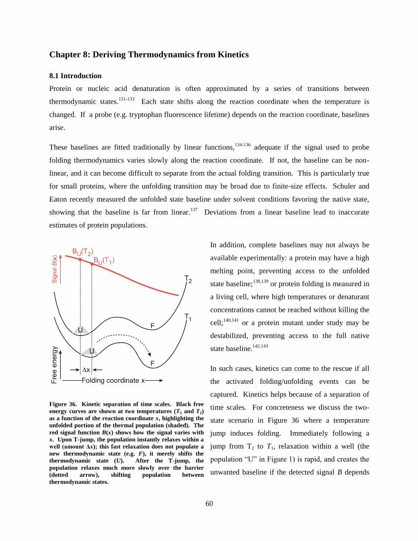
60

Chapter 8: Deriving Thermodynamics from Kinetics

8.1 Introduction

Protein or nucleic acid denaturation is often approximated by a series of transitions between

thermodynamic states.131-133

Each state shifts along the reaction coordinate when the temperature is

changed. If a probe (e.g. tryptophan fluorescence lifetime) depends on the reaction coordinate, baselines

arise.

These baselines are fitted traditionally by linear functions,134-136

adequate if the signal used to probe

folding thermodynamics varies slowly along the reaction coordinate. If not, the baseline can be non-

linear, and it can become difficult to separate from the actual folding transition. This is particularly true

for small proteins, where the unfolding transition may be broad due to finite-size effects. Schuler and

Eaton recently measured the unfolded state baseline under solvent conditions favoring the native state,

showing that the baseline is far from linear.137

Deviations from a linear baseline lead to inaccurate

estimates of protein populations.

In addition, complete baselines may not always be

available experimentally: a protein may have a high

melting point, preventing access to the unfolded

state baseline;138,139

or protein folding is measured in

a living cell, where high temperatures or denaturant

concentrations cannot be reached without killing the

cell;140,141

or a protein mutant under study may be

destabilized, preventing access to the full native

state baseline.142,143

In such cases, kinetics can come to the rescue if all

the activated folding/unfolding events can be

captured. Kinetics helps because of a separation of

time scales. For concreteness we discuss the two-

state scenario in Figure 36 where a temperature

jump induces folding. Immediately following a

jump from T2 to T1, relaxation within a well (the

population ―U‖ in Figure 1) is rapid, and creates the

unwanted baseline if the detected signal B depends

Figure 36. Kinetic separation of time scales. Black free

energy curves are shown at two temperatures (T1 and T2)

as a function of the reaction coordinate x, highlighting the

unfolded portion of the thermal population (shaded). The

red signal function B(x) shows how the signal varies with

x. Upon T-jump, the population instantly relaxes within a

well (amount Δx); this fast relaxation does not populate a

new thermodynamic state (e.g. F), it merely shifts the

thermodynamic state (U). After the T-jump, the

population relaxes much more slowly over the barrier

(dotted arrow), shifting population between

thermodynamic states.

61

on the reaction coordinate x. Relaxation between wells

(dotted arrow ―U‖ to ―F‖ in Figure 1) is slow, and

corresponds to the desired population transfer among

thermodynamic states. If the activation barriers are

large enough, kinetics can separate the fast relaxation

within thermodynamic states from the slow transitions

among thermodynamic states. Thus a small kinetic

jump automatically separates baseline from folding

amplitude, or, when such a separation ceases to exist,

indicates that relaxation in a single well occurs

(downhill folding).144

Here we derive the necessary equations to allow

accurate melting temperatures Tm to be extracted when

baselines are incomplete, non-linear or noisy. We

compare the ‗thermodynamics from kinetics‘ approach

with conventional thermodynamic fitting, showing that

our approach is much more robust when baselines are

incomplete. To do so, we first analyze thermodynamic

and kinetic simulations obtained from the same

microscopic model by solving the Smoluchowski

equation.

8.2 Computational Methods

To compare the ‗kinetics from thermodynamics‘ with

conventional thermodynamic model fits, we simulated

thermodynamic and kinetic data for fitting. A one-

dimensional two-state free energy surface G(x,T) was

modeled as the sum of two Gaussians with the depth of

one well allowed to vary linearly with temperature,

similar to the schematic in Figure 36. The signal function, B(x,T) was modeled as a straight line with a

temperature-dependent y-axis intercept. For the case shown in Figure 38, the temperature-dependence of

the signal function was strictly linear, while in Figure 39, a quadratic component was added to generate

folded and unfolded baselines with opposite slopes.

Figure 37. Comparison of traditional heat

denaturation and „thermodynamics from kinetics.‟

Top: thermodynamic folded baseline, transition and

unfolded baseline. Red labels are defined by the

equations in the text. a, b and c label kinetic T-jumps

shown in Middle: at “a,” little population switches

states, and the resolved phase is small. The instant

phase is proportional to the baseline slope. At “b”, a

large population switch between states is resolved. At

“c,” the resolved phase is small again. The instant

phase has switched sign because the baseline slope has

switched sign. Bottom: By plotting only the resolved

amplitude (solid curve), the baselines are reduced and

only population changes (maximized at b) are selected.

Integrating the amplitude curve yields the

(unnormalized) population as a function of

temperature. The melting point of the protein is easily

identified near the maximum at b, even if the baseline

at a or c cannot be fully measured.

62

The equilibrium populations ρ(x,T) at each temperature were used to determine the thermodynamic

titration signal B(T) (see Equations (36) and (37)). For the kinetic data, 4 degree temperature jumps were

simulated with a final temperature corresponding to each of the points in the thermodynamic titration.

The population change as a function of time was determined from Smoluchowski dynamics using the

singular-value basis method of Chapter 6 and ref. 145

. An exponential decay function was fitted to

determine the resolved amplitude.

To compare the performance of the models with noisy data, equal amounts of Gaussian noise were added

to the thermodynamic melts and kinetic traces. At each noise level, this was repeated with 10 different

sets of random noise, and the models were fitted using 20 pseudo-random initial guesses for the

parameters. The Tms from the best least-squares fit among these initial conditions were averaged to report

the fitted Tm. When fitting the kinetic amplitudes to determine Tm, each point was weighted by the

uncertainty of the resolved amplitude from the exponential fit. When the exponential fit did not converge

or the fitting error was greater than the amplitude, the resolved amplitude was set to 0 and the uncertainty

of the point was set to the RMS noise. An additional point with zero amplitude and low uncertainty was

added 90-100 degrees away from the edges of the data at both high and low temperature.

8.3 Model

The fitting procedure discussed here can be used to improve accuracy for any thermodynamic

perturbation, such as temperature or denaturant concentration. For concreteness, we will consider

temperature as our example. Furthermore, kinetic separation of in-well and barrier-crossing dynamics

improves thermodynamic fitting for two-state or multi-state proteins. Again for concreteness, we

describe the two-state case.

Consider the model represented in Figure 36 and Figure 37. The free energy along the reaction

coordinate (which may also be formulated in more than one dimension145

) leads to a normalized

equilibrium population

. (36)

The free energy and population depend on temperature (the example discussed here). The signal function

B(x) along the reaction coordinate thus yields an observed signal (e.g. tryptophan fluorescence, IR

absorption, FRET, etc.) as a function of temperature

. (37)

63

If the two-state (or n-state) approximation is valid, i.e. if the barriers are high enough, we can divide the

reaction coordinate into states, such as a ―folded‖ and ―unfolded‖ side in the two-state case. The dividing

surface will lie near the barrier.

∫

∫

(38)

The second line is obtained by defining

and accordingly, and setting

and likewise. The observed signal depends on a nonlinear

unfolded baseline weighted by the unfolded population, and a folded baseline weighted by

a folded population.

The populations are related to the free energy by

∑

(39)

and for the two-state case, a simple and frequently used model for the free energy, equilibrium constant,

and population is

.

(40)

The goal is to determine the fitting parameters Tm and g(1)

by extracting ρF(T) from B(T). In particular,

linear baselines with adjustable slopes m have been used in a vast literature to approximate BU(T) and

BF(T).

( ) ( ) (41)

The problem is that if data cannot be collected to map out full baselines, the baseline fitting parameters

Bi0 and mi cannot be determined accurately. Even if the full baseline is observed, it may be steep or

nonlinear in practice, and a linear extrapolation for example of the unfolded baseline into the folded

region (low temperature) is inaccurate or inadequate. This has been demonstrated by single molecule

experiments. The result is that Tm and other fitting parameters cannot be determined accurately.

Kinetics can help out. If kinetics can be measured that capture all well-to-well relaxation events, easily

possible nowadays with nanosecond temperature jumps, the baseline to a significant extent can be

separated from the population change. This is illustrated by Figure 37 a-c: at low or high T where only

in-well relaxation occurs, kinetics mostly shows a sudden jump, due to the baseline. If kinetics are

64

measured near Tm, the well-to-well dynamics produce a resolvable amplitude. At Tm, the resolved

dynamics has the largest amplitude. Plotting the resolved amplitude thus maps out the thermodynamic

transition with a maximum at Tm (Figure 37). This curve can be integrated to yield the population curve.

The key is that a straight thermodynamic fit depends on extrapolation of baselines into the region where

folded and unfolded populations are comparable, whereas kinetics directly determines the difference of

those baselines in that region.

Mathematically, the kinetic signals just before the jump, just after the jump, and at equilibrium, are

(42)

Measuring kinetics independently determines a resolved and an unresolved amplitude

[ ][ ]

[ ] [ ] (43)

or

[ ]

[ ] (44)

Eqs. (44), together with a model for the population ρF such as eq. (40), constitute the kinetic fitting model.

The following should be clear from eq.(44). There are still two baseline functions (here A and C), just as

in the thermodynamic fit in eq. (38). Unlike eq. (38), now two data points at each temperature constrain

the baseline functions and populations, instead of a single data point. Also unlike eq. (38) or eq. (41), the

baseline functions A and C in eq. (44) are difference functions (either between different baselines, or

between a single baseline at two nearby temperatures). Thus A and C are much more likely than the

original baselines to be approximated by linear functions or even constants.

The following are good approximations when a small jump ΔT is applied:

|

(

| ⁄

| ⁄

)

(45)

65

In particular, Bresolved contains a lot of useful information on its own. It is proportional to the derivative of

the thermodynamic population curve. Furthermore, if the folded and unfolded baselines are far apart, or

if they are parallel, then A(T) is approximately or exactly constant, and can be expanded accurately as a

linear baseline. Using the two-state population model in eq. (40) yields

⁄

[ ⁄ ]

( ⁄ ) (46)

with only four fitting parameters g(1)

, Tm, A0, mA, including the last two for the baseline. This model

requires 2 fewer fitting parameters than eqs. (39) and (40), the standard linear baseline two-state fit, and is

expected to yield Tm and g(1)

more reliably.

8.4 Results and Discussion

To compare the standard thermodynamic fitting (eq. (41) combined with the two-state model in eq. (40))

with the ‗thermodynamics from kinetics‘ fitting (eqs. (45) or (46) combined with the two-state model in

eq. (40)), two sets of test data with different baselines were simulated. The model Tm was 323 K in

both cases. The results are summarized in Figure 38 and Figure 39. Panels A and B show the

thermodynamic titration and the resolved kinetic amplitude Bresolved. Figure 38 corresponds to a ‗difficult‘

case very similar to FRET experiments. In

cases like these, a small amount of noise can

make it difficult to identify the cooperative

region. Figure 39 corresponds to an ‗easy‘

case where the folded and unfolded baselines

have different slope, so the transition is

clearly discernible. Regardless of these

differences, we observed similar relative

performance between the thermodynamic and

kinetic models.

Panel C of Figure 38 and Figure 39 shows the

deviation of the melting temperature from the

known value as data points were removed

from the high-temperature unfolded baseline.

This is a common difficulty with in vivo or

living cell experiments, where high

temperature measurements cannot be

Figure 38. Model data derived by Smoluchowski dynamics from a

two state free energy and signal function. The data were chosen to

correspond to a „difficult‟ case, such as FRET with a small

protein. (A) Conventional thermodynamic melt. (B) Resolved

kinetic amplitude. (C) Error in the fitted melting temperature as

function of deleted points in the high temperature baseline. (D)

Combined random and systematic error in the melting

temperature as a function of noise added to the data in (A) and (B)

(same rms noise for both).

66

made.141

The thermodynamic model became

unstable quickly as the baseline was removed.

The kinetics were able to fit Tm reliably until

the peak of the resolved amplitude was

truncated (removal of half of the data points).

Similar results for both models were obtained

by removing the folded baseline, or by

symmetrically removing both baselines

progressively.

Because experiments do not produce infinite

signal to noise, we tested how the

thermodynamic and ‗thermodynamics from

kinetics‘ fits performed with varying amounts

of noise added to the test data. Panel D of

Figure 38 and Figure 39 shows the error in Tm

as a function of noise level. Two sources of

error are included by generating multiple data

sets with different random Gaussian noise. One was the average deviation from the known melting

temperature, and the other was the standard deviation of fit. The error is reported as the square root of the

sum of squares of these two sources of error and is given in the same arbitrary units as the signal shown in

Panels A and B. ‗Thermodynamics from kinetics‘ generally makes smaller errors than a conventional

thermodynamic fit at the same noise level.

The measurement of protein melting temperatures can be a challenge when the high temperature baseline

is missing, or when the baselines are steep. These problems can occur in many situations: Some proteins

aggregate at high concentration, and need to be measured at low concentration. Some proteins have

melting points to close to the boiling point of the solvent. And with an increasing interest in folding in

living cells, or even in vivo, the high temperature baseline may be inaccessible without killing the cell or

organism under study. In such cases, it would be nice to have a method for measuring protein stability

without the need for scanning the whole baseline.

For all of the cases we simulated, we found that the method of fitting ‗thermodynamics from the kinetics‘

was more reliable than conventional thermal melts when baseline information is limited. Kinetics

eliminates most of the baseline by shifting it into the unresolved phase, whereas the population switch

Figure 39. Model data derived by Smoluchowski dynamics

from a two state free energy and signal function. The data were

chosen to correspond to an „easy‟ case, with different slopes for

the folded and unfolded baselines. (A) Conventional

thermodynamic melt. (B) Resolved kinetic amplitude. (C)

Error in the fitted melting temperature as function of deleted

points in the high temperature baseline. (D) Combined random

and systematic error in the melting temperature as a function of

noise added to the data in (A) and (B) (same rms noise for

both).

67

among wells falls into the resolved phase. The latter

yields a nearly baseline-free signal with a peak near Tm,

although large baselines of opposite sign or transitions

occurring over a wide temperature range could shift the

peak somewhat.

The ‗thermodynamics from kinetics‘ model yields a

more consistent increase of the error with baseline

truncation. In Figure 39C, the nonlinearity of the

unfolded baseline leads to a non-monotonic error due to

the non-linear high-T baseline truncation. As further

data is removed however, the unfolded baseline is lost

and the thermodynamic model is unable to fit the

melting temperature. The kinetic fit has a predictably

increasing error when the baseline is truncated, and

generally performs well until the truncation reaches the

denaturation midpoint.

We added the same amount of noise mathematically to

the thermodynamics and the kinetics test data. We also

find that the ‗thermodynamics from kinetics‘ method is

less susceptible to experimental noise. This is due to

the fact that experimental noise is added to a derivative

of the thermodynamic signal (T-jump), rather than

adding the noise to a smooth function and then taking

the derivative. Figure 40 demonstrates one point from the selected data in Figure 38. In the

thermodynamic case, the upper baseline becomes completely washed out and the model fits it such that

the transition region becomes part of the upper baseline. In the kinetic case, however, even when ~1/2 of

the amplitudes have fitting errors larger than the amplitude of the fit and are consequently set to 0, the

peak region can still be easily resolved within a few degrees.

Ironically, the experimentally relevant noise is often worse for the thermodynamic signal than for the

time-resolved kinetic signal, even though the thermodynamic signal is collected over a longer time period

with more signal averaging. In fact, slow data collection amplifies errors such as laser intensity or sample

temperature fluctuations during data collection.

Figure 40. Comparison of noise between

thermodynamic and „thermodynamics from kinetics‟

models. An equal amount of Gaussian noise was

added to the thermodynamic titration and to the raw

kinetic traces from which the resolved amplitudes

were taken. The baselines of the thermodynamics

quickly becomes difficult to resolve, but even with

large fitting errors in the kinetics, a peak is still

resolvable near the melting temperature.

68

The kinetic model can be constrained more easily than the thermodynamic model. For a two-state

system, the resolved kinetic amplitudes approach zero away from the melting temperature; for the

thermodynamics, the baselines have no similarly consistent constraint. Moreover, the slope of the

baseline in the kinetic model can often be constrained to zero, which reduces the fitting parameters to

three. Kiran Girdhar in our lab provided experimental data for the PI3K SH3 domain, which was found

to have very consistent Tm fits for the kinetics under such a constraint.

The major drawback of ‗thermodynamics from kinetics‘ is that all barrier-crossing phases must be

resolved. Otherwise, genuine population transfer is lumped together with dynamics within a single state

in the instant response right after the T-jump (or other relaxation). Thus methods with good time

resolution must be employed for the measurement.

In summary, ‗thermodynamics from kinetics‘ provides simple formulas for fitting the resolved kinetics

amplitude to obtain thermodynamic parameters such as Tm. The result is more robust to truncation of the

baseline and noise than are conventional thermodynamic fits, and the only drawback is that the kinetics

must resolve all barrier crossing events so that the instant amplitude contains only the baseline from

dynamics within states.

69

: Laser Alignment Appendix A

The experimental design for optically-assisted STM experiments requires the coupling of one or more

lasers into the STM. For experiments taking place in the infrared, a minimum of two lasers must be

overlapped for effective laser alignment at the STM. One of these is the laser resonant with the molecular

transition of choice, while the second is a visible laser that will aid in alignment within the vacuum

system, but which will not be active during experiments. For frequency-modulated experiments a third,

non-resonant laser must be overlapped for the minimization of differential heating.

For infrared experiments studying the first electronic transition in single-walled carbon nanotubes, the

resonant laser is a tunable external-cavity diode laser (LiON, Sacher Lasertechnik) capable of producing

radiation from 1165 nm to 1265 nm. The non-resonant laser is a fixed-wavelength diode at 1300 nm.

The visible alignment laser is a helium-neon (HeNe) laser. Figure 41 shows the way in which the optical

table is set up.

The resonant laser is first aligned by adjusting the position of the fiber coupler and the positioning of M1

so that the laser spot is centered on both irises, I1 and I2. The infrared spots are centered with the use of

an infrared detector card (ThorLabs VC-VIS/IR). The HeNe is then centered through the two irises by

adjusting M4 and BS2. With the resonant laser and the HeNe overlapped, the position of the resonant

laser inside the STM UHV chamber can be determined by simple visual inspection. The non-resonant

laser is then centered on the irises using M2 and M3. This results in three collinear propogating beams.

Additionally, the height of the non-resonant laser is chosen such that it passes through the chopper 180°

out of phase with the resonant laser.

To ensure optimal overlap of the beams, a kinematic mount with a mirror is mounted at KM and reflected

off of M7 through a pinhole positioned at X. X is measured to be the same distance from KM as the

STM. The light passes through the pinhole to a power meter and each of the beams is individually

adjusted to maximize the power through the pinhole.

The beam spot size and divergence is measured by placing a set of razor blades on a 3-D micrometer

mount at X. As the razor blades are moved with the micrometers, the 80% / 20% power positions are

monitored with a power meter. L2 is on a translation stage with a micrometer to adjust the focus and

therefore the spot size at X, and consequently, at the STM.

70

Figure 41. Optical setup for frequency-modulated optically-assisted STM experiments. The lenses are f=30 cm UV

lenses; for optimal transmission, IR anti-reflection coated lenses could be substituted. BS1 is a broadband, non-polarizing

beamsplitter cube anti-reflection coated for 1100-1600 nm (Newport 10BC17MB.3). BS2 is a dichroic

mirror/beamsplitter that reflects the HeNe and transmits the IR light efficiently. All of the mirrors are gold-coated. The

position X is measured the same distance as the STM at which point various comparative measurements can be made

when M7 is inserted on a kinematic mount. The power meter at M5 allows the real-time power to be measured

simultaneous with SMA-STM to ensure that power fluctuations do not dominate the signal.

71

: Experimental Procedures Appendix B

Vacuum System

All of our STM experiments are done under ultrahigh vacuum (UHV). Figure 42 shows a schematic of

the vacuum system and the conditions under which valves can be opened during normal system operation.

In addition to the pumps shown in Figure 42, both the prep chamber and the STM chamber have titanium

sublimation pumps (TSP) contained in a cryoshroud. The TSP pumps should be run regularly to maintain

a low background pressure in the chambers and is particularly important in the prep chamber, as it is

subjected to the largest pressure fluctuations. The TSP is operated by filling the cryoshroud with liquid

nitrogen and sputtering titanium onto the cryoshroud walls by applying 45 A of current to one of the TSP

filaments.

Everything loaded into the UHV system must be thoroughly degreased and cleaned and then degassed in

the prep chamber before transfer to the STM. For most samples and many other materials, sonication in

acetone and isopropyl alcohol is a sufficient cleaning procedure. Ceramic parts should be baked in a

furnace after solvent cleaning due to their large surface area and porosity to prevent outgassing. Newly

machined parts tend to have embedded oils and should undergo additional degreasing steps before solvent

cleaning. Metals can be electro-polished, acid cleaned, and degreased in 409.

Degassing is done by resistive heating on the dipstick. When possible, degassing should take place by

resistive heating through the sample or through tip holders in the tip carrier. The dipstick should not

exceed 150 °C and can be cooled with nitrogen while the degas is allowed to heat further locally.

Materials should be heated slowly enough that the prep pressure does not spike much above 1x 10-8

torr.

This heating is done with a DC power supply by passing current through the two terminals in the rotary

stage feedthrough that are opposite each other. For things that cannot be heated directly by resistive

heating, the power supply can be switched to the two terminals labeled ―F‖ on the rotary stage

feedthrough, which will resistively heat a filament inside the dipstick. Materials in good thermal contact

with the dipstick will be heated by indirectly by the filament. Due to the Viton seals in the rotary stage,

this method is restricted to heating to 150 °C.

72

Preparation of wedged Si

Figure 43 shows the geometry of the rear-illumination SMA-STM setup. Total internal reflection at the

sample face must be achieved, which happens when the angle D is greater than the critical angle, which is

given by

(

)

(47)

where n2 is the index of refraction for the vacuum, and n1 is the index of refraction for the silicon. Using

values of 1.000 and 3.559, respectively, the critical angle is 16.3°. Based on the experimental angles of A

and B, angles C and D be derived from trigonometric relationships and Snell‘s law as

(

)

(48)

The other consideration in the choice of angles is the loss of light due to reflection at the wedge itself,

which can be determined from the Fresnel equations, given in Equations (4) and (5). For the current

Figure 42. Schematic of the vacuum system and valves of the UHV-STM. The circles represent inline valves and the solid

rectangles represent VAT gate valves. The normal operational positions of the valves are listed to the right as well as the

parameters under which valves can be opened.

73

optical setup, the wedge is 15° and angle B is 31°, which gives an angle at D as 26.2°, which exceeds the

critical angle for total internal reflection.

We typically machine the wedge at angle A to be ~15°. The machining process involves bonding a

silicon wafer polished side-down onto another sacrificial silicon wafer. Crystalbond 509 (SPI Supplies) is

a wax that is readily soluble in acetone and melts at 121 °C. The scrap wafer is heated on a hot plate and

a stick of Crystalbond is rubbed over the surface to flow on a layer of the wax. The sample wafer of

silicon is then placed face-down on the wax and the wafers are removed from the heat. Using the known

thicknesses of the wafers and by measuring the thickness of the bonded system, the wedge can be diced

on a diamond dicing saw.

Figure 44 demonstrates the way in which the wedge is diced into the wafer. After calibrating the height

of the dicing saw chuck in accordance with the saw‘s operating procedures, the bonded wafers are

adhered to the saw chuck with the integrated vacuum. At a feed rate of 0.25 in/sec at a spindle speed of

17 kRPM, 20 cuts are made 0.002‖ apart to make a clearance area for the laser beam. The wedge is then

cut by reducing the y-spacing to 0.001‖ and creating a stairstep pattern at the desired angle. It is possible

to machine more than one wedge on a 4‖ wafer. The sample is then removed and the wedge is thoroughly

polished with a Dremel using 1 μm alumnia paste and a polishing wheel until the wedge achieves a

smooth, mirror-like finish. The wafers are then returned to the dicing saw and diced into 0.3‖ x 0.2‖

samples that will fit into the STM sample holder. To ensure that the cuts are sufficiently deep enough,

cuts should be made into the sacrificial silicon wafer underneath. The samples can be removed by heating

Figure 43. Laser geometry for experiments on silicon. Angle A is the machined wedge angle. B is the angle at which the

laser is introduced into the STM. C is the incident angle on the wedge and D is the angle at the face of the silicon which

must exceed the critical angle for total internal reflection.

74

the wafers on a hot plate and sliding the samples off. The Crystalbond can be left on the samples until

their use at which point the Crystalbond can be removed with acetone.

Preparation of Si(100)2x1:H

We passivate our silicon samples with hydrogen in situ to create the cleanest possible surface. This

involves loading a clean sample, flashing and annealing the sample in vacuum to create the clean

reconstructed surface, and chemisorbing a monolayer of atomic hydrogen on the surface. We follow the

same passivation procedure described elsewhere,146

though the details of the procedure are relayed here.

The silicon samples are diced based on the procedure described in the previous section. The samples are

thoroughly cleaned of the Crystalbond wax with acetone and then are further cleaned with isopropyl

alcohol. For wedged samples, we avoid sonication to prevent the fragile samples from cracking along the

machined wedge. The silicon samples are handled with Teflon tweezers at all times to avoid nickel

Figure 44. Wedge dicing schematic for silicon. Two silicon wafers are bonded polished sides together with crystal bond

509 wax, then vacuum adhered to a diamond dicing saw chuck and the wedge is machined by dicing stairsteps across the

wafer. After polishing the wafer, the wafers are returned to the dicing saw to cut into pieces that will fit into an STM

sample holder.

75

contamination that might result from the use of stainless steel tweezers. The sample is then put into UV

ozone for ~20 minutes for further cleaning and to create a protective oxide layer that will be removed

during the sample flash. Two pieces of clean 0.25 mm thick 99.997% Ta foil (Alfa Aesar) are folded and

placed over the edges of the sample to improve contact with the sample holder clamps.

The sample holder with the Si sample is loaded into the UHV preparation chamber and degassed on the

dipstick at ~600 °C for ~6 hours. The degas takes place by resistive heating through the silicon sample on

the dipstick by a DC power supply in constant current mode. The sample temperature is monitored with a

pyrometer at an emissivity setting of 0.7. The temperature of the dipstick and the chamber pressure are

monitored during the procedure to ensure that neither goes too high. Because of the Viton seals in the

dipstick rotary stage, the dipstick temperature should stay below 150 °C. To prevent the base pressure of

the prep chamber from rising substantially, the pressure should not readily exceed 1 x 10-8

torr.

During the sample degas, the cracking filament can be briefly degassed for a few seconds at ~18 V from a

Variac. When the sample degas is complete, the degas power is turned off and the dipstick is cooled to

room temperature with nitrogen gas and the flow of gas should be maintained during the flash. To

minimize the background pressure in the prep chamber, the cryoshroud is filled with liquid nitrogen. The

sample is flashed by resistive heating with the DC power supply to ~1200 °C as monitored by the

pyrometer and then slowly cooled (over ~30 seconds) to achieve a 2x1 surface reconstruction on the (100)

surface. If a clean silicon surface is desired, the sample can be moved to the STM chamber at this point.

During passivation, we want to achieve only monohydride formation. At room temperature, only the

dihydride forms, which can lead to etching of the surface, but at ~650 K, only the monohydride is

formed.147

During the sample flash, a temperature vs power relationship can be determined using the

pyrometer and extrapolated to this temperature. In practicality, setting the current between 0.4 and 1.0 A

for wedged silicon samples usually produces excellent surface passivations. The ion pump gate valve is

typically closed during the passivations to improve the lifetime of the pump, though the valve can be left

open during the passivation if adequately clean samples are not routinely produced. The chamber is

backfilled to between 2 and 4 x 10-6

torr with high purity hydrogen from a leak valve on the preparation

chamber from a manifold pressurized to 20 psi. The cracking filament is set to ~12 V to achieve a

temperature of ~1500 K and the sample is passivated for 10 minutes to achieve monolayer adsorption of

hydrogen. After passivation, the leak valve is closed, the gate valve to the ion pump is opened, and the

sample is returned to room temperature. When the base pressure of the prep chamber has recovered, the

sample can be transferred to the STM for scanning.

76

Sample Annealing

Sapphire

To achieve optimal flatness, sapphire substrates should be annealed above 1200 °C.148

We have found,

however, that we achieve suitable flatness by annealing in the tube furnace in the Lyding lab at its

maximum setpoint of 1000 °C. We score the back of the sample in the corner with a diamond scribe

before annealing to make easy the future determination of the sample face. The annealing is performed

by loading the samples on a quartz plate and sliding it into the furnace at the location of the thermocouple

with the furnace at room temperature. Acceptable parameters include using the normal ramp rate of the

furnace, the temperature maintained for several hours at 1000 °C, and passive cooling by allowing the

furnace to slowly air cool.

In situ annealing

Some samples that are prepared ex situ do not produce good imaging under normal degassing conditions

and do not produce high resolution images until after the samples have been annealed in vacuum. One

example of this are the graphene films described in 4.2 . These samples can be annealed by resistive

heating of the sample to several hundred degrees. For samples that cannot support sufficient current for

this type of heating, a silicon backing can be mounted behind the sample and the annealing temperature

can be achieved by resistive heating of the backing. In these cases, the temperature can be monitored

with a pyrometer.

Prism attachment to sapphire samples

Figure 45 shows a schematic of the attachment of a prism to sapphire with an optical epoxy. A number of

different optical epoxies can be used, though these descriptions will involve Epo-Tek 302-3M, which has

an index of refraction n=1.556, which is nearly index-matched to the n=1.51 of the glass prism. For other

epoxies, Snell‘s law can be used to calculate the change through the epoxy. The sapphire has n=1.76.

Using a similar geometric methodology as that presented for the wedge in the silicon, the relevant angles

are given by

(

)

(

)

(49)

77

From Equation (47), the critical angle for total internal reflection is 34.6°. For the current optical setup

with angle A=31°, B is 14°, C is 9.2°, and D is 44°, which exceeds the critical angle. One notable

difference between this experimental design methodology and the silicon platform is that there is

substantially less loss at all polarizations when the light is incident on the prism than on the higher

dielectric material, silicon, as determined by the Fresnel equations.

The easiest way to attach the prism to the samples is after they are already loaded into the sample holder

by applying a bead of the mixed epoxy to the back of the sample while the sample holder is suspended

vertically with the sample facing down. The prism can then be dropped in place. While the epoxy should

cure quickly, the small surface area exposure to the air slows this process and the prism will slide if it is

not properly cured. With the sample holder in the same geometry, it can be placed in a small vacuum

chamber or in a warm furnace to speed the curing process. Once the epoxy is properly cured, the prism

on the sample can be used in the STM and can be safely heated during degas without the prism sliding.

For removal and re-use of the prism, Epo-Tek 302-3M can be dissolved with vigorous soaking in

methylene chloride and this removal process is made easier if the initial bead of epoxy applied is large

enough to provide solvent access to the epoxy.

STM Tip Preparation

STM probes can be easily created by electrochemical etching of tungsten wire in a ―drop-off‖ method.149

Degreased 0.009‖ diameter tungsten wire (Small Parts, Inc.) is held by a set of alligator clips and

suspended vertically through a gold ring held by another set of alligator clips so that the wire drops a few

Figure 45. Total internal reflection geometry for a prism on sapphire. The prism is a right-angle prism and the change in

angles through the epoxy is negligible for Epo-Tek 302-3M because the prism and the epoxy are nearly index matched.

78

mm‘s below the ring. The ring is dipped into a small beaker with 3 M NaOH prepared with ultrapure

deionized water (18 MΩ-cm) to create a meniscus of electrolyte. The gold ring is attached to the cathode

of a DC power supply and the wire is attached to the anode. A bias is applied to etch the wire to a narrow

neck at which point the wire will break and the bottom piece will drop, creating a tip which can be caught

in a micropipette tip with a piece of Kimwipe stuffed into it. The tip can then be picked up with tweezers

and rinsed in a steady stream of deionized water with the tip facing away from the source of the stream.

We have found that drop-off voltages of 3-3.5 V reproducibly create usable tips. The etching process can

be accelerated substantially, however, by using an arbitrarily larger voltage (that will not break the

electrolyte meniscus) until the tip neck is narrow. After that point, the voltage can be reduced to the 3 V

range. Unless a cutoff circuit is employed, the top piece of wire immersed in the electrolyte cannot be

used as a tip because it will be dulled by additional etching after the drop-off.

We have attempted a number of methods for improving the quality of the tips including characterizing

them by Transmission Electron Microscopy (TEM). We have been unable to find a correlation between

the quality of the tip‘s sharpness as it appears in TEM and the STM imaging quality or stability.

Literature that reports great tip production based on TEM, Auger, or other characterization methods

should be viewed with some skepticism unless it provides convincing results that the tips have been used

with superior success as STM probes.

Preparation of Dry Contact Transfer Applicators

The method by which we deposit carbon nanotubes, and which can be used for other materials as well, is

dry contact transfer (DCT). The applicators are simply frayed pieces of fiberglass wire insulation tied to a

tip holder. A piece of fiberglass insulation can be frayed with a razor blade. This piece can then be made

into a loop with the frayed area exposed and tied onto a tip holder with a piece of wire. The set screw can

be removed from the tip holder and the wire passed through the set screw hole. It is important to ensure

that the wire will not impede the ability of the wobble stick fork to pick up the tip holder. After assembly,

the applicator can be sonicated in acetone and isopropyl alcohol, then dried with dry nitrogen.

After assembly and cleaning, the DCT applicator can be loaded with carbon nanotubes by rubbing it

gently against the inside of the CNT container. Previous protocols in our lab dictated repeatedly loading

the applicator and blowing off excess bundles with nitrogen, but this procedure is unnecessary. Some

large bundles will transfer off the applicator, but the majority of transfer will be of isolated CNTs. The

applicators can be loaded with tips in the tip heater and degassed by the same resistive heating procedure

by heating through the tip holders.

79

Deposition by Matrix-Assisted Sublimation

While DCT is an effective method for the deposition of CNTs and other materials such as exfoliated

graphene, it does not work for all nanomaterials. We were unable to deposit PbS quantum dots (QDs)

onto the surface of hydrogen passivated silicon by DCT, so we developed a new method for in situ

deposition of these materials, which we have named Matrix-Assisted Sublimation (MAS).

Thermal sublimation is a technique commonly used for the deposition of C60 onto unpassivated silicon.150

The 4-6 nm PbS infrared absorbing quantum dots (Evidots, Evident Technologies) are too large for

vacuum sublimation. PbS quantum dots were packed into a matrix of C60 and loaded into an alumina

capillary tube which is resistively heated in vacuum and directed toward the sample face on the dipstick.

The alumina tube is wrapped with a wire and attached to the two sides of a sample doser. When the

matrix reaches the sublimation temperature of the C60 (~250 °C), the QDs will be released into the

vacuum. The C60 molecules do not readily physisorb to the H-passivated surface and can only chemisorb

to the surface at the reactive dangling bond sites. The more massive QDs will physisorb to the surface

leaving isolated nanoparticles on the surface for SMA-STM experiments.

Figure 46. Si:H(2x1) surface after sublimation of 5.3 nm PbS quantum dots in a matrix of C60. STM topographs in (a)

and (b). Inset in (a) shows height on the order of that expected for the QDs. AFM topograph in (c) with highlighted cross-

section in (d). The surface appears to be completely saturated with quantum dots and no apparent features are small

enough to be C60.

80

Figure 46(a) and (b) show STM topographs after sublimation deposition. Figure 46(c) shows an AFM

image that also shows the surface saturated with spherical particles of the expected diameter of the QDs

as indicated by the cross-section in Figure 46(d). This proof-of-concept experiment shows that MAS is a

feasible approach to QD deposition

Additional characterization of deposition parameters will be required to ensure that the surface is not

over-saturated with QDs. This will likely require a DC power supply that is more precise than our 100

mA precision supply. Because C60 sublimes at ~250 °C and the PbS QDs decompose at ~300 °C,

accurate calibration of the molecular doser‘s resistive heating element will be necessary. While it is

possible to deposit isolated QDs on H-passivated Si for STM study using pulse valve injection,151

the

matrix-assisted sublimation will be a much cheaper process that requires no modifications to our UHV

system. This technique could prove useful not only for depositing quantum dots, but it may also be

applicable to other molecules too large for sublimation for which DCT is not effective.

Elevated Temperature Deposition of Metal Films

The heater design for elevated temperature deposition is described in 4.1 . When loading it into the CHA

evaporator in the MNTL cleanroom, the rotatable wafer holder must be moved out of the way of the steel

plate. This can be achieved by setting the sample rotation switch to fixed and choosing an arbitrary

number, then flipping the switch to the ―off‖ position when the sample rotation bar is horizontal. When

facing the front of the evaporator, the wires should be run down the right side of the supports inside the

vacuum chamber to the feedthrough and the four wires clipped onto the feedthrough connections. If the

wires on the ambient side of the feedthrough are not visible, the cabinet cover can be removed to retrieve

them. It is important that when the cover is replaced, the interlock switches are properly pressed or the

―CAB‖ interlock will not light when the e-beam power is turned on and the e-beam will not activate. A

DC power supply and thermocouple reader can then be attached to the four wires after checking that there

are no shorts and that the heater resistance reads 0.8 Ω.

Because the heater resistance is temperature-dependent, we use the DC power supply in constant-current

mode. As the heater increases in temperature, the voltage will increase substantially. The applied current

should be increased and decreased by slowly turning the power supply knob and not exceeding 3 A of

current. Before turning on the mains power to the DC power supply, it is important to check that the

current knob is set to zero and did not get rotated during transportation.

Deposition should be performed per the instructions and training provided for the CHA evaporator by the

MNTL Cleanroom staff. All films shown in Chapter 4 were deposited between 0.6 Å/sec and 1.0 Å/sec.

The power should be ramped up carefully when melting any metal, but particularly with Pt and Nb

81

because they have extremely high melting points. If the power is increased too quickly, the source will

spit off chunks of metal or if the e-beam is slightly misaligned, the crucible can be melted. They should

also be cooled slowly to avoid cracking the crucible. Also of note, Nb is incompatible with normal

graphite crucibles and a Fabmate crucible should be used to avoid melting the crucible when the Nb wets

to the crucible.

82

: Matlab Code for STS Spectra Maps Appendix C

Spectra_Map.m

% spectra_map.m % % Plots a spectra map from a line of spectroscopy points dumped to a text % file from STM software. You must delete the top line of the exported % file that says V I(A) vs V, etc. % % Note that the colorbar is really 10^value % % Gregory E. Scott % 10/22/2008 % Input information pathi=['C:\TEMP\']; %input file path patho=['c:\temp\']; %output file path filei=['11_29_10.sts.TXT']; % name of file containing spectroscopy points fileo=['11_29_10.sts.png']; % name of file for output image points = 40; % number of spectroscopy points spacing = 10; % distance between points in Angstroms % Piece together filenames namer=[pathi,filei]; nameo=[patho,fileo]; % Map Creation X=zeros([1 points]); %Create X values for relative spacing between spectroscopy points converted to nm for n=1:points X(1,n)=(n-1)*spacing/10; end; fid=fopen(namer, 'r'); YZ = fscanf(fid, '%e', [points+1 1000]); % Import I and V fclose (fid); Y=YZ(1,:); % Set voltages as Y values YZ(1,:) = []; % Discard voltages from matrix Z=YZ'; % Transpose matrix and set currents as Z values SMap=surf(X,Y,log10(Z)); % Plot spectra map view(2); shading interp; colormap(jet); set(gca,'XLim',[0 (points-1)/10*spacing]); set(get(gca,'xlabel'),'String','Relative Position (nm)'); set(get(gca,'xlabel'),'FontSize',18); set(get(gca,'ylabel'),'String','Voltage (V)'); set(get(gca,'ylabel'),'FontSize',18); set(gca,'FontSize',18); cb=colorbar;

83

set(get(cb,'xlabel'),'String','I(A)'); set(get(cb,'ylabel'),'String','10','Rotation',0); set(get(cb,'xlabel'),'FontSize',18); set(get(cb,'ylabel'),'FontSize',18); set(cb,'FontSize',18); saveas(gcf,nameo,'png');

84

: Fitting Parameters for PTB1:4W Appendix D

Potential surfaces were encoded as a sum of Gaussian dimples of variable depth Ai(T), variable

anisotropic width σi(T) and position xi(T). For the 1-D there-well surface in Figure 35,

∑ ( )

(50)

The temperature dependence of the parameters Pi in (50) was expanded in a Taylor series to first order,

with a reference temperature T0 of 20 °C:

(51)

Because only the relative well-depths and the barriers between wells are physically significant, we

restricted the Gaussian wells to a minimum depth such that the normalized probability density approached

zero at the edges of the sampling grid. In Figure 35, the depth is offset so that the native well has a

minimum at zero energy. We kept the diffusion coefficient coordinate-independent, but allowed its

average value to vary.

Signal functions Si(x) were chosen to be sigmoids with offset S0, height h, width σ, slope m, and switching

position x0.

(52)

Signal functions shown in Figure 35 were normalized to the range 0 to 1 from the fitted values.

85

Table 1 gives the minimum and maximum values allowed in the genetic algorithm for the final

optimization resulting in the fit presented in 7.3 Initial guesses were determined using larger ranges by

optimizing one set of signal data a time with double-well potentials. Parameter ranges were alternately

constrained to narrow the parameter space until acceptable optimization was realized.

86

Table 1.

Parameter Minimum Maximum Optimized Value

Well 1 A0 50 50 50

dA 0 0 0

σ0 0.3520 0.4850 0.3921

dσ 0 0 0

x0 1.4200 1.4200 1.4200

Dx 0 0 0

Well 2 A0 27.0000 34.0000 29.8018

dA 0.5000 0.6500 0.5600

σ0 0.5060 0.5650 0.5638

dσ 0 0 0

x0 1.8900 2.0700 2.0141

dx 0 0.0026 0.0010

Well 3 A0 42.0000 46.0000 42.8055

dA 0.2000 0.6000 0.3119

σ0 0.5286 0.6390 0.6153

dσ 0 0 0

x0 3.0000 3.1700 3.0496

dx -0.0044 0 -0.00145

Flourescence

Intensity Signal

S0 15 15 15

m 0 4.5400 0.6129

σ 0.00001 0.0440 0.0130

x0 1.2330 1.7620 1.3283

h -15.0000 0 -12.4829

CD Signal S0 25.0000 25.0000 25.0000

m -13.6200 0 -6.1562

σ 0.00001 0.0440 0.0108

x0 2.2030 3.0840 2.8193

h -25.0000 0 -24.0662

Flourescence

Wavelength Signal

S0 25.0000 25.0000 25.0000

m 0 22.7000 11.7064

σ 0.00001 0.0661 0.0141

x0 1.1000 1.7621 1.3933

h -25.0000 0 -11.0785

Diffusion

Coefficient

(nm2/ns)

D 8.8 x 10-6

1.76 x 10-5

1.23 x 10-5

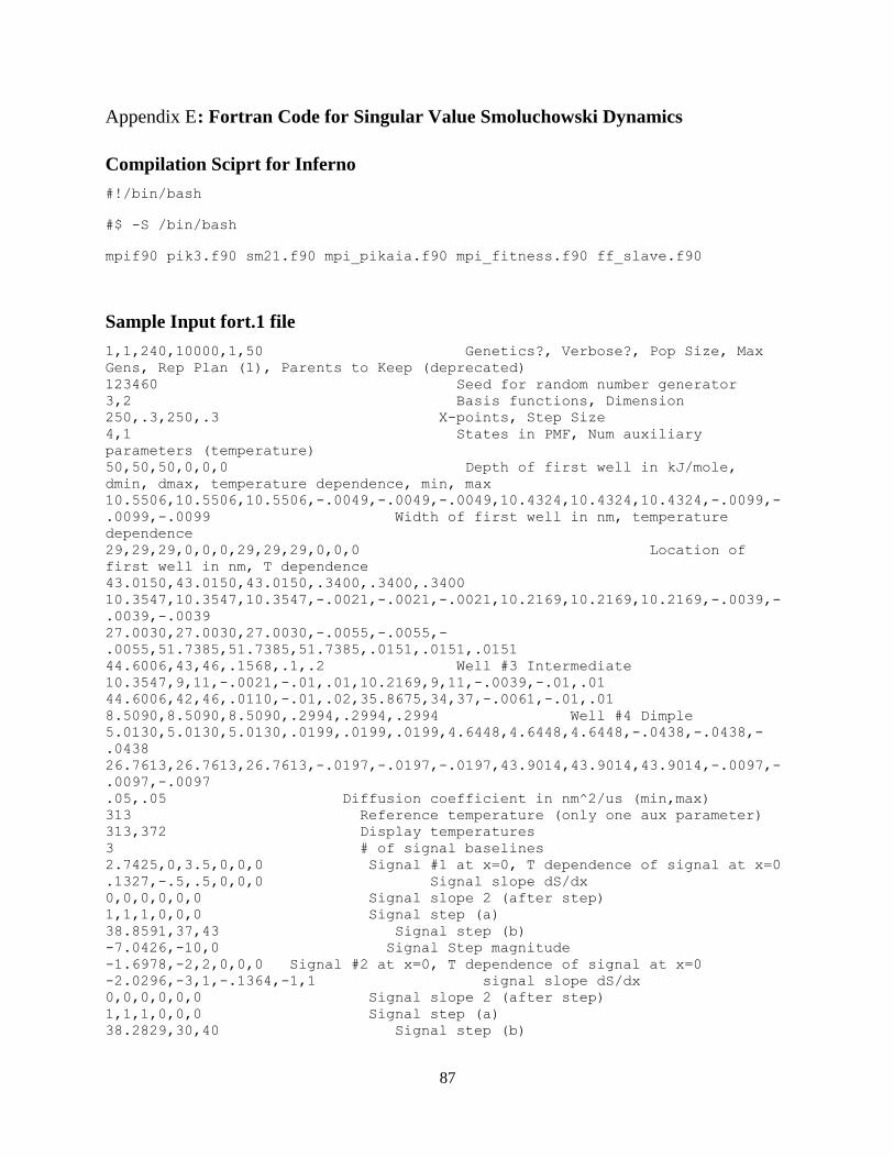
87

: Fortran Code for Singular Value Smoluchowski Dynamics Appendix E

Compilation Sciprt for Inferno

#!/bin/bash

#$ -S /bin/bash

mpif90 pik3.f90 sm21.f90 mpi_pikaia.f90 mpi_fitness.f90 ff_slave.f90

Sample Input fort.1 file

1,1,240,10000,1,50 Genetics?, Verbose?, Pop Size, Max

Gens, Rep Plan (1), Parents to Keep (deprecated)

123460 Seed for random number generator

3,2 Basis functions, Dimension

250,.3,250,.3 X-points, Step Size

4,1 States in PMF, Num auxiliary

parameters (temperature)

50,50,50,0,0,0 Depth of first well in kJ/mole,

dmin, dmax, temperature dependence, min, max

10.5506,10.5506,10.5506,-.0049,-.0049,-.0049,10.4324,10.4324,10.4324,-.0099,-

.0099,-.0099 Width of first well in nm, temperature

dependence

29,29,29,0,0,0,29,29,29,0,0,0 Location of

first well in nm, T dependence

43.0150,43.0150,43.0150,.3400,.3400,.3400

10.3547,10.3547,10.3547,-.0021,-.0021,-.0021,10.2169,10.2169,10.2169,-.0039,-

.0039,-.0039

27.0030,27.0030,27.0030,-.0055,-.0055,-

.0055,51.7385,51.7385,51.7385,.0151,.0151,.0151

44.6006,43,46,.1568,.1,.2 Well #3 Intermediate

10.3547,9,11,-.0021,-.01,.01,10.2169,9,11,-.0039,-.01,.01

44.6006,42,46,.0110,-.01,.02,35.8675,34,37,-.0061,-.01,.01

8.5090,8.5090,8.5090,.2994,.2994,.2994 Well #4 Dimple

5.0130,5.0130,5.0130,.0199,.0199,.0199,4.6448,4.6448,4.6448,-.0438,-.0438,-

.0438

26.7613,26.7613,26.7613,-.0197,-.0197,-.0197,43.9014,43.9014,43.9014,-.0097,-

.0097,-.0097

.05,.05 Diffusion coefficient in nm^2/us (min,max)

313 Reference temperature (only one aux parameter)

313,372 Display temperatures

3 # of signal baselines

2.7425,0,3.5,0,0,0 Signal #1 at x=0, T dependence of signal at x=0

.1327,-.5,.5,0,0,0 Signal slope dS/dx

0,0,0,0,0,0 Signal slope 2 (after step)

1,1,1,0,0,0 Signal step (a)

38.8591,37,43 Signal step (b)

-7.0426,-10,0 Signal Step magnitude

-1.6978,-2,2,0,0,0 Signal #2 at x=0, T dependence of signal at x=0

-2.0296,-3,1,-.1364,-1,1 signal slope dS/dx

0,0,0,0,0,0 Signal slope 2 (after step)

1,1,1,0,0,0 Signal step (a)

38.2829,30,40 Signal step (b)

88

-16.1670,-30,-10 Signal Step Magnitude

2.15,-3.5,3,0,0,0 Signal #3 at x=0, T dependence of signal at x=0

-.5,-1,1,-.0955,-1,1 signal slope dS/dx

0,0,0,0,0,0 Signal slope 2 (after step)

0,0,0,1,1,1 Signal step (a)

38.2,28,47 Signal step (b)

27,0,35 Signal Step Magnitude

0 # Linked Parameters

6 # Data Blocks

0,14,3 datatype=0 means thermo, not kinetics, 13 data

points, use signal #3

1,0,1 scale data?, scalemin,scalemax

100 number of time steps (deprecated)

275.35 1 0.001 275.35 IR at 1660 cm-1

283.05 0.98701 0.001 283.05

289.78 0.94805 0.001 289.78

296.87 0.93506 0.001 296.87

303.15 0.8961 0.001303.15

310.85 0.84416 0.001 310.85

324.85 0.74026 0.001 324.85

331.85 0.64935 0.001 331.85

338.75 0.54546 0.001 338.75

341.85 0.42857 0.001 341.85

345.65 0.32468 0.001 345.65

349.35 0.22078 0.001 349.35

353.15 0.1039 0.001353.15

358.95 0 0.001 358.95

1,9,3 IR 325 K datatype=1 means kinetics, # data points,

Signal #

1,0,1 scale data?, scalemin,scalemax

100 number of time steps

0 1 0.001 315

1000 .69837 0.001 325

2000 .48773 0.001 325

3000 .34062 0.001 325

6000 .11602 0.001 325

12000 .01346 0.001 325

30000 .00002 0.001 325

40000 0 0.001 325

50000 0 0.001 325

1,9,3 IR 343 K datatype=1 means kinetics, # data points,

Signal #

1,0,1 scale data?, scalemin,scalemax

100 number of time steps

0 1 0.001 333

1000 .66564 0.001 343

2000 .44308 0.001 343

3000 .29494 0.001 343

6000 .08699 0.001 343

12000 .00757 0.001 343

30000 0 0.001 343

40000 0 0.001 343

50000 0 0.001 343

0,18,1 datatype=0 means thermo, not kinetics, 61 data

points, use signal #1

1,.0178,1 scale data?, scalemin,scalemax

89

100 number of time steps per observed time

interval to converge propagation

313.15 0.974089 0.001 313.15 T (K), 280 nm fluoresence, uncertainty, T is

only aux parameter

314.15 1 0.001 314.15

316.15 0.963765 0.001 316.15

318.15 0.955364 0.001 318.15

322.15 0.936336 0.001 322.15

326.15 0.923684 0.001 326.15

330.15 0.890891 0.001 330.15

334.15 0.860628 0.001 334.15

338.15 0.789372 0.001 338.15

342.15 0.702632 0.001 342.15

346.15 0.593219 0.001 346.15

350.15 0.488158 0.001 350.15

354.15 0.381275 0.001 354.15

358.15 0.299393 0.001 358.15

362.15 0.201619 0.001 362.15

366.15 0.10668 0.001 366.15

370.15 0.0589069 0.001 370.15

372.15 0.0178138 0.001 372.15

1,9,2 fl 53 oC datatype=1 means kinetics, # data

points, Signal #

1,0,1 scale, scalemin,scalemax

100 number of time steps

0 1 0.001 318

1000 .63474 0.001 326

2000 .40289 0.001 326

3000 .25573 0.001 326

6000 .0654 0.001 326

12000 .00428 0.001 326

30000 0 0.001 326

40000 0 0.001 326

50000 0 0.001 326

1,9,2 fl 71 oC datatype=1 means kinetics, # data

points, Signal #

1,0,1 scale data?, scalemin,scalemax

100 number of time steps

0 1 0.001 336

1000 .8702 0.001 344

2000 .75723 0.001 344

3000 .65891 0.001 344

6000 .43405 0.001 344

12000 .18809 0.001 344

30000 .01455 0.001 344

40000 .0029 0.001 344

50000 0 0.001 344

sm21.f90

! 1- or 2-D dicrete Smoluchowski solver. This program

! propagates a density matrix rho in coordinate space on a

! potential surface pmf. PMF can depend on time via a bias(t)

! parameter. rho(t=0) can be any function, or can be the

! stationary state of pmf[bias(t=0)]. The propagation uses

! singular value decomposition of rho over the range of biases

! encountered to create an orthogonal basis for rho, then

90

! solves the time propagation in this orthogonal basis. For

! small jumps of PMF[bias(t)], even two basis functions are

! sufficient, greatly reducing computational cost for

! calculations of relaxation experiments. To do the SVD,

! subroutine SVDCMP produces a singular value decomposition

! of matrix rho = a * v * w, where v is the basis function

! matrix, w the singular value array, and a the matrix which

! expresses the density in terms of the SVD basis functions.

module set_kinds

implicit none

integer, parameter :: ik=4

integer, parameter :: rk=8

end module set_kinds

module constants

use set_kinds

implicit none

real(rk) :: kb = 0.00831 !! in kJ/mole/K

end module constants

module masterdim

use set_kinds

implicit none

integer(ik), parameter :: rhodim(2)=255,mdim=1000, &

ndim=10,statedim=10,sigdim=6

integer(ik), parameter :: dim=rhodim(1)*rhodim(2)

integer(ik), parameter :: odim=1200, padim=100, &

blockdim=12, auxdim=4, xdim=2, parmdim=65 !Auxillary (eg T)

parameters, dimensions, adjustable parameters

integer(ik), parameter ::

refdim=statedim*auxdim*(1+xdim)+sigdim*(1+auxdim+xdim),linkdim=10,&

numdim=9+xdim*3+auxdim+7*blockdim+2*linkdim

end module masterdim

module obscalc

use set_kinds

use masterdim

implicit none

real(rk) :: xobs(odim),obs(odim),osig(odim),xaux(odim,auxdim)

real(rk) :: calc(odim)

real(rk) :: pa(padim),pasig(padim)

integer(ik) :: onum, panum, paf(padim),linknum, links(linkdim,linkdim)

! The following are independent variables or other

! information required by cal to evaluate calc():

integer(ik) :: statenum, contot, datablocks, scaleflag(blockdim),&

datatype(blockdim), onu(blockdim), datanorm(blockdim), &

sigtype(blockdim),basenum,popu,dat,auxnum, &

tstepnum(blockdim), verbflag, maxgens, genflag, replan, nindv,keepnum

real(rk) ::

datamin(blockdim),datamax(blockdim),scalemin(blockdim),scalemax(blockdim)

end module obscalc

module rhopmfsig

use set_kinds

use masterdim

91

implicit none

real(rk) :: delx(xdim)

real(rk) :: d0(statedim,0:auxdim), dmin(statedim,0:auxdim), &

dmax(statedim,0:auxdim),w0(statedim,0:auxdim,xdim), &

wmin(statedim,0:auxdim,xdim),wmax(statedim,0:auxdim,xdim), &

x0(statedim,0:auxdim,xdim),xmin(statedim,0:auxdim,xdim), &

xmax(statedim,0:auxdim,xdim),aux0(auxdim)

real(rk) :: s0(sigdim,0:auxdim), s0min(sigdim,0:auxdim), &

s0max(sigdim,0:auxdim), s1(sigdim,0:auxdim), s1min(sigdim,0:auxdim), &

s1max(sigdim,0:auxdim),amin(sigdim,0:auxdim),amax(sigdim,0:auxdim),&

a(sigdim,0:auxdim),

b(sigdim),bmax(sigdim),bmin(sigdim),sigstep(sigdim),&

sigstepmin(sigdim),sigstepmax(sigdim),

s2(sigdim,0:auxdim),s2min(sigdim,0:auxdim),&

s2max(sigdim,0:auxdim)

real(rk) :: dc(xdim), dcmin(xdim), dcmax(xdim)

integer(ik) :: nrho,dimen,mpts(xdim),signum, seedset

real(rk) :: basis(dim,ndim), gs(ndim,ndim), svs(ndim),

t1,t2,nums(numdim),&

parmref(refdim,2),disptemp(2),penaltyflag,

rhox(0:rhodim(1)+1,0:rhodim(2)+1)

end module rhopmfsig

subroutine se

!-----------------------------------------------------------------------

! Main program subroutine

! Reads in all input information from file

! Starts genetic algorithm

! Writes all output to files

! Output files:

! pmfrho.out x,y,z coordinates of pmf, rho, and signal functions at ref.

temp

! pmfrho1.out pmf, rho at first specified temperature (aux parameter)

! pmfrho2.out pmf, rho at second specified temperature

! sigs.out Observed (from input file) vs calculated signals

! parms.out PMF and signal function parameters for best fit

!-----------------------------------------------------------------------

use set_kinds

use masterdim

use obscalc

use rhopmfsig

implicit none

integer(ik) :: i1,i2,i3,i3end,i,j,k,l,maxo

character(3) :: datastring,datastring2

real(rk) :: fit, test,test2

real(rk) :: rho(0:rhodim(1)+1,0:rhodim(2)+1), &

pmf(0:rhodim(1)+1,0:rhodim(2)+1), aux(auxdim), &

sigx(0:rhodim(1),0:rhodim(2)),sigxs(sigdim,0:rhodim(1),0:rhodim(2))

! Read spatial grid variables; to allow derivatives to be taken, the

grid

! runs from 0...mpts+1, but only 1...mpts is reported

! nrho # of rho basis functions to be used (minimum of 2!)

! dimen either 1 or 2 spatial dimensions

! m SVD column dimensions (product of mpts in each

dimension)

92

! delx step size in Angstroms

!--------------------Read in all input information---------------------------

-

! First line: do genetics?, verbose?, population size, max generations,

replacement plan

! Replacement plan should be 1 (full generational replacement) for parallel

operation

!----------------------------------------------------------------------------

-

open(unit=1,file='fort.1')

read(1,*) genflag,verbflag, nindv,maxgens,replan,keepnum !keepnum

deprecated

read(1,*) seedset !Random

number seed

read(1,*) nrho,dimen !Number

of basis functions, dimension

read(1,*) (mpts(j), delx(j), j=1,dimen) !Number

of points in each dimension

if (dimen == 1) then

mpts(2)=0

delx(2)=0

else if(dimen == 2) then

print *,"Dimen=2"

endif

! Read PMF Gaussian fitting parameters of each state on the PMF

read(1,*) statenum,auxnum !Number

of states, number of auxillary parameters

do k=1,statenum

read(1,*) (d0(k,i),dmin(k,i),dmax(k,i), i=0,auxnum)

!Well depth

read(1,*) ((w0(k,i,j),wmin(k,i,j),wmax(k,i,j), i=0,auxnum),

j=1,dimen) !Well width

read(1,*) ((x0(k,i,j),xmin(k,i,j),xmax(k,i,j), i=0,auxnum),

j=1,dimen) !Well position

enddo

! Read diffusion coefficient scaling factor and reference values of

auxiliary parameters

read(1,*) (dc(j), dcmin(j), dcmax(j),j=1,dimen)

if(dimen == 1) then

dc(2)=0

dcmin(2)=0

dcmax(2)=0

endif

do i=1,auxnum

read(1,*) aux0(i)

enddo

read(1,*) disptemp(1),disptemp(2) !Temperatures for output of

potentials in pmfrho1.out and pmfrho2.out

! Read signal parameters

read(1,*) signum

do l=1,signum

read(1,*) (s0(l,i),s0min(l,i),s0max(l,i), i=0,auxnum)

read(1,*) (s1(l,j),s1min(l,j),s1max(l,j), j=1,dimen)

read(1,*) (s2(l,j),s2min(l,j),s2max(l,j), j=1,dimen)

93

read(1,*) (a(l,j),amin(l,j),amax(l,j), j=1,dimen)

read(1,*) b(l),bmin(l),bmax(l)

read(1,*) sigstep(l),sigstepmin(l),sigstepmax(l)

enddo

! Read linked parameters

read(1,*) linknum

print *,"linknum:",linknum

do i1=1,linknum

read(1,*) links(i1,1),links(i1,2)

print *,"links:",links(i1,1),links(i1,2)

enddo

! Read observable blocks

read(1,*) datablocks

onum=1

do i1=1,datablocks

read(1,*) datatype(i1),onu(i1),sigtype(i1)

read(1,*) scaleflag(i1),scalemin(i1),scalemax(i1)

read(1,*) tstepnum(i1)

do i2=onum,onum+onu(i1)-1

read(1,*) xobs(i2),obs(i2),osig(i2),(xaux(i2,i3),i3=1,auxnum)

enddo

onum=onum+onu(i1)

enddo

onum=onum-1

!-------------------End Input-------------------------------

!! Start genetic algorithm

call genetic(fit)

!-----------------Output all information---------------------

! Get pmf, rho, and sigx at reference temperature/parameters

do i=1,auxnum

aux(i)=aux0(i)

enddo

call get_pmf(aux,pmf,0,0)

call get_rho(pmf,aux,rho)

do i1=1,signum

call get_sigx(i1,rho,sigx,aux)

sigxs(i1,:,:)=sigx(:,:)

enddo

!! Write pmf and rho to file

open(unit=2,file='pmfrho.out')

i3end=0

if(dimen==2) then

i3end=mpts(2)+1

endif

write(datastring,'(i2)') signum

write(2,*) "xpos ypos pmf rho sig"

do i2=0,mpts(1)+1

94

do i3=0,i3end

write(2,'(2(f6.2,1x),f14.10,1x,f14.10

,1x,'//datastring//'(f8.3,1x))') delx(1)*i2, &

delx(2)*i3, pmf(i2,i3), rho(i2,i3), (sigxs(i1,i2,i3),i1=1,signum)

enddo

enddo

!-------Test----- Project 2-D into 1-D

! open(unit=30,file='slice.out')

! if(dimen==2) then

! test=floor(x0(1,0,1)/delx(1))

! test=floor(x0(1,0,2)/delx(1))

! do i2=0,mpts(2)+1

! write(30,'(f5.2,1x,2(f14.10,1x))'), i2*delx(1),pmf(test,i2)

! write(30,'(f5.2,1x,2(f14.10,1x))'), i2*delx(1),pmf(i2,test)

! enddo

! endif

! do i2=0,mpts(1)+1

! test=0

! do i3=0,i3end

! test=test+rho(i2,i3)*delx(2) !x-slice

! test2=test2+rho(i3,i2) !y-slice

! enddo

! write(30,'(2(f5.2,1x),2(f14.10,1x))') delx(1)*i2,delx(2)*i3,test,test2

! enddo

!----End Test----

!-------------Print pmf/rho at display temperatures-----------------

!!Only works for 1 aux parameter

aux(1)=disptemp(1)

call get_pmf(aux,pmf,0,0)

call get_rho(pmf,aux,rho)

!! Write pmf and rho to file

open(unit=20,file='pmfrho1.out')

i3end=0

if(dimen==2) then

i3end=mpts(2)+1

endif

write(20,*) "xpos ypos pmf rho"

do i2=0,mpts(1)+1

do i3=0,i3end

write(20,'(2(f6.2,1x),f6.1,1x,f6.4)') delx(1)*i2, &

delx(2)*i3, pmf(i2,i3), rho(i2,i3)

enddo

enddo

aux(1)=disptemp(2)

call get_pmf(aux,pmf,0,0)

call get_rho(pmf,aux,rho)

!! Write pmf and rho to file

open(unit=21,file='pmfrho2.out')

i3end=0

95

if(dimen==2) then

i3end=mpts(2)+1

endif

write(21,*) "xpos ypos pmf rho"

do i2=0,mpts(1)+1

do i3=0,i3end

write(21,'(2(f6.2,1x),f6.1,1x,f6.4)') delx(1)*i2, &

delx(2)*i3, pmf(i2,i3), rho(i2,i3)

enddo

enddo

!-------------------------------------------------------------------

!---------------Output parameters of best fit-----------------------

open(unit=5,file='parms.out')

write(datastring,'(i3)') auxnum+1

write(datastring2,'(i3)') auxnum*dimen+1

write (5,'(A,f7.3,A,f6.3)') "Fitness: ", fit, " Sum of squares:

",1/fit

do k=1,statenum

write(5,'(A,i3,A,'//datastring//'(f7.4,1x))') "d0(",k,"):",(d0(k,i),

i=0,auxnum)

write(5,'(A,i3,A,'//datastring2//'(f7.4,1x))')

"w0(",k,"):",((w0(k,i,j), i=0,auxnum), j=1,dimen)

write(5,'(A,i3,A,'//datastring2//'(f7.4,1x))')

"x0(",k,"):",((x0(k,i,j), i=0,auxnum), j=1,dimen)

enddo

write(datastring2,'(i3)') dimen

write(5,'(A,i3,A,'//datastring2//'(f10.6,1x))')

"dc(",j,"):",(dc(j),j=1,dimen)

do l=1,signum

write(5,'(A,i3,A,'//datastring//'(f7.4,1x))') "s0(",l,"):",(s0(l,i),

i=0,auxnum)

write(5,'(A,i3,A,'//datastring2//'(f7.4,1x))')

"s1(",l,"):",(s1(l,j), j=1,dimen)

write(5,'(A,i3,A,'//datastring2//'(f7.4,1x))')

"s2(",l,"):",(s2(l,j), j=1,dimen)

write(5,'(A,i3,A,'//datastring2//'(f7.4,1x))') "a(",l,"):",(a(l,j),

j=1,dimen)

write(5,'(A,i3,A,f8.4)') "b(",l,"):",b(l)

write(5,'(A,i3,A,f8.4)') "sigstep(",l,"):",sigstep(l)

enddo

! Write observed vs calculated data

open(unit=10,file="sigs.out")

write(10,*) " Observed | Calculated"

onum=1

do i1=1,datablocks

write(10,*) "Data Block #",i1

! do i2=1,onu(i1)

do i2=onum,onum+onu(i1)-1

write(10,'(3(f12.4,1x))') xobs(i2),obs(i2),calc(i2)

96

enddo

onum=onum+onu(i1)

enddo

onum=onum-1

end subroutine se

subroutine genetic(fit)

!-----------------------------------------------------------------------

! Routine to set up and start genetic algorithm

!-----------------------------------------------------------------------

use set_kinds

use masterdim

use obscalc

use rhopmfsig

use Genetic_Algorithm

implicit none

integer(ik) :: i,j,k,l,i1,seed,status

integer :: nparms

real(rk) :: fit

real(8) :: ctrl(13), parms(parmdim), fness

INTERFACE

FUNCTION get_fitness(nparms, parms) RESULT(fn_val)

IMPLICIT NONE

INTEGER, INTENT(IN) :: nparms

real(8), INTENT(IN) :: parms(:)

real(8) :: fn_val

END FUNCTION get_fitness

END INTERFACE

! Build linear array of all adjustable parameters in range [0,1]

call scaledownparms(parms,nparms)

! Start the random number generator

seed=seedset

call rninit(seed)

! Set control variables

ctrl(1:13) = -1 !Set everything to default values

ctrl(1)=nindv !Individuals

ctrl(2)=maxgens !Generations

ctrl(3)=6 !Number of digits in chromosome

ctrl(10)=replan !Replacement plan (Must be 1 for

parallel operation)

ctrl(12)=0 !Turn off verbose output

ctrl(13)=keepnum !Deprecated

if(verbflag==1) ctrl(12)=2 !maximum verbose (print fitnesses

every generation)

! Start genetic algorithm

if(genflag==1) then

call pikaia(get_fitness, nparms, ctrl, parms, fness, status)

else

97

fness=get_fitness(nparms,parms)

print *, "No Genetics, Fitness: ",fness

endif

fit=fness

call scaleparms(parms) !Make sure all values are scaled back to

actual ranges

genflag=0 !Turn off genetics flag so output in final

call to cal will be printed

call cal !Run through everything with the most fit

individual

end subroutine genetic

function get_fitness(nparms,parms) RESULT(fn_val)

!-----------------------------------------------------------------------

! This evaluates the fitness of the individual by comparing all calculated

! signals to the observed values from the input file. It is a weighted

! sum of squares. The reciprocal value is used since pikaia evolves to

! higher fitness values.

!-----------------------------------------------------------------------

use set_kinds

use masterdim

use obscalc

use rhopmfsig

implicit none

integer(ik) :: i1,i2

integer, intent(in) :: nparms

real(8), intent(in) :: parms(:)

real(8) :: fn_val, fit

!Rescale from [0,1] to [min,max] for each parameter

call scaleparms(parms)

!Turn the parameters into pmf->rho->signal

call cal

!! Sum of squares fitness

fit = 0

do i2=1,onum

! fit = fit + (obs(i2)-calc(i2))**2

fit = fit + ( (obs(i2)-calc(i2))/osig(i2) )**2 !Now weight

depending on significance

enddo

if(penaltyflag==1) fit=10000 !Apply penalty function if necessary

(flag turned on if rho does not maintain normalization)

fn_val=1/fit !Pikaia only finds max values, so

fitness must increase with decreasing error

end function get_fitness

98

subroutine scaledownparms(parms,nparms)

!---------------------------------------------------------------------------

!Scale values from [min,max] to [0,1] for pikaia input

!Count number of parms and wrap up parameters for parallel sending via MPI

!Parms: Array of only parameters to be evolved by pikaia

!nparms: Length of parms

!Parmref: Array of ranges for all parameters (not just those in parms)

!nums: Constants to be sent via MPI

!

!The way this routine is built is somewhat complicated and makes it very

!difficult to link parameters or figure out which one is out of range.

!This is a great place to clean up the code to make it more user-friendly!

!---------------------------------------------------------------------------

use set_kinds

use masterdim

use obscalc

use rhopmfsig

implicit none

real(8) :: parms(parmdim)

integer(ik) :: i,j,k,l,i1,i2,nparms,temp,i3

nums(1)=nrho

nums(2)=dimen

nums(3)=statenum

nums(4)=auxnum

nums(5)=signum

nums(6)=datablocks

nums(7)=onum

nums(8)=genflag

nums(9)=linknum

i2=9

do j=1,dimen

i2=i2+1

nums(i2)=mpts(j)

i2=i2+1

nums(i2)=delx(j)

i2=i2+1

nums(i2)=dc(j)

enddo

do i=1,auxnum

i2=i2+1

nums(i2)=aux0(i)

enddo

do i1=1,datablocks

i2=i2+1

nums(i2)=datatype(i1)

i2=i2+1

nums(i2)=onu(i1)

i2=i2+1

nums(i2)=sigtype(i1)

i2=i2+1

nums(i2)=scaleflag(i1)

i2=i2+1

99

nums(i2)=scalemin(i1)

i2=i2+1

nums(i2)=scalemax(i1)

i2=i2+1

nums(i2)=tstepnum(i1)

enddo

temp=i2

i1=0

i2=0

do k=1,statenum

do i=0,auxnum

i1=i1+1

i2=i2+1

parms(i1)=(d0(k,i)-dmin(k,i))/(dmax(k,i)-dmin(k,i)) !Re-scale

initial value to fit between [0,1]

parmref(i2,1)=dmin(k,i) !Wrap up ranges for MPI sending

parmref(i2,2)=dmax(k,i)

if(dmax(k,i)==dmin(k,i)) i1=i1-1 !Ignore this parameter for

genetics if range is 0

enddo

enddo

do k=1,statenum

do i=0,auxnum

do j=1,dimen

i1=i1+1

i2=i2+1

parms(i1)=(w0(k,i,j)-wmin(k,i,j))/(wmax(k,i,j)-wmin(k,i,j))

parmref(i2,1)=wmin(k,i,j)

parmref(i2,2)=wmax(k,i,j)

if(wmax(k,i,j)==wmin(k,i,j)) i1=i1-1

i1=i1+1

i2=i2+1

parms(i1)=(x0(k,i,j)-xmin(k,i,j))/(xmax(k,i,j)-xmin(k,i,j))

parmref(i2,1)=xmin(k,i,j)

parmref(i2,2)=xmax(k,i,j)

if(xmax(k,i,j)==xmin(k,i,j)) i1=i1-1

enddo

enddo

enddo

do l=1,signum

do i=0,auxnum

i1=i1+1

i2=i2+1

parms(i1)=(s0(l,i)-s0min(l,i))/(s0max(l,i)-s0min(l,i))

parmref(i2,1)=s0min(l,i)

parmref(i2,2)=s0max(l,i)

if(s0max(l,i)==s0min(l,i)) i1=i1-1

enddo

enddo

do l=1,signum

do j=1,dimen

i1=i1+1

100

i2=i2+1

parms(i1)=(s1(l,j)-s1min(l,j))/(s1max(l,j)-s1min(l,j))

parmref(i2,1)=s1min(l,j)

parmref(i2,2)=s1max(l,j)

if(s1max(l,j)==s1min(l,j)) i1=i1-1

i1=i1+1

i2=i2+1

parms(i1)=(s2(l,j)-s2min(l,j))/(s2max(l,j)-s2min(l,j))

parmref(i2,1)=s2min(l,j)

parmref(i2,2)=s2max(l,j)

if(s2max(l,j)==s2min(l,j)) i1=i1-1

i1=i1+1

i2=i2+1

parms(i1)=(a(l,j)-amin(l,j))/(amax(l,j)-amin(l,j))

parmref(i2,1)=amin(l,j)

parmref(i2,2)=amax(l,j)

if(amin(l,j)==amax(l,j)) i1=i1-1

enddo

enddo

do l=1,signum

i1=i1+1

i2=i2+1

parms(i1)=(b(l)-bmin(l))/(bmax(l)-bmin(l))

parmref(i2,1)=bmin(l)

parmref(i2,2)=bmax(l)

if(bmin(l)==bmax(l)) i1=i1-1

i1=i1+1

i2=i2+1

parms(i1)=(sigstep(l)-sigstepmin(l))/(sigstepmax(l)-sigstepmin(l))

parmref(i2,1)=sigstepmin(l)

parmref(i2,2)=sigstepmax(l)

if(sigstepmin(l)==sigstepmax(l)) i1=i1-1

enddo

!If diffusion coefficient in second dimension is set to 0, link it to the

value of the first-dimension's D

!The range of the second D must equal the range of the first D for this to

work properly

do j=1,dimen

i1=i1+1

i2=i2+1

if(dimen==2.and.dc(2)==0.and.j==2) then

linknum=linknum+1

nums(9)=linknum

links(linknum,1)=i1

links(linknum,2)=i1-1

dc(2)=dc(1)

print *, "dc linking:",linknum,i1,i1-1

endif

parms(i1)=(dc(j)-dcmin(j))/(dcmax(j)-dcmin(j))

parmref(i2,1)=dcmin(j)

parmref(i2,2)=dcmax(j)

if(dcmin(j)==dcmax(j)) i1=i1-1

enddo

do i3=1,linknum

101

temp=temp+1

nums(temp)=links(i3,1)

temp=temp+1

nums(temp)=links(i3,2)

enddo

nparms=i1 !Set number of adjustable parameters

if(genflag==0) then

do i1=1,nparms

print *,"Parms",i1,parms(i1) !Print out parameters for trouble

shooting purposes (particularly when trying to link values)

enddo

endif

do i1=1,nparms

if(parms(i1)>1.or.parms(i1)<0.and.i1.ne.links(linknum,1)) then

print *, "Problem with parameter bounds:",i1,parms(i1) !Warn that a

parameter min is larger than its max or that an intial value is not inside

the range

STOP

endif

enddo

end subroutine scaledownparms

subroutine scaleparms(parms)

!---------------------------------------------------------------------------

!Re-scale values from pikaia [0,1] to match [min,max] range

!Also unwraps all other parameters that were sent via MPI

!---------------------------------------------------------------------------

use set_kinds

use masterdim

use obscalc

use rhopmfsig

implicit none

real(8) :: parms(parmdim)

integer(ik) :: i,j,k,l,i1,i2

nrho=nums(1)

dimen=nums(2)

statenum=nums(3)

auxnum=nums(4)

signum=nums(5)

datablocks=nums(6)

onum=nums(7)

genflag=nums(8)

linknum=nums(9)

i2=9

do j=1,dimen

i2=i2+1

mpts(j)=nums(i2)

i2=i2+1

delx(j)=nums(i2)

102

i2=i2+1

dc(j)=nums(i2)

enddo

do i=1,auxnum

i2=i2+1

aux0(i)=nums(i2)

enddo

do i1=1,datablocks

i2=i2+1

datatype(i1)=nums(i2)

i2=i2+1

onu(i1)=nums(i2)

i2=i2+1

sigtype(i1)=nums(i2)

i2=i2+1

scaleflag(i1)=nums(i2)

i2=i2+1

scalemin(i1)=nums(i2)

i2=i2+1

scalemax(i1)=nums(i2)

i2=i2+1

tstepnum(i1)=nums(i2)

enddo

do i1=1,linknum

i2=i2+1

links(i1,1)=nums(i2)

i2=i2+1

links(i1,2)=nums(i2)

enddo

!--------------------Link parameters------------------

! Parameter to follow should be set to adjust with the same range

do i1=1,linknum

parms(links(i1,1))=parms(links(i1,2))

! print *,"Linking:",links(i1,1),links(i1,2),parms(links(i1,2))

enddo

!--------------End parameter linking------------------

i1=0

i2=1

do k=1,statenum

do i=0,auxnum

dmin(k,i)=parmref(i2,1)

dmax(k,i)=parmref(i2,2)

i2=i2+1

if(dmax(k,i).ne.dmin(k,i)) then

i1=i1+1

d0(k,i)=parms(i1)*(dmax(k,i)-dmin(k,i))+dmin(k,i)

else

d0(k,i)=dmin(k,i)

endif

enddo

enddo

103

do k=1,statenum

do i=0,auxnum

do j=1,dimen

wmin(k,i,j)=parmref(i2,1)

wmax(k,i,j)=parmref(i2,2)

i2=i2+1

xmin(k,i,j)=parmref(i2,1)

xmax(k,i,j)=parmref(i2,2)

i2=i2+1

if(wmax(k,i,j).ne.wmin(k,i,j)) then

i1=i1+1

w0(k,i,j)=parms(i1)*(wmax(k,i,j)-wmin(k,i,j))+wmin(k,i,j)

else

w0(k,i,j)=wmin(k,i,j)

endif

if(xmax(k,i,j).ne.xmin(k,i,j)) then

i1=i1+1

x0(k,i,j)=parms(i1)*(xmax(k,i,j)-xmin(k,i,j))+xmin(k,i,j)

else

x0(k,i,j)=xmin(k,i,j)

endif

enddo

enddo

enddo

do l=1,signum

do i=0,auxnum

s0min(l,i)=parmref(i2,1)

s0max(l,i)=parmref(i2,2)

i2=i2+1

if(s0max(l,i).ne.s0min(l,i)) then

i1=i1+1

s0(l,i)=parms(i1)*(s0max(l,i)-s0min(l,i))+s0min(l,i)

else

s0(l,i)=s0min(l,i)

endif

enddo

enddo

do l=1,signum

do j=1,dimen

s1min(l,j)=parmref(i2,1)

s1max(l,j)=parmref(i2,2)

i2=i2+1

s2min(l,j)=parmref(i2,1)

s2max(l,j)=parmref(i2,2)

i2=i2+1

amin(l,j)=parmref(i2,1)

amax(l,j)=parmref(i2,2)

i2=i2+1

if(s1max(l,j).ne.s1min(l,j)) then

i1=i1+1

s1(l,j)=parms(i1)*(s1max(l,j)-s1min(l,j))+s1min(l,j)

else

s1(l,j)=s1min(l,j)

endif

if(s2max(l,j).ne.s2min(l,j)) then

104

i1=i1+1

s2(l,j)=parms(i1)*(s2max(l,j)-s2min(l,j))+s2min(l,j)

else

s2(l,j)=s2min(l,j)

endif

if(amax(l,j).ne.amin(l,j)) then

i1=i1+1

a(l,j)=parms(i1)*(amax(l,j)-amin(l,j))+amin(l,j)

else

a(l,j)=amin(l,j)

endif

enddo

enddo

do l=1,signum

bmin(l)=parmref(i2,1)

bmax(l)=parmref(i2,2)

i2=i2+1

sigstepmin(l)=parmref(i2,1)

sigstepmax(l)=parmref(i2,2)

i2=i2+1

if(bmax(l).ne.bmin(l)) then

i1=i1+1

b(l)=parms(i1)*(bmax(l)-bmin(l))+bmin(l)

else

b(l)=bmin(l)

endif

if(sigstepmax(l).ne.sigstepmin(l)) then

i1=i1+1

sigstep(l)=parms(i1)*(sigstepmax(l)-sigstepmin(l))+sigstepmin(l)

else

sigstep(l)=sigstepmin(l)

endif

enddo

do j=1,dimen

dcmin(j)=parmref(i2,1)

dcmax(j)=parmref(i2,2)

i2=i2+1

if(dcmax(j).ne.dcmin(j)) then

i1=i1+1

dc(j)=parms(i1)*(dcmax(j)-dcmin(j))+dcmin(j)

else

dc(j)=dcmin(j)

endif

enddo

end subroutine scaleparms

subroutine cal

!----------------------------------------------------------------------------

-

! Routine to calculate either the thermodynamic or kinetic signals

! The thermodynamics are based on equilibrium probability densities and the

! signal functions. The kinetics propogates using the Smoluchowski equation

105

! with an SVD basis set.

!----------------------------------------------------------------------------

-

use set_kinds

use masterdim

use obscalc

use rhopmfsig

implicit none

integer(ik) :: i1,i2,i3,i4,i5,i6,imin,imax,steps,errflag,test,i3end

real(rk) :: aux(auxdim),delt,sig,aux_t0(auxdim)

real(rk) :: rho(0:rhodim(1)+1,0:rhodim(2)+1), &

pmf(0:rhodim(1)+1,0:rhodim(2)+1), rhocopy(0:rhodim(1)+1,0:rhodim(2)+1)

real(rk) ::

t,c(ndim),sv(ndim),xscale(ndim),g(ndim,ndim),calcmax,calcmin,

scaleval,rhosum,rhonorm

penaltyflag=0

xscale(:)=1d-5

errflag=0

i2=0

i3=1

do i1=1,datablocks

! -----------Thermodynamics------------------------------

if(datatype(i1) == 0) then

do i2=i3,i3+onu(i1)-1

do i4=1,auxnum

aux(i4)=xaux(i2,i4)

enddo

call get_pmf(aux,pmf,0,0)

call get_rho(pmf,aux,rho)

call get_signal(sigtype(i1),rho,sig,aux)

calc(i2)=sig

enddo

! i3=i3+onu(i1)

! -----------Kinetics-------------------------------------

else if(datatype(i1) == 1) then

do i4=1,auxnum

aux_t0(i4)=xaux(i3,i4)

enddo

! --------------First point before propagation---------

call get_pmf(aux_t0,pmf,0,0)

call get_rho(pmf,aux_t0,rho)

rhocopy(:,:)=rho(:,:)

call norm_rho(rhocopy,rhosum)

call get_signal(sigtype(i1),rhocopy,sig,aux_t0)

calc(i3)=sig

do i4=1,auxnum

aux(i4)=xaux(i3+1,i4)

enddo

t=0

! ------Initialize propagation (SVD, G matrix, c values)------

call propag_init(aux_t0,aux,c,sv,g)

! ------------------------------------------------------------

svs(:)=sv(:)

gs(:,:)=g(:,:)

do i2=i3+1,i3+onu(i1)

call odesolve(nrho,c,xobs(i2-1),xobs(i2),0.01,errflag,xscale)

106

if(genflag==0) then

print *,c(1),c(2),c(3)

endif

!------Convert rho back from basis expoansion c() to spatial form rho()--

call convert_rho(c,sv,rho)

rhocopy(:,:)=rho(:,:)

call norm_rho(rhocopy,rhosum)

call get_signal(sigtype(i1),rhocopy,sig,aux)

calc(i2)=sig

enddo

rhonorm=abs(1-rhosum)

if(genflag==0) then

open(unit=80, file='test.out')

do i2=1,nrho

print *,"Final c value:",i2,c(i2)

enddo

do i2=0,mpts(1)+1

write(80,*),rhocopy(i2,0)

enddo

endif

if(genflag==0) print *,"Normalization Check:",rhosum

if(rhonorm>0.05) penaltyflag=1 !If normalization far off, penalize

fitness

endif

!--------Scale values if scaling flag is on------------------------------

if(scaleflag(i1)==1) then

calcmax=calc(i3)

calcmin=calc(i3)

do i2=i3,i3+onu(i1)-1 !Find max and min values

if(calc(i2)>calcmax) calcmax=calc(i2)

if(calc(i2)<calcmin) calcmin=calc(i2)

enddo

scaleval=(scalemax(i1)-scalemin(i1))/(calcmax-calcmin)

do i2=i3,i3+onu(i1)-1 !Scale all values to scaling

range

calc(i2)=calc(i2)*scaleval-scaleval*calcmin+scalemin(i1)

enddo

endif

i3=i3+onu(i1)

enddo

end subroutine cal

subroutine convert_rho(c,sv,rho)

!--------------------------------------------------------------------------

! Convert rho from basis to x,y form

!--------------------------------------------------------------------------

use set_kinds

use masterdim

use rhopmfsig

implicit none

integer(ik) :: i4,i3,i2,i1,i4start,i4end,imax

real(rk) ::

c(ndim),sv(ndim),g(ndim,ndim),rho(0:rhodim(1)+1,0:rhodim(2)+1), &

107

rhobas(0:rhodim(1)+1,0:rhodim(2)+1)

if(dimen == 1) then

i4start=0

i4end=0

else if (dimen == 2) then

i4start=1

i4end=mpts(2)

endif

do i3=1,mpts(1)

do i4=i4start,i4end

rho(i3,i4)=0

enddo

enddo

do i2=1,nrho

call get_rhobas(basis,rhobas,i2)

do i3=1,mpts(1)

do i4=i4start,i4end

rho(i3,i4)=rho(i3,i4)+c(i2)*sv(i2)*rhobas(i3,i4)

enddo

enddo

enddo

! Produce a zero border around rho

if(dimen == 1) then

rho(0,0)=0

rho(mpts(1)+1,0)=0

else if (dimen == 2) then

imax=mpts(2)+1

do i1=0,mpts(1)+1

rho(i1,0)=0

rho(i1,imax)=0

enddo

imax=mpts(1)+1

do i2=0,mpts(2)

rho(0,i2)=0

rho(imax,i2)=0

enddo

endif

end subroutine convert_rho

subroutine norm_rho(rho,rhosum)

!--------------------------------------------------------------------------

! Re-Normalize rho. Only used if rho is within 5% of 1 already. Otherwise,

! the population member is penalized.

!--------------------------------------------------------------------------

use set_kinds

use masterdim

use rhopmfsig

implicit none

integer(ik) :: i1,i2,imin,imax

real(rk) :: rho(0:rhodim(1)+1,0:rhodim(2)+1),rhosum

if(dimen == 1) then

imin=0

108

imax=0

else if(dimen == 2) then

imin=1

imax=mpts(2)

endif

rhosum=0

do i1=1,mpts(1)

do i2=imin,imax

rhosum=rhosum+rho(i1,i2) ! Sum for normalization

enddo

enddo

do i1=1,mpts(1)

do i2=imin,imax

if(dimen==1) then

rho(i1,i2)=rho(i1,i2)/(rhosum*delx(1))

else if(dimen==2) then

rho(i1,i2)=rho(i1,i2)/(rhosum*delx(1)*delx(2))

endif

enddo

enddo

if(dimen==1) then

rhosum=rhosum*delx(1)

else if(dimen==2) then

rhosum=rhosum*delx(1)*delx(2)

endif

end subroutine norm_rho

subroutine derivs(nv,x,y,dydx)

!----------------------------------------------------------------------------

-

! Subroutine for propogation of population. This dif. eq. is the heart of

the

! Smoluchowski equation solution in the SVD basis.

! Called from RK4. Newton integrator was not adequate. Stiffness problems

! encountered when too many basis functions are used, but otherwise works

well.

!----------------------------------------------------------------------------

-

use set_kinds

use masterdim

use rhopmfsig

implicit none

integer(ik) :: nv,i1,i2

real(rk) :: t,y(ndim),dydx(ndim),x, sums(ndim)

sums(:)=0

do i1=1,nrho

do i2=1,nrho

sums(i1)=sums(i1)+svs(i2)*gs(i1,i2)*y(i2)

enddo

dydx(i1)=1/svs(i1)*sums(i1)

enddo

109

return

end subroutine derivs

subroutine get_pmf(aux,pmf,nx,ny)

!----------------------------------------------------------------------------

-

! Determine the potential surface (when nx and ny = 0)

! Potential surface is a sum of Gaussian dimples.

!

! Can be used to get derivatives, although this is now deprecated and the

! subroutine get_dpmf is used for that purpose now because it minimizes

! overall subroutine calls to cut down on computational cost.

!----------------------------------------------------------------------------

-

use set_kinds

use masterdim

use obscalc

use rhopmfsig

implicit none

integer(ik) :: i,k,i1,i2,i2end,imax,nx,ny

real(rk) :: c(xdim),aux(auxdim)

real(rk) :: pmf(0:rhodim(1)+1,0:rhodim(2)+1)

real(rk) :: x1,x2,x(statedim,xdim)

real(rk) :: w(statedim,xdim),d(statedim)

i2end=0

if(dimen==2) then

i2end=mpts(2)+1

endif

do i1=0,mpts(1)+1

do i2=0,i2end

pmf(i1,i2)=0

enddo

enddo

do k=1,statenum

d(k)=d0(k,0)

w(k,1)=w0(k,0,1)

x(k,1)=x0(k,0,1)

do i=1,auxnum

d(k)=d(k)+d0(k,i)*(aux(i)-aux0(i))

!!------------------Fix problem with potential going above 0----------

if(d(k)<0) d(k)=0

!!--------------------------------------------------------------------

w(k,1)=w(k,1)+w0(k,i,1)*(aux(i)-aux0(i))

x(k,1)=x(k,1)+x0(k,i,1)*(aux(i)-aux0(i))

x(k,2)=0

enddo

c(1)=1/w(k,1)**2

c(2)=0

if(dimen == 2) then

w(k,2)=w0(k,0,2)

x(k,2)=x0(k,0,2)

do i=1,auxnum

w(k,2)=w(k,2)+w0(k,i,2)*(aux(i)-aux0(i))

110

x(k,2)=x(k,2)+x0(k,i,2)*(aux(i)-aux0(i))

enddo

c(2)=1/w(k,2)**2

endif

if(nx == 0 .and. ny==0) then !Give pmf

do i1=0,mpts(1)+1

do i2=0,i2end

x1=i1*delx(1)

x2=i2*delx(2)

pmf(i1,i2)=pmf(i1,i2)-d(k)* &

exp(-c(1)*(x1-x(k,1))**2-c(2)*(x2-x(k,2))**2)

enddo

enddo

else if(nx==1 .and. ny==0) then !Give d/dx pmf

do i1=0,mpts(1)+1

do i2=0,i2end

x1=i1*delx(1)

x2=i2*delx(2)

pmf(i1,i2)=pmf(i1,i2)+2*d(k)*c(1)*(x1-x(k,1))* &

exp(-c(1)*(x1-x(k,1))**2-c(2)*(x2-x(k,2))**2)

enddo

enddo

else if(nx==2 .and. ny==0) then !Give d2/dx**2 pmf

do i1=0,mpts(1)+1

do i2=0,i2end

x1=i1*delx(1)

x2=i2*delx(2)

pmf(i1,i2)=pmf(i1,i2)+2*d(k)*c(1)* &

exp(-c(1)*(x1-x(k,1))**2-c(2)*(x2-x(k,2))**2)- &

d(k)*((c(1))**2)*(2*x1-2*x(k,1))**2* &

exp(-c(1)*(x1-x(k,1))**2-c(2)*(x2-x(k,2))**2)

enddo

enddo

else if(nx==0 .and. ny==1) then !Give d/dy pmf

do i1=0,mpts(1)+1

do i2=0,i2end

x1=i1*delx(1)

x2=i2*delx(2)

pmf(i1,i2)=pmf(i1,i2)+2*d(k)*c(2)*(x2-x(k,2))* &

exp(-c(1)*(x1-x(k,1))**2-c(2)*(x2-x(k,2))**2)

enddo

enddo

else if(nx==0 .and. ny==2) then !Give d2/dy**2 pmf

do i1=0,mpts(1)+1

do i2=0,i2end

x1=i1*delx(1)

x2=i2*delx(2)

pmf(i1,i2)=pmf(i1,i2)+2*d(k)*c(2)* &

exp(-c(1)*(x1-x(k,1))**2-c(2)*(x2-x(k,2))**2)- &

d(k)*((c(2))**2)*(2*x2-2*x(k,2))**2* &

exp(-c(1)*(x1-x(k,1))**2-c(2)*(x2-x(k,2))**2)

enddo

enddo

else

print *,"Mixed and higher derivatives not currently supported."

STOP

111

endif

enddo

! Produce a zero border around PMF

if(dimen == 1) then

pmf(0,0)=0

pmf(mpts(1)+1,0)=0

else if (dimen == 2) then

imax=mpts(2)+1

do i1=0,mpts(1)+1

pmf(i1,0)=0

pmf(i1,imax)=0

enddo

imax=mpts(1)+1

do i2=0,mpts(2)

pmf(0,i2)=0

pmf(imax,i2)=0

enddo

endif

end subroutine get_pmf

subroutine get_dpmf(aux,pmf,dpmf,d2pmf)

!----------------------------------------------------------------------------

-

! Gives analytical first and second derivatives for the potential surface

! with a single subroutine call

!----------------------------------------------------------------------------

-

use set_kinds

use masterdim

use obscalc

use rhopmfsig

implicit none

integer(ik) :: i,k,i1,i2,i2end,imax

real(rk) :: c(xdim),aux(auxdim)

real(rk) ::

pmf(0:rhodim(1)+1,0:rhodim(2)+1),dpmf(2,0:rhodim(1)+1,0:rhodim(2)+1),&

d2pmf(2,0:rhodim(1)+1,0:rhodim(2)+1)

real(rk) :: x1,x2,x(statedim,xdim)

real(rk) :: w(statedim,xdim),d(statedim), evar

i2end=0

if(dimen==2) then

i2end=mpts(2)+1

endif

do i1=0,mpts(1)+1

do i2=0,i2end

pmf(i1,i2)=0

dpmf(:,i1,i2)=0

d2pmf(:,i1,i2)=0

enddo

enddo

do k=1,statenum

d(k)=d0(k,0)

w(k,1)=w0(k,0,1)

112

x(k,1)=x0(k,0,1)

do i=1,auxnum

d(k)=d(k)+d0(k,i)*(aux(i)-aux0(i))

w(k,1)=w(k,1)+w0(k,i,1)*(aux(i)-aux0(i))

x(k,1)=x(k,1)+x0(k,i,1)*(aux(i)-aux0(i))

x(k,2)=0

enddo

c(1)=1/w(k,1)**2

c(2)=0

if(dimen == 2) then

w(k,2)=w0(k,0,2)

x(k,2)=x0(k,0,2)

do i=1,auxnum

w(k,2)=w(k,2)+w0(k,i,2)*(aux(i)-aux0(i))

x(k,2)=x(k,2)+x0(k,i,2)*(aux(i)-aux0(i))

enddo

c(2)=1/w(k,2)**2

endif

!Give pmf

do i1=0,mpts(1)+1

do i2=0,i2end

x1=i1*delx(1)

x2=i2*delx(2)

evar=exp(-c(1)*(x1-x(k,1))**2-c(2)*(x2-x(k,2))**2) !Evaluate

exponential one time

pmf(i1,i2)=pmf(i1,i2)-d(k)*evar

dpmf(1,i1,i2)=dpmf(1,i1,i2)+2*d(k)*c(1)*(x1-x(k,1))*evar

d2pmf(1,i1,i2)=d2pmf(1,i1,i2)+2*d(k)*c(1)* &

evar-d(k)*((c(1))**2)*(2*x1-2*x(k,1))**2*evar

dpmf(2,i1,i2)=dpmf(2,i1,i2)+2*d(k)*c(2)*(x2-x(k,2))*evar

d2pmf(2,i1,i2)=d2pmf(2,i1,i2)+2*d(k)*c(2)* &

evar-d(k)*((c(2))**2)*(2*x2-2*x(k,2))**2*evar

enddo

enddo

enddo

! Produce a zero border around PMF

if(dimen == 1) then

pmf(0,0)=0

pmf(mpts(1)+1,0)=0

dpmf(:,0,0)=0

dpmf(:,mpts(1)+1,0)=0

d2pmf(:,0,0)=0

d2pmf(:,mpts(1)+1,0)=0

else if (dimen == 2) then

imax=mpts(2)+1

do i1=0,mpts(1)+1

pmf(i1,0)=0

pmf(i1,imax)=0

dpmf(:,i1,0)=0

dpmf(:,i1,imax)=0

d2pmf(:,i1,0)=0

d2pmf(:,i1,imax)=0

enddo

imax=mpts(1)+1

do i2=0,mpts(2)

pmf(0,i2)=0

113

pmf(imax,i2)=0

dpmf(:,0,i2)=0

dpmf(:,imax,i2)=0

d2pmf(:,0,i2)=0

d2pmf(:,imax,i2)=0

enddo

endif

end subroutine get_dpmf

subroutine get_rho(pmf,aux,rho)

!----------------------------------------------------------------------------

-

! Get the equilibrium probability density for a potential surface

!----------------------------------------------------------------------------

-

use set_kinds

use masterdim

use obscalc

use rhopmfsig

use constants

implicit none

integer(ik) :: i1,i2,imin,imax

real(rk) :: aux(auxdim),rho(0:rhodim(1)+1,0:rhodim(2)+1), &

pmf(0:rhodim(1)+1,0:rhodim(2)+1),rhosum

rhosum=0

if(dimen == 1) then

imin=0

imax=0

else if(dimen == 2) then

imin=1

imax=mpts(2)

endif

do i1=1,mpts(1)

do i2=imin,imax

rho(i1,i2)=exp(-pmf(i1,i2)/(kb*aux(1)))

rhosum=rhosum+rho(i1,i2) ! Sum for normalization

enddo

enddo

!------------Test Block-----------------

! print *,"rhosum",rhosum

rhox(:,:)=0

do i1=1,mpts(1)

do i2=imin,imax

rhox(1,i1)=rhox(1,i2)+exp(-pmf(i1,i2)/(kb*aux(1)))

enddo

enddo

!-------------End Test-----------------

! Normalization of rho

do i1=1,mpts(1)

do i2=imin,imax

if(dimen==1) then

rho(i1,i2)=rho(i1,i2)/(rhosum*delx(1))

else if(dimen==2) then

114

rho(i1,i2)=rho(i1,i2)/(rhosum*delx(1)*delx(2))

endif

enddo

enddo

! Produce a zero border around rho

if(dimen == 1) then

rho(0,0)=0

rho(mpts(1)+1,0)=0

else if (dimen == 2) then

imax=mpts(2)+1

do i1=0,mpts(1)+1

rho(i1,0)=0

rho(i1,imax)=0

enddo

imax=mpts(1)+1

do i2=0,mpts(2)+1

rho(0,i2)=0

rho(imax,i2)=0

enddo

endif

end subroutine get_rho

subroutine get_signal(l,rho,sig,aux)

!----------------------------------------------------------------------------

-

! This subroutine integrates the signal function s over the probability

! surface rho to obtain the weighted signal at the condition given by

aux().

! "l" is the signal type

!----------------------------------------------------------------------------

-

use set_kinds

use masterdim

use obscalc

use rhopmfsig

use constants

implicit none

integer(ik) :: i1,i2,i,j,l,i2start,i2end

real(rk) :: rho(0:rhodim(1)+1,0:rhodim(2)+1),sig,aux(auxdim)

real(rk) :: x(xdim),sigx

if(dimen == 1) then

i2start=0

i2end=0

a(l,2)=0

else if (dimen == 2) then

i2start=1

i2end=mpts(2)

endif

sig=0

! Cycle through the coordinates x(i)

do i1=1,mpts(1)

x(1)=delx(1)*i1

do i2=i2start,i2end

115

x(2)=delx(2)*i2

! Set signal at position x1,x2 to constant baseline

sigx=s0(l,0)

! Add linear auxiliary parameter (e.g. temperature) dependence to

baseline

do i=1,auxnum

sigx=sigx+s0(l,i)*(aux(i)-aux0(i))

enddo

!-----------Sigmoid-----------------------

! sigx=sigx+s1(l,1)*x(1) !Slope

sigx=sigx+s1(l,1)*(a(l,1)*x(1)+a(l,2)*x(2)) !Adds plane

sigx=sigx+s1(l,2)*x(2) !Tilt plane

! sigx=sigx+sigstep(l)/( 1 + exp( ( x(1)-b(l) )/s2(l,1) ) ) ! 1-D

Sigmoid

sigx=sigx+sigstep(l)/( 1 + exp( ( -1*(a(l,1)*x(1)+a(l,2)*x(2))-b(l)

)/s2(l,1) ) ) ! 2-D Sigmoid

!------------End sigmoid-----------------

!-----Add quadrature-----

! sigx=sigx+s2(l,1)*x(1)**2 !Add quadratic component to baseline

!-----------------------

!-------------0 check------------

if(sigx.lt.0) sigx=0.0001 !Truncate at 0 (use value close to 0 to

avoid strange MPI errors)

!--------------------------------

! Weight signal by probability density before going to next position x(i)

sig=sig+sigx*rho(i1,i2)

enddo

enddo

end subroutine get_signal

subroutine get_sigx(l,rho,sigx,aux)

!----------------------------------------------------------------------------

-

! Like get_signal above, but instead of the integrated signal

! returns signal values at each x-position

!----------------------------------------------------------------------------

-

use set_kinds

use masterdim

use obscalc

use rhopmfsig

use constants

implicit none

integer(ik) :: i1,i2,i,j,l,i2start,i2end

real(rk) :: rho(0:rhodim(1)+1,0:rhodim(2)+1),aux(auxdim)

real(rk) :: x(xdim),sigx(0:rhodim(1),0:rhodim(2))

116

if(dimen == 1) then

i2start=0

i2end=0

a(l,2)=0

else if (dimen == 2) then

i2start=0

i2end=mpts(2)+1

endif

sigx(:,:)=0

! Cycle through the coordinates x(i)

do i1=0,mpts(1)+1

x(1)=delx(1)*i1

do i2=i2start,i2end

x(2)=delx(2)*i2

! Set signal at position x1,x2 to constant baseline

sigx(i1,i2)=s0(l,0)

! Add linear auxiliary parameter (e.g. temperature) dependence to

baseline

do i=1,auxnum

sigx(i1,i2)=sigx(i1,i2)+s0(l,i)*(aux(i)-aux0(i))

enddo

!-----Add quadrature-----

! sigx(i1,i2)=sigx(i1,i2)+s2(l,1)*x(1)**2 !Add quadratic component

to baseline

!-----------------------

!-----------Sigmoid-----------------------

! sigx(i1,i2)=sigx(i1,i2)+s1(l,1)*x(1) !Slope

sigx(i1,i2)=sigx(i1,i2)+s1(l,1)*(a(l,1)*x(1)+a(l,2)*x(2)) !Adds

plane

sigx(i1,i2)=sigx(i1,i2)+s1(l,2)*x(2) !Tilt plane

! sigx(i1,i2)=sigx(i1,i2)+sigstep(l)/( 1 + exp( ( x(1)-b(l)

)/s2(l,1) ) ) ! 1-D sigmoid

sigx(i1,i2)=sigx(i1,i2)+sigstep(l)/( 1 + exp( -1*(

(a(l,1)*x(1)+a(l,2)*x(2))-b(l) )/s2(l,1) ) ) ! 2-D Sigmoid

!------------End sigmoid-----------------

! Add step function to signal if one upper side of dividing surface

! if(a(l,1)*x(1)+a(l,2)*x(2) > b(l)) then

! sigx(i1,i2)=sigx(i1,i2)+sigstep(l)

! endif

!-------------0 check------------

if(sigx(i1,i2).lt.0) sigx(i1,i2)=0.0001

!--------------------------------

!----------Step to 0 in y--------

! if(x(2) > s2(l,2)) then

! sigx(i1,i2)=0.0001

! print *,"setting 0",x(2)

! endif

!--------------------------------

enddo

117

enddo

end subroutine get_sigx

!----------------------------------------------------------------------------

-

! Initializes time propagation by computing the orhtonormal SVD basis for rho

! and the g-matrix that is used in the differential equation (D is wrapped up

! in g).

!----------------------------------------------------------------------------

-

use masterdim

use obscalc

use rhopmfsig

use constants

implicit none

integer(ik) :: i,i1,i2,i3,i4,imat,m,xpos(xdim),exitflag,i3end

real(rk) :: aux_t0(auxdim),aux(auxdim),aux_after(auxdim),delaux(auxdim)

real(rk) :: rho(0:rhodim(1)+1,0:rhodim(2)+1), &

pmf(0:rhodim(1)+1,0:rhodim(2)+1),deriv,deriv_pmf!,xpos(xdim)

real(rk) :: mat(dim,ndim), c(ndim), sv(ndim), g(ndim,ndim),

gh(ndim,ndim),gah(ndim,ndim),&

v(ndim,ndim),g12, dpmf(2,0:rhodim(1)+1,0:rhodim(2)+1),&

d2pmf(2,0:rhodim(1)+1,0:rhodim(2)+1),drho(4),rhocopy(0:rhodim(1)+1,0:rhodim(2

)+1),dtest(4), gh12, gah12

! Check which auxiliary parameters are being 'jumped' at t=0, and figure

! out the stepsize for each to scan them for basis construction

! As elsewhere in the program aux(1) MUST be the temperature and MUST

always

! be read in.

! call cpu_time(t1)

do i=1,auxnum

delaux(i)=(aux_after(i)-aux_t0(i))/float(nrho-1)

enddo

! Loop through nrho values of aux(), compute PMF, then rho

do i1=1,nrho

do i=1,auxnum

aux(i)=aux_t0(i)+float(i1-1)*delaux(i)

enddo

call get_pmf(aux,pmf,0,0)

call get_rho(pmf,aux,rho)

! Save rho in matrix for singular value decomposition; imat positions

both

! 1D and 2D rhos in the column dimension of matrix mat()

if(dimen == 1) then

m=mpts(1)

do i2=1,mpts(1)

imat=i2

mat(imat,i1)=rho(i2,0)

enddo

else if(dimen == 2) then

m=mpts(1)*mpts(2)

do i2=1,mpts(1)

118

do i3=1,mpts(2)

imat=(i3-1)*mpts(2)+i2

mat(imat,i1)=rho(i2,i3)

enddo

enddo

endif

enddo

!------------Test Block-------------------------

if(genflag==0) then

rhocopy(:,:)=rho(:,:)

!! Write pmf and rho to file

open(unit=24,file='pmfrhotest1.out')

i3end=0

if(dimen==2) then

i3end=mpts(2)+1

endif

write(24,*) "xpos ypos pmf rho"

do i2=0,mpts(1)+1

do i3=0,i3end

write(24,'(2(f5.2,1x),f6.1,1x,f12.10)') delx(1)*i2, &

delx(2)*i3, pmf(i2,i3), rho(i2,i3)

enddo

enddo

endif

!--------------End Test Block--------------------

! Singular value decompose mat() to obtain basis coefficient matrix v

! (at least 2x2 if nrho=2) and basis function matrix basis()

call svdcmp(mat,basis,m,nrho,sv,v)

!Transpose v for sorting

v=transpose(v)

call heapsort(nrho,m,sv,v,basis)

!Transpose back

v=transpose(v)

exitflag=0

do i1=2,nrho

if(sv(i1)/sv(i1-1).LE.0.05.AND.genflag==0) then

write(6,'("NRHO= ",i2," IS RECOMMENDED")') i1-1

exitflag=1

else if(i1.EQ.nrho.AND.genflag==0) then

write(6,'("NRHO SHOULD PROBABLY BE LARGER")')

endif

if(exitflag == 1) exit

enddo

! c() is the orthogonal initial condition vector at aux_t0(), for use by

propag_rho

do i1=1,nrho

c(i1)=v(1,i1)

enddo

!------------Test Block-------------------------

119

if(genflag==0) then

call convert_rho(c,sv,rho)

rhocopy(:,:)=rho(:,:)

!! Write pmf and rho to file

open(unit=25,file='pmfrhotest2.out')

i3end=0

if(dimen==2) then

i3end=mpts(2)+1

endif

write(25,*) "xpos ypos pmf rho"

do i2=0,mpts(1)+1

do i3=0,i3end

write(25,'(2(f5.2,1x),f6.1,1x,f12.10)') delx(1)*i2, &

delx(2)*i3, pmf(i2,i3), rho(i2,i3)

enddo

enddo

endif

!--------------End Test Block--------------------

!--------------Test-----------------

if(genflag==0) then

open(unit=26,file='derivtest1.out')

open(unit=27,file='derivtest2.out')

endif

!-----------End Test----------------

! Get analytical derivatives for pmf

call get_dpmf(aux,pmf,dpmf,d2pmf)

! Compute the propagator matrix g() for the Smoluchowski equation

! drho/dt = SUM {i} OF Dii/kT

{d2V/dxi2*rho+dV/dxi*drho/dxi+kt*d2rho/dxi2}

! by integrating the basis functions

! Loop over basis indices

! call cpu_time(t1)

do i1=1,nrho

do i2=1,nrho

g(i1,i2)=0

gh(i1,i2)=0

gah(i1,i2)=0

call get_rhobas(basis,rho,i2)

! Loop over x,y coordinates by reconstructing them from mat index

do i3=1,m

xpos(2)=(i3-1)/mpts(1)+1

xpos(1)=i3-mpts(1)*(xpos(2)-1)

xpos(2)=(dimen-1)*xpos(2)

! Loop over x,y derivatives

g12=0

gh12=0

gah12=0

call deriv2(rho,xpos,drho)

call deriv2(pmf,xpos,dtest)

do i4=1,dimen

! g12=g12+dc(i4)*delx(i4)*(

d2pmf(i4,xpos(1),xpos(2))*basis(i3,i2)/(kb*aux(1))+ &

! dpmf(i4,xpos(1),xpos(2))*deriv(i4,0,rho,xpos)/(kb*aux(1))+&

120

! deriv(i4,i4,rho,xpos) )

g12=g12+dc(i4)*delx(i4)*(

d2pmf(i4,xpos(1),xpos(2))*basis(i3,i2)/(kb*aux(1))+ &

dpmf(i4,xpos(1),xpos(2))*drho(i4)/(kb*aux(1))+&

drho(2+i4) )

!-------------------Hermitian and anti-hermitian division of operator--------

-

! gh12=gh12+dc(i4)*delx(i4)*(

d2pmf(i4,xpos(1),xpos(2))*basis(i3,i2)/(kb*aux(1))+ &

! drho(2+i4) )

! gah12=gah12+dc(i4)*delx(i4)*(

dpmf(i4,xpos(1),xpos(2))*drho(i4)/(kb*aux(1)) )

!-------------------End H,A--------------------------------------------------

--

!-----------Test-------------

!if(genflag.eq.0.and.i1.eq.1.and.i2.eq.1) then

! write(26,'(2(f5.2,1x),2(f12.10,1x))')

xpos(1)*delx(1),xpos(2)*delx(2),dpmf(i4,xpos(1),xpos(2)),d2pmf(i4,xpos(1),xpo

s(2))

! write(27,'(2(f5.2,1x),2(f12.10,1x))')

xpos(1)*delx(1),xpos(2)*delx(2),dtest(i4),dtest(2+i4)

!endif

!--------End Test------------

if(i3==1) then

g12=0

gh12=0

gah12=0

endif

if(i3==m) then

g12=0

gh12=0

gah12=0

endif

enddo

g(i1,i2)=g(i1,i2)+basis(i3,i1)*g12

gh(i1,i2)=gh(i1,i2)+basis(i3,i1)*gh12

gah(i1,i2)=gah(i1,i2)+basis(i3,i1)*gah12

enddo

enddo

enddo

!-------------------Hermitian and anti-hermitian division of operator--------

-

! if(genflag==0) then

! do i1=1,nrho

! print *,"gh1 ",(gh(i1,i2),i2=1,nrho)

! enddo

! do i1=1,nrho

! print *,"gah1",(gah(i1,i2),i2=1,nrho)

! enddo

! endif

! do i1=1,nrho

! i2=1

121

! do while(i2<i1)

! gh(i1,i2)=(gh(i1,i2)+gh(i2,i1))/2

! gh(i2,i1)=gh(i1,i2)

! gah(i1,i2)=(gah(i1,i2)-gah(i2,i1))/2

! gah(i2,i1)=-gah(i1,i2)

! i2=i2+1

! enddo

! enddo

! if(genflag==0) then

! do i1=1,nrho

! print *,"gh ",(gh(i1,i2),i2=1,nrho)

! enddo

! do i1=1,nrho

! print *,"gah",(gah(i1,i2),i2=1,nrho)

! enddo

! do i1=1,nrho

! print *,"sum",(gah(i1,i2)+gh(i1,i2),i2=1,nrho)

! enddo

! do i1=1,nrho

! print *,"g ",(g(i1,i2),i2=1,nrho)

! enddo

! endif

!-------------------End H,A--------------------------------------------------

--

! call cpu_time(t2)

!print *,"time:",t2-t1

! All of this is just for the nrho=3 test case

! do i1=1,m

! write(7,*) (mat(i1,i2),i2=1,3)

! call convert_rho(c,sv,rho)

! write(8,*) rho(i1,0)

! enddo

! write(6,*) "G:"

! write(6,*) g(1,1),g(1,2),g(1,3)

! write(6,*) g(2,1),g(2,2),g(2,3)

! write(6,*) g(3,1),g(3,2),g(3,3)

! write(6,*) "sv:",sv(1),sv(2),sv(3)

if(genflag==0) then

write(6,*) "sv:",sv(1),sv(2),sv(3)

do i1=1,nrho

print *,"sv:",i1,sv(i1)

write(6,*) "C(",i1,") at equilibrium (final PMF):",v(nrho,i1) !

Print final values

enddo

write(6,*) "w*G*Ceq matrix product:"

do i1=1,nrho

g12=0

gh12=0

do i2=1,nrho

g12=g12+g(i1,i2)*sv(i2)*v(nrho,i2)

122

gh12=gh12+(gh(i1,i2)+gah(i1,i2))*sv(i2)*v(nrho,i2)

enddo

write(6,*) "Product for row",i1," of g (should be 0):",g12

write(6,*) "Test:",gh12

enddo

!----------------Test--------------

! do i1=1,nrho

! do i2=1,nrho

! g(i1,i2)=gh(i1,i2)+gah(i1,i2)

! enddo

! enddo

!---------------End Test-----------

endif

! STOP

! call cpu_time(t2)

!print *,"time:",t2-t1

end subroutine propag_init

! Copy correct basis set column from mat() into rho and compute x position

! from mat() position index m

subroutine get_rhobas(mat,rhobas,basnum)

use set_kinds

use masterdim

use rhopmfsig

integer(ik) :: i1,i2,basnum

real(rk) :: mat(dim,ndim), &

rhobas(0:rhodim(1)+1,0:rhodim(2))

if(dimen == 1) then

do i1=1,mpts(1)

rhobas(i1,0)=mat(i1,basnum)

enddo

else if(dimen == 2) then

do i1=1,mpts(1)

do i2=1,mpts(2)

rhobas(i1,i2)=mat((i2-1)*mpts(1)+i1,basnum)

enddo

enddo

endif

! Produce a zero border around rhobas

if(dimen == 1) then

rhobas(0,0)=0

rhobas(mpts(1)+1,0)=0

else if (dimen == 2) then

imax=mpts(2)+1

do i1=0,mpts(1)+1

rhobas(i1,0)=0

rhobas(i1,imax)=0

enddo

imax=mpts(1)+1

do i2=0,mpts(2)

rhobas(0,i2)=0

rhobas(imax,i2)=0

enddo

endif

end subroutine get_rhobas

123

! Function deriv() calculates 1st or 2nd derivatives by finite difference

! The first two arguments are the index of the variables (e.g. 1=x, 2=y

! so 1,1 = 2nd deriv w/r x, 2,0= 1st deriv w/r y); the next is a matrix

! containing the function (second index=0 for one dimension) the

! last is the x,y location in the column vector where the derivative

! is to be taken. deriv() assumes that location is bounded by 1..mpts, but

! func contains range 0...mpts+1 so edge derivatives can be taken

accurately.

function deriv(n1,n2,func,xpos)

use masterdim

use rhopmfsig

implicit none

real(rk) :: deriv

integer(ik) :: i1,j,n(2),order(xdim),n1,n2

integer(ik) :: xpos(xdim),ptend(xdim)

real(rk) :: func(0:rhodim(1)+1,0:rhodim(2)+1)

n(1)=n1

n(2)=n2

ptend(1)=mpts(1)-xpos(1)

ptend(2)=mpts(2)-xpos(2)

! Determine order of derivatives in each dimension

do j=1,dimen

order(j)=0

enddo

do i1=1,2

order(n(i1))=order(n(i1))+1

enddo

! Take requested derivative

if(order(1) == 1 .and. order(2) == 0) then

if(xpos(1) .lt. 3 .or. ptend(1) .lt. 3) then ! 3-point deriv at edges

deriv=(func(xpos(1)+1,xpos(2))-func(xpos(1)-1,xpos(2)))/(2*delx(1))

else ! 5-point stencil derivative

deriv=(-func(xpos(1)+2,xpos(2))+8*func(xpos(1)+1,xpos(2))- &

8*func(xpos(1)-1,xpos(2))+func(xpos(1)-2,xpos(2)))/(12*delx(1))

endif

else if(order(1) == 2 .and. order(2) == 0) then

if(xpos(1) .lt. 3 .or. ptend(1) .lt. 3) then

deriv=(func(xpos(1)+1,xpos(2))-2*func(xpos(1),xpos(2))+ &

func(xpos(1)-1,xpos(2)))/delx(1)**2

else

deriv=(-func(xpos(1)+2,xpos(2))+16*func(xpos(1)+1,xpos(2))- &

30*func(xpos(1),xpos(2))+16*func(xpos(1)-1,xpos(2))- &

func(xpos(1)-2,xpos(2)))/(12*delx(1)**2)

endif

else if(order(1) == 0 .and. order(2) == 1) then

if(xpos(2) .lt. 3 .or. ptend(2) .lt. 3) then

deriv=(func(xpos(1),xpos(2)+1)-func(xpos(1),xpos(2)-1))/(2*delx(2))

else

deriv=(-func(xpos(1),xpos(2)+2)+8*func(xpos(1),xpos(2)+1)-&

8*func(xpos(1),xpos(2)-1)+func(xpos(1),xpos(2)-2))/(12*delx(2))

endif

else if(order(1) == 0 .and. order(2) == 2) then

if(xpos(2) .lt. 3 .or. ptend(2) .lt. 3) then

deriv=(func(xpos(1),xpos(2)+1)-2*func(xpos(1),xpos(2))+ &

124

func(xpos(1),xpos(2)-1))/delx(2)**2

else

deriv=(-func(xpos(1),xpos(2)+2)+16*func(xpos(1),xpos(2)+1)- &

30*func(xpos(1),xpos(2))+16*func(xpos(1),xpos(2)-1)- &

func(xpos(1),xpos(2)-2))/(12*delx(2)**2)

endif

else

write(6,*) "Mixed and higher derivatives not currently supported."

stop

endif

end function deriv

subroutine deriv2(func,xpos,deriv)

use masterdim

use rhopmfsig

implicit none

real(rk) :: deriv(4)

integer(ik) :: i1,j,n(2),order(xdim),n1

integer(ik) :: xpos(xdim),ptend(xdim)

real(rk) :: func(0:rhodim(1)+1,0:rhodim(2)+1)

ptend(1)=mpts(1)-xpos(1)

ptend(2)=mpts(2)-xpos(2)

! Take requested derivative

if(xpos(1) .lt. 3 .or. ptend(1) .lt. 3) then ! 3-point deriv at edges

deriv(1)=(func(xpos(1)+1,xpos(2))-func(xpos(1)-1,xpos(2)))/(2*delx(1))

deriv(3)=(func(xpos(1)+1,xpos(2))-2*func(xpos(1),xpos(2))+ &

func(xpos(1)-1,xpos(2)))/delx(1)**2

else ! 5-point stencil derivative

deriv(1)=(-func(xpos(1)+2,xpos(2))+8*func(xpos(1)+1,xpos(2))- &

8*func(xpos(1)-1,xpos(2))+func(xpos(1)-2,xpos(2)))/(12*delx(1))

deriv(3)=(-func(xpos(1)+2,xpos(2))+16*func(xpos(1)+1,xpos(2))- &

30*func(xpos(1),xpos(2))+16*func(xpos(1)-1,xpos(2))- &

func(xpos(1)-2,xpos(2)))/(12*delx(1)**2)

endif

if(xpos(2) .lt. 3 .or. ptend(2) .lt. 3) then

deriv(2)=(func(xpos(1),xpos(2)+1)-func(xpos(1),xpos(2)-1))/(2*delx(2))

deriv(4)=(func(xpos(1),xpos(2)+1)-2*func(xpos(1),xpos(2))+ &

func(xpos(1),xpos(2)-1))/delx(2)**2

else

deriv(2)=(-func(xpos(1),xpos(2)+2)+8*func(xpos(1),xpos(2)+1)-&

8*func(xpos(1),xpos(2)-1)+func(xpos(1),xpos(2)-2))/(12*delx(2))

deriv(4)=(-func(xpos(1),xpos(2)+2)+16*func(xpos(1),xpos(2)+1)- &

30*func(xpos(1),xpos(2))+16*func(xpos(1),xpos(2)-1)- &

func(xpos(1),xpos(2)-2))/(12*delx(2)**2)

endif

end subroutine deriv2

! SVD subroutine

! mat is the m by n input matrix, w the singular value array, v is the

! matrix of eigenvectors containing the svd basis functions, and the m

! by n matrix a contains the linear combination coefficients for the basis

! functions in v. If m is smaller than n, n-m of the singular values

125

! will be returned as zero.

subroutine svdcmp(mat,a,m,n,w,v)

use set_kinds

use masterdim

implicit none

integer(ik) :: m,n

! The first dimension of a can be set > second for rect. matrices.

real(rk) :: a(dim,ndim),v(ndim,ndim),w(ndim),mat(dim,ndim)

integer(ik) :: i,its,j,jj,k,l,nm

real(rk) :: anorm,c,f,g,h,s,scale,x,y,z,rv1(ndim),pythag

do i=1,m

do j=1,n

a(i,j)=mat(i,j)

enddo

enddo

g=0.0

scale=0.0

anorm=0.0

do i=1,n

l=i+1

rv1(i)=scale*g

g=0.0

s=0.0

scale=0.0

if(i.le.m)then

do k=i,m

scale=scale+dabs(a(k,i))

enddo

if(scale.ne.0d0)then

do k=i,m

a(k,i)=a(k,i)/scale

s=s+a(k,i)*a(k,i)

enddo

f=a(i,i)

g=-sign(sqrt(s),f)

h=f*g-s

a(i,i)=f-g

do j=l,n

s=0.0

do k=i,m

s=s+a(k,i)*a(k,j)

enddo

f=s/h

do k=i,m

a(k,j)=a(k,j)+f*a(k,i)

enddo

enddo

do k=i,m

a(k,i)=scale*a(k,i)

enddo

endif

endif

w(i)=scale *g

g=0.0

s=0.0

scale=0.0

126

if((i.le.m).and.(i.ne.n))then

do k=l,n

scale=scale+dabs(a(i,k))

enddo

if(scale.ne.0.0)then

do k=l,n

a(i,k)=a(i,k)/scale

s=s+a(i,k)*a(i,k)

enddo

f=a(i,l)

g=-dsign(sqrt(s),f)

h=f*g-s

a(i,l)=f-g

do k=l,n

rv1(k)=a(i,k)/h

enddo

do j=l,m

s=0.0

do k=l,n

s=s+a(j,k)*a(i,k)

enddo

do k=l,n

a(j,k)=a(j,k)+s*rv1(k)

enddo

enddo

do k=l,n

a(i,k)=scale*a(i,k)

enddo

endif

endif

anorm=max(anorm,(dabs(w(i))+dabs(rv1(i))))

enddo

do i=n,1,-1

if(i.lt.n)then

if(g.ne.0d0) then

do j=l,n

v(j,i)=(a(i,j)/a(i,l))/g

enddo

do j=l,n

s=0.0

do k=l,n

s=s+a(i,k)*v(k,j)

enddo

do k=l,n

v(k,j)=v(k,j)+s*v(k,i)

enddo

enddo

endif

do j=l,n

v(i,j)=0.0

v(j,i)=0.0

enddo

endif

v(i,i)=1.0

g=rv1(i)

l=i

enddo

127

do i=min(m,n),1,-1

l=i+1

g=w(i)

do j=l,n

a(i,j)=0.0

enddo

if(g.ne.0.0)then

g=1.0/g

do j=l,n

s=0.0

do k=l,m

s=s+a(k,i)*a(k,j)

enddo

f=(s/a(i,i))*g

do k=i,m

a(k,j)=a(k,j)+f*a(k,i)

enddo

enddo

do j=i,m

a(j,i)=a(j,i)*g

enddo

else

do j= i,m

a(j,i)=0.0

enddo

endif

a(i,i)=a(i,i)+1.0

enddo

do k=n,1,-1

do its=1,30

do l=k,1,-1

nm=l-1

if((dabs(rv1(l))+anorm).eq.anorm) exit

if((dabs(w(nm))+anorm).eq.anorm) exit

enddo

if((dabs(rv1(l))+anorm).ne.anorm) then

c=0.0

s=1.0

do i=l,k

f=s*rv1(i)

rv1(i)=c*rv1(i)

if((dabs(f)+anorm).eq.anorm) exit

g=w(i)

h=pythag(f,g)

w(i)=h

h=1.0/h

c= (g*h)

s=-(f*h)

do j=1,m

y=a(j,nm)

z=a(j,i)

a(j,nm)=(y*c)+(z*s)

a(j,i)=-(y*s)+(z*c)

enddo

enddo

endif

z=w(k)

128

if(l.eq.k)then

if(z.lt.0.0)then

w(k)=-z

do j=1,n

v(j,k)=-v(j,k)

enddo

endif

endif

if(l.eq.k) exit

if(its.eq.30) pause 'no convergence in svdcmp'

x=w(l)

nm=k-1

y=w(nm)

g=rv1(nm)

h=rv1(k)

f=((y-z)*(y+z)+(g-h)*(g+h))/(2.0*h*y)

g=pythag(f,1d0)

f=((x-z)*(x+z)+h*((y/(f+sign(g,f)))-h))/x

c=1.0

s=1.0

do j=l,nm

i=j+1

g=rv1(i)

y=w(i)

h=s*g

g=c*g

z=pythag(f,h)

rv1(j)=z

c=f/z

s=h/z

f= (x*c)+(g*s)

g=-(x*s)+(g*c)

h=y*s

y=y*c

do jj=1,n

x=v(jj,j)

z=v(jj,i)

v(jj,j)= (x*c)+(z*s)

v(jj,i)=-(x*s)+(z*c)

enddo

z=pythag(f,h)

w(j)=z

if(z.ne.0.0)then

z=1.0/z

c=f*z

s=h*z

endif

f= (c*g)+(s*y)

x=-(s*g)+(c*y)

do jj=1,m

y=a(jj,j)

z=a(jj,i)

a(jj,j)= (y*c)+(z*s)

a(jj,i)=-(y*s)+(z*c)

enddo

enddo

rv1(l)=0.0

129

rv1(k)=f

w(k)=x

enddo

enddo

return

END subroutine svdcmp

function pythag(a,b)

use set_kinds

implicit none

real(rk) :: pythag

real(rk) :: a,b

real(rk) :: absa,absb

absa=dabs(a)

absb=dabs(b)

if(absa.gt.absb)then

pythag=absa*dsqrt(1d0+(absb/absa)**2)

else

if(absb.eq.0.)then

pythag=0d0

else

pythag=absb*dsqrt(1d0+(absa/absb)**2)

endif

endif

return

END function pythag

! Version of heapsort which coshuffles two matrices

subroutine heapsort(n,m,x,y,z)

use set_kinds

use masterdim

implicit none

integer(4) :: i,j,k,ir,n,l,m

real(8) :: x(ndim),temp,y(ndim,ndim),tempy(dim),z(dim,ndim),tempz(dim)

!

if(n.ge.2) then

k=n/2+1

ir=n

do while(ir.ne.1)

if(k.gt.1) then

k=k-1

temp=x(k)

do l=1,n

tempy(l)=y(k,l)

enddo

do l=1,m

tempz(l)=z(l,k)

enddo

else

temp=x(ir)

do l=1,m

tempz(l)=z(l,ir)

enddo

do l=1,n

tempy(l)=y(ir,l)

enddo

x(ir)=x(1)

130

do l=1,m

z(l,ir)=z(l,1)

enddo

do l=1,n

y(ir,l)=y(1,l)

enddo

ir=ir-1

endif

if(ir.ne.1) then

i=k

j=2*k

do while(j.le.ir)

if(j.lt.ir.and.x(j).gt.x(j+1)) j=j+1

if(temp.gt.x(j)) then

x(i)=x(j)

do l=1,m

z(l,i)=z(l,j)

enddo

do l=1,n

y(i,l)=y(j,l)

enddo

i=j

j=2*j

else

j=ir+1

endif

enddo

x(i)=temp

do l=1,m

z(l,i)=tempz(l)

enddo

do l=1,n

y(i,l)=tempy(l)

enddo

endif

enddo

x(1)=temp

do l=1,m

z(l,1)=tempz(l)

enddo

do l=1,n

y(1,l)=tempy(l)

enddo

endif

return

end

subroutine odesolve(n,y,xinit,xfinal,mindx,errflag,yscale)

integer(4), parameter :: nmax=20

integer(4) :: n,i,ierr,step,errflag

real(8) ::

xinit,y(nmax),xfinal,mindx,x,dx,yscale(nmax),yscal(nmax),nextdx

! xinit initial x

! xfinal final x

! mindx minimum fractional stepsize allowed (e.g. 0.01

131

! for 1% of computed dt

! errflag errflag contains error code for the step

! 0=no problem;1=bulirsch stepsize had to be

! reduced;2=Runge-Kutta had to be used;3=failed

! yscale contains allowed relative error for each

! variable (if zero, set to 10**-5 absol. in xscal)

! see below for other variables

x=xinit

dx=xfinal-xinit

do i=1,n

yscal(i)= dabs(y(i)*yscale(i))+1d-5

enddo

! WHILE loop to step from tinit to tfinal; Bulirsch-Stoer is tried

! initially, Runge-Kutta over the rest of the interval if that fails.

! Modified to only do RK4 -GES

step=0

errflag=0

do while( errflag.lt.3.and.x.lt.xfinal.and.step.lt.50)

step=step+1

if(x+dx.gt.xfinal) then

dx=xfinal-x

endif

! if(errflag.le.1) then

! call odestep(n,x,y,dx,mindx,nextdx,yscal,ierr)

! errflag=ierr

! dx=nextdx

! else if (errflag.eq.2) then

if(errflag.le.2) then

call rkstep(n,x,y,dx,mindx,nextdx,yscal,ierr)

errflag=ierr

if(errflag.ne.3) then

dx=nextdx

endif

endif

end do

if(step.gt.49) then

errflag=3

endif

return

end

subroutine odestep(nv,x,y,htry,mindx,hnext,yscal,ierr)

integer(4) :: nv,ierr,i,j,errflag

integer(4), parameter :: nmax=20, imax=11, nuse=7

real(8), parameter :: one=1d0,shrink=.95d0,grow=1.2d0

integer(4) :: nseq(imax)

real(8) x,y(nmax),dydx(nmax),yscal(nmax),yerr(nmax),ysav(nmax), &

dysav(nmax),yseq(nmax),h,htry,hnext,mindx,xsav,xest

data nseq /2,4,6,8,12,16,24,32,48,64,96/

ierr=0

h=htry

132

xsav=x

call derivs(nv,x,y,dydx)

do i=1,nv

ysav(i)=y(i)

dysav(i)=dydx(i)

enddo

1 do i=1,imax

call mmid(ysav,dysav,nv,xsav,h,nseq(i),yseq)

xest=(h/nseq(i))**2

call rzextr(i,xest,yseq,y,yerr,nv,nuse)

errflag=0

do j=1,nv

if(dabs(yerr(j)).gt.yscal(j)) then

errflag=1

endif

enddo

if(errflag.eq.0) then

x=x+h

if(i.eq.nuse) then

hnext=h*shrink

else if(i.eq.nuse-1) then

hnext=h*grow

else

hnext=(h*nseq(nuse-1))/nseq(i)

endif

return

endif

enddo

h=0.25d0*h/2**((imax-nuse)/2)

ierr=1

if(h.lt.mindx*htry) then

ierr=2

do i=1,nv

y(i)=ysav(i)

enddo

return

endif

go to 1

end

subroutine rzextr(iest,xest,yest,yz,dy,nv,nuse)

integer(4), parameter :: imax=11,nmax=20,ncol=7

integer(4) :: iest,nv,nuse,j,k

real(8) :: x(imax),yest(nmax),yz(nv),dy(nv),d(nmax,ncol),fx(ncol), &

yy,v,c,b1,b,ddy,xest,m1

x(iest)=xest

if(iest.eq.1) then

do j=1,nv

yz(j)=yest(j)

d(j,1)=yest(j)

dy(j)=yest(j)

enddo

else

133

m1=min(iest,nuse)

do k=1,m1-1

fx(k+1)=x(iest-k)/xest

enddo

do j=1,nv

yy=yest(j)

v=d(j,1)

c=yy

d(j,1)=yy

do k=2,m1

b1=fx(k)*v

b=b1-c

if(b.ne.0.) then

b=(c-v)/b

ddy=c*b

c=b1*b

else

ddy=v

endif

if(k.ne.m1) then

v=d(j,k)

endif

d(j,k)=ddy

yy=yy+ddy

enddo

dy(j)=ddy

yz(j)=yy

enddo

endif

return

end

subroutine mmid(y,dydx,nvar,xs,htot,nstep,yout)

integer(4), parameter :: nmax=20

integer(4) :: i,n,nvar,nstep

real(8) :: y(nmax),dydx(nmax),yout(nmax),ym(nmax),yn(nmax),xs, &

htot,x,h,h2,swap

h=htot/nstep

do i=1,nvar

ym(i)=y(i)

yn(i)=y(i)+h*dydx(i)

enddo

x=xs+h

call derivs(nvar,x,yn,yout)

h2=2d0*h

do n=2,nstep

do i=1,nvar

swap=ym(i)+h2*yout(i)

ym(i)=yn(i)

yn(i)=swap

enddo

x=x+h

134

call derivs(nvar,x,yn,yout)

enddo

do i=1,nvar

yout(i)=0.5*(ym(i)+yn(i)+h*yout(i))

enddo

return

end

subroutine rkstep(nv,x,y,htry,mindx,hnext,yscal,ierr)

integer(4) :: nv,ierr,i,j,errflag

integer(4), parameter :: nmax=20

real(8), parameter :: shrink=-0.25d0,grow=-0.2d0,fcor=1d0/15d0, &

safe=0.9,errcon=6d-4

real(8) x,y(nmax),dydx(nmax),yscal(nmax),ytemp(nmax),ysav(nmax), &

dysav(nmax),h,htry,hnext,mindx,xsav,errmax,hh,yerr(nmax)

h=htry

xsav=x

call derivs(nv,x,y,dydx)

do i=1,nv

ysav(i)=y(i)

dysav(i)=dydx(i)

enddo

do while(h.gt.htry*mindx*0.1d0)

hh=0.5d0*h

call rk4(ysav,dysav,nv,xsav,hh,ytemp)

x=xsav+hh

call derivs(nv,x,ytemp,dydx)

call rk4(ytemp,dydx,nv,x,hh,y)

x=xsav+h

call rk4(ysav,dysav,nv,xsav,h,ytemp)

errflag=0

errmax=0d0

do j=1,nv

yerr(j)=y(j)-ytemp(j)

errmax=dmax1(errmax,dabs(yerr(j)/yscal(j)))

if(dabs(yerr(j)).gt.yscal(j)) then

errflag=1

endif

enddo

if(errflag.eq.0) then

if(errmax.gt.errcon) then

hnext=safe*h*(errmax**grow)

else

hnext=4d0*h

endif

ierr=2

do i=1,nv

y(i)=y(i)+yerr(i)*fcor

enddo

return

else if(errflag.eq.1) then

h=safe*h*(errmax**shrink)

endif

end do

ierr=3

135

return

end

subroutine rk4(y,dydx,nv,x,h,yout)

integer(4), parameter :: nmax=20

integer(4) :: i,nv

real(8) :: y(nmax),dydx(nmax),yout(nmax),yt(nmax),dyt(nmax),x, &

h,dym(nmax),hh,h6,xhh,xh

hh=h*0.5d0

h6=h/6d0

xh=x+h

xhh=x+hh

do i=1,nv

yt(i)=y(i)+hh*dydx(i)

enddo

call derivs(nv,xhh,yt,dyt)

do i=1,nv

yt(i)=y(i)+hh*dyt(i)

enddo

call derivs(nv,xhh,yt,dym)

do i=1,nv

yt(i)=y(i)+h*dym(i)

dym(i)=dyt(i)+dym(i)

enddo

call derivs(nv,xh,yt,dyt)

do i=1,nv

yout(i)=y(i)+h6*(dydx(i)+dyt(i)+2d0*dym(i))

enddo

return

end

pik3.f90

MODULE Genetic_Algorithm

IMPLICIT NONE

! Common block to make iseed visible to rninit (and to save

! it between calls)

! COMMON /rnseed/ iseed

INTEGER, SAVE :: iseed

CONTAINS

SUBROUTINE pikaia(ff,n,ctrl,x,f,STATUS)

use masterdim

! Code converted using TO_F90 by Alan Miller

! Date: 2001-07-09 Time: 15:54:13

!====================================================================

! Optimization (maximization) of user-supplied "fitness" function ff

136

! over n-dimensional parameter space x using a basic genetic algorithm

! method.

! Paul Charbonneau & Barry Knapp

! High Altitude Observatory

! National Center for Atmospheric Research

! Boulder CO 80307-3000

! USA

! <paulchar@hao.ucar.edu>

! <knapp@hao.ucar.edu>

! Web site:

! http://www.hao.ucar.edu/public/research/si/pikaia/pikaia.html

! Version 1.0 [ 1995 December 01 ]

! Genetic algorithms are heuristic search techniques that incorporate in a

! computational setting, the biological notion of evolution by means of

! natural selection. This subroutine implements the three basic operations

! of selection, crossover, and mutation, operating on "genotypes" encoded as

! strings.

! References:

! Charbonneau, Paul. "Genetic Algorithms in Astronomy and Astrophysics."

! Astrophysical J. (Supplement), vol 101, in press (December 1995).

! Goldberg, David E. Genetic Algorithms in Search, Optimization,

! & Machine Learning. Addison-Wesley, 1989.

! Davis, Lawrence, ed. Handbook of Genetic Algorithms.

! Van Nostrand Reinhold, 1991.

!====================================================================

! USES: ff, urand, setctl, report, rnkpop, select, encode, decode,

! cross, mutate, genrep, stdrep, newpop, adjmut

INTEGER, INTENT(IN) :: n

real(8), INTENT(IN OUT) :: ctrl(13)

real(8), INTENT(OUT) :: x(n)

real(8), INTENT(OUT) :: f

INTEGER, INTENT(OUT) :: STATUS

INTERFACE

FUNCTION ff(n, x) RESULT(fn_val)

IMPLICIT NONE

INTEGER, INTENT(IN) :: n

real(8), INTENT(IN) :: x(:)

real(8) :: fn_val

END FUNCTION ff

END INTERFACE

! EXTERNAL ff

! Input:

! o Integer n is the parameter space dimension, i.e., the number

! of adjustable parameters.

137

! o Function ff is a user-supplied scalar function of n variables, which

! must have the calling sequence f = ff(n,x), where x is a real(8)

parameter

! array of length n. This function must be written so as to bound all

! parameters to the interval [0,1]; that is, the user must determine

! a priori bounds for the parameter space, and ff must use these bounds

! to perform the appropriate scalings to recover true parameter values in

! the a priori ranges.

! By convention, ff should return higher values for more optimal

! parameter values (i.e., individuals which are more "fit").

! For example, in fitting a function through data points, ff

! could return the inverse of chi**2.

! In most cases initialization code will have to be written

! (either in a driver or in a separate subroutine) which loads

! in data values and communicates with ff via one or more labeled

! common blocks. An example exercise driver and fitness function

! are provided in the accompanying file, xpkaia.f.

! Input/Output:

! o Array ctrl is an array of control flags and parameters, to

! control the genetic behavior of the algorithm, and also printed

! output. A default value will be used for any control variable

! which is supplied with a value less than zero. On exit, ctrl

! contains the actual values used as control variables. The

! elements of ctrl and their defaults are:

! ctrl( 1) - number of individuals in a population (default

! is 100)

! ctrl( 2) - number of generations over which solution is

! to evolve (default is 500)

! ctrl( 3) - number of significant digits (i.e., number of

! genes) retained in chromosomal encoding (default

! is 6) (Note: This number is limited by the

! machine floating point precision. Most 32-bit

! floating point representations have only 6 full

! digits of precision. To achieve greater preci-

! sion this routine could be converted to double

! precision, but note that this would also require

! a double precision random number generator, which

! likely would not have more than 9 digits of

! precision if it used 4-byte integers internally.)

! ctrl( 4) - crossover probability; must be <= 1.0 (default is 0.85)

! ctrl( 5) - mutation mode; 1/2=steady/variable (default is 2)

! ctrl( 6) - initial mutation rate; should be small (default is 0.005)

! (Note: the mutation rate is the probability that any one

! gene locus will mutate in any one generation.)

! ctrl( 7) - minimum mutation rate; must be >= 0.0 (default is 0.0005)

! ctrl( 8) - maximum mutation rate; must be <= 1.0 (default is 0.25)

! ctrl( 9) - relative fitness differential; range from 0

! (none) to 1 (maximum). (default is 1.)

! ctrl(10) - reproduction plan; 1/2/3=Full generational

! replacement/Steady-state-replace-random/Steady-

138

! state-replace-worst (default is 3)

! ctrl(11) - elitism flag; 0/1=off/on (default is 0)

! (Applies only to reproduction plans 1 and 2)

! ctrl(12) - printed output 0/1/2=None/Minimal/Verbose (default is 0)

! Output:

! o Array x(1:n) is the "fittest" (optimal) solution found,

! i.e., the solution which maximizes fitness function ff

! o Scalar f is the value of the fitness function at x

! o Integer status is an indicator of the success or failure

! of the call to pikaia (0=success; non-zero=failure)

! Constants

INTEGER, PARAMETER :: nmax = parmdim, pmax = 128, dmax = 6, convgens = 25

!Review 25 past generations for convergence -GES

real, parameter :: convcrit = 0.0001 !Convergence criteria -GES

! o NMAX is the maximum number of adjustable parameters (n <= NMAX)

! o PMAX is the maximum population (ctrl(1) <= PMAX)

! o DMAX is the maximum number of Genes (digits) per Chromosome

! segement (parameter) (ctrl(3) <= DMAX)

! Local variables

INTEGER :: np, nd, ngen, imut, irep, ielite, ivrb, k, ip, ig, ip1, &

ip2, NEW, newtot, inrange,keepnum ! -GES

real(8) :: pcross, pmut, pmutmn, pmutmx, fdif, conv,tgen,t1,t2 ! -GES

real(8) :: ph(nmax,2), oldph(nmax,pmax), newph(nmax,pmax),

recentfit(convgens),& ! -GES

maxran,minran,scalefac ! -GES

INTEGER :: gn1(nmax*dmax), gn2(nmax*dmax)

INTEGER :: ifit(pmax), jfit(pmax)

real(8) :: fitns(pmax)

! User-supplied uniform random number generator

! real(8) :: urand

! EXTERNAL urand

! Function urand should not take any arguments. If the user wishes to be

able

! to initialize urand, so that the same sequence of random numbers can be

! repeated, this capability could be implemented with a separate subroutine,

! and called from the user's driver program. An example urand function

! (and initialization subroutine) which uses the function ran0 (the "minimal

! standard" random number generator of Park and Miller [Comm. ACM 31, 1192-

! 1201, Oct 1988; Comm. ACM 36 No. 7, 105-110, July 1993]) is provided.

139

! Set control variables from input and defaults

CALL setctl(ctrl, n, np, ngen, nd, pcross, pmutmn, pmutmx, pmut, imut, fdif,

&

irep, ielite, ivrb, keepnum, STATUS)

IF (STATUS /= 0) THEN

WRITE (*, *) ' Control vector (ctrl) argument(s) invalid'

RETURN

END IF

! Make sure locally-dimensioned arrays are big enough

IF (n > nmax .OR. np > pmax .OR. nd > dmax) THEN

WRITE (*, *) ' Number of parameters, population, or genes too large'

STATUS = -1

RETURN

END IF

! Compute initial (random but bounded) phenotypes

!DO ip = 1, np

! DO k = 1, n

! oldph(k,ip) = urand()

! END DO

! fitns(ip) = ff(n, oldph(:,ip))

!END DO

! Compute initial phenotypes: Gaussian distribution around initial guess

-GES

do k=1,n

minran=0

maxran=0

do ip=1,np

oldph(k,ip)=getgausran()

if(oldph(k,ip)<minran) minran=oldph(k,ip)

if(oldph(k,ip)>maxran) maxran=oldph(k,ip)

enddo

scalefac=maxran-minran

do ip=1,np

inrange=0

do while (inrange==0)

oldph(k,ip)=oldph(k,ip)/scalefac*0.5+x(k)

if(oldph(k,ip)<0 .OR. oldph(k,ip)>1) then

oldph(k,ip)=getgausran()

! print *,"Finding new"

else

inrange=1

endif

enddo

enddo

enddo

!mpi Do loop eliminated for parallel version -GES

!do ip=1,np

! fitns(ip) = ff(n, oldph(:,ip))

!enddo

call cpu_time(t1)

call mpi_fitness(np, n, oldph, fitns)

140

call cpu_time(t2)

tgen=t2-t1

! Rank initial population by fitness order

CALL rnkpop(np,fitns,ifit,jfit)

conv = 1 ! Set initial convergence value to larger than threshold -GES

ig = 1 ! Set initial generation to 1 - GES

! Main Generation Loop

!DO ig = 1, ngen

do while(conv > convcrit) ! Run GA until convergence criterion is met or

maximum generations is reached -GES

! Main Population Loop

newtot = 0

DO ip = 1, np / 2

! 1. pick two parents

CALL select(np,jfit,fdif,ip1)

30 CALL select(np,jfit,fdif,ip2)

IF (ip1 == ip2) GO TO 30

! 2. encode parent phenotypes

CALL encode(n,nd,oldph(1,ip1),gn1)

CALL encode(n,nd,oldph(1,ip2),gn2)

! 3. breed

CALL cross(n,nd,pcross,gn1,gn2)

CALL mutate(n,nd,pmut,gn1)

CALL mutate(n,nd,pmut,gn2)

! 4. decode offspring genotypes

CALL decode(n,nd,gn1,ph(1,1))

CALL decode(n,nd,gn2,ph(1,2))

! 5. insert into population

IF (irep == 1) THEN

CALL genrep(nmax,n,np,ip,ph,newph)

ELSE

CALL stdrep(ff,nmax,n,np,irep,ielite,ph,oldph,fitns,ifit, jfit,NEW)

newtot = newtot + NEW

END IF

! End of Main Population Loop

END DO

! if running full generational replacement: swap populations

IF (irep == 1) CALL newpop(ff,ielite,nmax,n,np,oldph,newph,ifit, &

jfit,fitns,newtot,keepnum)

! adjust mutation rate?

IF (imut == 2) CALL adjmut(np,fitns,ifit,pmutmn,pmutmx,pmut)

! print generation report to standard output?

IF (ivrb > 0) CALL

report(ivrb,nmax,n,np,nd,oldph,fitns,ifit,pmut,ig,newtot,tgen)

! End of Main Generation Loop

141

ig = ig+1

call checkconv(fitns, ifit, np, recentfit, ig, conv, convgens) !Check for

convergence

if(ig > ngen) conv=0 !End execution if maximum generations has been reached

END DO

! Return best phenotype and its fitness

DO k = 1, n

x(k) = oldph(k,ifit(np))

END DO

f = fitns(ifit(np))

RETURN

END SUBROUTINE pikaia

!********************************************************************

subroutine checkconv(fitns, ifit, np, recentfit, ig, conv, convgens)

!===================================================================

! Check to see if convergence criteria met -GES

!===================================================================

INTEGER, INTENT(IN) :: np, convgens

real(8), INTENT(IN) :: fitns(np)

INTEGER, INTENT(IN) :: ifit(np)

real(8), INTENT(IN OUT) :: recentfit(convgens)

real(8), INTENT(IN OUT) :: conv

INTEGER, INTENT(IN) :: ig

integer :: i1

if(ig < convgens+1) then

recentfit(ig) = fitns(ifit(np)) !Add best fitness of generation to stack

! Don't change conv from it's default

else

do i1=1,convgens-1 !Shuffle oldest fitness off the stack

recentfit(i1)=recentfit(i1+1)

enddo

recentfit(convgens)=fitns(ifit(np)) !Put the new generation's best

fitness on the end of the stack

conv = recentfit(convgens)-recentfit(1) ! Set conv to difference between

oldest and newest maxfits in the stack

endif

end subroutine checkconv

!********************************************************************

SUBROUTINE setctl(ctrl,n,np,ngen,nd,pcross,pmutmn,pmutmx,pmut, &

imut,fdif,irep,ielite,ivrb,keepnum,STATUS)

!===================================================================

! Set control variables and flags from input and defaults

!===================================================================

! Input

! Input/Output

real(8), INTENT(IN OUT) :: ctrl(13)

INTEGER, INTENT(IN) :: n

142

! Output

INTEGER, INTENT(OUT) :: np

INTEGER, INTENT(OUT) :: ngen

INTEGER, INTENT(OUT) :: nd

real(8), INTENT(OUT) :: pcross

real(8), INTENT(OUT) :: pmutmn

real(8), INTENT(OUT) :: pmutmx

real(8), INTENT(OUT) :: pmut

INTEGER, INTENT(OUT) :: imut

real(8), INTENT(OUT) :: fdif

INTEGER, INTENT(OUT) :: irep

INTEGER, INTENT(OUT) :: ielite

INTEGER, INTENT(OUT) :: ivrb

integer, intent(out) :: keepnum

INTEGER, INTENT(OUT) :: STATUS

! Local

INTEGER :: i

real(8), SAVE :: dfault(13) = (/ 100., 500., 5., .85, 2., .005, .0005, .25,

&

1., 1., 1., 0.,0 /)

DO i = 1, 13

IF (ctrl(i) < 0.) ctrl(i) = dfault(i)

END DO

np = ctrl(1)

ngen = ctrl(2)

nd = ctrl(3)

pcross = ctrl(4)

imut = ctrl(5)

pmut = ctrl(6)

pmutmn = ctrl(7)

pmutmx = ctrl(8)

fdif = ctrl(9)

irep = ctrl(10)

ielite = ctrl(11)

ivrb = ctrl(12)

keepnum = ctrl(13)

STATUS = 0

! Print a header

IF (ivrb > 0) THEN

WRITE (*,5000) ngen, np, n, nd, pcross, pmut, pmutmn, pmutmx, fdif

IF (imut == 1) WRITE (*,5100) 'Constant'

IF (imut == 2) WRITE (*,5100) 'Variable'

IF (irep == 1) WRITE (*,5200) 'Full generational replacement'

IF (irep == 2) WRITE (*,5200) 'Steady-state-replace-random'

IF (irep == 3) WRITE (*,5200) 'Steady-state-replace-worst'

write (*,*) 'Gen MaxFit MinFit MeanFit MedianFit Time' !

Statistics header -GES

END IF

! Check some control values

143

IF (imut /= 1 .AND. imut /= 2) THEN

WRITE (*,5300)

STATUS = 5

END IF

IF (fdif > 1.) THEN

WRITE (*,5400)

STATUS = 9

END IF

IF (irep /= 1 .AND. irep /= 2 .AND. irep /= 3) THEN

WRITE (*,5500)

STATUS = 10

END IF

IF (pcross > 1.0 .OR. pcross < 0.) THEN

WRITE (*,5600)

STATUS = 4

END IF

IF (ielite /= 0 .AND. ielite /= 1) THEN

WRITE (*,5700)

STATUS = 11

END IF

IF (irep == 1 .AND. imut == 1 .AND. pmut > 0.5 .AND. ielite == 0) THEN

WRITE (*,5800)

END IF

IF (irep == 1 .AND. imut == 2 .AND. pmutmx > 0.5 .AND. ielite == 0) THEN

WRITE (*,5900)

END IF

IF (fdif < 0.33 .AND. irep /= 3) THEN

WRITE (*,6000)

END IF

IF (MOD(np,2) > 0) THEN

np = np - 1

WRITE (*,6100) np

END IF

RETURN

5000 FORMAT (/' ', 60('*') / &

' *', t16, 'PIKAIA Genetic Algorithm Report ', t60, '*' / &

' ', 60('*') // &

' Number of Generations evolving: ', i4 / &

' Individuals per generation: ', i4 / &

' Number of Chromosome segments: ', i4 / &

' Length of Chromosome segments: ', i4 / &

' Crossover probability: ', f9.4 / &

' Initial mutation rate: ', f9.4 / &

' Minimum mutation rate: ', f9.4 / &

' Maximum mutation rate: ', f9.4 / &

' Relative fitness differential: ', f9.4)

5100 FORMAT (' Mutation Mode: '/ a)

5200 FORMAT (' Reproduction Plan: '/ a)

144

5300 FORMAT (' ERROR: illegal value for imut (ctrl(5))')

5400 FORMAT (' ERROR: illegal value for fdif (ctrl(9))')

5500 FORMAT (' ERROR: illegal value for irep (ctrl(10))')

5600 FORMAT (' ERROR: illegal value for pcross (ctrl(4))')

5700 FORMAT (' ERROR: illegal value for ielite (ctrl(11))')

5800 FORMAT (' WARNING: dangerously high value for pmut (ctrl(6));' / &

' (Should enforce elitism with ctrl(11)=1.)')

5900 FORMAT (' WARNING: dangerously high value for pmutmx (ctrl(8));' / &

' (Should enforce elitism with ctrl(11)=1.)')

6000 FORMAT (' WARNING: dangerously low value of fdif (ctrl(9))')

6100 FORMAT (' WARNING: decreasing population size (ctrl(1)) to np='/ i4 )

END SUBROUTINE setctl

!********************************************************************

SUBROUTINE report(ivrb, ndim, n, np, nd, oldph, fitns, ifit, pmut, ig,

nnew,tgen)

! Write generation report to standard output

! Input:

INTEGER, INTENT(IN) :: ivrb

INTEGER, INTENT(IN) :: ndim

INTEGER, INTENT(IN) :: n

INTEGER, INTENT(IN) :: np

INTEGER, INTENT(IN) :: nd

real(8), INTENT(IN) :: oldph(ndim, np)

real(8), INTENT(IN) :: fitns(np)

INTEGER, INTENT(IN) :: ifit(np)

real(8), INTENT(IN) :: pmut,tgen

INTEGER, INTENT(IN) :: ig

INTEGER, INTENT(IN) :: nnew

! Output: none

! Local

real(8), SAVE :: bestft = 0.0, pmutpv = 0.0

real(8) :: sum

INTEGER :: ndpwr, k, i1

LOGICAL :: rpt

rpt = .false.

IF (pmut /= pmutpv) THEN

pmutpv = pmut

rpt = .true.

END IF

IF (fitns(ifit(np)) /= bestft) THEN

bestft = fitns(ifit(np))

rpt = .true.

END IF

IF (rpt .OR. ivrb >= 2) THEN

! Power of 10 to make integer genotypes for display

ndpwr = nint(10.**nd)

145

! WRITE (*, '(/i6, i6, f10.6, 4f10.6)') ig, nnew, pmut, &

! fitns(ifit(np)), fitns(ifit(np-1)), fitns(ifit(np/2))

!! Get the sum fitness of the generation -GES

sum=0

do i1=1, np

sum=sum+fitns(ifit(i1))

enddo

WRITE (*, '(i4, 5f10.4)') ig, & !ig, nnew, pmut, &

fitns(ifit(np)), fitns(ifit(1)), sum/np, fitns(ifit(np/2)),tgen !Print

fitness of best, worst, mean, and median in population -GES and time for

generation

!! Phenotype printing disabled -GES

! DO k = 1, n

! WRITE (*, '(22x, 3i10)') nint(ndpwr*oldph(k, ifit(np))), &

! nint(ndpwr*oldph(k, ifit(np-1))), nint(ndpwr*oldph(k, ifit(np/2)))

! END DO

END IF

RETURN

END SUBROUTINE report

!**********************************************************************

! GENETICS MODULE

!**********************************************************************

! ENCODE: encodes phenotype into genotype

! called by: PIKAIA

! DECODE: decodes genotype into phenotype

! called by: PIKAIA

! CROSS: Breeds two offspring from two parents

! called by: PIKAIA

! MUTATE: Introduces random mutation in a genotype

! called by: PIKAIA

! ADJMUT: Implements variable mutation rate

! called by: PIKAIA

!**********************************************************************

SUBROUTINE encode(n, nd, ph, gn)

!======================================================================

! encode phenotype parameters into integer genotype

! ph(k) are x, y coordinates [ 0 < x, y < 1 ]

!======================================================================

INTEGER, INTENT(IN) :: n

INTEGER, INTENT(IN) :: nd

real(8), INTENT(IN OUT) :: ph(n)

146

INTEGER, INTENT(OUT) :: gn(n*nd)

! Inputs:

! Output:

! Local:

INTEGER :: ip, i, j, ii

real(8) :: z

z = 10. ** nd

ii = 0

DO i = 1, n

ip = INT(ph(i)*z)

DO j = nd, 1, -1

gn(ii+j) = MOD(ip, 10)

ip = ip / 10

END DO

ii = ii + nd

END DO

RETURN

END SUBROUTINE encode

!**********************************************************************

SUBROUTINE decode(n, nd, gn, ph)

!======================================================================

! decode genotype into phenotype parameters

! ph(k) are x, y coordinates [ 0 < x, y < 1 ]

!======================================================================

INTEGER, INTENT(IN) :: n

INTEGER, INTENT(IN) :: nd

INTEGER, INTENT(IN) :: gn(n*nd)

real(8), INTENT(OUT) :: ph(n)

! Inputs:

! Output:

! Local:

INTEGER :: ip, i, j, ii

real(8) :: z

z = 10. ** (-nd)

ii = 0

DO i = 1, n

ip = 0

DO j = 1, nd

ip = 10 * ip + gn(ii+j)

147

END DO

ph(i) = ip * z

ii = ii + nd

END DO

RETURN

END SUBROUTINE decode

!**********************************************************************

SUBROUTINE cross(n, nd, pcross, gn1, gn2)

!======================================================================

! breeds two parent chromosomes into two offspring chromosomes

! breeding occurs through crossover starting at position ispl

!======================================================================

! USES: urand

! Inputs:

INTEGER, INTENT(IN) :: n

INTEGER, INTENT(IN) :: nd

real(8), INTENT(IN) :: pcross

! Input/Output:

INTEGER, INTENT(IN OUT) :: gn1(n*nd)

INTEGER, INTENT(IN OUT) :: gn2(n*nd)

! Local:

INTEGER :: i, ispl, t

! Function

! real(8) :: urand

! EXTERNAL urand

! Use crossover probability to decide whether a crossover occurs

IF (urand() < pcross) THEN

! Compute crossover point

ispl = INT(urand()*n*nd) + 1

! Swap genes at ispl and above

DO i = ispl, n * nd

t = gn2(i)

gn2(i) = gn1(i)

gn1(i) = t

END DO

END IF

RETURN

END SUBROUTINE cross

!**********************************************************************

SUBROUTINE mutate(n, nd, pmut, gn)

!======================================================================

! Mutations occur at rate pmut at all gene loci

148

!======================================================================

! USES: urand

! Input:

INTEGER, INTENT(IN) :: n

INTEGER, INTENT(IN) :: nd

real(8), INTENT(IN) :: pmut

! Input/Output:

INTEGER, INTENT(IN OUT) :: gn(n*nd)

! Local:

INTEGER :: i

! Function:

! real(8) :: urand

! EXTERNAL urand

! Subject each locus to mutation at the rate pmut

DO i = 1, n * nd

IF (urand() < pmut) THEN

gn(i) = INT(urand()*10.)

END IF

END DO

RETURN

END SUBROUTINE mutate

!**********************************************************************

SUBROUTINE adjmut(np, fitns, ifit, pmutmn, pmutmx, pmut)

!======================================================================

! dynamical adjustment of mutation rate; criterion is relative

! difference in absolute fitnesses of best and median individuals

!======================================================================

! Input:

INTEGER, INTENT(IN) :: np

real(8), INTENT(IN) :: fitns(:)

INTEGER, INTENT(IN) :: ifit(:)

real(8), INTENT(IN) :: pmutmn

real(8), INTENT(IN) :: pmutmx

! Input/Output:

real(8), INTENT(IN OUT) :: pmut

! Local:

real(8) :: rdif

real(8), PARAMETER :: rdiflo = 0.05, rdifhi = 0.25, delta = 1.5

rdif = ABS(fitns(ifit(np)) - fitns(ifit(np/2))) / (fitns(ifit(np)) + &

fitns(ifit(np/2)))

IF (rdif <= rdiflo) THEN

pmut = MIN(pmutmx, pmut*delta)

ELSE IF (rdif >= rdifhi) THEN

pmut = MAX(pmutmn, pmut/delta)

149

END IF

RETURN

END SUBROUTINE adjmut

!**********************************************************************

! REPRODUCTION MODULE

!**********************************************************************

! SELECT: Parent selection by roulette wheel algorithm

! called by: PIKAIA

! RNKPOP: Ranks initial population

! called by: PIKAIA, NEWPOP

! GENREP: Inserts offspring into population, for full

! generational replacement

! called by: PIKAIA

! STDREP: Inserts offspring into population, for steady-state

! reproduction

! called by: PIKAIA

! calls: FF

! NEWPOP: Replaces old generation with new generation

! called by: PIKAIA

! calls: FF, RNKPOP

!**********************************************************************

SUBROUTINE select(np, jfit, fdif, idad)

!======================================================================

! Selects a parent from the population, using roulette wheel

! algorithm with the relative fitnesses of the phenotypes as

! the "hit" probabilities [see Davis 1991, chap. 1].

!======================================================================

! USES: urand

! Input:

INTEGER, INTENT(IN) :: np

INTEGER, INTENT(IN) :: jfit(np)

real(8), INTENT(IN) :: fdif

! Output:

INTEGER, INTENT(OUT) :: idad

! Local:

INTEGER :: np1, i

real(8) :: dice, rtfit

! Function:

! real(8) :: urand

! EXTERNAL urand

np1 = np + 1

dice = urand() * np * np1

150

rtfit = 0.

DO i = 1, np

rtfit = rtfit + np1 + fdif * (np1-2*jfit(i))

IF (rtfit >= dice) THEN

idad = i

GO TO 20

END IF

END DO

! Assert: loop will never exit by falling through

20 RETURN

END SUBROUTINE select

!**********************************************************************

SUBROUTINE rnkpop(n, arrin, indx, rank)

!======================================================================

! Calls external sort routine to produce key index and rank order

! of input array arrin (which is not altered).

!======================================================================

! USES: rqsort

! Input

INTEGER, INTENT(IN) :: n

real(8), INTENT(IN) :: arrin(:)

! Output

INTEGER, INTENT(OUT) :: indx(:)

INTEGER, INTENT(OUT) :: rank(:)

! Local

INTEGER :: i

! External sort subroutine

! EXTERNAL rqsort

! Compute the key index

CALL rqsort(n, arrin, indx)

! ...and the rank order

DO i = 1, n

rank(indx(i)) = n - i + 1

END DO

RETURN

END SUBROUTINE rnkpop

!***********************************************************************

SUBROUTINE genrep(ndim, n, np, ip, ph, newph)

!=======================================================================

! full generational replacement: accumulate offspring into new

! population array

!=======================================================================

! Input:

151

INTEGER, INTENT(IN) :: ndim

INTEGER, INTENT(IN) :: n

INTEGER, INTENT(IN) :: np

INTEGER, INTENT(IN) :: ip

real(8), INTENT(IN) :: ph(ndim, 2)

! Output:

real(8), INTENT(OUT) :: newph(ndim, np)

! Local:

INTEGER :: i1, i2, k

! Insert one offspring pair into new population

i1 = 2 * ip - 1

i2 = i1 + 1

DO k = 1, n

newph(k, i1) = ph(k, 1)

newph(k, i2) = ph(k, 2)

END DO

RETURN

END SUBROUTINE genrep

!**********************************************************************

SUBROUTINE stdrep(ff, ndim, n, np, irep, ielite, ph, oldph, fitns, ifit,

jfit, nnew)

!======================================================================

! steady-state reproduction: insert offspring pair into population

! only if they are fit enough (replace-random if irep=2 or

! replace-worst if irep=3).

!======================================================================

! USES: ff, urand

! Input:

INTEGER, INTENT(IN) :: ndim

INTEGER, INTENT(IN) :: n

INTEGER, INTENT(IN) :: np

INTEGER, INTENT(IN) :: irep

INTEGER, INTENT(IN) :: ielite

real(8), INTENT(IN) :: ph(ndim, 2)

! Input/Output:

real(8), INTENT(IN OUT) :: oldph(ndim, np)

real(8), INTENT(IN OUT) :: fitns(np)

INTEGER, INTENT(IN OUT) :: ifit(np)

INTEGER, INTENT(IN OUT) :: jfit(np)

! Output:

INTEGER, INTENT(OUT) :: nnew

INTERFACE

FUNCTION ff(n, x) RESULT(fn_val)

IMPLICIT NONE

INTEGER, INTENT(IN) :: n

152

real(8), INTENT(IN) :: x(:)

real(8) :: fn_val

END FUNCTION ff

END INTERFACE

! EXTERNAL ff

! Local:

INTEGER :: i, j, k, i1, if1

real(8) :: fit

! External function

! real(8) :: urand

! EXTERNAL urand

nnew = 0

loop70: DO j = 1, 2

! 1. compute offspring fitness (with caller's fitness function)

fit = ff(n, ph(:, j))

! 2. if fit enough, insert in population

DO i = np, 1, -1

IF (fit > fitns(ifit(i))) THEN

! make sure the phenotype is not already in the population

IF (i < np) THEN

DO k = 1, n

IF (oldph(k, ifit(i+1)) /= ph(k, j)) GO TO 20

END DO

CYCLE loop70

END IF

! offspring is fit enough for insertion, and is unique

! (i) insert phenotype at appropriate place in population

20 IF (irep == 3) THEN

i1 = 1

ELSE IF (ielite == 0 .OR. i == np) THEN

i1 = INT(urand()*np) + 1

ELSE

i1 = INT(urand()*(np-1)) + 1

END IF

if1 = ifit(i1)

fitns(if1) = fit

DO k = 1, n

oldph(k, if1) = ph(k, j)

END DO

! (ii) shift and update ranking arrays

IF (i < i1) THEN

! shift up

jfit(if1) = np - i

DO k = i1 - 1, i + 1, -1

jfit(ifit(k)) = jfit(ifit(k)) - 1

153

ifit(k+1) = ifit(k)

END DO

ifit(i+1) = if1

ELSE

! shift down

jfit(if1) = np - i + 1

DO k = i1 + 1, i

jfit(ifit(k)) = jfit(ifit(k)) + 1

ifit(k-1) = ifit(k)

END DO

ifit(i) = if1

END IF

nnew = nnew + 1

CYCLE loop70

END IF

END DO

END DO loop70

RETURN

END SUBROUTINE stdrep

!**********************************************************************

SUBROUTINE newpop(ff, ielite, ndim, n, np, oldph, newph, ifit, jfit, fitns,

nnew,keepnum)

!======================================================================

! replaces old population by new; recomputes fitnesses & ranks

!======================================================================

! USES: ff, rnkpop

! Input:

INTEGER, INTENT(IN) :: ielite

INTEGER, INTENT(IN) :: ndim

INTEGER, INTENT(IN) :: n

INTEGER, INTENT(IN) :: np

integer, intent(in) :: keepnum

! Input/Output:

real(8), INTENT(IN OUT) :: oldph(ndim, np)

real(8), INTENT(IN OUT) :: newph(ndim, np)

! Output:

INTEGER, INTENT(OUT) :: ifit(np)

INTEGER, INTENT(OUT) :: jfit(np)

real(8), INTENT(OUT) :: fitns(np)

INTEGER, INTENT(OUT) :: nnew

INTERFACE

FUNCTION ff(n, x) RESULT(fn_val)

IMPLICIT NONE

INTEGER, INTENT(IN) :: n

real(8), INTENT(IN) :: x(:)

real(8) :: fn_val

END FUNCTION ff

END INTERFACE

154

! EXTERNAL ff

! Local:

INTEGER :: i, k, i1

nnew = np

! if using elitism, introduce in new population fittest of old

! population (if greater than fitness of the individual it is

! to replace)

IF (ielite == 1 .AND. ff(n, newph(:, 1)) < fitns(ifit(np))) THEN !May need

to change this line after .and.

! do i1 = keepnum,np !-GES Keep the most fit number as specified in

fort.1, not just the single most fit

DO k = 1, n

newph(k, 1) = oldph(k, ifit(np))

! newph(k, i1-keepnum+1) = oldph(k,ifit(i1)) !-GES

END DO

nnew = nnew - 1

! enddo !-GES

END IF

! replace population

DO i = 1, np

DO k = 1, n

oldph(k, i) = newph(k, i)

END DO

! get fitness using caller's fitness function

!mpi Moving parallel fitness call out of do loop

! fitns(i) = ff(n, oldph(:, i))

END DO

call mpi_fitness(np, n, oldph, fitns)

! compute new population fitness rank order

CALL rnkpop(np, fitns, ifit, jfit)

RETURN

END SUBROUTINE newpop

!=====================================================================

! Return a random number in a Guassian distribution -GES

!=====================================================================

function getgausran() RESULT(fn_val)

implicit none

real(8) w,x1,x2,fn_val,iseed

w=2

do while ( w >= 1.0 ) !Polar Box-Muller transform to get Gaussian

distribution of random numbers

x1 = 2.0 * ran0() - 1.0 !Transform range [0,1] from ran0 to [-1,1] for

polar form of Box-Muller

x2 = 2.0 * ran0() - 1.0

w = x1**2 + x2**2

enddo

155

w = sqrt( (-2.0 * log( w ) ) / w )

fn_val = x1 * w !Resulting distribution has mean of zero and variance of 1

end function getgausran

!*********************************************************************

FUNCTION urand() RESULT(fn_val)

!=====================================================================

! Return the next pseudo-random deviate from a sequence which is

! uniformly distributed in the interval [0, 1]

! Uses the function ran0, the "minimal standard" random number

! generator of Park and Miller (Comm. ACM 31, 1192-1201, Oct 1988;

! Comm. ACM 36 No. 7, 105-110, July 1993).

!=====================================================================

! Input - none

! Output

real(8) :: fn_val

! Local

! INTEGER :: iseed

! real(8) :: ran0

! EXTERNAL ran0

! Common block to make iseed visible to rninit (and to save

! it between calls)

! COMMON /rnseed/ iseed

fn_val = ran0()

RETURN

END FUNCTION urand

!*********************************************************************

SUBROUTINE rninit(seed)

!=====================================================================

! Initialize random number generator urand with given seed

!=====================================================================

! Input

INTEGER, INTENT(IN) :: seed

! Output - none

! Local

! INTEGER :: iseed

! Common block to communicate with urand

! COMMON /rnseed/ iseed

! Set the seed value

iseed = seed

IF (iseed <= 0) iseed = 123456

RETURN

END SUBROUTINE rninit

156

!*********************************************************************

FUNCTION ran0() RESULT(fn_val)

!=====================================================================

! "Minimal standard" pseudo-random number generator of Park and Miller.

! Returns a uniform random deviate r s.t. 0 < r < 1.0.

! Set seed to any non-zero integer value to initialize a sequence, then do

! not change seed between calls for successive deviates in the sequence.

! References:

! Park, S. and Miller, K., "Random Number Generators: Good Ones

! are Hard to Find", Comm. ACM 31, 1192-1201 (Oct. 1988)

! Park, S. and Miller, K., in "Remarks on Choosing and Implementing

! Random Number Generators", Comm. ACM 36 No. 7, 105-110 (July 1993)

!=====================================================================

! *** Declaration section ***

! Output:

real(8) :: fn_val

! Constants:

INTEGER, PARAMETER :: a = 48271, m = 2147483647, q = 44488, r = 3399

real(8), PARAMETER :: scale = 1./m, eps = 1.2E-7, rnmx = 1. - eps

! Local:

INTEGER :: j

! *** Executable section ***

j = iseed / q

iseed = a * (iseed - j*q) - r * j

IF (iseed < 0) iseed = iseed + m

fn_val = MIN(iseed*scale, rnmx)

RETURN

END FUNCTION ran0

!**********************************************************************

SUBROUTINE rqsort(n, a, p)

use masterdim

!======================================================================

! Return integer array p which indexes array a in increasing order.

! Array a is not disturbed. The Quicksort algorithm is used.

! B. G. Knapp, 86/12/23

! Reference: N. Wirth, Algorithms and Data Structures/

! Prentice-Hall, 1986

!======================================================================

INTEGER, INTENT(IN) :: n

real(8), INTENT(IN) :: a(:)

INTEGER, INTENT(OUT) :: p(:)

157

! Constants

INTEGER, PARAMETER :: lgn = parmdim, q = 11

! (LGN = log base 2 of maximum n;

! Q = smallest subfile to use quicksort on)

! Local:

real(8) :: x

INTEGER :: stackl(lgn), stackr(lgn), s, t, l, m, r, i, j

! Initialize the stack

stackl(1) = 1

stackr(1) = n

s = 1

! Initialize the pointer array

DO i = 1, n

p(i) = i

END DO

20 IF (s > 0) THEN

l = stackl(s)

r = stackr(s)

s = s - 1

30 IF ((r-l) < q) THEN

! Use straight insertion

DO i = l + 1, r

t = p(i)

x = a(t)

DO j = i - 1, l, -1

IF (a(p(j)) <= x) GO TO 50

p(j+1) = p(j)

END DO

j = l - 1

50 p(j+1) = t

END DO

ELSE

! Use quicksort, with pivot as median of a(l), a(m), a(r)

m = (l+r) / 2

t = p(m)

IF (a(t) < a(p(l))) THEN

p(m) = p(l)

p(l) = t

t = p(m)

END IF

IF (a(t) > a(p(r))) THEN

p(m) = p(r)

p(r) = t

t = p(m)

IF (a(t) < a(p(l))) THEN

p(m) = p(l)

p(l) = t

t = p(m)

158

END IF

END IF

! Partition

x = a(t)

i = l + 1

j = r - 1

70 IF (i <= j) THEN

80 IF (a(p(i)) < x) THEN

i = i + 1

GO TO 80

END IF

90 IF (x < a(p(j))) THEN

j = j - 1

GO TO 90

END IF

IF (i <= j) THEN

t = p(i)

p(i) = p(j)

p(j) = t

i = i + 1

j = j - 1

END IF

GO TO 70

END IF

! Stack the larger subfile

s = s + 1

IF (j-l > r-i) THEN

stackl(s) = l

stackr(s) = j

l = i

ELSE

stackl(s) = i

stackr(s) = r

r = j

END IF

GO TO 30

END IF

GO TO 20

END IF

RETURN

END SUBROUTINE rqsort

END MODULE Genetic_Algorithm

mpi_pikaia.f90

program mpi_pikaia

! ----------------------------------------------

! Front end for parallel PIKAIA to work with MPI

! ----------------------------------------------

implicit none

include 'mpif.h'

integer ierr,myid,nproc,nslaves,rc

159

integer trial,slave,msgtype

! ----------------------------------------------

! Initialize MPI

! ----------------------------------------------

call mpi_init( ierr )

call mpi_comm_rank( MPI_COMM_WORLD, myid, ierr )

call mpi_comm_size( MPI_COMM_WORLD, nproc, ierr )

nslaves=nproc-1

! ----------------------------------------------

! Master program (parallel PIKAIA)

! ----------------------------------------------

if (myid .EQ. 0) then

call se

! ----------------------------------------------

! Finish with shutdown signal to slaves

! ----------------------------------------------

trial = -1

msgtype = 1

do slave=1,nslaves

call mpi_send( trial, 1, MPI_INTEGER, slave, &

msgtype, MPI_COMM_WORLD, ierr )

enddo

! ----------------------------------------------

! Slave tasks (fitness evaluation)

! ----------------------------------------------

elseif (myid .GT. 0) then

call ff_slave

endif

call mpi_finalize(rc)

stop

end

mpi_fitness.f90

subroutine mpi_fitness (num_jobs, npar, oldph, fitness)

use masterdim

! ---------------------------------------------

! parallel fitness evaluation using MPI

! ---------------------------------------------

implicit none

include 'mpif.h'

integer ndone, nproc, ierr, nspawn

integer msgtype, job, trial, slave

integer par, npar, status(MPI_STATUS_SIZE), num_jobs

! double precision data(32), result

real(8) data(parmdim),result

real(8) oldph(parmdim,parmdim**2), fitness(parmdim**2)

logical receiving

! ---------------------------------------------

! initialize counter

! ---------------------------------------------

160

ndone = 0

! ---------------------------------------------

! determine number of processors

! ---------------------------------------------

call mpi_comm_size( MPI_COMM_WORLD, nproc, ierr )

! ---------------------------------------------

! run jobs on slave nodes only

! ---------------------------------------------

nspawn = nproc-1

! ---------------------------------------------

! send an initial job to each node

! ---------------------------------------------

do job=1,nspawn

trial = job

slave = job

call sendjob(trial,slave,npar,oldph)

enddo

do job=1,num_jobs

! ---------------------------------------------

! listen for responses

! ---------------------------------------------

25 msgtype = 2

call mpi_iprobe( MPI_ANY_SOURCE, msgtype, MPI_COMM_WORLD,&

receiving, status, ierr )

if (receiving) then

! ---------------------------------------------

! get data from responding node

! ---------------------------------------------

call mpi_recv( slave, 1, MPI_INTEGER, MPI_ANY_SOURCE,&

msgtype, MPI_COMM_WORLD, status, ierr )

call mpi_recv( trial, 1, MPI_INTEGER, slave,&

msgtype, MPI_COMM_WORLD, status, ierr )

call mpi_recv( result, 1, MPI_DOUBLE_PRECISION, slave,&

msgtype, MPI_COMM_WORLD, status, ierr )

fitness(trial) = result

ndone = ndone + 1

! --------------------------------------------

! send new job to responding node

! ---------------------------------------------

140 if (ndone .LE. (num_jobs-nspawn)) then

trial = job + nspawn

call sendjob(trial,slave,npar,oldph)

endif

goto 100

endif

! ---------------------------------------------

! return to listen again or move on

! ---------------------------------------------

if (.NOT. receiving) goto 25

161

goto 199

100 continue

enddo

! ---------------------------------------------

! ready for next generation of jobs

! ---------------------------------------------

199 return

end

!**********************************************************************

subroutine sendjob(trial,slave,npar,oldph)

use masterdim

use rhopmfsig

use obscalc

implicit none

include 'mpif.h'

integer trial, slave, par, npar, ierr, msgtype,i1

! double precision data(32)

real(8) oldph(parmdim,parmdim**2), data(parmdim), parmmax(refdim)

do par=1,npar

data(par) = oldph(par,trial)

enddo

msgtype = 1

call mpi_send( trial, 1, MPI_INTEGER, slave,&

msgtype, MPI_COMM_WORLD, ierr )

call mpi_send( npar, 1, MPI_INTEGER, slave,&

msgtype, MPI_COMM_WORLD, ierr )

call mpi_send( data, npar*2, MPI_REAL, slave,&

msgtype, MPI_COMM_WORLD, ierr )

call mpi_send( nums, numdim*2, MPI_INTEGER, slave,&

msgtype, MPI_COMM_WORLD, ierr )

do i1=1,2

call mpi_send( parmref(:,i1), refdim*2, MPI_REAL,slave,&

msgtype, MPI_COMM_WORLD, ierr )

enddo

call mpi_send( xobs, odim*2, MPI_REAL, slave,&

msgtype, MPI_COMM_WORLD, ierr )

call mpi_send( obs, odim*2, MPI_REAL, slave,&

msgtype, MPI_COMM_WORLD, ierr )

call mpi_send( osig, odim*2, MPI_REAL, slave,&

msgtype, MPI_COMM_WORLD, ierr )

do i1=1,auxnum

call mpi_send( xaux(:,i1), odim*2, MPI_REAL, slave,&

msgtype, MPI_COMM_WORLD, ierr )

enddo

return

end

162

ff_slave.f90

subroutine ff_slave

use rhopmfsig

use obscalc

! ---------------------------------------------

! fitness function slave program

! ---------------------------------------------

implicit none

include 'mpif.h'

INTERFACE

FUNCTION get_fitness(n, x) RESULT(result)

IMPLICIT NONE

INTEGER, INTENT(IN) :: n

real(8), INTENT(IN) :: x(:)

real(8) :: result

END FUNCTION get_fitness

END INTERFACE

integer myid, ierr, status(MPI_STATUS_SIZE)

integer master, msgtype, trial, n, i1

! double precision data(32), fn_val

real(8) data(parmdim),result, parmtest(refdim), xauxtemp(odim)

! real(8) fitness

! real userff

! external userff

! ---------------------------------------------

! identify this slave task

! ---------------------------------------------

call mpi_comm_rank( MPI_COMM_WORLD, myid, ierr )

! ---------------------------------------------

! listen for a new job

! ---------------------------------------------

master = 0

25 msgtype = 1

! ---------------------------------------------

! receive data from master host

! ---------------------------------------------

call mpi_recv( trial, 1, MPI_INTEGER, master,&

msgtype, MPI_COMM_WORLD, status, ierr )

if (trial .EQ. -1) goto 99

call mpi_recv( n, 1, MPI_INTEGER, master,&

msgtype, MPI_COMM_WORLD, status, ierr )

call mpi_recv( data, n*2, MPI_REAL, master,&

msgtype, MPI_COMM_WORLD, status, ierr )

call mpi_recv( nums, numdim*2, MPI_INTEGER, master,&

msgtype, MPI_COMM_WORLD, status, ierr )

do i1=1,2

call mpi_recv( parmtest, refdim*2, MPI_REAL, master,

msgtype,MPI_COMM_WORLD,status,ierr)

parmref(:,i1)=parmtest(:)

163

enddo

call mpi_recv( xobs, odim*2, MPI_REAL, master,&

msgtype, MPI_COMM_WORLD, status, ierr )

call mpi_recv( obs, odim*2, MPI_REAL, master,&

msgtype, MPI_COMM_WORLD, status, ierr )

call mpi_recv( osig, odim*2, MPI_REAL, master,&

msgtype, MPI_COMM_WORLD, status, ierr )

do i1=1,nums(4)

call mpi_recv( xauxtemp, odim*2, MPI_REAL, master,&

msgtype, MPI_COMM_WORLD, status, ierr )

xaux(:,i1)=xauxtemp(:)

enddo

! ---------------------------------------------

! perform calculations with data

! ---------------------------------------------

result = get_fitness( n, data )

! ---------------------------------------------

! send result to master host

! ---------------------------------------------

msgtype = 2

call mpi_send( myid, 1, MPI_INTEGER, master, &

msgtype, MPI_COMM_WORLD, ierr )

call mpi_send( trial, 1, MPI_INTEGER, master, &

msgtype, MPI_COMM_WORLD, ierr )

call mpi_send( result, 1, MPI_DOUBLE_PRECISION, &

master, msgtype, MPI_COMM_WORLD, ierr )

! ---------------------------------------------

! go back for more work

! ---------------------------------------------

goto 25

99 return

end

164

: Fortran Code for Thermodynamics from Kinetics Fitting Appendix F

Sample Input File fort.1

0.01,1,0.001,0,7,1

8,11

4 296.15 0 0 0.00164 0.0051

4 298.15 0 0 0.00502 0.0051

4 303.15 0 0 0.01039 0.0051

4 307.15 0 0 0.02227 0.0051

4 312.15 0 0 0.02451 0.0051

4 313.15 0 0 0.02599 0.0051

4 315.15 0 0 0.02272 0.0051

4 317.15 0 0 0.02381 0.0051

4 318.15 0 0 0.02143 0.0051

4 320.15 0 0 0.0181 0.005 1

4 323.15 0 0 0.01456 0.0051

Sample Input File fort.4

8,20

0 0 (0.00E+00) 1

0 0 (0.00E+00) 2

0 0 (0.00E+00) 3

0 0 (0.00E+00) 4

319.55318 1 (0.11E+00) 5 Tm

-0.07979 1 (0.14E-01) 6 g(1)

15.89761 1 (0.22E-02) 7 A0

0 0 (0.27E-03) 8 mA

0 0 (0.00E+00) 1

0 0 (0.00E+00) 2

0 0 (0.00E+00) 3

0 0 (0.00E+00) 4

320.66989 1 (0.11E+00) 5

-0.30755 1 (0.14E-01) 6

15.89761 1 (0.22E-02) 7

0 0 (0.27E-03) 8

0 0 (0.00E+00) 1

0 0 (0.00E+00) 2

0 0 (0.00E+00) 3

0 0 (0.00E+00) 4

329.70323 1 (0.11E+00) 5

-0.25921 1 (0.14E-01) 6

15.89761 1 (0.22E-02) 7

0 0 (0.27E-03) 8

0 0 (0.00E+00) 1

0 0 (0.00E+00) 2

0 0 (0.00E+00) 3

0 0 (0.00E+00) 4

327.0124 1 (0.11E+00) 5

-0.16932 1 (0.14E-01) 6

15.89761 1 (0.22E-02) 7

0 0 (0.27E-03) 8

0 0 (0.00E+00) 1

0 0 (0.00E+00) 2

0 0 (0.00E+00) 3

165

0 0 (0.00E+00) 4

312.79848 1 (0.11E+00) 5

-0.18526 1 (0.14E-01) 6

15.89761 1 (0.22E-02) 7

0 0 (0.27E-03) 8

0 0 (0.00E+00) 1

0 0 (0.00E+00) 2

0 0 (0.00E+00) 3

0 0 (0.00E+00) 4

325.08787 1 (0.11E+00) 5

-0.30613 1 (0.14E-01) 6

15.89761 1 (0.22E-02) 7

0 0 (0.27E-03) 8

0 0 (0.00E+00) 1

0 0 (0.00E+00) 2

0 0 (0.00E+00) 3

0 0 (0.00E+00) 4

340.8955 1 (0.11E+00) 5

-0.20129 1 (0.14E-01) 6

15.89761 1 (0.22E-02) 7

0 0 (0.27E-03) 8

0 0 (0.00E+00) 1

0 0 (0.00E+00) 2

0 0 (0.00E+00) 3

0 0 (0.00E+00) 4

326.75219 1 (0.11E+00) 5

-0.32641 1 (0.14E-01) 6

15.89761 1 (0.22E-02) 7

0 0 (0.27E-03) 8

0 0 (0.00E+00) 1

0 0 (0.00E+00) 2

0 0 (0.00E+00) 3

0 0 (0.00E+00) 4

318.21481 1 (0.11E+00) 5

-0.08089 1 (0.14E-01) 6

15.89761 1 (0.22E-02) 7

0 0 (0.27E-03) 8

0 0 (0.00E+00) 1

0 0 (0.00E+00) 2

0 0 (0.00E+00) 3

0 0 (0.00E+00) 4

314.95592 1 (0.11E+00) 5

-0.30934 1 (0.14E-01) 6

15.89761 1 (0.22E-02) 7

0 0 (0.27E-03) 8

0 0 (0.00E+00) 1

0 0 (0.00E+00) 2

0 0 (0.00E+00) 3

0 0 (0.00E+00) 4

332.34861 1 (0.11E+00) 5

-0.33144 1 (0.14E-01) 6

15.89761 1 (0.22E-02) 7

0 0 (0.27E-03) 8

0 0 (0.00E+00) 1

0 0 (0.00E+00) 2

0 0 (0.00E+00) 3

0 0 (0.00E+00) 4

166

306.61386 1 (0.11E+00) 5

-0.15108 1 (0.14E-01) 6

15.89761 1 (0.22E-02) 7

0 0 (0.27E-03) 8

0 0 (0.00E+00) 1

0 0 (0.00E+00) 2

0 0 (0.00E+00) 3

0 0 (0.00E+00) 4

320.86086 1 (0.11E+00) 5

-0.26979 1 (0.14E-01) 6

15.89761 1 (0.22E-02) 7

0 0 (0.27E-03) 8

0 0 (0.00E+00) 1

0 0 (0.00E+00) 2

0 0 (0.00E+00) 3

0 0 (0.00E+00) 4

312.40671 1 (0.11E+00) 5

-0.08298 1 (0.14E-01) 6

15.89761 1 (0.22E-02) 7

0 0 (0.27E-03) 8

0 0 (0.00E+00) 1

0 0 (0.00E+00) 2

0 0 (0.00E+00) 3

0 0 (0.00E+00) 4

340.78304 1 (0.11E+00) 5

-0.16684 1 (0.14E-01) 6

15.89761 1 (0.22E-02) 7

0 0 (0.27E-03) 8

0 0 (0.00E+00) 1

0 0 (0.00E+00) 2

0 0 (0.00E+00) 3

0 0 (0.00E+00) 4

333.02205 1 (0.11E+00) 5

-0.02996 1 (0.14E-01) 6

15.89761 1 (0.22E-02) 7

0 0 (0.27E-03) 8

0 0 (0.00E+00) 1

0 0 (0.00E+00) 2

0 0 (0.00E+00) 3

0 0 (0.00E+00) 4

329.04744 1 (0.11E+00) 5

-0.20877 1 (0.14E-01) 6

15.89761 1 (0.22E-02) 7

0 0 (0.27E-03) 8

0 0 (0.00E+00) 1

0 0 (0.00E+00) 2

0 0 (0.00E+00) 3

0 0 (0.00E+00) 4

330.25175 1 (0.11E+00) 5

-0.11547 1 (0.14E-01) 6

15.89761 1 (0.22E-02) 7

0 0 (0.27E-03) 8

0 0 (0.00E+00) 1

0 0 (0.00E+00) 2

0 0 (0.00E+00) 3

0 0 (0.00E+00) 4

302.73193 1 (0.11E+00) 5

167

-0.16332 1 (0.14E-01) 6

15.89761 1 (0.22E-02) 7

0 0 (0.27E-03) 8

0 0 (0.00E+00) 1

0 0 (0.00E+00) 2

0 0 (0.00E+00) 3

0 0 (0.00E+00) 4

309.47277 1 (0.11E+00) 5

-0.08187 1 (0.14E-01) 6

15.85801 1 (0.22E-02) 7

0 0 (0.27E-03) 8

titrfit.f

!Models 6 and 7 are the derivative and full method added to existing code

!For these, the first value in the datasets are the size of the temperature

!jump instead of the denaturant concentration as used in other models.

! PROGRAM TITRFIT is an upgraded F95 version of CDFIT. It

! fits cd and fluorescence T or denaturant titrations to

! various thermodynamic models

! VARIABLE DECLARATION

module masterdim

implicit none

integer(4), parameter :: odim=1000, padim=49

end module masterdim

module obscalc

use masterdim

implicit none

real(8) :: obs(odim),osig(odim)

real(8) :: calc(odim)

real(8) :: pa(padim),pasig(padim),chsqcopy

integer(4) :: onum,panum,paf(padim),model,meas(odim),mnum,

1 lamflag(odim),maxlflag

! The following are independent variables or other

! information required by cal to evaluate calc():

real(8) :: den(odim),dg(odim),k(odim),temp(odim),lambda(odim),

2 lamflmax,lamflmin,mintemp,maxtemp

end module obscalc

! Finds the inverse of a matrix by Gauss-Jordan elimination,

! n is the actual matrix size, np the storage size (see

! numerical recipes gaussj)

module invert

implicit none

integer(4),parameter :: nmax=100 !max dimension of matrix

contains

subroutine matinv(a,np,n,err)

implicit none

real(8) :: a(np,np),big,dum,pivinv

168

integer(4) :: ipiv(nmax),indxr(nmax),indxc(nmax),i,icol,irow,

1 j,k,l,ll,n,np,err

err=0

if(n > np .or. n > nmax) then

write(6,*) "Dimensions exceeded in matinv."

stop

endif

do j=1,n

ipiv(j)=0

enddo

do i=1,n

big=0

do j=1,n

if(ipiv(j) /= 1) then

do k=1,n

if (ipiv(k) == 0) then

if (abs(a(j,k)) >= big)then

big=abs(a(j,k))

irow=j

icol=k

endif

else if (ipiv(k) > 1) then

err=4

return

endif

enddo

endif

enddo

ipiv(icol)=ipiv(icol)+1

if (irow /= icol) then

do l=1,n

dum=a(irow,l)

a(irow,l)=a(icol,l)

a(icol,l)=dum

enddo

endif

indxr(i)=irow

indxc(i)=icol

if (a(icol,icol) == 0) then

err=4

return

endif

pivinv=1./a(icol,icol)

a(icol,icol)=1

do l=1,n

a(icol,l)=a(icol,l)*pivinv

enddo

do ll=1,n

if(ll /= icol) then

dum=a(ll,icol)

a(ll,icol)=0

do l=1,n

a(ll,l)=a(ll,l)-a(icol,l)*dum

enddo

endif

enddo

169

enddo

do l=n,1,-1

if(indxr(l) /= indxc(l)) then

do k=1,n

dum=a(k,indxr(l))

a(k,indxr(l))=a(k,indxc(l))

a(k,indxc(l))=dum

enddo

endif

enddo

end subroutine matinv

end module invert

! Non-linear least squares fitting module

module nllsqfit

use masterdim !From this, needs padim and odim

use obscalc !From this, needs obs,osig,calc,pa,paf,

!pasig,panum,onum

use invert !Needs this for matrix inversion calls

implicit none

integer(4) :: xpos(padim),xnum

real(8) :: ocalc(odim),weight(odim),

2 beta(padim),alpha(padim,padim),alphin(padim,padim),

3 deriv(padim,odim)

contains

subroutine nllsq(debug,marq,chsq,delchi,delgrad,err,grad,

1 maxiter,icount)

implicit none

integer(4) :: fnum,err,debug,maxiter,icount,ifail,i1,i2,i3

real(8) :: marq,delchi,grad,delgrad,ograd,chsq,chold,

1 x(padim),nextx(padim)

! Variables used in subroutines of module:

c OBS ARRAY OF OBSERVED FUNCTION VALUES

c OSIG UNCERTAINTIES OF OBSERVABLES

c CALC ARRAY OF CALCULATED FUNCT. VALUES

c ONUM NUMBER OF OBSERVED PARAMETERS

c XNUM NUMBER OF ACTUALLY FITTED PARAMETERS

c PANUM NUMBER OF FITTING PARAMETERS.

c PA ARRAY OF FITTING PARAMETERS

c PAF FITTING FLAGS;=0 FOR PARAMETERS HELD CONSTANT,

c =1 FOR FITTED PARAMETERS

c PASIG ARRAY THAT RETURNS UNCERTAINTIES IN PARAMETERS

c MARQ MARQUARD PARAMETER; LARGE VALUE INDICATES

c STEEPEST DESCENT STEP, SMALL VALUE NEWTON

c (LINEARIZED CHISQ) STEP. SHOULD BE SET TO 0.001

c INITIALLY

c CHSQ CHI**2 OF FIT

c DELCHI IF TWO SUCCESIVE CHSQ AGREE WITHIN DELCHI, THE

c FIT IS TERMINATED

c DELGRAD IF THE GRADIENT OF CHSQ FALLS BELOW DELGRAD, THE

c FIT IS TERMINATED

c ERR ERROR CODE;SHOULD BE SET TO ZERO INITIALLY.

170

c ERR=1: NO PARAMETERS FITTED;ONLY CHSQ IS RETURNED

c ERR=2: MORE PARAMETERS THAN OBSERVABLES FITTED

c ERR=3: MATRIX INVERSION FAILED;JACOBIAN SINGULAR

c ERR=4: RECOVERY FROM SINGULAR JACOBIAN FAILED

c ERR=5: NUMBER OF ITERATIONS IN ITER EXCEEDED

c ERR=6: MARQ EXCEEDED 10**10; SSQ CANNOT BE MINI

c MIZED BECAUSE GRADIENTS TO STEEP OR DELCHI

c SET UNREALISTICALLY SMALL

c ITER MAXIMUM NUMBER OF ITERATIONS(CALLS OF DERIVATIVE)

c

c THE FOLLOWING PARAMETERS MUST NOT BE SET TO ANYTHING INITIALLY,

c BUT ARE USEFUL FOR DEBUGGING OR ADDITIONAL INFORMATION ABOUT

c THE FIT; DIMENSIONING IS AS FOR OBS AND PA

c

c X ARRAY OF THOSE PA WHICH ARE FITTED

c GRAD NORM OF THE GRADIENT OF CHSQ;SHOULD BE CLOSE TO

c ZERO NEAR THE MINIMUM

c NEXTX ARRAY OF FITTING PARAMETERS BEFORE TESTING FOR

c ITS VIABILITY IN DECREASING CHSQ

c ALPHA MATRIX THAT CONTAINS THE JACOBIAN TRANSPOSE TIMES

c THE JACOBIAN

c BETA GRADIENT OF SSQ

c DERIV MATRIX OF DERIVATIVES OF ALL OBS W/R TO ALL PARA-

c METERS

c ALPHIN ON OUTPUT, CONTAINS PARAMETER CORRELATIONS

c DETERMINE CONSTANTS TO BE FIT AND THEIR NUMBER

icount=1

ograd=0d0

xnum=0

do i1=1,panum

if(paf(i1) /= 0) then

xnum=xnum+1

xpos(xnum)=i1

x(xnum)=pa(i1)

endif

enddo

if(xnum == 0) then

call chisq(chsq,x,icount,ifail)

err=1

return

endif

! EVALUATE DEGREES OF FREEDOM

fnum=onum-xnum

if (fnum < 1) then

err=2

return

endif

! CALCULATE WEIGHTS

do i1=1,onum

weight(i1)=1d0/(osig(i1)*osig(i1))

enddo

171

! EVALUATE INITIAL CHSQ; NOTE THAT THIS ALSO CALCULATES

! CALC FOR THE PARAMETER SET X

call chisq(chold,x,icount,ifail)

! CALCULATE INITIAL GRADIENT OF CHISQ

!

do i1=1,xnum

beta(i1)=0d0

do i2=1,i1

alpha(i1,i2)=0d0

enddo

enddo

icount=icount+1

call der(icount,ifail)

do i1=1,onum

do i2=1,xnum

beta(i2)=beta(i2)+weight(i1)*(obs(i1)-calc(i1))*

1 deriv(i2,i1)

do i3=1,i2

alpha(i2,i3)=alpha(i2,i3)+weight(i1)*deriv(i2,i1)

1 *deriv(i3,i1)

enddo

enddo

enddo

do i1=1,xnum

do i2=1,i1

alpha(i2,i1)=alpha(i1,i2)

enddo

enddo

! CALCULATE PARAMETER INCREMENTS AS DELX=BETA*(MARQ*DIAGONAL(

! ALPHA)+ALPHA)**-1 AND ADD TO X TO GIVE NEXTX, THE NEW TRIAL

! SET OF PARAMETERS. NOTE THAT A SCALED ALPHA IS INVERTED, TO

! IMPROVE ACCURACY, AND THEN RESCALED

DO !Start of main fitting loop

do i1=1,xnum

do i2=1,xnum

alphin(i1,i2)=alpha(i1,i2)/sqrt(alpha(i1,i1)*alpha(i2,i2))

enddo

alphin(i1,i1)=1d0+marq

enddo

call matinv(alphin,padim,xnum,err)

if(err == 0) then

do i1=1,xnum

nextx(i1)=x(i1)

do i2=1,xnum

nextx(i1)=nextx(i1)+beta(i2)*alphin(i1,i2)/sqrt(

1 alpha(i1,i1)*alpha(i2,i2))

enddo

enddo

call chisq(chsq,nextx,icount,ifail)

else

return

172

endif

! CALCULATE NEW TRIAL CHSQ AND CHECK IF IT INCREASED OR DE-

! CREASED. IF IT DECREASED, NEXTX BECOMES X. SINCE CHSQ HAS

! ALREADY EVALUATED CALC(NEXTX), THE NEXT ITERATION CAN BE

! CONTINUED BY CALCULATING A NEW ALPHA AND BETA.

if(chold-chsq > 0d0.and.ifail == 0) then

grad=0d0

do i1=1,xnum

x(i1)=nextx(i1)

grad=grad+beta(i1)*beta(i1)

enddo

grad=sqrt(grad)

if(dabs(chold-chsq) < delchi.or.dabs(ograd-grad)

1 < delgrad) then

do i1=1,xnum

do i2=1,xnum

alphin(i1,i2)=alpha(i1,i2)/dsqrt(alpha(i1,i1)*alpha(i2,i2))

enddo

enddo

call matinv(alphin,padim,xnum,err)

if(err /= 0) then

err=8

endif

do i1=1,xnum

pasig(xpos(i1))=dsqrt(alphin(i1,i1)/alpha(i1,i1))

enddo

do i1=1,xnum

do i2=1,xnum

alphin(i1,i2)=alphin(i1,i2)/sqrt(alpha(i1,i1)*

1 alpha(i2,i2))/(pasig(xpos(i1))*pasig(xpos(i2)))

enddo

enddo

do i1=1,xnum

pasig(xpos(i1))=sqrt(alphin(i1,i1)/alpha(i1,i1))

enddo

return

endif

marq=marq/10d0

ograd=grad

chold=chsq

if(debug == 1) then

write(6,fmt=' (" ****"/"CHI**2= ",e15.7/" PREV.GRAD= ",

1 e15.7/"MARQ= ",e10.2) ') chsq,grad,marq

do i1=1,xnum

write(6,fmt=' (" #",i2," X= ",e15.8," PREV.GRAD= ",

1 e15.7) ') i1,x(i1),beta(i1)

enddo

endif

! CALCULATE NEW ~(J)*F*dF/dX , NEW GRADIENT OF CHSQ AND THE

! ~J*J MATRIX, WHERE F=(O-C)/OSIG AND ~ MEANS TRANSPOSE

do i1=1,xnum

beta(i1)=0d0

do i2=1,i1

alpha(i1,i2)=0d0

173

enddo

enddo

icount=icount+1

call der(icount,ifail)

do i1=1,onum

do i2=1,xnum

beta(i2)=beta(i2)+weight(i1)*(obs(i1)-calc(i1))*

1 deriv(i2,i1)

do i3=1,i2

alpha(i2,i3)=alpha(i2,i3)+weight(i1)*deriv(i2,i1)

1 *deriv(i3,i1)

enddo

enddo

enddo

do i1=1,xnum

do i2=1,i1

alpha(i2,i1)=alpha(i1,i2)

enddo

enddo

! IF CHSQ INCREASED, THE MARQUARDT PARAMETER MUST BE INCREA-

! SED TO FORCE DESCENT IN CHSQ. NEXTX IS DISCARDED AND A

! SMALLER STEP AWAY FROM THE ORIGINAL X IS TRIED

else

if(maxiter < icount) then

err=5

return

endif

marq=max(marq*10d0,0.001d0)

if(marq.gt.1d10) then

err=6

return

endif

if(debug == 1) then

write(6,fmt='(" ****"/"CHI**2= ",e15.7/" GRAD= ",

1 e15.7/"MARQ= ",e10.2/" ITERATION FAILED")') chsq,grad,marq

do i1=1,xnum

write(6,fmt='(" #",i2," NEXTX= ",e15.8," GRAD= ",

1 e15.7)') i1,nextx(i1),beta(i1)

enddo

endif

do i1=1,onum

calc(i1)=ocalc(i1)

enddo

endif

ENDDO !End of main fitting loop

end subroutine nllsq

! CHISQ RETURNS THE REDUCED CHI**2 AFTER CALLING THE ROUTINE

! OBSERVED WHICH SHOULD RETURN THE OBSERVED VALUES

subroutine chisq(chsq,x,icount,ifail)

use masterdim

use obscalc

174

implicit none

real(8) :: chsq,x(padim)

integer(4) :: i1,ifail,icount

do i1=1,xnum

pa(xpos(i1))=x(i1)

enddo

call cal(icount,ifail)

if(ifail /= 0) then

write(6,*) "Warning; subroutine cal() has ifail= ",ifail

endif

chsq=0d0

do i1=1,onum

chsq=chsq+(obs(i1)-calc(i1))*(obs(i1)-calc(i1))*weight(i1)

enddo

chsq=chsq/(onum-xnum)

end subroutine chisq

! DER CALCULATES THE DERIVATIVES OF ALL OBS W/R TO ALL X

! IT ALSO SAVES CALC FOR RECOVERY SHOULD SSQ NOT DECREASE

subroutine der(icount,ifail)

use masterdim

use obscalc

implicit none

real(8) :: save

integer(4) :: ifail,i1,i2,icount

do i1=1,onum

ocalc(i1)=calc(i1)

enddo

do i1=1,xnum

save=pa(xpos(i1))

pa(xpos(i1))=pa(xpos(i1))*1.0000001d0

if(pa(xpos(i1)).eq.0) then

pa(xpos(i1))=1d-7

endif

call cal(icount,ifail)

if(ifail /= 0) then

write(6,*) "Warning; subroutine cal() has ifail= ",ifail

endif

do i2=1,onum

if(save.ne.0) then

deriv(i1,i2)=(calc(i2)-ocalc(i2))*1d7/save

else

deriv(i1,i2)=(calc(i2)-ocalc(i2))*1d7

endif

enddo

pa(xpos(i1))=save

enddo

end subroutine der

end module nllsqfit

program main

use masterdim

use obscalc

integer(4) :: i1,i2,tnum

real(8) :: tmbest,tmsigbest,g1best,g1sigbest,chsqbest

175

open(unit=20,file="temps.out",access='APPEND') !Test

open(unit=30,file="best.out",access='APPEND')

open(unit=40,file="test.out")

chsqbest=1000

read(4,*) panum,tnum

do i2=1,tnum

do i1=1,panum

read(4,*) pa(i1),paf(i1)

enddo

call fitter

close(1)

write (20,'(f10.5,1x,e15.8)') pa(i1),chsqcopy !Test

write(9,'(6(e12.6,1x))'),pa(1),pa(2),pa(3),pa(4),pa(5),pa(7)

if(chsqcopy<chsqbest) then

chsqbest=chsqcopy

tmbest=pa(5)

tmsigbest=pasig(5)

g1best=pa(7)

g1sigbest=pasig(7)

write (40,*),i2

endif

enddo

write(30,'(4(f10.5,1x))')tmbest,tmsigbest,g1best,g1sigbest!,chsqbest ,e15.8

print *,g1sigbest

end program main

subroutine fitter

use masterdim

use obscalc

use nllsqfit

implicit none

integer(4) :: i1,i2,err,debug,maxiter,icount

real(8) :: marq,chsq,delchi,delgrad,grad

! Input of Marquard parameter (typically 0.01), debug flag (=1

! means detailed output in unit 6 at each iteration, =0 means

! no debugging output), minimum delchi difference (since chi**2

! ideally 1 at the end of the fit, delchi ~ 0.000001) and

! minimum gradient difference (usually 0); model is the model

! to be used (see cal), and mnum the number of measurement types

! (1 or 2, for CD and/or fluorescence); panum = number of

! parameters to be fit, onum = number of observed points, pa =

! the parameters, paf = fitting flag (pa(i) is fit if paf(i) =

! 1, held constant if paf(i)=0)

read(1,*) marq,debug,delchi,delgrad,model,mnum

read(1,*) panum,onum

!print *, "Test2",pa(7),panum

!do i1=1,panum

! read(1,*) pa(i1),paf(i1)

!enddo

176

! Read in observed data obs()

! den(): denaturant concentration

! temp(): temperature

! lambda(): wavelength; lamflag() = 1,2,3... labels the

! different wavelengths in INCREASING order with consecutive integers

! obs(): signal to be fitted

! osig(): estaimated uncertainty in signal to be fitted

! meas(): =1 is CD, =2 is fluorescence (if lambda=0, it will be

! assumed that an average/integrated intensity is reported)

maxlflag=0

mintemp=100000.

maxtemp=0

do i1=1,onum

read(1,*) den(i1),temp(i1),lambda(i1),lamflag(i1),obs(i1),

1 osig(i1),meas(i1)

maxlflag=max(maxlflag,lamflag(i1))

mintemp=min(mintemp,temp(i1))

maxtemp=max(maxtemp,temp(i1))

if(lamflag(i1) == 1) lamflmin=lambda(i1)

if(lamflag(i1) == maxlflag) lamflmax=lambda(i1)

enddo

err=0

maxiter=200

! Perform nonlinear least squares fit

call nllsq(debug,marq,chsq,delchi,delgrad,err,grad,

1 maxiter,icount)

! call nllsq(debug,marq,chsq,delchi,delgrad,err,grad,

! 1 maxiter,icount)

if(err /= 0) then

write(2,*) 'Fit has not converged;err= ',err

endif

! Output observed and calculated data

do i1=1,onum

write(2,160) den(i1),temp(i1),lambda(i1),obs(i1),calc(i1),

1 obs(i1)-calc(i1),dg(i1)

160 format(' ',3f9.2,3f12.4,1x,f9.2)

enddo

! Output fitted parameters

do i1=1,panum

write (2,170) pa(i1),paf(i1),pasig(i1),i1

170 format(e15.8,1x,i1,1x,'(',e8.2,')', 1x,i2)

enddo

!Test----

! read(4,*) tnum

! do i2=1,tnum

! do i1=1,panum

177

! read(4,*) pa(i1),paf(i1)

! enddo

! call nllsq(debug,marq,chsq,delchi,delgrad,err,grad,

! 1 maxiter,icount)

! i1=5 !Test

! write (20,170) pa(i1),paf(i1),pasig(i1),i1 !Test

! enddo

!----End Test----

! Output correlation matrix with scaled diagonal

do i1=1,xnum

write(2,185) (alphin(i1,i2), i2=1,xnum)

185 format(100(f9.5))

enddo

write(2,*) 'chsq=',chsq,'grad=',grad,'icount=',icount

chsqcopy=chsq

end subroutine fitter

! SUBROUTINE CAL RETURNS CALC TITRATIONS TO NLLSQ

! This needs to be modified by the user to contain the desired

! functions; calc(i) is the calculated point of the function

! corresponding to the observed point obs(i)

! CAL obtains dimensioning parameters and independent

! variable information from modules masterdim and obscalc.

! CAl receives only the iteration count as a parameter, and

! should return ifail=0 if the call was successful.

subroutine cal(icount,ifail)

use masterdim

use obscalc

implicit none

real(8) :: t0,dh0,ds0,dcp,dg0,dg11,dg2,dg1m,dg1(20),tm(20),tstart

real(8) :: dh,ds,sigf,sigu,cm,m,rhot1,rhot2

real(8) :: f0(10),u0(10),fslope(10),uslope(10)

real(8) :: f0low,fsl1low,fsl2low,f0hi,fsl1hi,fsl2hi,

1 u0low,usl1low,usl2low,u0hi,usl1hi,usl2hi,

2 frac

real(8) :: A0, Aslope, expo, amp, pre

integer(4) :: i,icount,ifail,start,j

! Use 1 or 2 sets of baselines, depending on whether

! 1 (e.g. CD) or 2 (e.g. CD and fluorescence) data

! sets are fitted

do j=1,mnum

f0(j)=pa(4*(j-1)+1)

fslope(j)=pa(4*(j-1)+2)

u0(j)=pa(4*(j-1)+3)

uslope(j)=pa(4*(j-1)+4)

enddo

! SPECIAL CONSTRAINT; delete if not desired

! Holds slopes of measurement 3 to same as measurement 1

! fslope(3)=fslope(1)

! uslope(3)=uslope(1)

! END SPECIAL CONSTRAINT

178

start=4*mnum+1

if(model == 1) then

c

c Two state model U to F; t0 is the reference temperature in K,

c dh0,ds0,dcp are the reference enthalpy, entropy and heat

c capacity for the U to F reaction; for temperature titrations

c xobs() is the temperature

c

t0=pa(start)

dh0=pa(start+1)

ds0=pa(start+2)

dcp=pa(start+3)

c

do i=1,onum

dh=dh0+dcp*(temp(i)-t0)

ds=ds0+dcp*dlog(temp(i)/t0)

dg(i)=dh-temp(i)*ds

k(i)=dexp(-dg(i)/(8.31d-3*temp(i)))

sigu=u0(meas(i))+uslope(meas(i))*(temp(i)-t0)

sigf=f0(meas(i))+fslope(meas(i))*(temp(i)-t0)

calc(i)=(sigf*k(i)+sigu)/(1d0+k(i))

enddo

else if(model == 2) then

c

c Two state model U to F; Cm is the midpoint denaturant conc.

c m is the m value; for denaturant titrations; x() is the

c denaturant concentration; temp() is the temperature

c

cm=pa(start)

m=pa(start+1)

c

do i=1,onum

dg(i)=m*(den(i)-cm)

k(i)=dexp(-dg(i)/(8.31d-3*temp(i)))

sigu=u0(meas(i))+uslope(meas(i))*den(i)

sigf=f0(meas(i))+fslope(meas(i))*den(i)

calc(i)=(sigf*k(i)+sigu)/(1d0+k(i))

enddo

else if(model == 3) then

c

c Temperature denaturation for two state system, assuming

c quadratic free energy

c

t0=pa(start)

dg0=pa(start+1)

dg11=pa(start+2)

dg2=pa(start+3)

c

do i=1,onum

dg(i)=dg0+dg11*(temp(i)-t0)+dg2*(temp(i)-t0)**2

k(i)=dexp(-dg(i)/(8.31d-3*temp(i)))

sigu=u0(meas(i))+uslope(meas(i))*(temp(i)-t0)

sigf=f0(meas(i))+fslope(meas(i))*(temp(i)-t0)

179

calc(i)=(sigf*k(i)+sigu)/(1d0+k(i))

enddo

else if(model == 4) then

c

c Combined temperature and denaturant titration fit

c

t0=pa(start)

dg0=pa(start+1)

dg2=pa(start+2)

m=pa(start+3)

dg1m=pa(start+4)

do i=1,onum

dg(i)=dg0+dg2*(temp(i)-t0)**2+m*den(i)+dg1m*den(i)*

1 (temp(i)-t0)

k(i)=dexp(-dg(i)/(8.31d-3*temp(i)))

sigu=u0(meas(i))+uslope(meas(i))*(temp(i)-t0)

sigf=f0(meas(i))+fslope(meas(i))*(temp(i)-t0)

calc(i)=(sigf*k(i)+sigu)/(1d0+k(i))

enddo

else if(model == 5) then

c

c Fits fluorescence data at different wavelengths such that the

c quadratic baseline is linearly interpolated with wavelength, but

c each two state transition has its own dg1 and Tm; assumes the

c data are normalized to 1 and 0 at the min. and max. temperatures.

if(maxlflag > 20) then

write(6,*) 'Too many fluorescence channels for dimension'

stop

endif

do i=1,maxlflag

tm(i)=pa(2*i-1)

dg1(i)=pa(2*i)

enddo

start=2*maxlflag+1

f0low=pa(start)

fsl1low=pa(start+1)

fsl2low=pa(start+2)

! Some of the baseline parameters are fixed equal to others

f0hi=pa(start)

fsl1hi=pa(start+8)

fsl2hi=pa(start+2)

u0low=pa(start+3)

usl1low=pa(start+4)

usl2low=pa(start+5)

u0hi=pa(start+3)

usl1hi=pa(start+6)

usl2hi=pa(start+7)

do i=1,onum

dg(i)=dg1(lamflag(i))*(temp(i)-tm(lamflag(i)))

k(i)=dexp(-dg(i)/(8.31d-3*temp(i)))

frac=(lambda(i)-lamflmin)/(lamflmax-lamflmin)

sigu=u0low*(1-frac)+u0hi*frac +

1 (usl1low*(1-frac)+usl1hi*frac)*(temp(i)-maxtemp) +

2 (usl2low*(1-frac)+usl2hi*frac)*(temp(i)-maxtemp)**2

sigf=f0low*(1-frac)+f0hi*frac +

180

1 (fsl1low*(1-frac)+fsl1hi*frac)*(temp(i)-mintemp) +

2 (fsl2low*(1-frac)+fsl2hi*frac)*(temp(i)-mintemp)**2

calc(i)=(sigf*k(i)+sigu)/(1d0+k(i))

enddo

elseif(model==6) then

!

! Fits thermodynamic parameters for two-state based on kinetic data,

derivative version

t0=pa(start)

dg11=pa(start+1)

A0=pa(start+2)

Aslope=pa(start+3)

do i=1, onum

tstart=temp(i)-den(i)/2d0 ! T+dT/2-dT/2 (T at start of jump using input

as midpoint)

!expo=dexp(-dg11*(temp(i)-t0)/(8.31d-3*temp(i)))

expo=dexp(-dg11*(tstart-t0)/(8.31d-3*tstart))

!amp=(A0+Aslope*(temp(i)+den(i)/2d0-t0))

amp=(A0+Aslope*(temp(i)-t0))

!pre=(-dg11*den(i)*t0)/(8.31d-3*temp(i)*temp(i))

pre=(-dg11*den(i)*t0)/(8.31d-3*tstart*tstart)

calc(i)=pre*amp*expo/((1d0+expo)*(1+expo))

enddo

elseif(model==7) then

!

! Fits thermodynamic parameters for two-state based on kinetic data, full

version

t0=pa(start)

dg11=pa(start+1)

A0=pa(start+2)

Aslope=pa(start+3)

do i=1, onum

tstart=temp(i)-den(i) ! T + dT - dT (T at start of jump using input as

final T)

expo=dexp(-dg11*(temp(i)-t0)/(8.31d-3*temp(i)))

rhot2=expo/(1+expo)

expo=dexp(-dg11*(tstart-t0)/(8.31d-3*tstart))

rhot1=expo/(1+expo)

amp=(A0+Aslope*(temp(i)-t0))

calc(i)=amp*(rhot2-rhot1)

enddo

endif

end subroutine cal

181

References

1. Moerner, W. & Kador, L. Optical detection and spectroscopy of single molecules in a solid. Physical Review

Letters 62, 2535-2538(1989).

2. Ballard, J.B. et al. Laser absorption scanning tunneling microscopy of carbon nanotubes. Nano Letters 6, 45-

49(2006).

3. Carmichael, E.S. et al. Frequency-Modulated, Single-Molecule Absorption Detected by Scanning Tunneling

Microscopy. Journal of Physical Chemistry C 111, 3314-3321(2007).

4. Gaiduk, A. et al. Room-temperature detection of a single moleculeʼs absorption by photothermal contrast.

Science 330, 353-6(2010).

5. Chong, S., Min, W. & Xie, X.S. Ground-State Depletion Microscopy: Detection Sensitivity of Single-

Molecule Optical Absorption at Room Temperature. The Journal of Physical Chemistry Letters 1, 3316-

3322(2010).

6. Kukura, P. et al. Single-Molecule Sensitivity in Optical Absorption at Room Temperature. The Journal of

Physical Chemistry Letters 1, 3323-3327(2010).

7. Celebrano, M. et al. Single-molecule imaging by optical absorption. Nature Photonics 5, 95-98(2011).

8. Wang, F. et al. Observation of Excitons in One-Dimensional Metallic Single-Walled Carbon Nanotubes.

Physical Review Letters 99, 227401(2007).

9. Berciaud, S. et al. Absorption spectroscopy of individual single-walled carbon nanotubes. Nano Letters 7,

1203-1207(2007).

10. Grafstr m, S. Photoassisted scanning tunneling microscopy. Journal of Applied Physics 91, 1717(2002).

11. Støvneng, J. & Lipavský, P. Thermopower in scanning-tunneling-microscope experiments. Physical Review

B 42, 9214-9216(1990).

12. Hoffmann, D. et al. Thermovoltage across a vacuum barrier investigated by scanning tunneling microscopy:

Imaging of standing electron waves. Physical Review B 52, 13796-13798(1995).

13. Völcker, M., Krieger, W. & Walther, H. Laser-driven scanning tunneling microscope. Physical Review

Letters 66, 1717-1720(1991).

14. Hamers, R. & Markert, K. Atomically resolved carrier recombination at Si(111)-7×7 surfaces. Physical

Review Letters 64, 1051-1054(1990).

15. Nakamaya, Y., Kondoh, H. & Ohta, T. Nanometer-scale mapping of local work function with a photon-

assisted STM technique. Applied Surface Science 241, 18-22(2005).

16. Gimzewski, J.K., Berndt, R. & Schlittler, R.R. Observation of local photoemission using a scanning

tunneling microscope. Ultramicroscopy 42-44, 366-370(1992).

17. Jacobsen, V. et al. Photoassisted spatially resolved STM measurements of dye-sensitized nanocrystalline

TiO2 films. Physical Review B 75, (2007).

18. Chen, C. et al. Viewing the Interior of a Single Molecule: Vibronically Resolved Photon Imaging at

Submolecular Resolution. Physical Review Letters 105, (2010).

19. Monthioux, M. & Kuznetsov, V. Who should be given the credit for the discovery of carbon nanotubes?

Carbon 44, 1621-1623(2006).

20. Iijima, S. Helical microtubules of graphitic carbon. Nature 354, 56-58(1991).

21. Iijima, S. & Ichihashi, T. Single-shell carbon nanotubes of 1-nm diameter. Nature 363, 603-605(1993).

22. Saito, R., Dresselhaus, G. & Dresselhaus, M.S. Physical Properties of Carbon Nanotubes. (Imperial College

Press: London, 1998).

23. Mintmire, J.W. & White, C.T. Electronic and structural properties of carbon nanotubes. Carbon 33, 893-

902(1995).

24. Weisman, R.B. & Bachilo, S.M. Dependence of Optical Transition Energies on Structure for Single-Walled

Carbon Nanotubes in Aqueous Suspension: An Empirical Kataura Plot. Nano Letters 3, 1235-1238(2003).

25. Kim, P. et al. Electronic Density of States of Atomically Resolved Single-Walled Carbon Nanotubes: Van

Hove Singularities and End States. Physical Review Letters 82, 1225-1228(1999).

26. Wang, F. et al. The optical resonances in carbon nanotubes arise from excitons. Science 308, 838-841(2005).

27. Salpeter, E. & Bethe, H. A Relativistic Equation for Bound-State Problems. Physical Review 84, 1232-

1242(1951).

28. Spataru, C.D. et al. Excitonic Effects and Optical Spectra of Single-Walled Carbon Nanotubes. Physical

Review Letters 92, 77402(2004).

29. Crespi, V., Cohen, M. & Rubio, A. In Situ Band Gap Engineering of Carbon Nanotubes. Physical Review

Letters 79, 2093-2096(1997).

182

30. Charlier, J.-C. Defects in Carbon Nanotubes. Accounts of Chemical Research 35, 1063-1069(2002).

31. Binnig, G. et al. Surface Studies by Scanning Tunneling Microscopy. Physical Review Letters 49, 57-

61(1982).

32. Hansma, P.K. & Tersoff, J. Scanning tunneling microscopy. Journal of Applied Physics 61, R1(1987).

33. Bardeen, J. Tunnelling from a Many-Particle Point of View. Physical Review Letters 6, 57 LP - 59(1961).

34. Tersoff, J. & Hamann, D.R. Theory and Application for the Scanning Tunneling Microscope. Physical

Review Letters 50, 1998-2001(1983).

35. Oliva, A.I. et al. Electrochemical preparation of tungsten tips for a scanning tunneling microscope. Review

of Scientific Instruments 67, 1917(1996).

36. Cricenti, A. et al. Preparation and characterization of tungsten tips for scanning tunneling microscopy.

Review of Scientific Instruments 65, 1558(1994).

37. Lin, H. et al. Many-body effects in electronic bandgaps of carbon nanotubes measured by scanning

tunnelling spectroscopy. Nature Materials 9, 235-238(2010).

38. Lyding, J.W. et al. Variable-temperature scanning tunneling microscope. Review of Scientific Instruments

59, 1897(1988).

39. Riedel, D. et al. Very low thermally induced tip expansion by vacuum ultraviolet irradiation in a scanning

tunneling microscope junction. Physical Review B 80, 155451(2009).

40. Hecht, E. Optics. (Addison-Wesley: Reading, MA, 2002).

41. Barr, K. ASIC Design in the Silicon Sandbox: A Complete Guide to Building Mixed-Signal Integrated

Circuits. (McGraw-Hill: New York, 2007).

42. Bragas, A.V., Landi, S.M. Mart nez, O.E. Laser field enhancement at the scanning tunneling microscope

junction measured by optical rectification. Applied Physics Letters 72, 2075(1998).

43. Riedel, D. et al. A Scanning Tunneling Microscope as a Tunable Nanoantenna for Atomic Scale Control of

Optical-Field Enhancement. Nano Letters 10, 3857-3862(2010).

44. Lyding, J.W. et al. Nanoscale patterning and oxidation of H-passivated Si(100)-2×1 surfaces with an

ultrahigh vacuum scanning tunneling microscope. Applied Physics Letters 64, 2010(1994).

45. Albrecht, P.M. & Lyding, J.W. Ultrahigh-vacuum scanning tunneling microscopy and spectroscopy of

single-walled carbon nanotubes on hydrogen-passivated Si(100) surfaces. Applied Physics Letters 83,

5029(2003).

46. Albrecht, P.M. & Lyding, J.W. Local stabilization of single-walled carbon nanotubes on Si(100)-2 × 1:H via

nanoscale hydrogen desorption with an ultrahigh vacuum scanning tunnelling microscope. Nanotechnology

18, 125302(2007).

47. Huang, L., Pedrosa, H. & Krauss, T. Ultrafast Ground-State Recovery of Single-Walled Carbon Nanotubes.

Physical Review Letters 93, 017403(2004).

48. Dresselhaus, M.S. et al. Exciton photophysics of carbon nanotubes. Annual Review of Physical Chemistry

58, 719-747(2007).

49. Capaz, R. et al. Diameter and chirality dependence of exciton properties in carbon nanotubes. Physical

Review B 74, 121401(2006).

50. Lü, Y., Liu, H. & Gu, B. Exciton distribution on single-walled carbon nanotube. The European Physical

Journal B 74, 499-506(2010).

51. Perebeinos, V., Tersoff, J. & Avouris, P. Scaling of Excitons in Carbon Nanotubes. Physical Review Letters

92, 257402(2004).

52. Lüer, L. et al. Size and mobility of excitons in (6, 5) carbon nanotubes. Nature Physics 5, 54-58(2008).

53. Carmichael, E.S. & Gruebele, M. Controlling the Smoothness of Optically Transparent Gold Films by

Temperature Tuning. The Journal of Physical Chemistry C 113, 4495-4501(2009).

54. Dishner, M.H. Preparation of gold thin films by epitaxial growth on mica and the effect of flame annealing.

Journal of Vacuum Science & Technology A: Vacuum, Surfaces, and Films 16, 3295(1998).

55. Oura, K. et al. Surface science: an introduction. (Springer: Berlin, 2003).

56. Schaub, R. et al. Decorated Ag19 on Pt(111) or the ―Rare Gas Necklace.‖Physical Review Letters 86, 3590-

3593(2001).

57. Heavens, O.S. Optical Properties of Thin Solid Films. (Dover Publications: Toronto, 1991).

58. Dubois, L.H. & Nuzzo, R.G. Synthesis, Structure, and Properties of Model Organic Surfaces. Annual

Review of Physical Chemistry 43, 437-463(1992).

59. Miyake, H., Ye, S. & Osawa, M. Electroless deposition of gold thin films on silicon for surface-enhanced

infrared spectroelectrochemistry. Electrochemistry Communications 4, 973-977(2002).

60. Lide, D.R. CRC Handbook of Chemistry and Physics. (CRC Press: Boca Raton, 2004).

183

61. Kästle, G. et al. Growth of thin, flat, epitaxial (1 1 1) oriented gold films on c-cut sapphire. Surface Science

498, 168-174(2002).

62. Kamiko, M. Yamamoto, R. Epitaxial growth of Au(111) on α-Al2O3(0001) by using a Co seed layer.

Journal of Crystal Growth 293, 216-222(2006).

63. Novoselov, K.S. et al. Electric field effect in atomically thin carbon films. Science 306, 666-9(2004).

64. Geim, A.K. & Novoselov, K.S. The rise of graphene. Nature Materials 6, 183-191(2007).

65. De, S. & Coleman, J.N. Are There Fundamental Limitations on the Sheet Resistance and Transmittance of

Thin Graphene Films? ACS Nano 4, 2713-2720(2010).

66. Nair, R.R. et al. Fine structure constant defines visual transparency of graphene. Science 320, 1308(2008).

67. Li, X. et al. Large-Area Synthesis of High-Quality and Uniform Graphene Films on Copper Foils. Science

324, 1312-1314(2009).

68. Li, X. et al. Transfer of Large-Area Graphene Films for High-Performance Transparent Conductive

Electrodes. Nano Letters 9, 4359-4363(2009).

69. Barone, V. et al. Density Functional Theory Study of Optical Transitions in Semiconducting Single-Walled

Carbon Nanotubes. Nano Letters 5, 1621-1624(2005).

70. Sfeir, M.Y. et al. Probing Electronic Transitions in Individual Carbon Nanotubes by Rayleigh Scattering.

Science 306, 1540-1543(2004).

71. Takenobu, T., Murayama, Y. & Iwasa, Y. Optical evidence of Stark effect in single-walled carbon nanotube

transistors. Applied Physics Letters 89, 263510(2006).

72. Matsumoto, S. et al. Optical Stark Effect of Exciton in Semiconducting Single-Walled Carbon Nanotubes.

Japanese Journal of Applied Physics 45, L513-L515(2006).

73. Li, Y., Rotkin, S.V. & Ravaioli, U. Electronic Response and Bandstructure Modulation of Carbon

Nanotubes in a Transverse Electrical Field. Nano Letters 3, 183-187(2003).

74. Shtogun, Y.V. & Woods, L.M. Electronic Structure Modulations of Radially Deformed Single Wall Carbon

Nanotubes under Transverse External Electric Fields. The Journal of Physical Chemistry C 113, 4792-

4796(2009).

75. Perebeinos, V. Avouris, P. Exciton Ionization, Franz−Keldysh, and Stark Effects in Carbon Nanotubes.

Nano Letters 7, 609-613(2007).

76. Mohite, A.D. et al. Exciton Dissociation and Stark Effect in the Carbon Nanotube Photocurrent Spectrum.

Nano Letters 8, 142-146(2007).

77. Ishigami, M. et al. Observation of the Giant Stark Effect in Boron-Nitride Nanotubes. Physical Review

Letters 94, 56804(2005).

78. Yamada, K. et al. Local opening of a large bandgap in metallic single-walled carbon nanotubes induced by

tunnel injection of low-energy electrons. Applied Physics Letters 94, 253103(2009).

79. Chen, X. & Wang, X. Near-field thermal transport in a nanotip under laser irradiation. Nanotechnology 22,

075204(2011).

80. Chandler, D. Introduction to modern statistical mechanics. (Oxford University Press: 1987).

81. Eyring, H. The Activated Complex in Chemical Reactions. The Journal of Chemical Physics 3, 107(1935).

82. Laidler, K.J. & King, M.C. Development of transition-state theory. The Journal of Physical Chemistry 87,

2657-2664(1983).

83. Kramers, H. Brownian motion in a field of force and the diffusion model of chemical reactions. Physica 7,

284-304(1940).

84. Risken, H. The Fokker-Planck Equation: Methods of Solution and Applications. (Springer: Berlin, 1996).

85. Coffey, W.T., Garanin, D.A. & Mccarthy, D.J. Crossover formulas in the kramers theory of thermally

activated escape rates—application to spin systems. Advances in Chemical Physics 483-765(John Wiley &

Sons, Inc. Hoboken, NJ, 2001).at <http://dx.doi.org/10.1002/9780470141779.ch5>

86. Berne, B.J. Theoretical and Numerical methods in Rate Theory. Activated Barrier Crossing: Applications in

Physics, Chemistry, and Biology 82(1993).

87. Ma, H. & Gruebele, M. Kinetics are probe-dependent during downhill folding of an engineered λ6–85

protein . Proceedings of the National Academy of Sciences of the United States of America 102 , 2283-

2287(2005).

88. Ma, H. & Gruebele, M. Low barrier kinetics: dependence on observables and free energy surface. Journal of

Computational Chemistry 27, 125-34(2006).

89. Doshi, U. & Muñoz, V. Kinetics of [alpha]-helix formation as diffusion on a one-dimensional free energy

surface. Chemical Physics 307, 129-136(2004).

184

90. Gardiner, C.W. Handbook of Stochastic Methods for Physics, Chemistry, and the Natural Sciences.

415(Springer: Berlin, 2004).

91. Denisov, S.I., Horsthemke, W. & Hänggi, P. Generalized Fokker-Planck equation: Derivation and exact

solutions. The European Physical Journal B 68, 567-575(2009).

92. Langevin, P. Sur la théorie du mouvement brownien. C.R. Acad. Sci. 146, 530-533(1908).

93. Lemons, D.S. Gythiel, A. Paul Langevin‘s 1908 paper ―On the Theory of Brownian Motion‖ [―Sur la

th orie du mouvement brownien,‖ C. R. Acad. Sci. (Paris) 146, 530–533 (1908)]. American Journal of

Physics 65, 1079(1997).

94. Liu, F. et al. A one-dimensional free energy surface does not account for two-probe folding kinetics of

protein α3D. The Journal of Chemical Physics 130, 061101(2009).

95. Hummer, G. Position-dependent diffusion coefficients and free energies from Bayesian analysis of

equilibrium and replica molecular dynamics simulations. New Journal of Physics 7, 34-34(2005).

96. Smoluchowski, M.V. Über Brownsche Molekularbewegung unter Einwirkung äußerer Kräfte und deren

Zusammenhang mit der verallgemeinerten Diffusionsgleichung. Annalen der Physik 353, 1103-1112(1916).

97. Bai, Z. Templates for the Solution of Algebraic Eigenvalue Problems. (Society for Industrial and Applied

Mathematics: Philadelphia, 2000).

98. Charbonneau, P. Genetic Algorithms in Astronomy and Astrophysics. The Astrophysical Journal

Supplement Series 101, 309(1995).

99. Metcalfe, T. & Charbonneau, P. Stellar structure modeling using a parallel genetic algorithm for objective

global optimization. Journal of Computational Physics 185, 176-193(2003).

100. Golub, G.H. & Loan, C.F. van Matrix Computations. (The Johns Hopkins University Press: Baltimore,

1996).

101. Press, W.H. et al. Numerical Recipes in Fortran. (Cambridge University Press: New York, 1992).

102. Chui, C.K. An introduction to wavelets. (Academic Press: New York, 1992).

103. Bryngelson, J.D. et al. Funnels, pathways, and the energy landscape of protein folding: a synthesis. Proteins

21, 167-95(1995).

104. Gruebele, M. Downhill protein folding: evolution meets physics. Comptes Rendus Biologies 328, 701-

712(2005).

105. Garcia-Mira, M.M. et al. Experimental Identification of Downhill Protein Folding . Science 298 , 2191-

2195(2002).

106. Walsh, S.T. et al. Hydrophobic core malleability of a de novo designed three-helix bundle protein. Journal

of Molecular Biology 305, 361-73(2001).

107. Walsh, S.T.R. et al. Solution structure and dynamics of a de novo designed three-helix bundle protein.

Proceedings of the National Academy of Sciences 96, 5486-5491(1999).

108. Zhu, Y. et al. Ultrafast folding of α3D: a de novo designed three-helix bundle protein. Proceedings of the

National Academy of Sciences of the United States of America 100, 15486-91(2003).

109. Yang, W.Y. & Gruebele, M. Folding at the speed limit. Nature 423, 193-7(2003).

110. Hagen, S.J. et al. Diffusion-limited contact formation in unfolded cytochrome c: Estimating the maximum

rate of protein folding. Proceedings of the National Academy of Sciences 93, 11615-11617(1996).

111. Lapidus, L.J., Eaton, W.A. & Hofrichter, J. Measuring the rate of intramolecular contact formation in

polypeptides. Proceedings of the National Academy of Sciences 97, 7220-7225(2000).

112. Bieri, O. et al. The speed limit for protein folding measured by triplet–triplet energy transfer . Proceedings

of the National Academy of Sciences of the United States of America 96 , 9597-9601(1999).

113. Clerte, C. & Hall, K.B. Characterization of multimeric complexes formed by the human PTB1 protein on

RNA. RNA 12, 457-75(2006).

114. Humphrey, W., Dalke, A. & Schulten, K. VMD: Visual molecular dynamics. Journal of Molecular

Graphics 14, 33-38(1996).

115. Liu, F. et al. A natural missing link between activated and downhill protein folding scenarios. Physical

Chemistry Chemical Physics 12, 3542-3549(2010).

116. Berman, H.M. et al. The Protein Data Bank. Nucleic Acids Research 28, 235-242(2000).

117. Fitzkee, N.C. & Rose, G.D. Reassessing random-coil statistics in unfolded proteins. Proceedings of the

National Academy of Sciences of the United States of America 101, 12497-502(2004).

118. Tanford, C. Advances in Protein Chemistry Volume 23. 23, (Elsevier: 1968).

119. Naganathan, A.N., Doshi, U. & Muñoz, V. Protein folding kinetics: barrier effects in chemical and thermal

denaturation experiments. Journal of the American Chemical Society 129, 5673-82(2007).

185

120. Yang, W.Y., Larios, E. & Gruebele, M. On the extended beta-conformation propensity of polypeptides at

high temperature. Journal of the American Chemical Society 125, 16220-7(2003).

121. Liu, F., Nakaema, M. & Gruebele, M. The transition state transit time of WW domain folding is controlled

by energy landscape roughness. The Journal of Chemical Physics 131, 195101(2009).

122. Liu, F. Gruebele, M. Tuning λ6-85 towards downhill folding at its melting temperature. Journal of

Molecular Biology 370, 574-84(2007).

123. Kubelka, J., Eaton, W.A. & Hofrichter, J. Experimental Tests of Villin Subdomain Folding Simulations.

Journal of Molecular Biology 329, 625-630(2003).

124. Yang, W.Y. & Gruebele, M. Folding lambda-repressor at its speed limit. Biophysical Journal 87, 596-

608(2004).

125. Vu, D.M., Peterson, E.S. & Dyer, R.B. Experimental resolution of early steps in protein folding: testing

molecular dynamics simulations. Journal of the American Chemical Society 126, 6546-7(2004).

126. Sabelko, J., Ervin, J. & Gruebele, M. Observation of strange kinetics in protein folding. Proceedings of the

National Academy of Sciences 96, 6031-6036(1999).

127. Ervin, J. et al. What causes hyperfluorescence: folding intermediates or conformationally flexible native

states? Biophysical Journal 83, 473-83(2002).

128. Chahine, J. et al. Configuration-dependent diffusion can shift the kinetic transition state and barrier height of

protein folding. Proceedings of the National Academy of Sciences of the United States of America 104,

14646-51(2007).

129. Lee, C.-L., Stell, G. & Wang, J. First-passage time distribution and non-Markovian diffusion dynamics of

protein folding. The Journal of Chemical Physics 118, 959(2003).

130. Best, R.B. & Hummer, G. Coordinate-dependent diffusion in protein folding. Proceedings of the National

Academy of Sciences of the United States of America 107, 1088-93(2010).

131. John SantaLucia, J. & Hicks, D. The thermodynamics of DNA structural motifs. Annual Review of

Biophysics and Biomolecular Structure 33, 415-440(2004).

132. Leeson, D.T. et al. Protein folding and unfolding on a complex energy landscape . Proceedings of the

National Academy of Sciences of the United States of America 97 , 2527-2532(2000).

133. Weikl, T.R. Transition States in Protein Folding. Communications in Computational Physics 7, 283-

300(2010).

134. Pace, C.N. & Shaw, K.L. Linear extrapolation method of analyzing solvent denaturation curves. Proteins

Suppl 4, 1-7(2000).

135. Pace, C.N. Determination and analysis of urea and guanidine hydrochloride denaturation curves. Methods in

Enzymology 131, 266-80(1986).

136. Allen, D.L. & Piela, G.J. Baseline length and automated fitting of denaturation data. Protein Science 7,

1262-1263(1998).

137. Schuler, B., Lipman, E.A. & Eaton, W.A. Probing the free-energy surface for protein folding with single-

molecule fluorescence spectroscopy. Nature 419, 743-747(2002).

138. Elwell, M. & Schellman, J. Phage T4 lysozyme. Physical properties and reversible unfolding. Biochimica et

Biophysica Acta 386, 309-23(1975).

139. Hickey, D.R. et al. Enhanced thermodynamic stabilities of yeast iso-1-cytochromes c with amino acid

replacements at positions 52 and 102. The Journal of biological chemistry 266, 11686-94(1991).

140. Johnson, J.L. & Craig, E.A. Protein Folding In Vivo: Unraveling Complex Pathways. Cell 90, 201-

204(1997).

141. Ebbinghaus, S. et al. Protein folding stability and dynamics imaged in a single living cell. Nature Methods 7,

319-323(2010).

142. Marmorino, J.L. & Pielak, G.J. A native tertiary interaction stabilizes the A state of cytochrome c.

Biochemistry 34, 3140-3(1995).

143. Eriksson, A.E. et al. Response of a protein structure to cavity-creating mutations and its relation to the

hydrophobic effect . Science 255 , 178-183(1992).

144. Liu, F. & Gruebele, M. Downhill dynamics and the molecular rate of protein folding. Chemical Physics

Letters 461, 1-8(2008).

145. Scott, G. & Gruebele, M. Solving the low dimensional Smoluchowski equation with a singular value basis

set. Journal of Computational Chemistry 31, 2428-2433(2010).

146. Hersam, M.C. et al. Atomic-level study of the robustness of the Si(100)-2×1:H surface following exposure

to ambient conditions. Applied Physics Letters 78, 886(2001).

186

147. Stucki, F. et al. Monohydride and dihydride formation at Si(100) 2x1: A high resolution electron energy loss

spectroscopy study. Solid State Communications 47, 795-801(1983).

148. Wang, Y. et al. Effects of sapphire substrate annealing on ZnO epitaxial films grown by MOCVD. Applied

Surface Science 253, 1745-1747(2006).

149. Ibe, J.P. On the electrochemical etching of tips for scanning tunneling microscopy. Journal of Vacuum

Science & Technology A: Vacuum, Surfaces, and Films 8, 3570(1990).

150. Chen, D. & Sarid, D. Growth of C60 films on silicon surfaces. Surface Science 318, 74-82(1994).

151. Bernard, R. et al. Imaging and spectroscopy of individual CdSe nanocrystals on atomically resolved

surfaces. Applied Physics Letters 87, 053114(2005).