Embed Size (px)
Citation preview

Single-molecule junctions –polarization effects and electronic
structure
Ph.D ThesisNano-Science Center, Niels Bohr Institute
University of Copenhagen
Kristen KaasbjergOctober 2009


Preface
This thesis is submitted in candidacy for the Ph.D. degree from University ofCopenhagen (KU). It presents work carried out at the Nano-Science Center,Niels Bohr Institute at KU from July 2005 to October 2009 under supervi-sion of Associate Professor Kurt Stokbro and Associate Professor KarstenFlensberg.
In the first year of my PhD studies Kurt was my principal supervisor.During this time I worked closely together with people in the companyAtomistix (now QuantumWise) of which Kurt was co-founder. In August2006 Kurt decided to leave for California where he was going to work forAtomistix local branch. With Kurt leaving I was fortunate to have Karstentaking over the supervision of my project. During the final year I carriedout my PhD studies parallel to a full-time position at the Danish MaritimeSafety Administration.
I would like to thank both Kurt and Karsten for their support and nu-merous inspiring discussions during the past years. Working with them hasbeen a pleasure and I have benefited much from their individual skills. Thishas provided me with a broad knowledge on advanced numerical methodsand a good physical insight.
Part of the work presented here was carried out in collaboration with Kris-tian S. Thygesen from Center for Atomic-scale Materials Design (CAMd) atthe Technical University of Denmark. I am thankful to him for his assistanceand his never failing enthusiasm.
Also thanks to the people in the theory group at the Nano-Science Center.I have enjoyed much working with them and will miss the nice atmosphereand exciting subjects discussed at the weekly group meetings. In particular,I would like to thank Hector Mera and Stephan Weiss for their useful helpduring the last phase of writing this thesis. Last but not least, I wish tothank my girl friend and daughter for their support and understanding. Iam looking forward to share some more time with them in the future.
Kristen KaasbjergCopenhagen, October, 2009
i


Abstract
This thesis addresses the electronic structure of single-molecule nanojunc-tions. Over the past decade the experimental field of single-molecule elec-tronics has progressed tremendously. This has led to the realization of thesingle-molecule version of the field effect transistor. Due to a weak couplingbetween the molecule and the metal electrodes, these single-molecule tran-sistor function similarly to single-electron transistors. The theoretical un-derstanding of single-molecule junctions is, however, far from complete. Dueto their small size, Coulomb interactions between the charge carriers on themolecule and polarization charges in the neighboring junction environmentplays an important role for their fundamental properties.
A theoretical framework taking into account this effect is developed. Itis based on an continuum electrostatic description of the junction combinedwith a quantum mechanical description of the molecule. The main resultis an effective Hamiltonian for the molecule in which the junction is repre-sented by its electrostatic potential. Hence, the solution to Poisson’s equationfor a given junction geometry is an important part of this approach. Theframework is readily integrated into existing implementations of standardelectronic structure methods.
In the present work a semi-empirical implementation of the approach hasbeen applied to study polarization effects in a realistic single-molecule tran-sistor. The Coulomb interaction between the molecule and the environment isdemonstrated to alter the molecular electronic structure significantly. This isin agreement with experimental observations on single-molecule transistors.Furthermore, some general properties related to the electrostatic potential insingle-molecule junctions are addressed.
Similar polarization effects can be expected to play a role for the elec-tronic structure of metal-molecule interfaces where the molecule is chemicallybonded to the surface. Theoretical descriptions of such interfaces are how-ever complicated by the bonding between the surface and the molecule. Amany-body description which treats the molecule and the surface on equalfooting is one possible approach. The Green’s function based GW method
iii

iv
belongs to this type of methods. Recent theoretical first-principles studies ofmolecules on surfaces have demonstrated that GW gives a qualitative correctdescription of the molecular levels when physisorbed on metallic and dielec-tric surfaces. It is therefore important to know how well GW describes theelectronic structure of isolated molecules. A benchmark study comparingGW with exact results for semi-empirical model descriptions of moleculesis here given. It shows that GW gives a consistent and good descriptionof molecular levels. In conjunction with the fact that surface polarizationeffects are included in GW, this makes the GW method well suited for thestudy of metal-molecule interfaces.
iv

Resume
Denne afhandling omhandler elektron strukturen af nanoskala kontakterbestaende af enkelte molekyler placeret mellem metalliske elektroder. Gen-nem det sidste arti er der sket et stort fremskridt indenfor eksperimentelten-molekyle elektronik. Det har resulteret i realiseringen af en-molekyle ver-sionen af felt-effekt transistoren som er den fundamentale komponent i enstor del af moderne forbrugerelektronik. Pa grund af en svag kemisk bindingmellem molekylet og metal-elektroderne fungerer disse en-molekyle transis-torer som en-elektron transistoren. Det vil sige at strømmen gennem en demer karakteriseret ved at elektronerne passerer enkeltvis fra den ene elektrodetil den anden via molekylet. Denne sekventielle transport mekanisme, sombetegnes Coulomb blokade, er en konsekvens af den frastødende Coulombvekselvirkning mellem elektronerne. Derudover spiller molekylets friheds-grader ogsa en vigtig rolle. For eksempel har adskillige eksperimenter demon-streret at molekylets vibrationelle tilstande pavirker elektron transportenmellem elektroderne. Den teoretiske forstaelse af en-molekyle transistorerer dog stadig langtfra komplet. Ud over molekylets frihedsgrader spiller po-larisering i selve nanokontakten ogsa en vigtig rolle. Pa grund af kontaktenslille størrelse er Coulomb vekselvirkningen mellem de elektroniske ladnings-bærerne og den polarisationsladning de inducerer i kontakten signifikant.Konsekvensen af denne vekselvirkning vil blive belyst i denne afhandling.
Til dette formal præsenteres en teoretisk metode til beskrivelse af en-molekyle kontakten. Den er baseret pa en elektrostatisk kontinuum beskriv-else af kontakt delene, dvs elektroderne og dielektrikaet der separerermolekylet fra gate elektroden, kombineret med en kvantemekanisk beskrivelseaf molekylet. Denne tilgang resulterer i en effektiv Hamilton for molekylethvori kontakt delene er repræsenteret ved det elektrostatiske potentiale.Løsningen af Poisson’s ligning for det elektrostatiske potentiale er derfor envigtig del af denne tilgang. I praktisk kan metoden relativt nemt integreresi eksisterende implementeringer af elektron struktur metoder.
Beregninger baseret pa en realistisk en-molekyle transistor demonstrererat polarisations effekter fra kontakten ændrer molekylets elektron struktur
v
vi
betydeligt. Det er i overensstemmelse med eksperimentelle observationerpa en-molekyle transistorer. Derudover studeres generelle egenskaber af en-molekyle transistorer som er relateret til det elektrostatiske potentiale i kon-takten.
Tilsvarende polarisations effekter kan forventes at have indflydelse paelektron strukturen af metal-molekyle kontakter hvor molekylet er kemiskbundet til metal overfladen. Teoretiske beskrivelser af disse systemer kom-pliceres imidlertid af den kemiske binding mellem molekylet og overfladen.En atomar mange-partikel beskrivelse som behandler molekylet og overfladenpa lige fod er en mulig tilgang. Den Green’s funktion baserede GW metodehører til denne type. Teoretiske studier af enkelte molekyler pa overflader hardemonstreret at GW metoden giver en kvalitativ korrekt beskrivelse af demolekylære niveauer nar molekylet er physisorberet pa en metal overflade.Det er derfor relevant at vide hvor godt GW metoden beskriver elektronstrukturen af isolerede molekyler.
Til dette formal præsenteres et benchmark studie der sammenligner GWmed eksakte resultater for en semi-empirisk beskrivelse af en række kon-jugerede molekyler. Studiet viser at GW metoden giver en konsistent og godbeskrivelse af de molekylære niveauer. Eftersom GW metoden giver en godbeskrivelse af bade polarisations effekter fra metal overflader og niveauerne imolekyler, kan den bidrage til en bedre forstaelse af metal-molekyle kontak-ter.
vi

List of included papers
Paper IStrong polarization-induced reduction of addition energies in single-molecule nanojunctionsK. Kaasbjerg and K. FlensbergNano Letters, 8, 3809 (2008)
Paper IIFully selfconsistent GW calculations for semi-empirical models andcomparison to exact diagonalizationK. Kaasbjerg and K. S. ThygesenSubmitted to Physical Review B
vii


Table of contents
1 Introduction 11.1 Single-molecule electronics . . . . . . . . . . . . . . . . . . . . 21.2 The single-electron transistor . . . . . . . . . . . . . . . . . . 3
1.2.1 Constant-interaction model . . . . . . . . . . . . . . . 61.3 Single-molecule SETs . . . . . . . . . . . . . . . . . . . . . . . 8
1.3.1 Fabrication techniques . . . . . . . . . . . . . . . . . . 91.3.2 Addition energy . . . . . . . . . . . . . . . . . . . . . . 111.3.3 The junction polaron . . . . . . . . . . . . . . . . . . . 131.3.4 Experimental overview . . . . . . . . . . . . . . . . . . 151.3.5 Theoretical descriptions . . . . . . . . . . . . . . . . . 21
1.4 Thesis outline . . . . . . . . . . . . . . . . . . . . . . . . . . . 23
2 Electrostatics of single-molecule SETs 252.1 Junction Hamiltonian . . . . . . . . . . . . . . . . . . . . . . . 26
2.1.1 Quantum mechanical version . . . . . . . . . . . . . . . 322.1.2 The screened Coulomb interaction . . . . . . . . . . . . 35
2.2 Effective single-particle Hamiltonian . . . . . . . . . . . . . . . 352.3 Validity of an electrostatic approach . . . . . . . . . . . . . . . 37
3 Poisson’s equation 393.1 Junction potential . . . . . . . . . . . . . . . . . . . . . . . . . 393.2 Electrostatic Green’s function . . . . . . . . . . . . . . . . . . 40
3.2.1 Analytical solution in simplified junction . . . . . . . . 413.3 Finite Element Method . . . . . . . . . . . . . . . . . . . . . . 43
4 Characterization of an OPV5 SET 474.1 OPV5 SET . . . . . . . . . . . . . . . . . . . . . . . . . . . . 484.2 Polarization effects . . . . . . . . . . . . . . . . . . . . . . . . 494.3 Gate coupling . . . . . . . . . . . . . . . . . . . . . . . . . . . 524.4 Stability diagram . . . . . . . . . . . . . . . . . . . . . . . . . 554.5 Conclusion and outlook . . . . . . . . . . . . . . . . . . . . . . 57
ix
x TABLE OF CONTENTS
5 Surface polarization and the GW approximation 595.1 The GW approximation . . . . . . . . . . . . . . . . . . . . . 605.2 The spectral function . . . . . . . . . . . . . . . . . . . . . . . 62
5.2.1 First-principles calculations . . . . . . . . . . . . . . . 635.3 Renormalization of molecular levels . . . . . . . . . . . . . . . 64
6 Assessment of the GW approximation for molecules 696.1 Quasi-particle energies . . . . . . . . . . . . . . . . . . . . . . 706.2 Pariser-Parr-Pople Hamiltonian . . . . . . . . . . . . . . . . . 716.3 Exact diagonalization . . . . . . . . . . . . . . . . . . . . . . . 72
6.3.1 Representation of the basis states . . . . . . . . . . . . 746.3.2 Calculating the ground state - Lanczos algorithm . . . 766.3.3 Calculating the Green’s function . . . . . . . . . . . . . 776.3.4 Correlation measure - von Neumann entropy . . . . . . 78
6.4 Results . . . . . . . . . . . . . . . . . . . . . . . . . . . . . . . 796.4.1 Total energies . . . . . . . . . . . . . . . . . . . . . . . 806.4.2 Spectral properties . . . . . . . . . . . . . . . . . . . . 826.4.3 Lattice DFT . . . . . . . . . . . . . . . . . . . . . . . . 85
6.5 Conclusion and outlook . . . . . . . . . . . . . . . . . . . . . . 86
A Atomic units 89
B Self-consistent Huckel scheme 91
C Green’s function primer 95
References 99
Paper I 113
Paper II 121
x
Chapter 1
Introduction
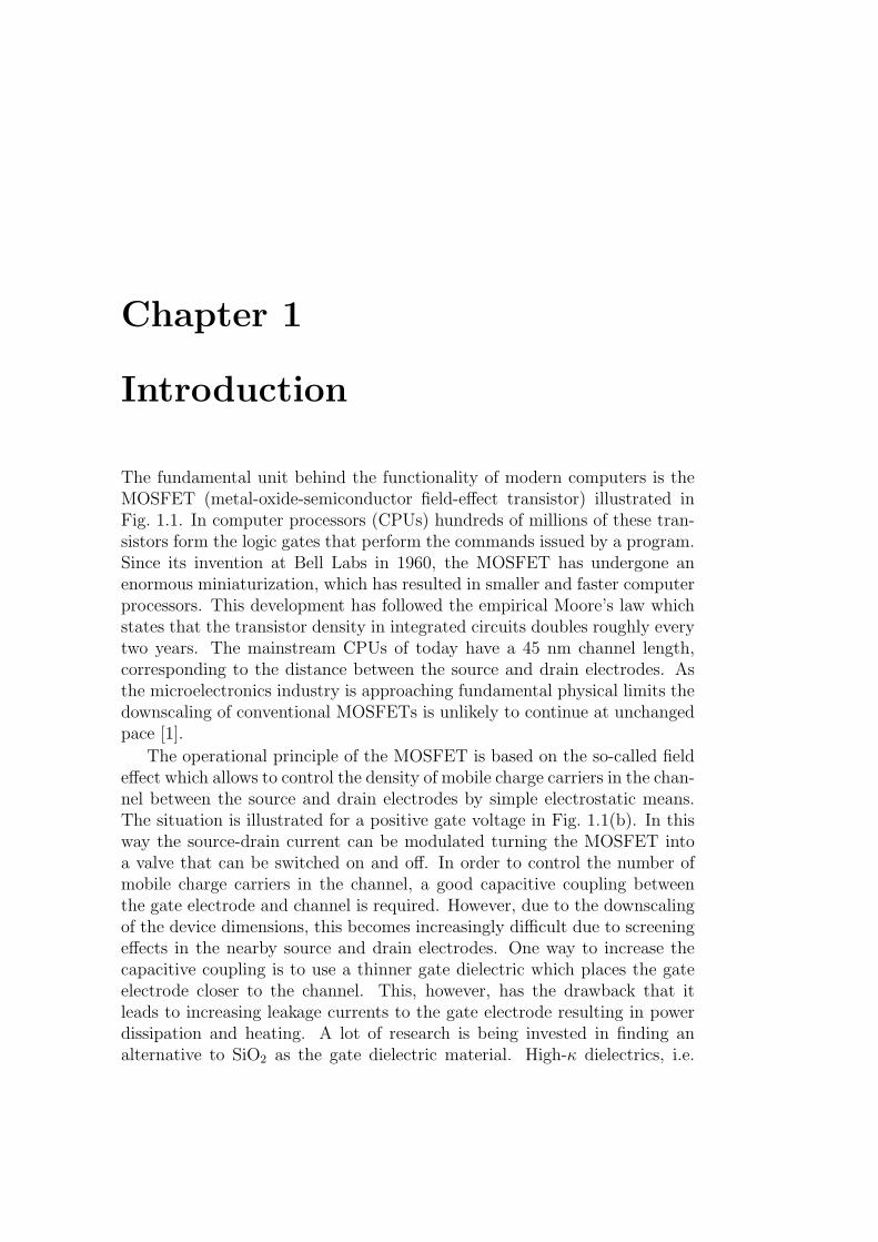
The fundamental unit behind the functionality of modern computers is theMOSFET (metal-oxide-semiconductor field-effect transistor) illustrated inFig. 1.1. In computer processors (CPUs) hundreds of millions of these tran-sistors form the logic gates that perform the commands issued by a program.Since its invention at Bell Labs in 1960, the MOSFET has undergone anenormous miniaturization, which has resulted in smaller and faster computerprocessors. This development has followed the empirical Moore’s law whichstates that the transistor density in integrated circuits doubles roughly everytwo years. The mainstream CPUs of today have a 45 nm channel length,corresponding to the distance between the source and drain electrodes. Asthe microelectronics industry is approaching fundamental physical limits thedownscaling of conventional MOSFETs is unlikely to continue at unchangedpace [1].
The operational principle of the MOSFET is based on the so-called fieldeffect which allows to control the density of mobile charge carriers in the chan-nel between the source and drain electrodes by simple electrostatic means.The situation is illustrated for a positive gate voltage in Fig. 1.1(b). In thisway the source-drain current can be modulated turning the MOSFET intoa valve that can be switched on and off. In order to control the number ofmobile charge carriers in the channel, a good capacitive coupling betweenthe gate electrode and channel is required. However, due to the downscalingof the device dimensions, this becomes increasingly difficult due to screeningeffects in the nearby source and drain electrodes. One way to increase thecapacitive coupling is to use a thinner gate dielectric which places the gateelectrode closer to the channel. This, however, has the drawback that itleads to increasing leakage currents to the gate electrode resulting in powerdissipation and heating. A lot of research is being invested in finding analternative to SiO2 as the gate dielectric material. High-κ dielectrics, i.e.

2 Introduction
(b)(a)
Figure 1.1: The MOSFET. (a) Cross sectional view of a MOSFET. The gateelectrode is separated from the transistor channel between the source and drainelectrodes by an insulating layer of dielectric material. (b) With a positive voltageapplied to the gate electrode a conducting channel is formed between the sourceand drain electrodes. Taken from Ref. [4].
oxides with a higher dielectric constant than SiO2 (εr = 3.9), allow for anincreased capacitive coupling to the channel without the need of decreasingthe thickness of the gate dielectric. However, the requirements for such areplacement are not few and research is still ongoing [2, 3].
While conventional silicon-based electronics has progressed, FETs basedon other materials have gained increasing interest. These include ex-amples such as organic FETs (OFETs) and organic thin film transistors(OTFT) in which an organic semiconductor is used as channel [5], self-assembled-monolayer FETs (SAMFETs) where a molecular monolayer con-stitute the channel [6], carbon nanotube FETs [7], and semiconductornanowire FETs [8]. Apart from conventional FET applications, these typesof transistors open up for interesting applications such as flexible displaysand various sensing devices [9].
1.1 Single-molecule electronics
The idea of using single molecules as the functional unit in electronic devicesoriginates from the theoretical work by Aviram and Ratner in 1974 [10].Their idea was that a rectifying behavior of a molecular device could be tai-lored into the molecule with functional donor and acceptor groups. However,only within the past two decades have experimental techniques that allow forsingle-molecule studies been developed. These include different microscopymethods such as scanning tunneling microscopy (STM) and atomic force
1.2 The single-electron transistor 3
microscopy (AFM) where the molecule is studied on a conducting substrate.More recently, the single-molecule version of the field effect transistor hasbeen realized [11]. Such three-terminal junctions have the advantage thatthey allow to tune the molecular levels independently of an applied bias.This is in contrast to e.g. STM measurements which lacks potential controlover the molecule. Here, the substrate and the tip function as source anddrain electrodes.
The progress within the field of single-molecule experiments has ledto many interesting observations. STM experiments probing a single or-ganic molecule on a silicon surface has shown negative differential resistance(NDR) [12]. A theoretical explanation ascribes this effect to a bias inducedshift of the current carrying molecular level which moves it inside the band-gap of the silicon substrate [13]. Other studies have demonstrated current-induced switching behavior due to molecular bistabilities [14, 15]. ImpressiveSTM and AFM measurements on single pentacene molecules have demon-strated that images of the molecular orbitals [16] and the molecular atomicstructure [17] can be obtained with very high resolution.
On the theoretical side a lot of work has been invested in understandingthe experimental observations. Furthermore, single-molecule devices exploit-ing the molecular electronic structure have been suggested. These includeexotic proposals as the quantum interference effect transistor (QuIET) [18]and the interference single-electron transistor (I-SET) [19]. The functionalityof these devices is based on interference effects that arises from the symmetryof the molecule combined with the coupling to the metallic electrodes.
With focus on factors that determine the electronic structure of single-molecule nanojunctions, the scope of the present work is more general. Partof this work is motivated by experimental observations on three-terminalsingle-molecule transistors [20]. Since their functionality is similar to that ofa single-electron transistor, a brief introduction to single-electron transistortheory is given in the following section. Subsequent sections present someintroductory considerations on single-molecule transistors and an overviewof relevant experimental results.
1.2 The single-electron transistor
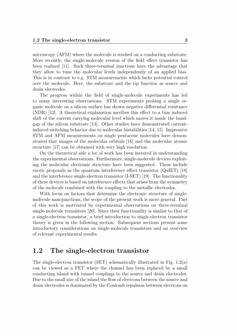
The single-electron transistor (SET) schematically illustrated in Fig. 1.2(a)can be viewed as a FET where the channel has been replaced by a smallconducting island with tunnel couplings to the source and drain electrodes.Due to the small size of the island the flow of electrons between the source anddrain electrodes is dominated by the Coulomb repulsion between electrons on

4 Introduction
Cs Cd
VdVs
Cg
Vg
(a) (b)
VI
Gate
Source Island Drain
Figure 1.2: Schematic illustration of a single-electron transistor. (a) The island isconnected to the source and drain electrodes with tunnel couplings. The energy ofthe island can be shifted with the gate electrode which couples capacitively to theisland. (b) Capacitor description of the single-electron transistor. The potentialof the island VI is determined by the voltages applied to the electrodes and thecharge Q on the island.
the island. For a given charge Q = −eN on the island, the Coulomb chargingenergy associated with the addition of another electron is considerable. Inorder to have a current flowing extra energy must therefore be provided bythe source-drain voltage. The resulting current is characterized by sequentialtunneling events, where single electrons one by one traverse the island. Thisclassical transport mechanism corresponds to the current to lowest order inthe tunnel couplings. Every time an electron tunnels to and off the island thenumber of electrons N on the island fluctuates by one. Due to the blockingof the current at low biases, this phenomenon is referred to as Coulombblockade.
Instead of increasing the source-drain voltage, the blockade can also belifted by applying a voltage Vg to the gate electrode. This results in a seriesof peaks in the differential conductance as a function of the gate voltageVg. This is illustrated in Fig. 1.3(a). The position of the peaks correspondsto gate voltages where a chemical potential µ of the island aligns with theFermi energy of the source and drain electrodes. The situation is sketchedin Fig. 1.3(b) for an arbitrary gate voltage. Consequently, at zero-bias con-ditions, only at these so-called charge degeneracy points will the island beable to change its charge and conduct a current between the source-drainelectrodes. In between the degeneracy points current is blocked and thenumber of electrons N on the island remains fixed. The distance betweenconsecutive peaks is termed the addition energy because it corresponds tothe energy needed to add another electron to the island.
A common approximation is to characterize the island with a capacitanceC. Within this approximation the Coulomb charging energy Ec becomes that

1.2 The single-electron transistor 5
Vg
sddI
/dV
N N+1N−1µN
Ef
µN+1
(a) (b)
ds
E
Figure 1.3: Differential conductance and level alignment of a single-electrontransistor. (a) Differential conductance dI/dVsd as a function of the gate voltageVg. Between the charge degeneracy points which are characterized by a peak in thedifferential conductance, the Coulomb blockade suppresses the current and leavesthe island with a constant number of electrons. (b) Alignment between the Fermienergies of the electrodes and the chemical potentials of the island. The chemicalpotentials of the island can be shifted with a gate voltage.
of a classical capacitor
Ec =e2
2C. (1.1)
This is the essence of the constant-interaction model which will be introducedin more detail in the following section. Depending on the nature of the islandquantum mechanical size quantization may become significant resulting ina level spacing ∆ between the island states. This leads to the followingexpression for the addition energy
Eadd = ∆ + 2Ec. (1.2)
Notice that only when ∆ small compared to Ec will the charge degeneracypeaks be equally spaced as illustrated in Fig. 1.3.
In order to be in the Coulomb blockade regime a necessary condition isthat the charging energy or the level spacing must be considerably higherthan the temperature,
Ec,∆ kBT,Γ. (1.3)
If this condition is not fulfilled thermal fluctuation will smear out the peakedstructure in the differential conductance with the result that N becomesundefined for all values of the gate voltage. Also the tunnel couplings to theelectrodes, which are here represented by a broadening Γ of the electroniclevels, must be small compared to the charging energy and level spacing.In the opposite limit, i.e. Γ Ec,∆, where quantum mechanical chargefluctuations dominate, the sequential tunneling picture no longer applies.

6 Introduction
In this regime the electrons travel phase-coherently between the source anddrain contacts. This is the situation in e.g. gate-defined quantum pointcontacts, where the conductance jumps in units of the conductance quantumG0 = e2/h every time a new electron channel in the contact enters the biaswindow.
SETs have so far been realized in a wide range of different nanostructures.This includes metal nanoparticles, gate defined quantum dots in semiconduc-tor structures, carbon nanotubes [21, 22], semiconducting nanowires [23, 24]and more recently single graphene sheets [25]. As the source-drain currentis highly sensitive to overall changes in the island potential, SETs can beoperated as ultra sensitive electrometers and have been used for e.g. real-time detection of individual electron tunneling events [26].
1.2.1 Constant-interaction model
The basic features in the IV-characteristics of different types of SETs can allbe understood from the constant-interaction model. This model is analogousto the capacitance model illustrated in Fig. 1.2(b) where the island is coupledcapacitively to the source, drain and gate electrodes with capacitances Cs,Cd and Cg. The potential VI of the island is left floating. The integer chargeon the island is represented by the sum of the charges Qi on the individualcapacitor electrodes, i.e. −eN =
∑iQi. Each of the charges Qi follows from
the usual relation between charge and voltage on a capacitor, Qi = Ci(Vi−VI),where Vi denotes the voltage applied to the i’th electrode. With N electronson the island the energy of the system is given by the sum of the electrostaticenergy and the single-particle energies [27]
E(N) =[e(N −N0)− CgVg]
2
2C+
N∑n=1
εn, (1.4)
where N0 is the number of electrons on the neutral island at Vg = 0, C =Cs+Cd+Cg is the total capacitance and εn are the discrete energy levels of theisland arising due to size quantization. The term CgVg is a continuous variablethat represents the gate induced charge on the island. The name constant-interaction model stems from the fact that the capacitances which accountfor the Coulomb repulsion on the island are considered to be independent ofthe applied voltages and the number of electrons N on the island. This isonly a good approximation when the quantum states in which electrons areinserted have similar spatial distributions on the island and do not changewith the applied voltages. As the present work will demonstrate, this isquestionable when the island is a single molecule.

1.2 The single-electron transistor 7
Vsd
Vg
add /eE
Eadd /αe
2α
NN−1 N+1
Figure 1.4: Charge stability diagram for a single-electron transistor showingschematically the current as a function of bias and gate voltage. Inside the blackdiamonds the current is blocked. The diamond edges corresponds to a situationwhere a chemical potential of the island passes through the Fermi energy of one ofthe electrodes. As indicated, values for the addition energy Eadd and gate couplingα can be extracted from the diamonds.
At the charge degeneracy points discussed in the previous section thechemical potential of the island µN = E(N)− E(N − 1) is aligned with theFermi energies of the source and drain electrodes. With the energy given byEq. (1.4) the chemical potential of the island can be written
µN = (2N − 1)Ec − eαVg + εN (1.5)
The change of the chemical potential with an applied gate voltage carriesa prefactor α = Cg/C. This is the gate coupling which depends on thegeometry of the sample. Due to the screening from the source and drainelectrodes the gate coupling will always be less than unity, i.e. α < 1. Asthe addition energy corresponds to the difference between adjacent chemicalpotentials,
Eadd = µN+1 − µN , (1.6)
the expression in Eq. (1.2) readily follows with ∆ = εN+1−εN . It is importantto note that the distance between the charge degeneracy peaks on the gatevoltage axis in Fig. 1.3 does not correspond to the actual addition energy.Due to the screening of the gate potential it is instead given by the additionenergy scaled with the inverse of the gate coupling, Eadd/(eα).
As a function of both gate and source-drain voltage the regions in whichthe current is blocked forms a diamond-shaped structure as illustrated inFig. 1.4. These so-called diamond plots, or charge stability diagrams, are veryuseful when studying the properties of a given device. As indicated in thefigure, quantitative information about the gate coupling and addition energy

8 Introduction
GaAs 10 nm 500 nm single
quantum dot metallic island carbon nanotube molecule
∆ ∼ 0.1 meV 1 meV 3 meV > 0.1 eV
Ec ∼ 1 meV 25 meV 3 meV > 0.1 eV
Table 1.1: Typical level spacing and charging energies for different types ofsingle-electron transistors [28].
can be inferred from these plots. When the bias is applied symmetrically tothe source and drain electrodes, the slopes of the diamond edges are givenby ±2α. The addition energy can be obtained both from the width and theheight of the diamonds. For the latter, this relies on the assumption thatthe applied source-drain voltage does not change the energy of the island –i.e. only the Fermi energies of the electrodes are shifted by the applied bias.In order for this to hold, the source and drain electrodes must have equalcapacitive couplings to the island.
1.3 Single-molecule SETs
During the past decade there has been a significant progress in the experimen-tal techniques for the fabrication of three-terminal single-molecule devices.This has allowed for the realization of the molecular version of the single-electron transistor. A major difference between single-molecule SETs andconventional SETs based on gate defined quantum dots in semiconductorsstructures and metallic nanoparticles is the size of the level spacing andcharging energy. In Tab. 1.1 typical level spacing and charging energies forvarious SETs are summarized. Due to the relative small sizes of moleculesboth their levels spacings and charging energies of single-molecule SETS areconsiderably higher than those of other SET types. This, in principle, allowsfor room temperature operation since Ec,∆ > kBT ∼ 26 meV. At present,however, the stability of single-molecule SETs at non-cryogenic temperaturesis still an open issue [4].
In the following sections a brief overview of fabrication techniques andexperimental results for single-molecule SETs will be given. Moreover, someconsideration relevant for the present work are presented. Further insight intothe field is provided by the numerous review papers which have appeared overthe recent years [4, 28, 29, 30, 31, 32].
1.3 Single-molecule SETs 9
1.3.1 Fabrication techniques
The experimental realization of a single-molecule SET relies on the fabrica-tion of a three-terminal junction with a molecule bridging a nanoscale gapbetween the source and drain electrodes and a gate electrode placed closeenough to the gap that it couples capacitively to the molecule. In Fig. 1.5various techniques for this purpose are illustrated schematically. They mainlydiffer in the way the electrodes and the nanogap between them are created.In single-molecule SETs it is important that the gap is neither too long forthe molecule to connect to both electrodes, or too small in which case a goodgate coupling to the molecule becomes difficult to obtain. The three standardmethods are (i) electromigration, (ii) angle evaporation, and (iii) mechanicalbreak junction techniques.
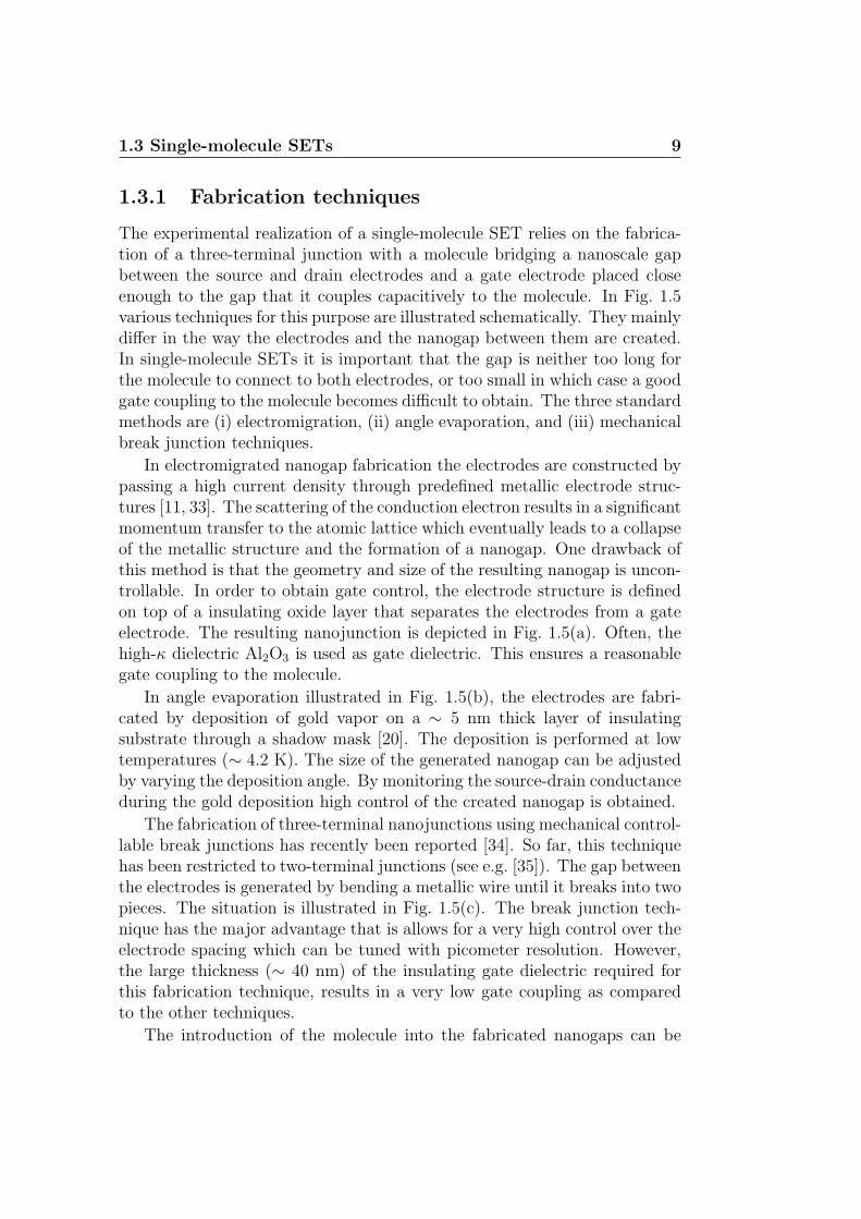
In electromigrated nanogap fabrication the electrodes are constructed bypassing a high current density through predefined metallic electrode struc-tures [11, 33]. The scattering of the conduction electron results in a significantmomentum transfer to the atomic lattice which eventually leads to a collapseof the metallic structure and the formation of a nanogap. One drawback ofthis method is that the geometry and size of the resulting nanogap is uncon-trollable. In order to obtain gate control, the electrode structure is definedon top of a insulating oxide layer that separates the electrodes from a gateelectrode. The resulting nanojunction is depicted in Fig. 1.5(a). Often, thehigh-κ dielectric Al2O3 is used as gate dielectric. This ensures a reasonablegate coupling to the molecule.
In angle evaporation illustrated in Fig. 1.5(b), the electrodes are fabri-cated by deposition of gold vapor on a ∼ 5 nm thick layer of insulatingsubstrate through a shadow mask [20]. The deposition is performed at lowtemperatures (∼ 4.2 K). The size of the generated nanogap can be adjustedby varying the deposition angle. By monitoring the source-drain conductanceduring the gold deposition high control of the created nanogap is obtained.
The fabrication of three-terminal nanojunctions using mechanical control-lable break junctions has recently been reported [34]. So far, this techniquehas been restricted to two-terminal junctions (see e.g. [35]). The gap betweenthe electrodes is generated by bending a metallic wire until it breaks into twopieces. The situation is illustrated in Fig. 1.5(c). The break junction tech-nique has the major advantage that is allows for a very high control over theelectrode spacing which can be tuned with picometer resolution. However,the large thickness (∼ 40 nm) of the insulating gate dielectric required forthis fabrication technique, results in a very low gate coupling as comparedto the other techniques.
The introduction of the molecule into the fabricated nanogaps can be

10 Introduction
Figure 1.5: Illustration of different single-molecule junction fabrication tech-niques. (a) Electromigrated thin metal wire on top of a Al/Al2O3 gate electrode.(b) Angle evaporation technique to fabricate planar electrodes with nanometerseparation on top of a Al/Al2O3 gate electrode. (c) Gated mechanical break junc-tion. (d) The dimer contacting scheme in which the molecule is attached to goldparticles. Figure taken from Ref. [31].
accomplished in different ways. One option is to subject the junction toa solution containing the molecule either prior to gap formation or after-ward and then hope that a molecule will be caught in the gap between theelectrodes. Alternatively, the molecules can be deposited on the electrodesby quench condensation [20]. By subsequent annealing the sample at lowtemperature (below 70 K), the molecules are allowed to diffuse. The pres-ence of a molecule in the nanogap is detected by monitoring the source-drainconductance. When it changes markedly, the sample is cooled to cryogenictemperatures and IV-characteristics on the single molecule can be carriedout.
In order to control the chemical coupling between the source and drainelectrodes, the molecules are often prepared with chemical groups that eitherfacilitates or prevents bonding to the metallic electrodes. It has recentlybeen demonstrated that this approach allows to obtain a high control of theelectrode-molecule coupling [36] which is essential for the device characteris-tics. With a large metal-molecule coupling Γ the Coulomb blockade require-ments in Eq. (1.3) are not necessarily fulfilled. Indeed, it was demonstrated
1.3 Single-molecule SETs 11
that in this strong coupling regime the conductance showed no significantdependence on the gate voltage, and consequently, no Coulomb blockadecharacteristics were observed. On the other hand, when molecules are pre-pared with for example passivated thiol groups [20] or no chemical groups atall, only the weak van der Waals force binds the molecule to the electrodes.As a result, the device acquires SET functionality. This is the observedbehavior of the majority of single-molecule junctions fabricated as describedin the present section.
Another approach for controlling the electrode-molecule coupling is thedimer contacting scheme illustrated in Fig. 1.5(d) [37]. Here, the molecule isprepared with two gold particles which are connected to the molecule withthiol bonds. The gold particles allows to trap the dimer structure betweenthe electrodes electrostatically. This approach has the inherent disadvantagethat the gate coupling is low due to efficient screening in the gold particles.
From the present section it is clear that the techniques for fabricationof single-molecule SETs are highly statistical in nature. Therefore, no twodevices will show exactly the same results and technological applicationsof single-molecule transistors should not be expected within the foreseeablefuture. Nevertheless, single-molecule SETs give the opportunity to studyexciting physics and chemistry at the single-molecule level. Compared tosingle-molecule experiments using electrochemical gating at room tempera-ture [38, 39, 40], the cryogenic solid-state environment of a single-moleculeSET seems to be better suited for studying the fundamental role of the molec-ular degrees of freedoms on the charge transport through the molecule. Forexample, recent developments doing simultaneous conduction measurementsand Raman spectroscopy on a single-molecule junction provides detailed in-formation about the vibrational modes that play an active role in the electrontransport [41, 42].
1.3.2 Addition energy
In single-molecule SETs the chemical potentials associated with the removaland addition of an electron from the neutral molecule are given by the molec-ular ionization potential (IP) and electron affinity (EA). They are defined bythe total energy difference between the two charge states involved in the elec-tron transfer, i.e. IP = EN−1−EN and EA = EN −EN+1, where N denotesthe number of electrons in the neutral molecule. The difference between theIP and EA defines the fundamental gap Egap of a molecule
Egap = IP− EA = EN+1 + EN−1 − 2EN . (1.7)

12 Introduction
~
εr
Dielectric
ds
Gate
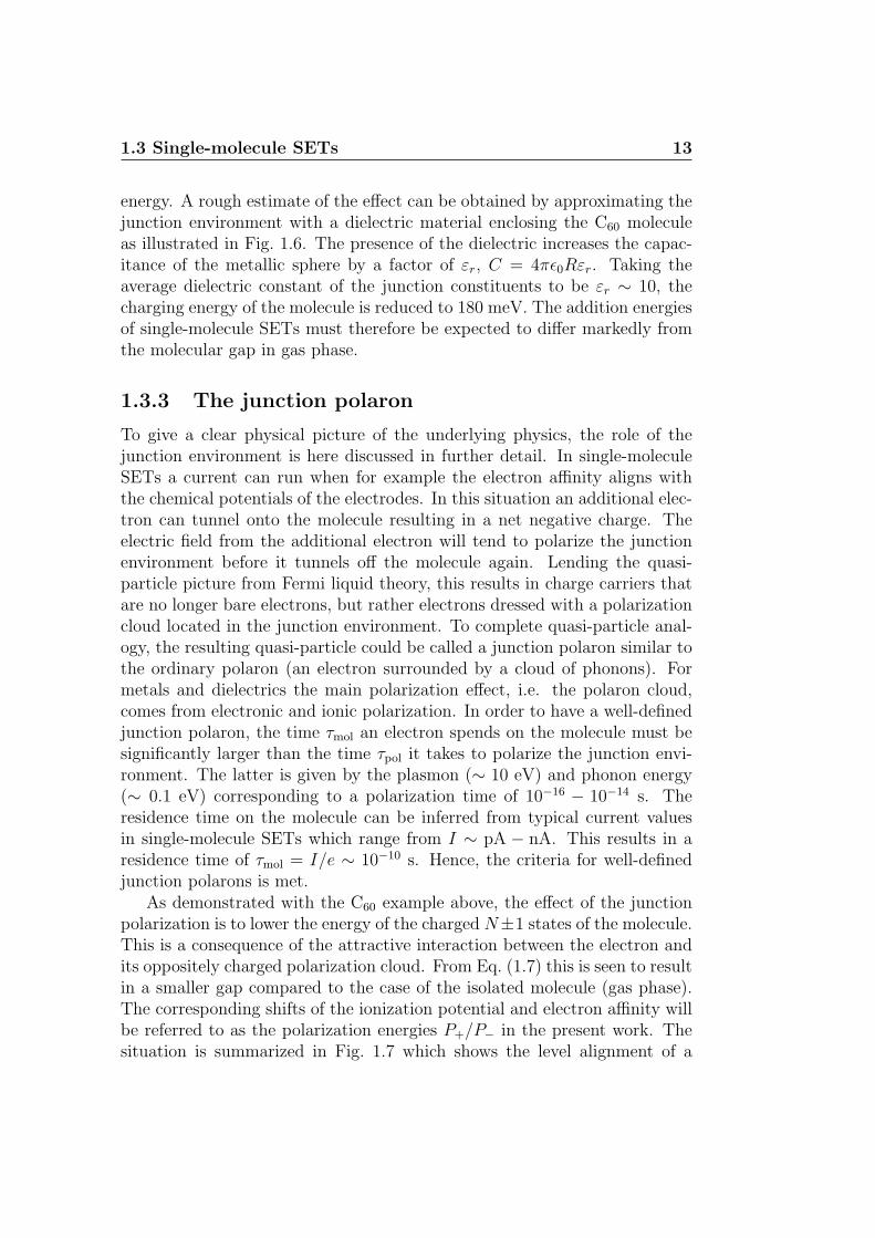
Figure 1.6: Schematic illustration of a nanojunction with a C60 molecule placedbetween the source and drain electrodes. In a simple approximation the effect ofthe junction environment can be described by a dielectric material with εr ∼ 10enclosing the molecule. In a capacitor description of the C60 molecule (see text)the capacitance is given by C = 4πε0Rεr. Hence, the charging energy Ec = e2/2cof the molecule is strongly reduced in the junction.
In the SET framework the molecular gap corresponds to the addition energyin Eq. (1.6) of the neutral molecule. In a simplified single-particle descriptionof the electronic structure of the molecule, the addition energy of a single-molecule SET takes a form equivalent to that of the constant interactionmodel in Eq. (1.2). The level spacing ∆ is replaced by the HOMO-LUMOgap ∆HL of the molecule, where HOMO and LUMO refers to the highest occu-pied and lowest unoccupied molecular orbital, respectively, and the chargingenergy Ec is the Coulomb energy it costs to remove (add) an electron to theHOMO (LUMO). Typical values for ∆HL and Ec for isolated molecules areon the order of several electron-volts.
The following example consider the addition energy of the C60 molecule interms of a simple capacitor model for the charging energy. The C60 moleculehas an ionization potential and electron affinity of IP = 7.6 eV and EA =2.65 eV [43], respectively. This results in a gap of Egap = 4.95. In a simplifieddescription of the C60 molecule the charging energy can be approximated bythat of a metal sphere with capacitance
C = 4πε0R, (1.8)
where ε0 is the vacuum permittivity and R is the radius of the sphere. Set-ting R = 4 A, corresponding to the radius of the C60 molecule, the chargingenergy in Eq. (1.1) amounts to Ec ∼ 1.8 eV, leaving 1.35 eV for the HOMO-LUMO gap. It should be noted that these consideration are only valid forthe isolated molecule. When placed in a three-terminal nanojunction as illus-trated in Fig. 1.6, the molecule is surrounded by metallic electrodes and gatedielectric which increases the capacitance and leads to a smaller charging
1.3 Single-molecule SETs 13
energy. A rough estimate of the effect can be obtained by approximating thejunction environment with a dielectric material enclosing the C60 moleculeas illustrated in Fig. 1.6. The presence of the dielectric increases the capac-itance of the metallic sphere by a factor of εr, C = 4πε0Rεr. Taking theaverage dielectric constant of the junction constituents to be εr ∼ 10, thecharging energy of the molecule is reduced to 180 meV. The addition energiesof single-molecule SETs must therefore be expected to differ markedly fromthe molecular gap in gas phase.
1.3.3 The junction polaron
To give a clear physical picture of the underlying physics, the role of thejunction environment is here discussed in further detail. In single-moleculeSETs a current can run when for example the electron affinity aligns withthe chemical potentials of the electrodes. In this situation an additional elec-tron can tunnel onto the molecule resulting in a net negative charge. Theelectric field from the additional electron will tend to polarize the junctionenvironment before it tunnels off the molecule again. Lending the quasi-particle picture from Fermi liquid theory, this results in charge carriers thatare no longer bare electrons, but rather electrons dressed with a polarizationcloud located in the junction environment. To complete quasi-particle anal-ogy, the resulting quasi-particle could be called a junction polaron similar tothe ordinary polaron (an electron surrounded by a cloud of phonons). Formetals and dielectrics the main polarization effect, i.e. the polaron cloud,comes from electronic and ionic polarization. In order to have a well-definedjunction polaron, the time τmol an electron spends on the molecule must besignificantly larger than the time τpol it takes to polarize the junction envi-ronment. The latter is given by the plasmon (∼ 10 eV) and phonon energy(∼ 0.1 eV) corresponding to a polarization time of 10−16 − 10−14 s. Theresidence time on the molecule can be inferred from typical current valuesin single-molecule SETs which range from I ∼ pA − nA. This results in aresidence time of τmol = I/e ∼ 10−10 s. Hence, the criteria for well-definedjunction polarons is met.
As demonstrated with the C60 example above, the effect of the junctionpolarization is to lower the energy of the charged N±1 states of the molecule.This is a consequence of the attractive interaction between the electron andits oppositely charged polarization cloud. From Eq. (1.7) this is seen to resultin a smaller gap compared to the case of the isolated molecule (gas phase).The corresponding shifts of the ionization potential and electron affinity willbe referred to as the polarization energies P+/P− in the present work. Thesituation is summarized in Fig. 1.7 which shows the level alignment of a

14 Introduction
E fP+
P−
W
E
EA
V g
IP
vacuum
Figure 1.7: Energy level alignment in a single-molecule transistor. The polariza-tion of the junction renormalizes the molecular ionization energy (IP) and electronaffinity (EA) by the polarization energies P+/−, respectively. The alignment be-tween the Fermi energy of the source and drain electrodes and the molecular levelsdetermine the threshold for electron transport through the junction.
single-molecule SET.
As the threshold for electron transport through the molecule is deter-mined by the alignment between the molecular levels and the Fermi energyof the electrodes, the properties of single-molecule SETs are highly depen-dent on the size of the polarization energies. In order to obtain quantitativeestimates for the polarization energies in single-molecule SETs, a quantummechanical calculation of the total energies in Eq. (1.7) including the effectof junction polarization is required. A theoretical framework for this purposeis presented in Chap. 2.
Other polarizable environments
The effect of environmental polarization on molecular levels is well knownfrom other fields. In electrochemistry charging processes of single moleculestake place under potential control in ionic solutions at room temperature.Here, the analog of the polarization energies P± is the solvation free energywhich describes the effect of solvent polarization [44]. The measured redoxpotentials of a given molecule are equivalent to the charge degeneracy pointsof a single-molecule SET. However, due to the different environmental situa-tion, direct comparison between the two are not possible. For example, bothresponse time and screening length are expected to differ markedly for thepolarization of a ionic solvent and solid state environment. Fig. 1.8 illustratesthe various contributions to the dielectric response and their characteristicfrequencies. While solvent screening is characterized by orientational polar-

1.3 Single-molecule SETs 15
Figure 1.8: Characteristic frequencies of various polarization mechanisms show-ing their contribution to a generic dielectric function εr = ε′r + iε′′r . Taken fromRef. [2].
ization with relatively low frequencies, the electronic and ionic solid statescreening have significantly higher frequencies. This implies that screeningof dynamical electron transfer processes will in general be more efficient insolid state environments.
Polarization is also an important factor for electron transport in organicsemiconductor crystals. Due to the weak van der Waals bonds between themolecular units the electronic structure of organic semiconductors is charac-terized by narrow bands (∼ 0.1 eV). This renders a band description withdelocalized Bloch states inappropriate. As a consequence, charge transportin these materials is better characterized by incoherent hopping betweenlocalized states on the molecular units. Due to the relatively long residencetime on the individual molecular units (given by the bandwidth), the polaronpicture also applies here. In this case, however, the polaron cloud is formed byelectronic polarization of the neighboring molecular units. The polarizationenergies in organic semiconductors are on the order of P± ∼ 1 − 2 eV [45],leaving the band gap of the crystal significantly smaller than the gap of theisolated molecule.
1.3.4 Experimental overview
Due to the weak coupling between the electrodes and the molecule, single-molecule SETs allows to study electron transport through well-defined statesof the molecule. For excited states this gives rise to additional featuresin the charge stability diagram apart from the Coulomb diamonds. Fromthese features the nature and the energy of the excitations can be inferred.
16 Introduction
Single-molecule SETs therefore provides a means of doing single-moleculespectroscopy in solid-state environments.
Over the past decade this has led to interesting observations of both thetransport mechanism and molecular properties in single-molecule SETs. Forexample, in a pioneering work on the C60 molecule, it has been demonstratedthat the tunneling of electrons can excite vibrational modes associated withthe center-of-mass motion of the molecule [11]. In the charge stability di-agram such excitations shows up as lines parallel to the diamond edges.In experiments on single-molecule magnets the magnetic properties of themolecules has been addressed [46, 47, 48]. From the charge stability diagramthe different spin excitations of the molecule could be identified showingthat the molecules remain magnetic in the solid-state junction environment.Moreover, the molecular spin degree of freedom was found to play an impor-tant role for the transport through the molecule.
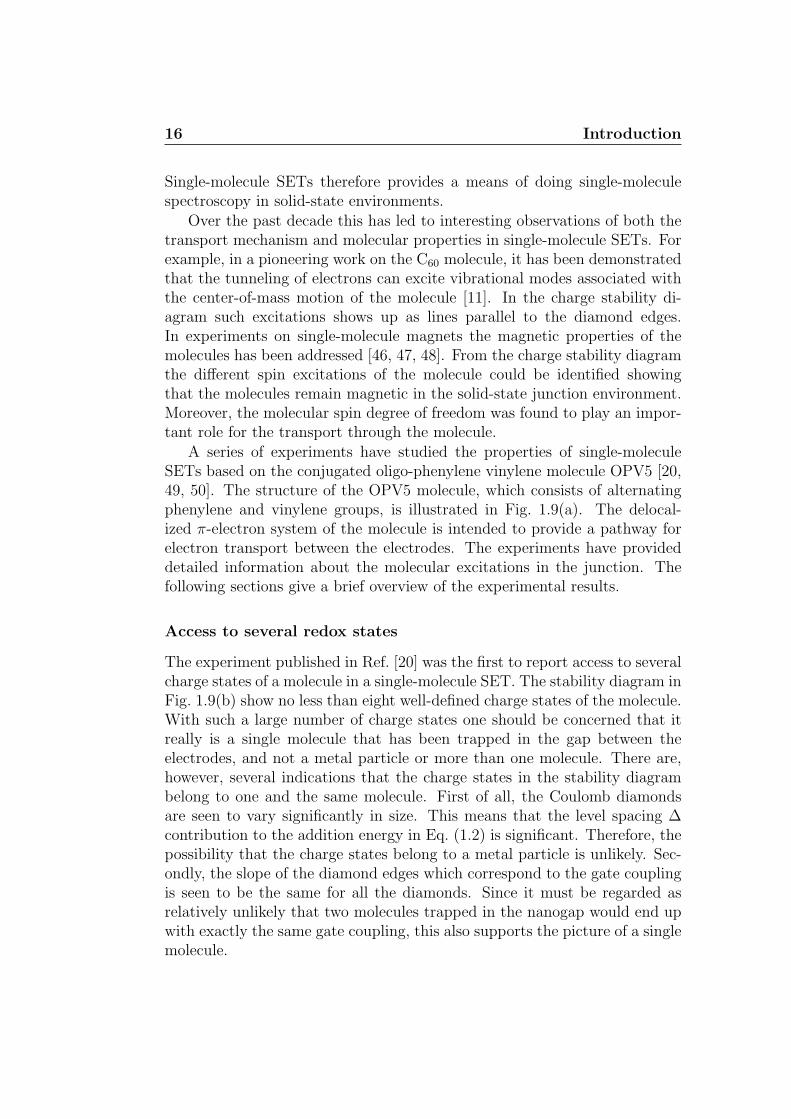
A series of experiments have studied the properties of single-moleculeSETs based on the conjugated oligo-phenylene vinylene molecule OPV5 [20,49, 50]. The structure of the OPV5 molecule, which consists of alternatingphenylene and vinylene groups, is illustrated in Fig. 1.9(a). The delocal-ized π-electron system of the molecule is intended to provide a pathway forelectron transport between the electrodes. The experiments have provideddetailed information about the molecular excitations in the junction. Thefollowing sections give a brief overview of the experimental results.
Access to several redox states
The experiment published in Ref. [20] was the first to report access to severalcharge states of a molecule in a single-molecule SET. The stability diagram inFig. 1.9(b) show no less than eight well-defined charge states of the molecule.With such a large number of charge states one should be concerned that itreally is a single molecule that has been trapped in the gap between theelectrodes, and not a metal particle or more than one molecule. There are,however, several indications that the charge states in the stability diagrambelong to one and the same molecule. First of all, the Coulomb diamondsare seen to vary significantly in size. This means that the level spacing ∆contribution to the addition energy in Eq. (1.2) is significant. Therefore, thepossibility that the charge states belong to a metal particle is unlikely. Sec-ondly, the slope of the diamond edges which correspond to the gate couplingis seen to be the same for all the diamonds. Since it must be regarded asrelatively unlikely that two molecules trapped in the nanogap would end upwith exactly the same gate coupling, this also supports the picture of a singlemolecule.

1.3 Single-molecule SETs 17
(b)
(a)
Figure 1.9: Molecular structure and stability diagram showing access to sev-eral charge states of the OPV5 molecule [20]. (a) Molecular structure of a thiol-terminated OPV5 molecule. (b) Charge stability diagram showing access to severalcharge (redox) states of OPV5. The polarization of the junction environment mostlikely plays an important role for the stability of the large number of observedcharge states (see text).
From the complete diamonds corresponding to the charge states Q ± 1of the molecule, a gate coupling of ∼ 0.2 can be inferred. As the widthof the diamonds are given by Eadd/(eα), the addition energy of the neutralmolecule which corresponds to the gap of the molecule in the junction, canbe estimated to ∼ 200 − 300 meV. As discussed in Secs. 1.3.2 and 1.3.3,molecular gaps are expected to be reduced significantly in polarizable junc-tion environments. This is also the interpretation of Ref. [20], which ascribesthe origin of the small gap to image charges, i.e. polarization, in the metalelectrodes. For reference, the electrochemical gap of the OPV5 molecule wasreported to be ∼ 2.5 eV. Independent density functional calculation usingthe B3LYP exchange-correlation functional yields a gap of ∼ 4.5 eV for theisolated molecule. Based on the considerations from the simple capacitormodel of the C60 molecule in Sec. 1.3.2, the reduction of the sum of theHOMO-LUMO gap and the charging energy to a few hundreds of electron-volts seems drastic.
The large difference between the gap of the molecule in the SET envi-

18 Introduction
ronment and the electrochemical gap has fueled a discussion whether theinterpretation of this experiment is correct [4, 29]. In electrochemical mea-surements the compensating ions that stabilize the non-neutral redox statesof the molecule are only a few A distant from the molecule. Accordingly, thescreening should be more efficient than in a nanojunction. However, the smallgap observed in the single-molecule SET suggests the opposite. As pointedout in Sec. 1.3.3, the screening properties of a ionic solution at room tempera-ture and a solid-state environment cooled to cryogenic temperatures are verydifferent. This makes a direct comparison between them difficult. Anotherargument against the single molecule interpretation of the stability diagramin Fig. 1.9(b), is the large number of observed charge states which must posea serious challenge for the chemical stability of the molecule. However, theefficient screening of the junction environment play a stabilizing role for thecharge states of the molecule. This could be a decisive factor for the chemicalstability of the molecule in the large number of charged states observed.
It should be noted that the stability diagram in Fig. 1.9(b) is the onlyobservation of such a large number of charge states in a single-molecule SETso far. This, in conjunction with the fact that weakly coupled molecules insolid-state environments held at cryogenic temperatures is still a relativelyunexplored field, must leave the correct interpretation of this experiment asan open question. There is, however, no question that polarization playsan important role for the position of the molecular levels in single-moleculeSETs. In experiments where full Coulomb diamonds have been measured,small addition energies have been observed consistently. In Chap. 4 a quan-titative estimate of the effect in a realistic OPV5 single-molecule SET ispresented.
Spin excitations and Kondo effect
The stability diagram from another experiment on the OPV5 molecule isshown in Fig. 1.10(a) [49]. The schematic drawing in Fig. 1.10 gives anoverview of the important information in the stability diagram and the chargestates of the diamonds. Similar to the stability diagram in Fig. 1.10, the di-agram here consists of diamonds with varying size. As discussed in the pre-vious section this is an indication of the molecule being the active transportpathway for electron tunneling between the electrodes. Another similarity isthe small addition energies associated with the charged states. The additionenergy for the Q = +1 state is ∼ 50 meV which is in good agreement with thevalue for the same charge state in Fig. 1.10(a). Thus, also in this experimentdoes junction screening seem to be pronounced.
The horizontal features inside the Coulomb diamonds originate from

1.3 Single-molecule SETs 19
(b)(a)
Figure 1.10: Kondo effect and singlet-triplet excitation [49]. (a) Charge stabil-ity diagram for the OPV5 molecule showing features from higher-order tunnelingprocesses inside the Coulomb diamonds. (b) Schematic drawing showing the im-portant information contained in the stability diagram. The Kondo effect showsup as a zero-bias feature inside the Q = +1,+3 diamonds. The two parallellines inside the Q = +2 diamond are due to inelastic cotunneling that leaves themolecule in the excited triplet state (see text).
higher-order tunneling processes. An example is the Kondo effect whichmanifests itself in a zero-bias resonance inside the Coulomb diamonds in thestability diagram [51, 52]. In Fig. 1.10 this gives rise to the horizontal lines atzero bias inside the Q = +1,+3 diamonds. The Kondo resonance arises froma correlated many-body state between a single electron spin on the moleculeand the conduction electrons of the leads. Since it requires an unpairedelectron spin on the molecule, the zero-bias Kondo resonance appears onlyin diamonds with odd number of electrons. Hence, the presence of a Kondoresonance can be used to identify the charge states of the measured diamonds.
The two parallel lines inside the Q = +2 diamond come from inelasticcotunneling processes which are next-to-leading order in the tunnel couplingbetween the molecule and the leads. Cotunneling describes processes in whichan electron is transferred between the electrodes via an intermediate state ofthe molecule that can have a higher energy than the initial state. In inelasticcotunneling the molecule is left in an excited state which is why it shows up atfinite bias values. In the present case a splitting of the inelastic cotunnelinglines in a magnetic field allowed to connect them with the excited tripletstate of the doubly charged OPV5 molecule. The energy splitting betweenthe singlet ground state and the excited triplet state can be inferred fromthe distance between the zero-bias axis and the cotunneling lines. It hereamounts to ∼ 1.7 meV. The singlet-triplet splitting can be accounted for
20 Introduction
by an effective antiferromagnetic exchange coupling J between two spatiallyseparated single-particle states A and B holding the unpaired electrons ofthe doubly charged molecule,
H = JSA · SB, (1.9)
where SA/B denotes the spin operators. The spatially separated states Aand B were ascribed to image charge stabilized localizations of the unpairedspins at the terminating phenylene units in each end of the molecule. Thisserves to illustrate that the junction polarization not only affects the size ofthe Coulomb diamonds but also the excitation spectrum of the molecule.
Vibrational excitations
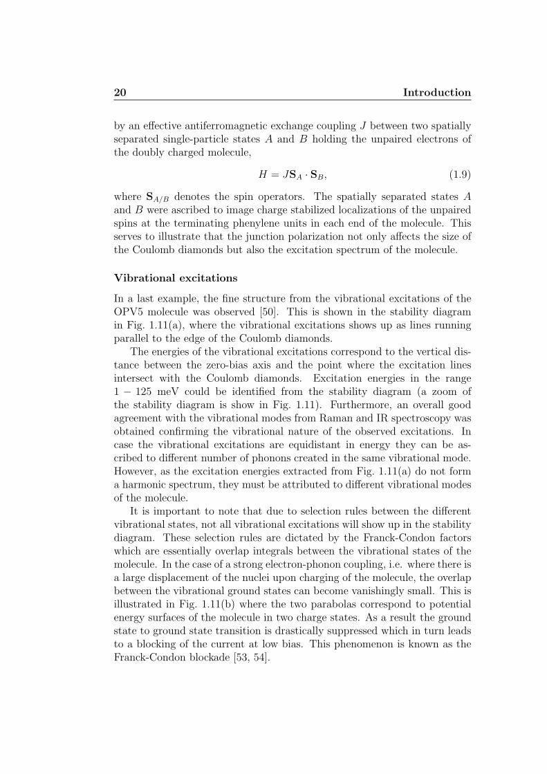
In a last example, the fine structure from the vibrational excitations of theOPV5 molecule was observed [50]. This is shown in the stability diagramin Fig. 1.11(a), where the vibrational excitations shows up as lines runningparallel to the edge of the Coulomb diamonds.
The energies of the vibrational excitations correspond to the vertical dis-tance between the zero-bias axis and the point where the excitation linesintersect with the Coulomb diamonds. Excitation energies in the range1 − 125 meV could be identified from the stability diagram (a zoom ofthe stability diagram is show in Fig. 1.11). Furthermore, an overall goodagreement with the vibrational modes from Raman and IR spectroscopy wasobtained confirming the vibrational nature of the observed excitations. Incase the vibrational excitations are equidistant in energy they can be as-cribed to different number of phonons created in the same vibrational mode.However, as the excitation energies extracted from Fig. 1.11(a) do not forma harmonic spectrum, they must be attributed to different vibrational modesof the molecule.
It is important to note that due to selection rules between the differentvibrational states, not all vibrational excitations will show up in the stabilitydiagram. These selection rules are dictated by the Franck-Condon factorswhich are essentially overlap integrals between the vibrational states of themolecule. In the case of a strong electron-phonon coupling, i.e. where there isa large displacement of the nuclei upon charging of the molecule, the overlapbetween the vibrational ground states can become vanishingly small. This isillustrated in Fig. 1.11(b) where the two parabolas correspond to potentialenergy surfaces of the molecule in two charge states. As a result the groundstate to ground state transition is drastically suppressed which in turn leadsto a blocking of the current at low bias. This phenomenon is known as theFranck-Condon blockade [53, 54].
1.3 Single-molecule SETs 21
(a) (b)
Figure 1.11: Vibrational excitations of the OPV5 molecule [50]. (a) Stabilitydiagram with a detailed fine structure from the vibrational excitations of the OPV5molecule. The excitations appears as lines parallel to the diamonds edges. (b)Potential energy surfaces as a function of a general nuclei coordinate q for twocharge states of a molecule. For a strong electron-phonon coupling the horizontaldisplacement between the energy surfaces is large resulting in a suppression of thetransition indicated by the green arrow. This gives rise to the Franck-Condonblockade (see text).
1.3.5 Theoretical descriptions
Theoretical descriptions of single-molecule SETs are typically based on atwo-step procedure. In the first step the molecular states which are involvedin the electron transport are determined. In a second step, the current iscalculated from a stationary solution to the so-called Master equations. Thefollowing section gives a brief overview of this approach together with someconsiderations on different methods for the determination of the molecularstates.
The starting point is the following generic junction Hamiltonian
H = Hmol +Hleads +Ht (1.10)
where Hmol denotes the Hamiltonian of the molecule, Hleads the Hamiltonianof the electrodes and Ht the tunnel coupling between the two. Due to theweak tunnel coupling the states of the molecule are assumed to be unaffectedby the tunnel coupling. Hence, they can be obtained as the many-body statesof Hmol which are characterized by the number of electrons N on the moleculeand a general index i referring to some excited state of the molecule. Underfinite bias conditions the occupations of the |N, i〉-states are given by a non-equilibrium probability distribution PN,i for the states. Treating Ht as aperturbation, the transition rates Γ between the molecular states can bedescribed using Fermi’s Golden rule.

22 Introduction
Knowing the transition rates, the probability for being in the i’th excitedN -electron can be found from the equation
d
dtPN,i =
∑j
[−(ΓN+1,j
N,i+ ΓN−1,j
N,i
)PN,i + Γ N,i
N+1,jPN+1,j + Γ N,i
N−1,jPN−1,j
],
(1.11)which gives the time-derivative of the probability in terms of the rates fortunneling in and out of the state. The set of equation formed by the prob-abilities for all the considered states are usually referred to as the masterequations. From a stationary solution for the probabilities, i.e. d/dtPN,i = 0,the current from the sequential tunnel processes can be obtained [55].
The molecular states |N, i〉 enter the transition rates. The rates for in-creasing the number of electrons by one are given
ΓN+1,jN,i
=2π
~∑
α
Γαj,ifα(Eij), (1.12)
where fα is the fermi distribution of the electrodes, Eij = EN+1j − EN
i isthe total energy difference between the molecular states. In the case of iand j referring to ground states of the N and N + 1 electron molecules,Eij corresponds to the electron affinity (see (1.7)). The alignment betweenthe Fermi energy of the electrodes and the molecular levels are thereforecontained in the Fermi function. The factor Γα
j,i is given by
Γαj,i = ρα |tα|2
∣∣〈N + 1, j|c†|N, i〉∣∣2 . (1.13)
Here, tα denotes the tunnel matrix element to the electrodes and ρα is thedensity of states of the electrodes. It is the matrix element between thestates |N, i〉 and |N+1, j〉 that determines the selection rules for the current-induced transitions between two molecular states. For vibrational excitationsthe Franck-Condon factors constitute the part of the overlap that deals withthe vibrational degrees of freedom.
Since the master equation approach is based on a perturbative treatmentto lowest order in the tunneling Hamiltonian Ht, the width of the resonancesis determined solely by the temperature. Therefore,
Ec,∆ kBT > Γ (1.14)
in order for the master equation approach to be correct.Theoretical descriptions of single-molecule SETs most often rely on a
model Hamiltonian description that includes the essential physics needed todescribe the molecular states of interest. This approach has been extremely

1.4 Thesis outline 23
successful in explaining experimentally observed features in the stability di-agram and how different molecular degrees of freedom affect the transportthrough the molecule.
Part of the present work examines the effect of junction polarization onthe molecular states and their energetic positions. This requires the totalenergies of the neutral and charged states of the molecule which are needed todetermine the ionization potential and electron affinity. For this purpose first-principles methods which yields accurate total energies are to be preferredinstead of a model Hamiltonian approach. Furthermore, as the polarizationresponse of the junction must be expected to be highly dependent on thespatial charge distribution of the molecule, an atomic description taking intoaccount the 3-dimensional structure of the molecule is required to obtain aquantitative estimate of the polarization effects.
1.4 Thesis outline
The present work can be divided up into two parts. The first part, which dealswith polarization effects and general characteristics of single-molecule SETs,covers chapters 2-4. The second part which covers chapters 5 and 6 addressesthe accuracy of the many-body GW method for describing charge excitationsin small molecules. The relevance of this study is connected to the increaseduse of the GW approximation for the description of the electronic structureof isolated systems. Furthermore, the GW approximation is also appliedto describe the electronic structure of metal-molecule interfaces with a sig-nificant hybridization between the metal and the molecule. Such interfacesoccur for instance in molecular self-assembled monolayers and single-moleculejunctions in the strong coupling regime. Their electronic structure is difficultto describe. Factors like hybridization and dipole formation at the interfacecomplicate things considerably as compared to the situation in e.g. single-molecule SETs where the molecule can be treated as an isolated system.As the GW approximation has been demonstrated to take into account theeffect of surface polarization on the molecular levels, first-principles GW cal-culations could be a candidate for an accurate descriptions of metal-moleculeinterfaces. It is therefore of relevance to known how the GW approximationdescribes the electronic structure of the isolated molecule.
The following paragraphs give an overview of the contents of the remain-ing chapters of this thesis. Equations in these chapters are given in atomicunits (see App. A).
In Chap. 2, a general Hamiltonian describing the molecular states thatenter the master equations via the rates in Eq. (1.13) is given. Most im-
24 Introduction
portantly, this Hamiltonian takes into account the interaction between thecharge carriers on the molecule and their polarization cloud in the junctionenvironment. This framework allows to study the effect of junction polariza-tion on the molecular levels.
Chap. 3 gives an introduction to Poisson’s equation and the electrostaticGreen’s function which plays an important role in the framework presentedin Chap. 2. Furthermore, a brief overview of the finite element method whichhas been used to solve Poisson’s equation in the present work is given.
Chap. 4 presents a study of a OPV5-based single-molecule SET. Mostof the results presented here were published in the attached Paper I. Theeffect of junction polarization on the molecular levels, the gate coupling tothe molecule, and the behavior of the molecular states at non-zero bias isaddressed. The properties of the OPV5-SET described in this chapter canbe expected to be relevant for single-molecule SETs in general.
Chap. 5 introduces the many-body GW approximation and gives a briefaccount of first-principles GW calculations. Recent calculations studyingsingle molecules physisorbed on metallic surfaces are discussed. These cal-culations have demonstrated that the GW approximation takes into accountthe shift of the molecular levels due to the polarization of the surface.
Finally, Chap. 6 presents GW benchmark calculations for a range of smallconjugated molecules described with the semi-empirical Pariser-Parr-PopleHamiltonian. By comparing to exact results an unbiased estimate of the per-formance of the GW approximation is obtained. The results in this chapterhave been collected in Paper II, which at the time of writing has not yet beenpublished.

Chapter 2
Electrostatics ofsingle-molecule SETs
In single-molecule SETs where the molecule is surrounded by metallic elec-trodes and a gate dielectric, the molecular states and their energetic positionscan not be assumed to be those of the isolated molecule. For example, theelectric field from an applied source-drain voltage may polarize the moleculeand thereby alter the molecular states [56]. Another important factor is thepolarization of the metallic electrodes and the gate dielectric that accom-panies the charging of the molecule when a current is running through thejunction. Due to the short distance between the molecule and the junctionenvironment the Coulomb interaction with the induced polarization/imagecharge can be on the order of eV leading to significant shifts of the molecularlevels. As the threshold for electron transport through the SET is determinedby the positions of the molecular levels with respect to the Fermi levels of theelectrodes, this is an important effect to include in theoretical descriptionsof single-molecule SETs.
The following chapter presents a general framework that allows to studythe effect of polarization in realistic single-molecule SET geometries. It isbased on general considerations on the macroscopic electrostatic energy ofthe junction environment for a given charge on the molecule. From theseconsiderations an effective Hamiltonian for the single-molecule SET that in-cludes the polarization effects is derived. It should be noted that similarapproaches have been reported previously in the literature [57, 58].
Alternative DFT approaches addressing the effect of polarization inmolecular junctions in the weakly coupled regime has recently been pub-lished [59, 60]. However, since they rely on an atomic description of boththe molecule and the polarizable environment simulations of realistic single-molecule SETs are numerically intractable.

26 Electrostatics of single-molecule SETs
Despite the focus being on single-molecule SETs here, the method pre-sented in the following applies equally well to other nanostructures in macro-scopic dielectric environments. The discussion is therefore kept general inthe following section.
2.1 Junction Hamiltonian
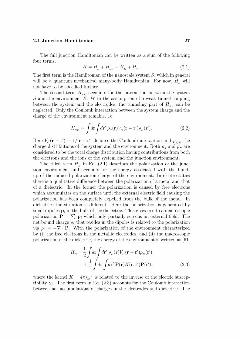
The starting point for the following analysis is a nanojunction consisting of ananoscale system S, e.g. a molecule, and the junction environment E whichusually consists of a number of metallic electrodes and a gate dielectric sep-arating the system from gate electrode. The situation is sketched in Fig. 2.1which illustrates the polarization and charge distribution of the junction fora positive gate voltage and charge Q = −e on the system S. In order tocalculate the position of the electronic levels of the system, the total energyof the system plus junction must be evaluated as a function of the chargeQ onthe system. This is a consequence of long ranged Coulomb interaction whichcouples the system charge with the polarization charge in the junction. Withall the microscopic degrees of freedom of the junction environment, this ofcourse posses an unsolvable problem. However, if the junction environmentis described with classical macroscopic electrostatics the problem simplifiesconsiderably. Within this approach the metallic electrodes are representedby equipotentials with their potentials given by the applied voltages Vi. Itis assumed that there is no net accumulation of charge in the junction envi-ronment, i.e. ρ
E= 0, when the junction is considered without the system S
and in the absence of applied voltages.
P+−
+−
+−
+−
+−
+−
+−
+−
+−
+−
+−
+−
+−
+−
+−
+−
+−
+−
+−
Gate
+−
+ + + + + + + +
− − −S
Q = −e
+++
+
++ +
+
− − −
s d
Figure 2.1: Schematic illustration of the charge distribution and polarizationP of the junction with a positive voltage applied to the gate electrode and thesource (s) and drain (d) electrodes grounded. The positive gate voltage has leftthe system S in the charge state QS = −e. The positive charges on the surface ofthe source and drain electrodes illustrates the polarization charge induced by theextra electron on the system.
2.1 Junction Hamiltonian 27
The full junction Hamiltonian can be written as a sum of the followingfour terms,
H = HS
+HSE
+HE
+HV. (2.1)
The first term is the Hamiltonian of the nanoscale system S, which in generalwill be a quantum mechanical many-body Hamiltonian. For now, H
Swill
not have to be specified further.The second term H
SEaccounts for the interaction between the system
S and the environment E. With the assumption of a weak tunnel couplingbetween the system and the electrodes, the tunneling part of H
SEcan be
neglected. Only the Coulomb interaction between the system charge and thecharge of the environment remains, i.e.
HSE
=
∫dr
∫dr′ ρ
S(r)V
C(r− r′)ρ
E(r′). (2.2)
Here VC(r − r′) = 1/|r − r′| denotes the Coulomb interaction and ρ
S/Ethe
charge distributions of the system and the environment. Both ρS
and ρE
areconsidered to be the total charge distribution having contributions from boththe electrons and the ions of the system and the junction environment.
The third term HE
in Eq. (2.1) describes the polarization of the junc-tion environment and accounts for the energy associated with the build-up of the induced polarization charge of the environment. In electrostaticsthere is a qualitative difference between the polarization of a metal and thatof a dielectric. In the former the polarization is caused by free electronswhich accumulates on the surface until the external electric field causing thepolarization has been completely expelled from the bulk of the metal. Indielectrics the situation is different. Here the polarization is generated bysmall dipoles pi in the bulk of the dielectric. This gives rise to a macroscopicpolarization P =
∑i pi which only partially screens an external field. The
net bound charge ρb
that resides in the dipoles is related to the polarizationvia ρb = −∇ · P. With the polarization of the environment characterizedby (i) the free electrons in the metallic electrodes, and (ii) the macroscopicpolarization of the dielectric, the energy of the environment is written as [61]
HE
=1
2
∫dr
∫dr′ ρ
E(r)V
C(r− r′)ρ
E(r′)
+1
2
∫dr
∫dr′ P(r)K(r, r′)P(r′), (2.3)
where the kernel K = 4πχ−1e is related to the inverse of the electric suscep-
tibility χe. The first term in Eq. (2.3) accounts for the Coulomb interactionbetween net accumulations of charges in the electrodes and dielectric. The

28 Electrostatics of single-molecule SETs
second term describes the elastic polarization energy of the dipoles pi whichis dominated by short ranged interactions. The polarization of the dielectricis connected to the electric field E via P = χeE. Since the energy of thepolarized dielectric is specified in terms of its macroscopic polarization, noassumption about the microscopic origin of the polarization is here required.However, it should be noted that an electrostatic description of the dynam-ical response of the junction environment relies on certain assumptions onthe time scale of the polarization response. A comment on this will follow inSec. 2.3.
In order to write the Hamiltonian of the environment in Eq. (2.3) asan interaction between the environmental charges ρ
E, the second term in
Eq. (2.3) is recast in the form of a density-density interaction between thebound polarization charges ρb,
1
2
∫dr
∫dr′ρb(r)Vb(r, r
′)ρb(r′). (2.4)
The interaction Vb between the bound charges is related to the kernel Kin Eq. (2.3) 1. For the present purpose a further specification of Vb is notnecessary. With this rearrangement the sum of the two terms in Eq. (2.3)can now be written
HE
=1
2
∫dr
∫dr′ ρ
E(r)V (r, r′)ρ
E(r′), (2.5)
where V is either VC
or VC
+Vb depending on whether r and r′ belong to themetallic and/or the dielectric parts of the environment.
Finally, the last term of the junction Hamiltonian in Eq. (2.1) is theenergy it costs to place a charge Qi on the i’th electrode which is held at thepotential Vi,
HV
=∑
i
QiVi. (2.6)
1Expressing the polarization in terms of the bound charge density via
P(r) = −∫dr′ r− r′
|r− r′|2ρb(r′),
the interaction between the bound charges Vb can be written as the following doubleintegral over the extend of the dielectric,
Vb(r, r′) =∫dr′′∫dr′′′ r− r′′
|r− r′′|2K(r′′, r′′′)
r′′′ − r′
|r′′′ − r′|2.

2.1 Junction Hamiltonian 29
The charge on the i’th electrode is given by the spatial integral of ρE
overthe extend of the electrode, Qi =
∫r∈idr ρ
E(r). With the different parts of
the junction Hamiltonian in Eq. (2.1) specified it now takes the form
H = HS
+ ρSV
SEρ
E+
1
2ρ
EV
EEρ
E+∑
i
QiVi, (2.7)
where the shorthand notation Vmnρn =∫dr′V (r, r′)ρ(r′) with m,n = S,E
has been introduced for brevity. The subscripts in Eq. (2.7) indicate whichpart of the junction the spatial variable belongs to. In the following it isshown how an explicit treatment of the degrees of freedom of the environmentcan be avoided.
For a given charge distribution ρS
of the system and applied voltages Vi
to the electrodes, the environment will polarize in order to lower the totalenergy. Since the part of the Hamiltonian involving ρ
Eis treated classically
here, the solution for ρE
can be found by minimizing the Hamiltonian inEq. (2.7) with respect to ρ
E. This yields the following expression for charge
distribution of the junction environment
ρE
= −[VEE
]−1
(V
ESρ
S+∑
i
Vi
)≡ ρind + ρext. (2.8)
Two contributions are here identified. The first denoted ρind, represents thepolarization charge induced by the system charge ρ
S. In linear response the-
ory the response function χ relates the induced charge density to an externalpotential,
ρind(r) =
∫dr′χ(r, r′)Φ(r′). (2.9)
In Eq. (2.8) above, the potential from the system charge ΦS
= VESρ
Stakes
the role of the external potential. Therefore, the inverse of the interaction VEE
can be identified as the linear response function of the junction, χ = −V −1EE
.
The second contribution ρext to the charge distribution of the environmentin Eq. (2.8), represents the charge induced in the junction when externalvoltages Vi are applied to the electrodes. This consists of the charge that issupplied by an external battery in order to maintain the applied voltages,plus the charge that results from the polarization of the dielectric that followsa finite voltage applied to one or more of the electrodes (see e.g. Fig. 2.1).
With the expression for ρE
in Eq.(2.8) inserted back into the Hamiltonian
30 Electrostatics of single-molecule SETs
in Eq. (2.7), the following effective junction Hamiltonian is obtained,
H = HS− 1
2ρ
SV
SE[V
EE]−1V
ESρ
S−∑
i
Vi[VEE]−1V
ESρ
S
− 1
2
∑ij
Vi[VEE]−1Vj
= HS
+1
2
∫dr
∫dr′ ρ
S(r)V (r, r′)ρ
S(r′) +
∫dr ρ
S(r)Φext(r)
+1
2
∑ij
ViCijVj
≡ HS
+Hpol +Hext +HC. (2.10)
The elimination of the charge density of the environment ρE
has resultedin the appearance of new quantities in the Hamiltonian. These are definedby the second equality where the real space notation has been reintroduced.Firstly, an effective interaction
V = −VSE
[VEE
]−1VES
(2.11)
between the system charges has been identified. As will be discussed inSec. 2.1.2, this interaction is mediated by the induced polarization charge.Secondly, the electrostatic potential Φ(r)ext =
∫dr′V
C(r−r′)ρext(r
′) from thecharge distribution ρext in Eq. (2.8) has been introduced. Last, the elementsCij of the capacitance matrix are identified as
Cij = −∫
r∈i
dr
∫r′∈j
dr′ V −1(r, r′), (2.12)
where the integration extends over the volume of the i’th and j’th electrodeand V is the interaction in the environment from Eq. (2.5). As the inverseV −1 of the interaction is related to the response function, the capacitancematrix is fully determined by the geometry of the junction and its dielectricproperties.
Each of the terms in the effective Hamiltonian in Eq. (2.10) accounts forwell defined contributions to the total energy. Starting with the last term,H
Cis the electrostatic energy of the junction in the absence of the system
S and with voltages Vi applied to the electrodes. This part of the electro-static energy is provided by a battery and has no influence on the electroniclevels of the system. The term Hext, is the energy of the system charge ρ
S
in the potential from the applied voltages. The capacitive coupling to thegate electrode is described by this term. The polarization Hamiltonian Hpol
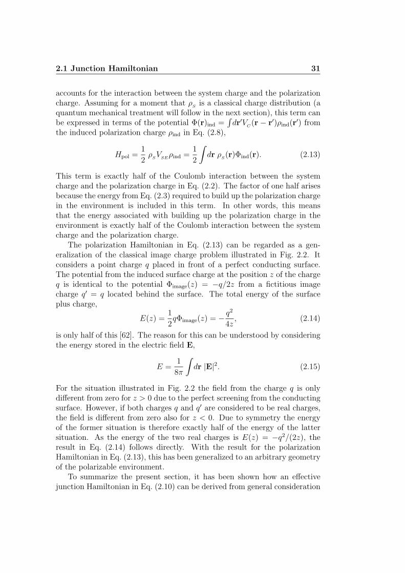
2.1 Junction Hamiltonian 31
accounts for the interaction between the system charge and the polarizationcharge. Assuming for a moment that ρ
Sis a classical charge distribution (a
quantum mechanical treatment will follow in the next section), this term canbe expressed in terms of the potential Φ(r)ind =
∫dr′V
C(r − r′)ρind(r
′) fromthe induced polarization charge ρind in Eq. (2.8),
Hpol =1
2ρ
SV
SEρind =
1
2
∫dr ρ
S(r)Φind(r). (2.13)
This term is exactly half of the Coulomb interaction between the systemcharge and the polarization charge in Eq. (2.2). The factor of one half arisesbecause the energy from Eq. (2.3) required to build up the polarization chargein the environment is included in this term. In other words, this meansthat the energy associated with building up the polarization charge in theenvironment is exactly half of the Coulomb interaction between the systemcharge and the polarization charge.
The polarization Hamiltonian in Eq. (2.13) can be regarded as a gen-eralization of the classical image charge problem illustrated in Fig. 2.2. Itconsiders a point charge q placed in front of a perfect conducting surface.The potential from the induced surface charge at the position z of the chargeq is identical to the potential Φimage(z) = −q/2z from a fictitious imagecharge q′ = q located behind the surface. The total energy of the surfaceplus charge,
E(z) =1
2qΦimage(z) = − q
2
4z, (2.14)
is only half of this [62]. The reason for this can be understood by consideringthe energy stored in the electric field E,
E =1
8π
∫dr |E|2. (2.15)
For the situation illustrated in Fig. 2.2 the field from the charge q is onlydifferent from zero for z > 0 due to the perfect screening from the conductingsurface. However, if both charges q and q′ are considered to be real charges,the field is different from zero also for z < 0. Due to symmetry the energyof the former situation is therefore exactly half of the energy of the lattersituation. As the energy of the two real charges is E(z) = −q2/(2z), theresult in Eq. (2.14) follows directly. With the result for the polarizationHamiltonian in Eq. (2.13), this has been generalized to an arbitrary geometryof the polarizable environment.
To summarize the present section, it has been shown how an effectivejunction Hamiltonian in Eq. (2.10) can be derived from general consideration
32 Electrostatics of single-molecule SETs
q+z
e−
+ +
+ +
+ + E
−zq’
Figure 2.2: The classical image charge problem with a charge q = −e located ata distance z from a perfect conducting surface. The effect of the positive surfacecharge is equivalent to a fictitious image charge q′ = −q behind the metal surface.
on the electrostatic energy of the junction. In the resulting Hamiltonianthe charge distribution of the junction environment has been replaced bymacroscopic quantities describing the mutual interaction between the chargesof the environment and their interaction with the system. These include aneffective interaction V between the system charges, the potential Φext fromthe charge ρext which is added to the electrodes to maintain the appliedvoltages Vi, and the elements Cij of the capacitance matrix of the junction.
2.1.1 Quantum mechanical version
For systems where the electronic degrees of freedom are governed by theSchrodinger equation, a quantum mechanical version of the effective junctionHamiltonian in Eq. (2.10) is required.
In its most general form the Hamiltonian of the system will be a many-body Hamiltonian consisting of a non-interaction part H0 including the ki-netic energy of the electrons and the potential from the ionic cores of thesystem, and an interacting part Hint which describes the Coulomb interactionbetween the electrons,
HS
=H0 +Hint
=− 1
2
∫dr ψ†(r)∇2ψ(r) +
∫dr ψ†(r)ψ(r)Vion(r)
+1
2
∫dr
∫dr′ ψ†(r)ψ†(r′)V
C(r− r′)ψ(r′)ψ(r). (2.16)
Here ψ† and ψ denote the creation and annihilation field operators and
2.1 Junction Hamiltonian 33
Vion(r) = −∫drV
C(r−r′)ρion(r
′) is the energy of the electrons in the potentialfrom the ionic cores. To ease the notation, the electronic spin variable hasbeen suppressed in Eq. (2.16) and in the remainder of this chapter.
The quantum mechanical version of the effective junction terms inEq. (2.10) follows by replacing the charge distribution of the system by itscontributions from the ionic cores and the electrons with the latter repre-sented by the electronic field operators, i.e. ρ
S= ρion − ψ†ψ. The term Hext
accounting for the applied voltages takes the form
Hext =
∫dr[ρion(r)− ψ†(r)ψ(r)
]Φext(r). (2.17)
Under the assumption that the ionic cores of the system S remain fixed asa function of applied voltages and number of electrons on the system, thefirst term affects only the zero point of the total energy and can hence beneglected. The single-particle contribution in the other term adds to thenon-interaction part H0 of the system Hamiltonian. It affects the eigenstatesand hence also the electronic charge distribution of the system when voltagesare applied to the electrodes. Furthermore, this term accounts for the shiftof the electronic levels due to an applied gate voltage.
The quantum mechanical version of the polarization Hamiltonian Hpol isgiven by
Hpol =1
2
∫dr
∫dr′ ρion(r)V (r, r′)ρion(r
′)
−∫dr
∫dr′ ψ†(r)ψ(r)V (r, r′)ρion(r
′)
+1
2
∫dr
∫dr′ ψ†(r)ψ(r)V (r, r′)ψ†(r′)ψ(r′), (2.18)
where V is the effective interaction between the system charges fromEq. (2.11). Again, the term involving the ionic charge distribution ρion canbe neglected under the assumption that the ionic cores remain fixed. Thesecond term contains the interaction between the electrons and the imagecharges of the ions and visa versa. This is a single-particle term that adds toH0 as above. The last term, which in the following will be denoted H int
pol, de-scribes the interaction between the electrons and their image charges. Exceptfor the ordering of the field operators and the substitution of the Coulombinteraction V
Cwith the effective interaction V , this term is equivalent to the
interaction part Hint of the system Hamiltonian in Eq. (2.16). Due to thedifferent ordering of the field operators in H int
pol, this term includes contribu-tions where the electrons interact with themselves. This self-interaction is a

34 Electrostatics of single-molecule SETs
consequence of the fact that an electron can interact with itself via its ownimage charge. By reordering the field operators, the self-interaction of theelectrons can be separated out in an extra single-particle term
H intpol =
1
2
∫dr ψ†(r)ψ(r)V (r, r)
+1
2
∫dr
∫dr′ ψ†(r)ψ†(r′)V (r, r′)ψ(r′)ψ(r). (2.19)
The last term now has the same ordering of the field operators as the Coulombinteraction term Hint in the system Hamiltonian. Consequently, the polariza-tion of the environment modifies the interaction on the system by replacingthe bare Coulomb interaction with a screened interaction Vscr = V
C+ V . On
top of this, the polarization Hamiltonian introduced two new single-particleterms (the second term in Eq.(2.18) and the first term in Eq. (2.19)). Ex-cept for the self-interaction term in Eq. (2.19), all terms in the polarizationHamiltonian have equivalent counterparts in the system Hamiltonian H
S
in Eq. (2.16) with V replaced by the Coulomb interaction VC. They can
therefore be joined and expressed in terms of the screened interaction Vscr.The full quantum mechanical version of the effective junction Hamiltonianin Eq. (2.10) then takes the form
H =− 1
2
∫dr ψ†(r)∇2ψ(r) +
∫dr ψ†(r)ψ(r)Vext(r)
−∫dr
∫dr′ ψ†(r)ψ(r)Vscr(r, r
′)ρion(r′)
+1
2
∫dr
∫dr′ ψ†(r)ψ†(r′)Vscr(r, r
′)ψ(r′)ψ(r)
+1
2
∫dr ψ†(r)ψ(r)V (r, r), (2.20)
where the terms not depending on the electronic degrees of freedom havebeen neglected. This Hamiltonian provides a general starting point for adescription of the electronic structure of a system which is weakly coupledto the metallic electrodes of a nanoscale junction. Since it is merely a modi-fication of the terms contained in the Hamiltonian of the isolated system inEq. (2.16), the junction Hamiltonian can be tackled with existing methodsfor many-body eigenvalue problems. These range from exact diagonalizationto mean-field treatments in the Hartree and Hartree-Fock approximation. InSec. 2.2 the version of the junction Hamiltonian suitable for effective single-particle descriptions such as e.g. density functional theory, is presented.
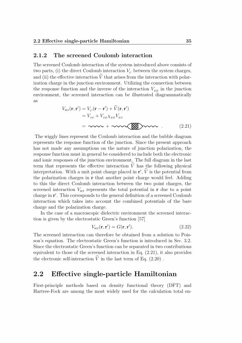
2.2 Effective single-particle Hamiltonian 35
2.1.2 The screened Coulomb interaction
The screened Coulomb interaction of the system introduced above consists oftwo parts, (i) the direct Coulomb interaction V
Cbetween the system charges,
and (ii) the effective interaction V that arises from the interaction with polar-ization charge in the junction environment. Utilizing the connection betweenthe response function and the inverse of the interaction V
EEin the junction
environment, the screened interaction can be illustrated diagrammaticallyas
Vscr(r, r′) = V
C(r− r′) + V (r, r′)
= VSS
+ VSEχ
EEV
ES
=
+
. (2.21)
The wiggly lines represent the Coulomb interaction and the bubble diagramrepresents the response function of the junction. Since the present approachhas not made any assumptions on the nature of junction polarization, theresponse function must in general be considered to include both the electronicand ionic responses of the junction environment. The full diagram in the lastterm that represents the effective interaction V has the following physicalinterpretation. With a unit point charge placed in r′, V is the potential fromthe polarization charges in r that another point charge would feel. Addingto this the direct Coulomb interaction between the two point charges, thescreened interaction Vscr represents the total potential in r due to a pointcharge in r′. This corresponds to the general definition of a screened Coulombinteraction which takes into account the combined potentials of the barecharge and the polarization charge.
In the case of a macroscopic dielectric environment the screened interac-tion is given by the electrostatic Green’s function [57]
Vscr(r, r′) = G(r, r′). (2.22)
The screened interaction can therefore be obtained from a solution to Pois-son’s equation. The electrostatic Green’s function is introduced in Sec. 3.2.Since the electrostatic Green’s function can be separated in two contributionsequivalent to those of the screened interaction in Eq. (2.21), it also provides
the electronic self-interaction V in the last term of Eq. (2.20) .
2.2 Effective single-particle Hamiltonian
First-principle methods based on density functional theory (DFT) andHartree-Fock are among the most widely used for the calculation total en-

36 Electrostatics of single-molecule SETs
ergies of molecules. Therefore, a reformulation of the junction Hamiltonianin Eq. (2.20) to an effective single-particle Hamiltonian is of high practicalrelevance.
In effective single-particle descriptions the electrons are treated as non-interacting moving in an effective potential that accounts for the electron-electron interactions at the level of mean-field theory. The difference betweenvarious single-particle descriptions lies in their approximation to the effectivesingle-particle potential Veff.
Without loss of generality an effective single-particle Hamiltonian can bewritten as
Heff = −1
2∇2 + Veff(r) (2.23)
with the effective potential given by the sum of the following contributions
Veff(r) = Vion(r) + VH(r) + Vxc(r) + Vind(r) + Vext(r). (2.24)
The first three terms of the effective potential originate from the moleculeitself. They include the potential Vion from the ionic cores, the Hartreepotential from the electron density ne,
VH(r) =
∫dr′ V
C(r− r′)ne(r
′), (2.25)
and the exchange-correlation potential Vxc which accounts for the part ofthe electron-electron interactions not included in the Hartree potential. Thiscould be e.g. the exchange-correlation potential from the Kohn-Sham Hamil-tonian in DFT or the non-local exchange potential of Hartree-Fock [63]. Thefourth term describes the interaction with the polarization charge through theinduced potential Vind. It follows from a Hartree approximation to the imagecharge mediated electron-electron interactions in the polarization Hamilto-nian in Eq. (2.18). Since self-interactions are included in this interaction, theHartree approximation captures the essential physics of this term. It shouldbe noted that Vind = Vind,e + Vind,ion is the sum of the potentials induced bythe electrons and the ionic cores of the molecule. The last contribution tothe effective potential in Eq. (2.24) accounts for the potential from appliedvoltages.
The electron density is obtained by occupying the lowest lying eigenfunc-tion φi of the effective Hamiltonian in Eq. (2.23)
ne(r) =∑i∈occ
|φi(r)|2. (2.26)
As the effective potential depends on the electron density, the eigenfunctionsand their corresponding energies εi must be determined self-consistently by

2.3 Validity of an electrostatic approach 37
updating the effective potential from the electron density in each iteration.The self-consistent scheme allows the electron density of the molecule torelax in response to the junction polarization and applied voltages which arerepresented by the induced potential Vind and the external potential Vext,respectively. As a consequence, the molecular orbitals φi might change qual-itatively compared to those of the isolated molecule.
From the eigenvalues of the effective Hamiltonian the total energy can beobtained as
E =∑i∈occ
εi −1
2
∫dr ne(r) [VH(r) + Vind,e(r)] + ∆xc. (2.27)
Here the second term prevents double counting contributions to the totalenergy which are included twice in the sum of the eigenvalues. Notice thatthis term includes only the induced potential Vind,e from the electronic chargeand not the full induced potential Vind. The last term ∆xc, which accountsfor the exchange-correlation part of the total energy, depends on the differentsingle-particle descriptions.
The results presented in this thesis are based on the semi-empiricalmethod outlined in App. B. It is based on the extended Huckel scheme whichfor the present purpose has been extended with a self-consistent field tak-ing into account electron-electron interactions at the level of Hartree theory.The potentials Vind and Vext are obtained from a finite element solution toPoisson’s equation. The next chapter introduces Poisson’s equation and thefinite element method.
2.3 Validity of an electrostatic approach
The derivation of the effective junction Hamiltonian in Eq. (2.20) relies onthe assumption that the junction environment can be described by a classi-cal electrostatic Hamiltonian. Below it is discussed which requirements thisimposes on the size of the junction constituents and the time scales of thejunction polarization.
First of all, the classical treatment is based on the macroscopic dielectricproperties of the junction environment. Therefore, the dimensions of the elec-trodes and dielectric must be sufficiently large that these can be defined. Forthe metallic electrodes which are assumed to be equipotentials, this impliesthat their size must be larger than the metallic screening length. With typicalmetallic screening lengths being on the order of 1 − 2 A [62], this is readilyfulfilled. The macroscopic polarization P of a dielectric follows by averagingthe microscopic fluctuations over a suitable volume. For a crystalline solid

38 Electrostatics of single-molecule SETs
this is the unit cell. Hence, the dimensions of the dielectric components of thejunction must be larger than the unit cell dimensions. As the gate dielectricin single-molecule SETs is on the order of nanometers, this is also fulfilled.
Secondly, the assumption of an electrostatic environment neglects dynam-ical polarization effects. For this to hold the dynamics of the polarizationresponse need to be the fastest time scale in the problem such that theenvironment can be assumed to responds instantaneously to changes in thenumber of electrons on the molecule. Based on the time-scale discussion inSec. 1.3.3 which introduced the junction polaron concept, this seems to bewell justified. An electrostatic approach is therefore a good starting pointfor studying polarization effects in single-molecule SETs.
There is another time scale associated with the electron dynamics inter-nally on the molecule. It is given by the energy of the molecular gap which ison the order of ∼ eV. For time scales faster than the one set by the molecu-lar gap the molecular orbitals of an effective single-particle approach are notwell-defined. As the time scale given by the inverse of the plasmon frequencyis also on the order of eV, this implies that a single-particle description ofthe polarization effects does not necessarily give a correct description of themolecular wavefunction. Alternatively, the problem should be attacked in itsmany-body form in Eq. (2.20) which takes into account the image chargesof the electronic point charges instead of the image charge of the molecularorbitals. However, as a first iteration of the study of polarization effects insingle-molecule SETs, the effective single-particle description adopted in thepresent work can be expected to give the order of magnitude of the effect onthe molecular levels.
Chapter 3
Poisson’s equation
The spatial profile of the electrostatic potential in the nanoscale gap of asingle-molecule SET is an important factor for its transistor related proper-ties. Therefore, the solution of Poisson’s equation in a realistic 3-dimensionalgeometry is a compulsory part in the characterization of the electrostaticproperties of single-molecule SETs. The following chapter discusses the dif-ferent contributions to the electrostatic potential in a single-molecule junc-tion. Furthermore, the numerical finite element method for the solution ofPoisson’s equation is introduced.
3.1 Junction potential
The electrostatic potential Φ in a nanojunction is given Poisson’s equation
−∇ · [εr(r)∇Φ(r)] = 4πρS(r) (3.1)
with boundary conditions given by the voltages applied to the electrodes
Φ(r)|r∈Si= Vi. (3.2)
Here Si denotes the surface of the i’th electrode with potential Vi. The screen-ing properties of the junction are included via the spatially dependent dielec-tric constant εr and ρ
Sis the charge distribution of the system/molecule.
Due to the superposition principle the total potential of the junction canbe split up in a part Φ
Sdescribing the part of the potential that stems from
the presence of the charge distribution ρS
and a part Φext associated withthe applied voltages Vi,
Φ(r) = ΦS(r) + Φext(r). (3.3)
40 Poisson’s equation
The potential ΦS
obeys the Poisson equation in Eq. (3.1) with boundaryconditions Φ(r) = 0 for r ∈ Si. The remaining part of the total potential isthe potential from the applied voltages in the absence of the system chargeρ
Swhich can be expressed by the sum
Φext(r) =∑
i
αi(r)Vi (3.4)
where the characteristic electrode functions αi are determined by Laplace’sequation
∇ · [εr(r)∇αi(r)] = 0 (3.5)
with boundary conditions αi(r) = δij for r ∈ Sj. The characteristic functionsαi represent the electrostatic potential of the junction with a unit potentialapplied to electrode i and all other electrodes grounded.
The potential ΦS
arising due to the presence of the system charge isthe sum of the potential Φ′
Sfrom the system charge itself when considered
without the junction and the potential Φind from the induced polarizationcharge ρind in the junction
ΦS(r) = Φ′
S(r) + Φind(r). (3.6)
Each of the potentials on the right-hand side follows from their correspondingcharge distributions
Φ(r) =
∫dr′ V
C(r− r′)ρ(r′). (3.7)
In the following two sections methods for solving Poisson’s equation are in-troduced. While a formal solution can be obtained with the aid of the elec-trostatic Green’s function, in practice, one must often resort to numericalmethods such as the finite element method.
3.2 Electrostatic Green’s function
The electrostatic Green’s function solves Poisson’s equation with a δ-functionsource term
−∇ · [εr(r)∇G(r, r′)] = 4πδ(r− r′) (3.8)
and boundary conditionsG(r, r′)|r∈Si
= 0. (3.9)
Its interpretation is that it gives the potential at position r due to a unit pointcharge in r′. Consequently, the Green’s function is fully determined by the
3.2 Electrostatic Green’s function 41
screening properties and the geometry of the junction. As the potential ΦS
inEq. (3.6) the Green’s function can be written as the sum of two contributions
G(r, r′) =1
|r− r′|+ G(r, r′). (3.10)
The first term is the bare potential from the point charge in r′ and thesecond term is the induced junction potential. Notice that the contributionG is equivalent to the effective interaction V in Eq. (2.21).
The Green’s function gives a formal solution to Poisson’s equation for thepotential Φ
Svia
ΦS(r) =
∫dr′ G(r, r′)ρ
S(r′). (3.11)
That this is in fact a solution can be readily confirmed by inserting in Pois-son’s equation (3.1) and utilizing that the Green’s function is the solution toEq. (3.8). Also, the characteristic electrode functions αi can be expressed interms of the Green’s function as [64]
αi(r) = −∫
Si
dS ′ εr(r)n · ∇′G(r, r′), (3.12)
where n is an outward pointing normal to the electrode surface Si.
3.2.1 Analytical solution in simplified junction
In the following an analytic solution for the Green’s function in the simplifiedjunction geometry shown in Fig. 3.1 is given. Despite its simple appearance,this junction resembles the screening properties of more realistic junctiongeometries rather well. The electrodes are represented by infinite parallelmetal surfaces with the dielectric material filling the lower half of the spacingbetween them.
Consider a unit point charge located in r′ = (x′, y′, z′) in the spacingbetween the electrodes and dielectric. The presence of the point charge in-duces a polarization in the junction. At the surface of the metallic electrodesthe potential from the induced charge cancels the potential from the pointcharge. This results in the boundary condition in Eq. (3.9) for the Green’sfunction at the electrode surfaces. At the dielectric interface the cancellationof the point charge potential is only partial. The potential can be obtainedby solving Eq. (3.8) where the dielectric constant εr describes the screeningof the dielectric. Alternatively, the induced charge of the dielectric can betreated as a source term on equal footing with the point charge. With theinduced charge included explicitly as a source term, Poisson’s equation must
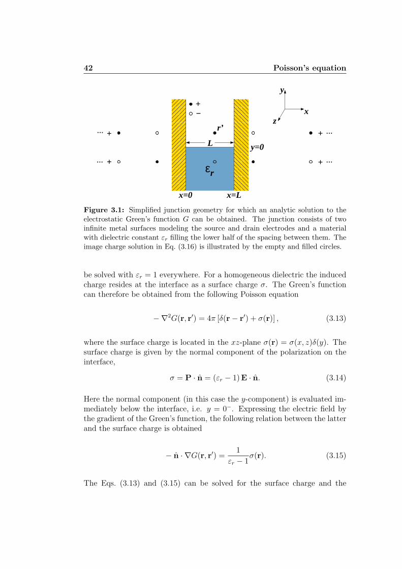
42 Poisson’s equation
... +
... +
...+
...+
+−
L
x
y
z
y=0
r’
x=0 x=L
εr
Figure 3.1: Simplified junction geometry for which an analytic solution to theelectrostatic Green’s function G can be obtained. The junction consists of twoinfinite metal surfaces modeling the source and drain electrodes and a materialwith dielectric constant εr filling the lower half of the spacing between them. Theimage charge solution in Eq. (3.16) is illustrated by the empty and filled circles.
be solved with εr = 1 everywhere. For a homogeneous dielectric the inducedcharge resides at the interface as a surface charge σ. The Green’s functioncan therefore be obtained from the following Poisson equation
−∇2G(r, r′) = 4π [δ(r− r′) + σ(r)] , (3.13)
where the surface charge is located in the xz-plane σ(r) = σ(x, z)δ(y). Thesurface charge is given by the normal component of the polarization on theinterface,
σ = P · n = (εr − 1)E · n. (3.14)
Here the normal component (in this case the y-component) is evaluated im-mediately below the interface, i.e. y = 0−. Expressing the electric field bythe gradient of the Green’s function, the following relation between the latterand the surface charge is obtained
− n · ∇G(r, r′) =1
εr − 1σ(r). (3.15)
The Eqs. (3.13) and (3.15) can be solved for the surface charge and the
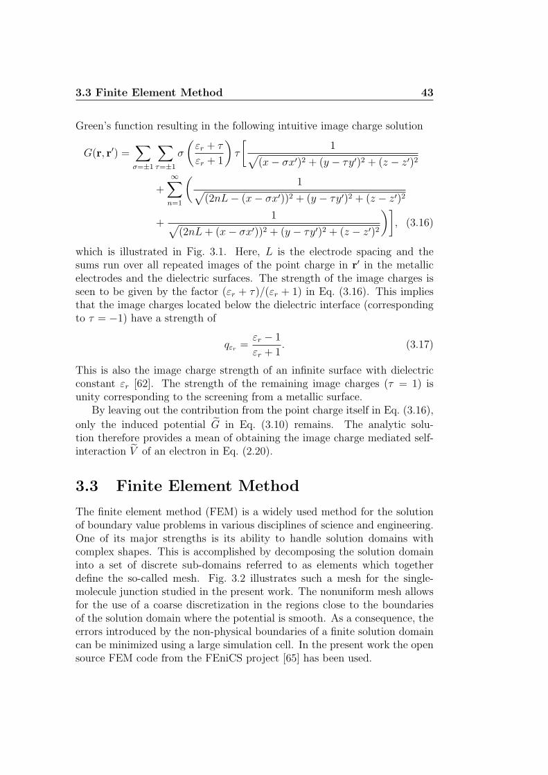
3.3 Finite Element Method 43
Green’s function resulting in the following intuitive image charge solution
G(r, r′) =∑σ=±1
∑τ=±1
σ
(εr + τ
εr + 1
)τ
[1√
(x− σx′)2 + (y − τy′)2 + (z − z′)2
+∞∑
n=1
(1√
(2nL− (x− σx′))2 + (y − τy′)2 + (z − z′)2
+1√
(2nL+ (x− σx′))2 + (y − τy′)2 + (z − z′)2
)], (3.16)
which is illustrated in Fig. 3.1. Here, L is the electrode spacing and thesums run over all repeated images of the point charge in r′ in the metallicelectrodes and the dielectric surfaces. The strength of the image charges isseen to be given by the factor (εr + τ)/(εr + 1) in Eq. (3.16). This impliesthat the image charges located below the dielectric interface (correspondingto τ = −1) have a strength of
qεr =εr − 1
εr + 1. (3.17)
This is also the image charge strength of an infinite surface with dielectricconstant εr [62]. The strength of the remaining image charges (τ = 1) isunity corresponding to the screening from a metallic surface.
By leaving out the contribution from the point charge itself in Eq. (3.16),
only the induced potential G in Eq. (3.10) remains. The analytic solu-tion therefore provides a mean of obtaining the image charge mediated self-interaction V of an electron in Eq. (2.20).
3.3 Finite Element Method
The finite element method (FEM) is a widely used method for the solutionof boundary value problems in various disciplines of science and engineering.One of its major strengths is its ability to handle solution domains withcomplex shapes. This is accomplished by decomposing the solution domaininto a set of discrete sub-domains referred to as elements which togetherdefine the so-called mesh. Fig. 3.2 illustrates such a mesh for the single-molecule junction studied in the present work. The nonuniform mesh allowsfor the use of a coarse discretization in the regions close to the boundariesof the solution domain where the potential is smooth. As a consequence, theerrors introduced by the non-physical boundaries of a finite solution domaincan be minimized using a large simulation cell. In the present work the opensource FEM code from the FEniCS project [65] has been used.

44 Poisson’s equation
In general, the boundary value problem for Poisson’s equation in thesolution domain Ω defined by the junction geometry can be formulated as
−∇ · [εr∇u] = f, r ∈ Ω (3.18)
u = g, r ∈ ∂ΩD (3.19)
n · ∇u = h, r ∈ ∂ΩN (3.20)
In the more general notation introduced here, u denotes the electrostaticpotential, f = 4πρ is the source term, and g and h are scalar functionsspecifying the value of the potential and its normal derivative on the Dirichletand Neumann parts of the boundary, respectively.
Instead of the differential form above, the finite element method takes itsstarting point in the variational formulation of the boundary value problem.To rewrite the differential boundary value problem to its variational form,Eq. (3.18) is multiplied with an arbitrary test function v belonging to thefunction space V in which the solution is sought. Subsequently, the equationis integrated over the solution domain Ω and using integration by parts thevariational form follows∫
Ω
dr εr∇v · ∇u =
∫Ω
dr vf +
∫∂Ω
dS εrv (n · ∇)u. (3.21)
The boundary integral on the right-hand side is handled by inserting theNeumann boundary condition from equation (3.20). The fact that only firstorder derivatives appears, ensures that the variational formulation is well-defined as long as v and u are continuous piecewise differentiable functions.Since such functions do not have continuous first derivatives as required bythe differential form of Poisson’s equation, the variational formulation is alsoreferred to as the weak form and its solution a weak solution. Introducingthe bilinear form
a(v, u) =
∫Ω
dr εr∇v · ∇u (3.22)
and linear form
b(v) =
∫Ω
dr vf (3.23)
on V , then for u to be a solution
a(v, u) = b(v) ∀v ∈ V. (3.24)
From the variational form of the boundary value problem, the next stepis the discretization in the finite element space which is composed of basis
3.3 Finite Element Method 45
Figure 3.2: Boundary mesh of the 3-dimensional simulation cell for a single-molecule junction. The nonuniform mesh allows to obtain an accurate representa-tion of the potential in the relevant region near the molecule while at the same timeminimizing the errors due to non-physical boundaries by using a large simulationcell.
functions φi with compact support. The most simple basis is the linear basisfunction which for each node (element vertex) of the mesh connects to theneighboring nodes with a linear function with value one at the node itselfand zero at the neighboring nodes (hence the compact support). In the finiteelement basis the solution u is expanded as
u =∑
i
uiφi (3.25)
where φiNi=1 is the global basis of the finite element space. The expansion is
then substituted into the weak formulation and the test function v is chosento coincide with a basis function φi. This particular approach is often referredto as Galerkin finite element discretization. The resulting algebraic systemcan be written in matrix form as
Ku = f (3.26)
where u is a vector holding the expansion coefficients in Eq. (3.25), Kij =a(φi, φj) and the elements of the right-hand side are given by fi = b(φi)where a and b are the bilinear and linear forms defined above in Eqs. (3.22)and (3.23). The assembly and the solution of the matrix equation inEq. (3.26) are the time-consuming parts of a FEM calculations. Dependingon the size N of the linear system it can be tackled with either direct oriterative methods [66].


Chapter 4
Characterization of an OPV5SET
Single-molecule SETs based on the conjugated oligo-phenylene vinylene(OPVs) molecules have been subject to a number of studies over the recentyears [20, 36, 49, 50]. The experiment published in Ref. [20] was the firstto report access to several charge states of a molecule in a single-moleculeSET. The measured stability diagram (see Fig. 1.9) showed diamonds ofvarying size. This serves as a fingerprint of the quantization of the molecu-lar levels. Interestingly, the gap of the OPV5 molecule extracted from thestability diagram was strongly reduced (∼ 300 meV) compared to its valuein electrochemical experiments (∼ 2.5 eV). This effect, which has been ob-served consistently for various single-molecules SETs, been ascribed to imagecharges in the metallic electrodes [58]. So far, however, no satisfactory ex-planation of the effect in single-molecule SETs has been given. As the imagecharge effect is strongly dependent on the geometry of the junction and theposition of the molecule in the junction, a quantitative estimate requires a 3-dimensional simulation of the junction combined with an atomic descriptionof the molecule.
To date, only a few theoretical studies of single-molecule SETs basedon an atomic description of the molecule and a realistic junction geometryhave been reported in the literature. They have focused on the vibrationalproperties of the OPV5 molecule in the junction [67] and image charge effectsin a simplified junction geometries [58, 60]. The purpose of the presentchapter is to study the effect of image charges/junction polarization in arealistic OPV5-based single-molecule junctions with the formalism developedin Chap. 4. Furthermore, some general aspects such as the gate coupling tothe molecule and the effect of a finite source-drain voltage will be addressed.

48 Characterization of an OPV5 SET
4.1 OPV5 SET
The simulated OPV5 SET is illustrated in Fig. 4.1. It has the moleculestretched out between the source and drain electrodes which are separatedby a ∼ 3.2 nm gap. Without the molecule, the junction is taken to betranslation invariant in the direction parallel to the electrode edges. In orderto resemble the experimental settings [20], the molecule is separated fromthe gate electrode by a 5 nm thick gate dielectric with dielectric constantεr = 10. This corresponds to the high-κ dielectric Al2O3 [2]. The relativelyhigh dielectric constant of the gate dielectric ensures a reasonable capacitivecoupling between the gate and the molecule. The source and drain electrodesin Fig. 4.1 have been cutoff in the vertical direction for visual reasons. Inthe numerical simulations they are modelled by infinitely high metal blockswith potentials given by the applied voltages. The molecule is positionedflat on top of the gate dielectric with a distance of 1 A to the surfaces of thesource/drain electrodes and the gate dielectric. With the electrostatic imageplane located outside the atomic surfaces [68, 69], this effectively correspondsto a distance on the order of a van der Waals distance (∼ 3 A) between themolecule and the surface atoms.
The molecular structure of the OPV5 molecule is shown in the right sideof Fig. 4.1 together with the HOMO and LUMO orbitals. To resemble themolecule used in experiments [20], a thiol group (SH) is attached to theterminating phenylene units. The thiol group localizes the HOMO on theterminating phenylene unit. Furthermore, it donates electrons the π-systemon the carbon backbone of the molecule, which result in a net positive chargeof the thiol group. In all calculations presented in the following the molecule
OPV5
LUMO
HOMO
Figure 4.1: OPV5-SET and molecular orbitals. (left) Geometry of the simulatedOPV5-SET. The OPV5 molecule is stretched out between the electrodes whichare separated by ∼ 3.2 nm. (right) Structure and HOMO/LUMO orbitals of thethiol-terminated OPV5 molecule.
4.2 Polarization effects 49
will be considered in neutral state geometry.In this chapter the positions of the molecular levels are studied as a
function of different junction properties and applied voltages to the source,drain and gate electrodes. For this purpose the total energy is evaluatedfor the different charge states of the molecule, i.e. with varying numberof electrons on the molecule. The molecular ionization potential (IP) andelectron affinity (EA) are given by the difference in total energy between theneutral and singly charged states of the molecule, i.e.
IP = EN−1 − EN and EA = EN − EN+1. (4.1)
Here, N denotes the number of electrons in the neutral state of the molecule.The charged states with one electron added (N + 1) and removed (N − 1),correspond to the anion and cation, respectively. The molecular gap is givenby the difference between the ionization potential and electron affinity,
Egap = IP− EA = EN−1 + EN+1 − 2EN . (4.2)
In the following the effect of junction polarization is quantified in terms ofthe polarization energy P which gives the reduction of the gap relative to itsgas phase (g) value, i.e. Egap = Egap(g) − P . It can be regarded as a sumof the polarization energies of the negatively and positively charged statesof the molecule, P = P+ + P− (see Fig. 1.7). The physical interpretation ofthe polarization energies P+/− is that they give the total gain in energy uponintroducing the charged molecule in the junction.
In the present work a self-consistent Huckel implementation of the effec-tive junction Hamiltonian in Eq. (2.23) is used to calculate the total energies.The details of the Huckel implementation is outlined in App. B. It should benoted that the self-consistent Huckel method underestimates the moleculargaps as compared to DFT. However, since the change in the gap due to theinteraction with the polarization charge is relatively independent on the sizeof the gap, this should not have any significant influence on the conclusionsdrawn here.
4.2 Polarization effects
The present section studies the effect of junction polarization in the ab-sence of applied voltages. The polarization of the junction is illustratedin Fig. 4.2 which shows contour plots of the induced potential Φind for theneutral molecule and the negatively charged anion. From the induced po-tential it is clear that the negative charge of the anion results in a significant

50 Characterization of an OPV5 SET
Figure 4.2: Illustration of the polarization response of the junction showingcontour plots of the induced potential Φind at the surfaces of the electrodes andgate dielectric. (left) Neutral OPV5 molecule. (right) Negatively charged anion.
polarization of the junction. The polarization due to the neutral moleculeis less pronounced. However, the positively charged thiol groups induces anegative potential in their vicinity which results in an increased polarizationof the molecule during the self-consistent cycle of the electronic structurecalculation. The junction polarization must therefore be expected to affectboth the neutral and charged state of the molecule.
In order to address the size of the polarization effects for different moleculesizes and electrode spacing, the analysis has been carried out for the moleculesOPV2 to OPV5. The geometry of the different junctions is equivalent to theone for OPV5 in Fig. 4.1 with the molecule stretched out between the elec-trodes and the electrode spacing adjusted accordingly. Tab. 4.1 summarizesthe calculated gaps for the following three cases (i) gas phase, (ii) OPV-SET, and (iii) molecule placed between two parallel metal surfaces with thesame spacing as the source and drain electrodes in the SET. The polarizationenergies due to the presence of the junction environments are seen to resultin significant reductions of the molecular gaps relative to their gas phasevalues.
For further analysis, it is instructive to use the following simplified in-terpretation of the molecular gap: starting with two neutral molecules thenthe gap in Eq. (4.2) is the energy cost of transferring an electron from onemolecule to the other. Since this process involves the promotion of an electronfrom the HOMO in one of the molecules to the LUMO in the other molecule,it is suggestive to write the molecular gap as the HOMO-LUMO gap of theneutral molecule, ∆HL, plus two times the Coulomb energy, Ec, required tocharge the molecule
Egap = ∆HL + 2Ec. (4.3)
It should be noted that this is equivalent to the expression for the additionenergy of conventional quantum dots SETs when the size quantization of the
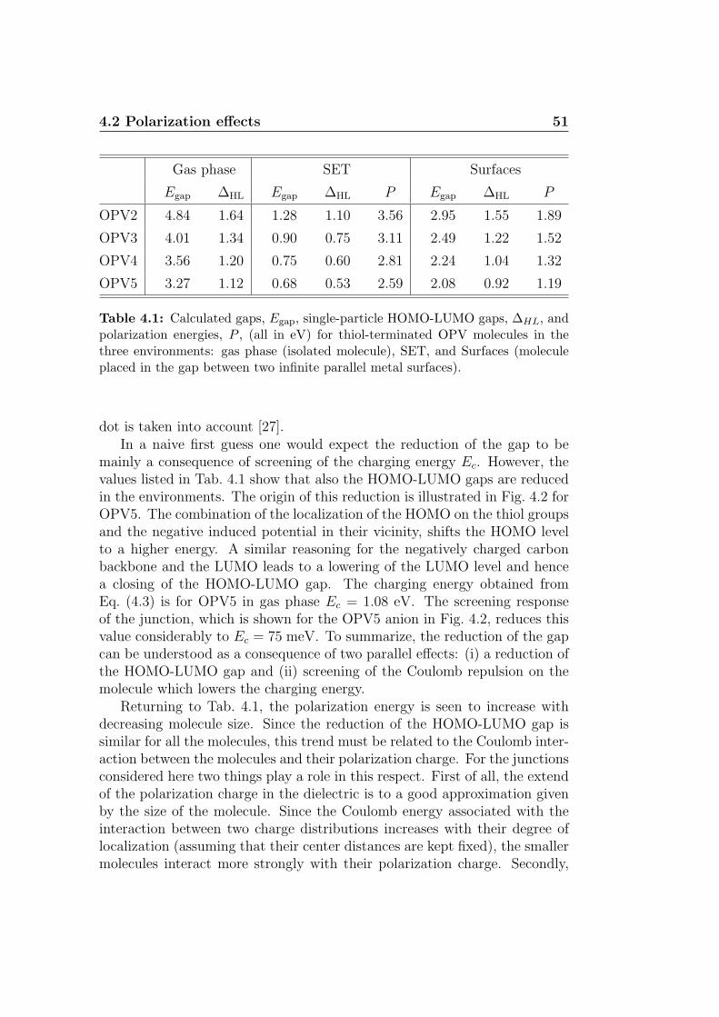
4.2 Polarization effects 51
Gas phase SET Surfaces
Egap ∆HL Egap ∆HL P Egap ∆HL P
OPV2 4.84 1.64 1.28 1.10 3.56 2.95 1.55 1.89
OPV3 4.01 1.34 0.90 0.75 3.11 2.49 1.22 1.52
OPV4 3.56 1.20 0.75 0.60 2.81 2.24 1.04 1.32
OPV5 3.27 1.12 0.68 0.53 2.59 2.08 0.92 1.19
Table 4.1: Calculated gaps, Egap, single-particle HOMO-LUMO gaps, ∆HL, andpolarization energies, P , (all in eV) for thiol-terminated OPV molecules in thethree environments: gas phase (isolated molecule), SET, and Surfaces (moleculeplaced in the gap between two infinite parallel metal surfaces).
dot is taken into account [27].In a naive first guess one would expect the reduction of the gap to be
mainly a consequence of screening of the charging energy Ec. However, thevalues listed in Tab. 4.1 show that also the HOMO-LUMO gaps are reducedin the environments. The origin of this reduction is illustrated in Fig. 4.2 forOPV5. The combination of the localization of the HOMO on the thiol groupsand the negative induced potential in their vicinity, shifts the HOMO levelto a higher energy. A similar reasoning for the negatively charged carbonbackbone and the LUMO leads to a lowering of the LUMO level and hencea closing of the HOMO-LUMO gap. The charging energy obtained fromEq. (4.3) is for OPV5 in gas phase Ec = 1.08 eV. The screening responseof the junction, which is shown for the OPV5 anion in Fig. 4.2, reduces thisvalue considerably to Ec = 75 meV. To summarize, the reduction of the gapcan be understood as a consequence of two parallel effects: (i) a reduction ofthe HOMO-LUMO gap and (ii) screening of the Coulomb repulsion on themolecule which lowers the charging energy.
Returning to Tab. 4.1, the polarization energy is seen to increase withdecreasing molecule size. Since the reduction of the HOMO-LUMO gap issimilar for all the molecules, this trend must be related to the Coulomb inter-action between the molecules and their polarization charge. For the junctionsconsidered here two things play a role in this respect. First of all, the extendof the polarization charge in the dielectric is to a good approximation givenby the size of the molecule. Since the Coulomb energy associated with theinteraction between two charge distributions increases with their degree oflocalization (assuming that their center distances are kept fixed), the smallermolecules interact more strongly with their polarization charge. Secondly,

52 Characterization of an OPV5 SET
with the electrode spacing given by the length of the molecules, the averagedistance between the polarization charge in the electrodes and the molecularcharge increases with decreasing molecule size. As above this results in ahigher Coulomb energy and hence also a larger polarization energy. Thelatter effect is clearly demonstrated by the last column in Tab. 4.1 wherethe dielectric is absent. The polarization energy for the shortest moleculeOPV2 is 0.7 eV larger than the one for OPV5. In the SET geometry thisdifference is 0.97 eV, indicating that the latter effect dominates the increaseof the polarization energy for the smaller molecules.
In the following the different contributions to the polarization energy ofOPV5 in the SET environment will be discussed. Due to its relatively highdielectric constant, the gate dielectric must be expected to have a large in-fluence on the polarization energy. For example, assuming that the gatedielectric is equivalent to an infinite dielectric surface, the image chargestrength is given by qεr = (εr − 1)/(εr + 1). For εr = 10 this results in animage charge strength of almost unity corresponding to metallic screeningproperties. The important role of the gate dielectric is clearly demonstratedby the large difference between the polarization energies for the SET andSurfaces environments in Tab. 4.1. For OPV5 the value for the latter of1.19 eV is less than half the value for the SET environment which is 2.59 eV.The reduction of the molecular gap in the OPV5 SET has thus equivalentcontributions from the source/drain electrodes and the gate dielectric. Note,however, that the contribution from the gate dielectric is highly dependent onits dielectric constant. With a dielectric constant of εr = 3.9 correspondingto SiO2 the polarization energy for OPV5 was reduced to 2.11 eV.
The contribution from the gate electrode was found to be negligible. Thereason for this is twofold. First, the dielectric screens the molecular charge.Therefore the net charge seen by the gate electrode is q − qεr and not thebare charge of the molecule. Second, due to the relatively large distancebetween the gate electrode and the molecule the Coulomb interaction withthe polarization charge in the gate is small. A simple image charge estimateshows that the thickness of the gate dielectric must be ∼ 1 nm in order to seea contribution of ∼ 0.1 eV to the polarization energy from the gate electrode.
4.3 Gate coupling
The gate electrode and its capacitive coupling to the molecule is fundamentalfor the functionality of single-molecule SETs. It allows to shift the molecularlevels by simple electrostatic means and thereby turn the current on and off.The following section addresses the gate coupling in the OPV5 SET and its
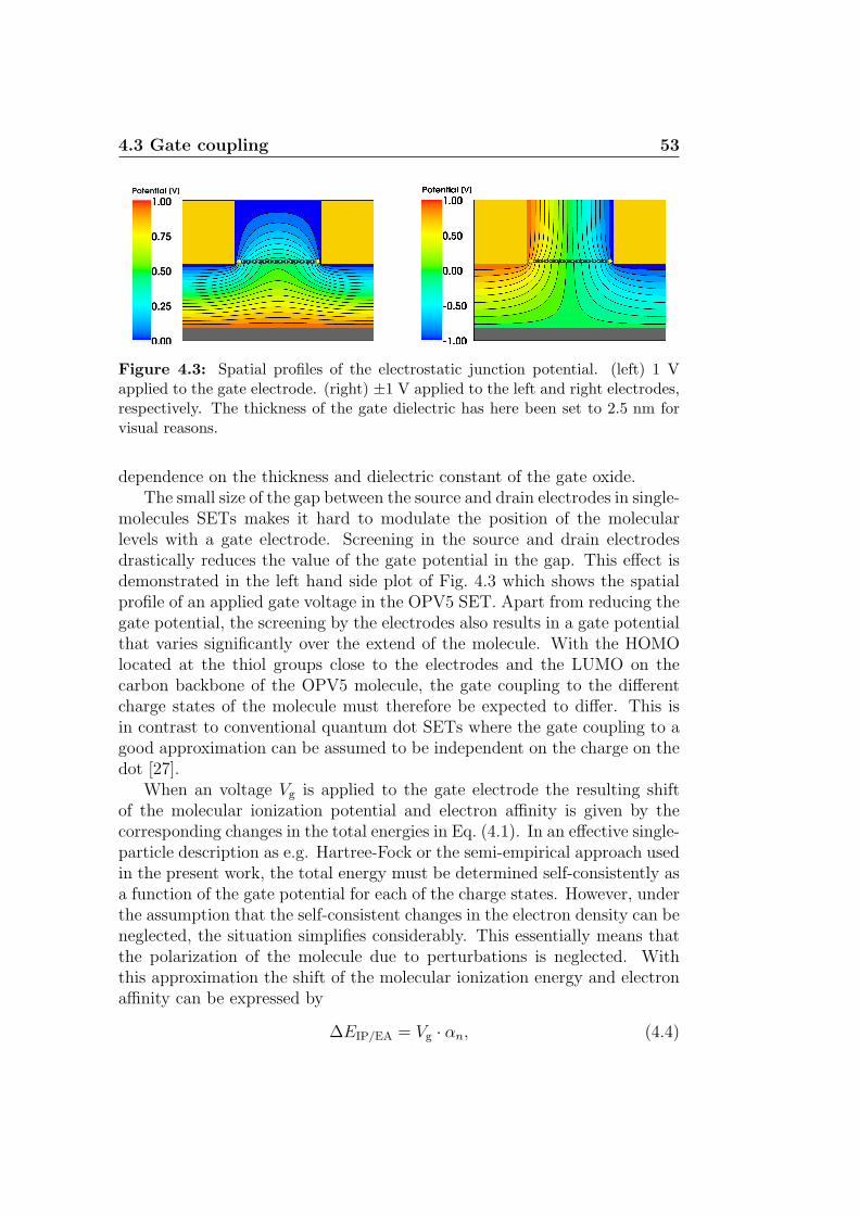
4.3 Gate coupling 53
Figure 4.3: Spatial profiles of the electrostatic junction potential. (left) 1 Vapplied to the gate electrode. (right) ±1 V applied to the left and right electrodes,respectively. The thickness of the gate dielectric has here been set to 2.5 nm forvisual reasons.
dependence on the thickness and dielectric constant of the gate oxide.The small size of the gap between the source and drain electrodes in single-
molecules SETs makes it hard to modulate the position of the molecularlevels with a gate electrode. Screening in the source and drain electrodesdrastically reduces the value of the gate potential in the gap. This effect isdemonstrated in the left hand side plot of Fig. 4.3 which shows the spatialprofile of an applied gate voltage in the OPV5 SET. Apart from reducing thegate potential, the screening by the electrodes also results in a gate potentialthat varies significantly over the extend of the molecule. With the HOMOlocated at the thiol groups close to the electrodes and the LUMO on thecarbon backbone of the OPV5 molecule, the gate coupling to the differentcharge states of the molecule must therefore be expected to differ. This isin contrast to conventional quantum dot SETs where the gate coupling to agood approximation can be assumed to be independent on the charge on thedot [27].
When an voltage Vg is applied to the gate electrode the resulting shiftof the molecular ionization potential and electron affinity is given by thecorresponding changes in the total energies in Eq. (4.1). In an effective single-particle description as e.g. Hartree-Fock or the semi-empirical approach usedin the present work, the total energy must be determined self-consistently asa function of the gate potential for each of the charge states. However, underthe assumption that the self-consistent changes in the electron density can beneglected, the situation simplifies considerably. This essentially means thatthe polarization of the molecule due to perturbations is neglected. Withthis approximation the shift of the molecular ionization energy and electronaffinity can be expressed by
∆EIP/EA = Vg · αn, (4.4)
54 Characterization of an OPV5 SET
where αn is the gate coupling to the molecular orbital n from which theelectron is added or removed. With the assumption above the gate couplingscan be obtain from the first order change ∆εi in the molecular single-particlelevels,
αn ≈ ∆εn = 〈n|αg(r)|n〉. (4.5)
Here αg is the characteristic potential that results from applying a unit volt-age to the gate electrode.
In the following the gate couplings to the HOMO and LUMO, and therebyalso the shift of the IP and EA with an applied gate voltage, are considered.Their dependence on the thickness and the dielectric constant of the gatedielectric is shown on the left and right plots of Fig. 4.4, respectively. Fur-thermore, the line denoted Mean shows the average of the gate couplings tothe atomic sites of the molecule.
As expected, the gate couplings to the HOMO and LUMO orbitals differmarkedly with the latter being approximately twice as large as the former.The mean gate coupling to the atomic sites of the molecules is close to theLUMO gate coupling. This can be attributed to the fact that the LUMO isdistributed more uniformly on the molecule as compared to the HOMO (seeFig. 4.1).
The left plot clearly shows the effect of using a thin dielectric layer. Asignificant increase in the gate coupling can be obtained by decreasing thelayer thickness to a few namometers. From a practical point of view this ishowever not as straight forward as it sounds since varying material propertiesand leakage currents to the gate electrode play an important role for ultrathinoxide layers [2].
Alternatively, a higher dielectric constant of the gate oxide can help toincrease the gate coupling. However, as the right plot shows, increasing thedielectric constant beyond ∼ 10 does not result in any significant increase ofthe gate coupling. The saturation of the gate coupling is due to screeningin the metallic source and drain electrodes. The same screening is respon-sible for a decreasing gate coupling when the molecule is elevated from thedielectric surface. This effect is illustrated by the spatial profile of the gatepotential in Fig. 4.3 which decreases rapidly as a function of the distance tothe gate dielectric.
Similar conclusions as the above have been drawn in a recent theoreticalstudy on gate coupling in nanoscale junctions [70]. This work also studiedthe effect of changing the geometry of the source and drain electrodes. Ajunction with tapered electrodes having a triangular shape was found to havea substantially greater gate coupling than the one with infinite electrodesconsidered in the present work. This, in particular, when the molecule was

4.4 Stability diagram 55
0 1 2 3 4 5 6 7
oxide thickness [nm]
0.0
0.2
0.4
0.6
0.8
1.0
gate
couplin
g
MeanHOMOLUMO
0 20 40 60 80 100εr
0.0
0.1
0.2
0.3
0.4
0.5
gate
couplin
g
MeanHOMOLUMO
Figure 4.4: Gate couplings αn to the HOMO and LUMO orbitals in the OPV5SET. The line denoted Mean is the average of the gate couplings on the atomicpositions of the OPV5 molecule. (left) Gate coupling as a function of gate oxidethickness with εr = 10. (right) Gate coupling as a function of the dielectricconstant εr with an oxide thickness of 5 nm.
elevated from the surface of the gate dielectric. The screening effect due to theelectrode geometry is therefore another significant parameter in determiningthe gate coupling of a nanoscale junction.
4.4 Stability diagram
The charge stability diagram for the OPV5 SET has been calculated byevaluating total energies of the neutral, singly charged and doubly chargedmolecule as a function of gate and source-drain voltage. The assumptionthat the molecule remains chemically stable in the considered charge statesis in agreement with experimental findings [20, 49]. The Fermi energy of themetallic source and drain electrodes is treated as a parameter and placedin the gap between the ionization potential and the electron affinity. Theresulting stability diagram is depicted in Fig. 4.5 where the colour indicatesthe number of levels that are located in the bias window. The source-drainbias has been applied symmetrically to the electrodes as illustrated in theright plot of Fig. 4.3 for Vsd = 2 V . It should be noted that the voltage dropacross the junction is non-linear close to the dielectric interface where themajority of the drop occurs close to the electrodes.
Like the experimentally observed stability diagram [20], the calculated di-agram is characterized by a big central diamond corresponding to the neutral

56 Characterization of an OPV5 SET
-3 -2 -1 0 1 2 3
Vg [V]
-0.4
-0.2
0.0
0.2
0.4
Vsd
[V
] N+1
UN
2α
2α HOMO
NN−1
LUMO
Vsd = 0.5 V
LUMO
HOMO
Figure 4.5: Stability diagram and molecular orbitals at finite bias. (left) Calcu-lated charge stability diagram for the OPV5-SET. The color indicates the numberof levels located inside the bias window (black: 0, red: 1, yellow: 2) (right) Molec-ular orbitals of the OPV5 molecule at Vsd = 0.5 V. The non-linear diamond edgeson the left site of the central diamond is a consequence of the localization of theHOMO at the right electrode.
state of the molecule surrounded by two small diamonds corresponding tothe positively and negatively charged molecule. Since only the ground statesof the neutral and charged molecule are considered, the stability diagramcontains no lines due to excited states of the molecule. This could e.g. be vi-brational excitations which have been observed experimentally with energiesranging from a few meV to ∼ 100 meV. A recent theoretical study has shownthat some of the vibrational excitations are expected to involve the goldatoms to which the molecule binds [67]. Electronic excitations of the OPV5molecule with electrons/holes occupying higher/lower molecular orbitals haveenergies on the order of the single-particle level spacings (∼ 100 meV). Theseare therefore harder to observe experimentally.
The addition energy given by the height of the central diamond is equalto the gap of the molecule under finite bias conditions. Compared to the zerobias gap of 0.68 eV from Tab. 4.1 a substantial decrease of the gap underfinite bias is found. From Fig. 4.5 a value of ∼ 0.50 eV is read off. The lowervalue of the addition energy stems from the non-linear edges on the left sideof the central diamond which indicates that the single-particle levels are biasindependent. Indeed, it was found that HOMO localizes at the negativelybiased electrode as illustrated in Fig. 4.5. As a consequence, the HOMO levelmoves upwards with the applied source-drain voltage making the state withonly one electron in the HOMO energetically favourable compared to the

4.5 Conclusion and outlook 57
neutral state which has a doubly occupied HOMO. The fact that the energyof the neutral molecule increases more than the energy of the cation as afunction of the source-drain bias, reduces the ionization energy and hencealso the threshold for pulling out an electron from the molecule. With asource-drain voltage of Vsd = 0.5 V corresponding to the top of the centraldiamond in Fig. 4.5, the shift of the HOMO level was ∼ 0.15 eV, in goodagreement with the discrepancy between the zero bias and finite bias gapsdiscussed above.
The height of the two smaller diamonds correspond to the addition ener-gies of the positively and negatively charged cation and anion, respectively.For these states the addition energy is given by the difference between the firstand second ionization potential/electron affinity. In terms of total energiesthis is
EN±1add = EN + EN±2 − 2EN±1. (4.6)
The small addition energies associated with these states is due to their halffilled frontier orbitals. Therefore, only the charging energy in Eq. (4.3) con-tributes when adding/removing an electron to/from the anion/cation. Theresulting charging energies are ∼ 50 meV and ∼ 85 meV, respectively. Thedifference in charging energies of the anion and cation is a consequence ofthe different spatial distributions of the HOMO and LUMO.
As expected from the considerations in the previous section the gate cou-plings to the ionization potential and electron affinity differ markedly. InFig. 4.5 these are given by the left and right slopes of the central diamondedges, respectively. Similar variations in the gate couplings have also beenobserved in a recent experiment [49]. The slopes of the diamond edges inFig. 4.5 agree well with the calculated gate couplings in Fig. 4.4, where weread off the values α
HOMO∼ 0.12 and α
LUMO∼ 0.25 for an oxide thickness
of 5 nm. This is also in good agreement with the value ∼ 0.2 reported ex-perimentally [20]. Often, the exact position of the molecule in experimentsis relatively unknown. However, the good agreement between the gate cou-plings suggests that the molecule also in the experiment is positioned directlyon the gate oxide.
4.5 Conclusion and outlook
In conclusion, the present chapter has demonstrated that polarization playsan important role in single-molecule SETs. For the junction consideredhere, a gap renormalization of ∼ 2.6 eV was found for the OPV5 molecule.The renormalization could be attributed to both a reduction of the HOMO-LUMO gap and a reduction of the Coulomb interaction. It should be noted

58 Characterization of an OPV5 SET
that the semi-empirical method applied in the present work, leaves someuncertainty on the calculated gap of 680 meV for OPV5 in the junction. Asmentioned, this is likely to be an underestimation. Nevertheless, the experi-mentally reported value of ∼ 300 meV is considerably lower than this. Differ-ent effects not considered in the present work can help to explain this discrep-ancy. For example, the formation of polarons upon charging of the moleculeis known to result in relaxation energies on the order of ∼ 200−300 meV forOPV-molecules [71]. Furthermore, a larger polarization energy is obtained ifthe molecule is positioned closer to the metallic electrodes where the screen-ing is more pronounced. Taking into account these additional effects, theobserved gap of ∼ 300 meV might not seem that unlikely after all.
In order to address the effect of junction polarization on electronic andspin excitations of the molecule, model Hamiltonians based on the effectivemany-body Hamiltonian in Eq. (2.20) must be developed. The Pariser-Parr-Pople Hamiltonian, which is considered in Chap. 6 in a different context(see Eq. 6.3), is an example of a simple model Hamiltonian description forconjugated molecules. Here, the Hamiltonian is expressed in a basis of pz
orbitals localized on each carbon atom in molecule. Taking into account thescreening of the Coulomb interaction in Eq. (2.20) leads to a renormalizationof the Coulomb matrix elements in the Pariser-Parr-Pople Hamiltonian and amodification of the onsite energies of the pz orbitals. Since an exact treatmentof the Pariser-Parr-Pople Hamiltonian is limited to models with relative fewbasis orbitals, models using the molecular orbitals of the molecular subunitsas basis orbitals have been developed [72]. The impact of junction screeningon the molecular excitations of such model Hamiltonians is subject for furtherstudies. With the inclusion of image charge effects at the level of the basisfunctions, it can be addressed to which extend the picture of image chargestabilized states in Ref. [49] is correct.

Chapter 5
Surface polarization and theGW approximation
Understanding the electronic structure of metal-molecule interfaces is a fun-damental challenge in molecule-based electronics. The electronic transportproperties of a metal-molecule interface are determined by the alignmentbetween the molecular levels and the Fermi energy of the metal substrate.Factors like hybridization with the metal substrate, dipole formation at theinterface as well as the polarization of the substrate in response to chargecarriers on the molecule play an important role in this respect [73]. It hasbeen demonstrated by several experiments that study the electronic structureof individual molecules, self-assembled monolayers and organic thin filmson metal surfaces using photoemission techniques and scanning tunnelingspectroscopy, that the molecular electronic structure is modified at the in-terface [16, 43, 74, 75].
Due to the hybridization with the metal substrate, first-principles studiesof the interface are based on an atomic description of both the moleculeand the metal. The electronic structure is most often obtained within theframework of density functional theory (DFT). In this context the eigenvaluesof the effective single-particle Kohn-Sham Hamiltonian are interpreted asexcitation energies. As DFT is a ground state theory this interpretation isquestionable. In particular, the intriguing many-body effects associated withthe polarization of the metal substrate and its effect on molecular levels arecompletely missing from DFT as well as other mean-field descriptions.
Recently, theoretical studies of single molecules physisorbed on metallicand dielectric surfaces have demonstrated that the Green’s function basedGW method captures the dynamical screening effects from the surface po-larization. As a consequence, the molecular gaps were reduced by severaleV [76, 77, 78]. Similar effects have been observed in GW calculations on
60 Surface polarization and the GW approximation
a simple model Hamiltonian for the interface [79]. Other GW studies ofpolarization effects at interfaces have demonstrated band-gap narrowing atmetal-semiconductor interfaces [80, 81] and state localization in metal em-bedded semiconductor nanorods [82]. Also, the GW approximation havebeen demonstrated to describe the internal polarization of bulk polymer ma-terials [83] and molecular self-assembled monolayers [84].
5.1 The GW approximation
The GW approximation originates from the so-called Hedin equations [85, 86]which form a closed set of equations for the many-body Green’s function.Despite being formally exact, the complexity of the self-consistent frame-work provided by Hedin’s equations necessitates the use of approximationsin practical calculations. The simplest approximation to Hedin’s equationsis the GW approximation which neglects the so-called vertex corrections tothe electronic self-energy.
In the GW approximation the electronic self-energy Σ is given by theproduct of the Green’s function G and the dynamically screened interactionW , and can be written symbolically as 1
Σ(1, 2) = iG(1, 2)W (1, 2), (5.1)
where the short-hand notation 1 = (r1, t1) has been introduced. The Green’sfunction obeys the usual Dyson equation
G(1, 2) = G0(1, 2) +
∫d3d4 G0(1, 3)Σ(3, 4)G(4, 2) (5.2)
with G0 denoting the Hartree Green’s function. The screened interaction Wis given by the Dyson-like equation
W (1, 2) = V (1, 2) +
∫d3d4 V (1, 3)Π(3, 4)W (4, 2), (5.3)
where V is the bare Coulomb interaction and
Π(1, 2) = −iG(1, 2)G(2, 1) (5.4)
1The equations given here are for the time ordered (zero temperature) Green’s function
G(1, 2) = −i〈T [ψ(1)ψ†(2)]〉.

5.1 The GW approximation 61
ΣGW == + + + . . .
Figure 5.1: Diagrammatic representation of the GW self-energy. The single anddouble wavy lines denotes the bare (V ) and the screened Coulomb interaction (W ),respectively. The polarization function Π is represented by the bubble diagrams.
is the polarization function in the random-phase approximation (RPA) whichcontains the response of the system to an added hole or electron. The di-agrammatic representation of the GW self-energy in Eq. (5.1) is illustratedin Fig. 5.1. It can be regarded as a generalization of the exchange potentialΣx = iGV in Hartree-Fock (represented by the first diagram in the secondequality) which does not take into account screening effects.
In fully self-consistent GW the set of coupled equations for Σ, G, Π, andW are solved iteratively until the Green’s function has converged. However,due to the computational requirement of a fully self-consistent GW scheme,first-principles GW calculations are usually carried out non-selfconsistently.This approach, which is referred to as G0W0, starts from an approximateG0 from which a single self-energy iteration is carried out to obtain thefinal Green’s function. In contrast to fully self-consistent GW, this has thedisadvantage that the final result depends on the starting Green’s function.
A self-consistent GW scheme has another advantage that it obeys themacroscopic conservation laws. For example, the conservation of particlenumber guaranteed by a self-consistent GW scheme means that the continu-ity equation
∂t1ρ(1) +∇1 · j(1) = 0 (5.5)
is satisfied when the electronic charge density ρ and the current density isobtained from the self-consistent Green’s function. This is due to Kadanoffand Baym [87, 88] who proved that an approximation for the self-energy Σ isconserving when it can be obtained as a functional derivative of a so-calledΦ-functional with respect to G
Σ(1, 2) =δΦ[G]
δG(1, 2). (5.6)
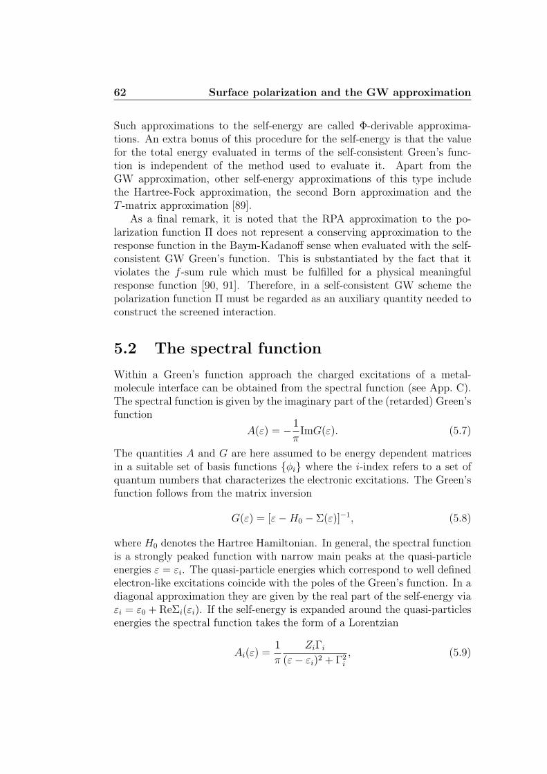
62 Surface polarization and the GW approximation
Such approximations to the self-energy are called Φ-derivable approxima-tions. An extra bonus of this procedure for the self-energy is that the valuefor the total energy evaluated in terms of the self-consistent Green’s func-tion is independent of the method used to evaluate it. Apart from theGW approximation, other self-energy approximations of this type includethe Hartree-Fock approximation, the second Born approximation and theT -matrix approximation [89].
As a final remark, it is noted that the RPA approximation to the po-larization function Π does not represent a conserving approximation to theresponse function in the Baym-Kadanoff sense when evaluated with the self-consistent GW Green’s function. This is substantiated by the fact that itviolates the f -sum rule which must be fulfilled for a physical meaningfulresponse function [90, 91]. Therefore, in a self-consistent GW scheme thepolarization function Π must be regarded as an auxiliary quantity needed toconstruct the screened interaction.
5.2 The spectral function
Within a Green’s function approach the charged excitations of a metal-molecule interface can be obtained from the spectral function (see App. C).The spectral function is given by the imaginary part of the (retarded) Green’sfunction
A(ε) = − 1
πImG(ε). (5.7)
The quantities A and G are here assumed to be energy dependent matricesin a suitable set of basis functions φi where the i-index refers to a set ofquantum numbers that characterizes the electronic excitations. The Green’sfunction follows from the matrix inversion
G(ε) = [ε−H0 − Σ(ε)]−1, (5.8)
where H0 denotes the Hartree Hamiltonian. In general, the spectral functionis a strongly peaked function with narrow main peaks at the quasi-particleenergies ε = εi. The quasi-particle energies which correspond to well definedelectron-like excitations coincide with the poles of the Green’s function. In adiagonal approximation they are given by the real part of the self-energy viaεi = ε0 + ReΣi(εi). If the self-energy is expanded around the quasi-particlesenergies the spectral function takes the form of a Lorentzian
Ai(ε) =1
π
ZiΓi
(ε− εi)2 + Γ2i
, (5.9)

5.2 The spectral function 63
where the width of the quasi-particle peak Γi = ZiImΣi(εi) corresponds tothe inverse lifetime of the quasi-particle and
Zi =
[1− ∂ReΣi
∂ε
∣∣∣∣ε=εi
]−1
≤ 1 (5.10)
is the spectral weight of the quasi-particle.
5.2.1 First-principles calculations
As mentioned in the introductory part of this chapter, first-principles calcu-lations are often based on DFT. For the Green’s function this amounts toapproximating the non-local and energy dependent self-energy Σ by the lo-cal and energy independent exchange-correlation potential Vxc. In real-spacenotation this is
Σ(r, r′, ε) = Vxc(r)δ(r− r′). (5.11)
The corresponding Kohn-Sham (KS) DFT Green’s function
GKS(ε) = [ε−H0 − Vxc]−1 (5.12)
has poles at the eigenvalues εKSi of the effective single-particle Kohn-Sham
Hamiltonian. From a pragmatic point of view this assigns the meaning of thequasi-particle energies to the Kohn-Sham eigenvalues. From the variationalderivation of DFT, there is, however, no reason why the Kohn-Sham eigen-values should correspond to excitation energies. In particular, the exchange-correlation potential is constructed to give the correct ground state energyand not excitation energies. The so-called bandgap problem of DFT, i.e. theempirical fact that DFT systematically underestimates bandgaps of solidsand molecules, is a consequence of this [92, 93].
In first-principles GW calculations, the quasi-particles energies are usuallyobtained in a perturbative manner from the eigenvalues of the Kohn-ShamHamiltonian in DFT [94]. Based on the assumption that the Kohn-Shameigenvalues εKS
i are good approximations to the quasi-particle energies, theGW quasi-particle energies can be obtained in first order perturbation theoryas
εi = εKSi + Zi∆Σi. (5.13)
Here ∆Σi = 〈φKSi |Σ(εKS
i ) − Vxc|φKSi 〉 is the matrix element of the difference
between the GW self-energy and the exchange-correlation potential from theDFT calculation evaluated with the eigenfunction φKS
i of the Kohn-ShamHamiltonian. This procedure for the calculation of the quasi-particle energiesis in the spirit of G0W0 approach with the self-energy calculated from theKohn-Sham Green’s function in Eq. (5.12).

64 Surface polarization and the GW approximation
5.3 Renormalization of molecular levels
The effect of surface polarization on molecular levels has recently been ad-dressed in a number of studies based on first-principles GW calculations ofmolecules physisorbed on various metallic and dielectric surfaces [76, 77, 78].With an atomic description of both the molecule and the surface these studiesaddress the polarization effects from the surface from a microscopic point ofview. This makes them complementary to the study of polarization effects insingle-molecule junction presented in the previous chapter which was basedon a macroscopic description of the junction.
For benzene physisorbed flat 3.25 A above a metallic graphite surface thegap of the molecule was found to be ∼ 3.2 eV smaller than the calculatedgas phase value [76]. Due to the weak hybridization between the molecularorbitals and the surface states this reduction of the molecular gap was as-cribed to the polarization of the surface. In contrast, the gap obtained fromKohn-Sham DFT eigenvalues did not show any change in the presence of thesurface environment.
Fig. 5.2 illustrates the Feynmans diagrams from the GW self-energy thatcontributes to the renormalization of the molecular levels. The infinite sumof diagrams with the polarization bubbles located in the surface and the baseline Green’s function on the molecule represents the interaction between anelectron added/removed to/from the molecule and the induced polarizationcharge of the surface. The response function given by the polarization bub-bles contains the full dynamical response of the surface. In general, dynam-ical effects are only important when the life-time of the excitations on themolecule is comparable to the response time of the surface. For the weaklycoupled benzene molecule this is not the case. Here, dynamical effects werefound to make a negligible contribution to the level renormalization. As aconsequence, the majority of the polarization induced shifts of the HOMOand LUMO levels of the benzene molecule could be accounted for by thestatic polarization integral
Pν =1
2
∫dr
∫dr′ φν(r)φ
∗ν(r
′)∆W (r, r′)φν(r′)φ∗ν(r), (5.14)
where φν is a molecular orbital of the isolated molecule and ∆W is the changein the screened interaction on the molecule due to the presence of the surface.The latter was approximated by the classical image potential from a metallicsurface, ∆W (r, r) = 1/2(z − z0), where z0 is the image plane position ofthe surface. The classical image potential has been shown to account for thestatic polarization response of a jellium surface [95]. For this metallic surfacethe image plane position was found to lie 0.5− 0.9 A outside the surface.
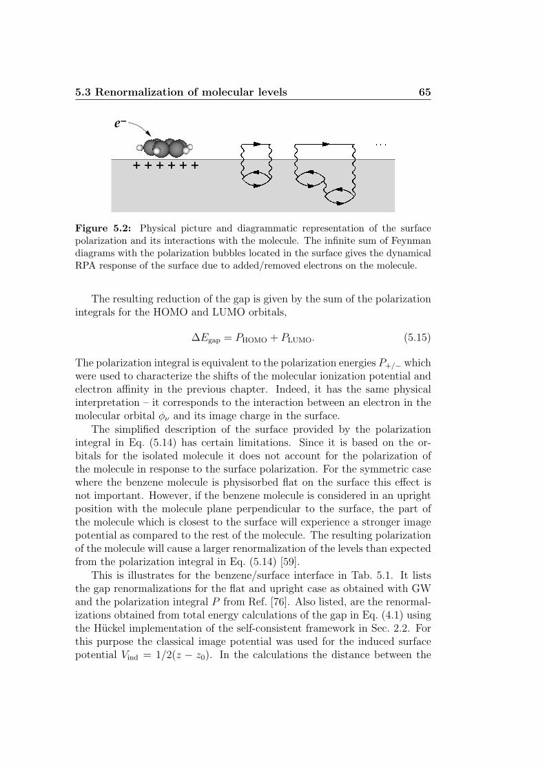
5.3 Renormalization of molecular levels 65
+ + + + + +
−e
Figure 5.2: Physical picture and diagrammatic representation of the surfacepolarization and its interactions with the molecule. The infinite sum of Feynmandiagrams with the polarization bubbles located in the surface gives the dynamicalRPA response of the surface due to added/removed electrons on the molecule.
The resulting reduction of the gap is given by the sum of the polarizationintegrals for the HOMO and LUMO orbitals,
∆Egap = PHOMO + PLUMO. (5.15)
The polarization integral is equivalent to the polarization energies P+/− whichwere used to characterize the shifts of the molecular ionization potential andelectron affinity in the previous chapter. Indeed, it has the same physicalinterpretation – it corresponds to the interaction between an electron in themolecular orbital φν and its image charge in the surface.
The simplified description of the surface provided by the polarizationintegral in Eq. (5.14) has certain limitations. Since it is based on the or-bitals for the isolated molecule it does not account for the polarization ofthe molecule in response to the surface polarization. For the symmetric casewhere the benzene molecule is physisorbed flat on the surface this effect isnot important. However, if the benzene molecule is considered in an uprightposition with the molecule plane perpendicular to the surface, the part ofthe molecule which is closest to the surface will experience a stronger imagepotential as compared to the rest of the molecule. The resulting polarizationof the molecule will cause a larger renormalization of the levels than expectedfrom the polarization integral in Eq. (5.14) [59].
This is illustrates for the benzene/surface interface in Tab. 5.1. It liststhe gap renormalizations for the flat and upright case as obtained with GWand the polarization integral P from Ref. [76]. Also listed, are the renormal-izations obtained from total energy calculations of the gap in Eq. (4.1) usingthe Huckel implementation of the self-consistent framework in Sec. 2.2. Forthis purpose the classical image potential was used for the induced surfacepotential Vind = 1/2(z − z0). In the calculations the distance between the

66 Surface polarization and the GW approximation
Position SC Huckel P GW
Flat 2.84 2.93 3.2
Upright 2.10 1.93 2.41
Table 5.1: Calculated reductions of the molecular gap Egap = EA−IP for benzeneon a metallic surface relative to its calculated gas phase value. The molecule isconsidered in a flat position and in an upright position on a metallic surface. Forthe two configurations the distance between the surface and the closest atom onthe molecule was 3.25 A and 2.21 A, respectively. The first column is the gapreductions obtained with the self-consistent method of Sec. 2.2. The second andthe third columns give the gap reductions resulting from the polarization integralP in Eq. (5.14) and GW calculations, respectively. Both of these have been takenfrom Ref. [76]. In the GW calculation the surface was described by an atomicgraphite surface. For the two other cases a simple image charge potential wasused to describe the polarization response of the surface. The position of theimage plane is z0 = 1 A from the outermost atomic layer of the surface. Forreference, the experimental gap phase gap for benzene is 10.42 eV.
molecule and the image plane of the surface was taken to be 2.25 A for theflat case and 1.21 A for the perpendicular case. This corresponds to an imageplane position z0 = 1 A outside the atomic surface plane in agreement withRef. [76].
For the flat case, the gap reductions from the total energy calculationsand the polarization integral are in good agreement. This is to be expectedsince both results are based on a classical image potential description of thesurface potential. The reduction obtained with GW is ∼ 0.3 eV larger. Abetter agreement is obtained if the image plane of the surface is placed atz0 = 1.25 A outside the atomic surface. This yields a reduction of 3.12 eVwith the self-consistent method. The gap is thus very sensitive to the distancebetween the molecule and the image plane implying that an accurate valuefor the latter is important. For atomic surfaces the image plane positionmust be determined in a separate calculation [68].
With the molecule is placed in an upright position on the surface the goodagreement between the gap reduction from the self-consistent method of thepresent work and the polarization integral is lost. In contrast to the flat case,the self-consistent method here gives the largest reductions of the gap. Thisis a consequence of the polarization of the molecule which is not accountedfor in the polarization integral P . In the self-consistent method the chargedistribution of the charged molecule relaxes towards the surface where the

5.3 Renormalization of molecular levels 67
potential due to the oppositely charged image charges is lower. This lowersthe total energy of the charged molecule, and in turn also the gap, morecompared to the case where the molecular charge distribution is not allowedto relax. Again, a better agreement with the GW result is obtained with theposition of the image plane equal to z0 = 1.25 A. This gives a gap reductionof 2.30 eV.
In the next chapter, the GW approximation is applied to study the molec-ular levels of isolated conjugated molecules described with a semi-empiricalmodel Hamiltonian. This study is intended to address the quality of the GWspectral function for isolated systems.

Chapter 6
Assessment of the GWapproximation for molecules
With the entry of nanoscience the use of the GW method for studyingelectronic structure has been extended to low-dimensional systems such asmolecules, fullerenes, carbon nanotubes, graphene [96, 97, 98, 99, 100, 101,102]. One strength of the GW method is that it accounts for the screening ofthe long range Coulomb interaction which is essential in finite systems. Themetal-molecule interface discussed in the previous chapter is a good exampleof this. Here, the finite extended of the molecular orbitals results in a surfacepolarization which in turn screens the Coulomb interaction on the moleculewhen an electron is added or removed from the molecule.
As the range of systems to which the GW approximation is being appliedcontinues to expand, critical investigations of the performance of GW forother systems than the crystalline solids become important. For example,with the application of GW to metal-molecule interfaces, knowledge on theperformance of GW on isolated molecules is of relevance. Different first-principles works have reported that the GW values for the ionization poten-tial and electron affinity of benzene are in good agreement with experimentalvalues [76, 101]. A more systematic study is, however, still missing.
So far, benchmark studies of the GW approximation have focused onHubbard models with local interactions [103, 104, 105, 106]. The generalconclusion from these works is that the GW approximation works well forsmall interaction strengths but fails for larger interactions strength. Theuse of GW in systems with local interactions is in fact unfortunate becausethe importance of electronic screening, which is the main effect described byGW, is weak in comparison to correlation effects.
In the following chapter benchmark GW calculations for π-conjugatedmolecules based on the semi-empirical Pariser-Parr-Pople (PPP) model [107,
70 Assessment of the GW approximation for molecules
108, 109] are presented. By comparing with exact results a direct and unbi-ased estimate of the quality of the GW approximation in molecular systemsis obtained.
6.1 Quasi-particle energies
The excitation spectrum of a system is contained in the spectral functionwhich has the following Lehmann representation (see App. C)
Ai(ε) =∑
n
[|〈ΨN+1
n |c†i |ΨN0 〉|2δ(ε− εn) + |〈ΨN−1
n |ci |ΨN0 〉|2δ(ε− εn)
]. (6.1)
The peaks of the spectral function are positioned at the quasi-particle en-ergies εn = EN+1
n − EN0 and εn = EN
0 − EN−1n corresponding to electronic
addition and removal energies, respectively. Here ENn denotes the total en-
ergy of the N -electron excited state |ΨNn 〉 with N referring to the neutral
state of the system. For molecules the first addition and the first removalenergy, i.e. n = 0, corresponds to the electron affinity and the ionizationpotential. In Hartree-Fock theory Koopman’s theorem [63] states that theseare equal to the energies of the highest occupied orbital (HOMO) and lowestunoccupied molecular orbital (LUMO) of the Hartree-Fock Hamiltonian. Inthe remaining of this chapter the HOMO and LUMO abbreviations will beused to refer to the ionization potential and electron affinity also outsideHartree-Fock theory. When the ionization potential and electron affinityare obtained from Koopman’s theorem, two important effects are neglected.One is the relaxation of the molecular orbitals when an electron is removedfrom or added to the molecule. The other is the correlation energy whichby definition is omitted in Hartree-Fock theory. With the generalizationof Koopman’s theorem to excited states it is instructive to write the exactquasi-particle energies as the sum of the three contributions
εn = εHFn + ∆relax + ∆corr, (6.2)
where εHFn denotes the n’th eigenvalue of the single-particle Hartree-Fock
Hamiltonian. The relaxation contribution is the correction that followsby calculating the quasi-particle energy from self-consistently determinedHartree-Fock energies of the neutral and the charged states N ± 1. Thelast term ∆corr is the remaining contribution from the correlation energy.
In extended systems the potential due to a single delocalized electron/holedecreases with the size of the system. Hence, in such systems there will be noor little relaxation of the states due to the addition/removal of an electron,
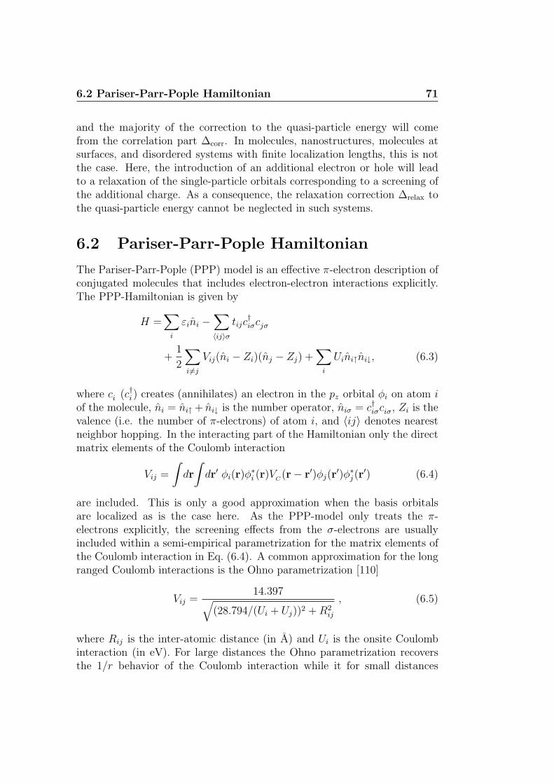
6.2 Pariser-Parr-Pople Hamiltonian 71
and the majority of the correction to the quasi-particle energy will comefrom the correlation part ∆corr. In molecules, nanostructures, molecules atsurfaces, and disordered systems with finite localization lengths, this is notthe case. Here, the introduction of an additional electron or hole will leadto a relaxation of the single-particle orbitals corresponding to a screening ofthe additional charge. As a consequence, the relaxation correction ∆relax tothe quasi-particle energy cannot be neglected in such systems.
6.2 Pariser-Parr-Pople Hamiltonian
The Pariser-Parr-Pople (PPP) model is an effective π-electron description ofconjugated molecules that includes electron-electron interactions explicitly.The PPP-Hamiltonian is given by
H =∑
i
εini −∑〈ij〉σ
tijc†iσcjσ
+1
2
∑i6=j
Vij(ni − Zi)(nj − Zj) +∑
i
Uini↑ni↓, (6.3)
where ci (c†i ) creates (annihilates) an electron in the pz orbital φi on atom iof the molecule, ni = ni↑ + ni↓ is the number operator, niσ = c†iσciσ, Zi is thevalence (i.e. the number of π-electrons) of atom i, and 〈ij〉 denotes nearestneighbor hopping. In the interacting part of the Hamiltonian only the directmatrix elements of the Coulomb interaction
Vij =
∫dr
∫dr′ φi(r)φ
∗i (r)VC
(r− r′)φj(r′)φ∗j(r
′) (6.4)
are included. This is only a good approximation when the basis orbitalsare localized as is the case here. As the PPP-model only treats the π-electrons explicitly, the screening effects from the σ-electrons are usuallyincluded within a semi-empirical parametrization for the matrix elements ofthe Coulomb interaction in Eq. (6.4). A common approximation for the longranged Coulomb interactions is the Ohno parametrization [110]
Vij =14.397√
(28.794/(Ui + Uj))2 +R2ij
, (6.5)
where Rij is the inter-atomic distance (in A) and Ui is the onsite Coulombinteraction (in eV). For large distances the Ohno parametrization recoversthe 1/r behavior of the Coulomb interaction while it for small distances
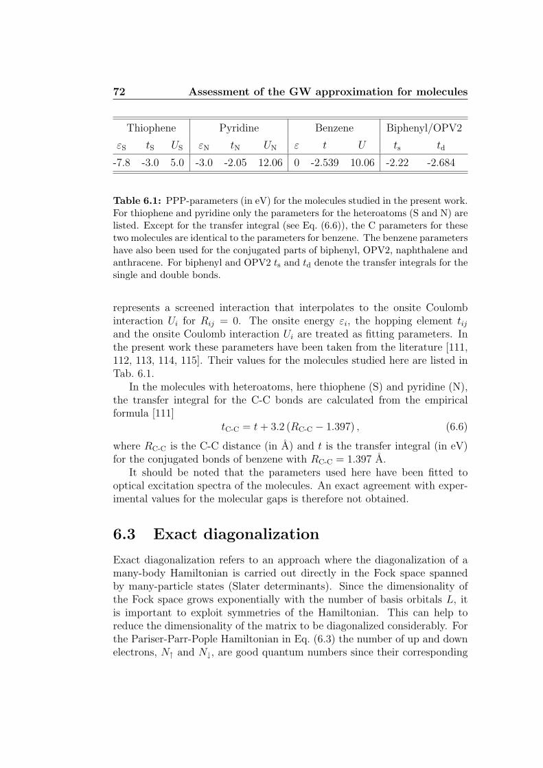
72 Assessment of the GW approximation for molecules
Thiophene Pyridine Benzene Biphenyl/OPV2
εS tS US εN tN UN ε t U ts td
-7.8 -3.0 5.0 -3.0 -2.05 12.06 0 -2.539 10.06 -2.22 -2.684
Table 6.1: PPP-parameters (in eV) for the molecules studied in the present work.For thiophene and pyridine only the parameters for the heteroatoms (S and N) arelisted. Except for the transfer integral (see Eq. (6.6)), the C parameters for thesetwo molecules are identical to the parameters for benzene. The benzene parametershave also been used for the conjugated parts of biphenyl, OPV2, naphthalene andanthracene. For biphenyl and OPV2 ts and td denote the transfer integrals for thesingle and double bonds.
represents a screened interaction that interpolates to the onsite Coulombinteraction Ui for Rij = 0. The onsite energy εi, the hopping element tijand the onsite Coulomb interaction Ui are treated as fitting parameters. Inthe present work these parameters have been taken from the literature [111,112, 113, 114, 115]. Their values for the molecules studied here are listed inTab. 6.1.
In the molecules with heteroatoms, here thiophene (S) and pyridine (N),the transfer integral for the C-C bonds are calculated from the empiricalformula [111]
tC-C = t+ 3.2 (RC-C − 1.397) , (6.6)
where RC-C is the C-C distance (in A) and t is the transfer integral (in eV)for the conjugated bonds of benzene with RC-C = 1.397 A.
It should be noted that the parameters used here have been fitted tooptical excitation spectra of the molecules. An exact agreement with exper-imental values for the molecular gaps is therefore not obtained.
6.3 Exact diagonalization
Exact diagonalization refers to an approach where the diagonalization of amany-body Hamiltonian is carried out directly in the Fock space spannedby many-particle states (Slater determinants). Since the dimensionality ofthe Fock space grows exponentially with the number of basis orbitals L, itis important to exploit symmetries of the Hamiltonian. This can help toreduce the dimensionality of the matrix to be diagonalized considerably. Forthe Pariser-Parr-Pople Hamiltonian in Eq. (6.3) the number of up and downelectrons, N↑ and N↓, are good quantum numbers since their corresponding

6.3 Exact diagonalization 73
L dimension memory
2 4 32 B
6 400 3 kB
8 4900 38 kB
10 63504 0.5 MB
12 853776 6.5 MB
14 11778624 90 MB
16 165636900 1.2 GB
Table 6.2: Dimensionality and memory requirements for a state vector of thehalf-filled subblock of the Fock space for different values of the number of basisorbitals L. The state vector is assumed stored in double floating point precision.
operators commute with the Hamiltonian. This implies that the diagonaliza-tion can be carried out in each of the (N↑, N↓)-subblocks of the Fock spaceindependently. The dimensionality d of each (N↑, N↓)-subblock is given bythe number of ways N↑ spin up electrons and N↓ spin down electrons can bedistributed over L basis orbitals,
d(N↑, N↓) =L!
N↑!(L−N↑)!× L!
N↓!(L−N↓)!. (6.7)
Most often the ground state is located in the half-filled subblock, i.e.N↑ = N↓ = L/2. The dimensionality of this subblock together with thememory requirements for a single state vector belonging to this subblock arelisted in Tab. 6.2 for different values of L. Already at L = 16 the memoryrequirements for a single state vector is on the order of the amount of RAMmemory available in modern computers. With such memory requirements afull diagonalization of the Hamiltonian is of course out of reach. However, ifonly the ground state and a few low lying excited states are needed, iterativemethods can be employed. Even with iterative methods one is restricted toa relatively small number of basis orbitals. To put things in perspective, thecurrent world record in exact diagonalization using iterative methods is a 22site Hubbard model with 9 and 8 up and down electrons. This corresponds toa Hilbert space dimension of ∼ 159 billion resulting in a memory requirementof ∼ 1 TB per state vector [116].
The following sections give a brief overview of some of the technical as-pects and algorithms of an exact diagonalization scheme. Apart from aniterative diagonalization method, a scheme for the calculation of the Green’sfunction is also presented.
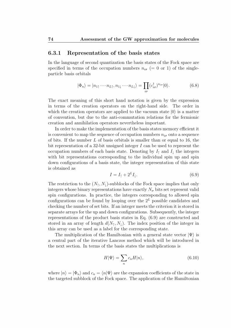
74 Assessment of the GW approximation for molecules
6.3.1 Representation of the basis states
In the language of second quantization the basis states of the Fock space arespecified in terms of the occupation numbers niσ (= 0 or 1) of the single-particle basis orbitals
|Φn〉 = |n1↑ · · ·nL↑, n1↓ · · ·nL↓〉 =∏iσ
(c†iσ)niσ |0〉. (6.8)
The exact meaning of this short hand notation is given by the expressionin terms of the creation operators on the right-hand side. The order inwhich the creation operators are applied to the vacuum state |0〉 is a matterof convention, but due to the anti-commutation relations for the fermioniccreation and annihilation operators nevertheless important.
In order to make the implementation of the basis states memory efficient itis convenient to map the sequence of occupation numbers niσ onto a sequenceof bits. If the number L of basis orbitals is smaller than or equal to 16, thebit representation of a 32-bit unsigned integer I can be used to represent theoccupation numbers of each basis state. Denoting by I↑ and I↓ the integerswith bit representations corresponding to the individual spin up and spindown configurations of a basis state, the integer representation of this stateis obtained as
I = I↑ + 2LI↓. (6.9)
The restriction to the (N↑, N↓)-subblocks of the Fock space implies that onlyintegers whose binary representations have exactly Nσ bits set represent validspin configurations. In practice, the integers corresponding to allowed spinconfigurations can be found by looping over the 2L possible candidates andchecking the number of set bits. If an integer meets the criterion it is stored inseparate arrays for the up and down configurations. Subsequently, the integerrepresentations of the product basis states in Eq. (6.9) are constructed andstored in an array of length d(N↑, N↓). The index position of the integer inthis array can be used as a label for the corresponding state.
The multiplication of the Hamiltonian with a general state vector |Ψ〉 isa central part of the iterative Lanczos method which will be introduced inthe next section. In terms of the basis states the multiplications is
H|Ψ〉 =∑
n
cnH|n〉, (6.10)
where |n〉 = |Φn〉 and cn = 〈n|Ψ〉 are the expansion coefficients of the state inthe targeted subblock of the Fock space. The application of the Hamiltonian

6.3 Exact diagonalization 75
Figure 6.1: 400×400 matrix representation of the PPP-Hamiltonian for benzenein the half-filled subblock of the Fock space with N↑ = N↓ = 3.
to a basis state |n〉 can be carried out using bitwise operations on the binaryrepresentation of the corresponding integer. This generates a new vector
H|n〉 =∑n′
〈n′|H|n〉|n′〉, (6.11)
where the number of nonzero terms depends on the sparsity of the Hamil-tonian. For states |n′〉 where the matrix element 〈n′|H|n〉 is different fromzero, the integer representation of the state must be mapped back to itsindex in the subblock basis in order to update the coefficients of the productstate H|Ψ〉. If the basis states are stored in increasing order of their integervalue, a binary search of the basis array can be used to find the index of agiven state in the basis. With this approach the memory requirements ofan additional look-up table that tabulates the correspondence between theinteger representation and the index is avoided.
In the Pariser-Parr-Pople Hamiltonian in Eq. (6.3) only the hopping termsgive rise to off-diagonal elements. The Coulomb interaction only reads offthe occupations numbers without modifying the basis states and is thereforediagonal. The inclusion of only nearest neighbor hopping results in highlysparse matrix representations. This is illustrated in Fig. 6.1 for the Hamil-tonian of benzene (L = 6) in the half-filled subspace. Due to the long rangeCoulomb interaction included in the PPP-Hamiltonian, all the diagonal ele-ments are of the same order of magnitude. This is in contrast to HubbardHamiltonians which only includes the onsite part of the Coulomb interaction

76 Assessment of the GW approximation for molecules
in Eq. (6.3). In this case the diagonal is dominated by states with doublyoccupied sites which results in eigenstates that are qualitative different fromthose of the PPP-Hamiltonian.
6.3.2 Calculating the ground state - Lanczos algorithm
The basic idea of iterative methods is to project the Hamiltonian onto theKrylov subspace K generated by repeated applications of H on an arbitraryinitial state |φ0〉, i.e.
K = span|φ0〉, H|φ0〉, H2|φ0〉, · · · , HM−1|φ0〉. (6.12)
In the Krylov subspace the extreme eigenvalues of the Hamiltonian convergefast with respect to the size M of the subspace, thus reducing the full diago-nalization to a manageable diagonalization of a M ×M matrix with M d.
In the Lanczos algorithm 1 the Hamiltonian is projected onto a speciallyconstructed orthogonalised Krylov basis in which the Hamiltonian has a tridi-agonal representation [118]. The basis vectors are generated recursively as
|φn+1〉 = H|φn〉 − an|φn〉 − b2n|φn−1〉, (6.13)
where the coefficient are given by
an =〈φn|H|φn〉〈φn|φn〉
and b2n =〈φn|φn〉
〈φn−1|φn−1〉(6.14)
with initial conditions b0 = 0 and |φ−1〉 = 0. At any point during the Lanczositerations only three Lanczos vectors need to be kept in memory, which makesthe algorithm memory efficient. In the basis of the normalized vectors (thebasis vectors above are not normalized) the Hamiltonian has the followingtridiagonal representation
H =
a0 b1 0 · · · 0
b1 a1 b2...
0 b2 a2. . . 0
.... . . . . . bM
0 · · · 0 bM aM
(6.15)
which can be readily diagonalized with methods for tridiagonal matricesyielding the ground state energy E0. In practice the Lanczos iterations are
1The present work has used the implementation from the IETL project [117].
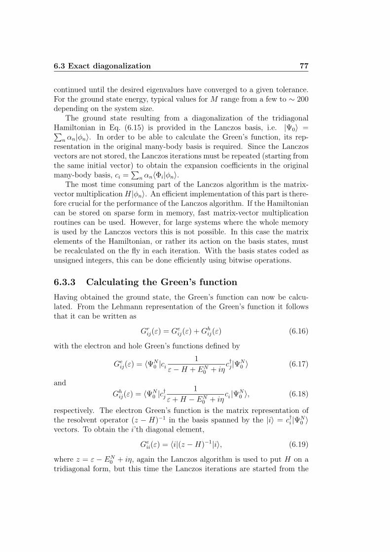
6.3 Exact diagonalization 77
continued until the desired eigenvalues have converged to a given tolerance.For the ground state energy, typical values for M range from a few to ∼ 200depending on the system size.
The ground state resulting from a diagonalization of the tridiagonalHamiltonian in Eq. (6.15) is provided in the Lanczos basis, i.e. |Ψ0〉 =∑
n αn|φn〉. In order to be able to calculate the Green’s function, its rep-resentation in the original many-body basis is required. Since the Lanczosvectors are not stored, the Lanczos iterations must be repeated (starting fromthe same initial vector) to obtain the expansion coefficients in the originalmany-body basis, ci =
∑n αn〈Φi|φn〉.
The most time consuming part of the Lanczos algorithm is the matrix-vector multiplicationH|φn〉. An efficient implementation of this part is there-fore crucial for the performance of the Lanczos algorithm. If the Hamiltoniancan be stored on sparse form in memory, fast matrix-vector multiplicationroutines can be used. However, for large systems where the whole memoryis used by the Lanczos vectors this is not possible. In this case the matrixelements of the Hamiltonian, or rather its action on the basis states, mustbe recalculated on the fly in each iteration. With the basis states coded asunsigned integers, this can be done efficiently using bitwise operations.
6.3.3 Calculating the Green’s function
Having obtained the ground state, the Green’s function can now be calcu-lated. From the Lehmann representation of the Green’s function it followsthat it can be written as
Grij(ε) = Ge
ij(ε) +Ghij(ε) (6.16)
with the electron and hole Green’s functions defined by
Geij(ε) = 〈ΨN
0 |ci1
ε−H + EN0 + iη
c†j|ΨN0 〉 (6.17)
and
Ghij(ε) = 〈ΨN
0 |c†j
1
ε+H − EN0 + iη
ci |ΨN0 〉, (6.18)
respectively. The electron Green’s function is the matrix representation ofthe resolvent operator (z − H)−1 in the basis spanned by the |i〉 = c†i |ΨN
0 〉vectors. To obtain the i’th diagonal element,
Geii(ε) = 〈i|(z −H)−1|i〉, (6.19)
where z = ε − EN0 + iη, again the Lanczos algorithm is used to put H on a
tridiagonal form, but this time the Lanczos iterations are started from the

78 Assessment of the GW approximation for molecules
normalized initial state |φ0〉 = |i〉/b0 where b20 = 〈i|i〉. In the generatedKrylov subspace the diagonal element of the Green’s function corresponds tothe matrix element b20[(ε−H +EN
0 + iη)−1]11, which can be obtained as thecontinued fraction [119]
Geii(ε) =
b20
z − a0 −b21
z − a1 −b22
z − a2 − · · ·
. (6.20)
Again the Lanczos iterations are continued until the frequency dependentGreen’s function element has converged. The elements of the hole Green’sfunction can be calculated similarly by starting the Lanczos iterations fromthe vector |i〉 = ci |ΨN
0 〉.
6.3.4 Correlation measure - von Neumann entropy
The following section demonstrates how a quantitative measure of the levelof correlations in a system can be obtained by considering the von Neumannentropy of the single-particle density matrix ρ. The entropy is defined by
S = −Tr[ρ log ρ] = −∑
n
ρn log ρn, (6.21)
where in the last equality ρ has been expressed in its diagonal representation,ρ =
∑n ρn|n〉〈n|.
In the basis of the atomic pz orbitals of the PPP-Hamiltonian the matrixelements of the reduced density matrix of the ground state |Ψ0〉 are given by(with the spin index suppressed)
ρij = 〈Ψ0|c†jci |Ψ0〉. (6.22)
The diagonal elements ρii of the density matrix correspond to the site oc-cupations ni of the ground state |Ψ0〉. When expressed in its diagonal rep-resentation ρn represents the occupation of the eigenstate |n〉 of the densitymatrix.
In the half-filled subblock of the Fock space the ground state entropyis limited to 0 ≤ S ≤ L log 2, where 2L is the dimension of the single-particle Hilbert space including spin. Here, S = 0 corresponds to a statewith no correlations, while the maximum value Smax = L log 2 for the entropycorresponds to a maximally correlated state. This follows from the naturaldiagonal representation of the density matrix in the two extreme cases (see

6.4 Results 79
below). Therefore, the number 0 ≤ S/Smax ≤ 1 represents a natural measureof the degree of correlation in the state |Ψ0〉.
By definition, Hartree-Fock theory is exact if the ground state in uncor-related. Hence, the ground state is given by the Slater determinant
|Ψ0〉 =∏νσ
c†νσ|0〉, (6.23)
where c†νσ are the creation operators for the single-particle Hartree-Fock or-bitals φν . Due to the mutual orthogonality of the HF orbitals, the densitymatrix is diagonal in this basis with eigenvalues equal to one for the occupiedand zero for the unoccupied (virtual) orbitals. As a consequence, S = 0 foran uncorrelated state as stated above.
Hubbard models where only onsite interactions are included give rise tostrongly correlated states. The singlet ground state |Ψs〉 of the two-siteHubbard model in the limit U t is an example of a maximally correlatedstate. Due to the high U/t-ratio, the energy cost of having two electronsat the same site becomes prohibitly high. The ground state is thereforecompletely dominated by the two states with singly occupied sites
|Ψs〉 =1√2
(c†2↑c
†1↓|0〉 − c†2↓c
†1↑|0〉
), (6.24)
where the positions of the spins refer to the site index. The correspondingdensity matrix is diagonal in the site basis with site occupations niσ = 1/2from which S = Smax follows. In general, maximally correlated states havedominating weight on small subsets of orthogonal determinants correspond-ing to the energetically most favorable basis states. In Hubbard models wherethe onsite Coulomb repulsion dominates over the kinetic energy these are thebasis states with no doubly occupied sites.
6.4 Results
The following two sections present the benchmark results for the seven con-jugated molecules in Tab. 6.3. In the first section the accuracy of the GWground state energies for the neutral molecules is represented in terms of thecorrelation energy. The second section focus on the spectral properties andthe different contributions from Eq. 6.2 to the quasi-particle energies in GW.The GW results reported here have been obtained with a fully self-consistentGW scheme without any further approximations to the electronic self-energyapart from the GW approximation itself (see Ref. [120] for details).
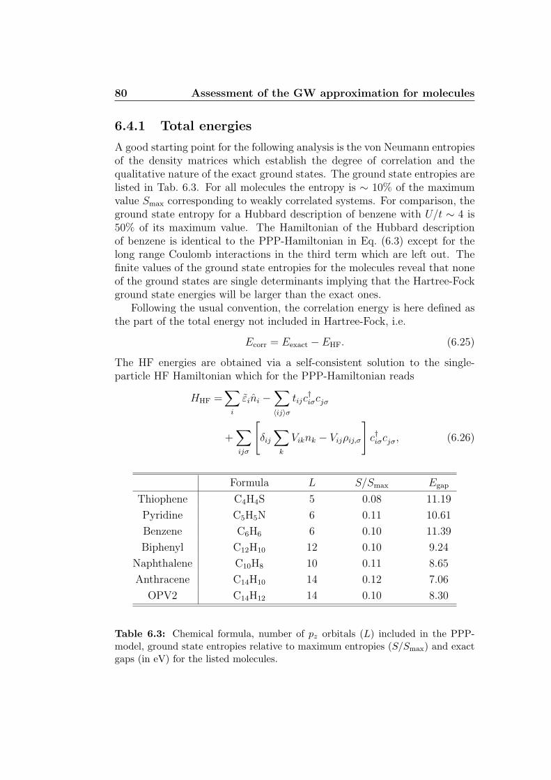
80 Assessment of the GW approximation for molecules
6.4.1 Total energies
A good starting point for the following analysis is the von Neumann entropiesof the density matrices which establish the degree of correlation and thequalitative nature of the exact ground states. The ground state entropies arelisted in Tab. 6.3. For all molecules the entropy is ∼ 10% of the maximumvalue Smax corresponding to weakly correlated systems. For comparison, theground state entropy for a Hubbard description of benzene with U/t ∼ 4 is50% of its maximum value. The Hamiltonian of the Hubbard descriptionof benzene is identical to the PPP-Hamiltonian in Eq. (6.3) except for thelong range Coulomb interactions in the third term which are left out. Thefinite values of the ground state entropies for the molecules reveal that noneof the ground states are single determinants implying that the Hartree-Fockground state energies will be larger than the exact ones.
Following the usual convention, the correlation energy is here defined asthe part of the total energy not included in Hartree-Fock, i.e.
Ecorr = Eexact − EHF. (6.25)
The HF energies are obtained via a self-consistent solution to the single-particle HF Hamiltonian which for the PPP-Hamiltonian reads
HHF =∑
i
εini −∑〈ij〉σ
tijc†iσcjσ
+∑ijσ
[δij∑
k
Viknk − Vijρij,σ
]c†iσcjσ, (6.26)
Formula L S/Smax Egap
Thiophene C4H4S 5 0.08 11.19
Pyridine C5H5N 6 0.11 10.61
Benzene C6H6 6 0.10 11.39
Biphenyl C12H10 12 0.10 9.24
Naphthalene C10H8 10 0.11 8.65
Anthracene C14H10 14 0.12 7.06
OPV2 C14H12 14 0.10 8.30
Table 6.3: Chemical formula, number of pz orbitals (L) included in the PPP-model, ground state entropies relative to maximum entropies (S/Smax) and exactgaps (in eV) for the listed molecules.

6.4 Results 81
Thiophene
Pyridine
Benzene
Biphenyl
Naphthalene
Anthracene
OPV2-1.6
-1.4
-1.2
-1.0
-0.8
-0.6
-0.4
-0.2
0.0
Eco
rr (
eV
)ExactGW
Figure 6.2: Exact and GW correlation energies of the neutral ground states forthe seven molecules. Both are calculated as the difference in total energy withrespect to the Hartree-Fock energy, i.e. Ecorr = E − EHF.
where εi = εi−∑
k 6=i VikZk and Vii = Ui. The last term contains the Hartreepotential which is diagonal in the site indices and the exchange potentialwhich has off-diagonal contributions. The resulting eigenfunctions φν are thecanonical molecular orbitals from which the ground state Slater determinantin Eq. (6.23) is constructed. The total energy EHF then follows by taking theexpectation value of the PPP-Hamiltonian with respect to the ground stateSlater determinant. The expectation value of the non-interacting part can beexpressed directly in terms of the reduced density matrix. For the interactingpart of the PPP-Hamiltonian, the expectation value can be evaluated by ap-plying Wick’s theorem to the product of creation and annihilation operatorshidden in the site occupation operator ni. The resulting expression for thetotal energy can be written as
EHF = 〈H〉HF =∑iσ
εiρii,σ −∑ijσ
tijρijσ
+1
2
∑ij
σσ′
Vij [ρii,σρjj,σ′ − δσ,σ′ρij,σρji,σ] . (6.27)
The second term in the last sum is the exchange energy whose diagonalcontribution removes the self-interactions included in the first Hartree term.

82 Assessment of the GW approximation for molecules
The GW total energy is identical to the HF energy above with the excep-tion that the exchange-correlation energy [121]
Exc =1
2i
∫Tr [Σr(ε)G<(ε) + Σ<(ε)Ga(ε)] dε (6.28)
replaces the exchange energy in HF and the GW density matrix obtainedfrom the GW Green’s function (see App. C) replaces the HF density matrix.
Fig. 6.2 shows the exact correlation energies of the neutral ground statestogether with those obtained from the GW approximation. For the series ofmolecules considered here the correlation energy constitute less than 0.5%of the total energies. Furthermore, as expected, it increases (in absolutesize) with the number of atoms in the molecule. The GW approximationperforms reasonably well for all the molecules capturing on average 66% ofthe correlation energy.
6.4.2 Spectral properties
For isolated systems such as molecules, true quasi-particles resembling single-particle excitations are characterized by having a weight close to unity (fornon-degenerate levels) in the spectral function, i.e.
Zn =∑
i
|〈ΨN+1n |c†i |ΨN
0 〉|2 ∼ 1. (6.29)
This is equivalent to the existence of a molecular orbital φν which allow theexcited state |ΨN+1
n 〉 to be written as the single-particle excitation c†ν |ΨN0 〉.
Fig. 6.3 shows the single-particle density of states (DOS),
D(ε) =∑
i
Ai(ε) (6.30)
for the OPV2 molecule on a logarithmic scale. The height of the peaks reflectsthe value of Zn (modulo degeneracies). The HF and, in particular, the GWapproximation reproduce the lowest lying excitations quite well while higherexcitations are poorly described. All the peaks in the HF spectrum have Zn =1 while GW shifts some spectral weight from the main peaks to tiny satellitestructures (at higher energies than shown on the plot). This is in agreementwith the exact results. For example, the exact spectral weight of the LUMOis ZLUMO ∼ 0.92 and ∼ 0.97 in GW. However, the GW satellites do notcorrespond to features in the exact spectrum. This shows that excitationswith Zn 1, i.e. excitations which do not have single-particle character, are
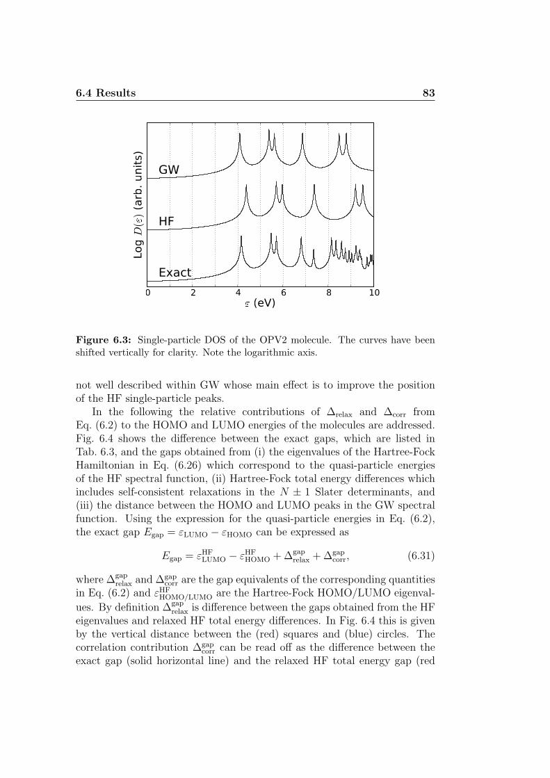
6.4 Results 83
0 2 4 6 8 10ε (eV)
Log D
(
ε) (arb. unit
s)
GW
HF
Exact
Figure 6.3: Single-particle DOS of the OPV2 molecule. The curves have beenshifted vertically for clarity. Note the logarithmic axis.
not well described within GW whose main effect is to improve the positionof the HF single-particle peaks.
In the following the relative contributions of ∆relax and ∆corr fromEq. (6.2) to the HOMO and LUMO energies of the molecules are addressed.Fig. 6.4 shows the difference between the exact gaps, which are listed inTab. 6.3, and the gaps obtained from (i) the eigenvalues of the Hartree-FockHamiltonian in Eq. (6.26) which correspond to the quasi-particle energiesof the HF spectral function, (ii) Hartree-Fock total energy differences whichincludes self-consistent relaxations in the N ± 1 Slater determinants, and(iii) the distance between the HOMO and LUMO peaks in the GW spectralfunction. Using the expression for the quasi-particle energies in Eq. (6.2),the exact gap Egap = εLUMO − εHOMO can be expressed as
Egap = εHFLUMO − εHF
HOMO + ∆gaprelax + ∆gap
corr, (6.31)
where ∆gaprelax and ∆gap
corr are the gap equivalents of the corresponding quantitiesin Eq. (6.2) and εHF
HOMO/LUMO are the Hartree-Fock HOMO/LUMO eigenval-
ues. By definition ∆gaprelax is difference between the gaps obtained from the HF
eigenvalues and relaxed HF total energy differences. In Fig. 6.4 this is givenby the vertical distance between the (red) squares and (blue) circles. Thecorrelation contribution ∆gap
corr can be read off as the difference between theexact gap (solid horizontal line) and the relaxed HF total energy gap (red
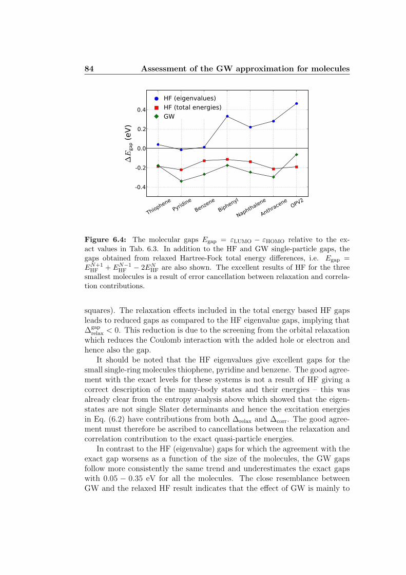
84 Assessment of the GW approximation for molecules
Thiophene
Pyridine
Benzene
Biphenyl
Naphthalene
Anthracene
OPV2
-0.4
-0.2
0.0
0.2
0.4
∆E
gap (
eV
)
HF (eigenvalues)
HF (total energies)
GW
Figure 6.4: The molecular gaps Egap = εLUMO − εHOMO relative to the ex-act values in Tab. 6.3. In addition to the HF and GW single-particle gaps, thegaps obtained from relaxed Hartree-Fock total energy differences, i.e. Egap =EN+1
HF + EN−1HF − 2EN
HF are also shown. The excellent results of HF for the threesmallest molecules is a result of error cancellation between relaxation and correla-tion contributions.
squares). The relaxation effects included in the total energy based HF gapsleads to reduced gaps as compared to the HF eigenvalue gaps, implying that∆gap
relax < 0. This reduction is due to the screening from the orbital relaxationwhich reduces the Coulomb interaction with the added hole or electron andhence also the gap.
It should be noted that the HF eigenvalues give excellent gaps for thesmall single-ring molecules thiophene, pyridine and benzene. The good agree-ment with the exact levels for these systems is not a result of HF giving acorrect description of the many-body states and their energies – this wasalready clear from the entropy analysis above which showed that the eigen-states are not single Slater determinants and hence the excitation energiesin Eq. (6.2) have contributions from both ∆relax and ∆corr. The good agree-ment must therefore be ascribed to cancellations between the relaxation andcorrelation contribution to the exact quasi-particle energies.
In contrast to the HF (eigenvalue) gaps for which the agreement with theexact gap worsens as a function of the size of the molecules, the GW gapsfollow more consistently the same trend and underestimates the exact gapswith 0.05 − 0.35 eV for all the molecules. The close resemblance betweenGW and the relaxed HF result indicates that the effect of GW is mainly to
6.4 Results 85
account for the screening effects that are given by orbital relaxations ∆relax
in HF.
6.4.3 Lattice DFT
To demonstrate the shortcomings DFT when it comes to the interpretationof the Kohn-Sham eigenvalues εKS
i as excitation energies, the spectrum ofthe benzene molecule as obtained with the lattice formulation of DFT [122]is here inspected.
The lattice version of DFT follows by extending the fundamental conceptsof normal DFT, such as the Hohenberg-Kohn theorem and the Kohn-Shamequations, to model Hamiltonians as e.g. the PPP-Hamiltonian. In thisreformulation of DFT the site occupations ni replaces the continuous electrondensity n(r) as the fundamental variable that determines the ground stateproperties. The lattice version of the single-particle Kohn-Sham HamiltonianHKS is given by the sum of the hopping terms (the kinetic energy) and asite dependent Kohn-Sham potential V KS
i which is constructed to yield thecorrect site occupations of the ground state,
HKS = −∑〈ij〉σ
tijc†iσcjσ +
∑i
V KSi ni. (6.32)
For the present purpose the explicit form of the site potential V KSi is not
important. The fact that the lattice version of the Kohn-Sham potential is anonsite potential, is equivalent to the restriction of the Kohn-Sham potentialVxc(r) in the real-space formulation of DFT to a local potential.
Due to the high symmetry of the benzene molecule all sites in the PPP-Hamiltonian are equivalent implying that V KS
i has the same value for all sites.Except for a constant shift, the eigenvalues of the Kohn-Sham Hamiltonianare therefore given by those of the hopping part of the Hamiltonian. TheHOMO-LUMO gap calculated from the Kohn-Sham eigenvalues is EKS
gap =5.08 eV which is a severe underestimation of the true gap of 11.39 eV.
To illustrate why the Kohn-Sham eigenvalues in general seem to consis-tently underestimate molecular gaps, a closer look at the Hartree-Fock Hamil-tonian in Eq. (6.26) is instructive. As Fig. 6.4 showed, HF gave relativelygood values for the gaps reproducing the exact gaps to within ∼ 0.50 eV.The Hartree-Fock Hamiltonian is diagonal in the basis φν of molecularorbitals
HHF =∑νσ
ενσnνσ, (6.33)

86 Assessment of the GW approximation for molecules
with the diagonal elements (eigenvalues) given by
ενσ = tνν +∑µσ′
Vνµnµσ′ − Vννnνσ. (6.34)
Notice that only the direct elements Vννµµ of the Coulomb interaction havebeen included here. Due to the delocalized nature of the molecular orbitalsthis is in general not a good approximation. For the present purpose, how-ever, this suffices to illustrate the point made below.
The exchange contribution to the eigenvalue in the last term removes theself-interaction contribution to the eigenvalue included in the Hartree partin the second term. However, since it depends on the occupation of themolecular orbital itself which is 1 for occupied and 0 for (virtual) unoccu-pied orbitals, only the occupied orbitals are affected by this self-interactioncorrection. This illustrates the orbital dependence of the single-particle HFpotential – i.e. the fact that the HF Hamiltonian differs for occupied andunoccupied orbitals. This distinction between occupied and unoccupied or-bitals, which is a consequence of the non-locality of the HF potential, cannotbe obtained with a local site dependent potential in lattice DFT. The under-estimation of the gap thus seems to be a intrinsic property of the Kohn-Shamformulation of DFT.
For benzene, the molecular orbitals from the non-interacting Hamiltonianand the HF Hamiltonian are identical implying that tνν = εKS
ν . The differencebetween the Kohn-Sham gap and HF gap is thus given by the self-interactioncorrection of the HOMO level.
6.5 Conclusion and outlook
The present chapter has demonstrated that the GW approximation givesconsistently good quasi-particle energies and gaps for the range of moleculeconsidered here. In contrast the gaps obtained from the eigenvalues of thesingle-particle Hartree-Fock Hamiltonian which showed large variations inthe errors, the GW approximation systematically underestimated the molec-ular gaps. The GW results were found to agree well with HF total energycalculations of the gaps in which relaxation of the molecular orbitals for thecharged molecule is taken into account.
Furthermore, the failure of the interpretation of the Kohn-Sham DFTeigenvalues as excitation energies was demonstrated with a simple example.From the lattice version of DFT the gap of the benzene molecule was foundto be severely underestimated by more than a factor of two.
6.5 Conclusion and outlook 87
The GW approximation has recently been extended to non-equilibriumsituations within the framework of the non-equilibrium Green’s function for-malism. It has been applied to quantum transport calculations on single-molecule junction in the strong coupling regime [120, 123, 124], i.e. wherethe hybridization between the molecule and metal contacts is significant. Asthis results in extended states and decreased life-times of molecular states,dynamical polarization effects can be expected to be important in these junc-tions.
So far, first-principles calculations on single-molecule junctions in thestrong coupling regime have almost exclusively been based on DFT descrip-tions of the electronic structure of the junction (see e.g. [125, 126, 127]). How-ever, the zero bias conductance resulting from this approach does typicallynot agree with experimental values and is sometimes orders of magnitudeslarger [128, 129]. The uncertainty connected with the atomic structure of thejunction and the position of the molecule in the experiments is one possiblereason for this discrepancy. Since the conductance of a single-molecule junc-tion is highly dependent on the position of the molecular levels, the use ofDFT in these calculation could be another possible reason for the observeddiscrepancies. Indeed, it has been demonstrated that better agreement withexperiment is obtained by correcting the DFT levels of the molecule to rep-resent true excitation energies [130, 131]. The corrections applied to theDFT levels in these works include (i) a shift of the HOMO level to fit knownexperimental ionization potentials, and (ii) a polarization shift of the levelsequivalent to the polarization integral in Eq. (5.14).
With GW giving a good description of both excitation energies ofmolecules and polarization effects, it will be interesting to follow its devel-opment with respect to transport calculations in the strong coupling regime.Due to the computational requirements of a fully self-consistent GW calcu-lation, such calculations are presently limited to simple junctions with smallmolecules.

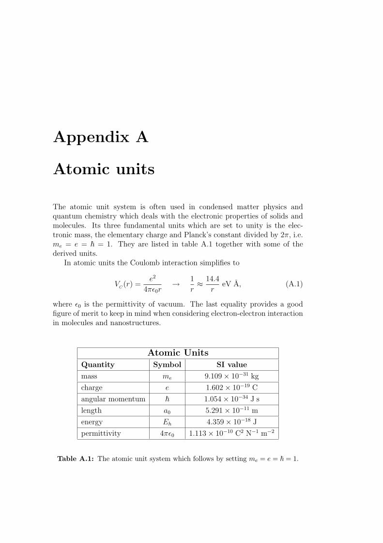
Appendix A
Atomic units
The atomic unit system is often used in condensed matter physics andquantum chemistry which deals with the electronic properties of solids andmolecules. Its three fundamental units which are set to unity is the elec-tronic mass, the elementary charge and Planck’s constant divided by 2π, i.e.me = e = ~ = 1. They are listed in table A.1 together with some of thederived units.
In atomic units the Coulomb interaction simplifies to
VC(r) =
e2
4πε0r→ 1
r≈ 14.4
reV A, (A.1)
where ε0 is the permittivity of vacuum. The last equality provides a goodfigure of merit to keep in mind when considering electron-electron interactionin molecules and nanostructures.
Atomic UnitsQuantity Symbol SI value
mass me 9.109× 10⁻³¹ kg
charge e 1.602× 10⁻¹⁹ C
angular momentum ~ 1.054× 10⁻³⁴ J s
length a0 5.291× 10⁻¹¹ m
energy Eh 4.359× 10⁻¹⁸ J
permittivity 4πε0 1.113× 10⁻¹⁰ C2 N−1 m−2
Table A.1: The atomic unit system which follows by setting me = e = ~ = 1.

Appendix B
Self-consistent Huckel scheme
In this appendix a semi-empirical treatment of the effective single-particlejunction Hamiltonian in Eq. (2.23) is presented. It is based on the extendedHuckel method [132] which has been developed to describe electronic struc-ture of organic molecules. As this method is not self-consistent it is hereextended within the framework of self-consistent Hartree theory. The result-ing self-consistent scheme is similar to the one presented in Ref. [133].
For completeness the single-particle version of the junction Hamiltonianin Eq. (2.23) is given here once more,
Heff = −1
2∇2 + Vion(r) + VH(r) + Vxc(r) + Vind(r) + Vext(r)
= Hmol +Hjunc. (B.1)
Here, the first four terms, which are described together asHmol, stem from themolecule itself. The last two terms included in Hjunc describe the potentialin the junction (see e.g. Chap. 3).
In the self-consistent Huckel scheme the molecular part of the Hamiltonianis written as a sum of a constant term H0 and a self-consistent term HSC
Hmol = H0 +HSC. (B.2)
The constant term H0 accounts for the effective Hamiltonian of the isolatedmolecule. It is approximated by the non-interacting Huckel Hamiltonian
H0 =∑
i
εic†ici +
∑i6=j
tijc†icj, (B.3)
where the sums runs over atomic valence orbitals φi and i is a collectiveindex referring to atom, orbital and spin index. Within Huckel theory the
92 Self-consistent Huckel scheme
onsite energies εi and transfer integrals tij are described with the Hoffmanparametrization [132]
εi = −Vi (B.4)
tij =1
2kSij (εi + εj) . (B.5)
Here, Vi is associated with the ionization energy of the valence orbital φi, k isa fitting parameter usually set to k = 1.75 and Sij = 〈φi|φj〉 is the overlap be-tween the non-orthogonal atomic orbitals. Notice that Hartree and exchange-correlation effects are implicitly included in H0 due to its parametrized form.
The self-consistent term HSC of the molecular Hamiltonian takes intoaccount electron-electron interactions at the level of Hartree theory. It ac-counts for rearrangement of the molecular charge distribution due to addi-tional charges on the molecule and external potentials from the junction.Since the Hartree potential of the isolated molecule is indirectly included inH0, only changes in the Hartree potential due to variations in the electrondensity from its value n0 in the isolated molecule are considered,
δVH(r) =
∫dr′
δn(r′)
|r− r′|. (B.6)
Here δn = n−n0. Since the Hartree potential depends on the electron density,this posses a self-consistent problem that must be iterated to convergence.
To simplify the numerics, the Hartree potential in equation (B.6) is ap-proximated by a sum over atomic point charges given by the Mulliken pop-ulations ni = Tr [ρS]i. The trace is taken over the orbitals on atom i andρ denotes the single-particle density matrix. The matrix elements of thedensity matrix can be expressed in terms of the expansion coefficients cνi tothe molecular orbitals φν as
ρij =∑
ν
(cνi )∗cνj . (B.7)
With the above approximation the Hartree potential reads
δVH(r) =∑
i
δni
|r− ri|. (B.8)
To avoid problems with the diverging point charge potential when evaluatedat the atomic positions, ri, the onsite contribution to the sum is replaced by aspecies dependent Hubbard U taking into account the energy cost of addingan electron to the atom. These parameters are taken from the quantum

93
chemical CNDO method [63, 134]. In order to keep consistency between theonsite and the offsite interactions, the Magata-Nishimoto [135] interpolationformula is used
Uij =1
Rij + 2Ui+Uj
. (B.9)
The final form of the Hartree potential in equation (B.6) becomes
δVH(ri) = δniUi +∑j 6=i
δnjUij. (B.10)
The matrix elements of the Hartree potential in the atomic Huckel basis areapproximated as follows
V Hi = 〈φi|δVH|φi〉 ≈ δVH(ri)
V Hij = 〈φi|δVH|φj〉 ≈
1
2Sij
(V H
i + V Hj
). (B.11)
The matrix elements of the potentials Vind and Vext in the junction part Hjunc
of the Hamiltonian are approximated similarly. The potentials are obtainedfrom a finite element solution to Poisson’s equation.
In the basis of atomic orbitals the effective single-particle Hamiltonian inEq. (B.1) can now be written
Heff =∑
i
εic†ici +
∑i6=j
tijc†icj +
∑i,j
Vijc†icj, (B.12)
where V = VH + Vind + Vext. The total energy can be evaluated from theeigenvalues εν to the effective Hamiltonian as
E =∑
ν
εν −1
2
∑i
[niVH(ri) + (ni − Zi)Vind(ri)] . (B.13)
The last term subtracts contributions to the total energy that are doubledcounted in the eigenvalues. Here Zi denotes the valence of atom i.
The accuracy of the self-consistent Huckel scheme has been addressed bycomparing the calculated gap (see Eq. (4.2)) of the OPV5 molecule with thatobtained from a more accurate DFT calculation using the B3LYP exchange-correlation functional. The comparison showed that the self-consistentHuckel scheme underestimated the gap by 1.2 eV compared to the DFT.The majority of this difference was found to stem from an underestimationof the single-particle HOMO-LUMO gap in the Huckel calculations.


Appendix C
Green’s function primer
Single-particle Green’s functions (GFs) are very useful when considering theelectronic structure of systems. The most important properties of the re-tarded and lesser Green’s functions relevant for the present work are pre-sented here.
The retarded and lesser functions have the following real-space definitions
Gr(rt, r′t′) = −iθ(t− t′)〈ψ(rt), ψ†(r′t′)〉 (C.1)
andG<(rt, r′t′) = i〈ψ†(r′t′)ψ(rt)〉, (C.2)
respectively. For systems in equilibrium the GFs depend only on the timedifference t − t′. Therefore, their Fourier transforms depend on only oneenergy argument ε.
In practical calculations it is often more useful to express the GFs insome convenient basis. Depending on the problem this could be e.g. themomentum-state basis of translationally invariant systems, the Bloch statesof a periodic system, or molecular and atomic orbitals for molecules. In thesebasis the GFs can be written generally as
Grij(t− t′) = −iθ(t− t′)〈ci(t), c†j(t′)〉 (C.3)
andG<
ij(t− t′) = i〈c†j(t′)ci(t)〉 (C.4)
where the creation and annihilation operators create and annihilate electronsin the generic set of basis orbitals φi. They are connected to the real-spacerepresentations above by a simple change of basis.
Being the expectation value of a creation followed by an annihilationoperator, the lesser function contains the single-particle density matrix
ρij = 〈c†icj〉 = −iG<ij(t− t′ = 0) = −i
∫dε
2πG<
ij(ε). (C.5)
96 Green’s function primer
The occupations ni of the basis orbitals are given by the diagonal elementsρii of the density matrix.
A very useful quantity is the spectral function A which is defined by theimaginary part of the retarded Green’s function
A(ε) = − 1
πImGr(ε). (C.6)
In equilibrium the lesser function can be expressed in terms of the spectralfunction and the Fermi distribution nF as
G<(ε) = 2πiA(ε)nF(ε). (C.7)
This relation is the fluctuation-dissipation theorem for the single-particleGreen’s function. Using this relation, the total number of electrons N =∑
i ni of a system follows as
N =∑
i
ρii =∑
i
∫dε Ai(ε)nF(ε). (C.8)
From this expression the density of states D is seen to be given by the sumover the elements of the spectral function
D(ε) =∑
i
Ai(ε). (C.9)
A useful representation of the retarded Green’s function can be obtainedby a spectral decomposition with respect to a complete set of many-bodyeigenstates
H|Ψn〉 = En|Ψn〉. (C.10)
This so-called Lehmann representation follows by inserting the identity 1 =∑n|Ψn〉〈Ψn| in the definition of the retarded Green’s function in Eq. (C.3)
and Fourier transforming,
Grij(ε) =
∑n
[〈ΨN
0 |ci |ΨN+1n 〉〈ΨN+1
n |c†j|ΨN0 〉
ε− (EN+1n − EN
0 ) + iη+〈ΨN
0 |c†j|ΨN−1
n 〉〈ΨN−1n |ci |ΨN
0 〉ε− (EN
0 − EN−1n ) + iη
].
(C.11)For an N -electron system the sum over many-body states |Ψn〉 is restrictedto the states |ΨN±1
n 〉 of the N ±1-electron system. From the Lehmann repre-sentation the poles of the retarded GF are seen to coincide with the electronaddition εn = EN+1
n −EN0 and removal energies εn = EN
0 −EN−1n . Using the
97
identity 1/(ε + iη) = P(1/ε) − iπδ(ε) with P denoting the principal value,the Lehmann representation of the spectral function follows as
Ai(ε) =∑
n
[∣∣∣〈ΨN+1n |c†i |ΨN
0 〉∣∣∣2 δ(ε− εn) +
∣∣∣〈ΨN−1n |ci |ΨN
0 〉∣∣∣2 δ(ε− εn)
](C.12)
Thus, the peaks of the spectral function correspond to the charge excitationsof the system.
Perturbation series in the electron-electron interactions for the GF can beformulated in terms of the time-ordered (zero temperature) Green’s function
Gij(t− t′) = −i〈T [ci(t)c†j(t
′)]〉 (C.13)
where T denotes the time-ordering operator. With the aid of Feynman dia-grams the following Dyson equation for the time-ordered GF can be derivedfrom the perturbation series
G(t− t′) = G0(t− t′) +
∫dt1
∫dt2 G0(t1 − t′)Σ(t2 − t′1)G(t− t2). (C.14)
Here, the quantities are considered as matrices in the basis indices i and jand matrix-multiplication is implied. Σ is the irreducible self-energy whichcontains all Feynman diagrams that cannot be split into two separate partsby cutting a single Green’s function (G0) line. Depending on the definitionof G0, the exact definition of the self-energy varies. In the present workG0 denotes the Hartree GF implying that the Hartree self-energy diagramshould not be included in the definition of Σ.
From the Dyson equation it follows that the full diagrammatic represen-tation of the time-ordered GF is given by all possible combinations of Green’sfunction lines (G0) and self-energy diagrams. In self-consistent schemes likethe GW approximation the self-energy is defined by the full GF G and notG0. Self-consistent schemes therefore include additional diagrams where theGreen’s function lines themselves have self-energy insertions.
The retarded Green’s function obeys a Dyson equation identical to theone above with the time-ordered quantities replaced by their retarded counterparts. In Fourier space this leads to the following solution for the retardedGreen’s function
Gr(ε) = [ε−H0 − Σr(ε)]−1 , (C.15)
where H0 denotes the single-particle Hartree Hamiltonian.


References
[1] International Technology Roadmap for Semiconductors, http://
public.itrs.net.
[2] G. D. Wilk, R. M. Wallace, and J. M. Anthony, High-κ dielectrics:Current status and materials properties considerations, J. Appl. Phys.89(10), 5243 (2001).
[3] A. Javey, H. Kim, M. Brink, Q. Wang, A. Ural, J. Guo, P. McIntyre,P. McEuen, M. Lundstrom, and H. J. Dai, High-κ dielectrics for ad-vanced carbon-nanotube transistors and logic gates, Nature Mat. 1,241 (2002).
[4] D. Natelson, Single-molecule transistors, in Handbook of Organic Elec-tronics and Photonics, edited by H. S. Nalwa, volume 3, pages 1–49,American Scientific Publishers, Stevenson Ranch, CA, 2007.
[5] Z. Bao and J. Locklin, Organic Field-Effect Transistors, CRC Press,Boca Raton, 2007.
[6] E. C. P. Smits, S. G. J. Mathijssen, P. A. van Hal, S. Setayesh, T. C. T.Geuns, K. A. H. A. Mutsaers, E. Cantatore, H. J. Wondergem, O. W.,R. Resel, M. Kemerink, S. Kirchmeyer, A. M. Muzafarov, S. A. Pono-marenko, B. de Boer, and P. W. M. B. . D. M. de Leeuw, Bottom-uporganic integrated circuits, Nature 455, 956 (2008).
[7] S. J. Tans, A. R. M. Verschueren, and C. Dekker, Room-temperaturetransistor based on a single carbon nanotube, Nature 393, 49 (1998).
[8] J. Xiang, W. Lu, Y. Hu, Y. Wu, H. Yan, and C. M. Lieber, Ge/Sinanowire heterostructures as high-performance field-effect transistors,Nature 441, 489 (2006).
[9] Y. Li, F. Qian, J. Xiang, and C. Lieber, Nanowire electronic andoptoelectronic devices, Materials Today 9, 18 (2006).

100 REFERENCES
[10] A. Aviram and M. A. Ratner, Molecular rectifiers, Chem. Phys. Lett.29, 277 (1974).
[11] H. Park, J. Park, A. K. L. Lim, E. H. Anderson, A. P. Alivisatos, andP. L. McEuen, Nanomechanical oscillations in a single-C60 transistor,Nature 407, 57 (2000).
[12] N. P. Guisinger, N. L. Yoder, and M. C. Hersam, Probing charge trans-port at the single-molecule level on silicon by using cryogenic ultra-highvacuum scanning tunneling microscopy, Proc. Natl. Acad. Sci. 102,8838 (2005).
[13] S. Y. Quek, J. B. Neaton, M. S. Hybertsen, E. Kaxiras, , and S. G.Louie, Negative differential resistance in transport through organicmolecules on silicon, Phys. Rev. Lett. 98, 066807 (2007).
[14] A. V. Danilov, S. E. Kubatkin, S. G. Kafanov, K. Flensberg, andT. Bjørnholm, Electron transfer dynamics of bistable single-moleculejunctions, Nano. Lett. 6, 2184 (2006).
[15] A. V. Danilov, P. Hedegard, D. S. Golubev, T. Bjønholm, and S. E.Kubatkin, Nanoelectromechanical switch operating by tunneling of anentire C60 molecule, Nano. Lett. 8, 2393 (2008).
[16] J. Repp, G. Meyer, S. M. Stojkovic, A. Gourdon, and C. Joachim,Molecules on insulating films: Scanning-tunneling microscopy imagingof individual molecular orbitals, Phys. Rev. Lett. 94, 026803 (2005).
[17] L. Gross, F. Mohn, N. Moll, P. Liljeroth, and G. Meyer, The chemicalstructure of a molecule resolved by atomic force microscopy, Science325, 1110 (2009).
[18] D. M. Cardamone, C. A. Stafford, and S. Mazumdar, Controllingquantum transport through a single molecule, Nano. Lett. 6, 2422(2006).
[19] D. Darau, G. Begemann, A. Donarini, and M. Grifoni, Interference ef-fects on the transport characteristics of a benzene single-electron tran-sistor, Phys. Rev. B 79, 235404 (2009).
[20] S. Kubatkin, A. Danilov, M. Hjort, J. Cornil, J.-L. Bredas, N. S.-Hansen, P. Hedegard, and T. Bjørnholm, Single-electron transistor ofa single organic molecule with access to several redox states, Nature425, 698 (2003).

REFERENCES 101
[21] S. J. Tans, M. H. Devoret, H. Dai, A. Thess, R. E. Smalley, L. J.Geerligs, and C. Dekker, Individual single-wall carbon nanotubes asquantum wires, Nature 386, 474 (1997).
[22] D. H. Cobden, M. Bockrath, P. L. McEuen, A. G. Rinzler, and R. E.Smalley, Spin splitting and even-odd effects in carbon nanotubes, Phys.Rev. Lett. 81, 681 (1998).
[23] S. D. Franceschi, J. A. van Dam, E. P. A. M. Bakkers, L. F. Feiner,L. Gurevich, and L. P. Kouwenhoven, Single-electron tunneling in InPnanowires, Appl. Phys. Lett. 83, 344 (2003).
[24] C. Thelander, T. Martensson, M. T. Bjork, B. J. Ohlsson, M. W. Lars-son, L. R. Wallenberg, and L. Samuelson, Single-electron transistorsin heterostructure nanowires, Appl. Phys. Lett. 83, 2052 (2003).
[25] C. Stampfer, E. Schurtenberger, F. Molitor, J. Guttinger, T. Ihn, andK. Ensslin, Tunable Graphene Single Electron Transistor, Nano. Lett.8, 2378 (2008).
[26] W. Lu, Z. Ji, L. Pfeiffer, K. W. West, and A. J. Rimberg, Real-timedetection of electron tunnelling in a quantum dot, Nature 423, 422(2003).
[27] L. P. Kouwenhoven, D. G. Austing, and S. Tarucha, Few-electronquantum dots, Rep. Prog. Phys. 64, 701 (2001).
[28] J. M. Thijssen and H. S. J. van der Zant, Charge transport and single-electron effects in nanoscale systems, Phys. Stat. Sol. (B) 245, 1455(2008).
[29] D. Natelson, L. H. Yu, J. W. Ciszek, Z. K. Keane, and J. M. Tour,Single-molecule transistors: Electron transfer in the solid state, Chem-ical Physics 324, 267 (2006).
[30] C. H. Ahn, A. Bhattacharya, M. D. Ventra, J. N. Eckstein, C. D. Fris-bie, M. E. Gershenson, A. M. Goldman, I. H. Inoue, J. Mannhart, A. J.Millis, A. F. Morpurgo, D. Natelson, and J.-M. Triscone, Electrostaticmodification of novel materials, Rev. Mod. Phys. 78, 1185 (2006).
[31] E. A. Osorio, T. Bjørnholm, J.-M. Lehn, M. Ruben, and H. S. J. van derZant, Single-molecule transport in three-terminal devices, J. Phys.:Condens. Matter 20, 374121 (2008).

102 REFERENCES
[32] K. Moth-Poulsen and T. Bjørnholm, Molecular electronics with singlemolecules in solid-state devices, Nature Nanotech. 4, 551 (2009).
[33] D. R. Strachan, D. E. Johnston, B. S. Guiton, S. S. Datta, P. K. Davies,D. A. Bonnell, and A. T. C. Johnson, Real-time TEM imaging of theformation of crystalline nanoscale gaps, Phys. Rev. Lett. 100, 056805(2008).
[34] A. R. Champagne, A. N. Pasupathy, and D. C. Ralph, Mechanicallyadjustable and electrically gated single-molecule transistors, Nano.Lett. 5, 305 (2005).
[35] R. H. M. Smit, Y. Noat, C. Untiedt, N. D. Lang, M. C. van Hemert, andJ. M. van Ruitenbeek, Measurement of the conductance of a hydrogenmolecule, Nature 419, 906 (2002).
[36] A. Danilov, S. Kubatkin, S. Kafanov, P. Hedegard, N. Stuhr-Hansen,K. Moth-Poulsen, and T. Bjørnholm, Electronic transport in singlemolecule junctions: Control of the molecule-electrode coupling throughintramolecular tunneling barriers, Nano. Lett. 8(1), 1 (2008).
[37] T. Dadosh, Y. Gordin, R. Krahne, I. Kivrich, D. Mahalu, V. Fryd-man, J. Sperling, A. Yacoby, and I. Bar-Joseph, Measurement of theconductance of single conjugated molecules, Nature 436, 677 (2005).
[38] F. Chen, J. He, C. Nuckolls, T. Roberts, J. E. Klare, and S. Lindsay,A molecular switch based on potential-induced changes of oxidationstate, Nano. Lett. 5, 503 (2005).
[39] F. Chen, C. Nuckolls, and S. Lindsay, In situ measurements of oligoani-line conductance: Linking electrochemistry and molecular electronics,Chemical Physics 324, 236 (2006).
[40] X. Li, B. Xu, X. Xiao, X. Yang, L. Zang, and N. Tao, Controllingcharge transport in single molecules using electrochemical gate, Fara-day Discuss. 131, 111 (2006).
[41] D. Ward, N. Grady, C. Levin, N. Halas, Y. Wu, P. Nordlander, , andD. Natelson, Electromigrated nanoscale gaps for surface-enhanced Ra-man spectroscopy, Nano. Lett. 7, 1396 (2007).
[42] D. R. Ward, N. J. Halas, J. W. Ciszek, J. M. Tour, Y. Wu, P. Nord-lander, and D. Natelson, Simultaneous measurements of electronicconduction and raman response in molecular junctions, Nano. Lett. 8,919 (2008).

REFERENCES 103
[43] R. Hesper, L. H. Tjeng, and G. A. Sawatzky, Strongly reduced bandgap in a correlated insulator in close proximity to a metal, Europhys.Lett. 40(2), 177 (1997).
[44] R. A. Marcus, On the theory of oxidation-reduction reactions involvingelectron transfer. I, J. Chem. Phys. 24, 966 (1956).
[45] M. Pope and C. E. Swenberg, Electronic Processes in Organic Crystalsand Polymers, Oxford University Press, Oxford, 1999.
[46] H. B. Heersche, Z. de Groot, J. A. Folk, H. S. J. van der Zant,C. Romeike, M. R. Wegewijs, L. Zobbi, D. Barreca, E. Tondello, andA. Cornia, Electron transport through single M12 molecular magnets,Phys. Rev. Lett. 96, 206801 (2006).
[47] M.-H. Jo, J. E. Grose, K. Baheti, M. M. Deshmukh, J. J. Sokol, E. M.Rumberger, D. N. Hendrickson, J. R. Long, H. Park, , and D. C. Ralph,Signatures of molecular magnetism in single-molecule transport spec-troscopy, Nano. Lett. 6, 2014 (2006).
[48] J. E. Grose, E. S. Tam, C. Timm, M. Scheloske, B. Ulgut, J. J. Parks,H. D. Abruna, W. Harneit, and D. C. Ralph, Tunnelling spectra of in-dividual magnetic endofullerene molecules, Nature Mat. 7, 884 (2008).
[49] E. A. Osorio, K. O’Neill, M. Wegewijs, N. Stuhr-Hansen, J. Paaske,T. Bjørnholm, and H. S. J. van der Zant, Electronic excitations ofa single molecule contacted in a three-terminal configuration, Nano.Lett. 7(11), 3336 (2007).
[50] E. A. Osorio, K. O’Neill, N. Stuhr-Hansen, O. F. Nielsen,T. Bjørnholm, and H. S. J. van der Zant, Addition energies and vi-brational fine structure measured in electromigrated single-moleculejunctions based on an oligophenylenevinylene derivative, Adv. Mater.19(2), 281 (2007).
[51] A. N. P. J. Park, J. I. Goldsmith, C. Chang, Y. Yaish, J. R. Petta,M. Rinkoski, J. P. Sethna, H. D. Abruna, and P. L. McEuen, Coulombblockade and the Kondo effect in single-atom transistors, Nature 417,722 (2002).
[52] L. H. Yu and D. Natelson, The Kondo effect in C60 single-moleculetransistors, Nano. Lett. 4, 79 (2004).
104 REFERENCES
[53] S. Braig and K. Flensberg, Vibrational sidebands and dissipative tun-neling in molecular transistors, Phys. Rev. B 68, 205324 (2003).
[54] J. Koch, F. von Oppen, and A. V. Andreev, Theory of the Franck-Condon blockade regime, Phys. Rev. B 74, 205438 (2006).
[55] H. Bruus and K. Flensberg, Many-Body Quantum Theory in CondensedMatter Physics: An Introduction, Oxford University Press, Oxford,2004.
[56] S. Lakshmi, S. Dutta, and S. K. Pati, Molecular Electronics: Effect ofexternal electric field, J. Phys. Chem. C 112, 14718 (2008).
[57] L. D. Hallam, J. Weis, and P. A. Maksym, Screening of the electron-electron interaction by gate electrodes in semiconductor quantum dots,Phys. Rev. B 53, 1452 (1996).
[58] P. Hedegard and T. Bjørnholm, Charge transport through imagecharged stabilized states in a single molecule single electron transistordevice, Chemical Physics 319, 350 (2005).
[59] J. D. Sau, J. B. Neaton, H. J. Choi, S. G. Louie, and M. L. Cohen,Electronic energy levels of weakly coupled nanostructures: C60-metalinterfaces, Phys. Rev. Lett. 101, 026804 (2008).
[60] R. Stadler, V. Geskin, and J. Cornil, Screening effects in a density func-tional theory based description of molecular junctions in the Coulombblockade regime, Phys. Rev. B 79, 113408 (2009).
[61] A. C. Maggs and R. Everaers, Simulating nanoscale dielectric response,Phys. Rev. Lett. 96, 230603 (2006).
[62] J. D. Jackson, Classical Electrodynamics, John Wiley & Sons, NewYork, 2 edition, 1975.
[63] P. Fulde, Electron Correlations in Molecules and Solids, Number 100in Springer Series in Solid-State Sciences, Springer, Berlin, 3 edition,1995.
[64] T. Ihn, Electronic Quantum Transport in Mesoscopic SemiconductorStructures, Springer, New York, 2004.
[65] FEniCS, FEniCS Project, http//www.fenics.org/, 2007.
REFERENCES 105
[66] Y. Saad, Iterative methods for sparse linear systems, SIAM, 2 edition,2003.
[67] J. S. Seldenthuis, H. S. J. van der Zant, M. A. Ratner, and J. M.Thijssen, Vibrational excitations in weakly coupled single-moleculejunctions: A computational analysis, ACS Nano 2(7), 1445 (2008).
[68] S. C. Lam and R. J. Needs, First-principles calculation of the screeningof electric fields at the aluminium(111) and (110) surfaces, J. Phys.:Condens. Matter 5(14), 2101 (1993).
[69] E. V. Chulkov, V. M. Silkin, and P. M. Echenique, Image potentialstates on metal surfaces: binding energies and wave functions, Surf.Sci. 437, 330 (1999).
[70] S. S. Datta, D. R. Strachan, and A. T. C. Johnson, Gate coupling tonanoscale electronics, Phys. Rev. B 79, 205404 (2009).
[71] V. M. Geskin, J. Cornil, and J. L. Bredas, Comment on ’Polaronformation and symmetry breaking’ by L. Zuppiroli et al., Chem. Phys.Lett. 403, 228 (2005).
[72] W. Barford, R. J. Bursill, and M. Y. Lavrentiev, Density matrixrenormalization group calculations of the low-lying excitations and non-linear optical properties of poly( para-phenylene), J. Phys.: Condens.Matter 10, 6429 (1998).
[73] X.-Y. Zhu, Charge transport at metal-molecule interfaces: A spectro-scopic view, J. Phys. Chem. B 108(26), 8778 (2004).
[74] E. V. Tsiper, Z. G. Soos, W. Gao, and A. Kahn, Electronic polariza-tion at surfaces and thin films of organic molecular crystals: PTCDA,Chem. Phys. Lett. 360, 47 (2002).
[75] X. Lu, M. Grobis, K. H. Khoo, S. G. Louie, and M. F. Crommie, Chargetransfer and screening in individual C60 molecules on metal substrates:A scanning tunneling spectroscopy and theoretical study, Phys. Rev.B 70, 115418 (2004).
[76] J. B. Neaton, M. S. Hybertsen, and S. G. Louie, Renormalization ofmolecular electronic levels at metal-molecule interfaces, Phys. Rev.Lett. 97, 216405 (2006).
106 REFERENCES
[77] C. Freysoldt, P. Rinke, and M. Scheffler, Controlling polarization atinsulating surfaces: Quasiparticle calculations for molecules adsorbedon insulator films, Phys. Rev. Lett. 103, 056803 (2009).
[78] J. M. Garcia-Lastra, A. Rubio, and K. S. Thygesen, Image chargeeffects and level alignment at solid-molecule interfaces, unpublished(2009).
[79] K. S. Thygesen and A. Rubio, Renormalization of molecular quasipar-ticle levels at metal-molecule interfaces: Trends across binding regimes,Phys. Rev. Lett. 102, 046802 (2009).
[80] J. C. Inkson, Many-body effects at metal-semiconductor junctions: II.The self energy and band structure distortion, J. Phys. C 6, 1350(1973).
[81] J. P. A. Charlesworth, R. W. Godby, and R. J. Needs, First-principlescalculations of many-body band-gap narrowing at an Al/GaAs(110)interface, Phys. Rev. Lett. 70(11), 1685 (1993).
[82] D. O. Demchenko and L.-W. Wang, Localized electron states near ametal/semiconductor nanocontact, Nano. Lett. 7(10), 3219 (2007).
[83] J.-W. van der Horst, P. A. Bobbert, M. A. J. Michels, G. Brocks, andP. J. Kelly, Ab initio calculation of the electronic and optical excitationsin polythiophene: Effects of intra- and interchain screening, Phys. Rev.Lett. 83, 4413 (1999).
[84] Y. Li, D. Lu, and G. Galli, Calculation of quasi-particle energies ofaromatic self-assembled monolayers on Au(111), J. Chem. TheoryComput. 5, 881 (2009).
[85] L. Hedin, New method for calculating the one-particle Green’s functionwith application to the electron-gas problem, Phys. Rev. 139, A796(1965).
[86] L. Hedin and S. Lundquist, Effects of Electron-Electron and Electron-Phonon Interactions on the One-Electron States of Solids, in Solid StatePhysics, edited by F. Seitz, D. Turnbull, and H. Ehrenreich, volume 23,page 1, Academic Press, New York, 1969.
[87] G. Baym and L. P. Kadanoff, Conservation Laws and CorrelatoinFunctions, Phys. Rev. 124(2), 287 (1961).
REFERENCES 107
[88] G. Baym, Self-consistent approximations in many-body systems, Phys.Rev. 127(4), 1391 (1962).
[89] L. Kadanoff and G. Baym, Quantum Statistical Mechanics, W. A.Benjamin, New York, 1962.
[90] B. Holm and U. von Barth, Fully self-consistent GW self-energy of theelectron gas, Phys. Rev. B 57, 2108 (1998).
[91] G. Pal, Y. Pavlyukh, H. C. Schneider, and W. Hubner, Conservingquasiparticle calculations for small metal clusters, Eur. Phys. J. B 70,483 (2009).
[92] W. G. Aulbur, L. Jonsson, and J. W. Wilkins, Quasiparticle calcu-lations in solids, in Solid State Physics, edited by H. Ehrenreich andF. Saepen, volume 54, page 1, Academic Press, New York, 2000.
[93] F. Aryasetiawan and O. Gunnarsson, The GW method, Rep. Prog.Phys. 61, 237 (1998).
[94] G. Onida, L. Reining, and A. Rubio, Electronic excitations: density-functional versus many-body Green’s-function approaches, Rev. Mod.Phys. 74, 601 (2002).
[95] N. Lang and W. Kohn, Theory of metal surfaces: Induced surfacecharge and image potential, Phys. Rev. B 7, 3541 (1973).
[96] J. C. Grossman, M. Rohlfing, L. Mitas, S. G. Louie, and M. L. Cohen,High Accuracy Many-Body Calculational Approaches for Excitationsin Molecules, Phys. Rev. Lett. 86, 472 (2001).
[97] A. Stan, N. E. Dahlen, and R. van Leeuwen, Fully self-consistent GWcalculations for atoms and molecules, Europhys. Lett. 76, 298 (2006).
[98] M. L. Tiago, P. R. C. Kent, R. Q. Hood, and F. A. Reboredo, Neutraland charged excitations in carbon fullerenes from first-principles many-body theories, J. Chem. Phys. 129, 084311 (2008).
[99] C. D. Spataru, S. Ismail-Beigi, X. L. Benedict, and S. G. Louie, Exci-tonic Effects and Optical Spectra of Single-Walled Carbon Nanotubes,Phys. Rev. Lett. 92, 077402 (2004).
[100] P. E. Trevisanutto, C. Giorgetti, L. Reining, M. Ladisa, and V. Ole-vano, Ab initio GW many-body effects in graphene, Phys. Rev. Lett.101, 226405 (2008).

108 REFERENCES
[101] M. L. Tiago and J. R. Chelikowsky, Optical excitations inorganicmolecules, clusters, and defects studied by first-principles Green’s func-tion methods, Phys. Rev. B 73, 205334 (2006).
[102] P. H. Hahn, W. G. Schmidt, and F. Bechstedt, Molecular electronicexcitations calculated from a solid-state approach: Methodology andnumerics, Phys. Rev. B 72, 245425 (2005).
[103] C. Verdozzi, R. W. Godby, and S. Holloway, Evaluation of GW ap-proximations for the self-energy of a Hubbard cluster, Phys. Rev. Lett.74, 2327 (1995).
[104] T. J. Pollehn, A. Schindlmayr, and R. W. Godby, Assessment of theGW approximation using Hubbard chains, J. Phys.: Condens. Matter10, 1273 (1998).
[105] A. Schindlmayr, T. T. Pollehn, and R. W. Godby, Spectra and totalenergies from self-consistent many-body perturbation theory, Phys.Rev. B 58, 12684 (1998).
[106] M. P. von Friesen, C. Verdozzi, and C.-O. Almbladh, Successes andfailures of Kadanoff-Baym dynamics in Hubbard nanoclusters, Phys.Rev. Lett. 103, 176404 (2009).
[107] J. A. Pople, Electron interaction in unsaturated hydrocarbons, Trans.Faraday Soc. 49, 1375 (1953).
[108] R. Pariser and R. G. Parr, A semi-empirical theory of the electronicspectra and electronic structure of complex unsaturated molecules .2,J. Chem. Phys. 21(5), 466 (1953).
[109] R. Pariser and R. G. Parr, A semi-empirical theory of the electronicspectra and electronic structure of complex unsaturated molecules .2,J. Chem. Phys. 21(5), 767 (1953).
[110] K. Ohno, The present status of the theory of molecular electronicstructure - Semiempirical methods, Theor. Chim. Acc. 2, 219 (1964).
[111] I. R. Ducasse, T. E. Miller, and Z. G. Soos, Correlated states in finitepolyenes: Exact PPP results, J. Chem. Phys. 76, 4094 (1982).
[112] W. Barford and R. J. Bursill, Theory of molecular excitons in thephenyl-based organic semiconductors, Chem. Phys. Lett. 268, 535(1997).

REFERENCES 109
[113] R. J. Bursill, C. Castleton, and W. Barford, Optimal parametrisationof the Pariser-Parr-Pople model for benzene and biphenyl, Chem. Phys.Lett. 294, 305 (1998).
[114] W. Barford, R. J. Bursill, and M. Y. Lavrentiev, Density matrixrenormalization group calculations of the low-lying excitations and non-linear optical properties of poly (para-phenylene), J. Phys.: Condens.Matter 10, 6429 (1998).
[115] M. Y. Lavrentiev, W. Barford, S. J. Martin, and H. Daly, Theoreticalinvestigation of the low-lying electronic structure of poly(p-phenylenevinylene), Phys. Rev. B 59(15), 9987 (1999).
[116] S. Yamada, T. Imamura, and M. Machida, 16.447 TFlops and 159-billion-dimensional exact-diagonalization for trapped fermion-Hubbardmodel on the Earth Simulator, SC Conference 0, 44 (2005).
[117] P. Dayal, M. Troyer, and R. Villiger, The Iterative Eigensolver Tem-plate Library (IETL), http://www.comp-phys.org/software/ietl/.
[118] J. K. Cullum and R. A. Willoughby, Lanczos Algorithms for LargeSymmetric Eigenvalue Computations, volume 1, SIAM, 2002.
[119] E. Dagotto, Correlated electrons in high-temperature superconductors,Rev. Mod. Phys. 66(3), 763 (1994).
[120] K. S. Thygesen and A. Rubio, Conserving GW scheme for nonequi-librium quantum transport in molecular contacts, Phys. Rev. B 77,115333 (2008).
[121] A. L. Fetter and J. D. Walecka, Quantum theory of many-particlesystems, McGraw-Hill, New York, 1971.
[122] K. Schonhammer, O. Gunnarsson, and R. M. Noack, Density-functional theory on a lattice: Comparison with exact numerical resultsfor a model with strongly correlated electrons, Phys. Rev. B 52, 2504(1995).
[123] K. S. Thygesen and A. Rubio, Nonequilibrium GW approach to quan-tum transport in nano-scale contacts, J. Chem. Phys. 126, 091101(2007).
[124] P. Darancet, A. Ferretti, D. Mayou, and V. Olevano, Ab initio GWelectron-electron interaction effects in quantum transport, Phys. Rev.B 75, 075102 (2007).
110 REFERENCES
[125] P. S. Damle, A. W. Ghosh, and S. Datta, Unified description of molec-ular conduction: From molecules to metallic wires, Phys. Rev. B 64,201403 (2001).
[126] J. Taylor, M. Brandbyge, and K. Stokbro, Theory of rectification intour wires: The role of electrode coupling, Phys. Rev. Lett. 89, 138301(2002).
[127] K. S. Thygesen and K. W. Jacobsen, Conduction mechanism in amolecular hydrogen contact, Phys. Rev. Lett. 94, 036807 (2005).
[128] M. D. Ventra, S. T. Pantelides, and N. D. Lang, First-principles calcu-lation of transport properties of a molecular device, Phys. Rev. Lett.84, 979 (2000).
[129] Y. Xue and M. A. Ratner, Theoretical principles of single-moleculeelectronics: A chemical and mesoscopic view, Int. J. Quantum Chem.102, 911 (2005).
[130] D. J. Mowbray, G. Jones, and K. S. Thygesen, Influence of functionalgroups on charge transport in molecular junctions, J. Chem. Phys.128, 111103 (2008).
[131] S. Y. Quek, L. Venkataraman, H. J. Choi, S. G. Louie, M. S. Hy-bertsen, and J. B. Neaton, Amine-gold linked single-molecule circuits:Experiment and theory, Nano. Lett. 7(11), 3477 (2007).
[132] R. Hoffmann, An Extended Huckel theory. I. Hydrocarbons, J. Chem.Phys. 39, 1397 (1963).
[133] F. Zahid, M. Paulsson, E. Polizzi, A. W. Ghosh, L. Siddiqui, andS. Datta, A self-consistent transport model for molecular conductionbased on extended Huckel theory with full three-dimensional electro-statics, J. Chem. Phys. 123(6), 064707 (2005).
[134] J. A. Pople and G. A. Segal, Approximate Self-Consistent MolecularOrbital Theory. III. CNDO Results for AB2 and AB3 Systems, J.Chem. Phys. 44, 3289 (1966).
[135] J. M. Sichel and M. A. Whitehead, Semi-Empirical All Valence Elec-trons SCF-LCAO-MO Theory, Theor. Chim. Acc. 11, 220 (1968).


Paper I

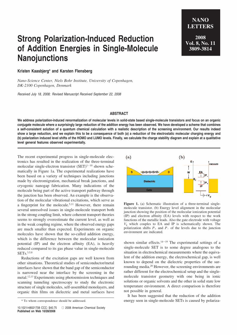
Strong Polarization-Induced Reductionof Addition Energies in Single-MoleculeNanojunctionsKristen Kaasbjerg* and Karsten Flensberg
Nano-Science Center, Niels Bohr Institute, UniVersity of Copenhagen,DK-2100 Copenhagen, Denmark
Received July 18, 2008; Revised Manuscript Received September 22, 2008
ABSTRACT
We address polarization-induced renormalization of molecular levels in solid-state based single-molecule transistors and focus on an organicconjugate molecule where a surprisingly large reduction of the addition energy has been observed. We have developed a scheme that combinesa self-consistent solution of a quantum chemical calculation with a realistic description of the screening environment. Our results indeedshow a large reduction, and we explain this to be a consequence of both (a) a reduction of the electrostatic molecular charging energy and(b) polarization induced level shifts of the HOMO and LUMO levels. Finally, we calculate the charge stability diagram and explain at a qualitativelevel general features observed experimentally.
The recent experimental progress in single-molecule elec-tronics has resulted in the realization of the three-terminalmolecular single-electron transistor (SET)1-10 shown sche-matically in Figure 1a. The experimental realizations havebeen based on a variety of techniques including junctionsmade by electromigration, mechanical break junctions, andcryogenic nanogap fabrication. Many indications of themolecule being part of the active transport pathway throughthe junction has been observed. An example is the observa-tion of the molecular vibrational excitations, which serve asa fingerprint for the molecule.5,11 However, there remainseveral unresolved issues in single-molecule transport bothin the strong coupling limit, where coherent transport theoriesseems to strongly overestimate the current level, as well asin the weak coupling regime, where the observed energy gapsare much smaller than expected. Experiments on organicmolecules have shown that the so-called addition energy,which is the difference between the molecular ionizationpotential (IP) and the electron affinity (EA), is heavilyreduced compared to its gas phase value in single-moleculeSETs.3,5,8
Reductions of the excitation gaps are well known fromother situations. Theoretical studies of semiconductor/metalinterfaces have shown that the band gap of the semiconductoris narrowed near the interface by the screening in themetal.12,13 Experiments using photoemission techniques andscanning tunneling spectroscopy to study the electronicstructure of single molecules, self-assembled monolayers, andorganic thin films on dielectric and metal surfaces have
shown similar effects.14-19 The experimental settings of asingle-molecule SET is to some degree analogous to thesituation in electrochemical measurements where the equiva-lent of the addition energy, the electrochemical gap, is wellknown to depend on the dielectric properties of the sur-rounding media.20 However, the screening environments arerather different for the electrochemical setup and the single-molecule transistor geometry with one being in ionicsolutions or organic solvents and the other in solid state lowtemperature environment. A direct comparison is thereforenot possible in general.
It has been suggested that the reduction of the additionenergy seen in single-molecule SETs is caused by polariza-* To whom correspondence should be addressed.
Figure 1. (a) Schematic illustration of a three-terminal single-molecule transistor. (b) Energy level alignment in the molecularjunction showing the position of the molecular ionization potential(IP) and electron affinity (EA) levels with respect to the workfunctions of the metallic leads. Also the gate electrode with voltageVg which couples to EA and IP is schematically shown. Thepolarization shifts P+ and P- of the levels due to the junctionenvironment are indicated.
NANOLETTERS
2008Vol. 8, No. 11
3809-3814
10.1021/nl8021708 CCC: $40.75 2008 American Chemical SocietyPublished on Web 10/28/2008
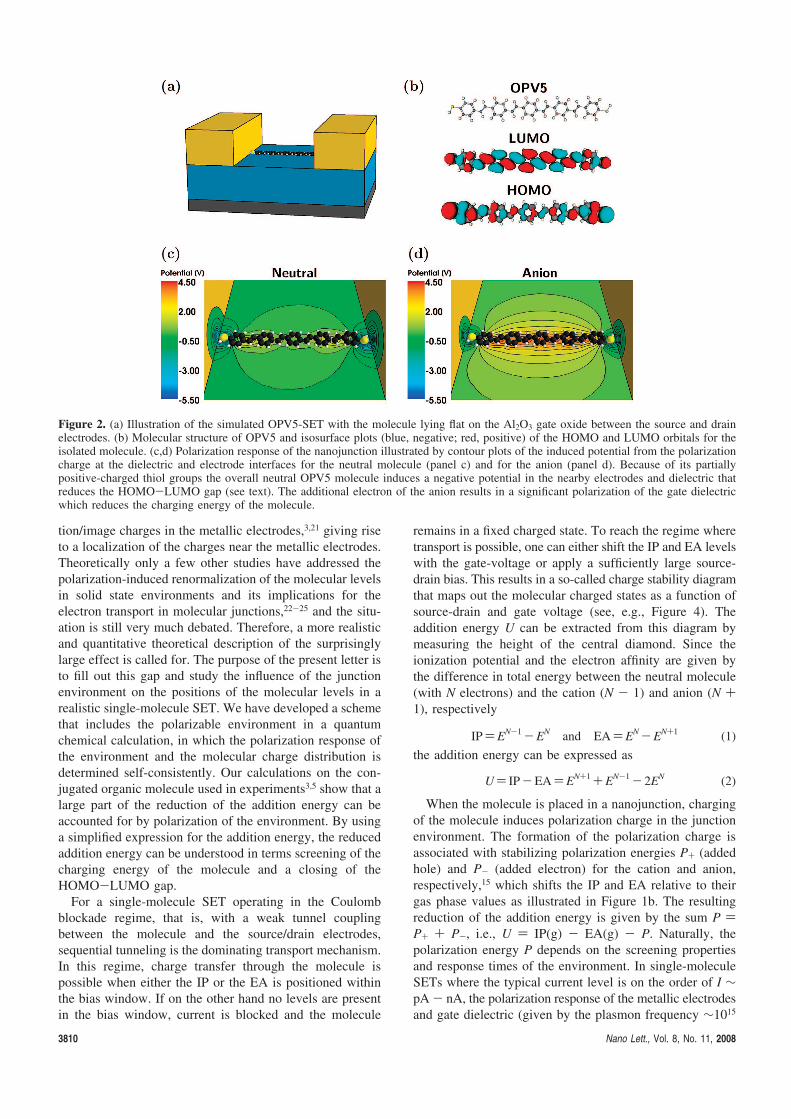
tion/image charges in the metallic electrodes,3,21 giving riseto a localization of the charges near the metallic electrodes.Theoretically only a few other studies have addressed thepolarization-induced renormalization of the molecular levelsin solid state environments and its implications for theelectron transport in molecular junctions,22-25 and the situ-ation is still very much debated. Therefore, a more realisticand quantitative theoretical description of the surprisinglylarge effect is called for. The purpose of the present letter isto fill out this gap and study the influence of the junctionenvironment on the positions of the molecular levels in arealistic single-molecule SET. We have developed a schemethat includes the polarizable environment in a quantumchemical calculation, in which the polarization response ofthe environment and the molecular charge distribution isdetermined self-consistently. Our calculations on the con-jugated organic molecule used in experiments3,5 show that alarge part of the reduction of the addition energy can beaccounted for by polarization of the environment. By usinga simplified expression for the addition energy, the reducedaddition energy can be understood in terms screening of thecharging energy of the molecule and a closing of theHOMO-LUMO gap.
For a single-molecule SET operating in the Coulombblockade regime, that is, with a weak tunnel couplingbetween the molecule and the source/drain electrodes,sequential tunneling is the dominating transport mechanism.In this regime, charge transfer through the molecule ispossible when either the IP or the EA is positioned withinthe bias window. If on the other hand no levels are presentin the bias window, current is blocked and the molecule
remains in a fixed charged state. To reach the regime wheretransport is possible, one can either shift the IP and EA levelswith the gate-voltage or apply a sufficiently large source-drain bias. This results in a so-called charge stability diagramthat maps out the molecular charged states as a function ofsource-drain and gate voltage (see, e.g., Figure 4). Theaddition energy U can be extracted from this diagram bymeasuring the height of the central diamond. Since theionization potential and the electron affinity are given bythe difference in total energy between the neutral molecule(with N electrons) and the cation (N - 1) and anion (N +1), respectively
IP)EN-1 -EN and EA)EN -EN+1 (1)
the addition energy can be expressed as
U) IP-EA)EN+1 +EN-1 - 2EN (2)
When the molecule is placed in a nanojunction, chargingof the molecule induces polarization charge in the junctionenvironment. The formation of the polarization charge isassociated with stabilizing polarization energies P+ (addedhole) and P- (added electron) for the cation and anion,respectively,15 which shifts the IP and EA relative to theirgas phase values as illustrated in Figure 1b. The resultingreduction of the addition energy is given by the sum P )P+ + P-, i.e., U ) IP(g) - EA(g) - P. Naturally, thepolarization energy P depends on the screening propertiesand response times of the environment. In single-moleculeSETs where the typical current level is on the order of I ∼pA - nA, the polarization response of the metallic electrodesand gate dielectric (given by the plasmon frequency ∼1015
Figure 2. (a) Illustration of the simulated OPV5-SET with the molecule lying flat on the Al2O3 gate oxide between the source and drainelectrodes. (b) Molecular structure of OPV5 and isosurface plots (blue, negative; red, positive) of the HOMO and LUMO orbitals for theisolated molecule. (c,d) Polarization response of the nanojunction illustrated by contour plots of the induced potential from the polarizationcharge at the dielectric and electrode interfaces for the neutral molecule (panel c) and for the anion (panel d). Because of its partiallypositive-charged thiol groups the overall neutral OPV5 molecule induces a negative potential in the nearby electrodes and dielectric thatreduces the HOMO-LUMO gap (see text). The additional electron of the anion results in a significant polarization of the gate dielectricwhich reduces the charging energy of the molecule.
3810 Nano Lett., Vol. 8, No. 11, 2008
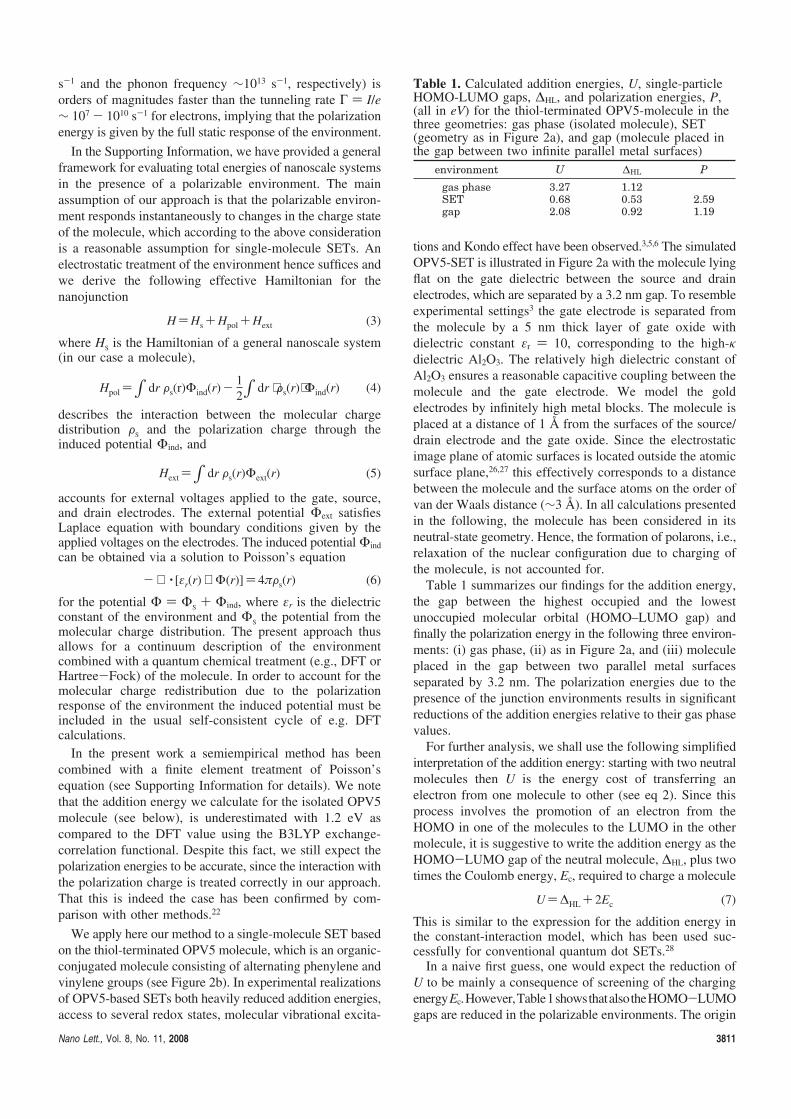
s-1 and the phonon frequency ∼1013 s-1, respectively) isorders of magnitudes faster than the tunneling rate Γ ) I/e∼ 107 - 1010 s-1 for electrons, implying that the polarizationenergy is given by the full static response of the environment.
In the Supporting Information, we have provided a generalframework for evaluating total energies of nanoscale systemsin the presence of a polarizable environment. The mainassumption of our approach is that the polarizable environ-ment responds instantaneously to changes in the charge stateof the molecule, which according to the above considerationis a reasonable assumption for single-molecule SETs. Anelectrostatic treatment of the environment hence suffices andwe derive the following effective Hamiltonian for thenanojunction
H)Hs +Hpol +Hext (3)
where HS is the Hamiltonian of a general nanoscale system(in our case a molecule),
Hpol )∫ dr Fs(r)Φind(r)- 12∫ dr ⟨Fs(r)⟩Φind(r) (4)
describes the interaction between the molecular chargedistribution FS and the polarization charge through theinduced potential Φind, and
Hext )∫ dr Fs(r)Φext(r) (5)
accounts for external voltages applied to the gate, source,and drain electrodes. The external potential Φext satisfiesLaplace equation with boundary conditions given by theapplied voltages on the electrodes. The induced potential Φind
can be obtained via a solution to Poisson’s equation
- ∇ · [εr(r) ∇ Φ(r)]) 4πFs(r) (6)
for the potential Φ ) ΦS + Φind, where εr is the dielectricconstant of the environment and ΦS the potential from themolecular charge distribution. The present approach thusallows for a continuum description of the environmentcombined with a quantum chemical treatment (e.g., DFT orHartree-Fock) of the molecule. In order to account for themolecular charge redistribution due to the polarizationresponse of the environment the induced potential must beincluded in the usual self-consistent cycle of e.g. DFTcalculations.
In the present work a semiempirical method has beencombined with a finite element treatment of Poisson’sequation (see Supporting Information for details). We notethat the addition energy we calculate for the isolated OPV5molecule (see below), is underestimated with 1.2 eV ascompared to the DFT value using the B3LYP exchange-correlation functional. Despite this fact, we still expect thepolarization energies to be accurate, since the interaction withthe polarization charge is treated correctly in our approach.That this is indeed the case has been confirmed by com-parison with other methods.22
We apply here our method to a single-molecule SET basedon the thiol-terminated OPV5 molecule, which is an organic-conjugated molecule consisting of alternating phenylene andvinylene groups (see Figure 2b). In experimental realizationsof OPV5-based SETs both heavily reduced addition energies,access to several redox states, molecular vibrational excita-
tions and Kondo effect have been observed.3,5,6 The simulatedOPV5-SET is illustrated in Figure 2a with the molecule lyingflat on the gate dielectric between the source and drainelectrodes, which are separated by a 3.2 nm gap. To resembleexperimental settings3 the gate electrode is separated fromthe molecule by a 5 nm thick layer of gate oxide withdielectric constant εr ) 10, corresponding to the high-κdielectric Al2O3. The relatively high dielectric constant ofAl2O3 ensures a reasonable capacitive coupling between themolecule and the gate electrode. We model the goldelectrodes by infinitely high metal blocks. The molecule isplaced at a distance of 1 Å from the surfaces of the source/drain electrode and the gate oxide. Since the electrostaticimage plane of atomic surfaces is located outside the atomicsurface plane,26,27 this effectively corresponds to a distancebetween the molecule and the surface atoms on the order ofvan der Waals distance (∼3 Å). In all calculations presentedin the following, the molecule has been considered in itsneutral-state geometry. Hence, the formation of polarons, i.e.,relaxation of the nuclear configuration due to charging ofthe molecule, is not accounted for.
Table 1 summarizes our findings for the addition energy,the gap between the highest occupied and the lowestunoccupied molecular orbital (HOMO–LUMO gap) andfinally the polarization energy in the following three environ-ments: (i) gas phase, (ii) as in Figure 2a, and (iii) moleculeplaced in the gap between two parallel metal surfacesseparated by 3.2 nm. The polarization energies due to thepresence of the junction environments results in significantreductions of the addition energies relative to their gas phasevalues.
For further analysis, we shall use the following simplifiedinterpretation of the addition energy: starting with two neutralmolecules then U is the energy cost of transferring anelectron from one molecule to other (see eq 2). Since thisprocess involves the promotion of an electron from theHOMO in one of the molecules to the LUMO in the othermolecule, it is suggestive to write the addition energy as theHOMO-LUMO gap of the neutral molecule, ∆HL, plus twotimes the Coulomb energy, Ec, required to charge a molecule
U)∆HL + 2Ec (7)
This is similar to the expression for the addition energy inthe constant-interaction model, which has been used suc-cessfully for conventional quantum dot SETs.28
In a naive first guess, one would expect the reduction ofU to be mainly a consequence of screening of the chargingenergyEc.However,Table1showsthatalsotheHOMO-LUMOgaps are reduced in the polarizable environments. The origin
Table 1. Calculated addition energies, U, single-particleHOMO-LUMO gaps, ∆HL, and polarization energies, P,(all in eV) for the thiol-terminated OPV5-molecule in thethree geometries: gas phase (isolated molecule), SET(geometry as in Figure 2a), and gap (molecule placed inthe gap between two infinite parallel metal surfaces)
environment U ∆HL P
gas phase 3.27 1.12SET 0.68 0.53 2.59gap 2.08 0.92 1.19
Nano Lett., Vol. 8, No. 11, 2008 3811

of this reduction is illustrated in Figure 2c. Because of thepositively charged thiol groups of the overall neutral OPV5,a negative electrostatic potential is induced in the nearbyelectrodes and dielectric. This, combined with the localizationof the HOMO on the thiol groups (see Figure 2b), shifts theHOMO level to higher energy. Similar reasoning for thenegatively charged carbon backbone and the LUMO leadsto a lowering of the LUMO level and hence a closing of theHOMO-LUMO gap. The charging energy obtained fromeq 7 is for OPV5 in gas phase Ec ) 1.08 eV. The screeningresponse of the nanojunction, which is shown for the OPV5anion in Figure 2d, reduces this value to Ec ) 75 meV. Tosummarize, we can understand the reduction of the additionenergy as a consequence of two parallel effects: (i) areduction of the HOMO-LUMO gap and (ii) screening ofthe Coulomb repulsion on the molecule which lowers thecharging energy. Since the majority of the reduction is dueto the latter effect, which is purely electrostatic in nature,the reduction for other molecules of the same size of OPV5will be comparable. For smaller molecules we have foundthat the closer proximity of the polarization charge enhancesthe screening of the charging energy, resulting in largerabsolute reductions.
The important role of the gate oxide in the reduction of Uis clearly demonstrated by the large difference in thepolarization energy between the SET and gap environmentin Table 1. More than half of the polarization energy of 2.59eV in the SET environment is due to the gate oxide. As themolecule is lying flat on the oxide which has almost metallic-like screening properties (the image charge strength of adielectric surface is qεr ) (εr - 1)/(εr + 1)), this should comeas no surprise. Note that the polarization energy in the SETenvironment is highly dependent on the dielectric constantof the gate oxide. With a SiO2 oxide layer (εr ) 3.9), thepolarization energy is reduced to 2.11 eV. We also find thatthe contribution to the polarization energy from the gateelectrode is negligible. The reason for this is its large distanceto the molecule together with the fact that the gate electrodeonly sees the screened charge of the molecule. Even for anoxide thickness of 2-3 nm the gate electrode contributesless than 0.05 eV to the polarization energy.
As mentioned in the introductory part, the molecular levelscan be probed by shifting them with the gate voltage oropening the source-drain bias window. Single-molecule SETstherefore provide a useful tool for measuring the energydifferences between the molecular levels through the chargestability diagram, albeit in an unnatural environment. Wehave calculated the charge stability diagram for the OPV5device (see Figure 4) by evaluating total energies of theneutral, singly charged and doubly charged molecule as afunction of gate and source-drain voltage. Our assumptionthat the molecule remains chemically stable in the consideredcharge states is in agreement with experimental findings.3,6
Since we are considering only the ground states of the neutraland charged molecule, the stability diagram contains no linesdue to excited states of the molecule. These could be, forexample, vibrational excitations which, as mentioned in theintroductory part, have been observed experimentally withenergies ranging from a few to ∼100 meV. Electronicexcitations with electrons/holes occupying higher/lowermolecular orbitals have energies of hundreds of meV andare therefore harder to observe experimentally. Like theexperimentally observed stability diagram,3 the calculateddiagram is characterized by two small diamonds enclosinga big central diamond. The height of the central diamond isseen to be ∼0.50 eV instead of 0.68 eV as we found for thezero bias value of the addition energy in Table 1. This isbecause the HOMO level moves downward with the appliedsource-drain voltage, and hence decreases the threshold forpulling out an electron from the HOMO. The nonlinear edgeson the left side of the central diamond is a result of thiseffect. The origin of the bias dependent HOMO level canbe traced back to a localization of the HOMO near the lowenergy electrode. The heights of the two smaller diamondscorrespond to the addition energies of the anion and cationof the OPV5 molecule, that is
UN(1 )EN +EN(2 - 2EN(1 (8)
The small addition energies associated with these statesstem from their half-filled frontier orbitals. Therefore, whenadding/removing an electron to/from the anion/cation onlythe charging energy in equation contributes. The resulting
Figure 3. (a) Contour plot of the gate potential for an oxide thickness of 2.5 nm and with 1 V applied to the gate electrode. The metallicelectrodes, which are held at 0 V, screen the gate potential significantly which results in a stronger coupling to the central part of themolecule. (b) Gate couplings as a function of oxide thickness. The gate couplings have been calculated as follows: by averaging thepotential over the atomic positions of the molecule (Mean); by calculating how much the HOMO and LUMO levels move with 1 V appliedto the gate electrode (HOMO and LUMO). The localization of the HOMO on the thiol groups results in a much lower gate couplingcompared to the LUMO, which is delocalized over the carbon backbone of the molecule. For an oxide thickness of 5 nm the gate coupling(Mean) of ∼0.2 is in good agreement with the value reported experimentally.3
3812 Nano Lett., Vol. 8, No. 11, 2008

charging energies are ∼50 and ∼85 meV, respectively,showing that due to the different spatial distributions of theHOMO and LUMO, the charging energy of the cation andanion are not equal, which is implicitly assumed in eq 7.
One important ingredient in understanding the stabilitydiagram is the gate coupling, R ) ∂Emol/∂Vg, that is, howmuch the energy landscape on the molecule changes whena voltage is applied to the gate electrode. For usual quantumdot devices this is characterized by a single number, whichassumes that all states couple equally to the gate. For theOPV5-SET considered here this is not the case. As shownin Figure 3a, the gate potential varies significantly over theextend of the molecule due to screening in the metallicelectrodes, which results in a higher gate coupling to theLUMO compared to the HOMO. In the stability diagramthis is reflected in the different slopes of the diamond edges,which are given by the gate couplings to the different chargedstates of the molecule. This has also been observed in a recentexperiment.6 The slopes of the diamond edges agree wellwith the calculated gate couplings in Figure 3b, where weread off the values RHOMO ∼ 0.12 and RLUMO ∼ 0.25 for anoxide thickness of 5 nm. The gate coupling of ∼0.2calculated by averaging the gate potential over the atomicpositions of the molecule (denoted Mean in Figure 3b) is ingood agreement with the value reported experimentally,3
indicating that the molecule is positioned directly on the gateoxide as in our simulation. In a situation where the moleculeis elevated from the gate oxide, screening of the gate potentialdue to the source and drain electrodes (see Figure 3a) resultsin a significantly lower gate coupling.5,6
In conclusion, by using a method where a continuumdescription of the polarizable junction environment iscombined with a quantum chemical calculation for themolecule, we have studied the effect of polarization in anOPV5 single-molecule SET. Our results show a significant
modification of the addition energy caused by both a closingof the HOMO-LUMO gap and screening of the intramo-lecular Coulomb interactions. Since the majority of thereduction is due to the latter effect, the reduction obtainedhere for OPV5, should be general for other molecules ofsame size. From the calculated charge stability diagram weexplain at a qualitative level the origin of alternating diamondsizes, state dependent gate couplings and nonlinear diamondedges, which all have been observed experimentally.
Our calculations explain a large part of the reductionsobserved experimentally, but certainly not all. Other effectsnot accounted for in the present work that can reduce theaddition energy even further could be (i) a geometry wherethe molecule is closer the metallic electrodes as comparedto our idealized setup, (ii) polaron formation upon chargingof the molecule, which is associated with relaxation energieson the order of ∼200-300 meV,29 and (iii) a correlation-induced localization of the added charge near the metallicelectrodes beyond what can be captured by a mean-fieldapproach.
Acknowledgment. We would like to thank T. Bjørnholmfor illuminating discussions on the chemical aspects of theproblem, K. Stokbro for useful inputs on the numericalcalculations, Atomistix A/S for providing numerical routinesfor electronic structure calculations and people involved inthe FEniCS project for providing useful insight in their FEMsoftware. Financial support from the Danish Council forProduction and Technology (FTP) under Grant 26-04-0181“Atomic scale modeling of emerging electronic devices”, andthe European Community’s Seventh Framework Programme(FP7/2007-2013) under Grant “SINGLE” no. 213609 isacknowledged.
Supporting Information Available: Detailed descriptionsof (1) our theoretical scheme, (2) semiempirical method, and(3) solution of Poisson’s equation. This material is availablefree of charge via the Internet at http://pubs.acs.org.
References(1) Liang, W.; Shores, M. P.; Bockrath, M.; Long, J. R.; Park, H. Nature
2002, 417, 725.(2) Park, J.; Pasupathy, A. N.; Goldsmith, J. I.; Chang, C.; Yaish, Y.;
Petta, J. R.; Rinkoski, M.; Sethna, J. P.; Abruna, H. D.; McEuen, P. L.;Ralph, D. C. Nature 2002, 417, 722.
(3) Kubatkin, S.; Danilov, A.; Hjort, M.; Cornil, J.; Bredas, J.-L.; Stuhr-Hansen, N.; Hedegård, P.; Bjørnholm, T. Nature 2003, 425, 698.
(4) Yu, L. H.; Keane, Z. K.; Ciszek, J. W.; Cheng, L.; Tour, J. M.; Baruah,T.; Pederson, M. R.; Natelson, D. Phys. ReV. Lett. 2005, 95, 256803.
(5) Osorio, E. A.; O’Neill, K.; Stuhr-Hansen, N.; Nielsen, O. F.;Bjørnholm, T.; van der Zant, H. S. J. AdV. Mater. 2007, 19, 281.
(6) Osorio, E. A.; O’Neill, K.; Wegewijs, M.; Stuhr-Hansen, N.; Paaske,J.; Bjørnholm, T.; van der Zant, H. S. J. Nano. Lett. 2007, 7, 3336.
(7) Chae, D.-H.; Berry, J. F.; Jung, S.; Cotton, F. A.; Murillo, C. A.; Yao,Z. Nano. Lett. 2006, 6, 165.
(8) Danilov, A.; Kubatkin, S.; Kafanov, S.; Hedegård, P.; Stuhr-Hansen,N.; Moth-Poulsen, K.; Bjørnholm, T. Nano. Lett. 2008, 8, 1.
(9) Ahn, C. H.; Bhattacharya, A.; Ventra, M. D.; Eckstein, J. N.; Frisbie,C. D.; Gershenson, M. E.; Goldman, A. M.; Inoue, I. H.; Mannhart,J.; Millis, A. J.; Morpurgo, A. F.; Natelson, D.; Triscone, J.-M. ReV.Mod. Phys. 2006, 78, 1185.
(10) Thijssen, J. M.; van der Zant, H. S. J. Phys. Status Solidi B 2008,245, 1455.
(11) Ward, D. R.; Halas, N. J.; Ciszek, J. W.; Tour, J. M.; Wu, Y.;Nordlander, P.; Natelson, D. Nano. Lett. 2008, 8, 919.
(12) Inkson, J. C. J. Phys. C 1973, 6, 1350.
Figure 4. Charge stability diagram for the OPV5-SET. The colorindicates the number of levels positioned in the bias window (black,0; red, 1; yellow, 2) and is hence an indirect measure of the currentlevel for a given gate and source-drain voltage. The Fermi levelsof the gold electrodes have been placed in the gap of the moleculeas illustrated in Figure 1b. In each of the black diamonds, currentis blocked leaving the molecule in the indicated charge states. Theaddition energies of the charge states of the molecule can be readoff from the heights of the respective diamonds.
Nano Lett., Vol. 8, No. 11, 2008 3813

(13) Charlesworth, J. P. A.; Godby, R. W.; Needs, R. J. Phys. ReV. Lett.1993, 70, 1685.
(14) Hesper, R.; Tjeng, L. H.; Sawatzky, G. A. Europhys. Lett. 1997, 40,177.
(15) Tsiper, E. V.; Soos, Z. G.; Gao, W.; Kahn, A. Chem. Phys. Lett. 2002,360, 47.
(16) Veenstra, S. C.; Jonkman, H. T. J. Polym. Sci., Part B: Polym. Phys.2003, 41, 2549.
(17) Zhu, X.-Y. J. Phys. Chem. B 2004, 108, 8778.(18) Lu, X.; Grobis, M.; Khoo, K. H.; Louie, S. G.; Crommie, M. F. Phys.
ReV. B 2004, 70, 115418.(19) Repp, J.; Meyer, G.; Stojkovic, S. M.; Gourdon, A.; Joachim, C. Phys.
ReV. Lett. 2005, 94, 026803.(20) Marcus, R. A. J. Chem. Phys. 1965, 43, 679.(21) Hedegård, P.; Bjørnholm, T. Chem. Phys. 2005, 319, 350.(22) Neaton, J. B.; Hybertsen, M. S.; Louie, S. G. Phys. ReV. Lett. 2006,
97, 216405.
(23) Yeganeh, S.; Galperin, M.; Ratner, M. A. J. Am. Chem. Soc. 2007,129, 13313.
(24) Quek, S. Y.; Venkataraman, L.; Choi, H. J.; Louie, S. G.; Hybertsen,M. S.; Neaton, J. B. Nano. Lett. 2007, 7, 3477.
(25) Mowbray, D. J.; Jones, G.; Thygesen, K. S. J. Chem. Phys. 2008,128, 111103.
(26) Lam, S. C.; Needs, R. J. J. Phys.: Condens. Matter 1993, 5, 2101.(27) Chulkov, E. V.; Silkin, V. M.; Echenique, P. M. Surf. Sci. 1999, 437,
330.(28) Kouwenhoven, L. P.; Austing, D. G.; Tarucha, S. Rep. Prog. Phys.
2001, 64, 701.(29) Geskin, V. M.; Cornil, J.; Bredas, J. L. Chem. Phys. Lett. 2005, 403,
228.
NL8021708
3814 Nano Lett., Vol. 8, No. 11, 2008

Paper II

Fully selfconsistent GW calculations for semi-empirical models and comparison to
exact diagonalization
K. Kaasbjerg1 and K. S. Thygesen2
1Nano-Science Center, Niels Bohr Institute, University of CopenhagenUniversitetsparken 5, DK-2100 Copenhagen, Denmark2Center for Atomic-scale Materials Design (CAMD),
Department of Physics, Technical University of Denmark, DK - 2800 Kgs. Lyngby, Denmark(Dated: October 9, 2009)
We calculate groundstate and single-particle excitation energies of seven pi conjugated moleculesdescribed with the semi-empirical Pariser-Parr-Pople (PPP) model using fully self-consistent many-body perturbation theory at the GW level and exact diagonalization. For the total energies, GWcaptures around 65% of the groundstate correlation energy while the lowest lying excitations, i.e. theelectron affinity and ionization potentials, are slightly underestimated with a mean absolute errorof 0.15 eV corresponding to 2.5%. We find that the effect of the GW self-energy on the molecularexcitation energies is similar to inclusion of orbital relaxations that follows by changing the numberof electrons in Hartree-Fock theory. Finally, we discuss the break down of the GW approximationin systems with short range interactions (Hubbard models) where correlation effects domainate overscreening/relaxation effects.
PACS numbers: 31.15.bu,33.15.Ry,31.15.V-
I. INTRODUCTION
For more than two decades the many-body GW ap-proximation of Hedin1 has been the state of the art forcalculating band structures of metals, semiconductors,and insulators2–5. With the entry of nanoscience the useof the GW method has been extended to low-dimensionalsystems such as molecules, carbon nanotubes, grapheneand molecule-surface interfaces6–12. In these systemsthe interplay between quantum confinement (in one ormore dimensions) and electronic correlation effects leadsto novel phenomena like the renormalization of molec-ular electronic levels at surfaces by dynamical polar-ization in the substrate11–14. Very recently, the non-equilibrium version of the GW approximation has beenapplied to quantum transport and dynamics in molecu-lar junctions15–22 where dynamic correlations seems tobe particularly important.
As the range of systems to which the GW approxima-tion is being applied continues to expand, critical inves-tigations of the performance of GW for other systemsthan the crystalline solids become important. Here wereport on benchmark GW calculations for π-conjugatedmolecules based on the semi-empirical Pariser-Parr-Pople(PPP) model23–25. By comparing with exact results weobtain a direct and unbiased estimate of the quality ofthe GW approximation in molecular systems.
Previous benchmark model studies of the GW approx-imation have all focused on Hubbard models with localinteractions21,26–28 with the conclusion that GW workswell for small interaction strengths but fails for largerinteractions strength. The use of GW in systems withlocal interactions is in fact unfortunate because the im-portance of electronic screening, which is the main effectdescribed by GW, is weak in comparison to correlationeffects. In contrast to Hubbard models, the PPP descrip-
tion includes long range interactions and its parametershave been fitted to yield realistic excitation energies ofconjugated molecules. It therefore provides a better andmore natural starting point for a study addressing the ac-curacy of GW for real molecules and nanostructures. Wemention that in a related work we have performed first-principles GW calculations for a series of 33 moleculesarriving at very similar conclusions regarding the perfor-mance of GW as those reported here.29
Ab-initio GW calculations typically involve a numberof ”technical” approximations such as the plasmon poleapproximation, the neglect of off-diagonal matrix ele-ments in the GW self-energy, or analytic continuations.Moreover they are usually performed non-selfconsistentlyand are subject to basis set errors. In the present workthe GW calculations are carried out fully self-consistentlywithout any further approximations apart from the GWapproximation itself.
We shall be interested in the total energies and exci-tation spectra of the seven conjugated molecules listedin Tab. I. The excitation spectrum of a system can beobtained from the spectral function
Ai(ε) = 2π∑
n
[
|〈Ψn(N + 1)|c†i |Ψ0(N)〉|2δ(ε− εn)
+ |〈Ψn(N − 1)|ci |Ψ0(N)〉|2δ(ε− εn)
]
,
(1)
which has peaks at the quasiparticle (QP) energies εn =En(N + 1) − E0(N) and εn = E0(N) − En(N − 1) cor-responding to electronic addition and removal energies,respectively. Here En(N) denotes the energy of the nthexcited N -electron state, |Ψn(N)〉, with N referring tothe neutral state of the system. For molecules the firstaddition and the first removal energy, i.e. n = 0, cor-
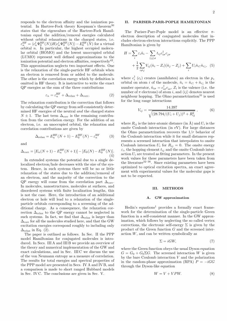
2
responds to the electron affinity and the ionization po-tential. In Hartree-Fock theory Koopman’s theorem30
states that the eigenvalues of the Hartree-Fock Hamil-tonian equal the addition/removal energies calculatedwithout orbital relaxations in the charged states, i.e.εHF
n = 〈c†nΨHF0 (N)|H |c†nΨHF
0 (N)〉−EHF0 (N) for a virtual
orbital n. In particular, the highest occupied molecu-lar orbital (HOMO) and the lowest unoccupied orbital(LUMO) represent well defined approximations to theionization potential and electron affinities, respectively42.This approximation neglects two important effects. Oneis the relaxation of the single-particle HF orbitals whenan electron is removed from or added to the molecule.The other is the correlation energy which by definition isomitted in HF theory. It is instructive to write the exactQP energies as the sum of the three contributions
εn = εHFn + ∆relax + ∆corr, (2)
The relaxation contribution is the correction that followsby calculating the QP energy from self-consistently deter-mined HF energies of the neutral and the charged statesN ± 1. The last term ∆corr is the remaining contribu-tion from the correlation energy. For the addition of anelectron, i.e. an unoccupied orbital, the relaxation andcorrelation contributions are given by
∆relax = EHFn (N + 1)− EHF
0 (N)− εHFn (3)
and
∆corr = [En(N +1)−EHFn (N +1)]− [E0(N)−EHF
0 (N)].(4)
In extended systems the potential due to a single de-localized electron/hole decreases with the size of the sys-tem. Hence, in such systems there will be no or littlerelaxation of the states due to the addition/removal ofan electron, and the majority of the correction to theQP energy will come from the correlation part ∆corr.In molecules, nanostructures, molecules at surfaces, anddisordered systems with finite localization lengths, thisis not the case. Here, the introduction of an additionalelectron or hole will lead to a relaxation of the single-particle orbitals corresponding to a screening of the ad-ditional charge. As a consequence, the relaxation cor-rection ∆relax to the QP energy cannot be neglected insuch systems. In fact, we find that ∆relax is larger than∆corr for all the molecules studied here, and that the GWexcitation energies correspond roughly to including only∆relax in Eq. (2).
The paper is outlined as follows. In Sec. II the PPPmodel Hamiltonian for conjugated molecules is intro-duced. In Secs. III A and III B we provide an overview ofthe theory and numerical implementation of the GW andexact calculations, and in Sec. III C we discuss the useof the von Neumann entropy as a measure of correlation.The results for total energies and spectral properties ofthe PPP model are presented in Secs. IVA and IVB, anda comparison is made to short ranged Hubbard modelsin Sec. IVC. The conclusions are given in Sec. V.
II. PARISER-PARR-POPLE HAMILTONIAN
The Pariser-Parr-Pople model is an effective π-electron description of conjugated molecules that in-cludes electron-electron interactions explicitly. The PPPHamiltonian is given by
H =∑
i
εini −∑
〈ij〉σ
tijc†iσcjσ
+1
2
∑
i6=j
Vij(ni − Zi)(nj − Zj) +∑
i
Uini↑ni↓, (5)
where c†i (ci) creates (annihilates) an electron in the pz
orbital on atom i of the molecule, ni = ni↑ + ni↓ is the
number operator, niσ = c†iσciσ, Zi is the valence (i.e. thenumber of π electrons) of atom i, and 〈ij〉 denotes nearestneighbour hopping. The Ohno parametrization31 is usedfor the long range interactions
Vij =14.397
√
(28.794/(Ui + Uj))2 + R2ij
, (6)
where Rij is the inter-atomic distance (in A) and Ui is theonsite Coulomb interaction (in eV). For large distancesthe Ohno parametrization recovers the 1/r behavior ofthe Coulomb interaction while it for small distances rep-resents a screened interaction that interpolates to onsiteCoulomb interaction Ui for Rij = 0. The onsite energyεi, the hopping element tij and the onsite Coulomb inter-action Ui are treated as fitting parameters. In the presentwork values for these parameters have been taken fromthe literature32–36. Since existing parameters have beenoptimized to optical excitation spectra, an exact agree-ment with experimental values for the molecular gaps isnot to be expected.
III. METHODS
A. GW approximation
Hedin’s equations1 provides a formally exact frame-work for the determination of the single-particle Greenfunction in a self-consistent manner. In the GW approx-imation, which follows by neglecting the so called vertexcorrections, the electronic self-energy Σ is given by theproduct of the Green function G and the screened inter-action W , and can be written symbolically as
Σ = iGW, (7)
where the Green function obeys the usual Dyson equationG = G0 + G0ΣG. The screened interaction W is givenby the bare Coulomb interaction V and the polarizationin the random-phase approximation (RPA) P = −iGGthrough the Dyson-like equation
W = V + V PW. (8)

3
In fully self-consistent GW the set of coupled equationsfor Σ, G, P , and W are solved iteratively until theGreen function has converged. Due to the computa-tional requirement of a fully self-consistent GW scheme,ab-initio GW calculations are usually carried out non-selfconsistently. This approach, which is referred to asG0W0, starts from an approximate G0, typically the non-interacting Kohn-Sham Green function, from which a sin-gle self-energy iteration is carried out to obtain the finalGreen function.
1. Numerical details
The GW calculations have been performed followingthe method described in detail in Ref. 37. Here we givea brief overview of the method for completeness.
The retarded and advanced single-particle Green func-tions are given by
Gr/a(ε) = (ε± iη −H0 − VH − ΣGW (ε))−1 (9)
where η is a small positive infinitesimal, H0 containsthe first two terms in Eq. (5), and VH is the Hartreepotential. We represent the Green functions and allother energy-dependent quantities on a uniform grid,−Em,−Em + dε, . . . , Em. The Fast Fourier Transformis used to switch between the energy and time rep-resentations. Since η determines the minimum widthof features in the Green function’s energy dependence,the energy grid spacing should obey dε ≪ η. All re-sults presented here have been converged with respectto η, dε, Em. Typical converged values are (in eV) η =0.02, dε = 0.005, Em = 50.
The lesser/greater Green functions are given by
G<(ε) = −f(ε− µ)[Gr −Ga] (10)
G>(ε) = (1− f(ε− µ))[Gr −Ga] (11)
where f(ε−µ) is the Fermi-Dirac function. The chemicalpotential µ is adjusted to yield the desired number ofelectrons in the system. The formulation in terms ofa fixed chemical potential rather than a fixed particlenumber is reminiscent of the fact that the method hasbeen developed for quantum transport. The one-bodydensity matrix is given by
ρij = −i
∫
G<ij(ε)dε. (12)
From ρ the Hartree and exchange potentials follow
VH,ij = 2∑
k
Vikρkk) (13)
Vx,ij = −Vijρij , (14)
where we have defined Vii = Ui, see Eq. (5).The retarded/advanced and lesser/greater components
of the quantities needed to construct the GW self-energy
read37
Σ</>GW,ij(t) = iG
</>ij (t)W
</>ij (t) (15)
W</>ij (ε) =
∑
kl
W rik(ε)P
</>kl (ε)W a
lj(ε) (16)
Wr/aij (ε) =
∑
k
Pr/aik [1− V P r/a(ε)]−1
kj (17)
P</>ij (t) = G
</>ij (t)G
>/<ji (−t) (18)
The GW equations have been expressed in the time or en-ergy domain according to where they are simplest. Thisalso reflects the practical implementation.
The retarded components of ΣGW and P are obtainedusing the fundamental relation
F r(t) = −iθ(t)[F>(t)− F<(t)] (19)
which is the Kramers-Kronig relation in the time domainrelating the imaginary and real parts of F r.
Since the GW self-energy depends on the Green func-tion and vice versa, the equations must be iterated untilself-consistency. To speed up converence we use the Pu-lay mixing scheme38 as described in Ref. 37.
2. Total energy
The total energy can be split into kinetic (and ex-ternal), Hartree, and exchange-correlation energy E =E0 + EH + Exc. In terms of the Green function we have
E0 + EH = Tr[H0ρ] +1
2Tr[VHρ] (20)
For the exchange-correlation energy we have
Exc =1
2i
∫
Tr[Σr(ε)G<(ε) + Σ<(ε)Ga(ε)]dε, (21)
where Σ is the exchange-correlation self-energy. In thiswork Σ is either the bare exchange, Σx, yielding the HFapproximation, or the GW self-energy, ΣGW. The expres-sion (21) follows by expressing 〈V 〉 in terms of the two-particle Green function, G2, and then using the definingequation for the self-energy in terms of G2
39.
B. Exact diagonalization
The most direct way to the spectral properties of asystem is via the Lehmann representation of the Greenfunction in Eq. (1). However, since this requires the fullset of eigenstates and eigenvalues of the Hamiltonian,it is of limited practical use and other routes must betaken. The following section gives a brief overview ofthe Lanczos method for iterative diagonalization of largematrices.

4
1. Calculating the ground state - Lanczos algorithm
In exact diagonalization the given many-body Hamil-tonian is diagonalized directly in the Fock space which isspanned by many-particle states (Slater determinants).Since the dimensionality of the Fock space grows expo-nentially with the number of basis orbitals, symmetriesof the Hamiltonian can help to reduce the dimensionalityconsiderably. For the Pariser-Parr-Pople Hamiltonian inEq. (5) the number of up and down electrons, N↑ andN↓, are good quantum numbers since their correspond-ing operators commute with the Hamiltonian. This im-plies that the exact diagonalization can be carried outin each of the (N↑, N↓)-subblocks of the Fock space inde-pendently. The dimensionality of each (N↑, N↓)-subblockis given by the number of ways N↑ spin up electrons andN↓ spin down electrons can be distributed over L basisorbitals,
d(N↑, N↓) =L!
N↑!(L−N↑)!×
L!
N↓!(L−N↓)!. (22)
Very often the ground state is located in the half-filledsubblock, i.e. N↑ = N↓ = L/2 where L is the number ofbasis orbitals. For L = 16 the dimensionality of this sub-block is d = 165636900, implying that storing a vector indouble floating point precision requires ∼ 1 Gb of mem-ory. With such memory requirements a full diagonaliza-tion of the Hamiltonian is of course out of reach. If onlythe ground state is needed, iterative methods can be em-ployed. The basic idea of iterative methods is to projectthe Hamiltonian onto the Krylov subspace K generatedby repeated applications of H on an arbitrary initial state|φ0〉, i.e.
K = span|φ0〉, H |φ0〉, H2|φ0〉, · · · , HN |φ0〉. (23)
In the Krylov subspace the extreme eigenvalues of theHamiltonian converge fast with respect to the size N ofthe subspace, thus reducing the full diagonalization toa manageable diagonalization of a N × N matrix, withN ≪ d.
In the Lanczos algorithm43 the Hamiltonian is pro-jected onto a specially constructed orthogonalised Krylovbasis in which the Hamiltonian has a tridiagonal repre-sentation. The basis vectors are generated recursivelyas
|φn+1〉 = H |φn〉 − an|φn〉 − b2n|φn−1〉, (24)
where the coefficient are given by
an =〈φn|H |φn〉
〈φn|φn〉and b2
n =〈φn|φn〉
〈φn−1|φn−1〉(25)
with initial conditions b0 = 0 and |φ−1〉 = 0. At anypoint during the Lanczos iterations only three Lanczosvectors needs to be kept in memory, which makes the al-gorithm memory efficient. In the basis of the normalized
vectors (the basis vectors above are not normalized) theHamiltonian has the following tridiagonal representation
H =
a0 b1 0 · · · 0
b1 a1 b2
...
0 b2 a2. . . 0
.... . .
. . . bN
0 · · · 0 bN aN
(26)
which can be readily diagonalized with methods for tridi-agonal matrices. In practice the Lanczos iterations arecontinued until the desired eigenvalues have converged toa given tolerance. For the ground state energy E0, typi-cal values for N range from a few to ∼ 200 depending onthe system size.
The ground state resulting from a diagonalization ofthe tridiagonal Hamiltonian in Eq. (26) is provided inthe Lanczos basis, i.e. |Ψ0〉 =
∑
n cn|φn〉. In order to beable to calculate the Green function, its representationin the original many-body basis is required. Since theLanczos vectors are not stored, the Lanczos iterationsmust be repeated (starting from the same initial vector)to obtain the expansion coefficients αi =
∑
n cn〈Φi|φn〉in the original many-body basis |Φi〉
di=1.
The most time consuming part of the Lanczos algo-rithm is the matrix-vector multiplication H |φn〉. An ef-ficient implementation of this part is hence crucial. Forthis purpose it is convenient to use the bit representationof an unsigned integer to code the basis states. Denotingthe integers with bit representations corresponding to thespin up and spin down occupations of a given basis statewith I↑ and I↓, respectively, the integer representation ofthe basis state is I = I↑ + 2LI↓. With the binary rep-resentation of the basis states, the multiplication of theHamiltonian can be done efficiently using bitwise opera-tions.
2. Calculating the Green function
Having obtained the ground state, the Green functioncan now be calculated. From the Lehmann representa-tion it follows that it can be written as
Grij(ε) = Ge
ij(ε) + Ghij(ε) (27)
with the electron and hole Green functions defined by
Geij(ε) = 〈ΨN
0 |ci
1
ε−H + EN0 + iη
c†j |ΨN0 〉 (28)
and
Ghij(ε) = 〈ΨN
0 |c†j
1
ε + H − EN0 + iη
ci |ΨN0 〉, (29)
respectively. In the following we focus on the electronGreen function which is the matrix representation of the
5
resolvent operator (z − H)−1 in the basis spanned by
the |i〉 = c†i |ΨN0 〉 vectors. To obtain the i’th diagonal
element,
Geii(ε) = 〈i|(z −H)−1|i〉, (30)
where z = ε + EN0 + iη, again the Lanczos algorithm is
used to put H on a tridiagonal form, but this time theLanczos iterations are started from the normalized initialstate |φ0〉 = |i〉/b0 where b2
0 = 〈i|i〉. Hence, in the gen-erated Krylov subspace the diagonal element in Eq. (30)corresponds to the matrix element b2
0[(ε − H + EN0 +
iη)−1]11 of a tridiagonal matrix, which can be obtainedas the continued fraction40
Geii(ε) =
b20
ε− a0 −b21
ε− a1 −b22
ε− a2 − · · ·
. (31)
Again the Lanczos iterations are continued until the fre-quency dependent Green function element has converged.
C. Von Neumann entropy
The following section demonstrates how a quantitativemeasure of the degree of correlations in a system can beobtained by considering the von Neumann entropy of thereduced single-particle density matrix ρ. The entropy isdefined by
S[ρ] = −Tr[ρ log ρ] = −∑
n
ρn log ρn, (32)
where in the last equality ρ has been expressed in itsdiagonal representation, ρ =
∑
n ρn|n〉〈n|.In the basis of the atomic pz orbitals the matrix ele-
ments of the reduced density matrix are given by (withthe spin index suppressed)
ρij = 〈Ψ0|c†jci |Ψ0〉, (33)
with the diagonal elements equal to the site occupations.In the diagonal representation ρn thus represents the oc-cupation of the eigenstate |n〉 of the density matrix.
We note that 0 ≤ S ≤ L log 2, where 2L is the di-mension of the single-particle Hilbert space includingspin. The expression for Smax follows because the num-ber of electrons equal L in all the systems, i.e. half filled“band”. When |Ψ0〉 is a single Slater determinant (cor-responding to zero correlation) we have S = 0, and when|Ψ0〉 has equal weight on a complete set of orthogonalSlater determiants (corresponding to maximal correla-tion) we have ρn = 1/2 for all n and thus S = L log 2.Thus the number 0 ≤ S/Smax ≤ 1 represents a naturalmeasure of the degree of correlation in |Ψ0〉.
IV. RESULTS
A. Total energies
We first address the degree of correlation in the ex-act ground states by considering the von Neumann en-tropies of the corresponding density matrices. The cal-culated entropies are listed in Tab. I. Except for theHubbard description of benzene (see Sec. IVC) whichclearly presents strong correlations, the entropies of theground states are ∼ 10% of their maximum value Smax
corresponding to weakly correlated systems. The finitevalues of the entropies reveal that none of the groundstates are single Slater determinants implying that theHartree-Fock ground state energies will be larger thanthe exact ones.
We here follow the usual convention and define thecorrelation energy as the part of the total energy notincluded in Hartree-Fock, i.e.
Ecorr = Eexact − EHF. (34)
Fig. 1 shows the exact correlation energies of the neu-tral molecules together with those obtained by evaluat-ing the total energy from Eqs. (20) and (21) with theself-consistently determined Green function and GW self-energy.
For the series of molecules considered here the correla-tion energy constitute less than 0.5% of the total energies.Furthermore, as expected it decreases (in absolute size)with the number of atoms in the molecule. Clearly, theGW approximation performs reasonably well for all themolecules capturing on average 66% of the correlationenergy.
B. Spectral properties
For isolated systems such as molecules, true quasi-particles resembling single-particle excitations are char-
Formula L S/Smax Egap (eV)
thiophene C4H4S 5 0.07 11.19
pyridine C5H5N 6 0.11 10.61
benzene C6H6 6 0.10 11.39
benzene (Hubbard) - - 0.50 -
biphenyl C12H10 12 0.10 9.24
naphthalene C10H8 10 0.11 8.65
anthracene C14H10 14 0.12 7.06
OPV2 C14H12 14 0.10 8.30
TABLE I: Chemical formula, number of pz orbitals (L) in-cluded in the PPP model and exact ground state entropies(S) for the listed molecules.

6
FIG. 1: (Color online) Exact and GW correlation energies ofthe neutral groundstate of the seven molecules.
acterized by having a weight close to unity (for non-degenerate levels) in the spectral function, i.e.
Zn =∑
i
|〈ΨN+1n |c†i |Ψ
N0 〉|
2 ∼ 1. (35)
This is equivalent to saying that there exists an orbital|ν〉 so that the excited state 〈ΨN+1
n | can be written asthe single-particle excitation c†ν |Ψ
N0 〉. In Fig. 2 we show
the single-particle density of states (DOS),
D(ε) =∑
i
Ai(ε) (36)
for the OPV2 molecule on a logarithmic scale. The heightof the peaks reflects the value of Zn (modulo degenera-cies). The HF and, in particular, the GW approximationreproduce the lowest lying excitations quite well whilehigher excitations are poorly described. All the peaksin the HF spectrum have Zn = 1 while GW does shiftsome spectral weight from the main peaks to tiny satelitestructures (at higher energies than shown on the plot).However, the GW satelites do not correspond to featuresin the exact spectrum. This shows that excitations withZn ≪ 1, i.e. excitations which do not have single-particlecharacter, are not well described by GW whose main ef-fect is to improve the position of the HF single-particlepeaks.
In the following we consider the lowest lying single-particle excitations of the molecules as obtained withHartree-Fock, G0W0 and self-consistent GW. In theG0W0 calculations the starting Green function G0 istaken to be the self-consistently determined Hartree-FockGreen function. Fig. 4 gives an overview of the calculatedexcitation energies relative to the exact ones. Energiescorresponding to electron removal and electron additionare located on the negative and positive half of the x-axis,respectively. From this plot clear trends in the calculatedexcitation energies emerge.
FIG. 2: (Color online) Single-particle DOS of the OPV2molecule. Note the logarithmic axis.
Starting with HF, the occupied (unoccupied) levels aresystematically overestimated (underestimated). The de-viation from the exact values worsens for the higher lyingexcitations.
A close inspection of the figure reveals a few HF en-ergies at ∼ ±5.0 eV and ∼ ±5.7 eV that more or lesscoincide with the exact energies. These are the HOMOand LUMO levels of the small single-ring molecules thio-phene, pyridine and benzene. The good agreement withthe exact levels for these systems is not a result of HFgiving a correct description of the many-body states andtheir energies – this was already clear from the analysisabove which showed that the eigenstates are not singleSlater determinants and hence the excitation energies inEq. (2) have contributions from both ∆relax and ∆corr.The good agreement must therefore be ascribed to can-cellations between the relaxation and correlation contri-bution to the exact energies (this is discussed further inconnection with Fig. 4).
Both the G0W0 and the GW give consistently betterenergies than HF – in particular for the higher lying ex-citations where the absolute errors are reduced to lessthan ∼0.4 eV as compared to ∼1 eV for HF. For the low-lying excitations GW slightly overestimates (underesti-mates) the occupied (unoccupied) levels correspondingto an overcorrection of the HF energies.
In order to address the relative contributions from∆relax and ∆corr to the excitation energies in Eq. (2),we plot in Fig. 4 the difference between the exact gapsand the gaps obtained from the (i) Hartree-Fock eigen-values, (ii) Hartree-Fock total energy differences with
self-consistent relaxations in the N ± 1 Slater deter-minants taken into account, and (iii) the distance be-tween the highest occupied and lowest unoccupied peaksin the GW spectral function. By using the expressionfor the quasi-particle energies in Eq. (2), the exact gap

7
FIG. 3: (Color online) Energy of the 3 highest occupied and3 lowest unoccupied molecular orbitals relative to the exactvalues. While Hartree-Fock underestimates the occupied andoverestimates the unoccupied levels, self-consistent GW showsthe opposite trends but deviates on average less from the exactresult.
Egap = εLUMO − εHOMO can be expressed as
Egap = εHFLUMO − εHF
HOMO + ∆gaprelax + ∆gap
corr (37)
where ∆gaprelax and ∆gap
corr are the gap equivalents of the cor-responding quantities in Eq. (2) and εHF
HOMO/LUMO are
the Hartree-Fock HOMO/LUMO eigenvalues. By defini-tion ∆gap
relax is difference between the gaps obtained fromthe HF eigenvalues and relaxed HF total energy differ-ences. In Fig. 4 this is given by the vertical distancebetween the (blue) squares and circles. The correlationcontribution ∆gap
corr can be read off as the difference be-tween the exact gap (dashed horizontal line) and the re-laxed HF total energy gap (blue squares). Inclusion ofrelaxation effects clearly reduces the HF gaps consider-ably implying that ∆gap
relax < 0. This reduction is due tothe screening from the orbital relaxation which reducesthe Coulomb interaction with the added hole or electronand hence also the gap.
We note that the HF eigenvalues give excellent gapsfor the small single-ring molecules thiophene, pyridineand benzene. The good agreement with the exact lev-els for these systems is not a result of HF giving a cor-rect description of the many-body states and their en-ergies – this was already clear from the analysis abovewhich showed that the eigenstates are not single Slaterdeterminants and hence the excitation energies in Eq. (2)have contributions from both ∆relax and ∆corr. The goodagreement must therefore be ascribed to cancellations be-tween the relaxation and correlation contribution to theexact energies
In contrast to the HF (eigenvalue) gaps for which theagreement with the exact gap worsens as a function of
FIG. 4: (Color online) The HOMO-LUMO gap relative to theexact values. In addition to the HF and GW single-particleenergies, the relaxed Hartree-Fock total energy differences,EHF
0 (N + 1) + EHF0 (N − 1) − 2EHF
0 (N) are also shown. Theexcellent results of HF for the three smallest molecules is aresult of error cancellation between relaxation and correlationcontributions.
the size of the molecules, the GW gaps follow more con-sistently the same trend and underestimates the exactgaps with 0.05− 0.35 eV for all the molecules. The closeresemblance between GW and the relaxed HF result in-dicates that the effect of GW is mainly to account for thescreening effects included in HF via orbital relaxations,∆relax.
C. Long- versus short-range interactions
To demonstrate the shortcomings of the GW approx-imation for strongly correlated systems, we consider aHubbard model description of the benzene molecule. Itshould be noted that this Hubbard description of benzeneis not intended as a realistic description of the benzenemolecule, rather it serves to illustrate the limitations ofthe GW approximation. The Hamiltonian is identical tothe PPP-Hamiltonian in Eq. (5), except that the longrange Coulomb interactions in the third term have beenomitted. The values for the hopping elements and theonsite Coulomb interaction are t = 2.539 and U = 10.06,respectively. With a U/t-ratio of ∼4 this obviously repre-sent a strongly correlated system. The latter is reflectedin the ground state entropy in Tab. I which is 50% of itsmaximum value.
From the calculated total energies we find that the cor-relation energy (not included in Fig. 1) constitutes 10%of the ground state energy which is a considerably higherfraction as for the PPP descriptions of the molecules.The GW total energy captures 88% of the correlationenergy compared to 66% on the average for the PPP de-scriptions. However, from an absolute point of view, the

8
GW approximation misses the exact ground state energyby 0.48 eV. This should be compared to 0.16 eV whichis the difference between the exact and the GW groundstate energy for the PPP description of benzene.
The poor performance of both Hartree-Fock and GWfor the spectral properties of the Hubbard benzene is il-lustrated in Fig. 5 which shows the spectral function ascalculated with the two methods together with the exactone. Both Hartree-Fock and GW severely underestimatesthe position of the LUMO level and completely misses thedetails of the spectrum at higher energies.
This clearly demonstrates that GW is of limited rele-vance when considering systems where correlation effects(∆corr) dominates over screening, or relaxation, effects(∆relax).
FIG. 5: (Color online) Single-particle DOS for the Hubbarddescription of the benzene molecule (only on-site interactionsfrom the PPP model are kept). Note the logarithmic axis.
V. CONCLUSION
We have presented calculations for the total energyand charged single-paticle excitations in seven conju-gated molecules described by the semi-empirical PPPmodel within fully self-consistent GW and exact diago-nalization. The results show that the GW approximationgives a consistently good description of both total ener-gies and electronic excitations with a slight tendency tooverestimate (underestimate) the position of the latterfor occupied (unoccupied) levels. We have found thatthe effect of the GW self-energy is similar to the inclu-sion of orbital relaxations in the N ± 1 final states inHartree-Fock theory. On the other hand the contribu-tion to the excitation energies coming from correlationsin the ground- and excited states is less well describedby GW. This explains why GW tend to reduce electronaddition/removal energies relative to the HF eigenval-ues. Finally, we showed that GW does not perform wellfor systems with short range interactions (Hubbard mod-els) where correlation effects are dominating over screen-ing/relaxation effects.
VI. ACKNOWLEDGEMENTS
Financial support from the Danish Council for Pro-duction and Technology (FTP) under Grant 26-04-0181“Atomic scale modeling of emerging electronic devices”is acknowledged. KST acknowledges support from theDanish Center for Scientific Computing. The Center forAtomic-scale Materials Design (CAMD) is sponsored bythe Lundbeck Foundation.
1 L. Hedin, Phys. Rev. 139, A796 (1965).2 M. S. Hybertsen and S. G. Louie, Phys. Rev. B 34, 5390
(1986).3 W. G. Aulbur, L. Jonsson, and J. W. Wilkins, in Solid
State Physics, edited by H. Ehrenreich and F. Saepen (Aca-demic Press, New York, 2000), vol. 54, p. 1.
4 F. Aryasetiawan and O. Gunnarsson, Rep. Prog. Phys. 61,237 (1998).
5 G. Onida, L. Reining, and A. Rubio, Rev. Mod. Phys. 74,601 (2002).
6 J. C. Grossman, M. Rohlfing, L. Mitas, S. G. Louie, andM. L. Cohen, Phys. Rev. Lett. 86, 472 (2001).
7 A. Stan, N. E. Dahlen, and R. van Leeuwen, Europhys.Lett. 76, 298 (2006).
8 C. D. Spataru, S. Ismail-Beigi, X. L. Benedict, and S. G.Louie, Phys. Rev. Lett. 92, 077402 (2004).
9 P. E. Trevisanutto, C. Giorgetti, L. Reining, M. Ladisa,and V. Olevano, Phys. Rev. Lett. 101, 226405 (2008).
10 M. L. Tiago and J. R. Chelikowsky, Phys. Rev. B 73,205334 (2006).
11 J. B. Neaton, M. S. Hybertsen, and S. G. Louie, Phys.
Rev. Lett. 97, 216405 (2006).12 C. Freysoldt, P. Rinke, and M. Scheffler, Phys. Rev. Lett.
103, 056803 (2009).13 K. Kaasbjerg and K. Flensberg, Nano. Lett. 8, 3809
(2008).14 K. S. Thygesen and A. Rubio, Phys. Rev. Lett. 102,
046802 (2009).15 C. D. Spataru, L. X. Benedict, and S. G. Louie, Phys. Rev.
B 69, 205204 (2004).16 K. S. Thygesen and A. Rubio, J. Chem. Phys. 126, 091101
(2007).17 P. Darancet, A. Ferretti, D. Mayou, and V. Olevano, Phys.
Rev. B 75, 075102 (2007).18 K. S. Thygesen, Phys. Rev. Lett. 100, 166804 (2008).19 P. Myohanen, A. Stan, G. Stefanucci, and R. van Leeuwen,
Europhys. Lett. 84, 67001 (2008).20 C. D. Spataru, M. S. Hybertsen, S. G. Louie, and A. J.
Millis, Phys. Rev. B 79, 155110 (2009).21 M. P. von Friesen, C. Verdozzi, and C.-O. Almbladh,
arXiv:0905.2061 (2009).22 N. E. Dahlen and R. van Leeuwen, Phys. Rev. Lett. 98,

9
153004 (2007).23 J. A. Pople, Trans. Faraday Soc. 49, 1375 (1953).24 R. Pariser and R. G. Parr, J. Chem. Phys. 21, 466 (1953).25 R. Pariser and R. G. Parr, J. Chem. Phys. 21, 767 (1953).26 A. Schindlmayr, T. J. Pollehn, and R. W. Godby, Phys.
Rev. B 58, 12684 (1998).27 T. J. Pollehn, A. Schindlmayr, and R. W. Godby, J. Phys.:
Condens. Matter 10, 1273 (1998).28 C. Verdozzi, R. W. Godby, and S. Holloway, Phys. Rev.
Lett. 74, 2327 (1995).29 C. Rostgaard, K. W. Jacobsen, and K. S. Thygesen, sub-
mitted30 P. Fulde, Electron Correlations in Molecules and Solids,
no. 100 in Springer Series in Solid-State Sciences (Springer,Berlin, 1995), 3rd ed.
31 K. Ohno, Theor. Chim. Acc. 2, 219 (1964).32 I. R. Ducasse, T. E. Miller, and Z. G. Soos, J. Chem. Phys.
76, 4094 (1982).33 W. Barford and R. J. Bursill, Chem. Phys. Lett. 268, 535
(1997).34 R. J. Bursill, C. Castleton, and W. Barford, Chem. Phys.
Lett. 294, 305 (1998).35 W. Barford, R. J. Bursill, and M. Y. Lavrentiev, J. Phys.:
Condens. Matter 10, 6429 (1998).36 M. Y. Lavrentiev, W. Barford, S. J. Martin, and H. Daly,
Phys. Rev. B 59, 9987 (1999).37 K. S. Thygesen and A. Rubio, Phys. Rev. B 77, 115333
(2008).38 P. Pulay, Chem. Phys. Lett. 73, 393 (1980).39 A. L. Fetter and J. D. Walecka, Quantum theory of many-
particle systems (McGraw-Hill, New York, 1971).40 E. Dagotto, Rev. Mod. Phys. 66, 763 (1994).41 P. Dayal, M. Troyer, and R. Villiger, The Iterative Eigen-
solver Template Library (IETL), http://www.comp-phys.org/software/ietl/.
42 In the remaining of the paper HOMO and LUMO abbrevi-ations will be used to refer to the ionization potential andelectron affinity also outside Hartree-Fock theory.
43 The present work has used the implementation from theIETL project41.