Single image shadow removal by optimization using non

Computational Visual Mediahttps://doi.org/10.1007/s41095-019-0148-x Vol. 5, No. 3, September 2019, 311–324

Research Article

Single image shadow removal by optimization using non-shadowanchor values

Saritha Murali1 (�), V. K. Govindan1, and Saidalavi Kalady1

c© The Author(s) 2019.

Abstract Shadow removal has evolved as a pre-processing step for various computer vision tasks.Several studies have been carried out over the pasttwo decades to eliminate shadows from videos andimages. Accurate shadow detection is an open problembecause it is often considered difficult to interpretwhether the darkness of a surface is contributed by ashadow incident on it or not. This paper introducesa color-model based technique to remove shadowsfrom images. We formulate shadow removal as anoptimization problem that minimizes the dissimilaritiesbetween a shadow area and its non-shadow counterpart.To achieve this, we map each shadow region to a setof non-shadow pixels, and compute an anchor valuefrom the non-shadow pixels. The shadow region is thenmodified using a factor computed from the anchor valueusing particle swarm optimization. We demonstrate theefficiency of our technique on indoor shadows, outdoorshadows, soft shadows, and document shadows, bothqualitatively and quantitatively.

Keywords mean-shift segmentation; particle swarmoptimization; HSV; YCbCr; anchorvalues

1 IntroductionShadowing is a physical phenomenon arising in areasof a surface where the illumination is lower thanadjacent areas due to an obstructing opaque objectpresent between the surface and the light source.The geometry and density of shadows vary dependingon the number and position of light sources, the

1 Department of Computer Science and Engineering,National Institute of Technology Calicut, Kerala 673601,India. E-mail: S. Murali, [email protected] (�); V.K. Govindan, [email protected]; S. Kalady, [email protected].

Manuscript received: 2019-01-29; accepted: 2019-05-18

geometry of the obstructing object, and the distancebetween the object and the surface. For instance, atdifferent time of day, the shadow cast by the Sunon the ground changes dramatically depending onthe elevation angle between the Sun and the horizon.Shadows are shorter at noon when the elevation angleis large, and are larger early or late in the day whenthe elevation angle is small.The presence of shadows in images and videos

reduces the success rate of machine vision applicationssuch as edge extraction, object identification, objectcounting, and image matching. Some scenariosin which shadows affect different applicationsare demonstrated in Fig. 1. Image segmentationtechniques may incorrectly classify a shadow regionas an object or as a portion of an object. Thismisclassification may in turn affect the detectionof objects, as shown in Fig. 1(a) where the part ofthe pavement in shadow is misclassified as a portionof the brick seat. Shadows may also cause objectmerging in video tracking systems. Figure 1(b)illustrates a case in which two vehicles are mergedand counted as a single object due to the connectingshadow region. Shadows can also obstruct imageinterpretation in remote-sensing images, and thusprevent target detection (e.g., locating roads), asdemonstrated in Fig. 1(c). The challenge posed byillumination inconsistencies, especially shadows, inthe lane detection module of driver assistance systemsis mentioned in Ref. [1].Based on their density (i.e., darkness), shadows can

be classified into hard shadows and soft shadows. Asthe name indicates, hard shadows have high density,and the surface texture is nearly destroyed. On theother hand, soft shadows have low density, and theirboundaries are usually diffused to the non-shadowsurroundings. Furthermore, the shadow generated by

311

312 S. Murali, V. K. Govindan, S. Kalady

Fig. 1 Shadows causing problems in (a) object detection, (b) traffic monitoring, and (c) interpretation of remote-sensing images.

obstruction of a non-point light source by an objecthas two distinct regions, the umbra and penumbra.The umbra is the high density region, lying towardsthe inner shadow area, while the penumbra is the lowdensity region, lying towards the outer shadow area.Each of these shadow areas is depicted in Fig. 2.Over the past two decades, numerous studies have

been conducted on the detection and removal ofshadows appearing in images [2, 3] and videos [4].Shadow elimination from a single image is morechallenging since the only source of informationavailable is that single image, and there is nocontext. Removal of shadows is often consideredto be a relighting task in which the brightness ofshadow pixels is increased to make them as wellilluminated as the non-shadow surroundings. In thesurvey [5], shadow removal techniques are categorizedinto reintegration methods [6], relighting methods[7], patch-based methods [8], and color transfermethods [9]. Furthermore, these techniques areeither automatic [7] or interactive [10], dependingon whether the user is provided an interface toincorporate his knowledge into the system. Variousworks related to shadow removal are presented in thenext section.

The rest of this paper is structured as follows. Aconcise view of the state-of-the-art shadow removaltechniques is presented in Section 2. Section 3 brieflydiscusses background information related to theproposed work. Section 4 details our proposed shadowelimination framework. Experimental results andcomparison with other shadow removal algorithmsare included in Section 5. Section 6 discussesapplications and limitations of the proposed method,and Section 7 concludes the paper with someobservations on possible future enhancements to theproposed method.

2 Previous work

Several methods are available for shadow eliminationfrom indoor images, natural images, satellite images,and videos. Early works on shadow removal froman image are based on the assumption that cameracalibration is necessary to generate a shadow-freerepresentation, called an invariant image. Finlaysonet al. [6] introduced a method to develop ashadow invariant by projecting the 2D chromaticityperpendicular to the illumination-varying direction.Another way to construct the invariant image is

Fig. 2 Types of shadow: (a) hard shadow, (b) soft shadow, (c) shadow regions, umbra and penumbra.

Single image shadow removal by optimization using non-shadow anchor values 313

by minimizing entropy [11], which does not needcalibrated cameras. Shadow edges are determinedusing edge detection on both original and invariantimages. Image gradient along the shadow edges isthen replaced by zeroes, followed by integration togenerate the shadow-free image. These techniquesrequire high-quality input images; however. Yanget al. [12] derived a 3D illumination invariant imagefrom a 2D illumination invariant image and jointbilateral filtering. The detail layer from this 3Dillumination invariant image is then transferred tothe input shadow image to obtain the shadow-freeimage.Baba et al. [13] used brightness information to

segment an image into lit, umbra, and penumbraregions. Shadow regions are modified by adjustingthe brightness and color. This method applies only toimages of single textures. Features that differentiateshadow regions from their non-shadow counterpartsare used for shadow detection in monochromaticimages by Zhu et al. [14]. A classifier trainedusing features such as intensity, local maximum,smoothness, skewness, gradient and texture measures,entropy, and edge response is used for shadowidentification. In Ref. [15], monochromatic shadowsare corrected in the gradient domain by fitting aGaussian function for each vertical and horizontalline segment across the shadow boundary. Arbel andHel-Or [16] showed that shadows could be clearedby adding them to a constant value in log space.Guo et al. [7] also used a scaling constant to relightshadow pixels. They used a region-based techniqueto detect shadows in natural images. A single-region classifier and a pairwise classifier are trainedusing support vector machines (SVMs). An energyfunction combining these classifier predictions is thenminimized using graph cut. Such region-based shadowremoval is shown to provide better results than pixel-based methods. In Ref. [8], the best matching shadowmatte is estimated for each shadow patch using aMarkov random field. This matte is separated fromthe image, leading to a shadow-free output. Thetechnique proposed by Sasi and Govindan [17] splitsand merges adjacent homogeneous quadtree blocksin the image based on a fuzzy predicate built usingentropy, edge response, standard deviation, and meanof quadtree blocks.Interactive shadow detection techniques allow users

to incorporate their knowledge into the detectiontask. The inputs may be a quad map [9], or roughstrokes [18]. The work proposed by Gong and Cosker[10] requires rough scribbles in the shadow andnon-shadow regions. They unwrap the penumbraboundary and perform multi-scale smoothing toderive shadow scales. A recent method by Yu etal. [19] requires the user to provide strokes on theshadow and non-shadow regions. The shadow scalesare estimated using statistics of shadow-free regions,followed by illumination optimization. Certaintechniques use color models which can separateillumination and reflectance components of theimage, such as normalized RGB, c1c2c3, CIE L∗a∗b∗,and HSV to detect shadows [20]. Detection usingthese methods mostly leads to false labeling since apixel is classified as shadow or non-shadow withoutconsidering the neighbors.Vicente et al. [21] mapped each shadow region

to the corresponding lit region using a trainedprobabilistic SVM classifier. Each shadow regionis then enhanced by matching the histogram of theshadow region with the lit region. Recent techniquesfor shadow detection use deep learning to learnshadow features automatically. Khan et al. [22]used deep learning for local and across-boundaryfeatures using two convolutional deep neural networks(CNNs). The most significant structural featuresof shadow boundaries are learned using a CNN inRef. [23]. Although the accuracy of shadow detectionusing feature learning is better than for non-learningapproaches, the time and memory requirements fortraining the classifier are usually high. Shadowremoval results may show more noise in recoveredareas than surrounding non-shadow areas. In suchcases, noise removal [24] is introduced as a post-processing step to provide a seamless transitionbetween shadow and lit areas.This paper presents a simple, color-model based

technique to remove shadows from an image. Shadowremoval is modeled as an optimization task. Everypixel in a shadow segment is modified based on ananchor value computed from a set of non-shadowpixels mapped to the segment. In this way, eachshadow segment is processed to acquire the finalshadow-free image. The method is suitable for bothhard shadows and soft shadows. Also, it recoversthe umbra and penumbra regions by finding different


scale factors for these regions, and there is no needfor a separate method to classify shadow pixels toumbra pixels or penumbra pixels.The next section briefly introduces the color

spaces used in the proposed method, the mean-shift segmentation algorithm, and the particle swarmoptimization (PSO) technique.

3 Background3.1 Color spacesShadow regions are usually darker than theirsurroundings. Therefore, the creation of shadowsis often attributed to the change in illumination. InRGB color space, a pixel is represented using itsintensity in three different color channels, red, green,and blue, whereas in YCbCr color space, a pixelis represented in terms of its brightness and twocolor-difference values. To extract the illuminationinformation from the color information, we transformthe RGB image into YCbCr color space. The Ychannel in YCbCr is the illumination, Cb is the bluedifference, and Cr is the red difference.In order to map shadow regions to non-shadow

regions, we use HSV (hue, saturation, and value)color space. For any pixel, hue represents the basiccolor of the pixel, saturation represents the grayness,and value represents the brightness. Since hue isunaffected by changes in illumination, we assume thatshadows, which are caused by changes in illumination,do not alter the hues of pixels.

3.2 Mean-shift segmentationOur shadow removal system requires the input shadowimage to be segmented into constituent regions. Forthis purpose, we use a non-parametric clusteringtechnique called mean-shift clustering, introduced byFukunaga and Hostetler [25]. In this, we cluster pixelsin RGB space. Pixels with similar colors in RGB colorspace are gathered into the same cluster. Pixels arerecolored according to their cluster, resulting in thesegmented image.The mean-shift method models feature points using

a probability density function where local maxima ormodes correspond to dense areas. Gradient ascentis performed on the estimated density of each datapoint until the algorithm converges. All data pointsbelonging to a particular stationary point are groupedinto a single cluster. The mean-shift algorithm can

be summarized as follows:• For each sample ti, find the mean-shift vector

M(ti).• Shift the density estimation window from ti to

ti +M(ti).• Repeat until the samples reach equilibrium (i.e.,convergence).We use the Edge Detection and Image

Segmentation System (EDISON) developed inthe Robust Image Understanding Laboratory atRutgers University [26–28] to perform mean-shiftsegmentation.

3.3 Particle swarm optimizationIn our work, the removal of shadows is achievedby solving an optimization problem. The objectiveof this optimization problem is to maximize thesimilarity between a shadow area and its non-shadowcounterpart. It is solved using particle swarm opti-mization (PSO) [29]. PSO was developed to modelthe social behavior of an animal in its group, forinstance, the movement of each bird within a flock.The algorithm starts with a group of possible solutionscalled particles and moves these particles in the spacebased on their velocity and position. The position of aparticle depends on the best position of the individualparticle, and of the group. This is repeated until asolution is obtained.

4 Shadow removal by optimizationThe central objective of shadow removal techniquesis to achieve a seamless transition between theshadow and its surroundings by reducing thedifference in intensities of the shadow area andits surroundings. Our novel approach to removingshadows by minimizing this difference is detailed inthis section. Figure 3 depicts the workflow of theproposed method for shadow removal. The input toour system is a color image containing shadowedas well as non-shadowed areas. Shadow regionsare detected using the method in Ref. [7]. Imagesegmentation is done using mean-shift segmentation[27], and each segment is given a unique segmentidentifier (SID).Our shadow removal algorithm is divided into

four stages: (i) decomposition of the image intoframeworks, (ii) initial shadow enhancement, (iii)shadow to non-shadow mapping, and (iv) shadow


Fig. 3 Overall workflow of our proposed shadow removal framework: (a) input shadow image, (b) input image in YCbCr space, (c) mean-shiftsegmentation of input image, (d) image decomposed into frameworks, (e) binary shadow mask with shadow regions in white, (f) shadowsegments mapped to non-shadow regions, (g) YCbCr image after shadow removal, and (h) final shadow-free output in RGB space.

correction. Each of these steps is detailed in thesubsections that follow.

4.1 Splitting the image into frameworksBarrow and Tenenbaum [30] proposed that theformation of any Lambertian image (I) can bemodeled using:

I = R ◦ L (1)

I is the Hadamard product (◦) of the reflectancecomponent (R) and the illumination component (L).Since shadows occur in less illuminated areas, wesegment the image into different frameworks basedon the pixel illumination, so that each frameworkcontains pixels with similar illumination. Forinstance, pixels belonging to hard shadow on asurface would constitute a framework. The concept ofsplitting the image into frameworks is adopted fromthe tone-mapping method for high dynamic range(HDR) images proposed in Ref. [31].Initially, the log10 of the input image illumination

is clustered using the k-means algorithm. For thispurpose, the centroids are initialized to values startingfrom the lowest to the highest illumination of theintensity image with a step size of ten units. The

final set of centroids obtained after convergence ofthe algorithm represents the frameworks. Theseframeworks are further refined by discarding thecentroids with zero pixel membership. To restrictdistinct frameworks with very close illumination,centroid pairs with a difference of less than 0.05 areiteratively merged. If Ci and Ci+1 are two adjacentcentroids to be merged, with Ni and Ni+1 pixelsin each respectively, the new centroid value Cj onmerging Ci and Ci+1 is given by

Cj =CiNi + Ci+1Ni+1

Ni +Ni+1(2)

For a pixel at position i, the probability of itsmembership of each framework is computed as theGaussian of the difference of pixel illumination (Yi)and the centroid representing the framework (Cj). Apixel is classified into the framework for which itsprobability is maximum. Let Fi denote the frameworkto which the ith pixel belongs. Then the probabilityof the ith pixel belonging to the jth framework isgiven by

Pr{Fi = j} = e−(Cj−Yi)2/2σ2(3)

where σ denotes the maximum distance between anytwo adjacent centroids. Frameworks that contain


no pixels with a probability greater than 0.3 areremoved by combining them with adjacent frame-works. Finally, the framework to which each pixelbelongs is recomputed as mentioned above.

4.2 Initial shadow correctionAn initial enhancement of the shadow regions isperformed as a pre-processing step to aid the shadowto non-shadow mapping done in the next phase ofour algorithm. In this step, the shadow regions areroughly enhanced to make them better match the non-shadow equivalents. At first, unwanted texture detailsare removed by applying a mean filter of window size11 × 11 to the input shadow image. Further, eachshadow pixel is enhanced by using a factor computedfrom the pixels constituting the dominant framework(the one with the most pixels). Let P indicate thepixels belonging to this framework, and RP , GP , andBP indicate the mean values of these pixels in eachcolor plane in the filtered image Z. Let X denote thecolor plane for which the mean value is the lowest.Then the factor f is computed as

f = 2− ZshadowX

min(RP , GP , BP )(4)

Shadow pixels are then modified using:Zshadow = f · Zshadow (5)

The output image from this stage is used formapping shadow regions to corresponding non-

shadow regions in the next step.

4.3 Shadow to non-shadow mappingThe objective of this step is to find the matchingset of non-shadow pixels for each shadow segment.An image can contain several disconnected shadowregions, and a single shadow region can containmultiple segments in the segmentation result. LetSIDS and SIDN indicate the segment IDs ofall shadow pixels, and the segment IDs of allnon-shadow pixels, respectively. Each shadowsegment (unique(SIDS)) is processed separately inour method. For this purpose, the image obtainedfrom the initial shadow correction in the previousstage is converted into HSV color space. The shadowsegments are mapped to a set of non-shadow pixelsbased on hue-matching. The hue-matching procedureis described in Algorithm 1.

4.4 Shadow removalOnce the shadow to non-shadow mappings areavailable, shadow removal is done by modifying theY, Cb, and Cr planes of the input image. For eachmapping, we select the framework to which the mostnon-shadow pixels in this mapping belongs. Allnon-shadow pixels in this framework are selectedas candidate pixels. This is followed by computationof an anchor value (A) from the candidate pixels byselecting the highest intensity value after discarding

Algorithm 1 Hue-matching for shadow to non-shadow mappingInput: initial shadow-corrected image in HSV, segmented imageOutput: shadow to non-shadow mapping

1: Cluster the pixels of HSV image into 37 bins of equal width (Bi(i = 1, . . . , 37)) based on their hue values (0 to 360).Bi = Bi

S ∪ BiN (6)

Here, BiS: shadow pixels in Bi, and Bi

N: non-shadow pixels in Bi. Bi, BiS, and Bi

N can be ∅.2: for each y ∈ unique(SIDS) do3: Sort the bins in descending order of number of shadow pixels with SID = y in each bin, i.e., n(y, SID(Bi

S))4: repeat5: Select a bin Bi from the sorted list.6: Compute a weight Wx for each x ∈ unique(SID(Bi

N)).Wx = n(x, SID(Bi

N)) + n(x, SID(surrS)); (7)n(x, SID(Bi

N)) : number of non-shadow pixels with SID = x in bin Bi;n(x, SID(surrS)) : number of non-shadow pixels with SID = x in a dilated neighborhood of shadow segmentS.

7: Sort the weights in descending order.8: Iteratively add the non-shadow pixels belonging to the segment with maximum weights into the set Ny until

the number of selected non-shadow pixels is at least 10% the size of the shadow segment.9: until n(Ny) � 0.1 · n(y, SIDS)

10: end for11: Ny is the final mapped set of non-shadow pixels for each shadow segment y.


the top 5% intensities in each plane [32]. In thisway, separate anchor values are computed for the Y,Cb, and Cr planes. These anchor values are the non-shadow intensities to which the shadow intensitiescan be related. The shadow pixels in each segmentare modified in the Y, Cb, and Cr planes as follows:

Inewi = Iold

i +A

Ioldi

M (8)

where Ioldi and Inew

i indicate the old and modifiedvalue of the ith shadow pixel, respectively. M

is a scale factor computed using particle swarmoptimization by minimizing the deviation of eachshadow pixel from the mean candidate pixel value,subject to the following constraints:

|μc − μs| � 0 (9)

|σc − σs| � 0.4 (10)where s and c indicate the shadow segment andthe mapped set of candidate pixels, respectively.The threshold of 0.4 for Eq. (10) was computed byincluding all images present in the dataset given byGuo et al. [7]. These constraints ensure that shadowsegments are modified such that their mean valuesbecome closer to those of the non-shadow regions. Atthis stage, certain pixels, particularly those near theshadow boundary, may be over-corrected. To addressthis issue, the shadow pixels for which the modifiedvalue exceeds the anchor value in the illuminationplane are considered as a separate segment and areprocessed separately. The modified image in log spaceis finally converted into intensity space, and then toRGB.

5 Experimental resultsThis section present results of our shadow removaltechnique and a comparison with some of theavailable methods for shadow removal from images.Implementation of the algorithm and all theexperimentation was done in MATLAB R2017a on anIntel Core i5-4570 CPU @ 3.20 GHz with 8 GB RAM.For evaluation, the 76 images from the UIUC dataset[7] were divided into two classes based on the methodused by the authors to generate the shadowlessground truth images. Set A consists of 46 images forwhich the ground truth is created by removing theobject causing shadow. Set B consists of 30 imagesfor which the ground truth is captured by removingthe light source responsible for the appearance of

shadow. We also evaluated the performance of theproposed shadow removal method on images fromthe ISTD [33] and LRSS datasets [8].

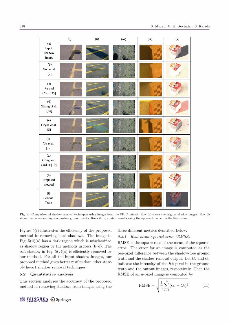
5.1 Qualitative analysisTo illustrate the visual quality of the output of theproposed method, various examples are included inFig. 4 and Fig. 5. The figures also include the outputsobtained using other shadow removal methods. InFig. 4, the results displayed are for five images fromthe UIUC dataset; the first three images are fromSet A, and the next two images are from Set B.For each example, the input shadow image and thecorresponding shadow-free ground truth are includedin rows (a) and (i), respectively. The shadow regionof the input image in Fig. 4(i)(a) has two differentsegments—one with a yellow background, and theother with a gray background. Most existing methodsfail to handle the individual shadow segments, whichis clear from the images in Figs. 4(i)(c–f). Ourproposed method handles each shadow segmentseparately, and the result is better than those ofother methods. Figure 4(ii) also illustrates a similarcase. Guo et al. [7] and Yu et al. [19] were unableto handle the shadow on the yellow lines. Zhanget al. [34] and Gryka et al. [8] failed to remove theshadow. The outputs obtained by Su and Chen [35]and Gong and Cosker [10] have artifacts near thelower region of the shadow.Although the results in Fig. 4(iii) appear to be

good for most of the methods, several visual artifactscan be seen on close observation. Figure 4(iv)(b)demonstrates the scenario in which dark regions inan object are misclassified as shadows by Guo etal. [7], resulting in undesirable modification of thesenon-shadow regions. Gryka et al. [8] was unable topresent a visually pleasing result for the same image.Even though the shadow appears to be removed in theimage in Fig. 4(v)(b), the text on the box is lost. Also,the attempt to remove shadows using Ref. [34] resultsin the false coloring of the shadow region, as shownin Fig. 4(v)(d). The shadow-removal results of thestate-of-the-art methods and the proposed methodfor the 76 images in the UIUC dataset are includedin the Electronic Supplementary Material (ESM).Figure 5 compares the shadow removal results of

various methods on 450 images from the ISTD dataset.Row (a) shows the input shadow images, while row (f)shows the corresponding shadow-free ground truths.


Fig. 4 Comparison of shadow removal techniques using images from the UIUC dataset. Row (a) shows the original shadow images. Row (i)shows the corresponding shadow-free ground truths. Rows (b–h) contain results using the approach named in the first column.

Figure 5(i) illustrates the efficiency of the proposedmethod in removing hard shadows. The image inFig. 5(ii)(a) has a dark region which is misclassifiedas shadow region by the methods in rows (b–d). Thesoft shadow in Fig. 5(v)(a) is efficiently removed byour method. For all the input shadow images, ourproposed method gives better results than other state-of-the-art shadow removal techniques.

5.2 Quantitative analysisThis section analyzes the accuracy of the proposedmethod in removing shadows from images using the

three different metrics described below.5.2.1 Root mean-squared error (RMSE)RMSE is the square root of the mean of the squarederror. The error for an image is computed as theper-pixel difference between the shadow-free groundtruth and the shadow removal output. Let Gi and Oi

indicate the intensity of the ith pixel in the groundtruth and the output images, respectively. Then theRMSE of an n-pixel image is computed by

RMSE =

√√√√ 1n

n∑

i=1(Gi − Oi)2 (11)


Fig. 5 Comparison of shadow removal techniques using images from the ISTD dataset. Row (a) has the original shadow images. Row (f) hasthe corresponding shadow-free ground truths. Rows (b–e) contain results using the approach named in the first column.

Since RMSE is an error measure, a lower valueindicates that the output image is more similar tothe ground truth.5.2.2 Peak signal to noise ratio (PSNR)PSNR is used to find peak error. It computes the peakvalue of SNR, in decibels, between two images. Thevalue of PSNR ranges between 0 and infinity. A higherPSNR value signifies better quality of the outputimage. Initially, we compute the mean-squared error(MSE) between the shadow-free ground truth and theshadow removal output as below:

MSE =1n

n∑

i=1(Gi − Oi)2 (12)

where Gi and Oi indicate the intensity of the ith pixelin the ground truth and output images, respectively.Then the PSNR is computed using:

PSNR = 10 log(η2

MSE) (13)

where η denotes the maximum possible pixel value inthe images.

5.2.3 Structural similarity index (SSIM)SSIM is a metric used to compute the correlationbetween two images. It is considered to be a measurethat is closest to the human visual system. The SSIMformula given in Eq. (14) is a weighted combinationof comparisons of three elements between the images,namely luminance, contrast, and structure:

SSIM(G, O) =(2μGμO + c1)(2σGO + c2)

(μ2G + μ2

O + c1)(σ2G + σ2

O + c2)(14)

where G and O are the shadow-free ground truth andthe shadow removal output, respectively, μG and μO

are the mean values of G and O, σ2G and σ2

O are thevariances of G and O, and σGO is the covariance ofG and O. c1 and c2 are variables computed using thedynamic range of pixels.The average values of RMSE, PSNR, and SSIM

for the two sets of images in the UIUC dataset aretabulated in Table 1. We have computed separateRMSE for shadow areas, non-shadow areas, and


the entire image. The average values of RMSE,PSNR, and SSIM of the original shadow imagewith the corresponding ground truths are includedin the first row of each table. Imperfect shadowdetection has resulted in non-zero RMSE in the non-shadow regions of the original shadow images andthe corresponding ground truths. Another reasonfor this is the misalignment of the input images andthe ground truths. Variations may also arise due tochanges in the direct and ambient light reaching thenon-shadow surface on removal of the shadow source.The values in Table 1 indicate that our results aresuperior to those of other methods.The reason for partitioning the images in the UIUC

dataset into Set A and Set B can be explained bycomparing the first rows in Table 1(a) and Table 1(b).The shadow-free ground truths for Set B images aredarker than their corresponding shadow images sincethese ground truths are generated by eliminating the

light sources causing the shadow (e.g., see Fig. 4(v)).Hence, the shadow region of the ground truth is moresimilar to the shadow region of the original imagethan the results of various shadow removal techniques.This explains the lower shadow region RMSE, andthe higher non-shadow region RMSE of images in SetB for the original shadow images. This reason alsoexplains the higher PSNR and SSIM values.Quantitative results on 450 images from the ISTD

dataset [33] are included in Table 2. The values in thetable indicate that the proposed method performsbetter than other state-of-the-art shadow removaltechniques.Also, to analyze the effectiveness of our shadow

removal approach, we conducted experiments onimages with soft shadows. A method to remove softshadows from images was proposed in Ref. [8]. Aquantitative analysis done on 15 images from theirdataset is included in Table 3. The shadow-free

Table 1 Quantitative results on the images from the UIUC dataset [7]. (a) Images for which the ground truth is created by removing theobject causing shadow. (b) Images for which the ground truth is created by removing the light source responsible for the appearance of theshadow. Values are averages computed over the set of images

(a) 46 images (Set A) in UIUC dataset [7]Method All region RMSE Shadow RMSE Non-shadow RMSE PSNR SSIM

Original shadow image 8.8173 17.3812 2.8577 17.7652 0.9030Su and Chen [35] 4.9956 6.1427 4.5471 22.7521 0.9692Guo et al. [7] 4.7058 6.5041 3.4174 24.7683 0.9694Zhang et al. [34] 4.8693 6.6691 4.1972 23.9528 0.9678Gong and Cosker [10] 4.1367 5.9933 3.0721 25.2210 0.9769Gong and Cosker [18] 4.1087 5.2053 3.5888 25.4569 0.9775Yu et al. [19] 4.6588 5.9763 3.9566 24.5882 0.9730Proposed method 4.0399 5.1585 2.9574 25.6460 0.9871

(b) 30 images (Set B) in UIUC dataset [7]Method All region RMSE Shadow RMSE Non-shadow RMSE PSNR SSIM

Original shadow image 13.8101 3.1606 16.3750 14.4300 0.7512Su and Chen [35] 18.7457 15.0770 19.8418 11.6994 0.6342Guo et al. [7] 16.3436 12.5870 17.8478 13.0993 0.6857Zhang et al. [34] 18.1892 16.9061 18.4132 12.0023 0.6363Gong and Cosker [10] 15.9808 13.1515 16.8974 13.2526 0.6845Gong and Cosker [18] 16.0947 13.4348 17.1333 13.2527 0.6832Yu et al. [19] 16.8660 15.9963 17.2683 12.8850 0.6692Proposed method 16.1408 11.9644 16.5986 13.2843 0.6859

Table 2 Quantitative results for 450 images from the ISTD dataset [33]. The values are averages computed over the set of images

Method All region RMSE Shadow RMSE Non-shadow RMSE PSNR SSIMOriginal shadow image 6.1766 13.7189 3.4580 6.5062 0.9518Yang et al. [12] 7.2868 7.7342 7.1477 6.5163 0.9438Yu et al. [19] 4.9312 5.9729 4.6248 5.9612 0.9710Wang et al. [33] 3.3029 3.7225 3.1293 6.6833 0.9832Proposed method 3.0317 3.2869 3.0466 7.0744 0.9859


Table 3 Quantitative results on 15 images from the soft shadows dataset given by Gryka et al. [8]. The values are averages computed on theset of images

Method All region RMSE Shadow RMSE Non-shadow RMSE PSNR SSIMOriginal shadow image 9.5544 17.5722 3.6759 17.2982 0.8757Arbel and Hel-Or [16] 4.8108 7.3165 3.3282 25.1363 0.9715Guo et al. [7] 5.2438 9.6300 3.3381 23.8182 0.9609Gryka et al. [8] 3.0229 4.1910 2.1896 27.5319 0.9877Yu et al. [19] 3.8492 4.5063 3.3401 25.5477 0.9791Proposed method 2.9399 4.0471 2.1600 27.7551 0.9894

ground truths and the results using other methodswere made available by the authors. The averagevalues of RMSE, PSNR, and SSIM in the tableindicate that the proposed method can be used toremove soft shadows from images efficiently.

6 Discussion6.1 Need for initial shadow correctionFigure 6 demonstrates the need for initial shadowcorrection as a pre-processing step to improve theaccuracy of shadow to non-shadow mapping. Theleft column (Figs. 6(a)–6(c)) illustrates the case inwhich the input image itself is used for hue-matching

Fig. 6 Need for initial shadow correction.

to find the shadow to non-shadow mapping. Thesecond column (Figs. 6(d)–6(f)) uses the initial shadowcorrected image for shadow to non-shadow mapping.It is evident from the figure that the shadow regionis mapped to the wrong non-shadow region in thefirst case. This is because the hue values of shadowpixels are a closer match to those of the dark non-shadow region in the image. In the shadow correctedimage, the illumination of the shadow region isroughly enhanced and hence the hue value of theshadow region is matched to the lighter non-shadowsurroundings. Also, smoothing the unwanted texturedetails restricts the hue values in the shadow regionfrom being distributed over a wide range of bins.

6.2 ApplicationsThe experimental results in the previous section showthe efficiency of the proposed method in removingshadows from indoor and outdoor images. Figure 7demonstrates the capability of our shadow removalalgorithm in removing shadows from documentimages. Oliveira et al. [36] and Bako et al. [37]developed shadow removal methods explicitly fordocument images, and Gong and Cosker [18] forgeneral images. The results of the methods mentionedin the figure were obtained from Ref. [37]. It isevident from Fig. 7(e) that our proposed system canprocess shadows on document images, and the resultis comparable with that of Bako et al. [37].

6.3 LimitationsSome limitations of the proposed shadow removalmethod are shown in Fig. 8. The input shadow imagein Fig. 8(a) has an object that is completely coveredby shadow. In this case, the proposed method failsto find a matching non-shadow region for that object.This results in the object being mapped to the roadand hence the result in Fig. 8(a)(iv).Figure 8(b) shows an image with shadow on a

complex textured surface. The segmentation of this


Fig. 7 Shadow removal from document images.

image produces an image in which very small objectson the ground are clustered into the same segmenteven though their colors (hue) are different. Also,hue-matching leads to an incorrect shadow to non-shadow mapping in this case, thereby resulting in theoutput shown in Fig. 8(b)(iv).Detection of soft shadows with a highly diffused

penumbra is a challenging task. Figure 8(c) illustratesthe effect of the shadow detection and imagesegmentation results of the proposed method on softshadow images with a highly diffused penumbra. Thepenumbra region is not properly detected leading toimproper shadow correction output.

Fig. 8 Failures of the proposed shadow removal method for (a) objectcompletely in shadow, (b) shadow on a complex textured surface, and(c) soft shadow with highly diffuse penumbra.

7 ConclusionsShadows are natural phenomenon that may lead tothe incorrect execution of certain tasks in computervision, such as object detection and counting. Wehave presented a simple, color-model based method to

remove shadows from an image. Shadow regions areinitially mapped to corresponding non-shadow regionsusing hue-matching. This is followed by removal ofshadows using a scale factor computed using particleswarm optimization and an anchor value from thenon-shadow region. This method does not requireprior training, and works on both hard shadows andsoft shadows. Moreover, it recovers the umbra andpenumbra regions by finding separate scaling factorsfor these regions. The umbra and penumbra regionsare handled separately, without requiring a classifierto distinguish them. Furthermore, unlike many otherexisting methods, our method does not alter pixelsin non-shadow areas.Our method was evaluated on various datasets,

and the results quantitatively analyzed. Also, thesubjective quality of the output images was illustratedusing selected examples. The method works forboth indoor and outdoor images, and for imagesunder various lighting conditions. This method doesnot require high-quality inputs or accurate imagesegmentation. However, the time taken to processan image grows with the number of segments andthe time needed for the PSO to converge. Also,the shadow to non-shadow mapping may lead toincorrect results if a non-shadow equivalent of ashadow segment does not exist.

Electronic Supplementary Material Supplementarymaterial is available in the online version of this articleat https://doi.org/10.1007/s41095-019-0148-x.

References

[1] Niu, J. W.; Lu, J.; Xu, M. L.; Lv, P.; Zhao, X. K.Robust lane detection using two-stage feature extractionwith curve fitting. Pattern Recognition Vol. 59, 225–233,2016.

[2] Sasi, R. K.; Govindan, V. K. Shadow detection andremoval from real images. In: Proceedings of the 3rd


International Symposium on Women in Computing andInformatics, 309–317, 2015.

[3] Murali, S.; Govindan, V. K.; Kalady, S. A surveyon shadow detection techniques in a single image.Information Technology and Control Vol. 47, No. 1,75–92, 2018.

[4] Sanin, A.; Sanderson, C.; Lovell, B. C. Shadow detection:A survey and comparative evaluation of recent methods.Pattern Recognition Vol. 45, No. 4, 1684–1695, 2012.

[5] Murali, S.; Govindan, V. K.; Kalady, S. A surveyon shadow removal techniques for single image.International Journal of Image, Graphics and SignalProcessing Vol. 8, No. 12, 38–46, 2016.

[6] Finlayson, G. D.; Hordley, S. D.; Drew, M. S. Removingshadows from images. In: Computer Vision — ECCV2002. Lecture Notes in Computer Science, Vol. 2353.Heyden, A.; Sparr, G.; Nielsen, M.; Johansen, P. Eds.Springer Berlin Heidelberg, 823–836, 2002.

[7] Guo, R. Q.; Dai, Q. Y.; Hoiem, D. Paired regions forshadow detection and removal. IEEE Transactions onPattern Analysis and Machine Intelligence Vol. 35, No.12, 2956–2967, 2013.

[8] Gryka, M.; Terry, M.; Brostow, G. J. Learning toremove soft shadows. ACM Transactions on GraphicsVol. 34, No. 5, Article No. 153, 2015.

[9] Wu, T. P.; Tang, C. K. A Bayesian approach for shadowextraction from a single image. In: Proceedings ofthe 10th IEEE International Conference on ComputerVision, Vol. 1, 480–487, 2005.

[10] Gong, H.; Cosker, D. Interactive removal and groundtruth for difficult shadow scenes. Journal of the OpticalSociety of America A Vol. 33, No. 9, 1798–1811, 2016.

[11] Finlayson, G. D.; Drew, M. S.; Lu, C. Entropyminimization for shadow removal. International Journalof Computer Vision Vol. 85, No. 1, 35–57, 2009.

[12] Yang, Q. X.; Tan, K. H.; Ahuja, N. Shadow removalusing bilateral filtering. IEEE Transactions on ImageProcessing Vol. 21, No. 10, 4361–4368, 2012.

[13] Baba, M.; Mukunoki, M.; Asada, N. Shadow removalfrom a real image based on shadow density. In:Proceedings of the ACM SIGGRAPH 2004 Posters,60, 2004.

[14] Zhu, J. J.; Samuel, K. G. G.; Masood, S. Z.; Tappen,M. F. Learning to recognize shadows in monochromaticnatural images. In: Proceedings of the IEEE ComputerSociety Conference on Computer Vision and PatternRecognition, 223–230, 2010.

[15] Xu, M. L.; Zhu, J. J.; Lv, P.; Zhou, B.; Tappen, M.F.; Ji, R. R. Learning-based shadow recognition andremoval from monochromatic natural images. IEEETransactions on Image Processing Vol. 26, No. 12, 5811–5824, 2017.

[16] Arbel, E.; Hel-Or, H. Shadow removal using intensitysurfaces and texture anchor points. IEEE Transactionson Pattern Analysis and Machine Intelligence Vol. 33,No. 6, 1202–1216, 2011.

[17] Sasi, R. K.; Govindan, V. K. Fuzzy split and mergefor shadow detection. Egyptian Informatics Journal Vol.16, No. 1, 29–35, 2015.

[18] Gong, H.; Cosker, D. User-assisted image shadowremoval. Image and Vision Computing Vol. 62, 19–27,2017.

[19] Yu, X. M.; Li, G.; Ying, Z. Q.; Guo, X. Q. A newshadow removal method using color-lines. In: ComputerAnalysis of Images and Patterns. Lecture Notes inComputer Science, Vol. 10425. Felsberg, M.; Heyden,A.; Kruger, N. Eds. Springer Cham, 307–319, 2017.

[20] Murali, S.; Govindan, V. K. Shadow detection andremoval from a single image using LAB color space.Cybernetics and Information Technologies Vol. 13, No.1, 95–103, 2013.

[21] Vicente, T. F. Y.; Hoai, M.; Samaras, D. Leave-one-outkernel optimization for shadow detection and removal.IEEE Transactions on Pattern Analysis and MachineIntelligence Vol. 40, No. 3, 682–695, 2018.

[22] Khan, S. H.; Bennamoun, M.; Sohel, F.; Togneri, R.Automatic shadow detection and removal from a singleimage. IEEE Transactions on Pattern Analysis andMachine Intelligence Vol. 38, No. 3, 431–446, 2016.

[23] Shen, L.; Chua, T. W.; Leman, K. Shadow optimizationfrom structured deep edge detection. In: Proceedings ofthe IEEE Conference on Computer Vision and PatternRecognition, 2067–2074, 2015.

[24] Xu, M.; Lv, P.; Li, M.; Fang, H.; Zhao, H.; Zhou, B.;Lin, Y.; Zhou, L. Medical image denoising by parallelnon-local means. Neurocomputing Vol. 195, 117–122,2016.

[25] Fukunaga, K.; Hostetler, L. The estimation of thegradient of a density function, with applications inpattern recognition. IEEE Transactions on InformationTheory Vol. 21, No. 1, 32–40, 1975.

[26] Christoudias, C. M.; Georgescu, B.; Meer, P. Synergismin low level vision. In: Proceedings of the 16thInternational Conference on Pattern Recognition, Vol.4, 40150, 2002.

[27] Comaniciu, D.; Meer, P. Mean shift: A robust approachtoward feature space analysis. IEEE Transactions onPattern Analysis and Machine Intelligence Vol. 24, No.5, 603–619, 2002.

[28] Meer, P.; Georgescu, B. Edge detection with embeddedconfidence. IEEE Transactions on Pattern Analysisand Machine Intelligence Vol. 23, No. 12, 1351–1365,2001.


[29] Eberhart, R.; Kennedy, J. A new optimizer usingparticle swarm theory. In: Proceedings of the 6thInternational Symposium on Micro Machine and HumanScience, 39–43, 1995.

[30] Barrow, H.; Tenenbaum, J. M. Recovering intrinsicscene characteristics. In: Computer Vision Systems.Hanson, A.; Riseman, E. Eds. New York: AcademicPress, 3–26, 1978.

[31] Krawczyk, G.; Myszkowski, K.; Seidel, H. P. Lightnessperception in tone reproduction for high dynamic rangeimages. Computer Graphics Forum Vol. 24, No. 3, 635–645, 2005.

[32] Gilchrist, A.; Kossyfidis, C.; Bonato, F.; Agostini,T.; Cataliotti, J.; Li, X. J.; Spehar, B.; Annan, V.;Economou, E. An anchoring theory of lightness percep-tion. Psychological Review Vol. 106, No. 4, 795–834, 1999.

[33] Wang, J. F.; Li, X.; Yang, J. Stacked conditionalgenerative adversarial networks for jointly learningshadow detection and shadow removal. In: Proceedingsof the IEEE/CVF Conference on Computer Vision andPattern Recognition, 1788–1797, 2018

[34] Zhang, L.; Zhang, Q.; Xiao, C. X. Shadow remover:Image shadow removal based on illumination recoveringoptimization. IEEE Transactions on Image ProcessingVol. 24, No. 11, 4623–4636, 2015.

[35] Su, Y. F.; Chen, H. H. A three-stage approach to shadowfield estimation from partial boundary information.IEEE Transactions on Image Processing Vol. 19, No.10, 2749–2760, 2010.

[36] Oliveira, D. M.; Lins, R. D.; de Franca Pereira e Silva,G. Shading removal of illustrated documents. In: ImageAnalysis and Recognition. Lecture Notes in ComputerScience, Vol. 7950. Kamel, M.; Campilho, A. Eds.Springer Berlin Heidelberg, 308–317, 2013.

[37] Bako, S.; Darabi, S.; Shechtman, E.; Wang, J.;Sunkavalli, K.; Sen, P. Removing shadows from imagesof documents. In: Computer Vision – ACCV 2016.Lecture Notes in Computer Science, Vol. 10113. Lai,S. H.; Lepetit, V.; Nishino, K.; Sato, Y. Eds. SpringerCham, 173–183, 2017.

Saritha Murali is currently pursuingher Ph.D. degree in image processingat the Department of Computer Scienceand Engineering, National Institute ofTechnology Calicut, India. She holdsher B.Tech. degree in computer scienceand engineering from Kannur University,India, and M.Tech. degree in computer

science (information security) from the National Institute ofTechnology Calicut, India. Her research interests are in theareas of computer vision and image processing. She has afew research publications to her credit.

V. K. Govindan is an EmeritusProfessor in computer science andengineering. He served in the Departmentof Computer Science and Engineering ofNational Institute of Technology Calicutfrom 1982 to 2015. He has also workedas professor in computer science andengineering at the Indian Institute of

Information Technology, Kottayam. He completed hisbachelor and master degrees in electrical engineering in theNational Institute of Technology Calicut, and obtained hisPh.D. degree in the area of character recognition from theIndian Institute of Science, Bangalore. He has more than 40years of teaching and research experience and has served ashead of the Department of Computer Science and Engineering,and academic dean at the National Institute of TechnologyCalicut. His research interests include image processing,pattern recognition, machine learning, and operating systems.He has more than 180 research publications, completed severalsponsored research projects, authored 20 books, produced 15Ph.D.s, and is currently guiding two Ph.D. scholars.

Saidalavi Kalady is an associateprofessor in the Department of ComputerScience and Engineering at the NationalInstitute of Technology Calicut. Hereceived his M.E. degree in computerscience from the Indian Institute ofScience, Bangalore, and Ph.D. degree inagent-based systems from the National

Institute of Technology Calicut. He has served as head ofthe Department of Computer Science and Engineering atthe National Institute of Technology Calicut. His researchinterests include computational intelligence and operatingsystems.

Open Access This article is licensed under a CreativeCommons Attribution 4.0 International License, whichpermits use, sharing, adaptation, distribution and reproduc-tion in any medium or format, as long as you give appropriatecredit to the original author(s) and the source, provide a linkto the Creative Commons licence, and indicate if changeswere made.

The images or other third party material in this article areincluded in the article’s Creative Commons licence, unlessindicated otherwise in a credit line to the material. If materialis not included in the article’s Creative Commons licence andyour intended use is not permitted by statutory regulation orexceeds the permitted use, you will need to obtain permissiondirectly from the copyright holder.

To view a copy of this licence, visit http://creativecommons.org/licenses/by/4.0/.

Other papers from this open access journal are availablefree of charge from http://www.springer.com/journal/41095.To submit a manuscript, please go to https://www.editorialmanager.com/cvmj.

Documents

Single image shadow removal by optimization using non