Single Frequency Filtering for Processing DegradedSpeech

Thesis submitted in partial fulfillment

of the requirements for the degree of

Doctor of Philosophy

in

Electronics and Communication Engineering

by

Gunnam Aneeja

200950001

aneeja.g@research.iiit.ac.in

International Institute of Information Technology

Hyderabad - 500 032, INDIA

November 2018

Copyright© Gunnam Aneeja, 2018

All Rights Reserved

INTERNATIONAL INSTITUTE OF INFORMATION TECHNOLOGY

Hyderabad, India

CERTIFICATE

It is certified that the work contained in this thesis, titled “Single Frequency Filtering

for Processing Degraded Speech” by Gunnam Aneeja (200950001), has been carried

out under my supervision and is not submitted elsewhere for a degree.

Date Adviser: Prof. B. Yegnanarayana

Abstract

This thesis proposes new signal processing methods to highlight some robust speech-

specific features present in the degraded speech. It considers different types of degrada-

tions that occur in practice. The signal processing methods are based on single frequency

filtering (SFF) of speech signal. The SFF output gives magnitude or envelope and the

phase of the speech signal at any desired frequency with high frequency resolution. The

SFF output at each frequency gives some segments with high signal-to-noise ratio (SNR),

as the noise power in the near zero bandwidth resonator of the single frequency will be

very small, whereas the signal component, if it exists, will have high power. Thus the

high SNR regions will be at different times for different frequencies. This property of the

SFF analysis of speech is exploited for extracting a few robust features from the degraded

speech, irrespective of the type and extent of degradation. In particular, the following

studies are carried out in this thesis:

- Discrimination of speech/nonspeech regions in degraded speech

- Determination of speech regions in speech degraded by transient noise

- Extraction of the fundamental frequency from degraded speech

- Detection of glottal closure instants (GCIs) in degraded speech

- Enhancement of degraded speech

The major contributions of this work are the following:

(a) A new signal processing method called single frequency filtering (SFF) method is pro-

posed which gives high signal-to-noise ratio (SNR) regions in both time and frequency

domains for speech affected with different types of degradations.

(b) A new method for speech/nonspeech detection is proposed exploiting the high SNR

features in the SFF outputs of degraded speech. The procedure works for all types of

degradations, without specifically tuning for any specific type of degradation.

(c) The high SNR characteristic of the SFF output is also exploited for estimating the fun-

damental frequency ( fo) by exploiting information at the frequency that gives the highest

SNR for that segment.

(d) The noise compensation technique proposed for voice activity detection (VAD) is ap-

plied for extracting the location of the significant impulse-like excitation within a glottal

i

cycle. This is because the noise compensated envelopes show distinct changes in the slope

of the spectral variance computed as a function of time.

(e) The noise compensated SFF envelopes derived at different frequency resolutions are

used to derive gross and fine weight functions, as a function of time. The combined

weight functions when applied to the degraded speech signal produces enhanced speech

for speech affected by different types of degradations, thus improving the comfort level

of listening.

Keywords: Speech/nonspeech discrimination, single frequency filtering (SFF), voice ac-

tivity detection (VAD), weighted component envelope, spectral variance, temporal vari-

ance, dominant frequency, fundamental frequency, glottal closure instant.

ii

Contents

Abstract i

List of Tables viii

List of Figures xii

1 Introduction 1

2 Literature review of methods processing degraded speech 5

2.1 Voice activity detection . . . . . . . . . . . . . . . . . . . . . . . . . . 5

2.2 Transient noise detection . . . . . . . . . . . . . . . . . . . . . . . . . 8

2.3 Extraction of fundamental frequency . . . . . . . . . . . . . . . . . . 10

2.4 Detection of glottal closure instants . . . . . . . . . . . . . . . . . . . 13

2.5 Enhancement of degraded speech . . . . . . . . . . . . . . . . . . . . . 14

2.6 Summary . . . . . . . . . . . . . . . . . . . . . . . . . . . . . . . . . 14

3 Single frequency filtering method 15

3.1 Basis for processing speech at single frequencies . . . . . . . . . . . . 15

3.2 Single frequency filtering (SFF) method . . . . . . . . . . . . . . . . . 18

4 Speech/nonspeech discrimination in degraded speech 20

4.1 Different types of degradation . . . . . . . . . . . . . . . . . . . . . . 22

4.1.1 Adding degradation at different SNRs to clean speech signal. . . 22

iii

4.1.2 Telephone channel database. . . . . . . . . . . . . . . . . . . . 23

4.1.3 Cellphone channel database. . . . . . . . . . . . . . . . . . . . 23

4.1.4 Distant speech. . . . . . . . . . . . . . . . . . . . . . . . . . . 23

4.2 Proposed VAD method . . . . . . . . . . . . . . . . . . . . . . . . . . 24

4.2.1 Weighted envelopes of speech signal. . . . . . . . . . . . . . . 25

4.2.2 Computation of δ[n] values . . . . . . . . . . . . . . . . . . . . 27

4.2.3 Decision logic. . . . . . . . . . . . . . . . . . . . . . . . . . . 29

4.3 Parameters for evaluation of the VAD methods . . . . . . . . . . . . . . 31

4.4 Performance of the proposed VAD method . . . . . . . . . . . . . . . . 32

4.4.1 Performance on TIMIT database for different types of noises at

different SNRs. . . . . . . . . . . . . . . . . . . . . . . . . . . 33

4.4.2 Performance on NTIMIT and CTIMIT databases. . . . . . . . . 40

4.4.3 Performance on distant speech. . . . . . . . . . . . . . . . . . . 40

4.4.4 Performance on TIMIT database for clean speech. . . . . . . . 43

4.5 Performance for varied values of the parameters θ, lw, η . . . . . . . . . 43

4.6 Performance comparison with DFT and gammatone filters. . . . . . . . 45

4.7 Performance comparison with LTSV method. . . . . . . . . . . . . . . 47

4.8 Summary . . . . . . . . . . . . . . . . . . . . . . . . . . . . . . . . . 47

5 Speech detection in transient noises 49

5.1 Proposed VAD method for transient noises . . . . . . . . . . . . . . . . 50

5.1.1 Detection of transient regions . . . . . . . . . . . . . . . . . . 50

5.1.2 Detection of the nontransient nonspeech regions . . . . . . . . 51

5.2 Database . . . . . . . . . . . . . . . . . . . . . . . . . . . . . . . . . . 51

5.3 Performance of the proposed method for VAD in transient noises . . . . 52

5.4 Proposed VAD method exploiting the strength of periodicity from de-

graded speech . . . . . . . . . . . . . . . . . . . . . . . . . . . . . . . 53

5.5 Performance of the proposed VAD method . . . . . . . . . . . . . . . . 56

iv

5.6 Summary . . . . . . . . . . . . . . . . . . . . . . . . . . . . . . . . . 57

6 Extraction of fundamental frequency from degraded speech 59

6.1 Features of SFF signals. . . . . . . . . . . . . . . . . . . . . . . . . . 60

6.2 Proposed method for fo estimation. . . . . . . . . . . . . . . . . . . . . 64

6.2.1 Noise compensation of the SFF envelopes of degraded speech. . 64

6.2.2 Determination of dominant frequencies (FD). . . . . . . . . . . 64

6.2.3 Estimation of the fundamental frequency ( fo). . . . . . . . . . . 66

6.3 Evaluation of the fo estimation methods. . . . . . . . . . . . . . . . . . 68

6.3.1 Database and types of degradations. . . . . . . . . . . . . . . . 69

6.3.2 Description of fo estimation methods used for comparison. . . . 69

6.3.3 Parameters for evaluation of the fo estimation methods. . . . . . 70

6.4 Performance of the proposed method for f0 estimation. . . . . . . . . . 71

6.4.1 Performance on cellphone, telephone and clean speech. . . . . . 71

6.4.2 Performance on CSTR database for different types of noises at

different SNRs. . . . . . . . . . . . . . . . . . . . . . . . . . . 72

6.4.3 Performance on distant speech. . . . . . . . . . . . . . . . . . . 74

6.5 Processing fo information with voiced decisions . . . . . . . . . . . . . 75

6.5.1 Detection of the voiced regions. . . . . . . . . . . . . . . . . . 75

6.5.2 Parameters for evaluation of f0 methods incorporating voiced de-

cisions. . . . . . . . . . . . . . . . . . . . . . . . . . . . . . . 76

6.5.3 Description of the fo methods used for comparison. . . . . . . . 77

6.5.4 Performance of f0 methods. . . . . . . . . . . . . . . . . . . . 77

6.6 Analyzing different resolutions of SFF method. . . . . . . . . . . . . . 80

6.7 Summary . . . . . . . . . . . . . . . . . . . . . . . . . . . . . . . . . 81

7 Detection of glottal closure instants from degraded speech 82

7.1 Proposed method for detection of glottal closure instants . . . . . . . . 83

v

7.2 Evaluation of the different GCI methods across different degradations . 87

7.2.1 Database . . . . . . . . . . . . . . . . . . . . . . . . . . . . . 87

7.2.2 Methods used for detection of GCIs. . . . . . . . . . . . . . . 87

7.2.3 Parameters for evaluation of GCI detection methods . . . . . . 88

7.3 Performance of the proposed method for GCI detection . . . . . . . . . 88

7.4 Summary . . . . . . . . . . . . . . . . . . . . . . . . . . . . . . . . . 91

8 Enhancement of degraded speech 92

8.1 Proposed method for enhancement of degraded speech. . . . . . . . . . 93

8.1.1 Estimation of the gross weight function g[n]. . . . . . . . . . . 93

8.1.2 Estimation of the fine weight function f [n]. . . . . . . . . . . . 94

8.2 Discussion. . . . . . . . . . . . . . . . . . . . . . . . . . . . . . . . . 95

8.3 Summary . . . . . . . . . . . . . . . . . . . . . . . . . . . . . . . . . 97

9 Summary and Conclusions 98

9.1 Major contributions of the work . . . . . . . . . . . . . . . . . . . . . 100

9.2 Directions for future work . . . . . . . . . . . . . . . . . . . . . . . . 101

List of Publications 102

References 103

vi

List of Tables

3.1 Values ofα, β, γ computed using DFT method for speech signal degraded

by different noises at SNR of -10 dB for an entire utterance. . . . . . . . 17

3.2 Values of α, β, γ computed using SFF method for speech signal degraded

by different noises at SNR of -10 dB for an entire utterance.. . . . . . . 17

4.1 Values of ρ for speech signal degraded at SNRs of -10 dB and 5 dB for

different types of noises. The value for clean speech is 65.28. . . . . . . 30

4.2 Averaged scores across all noise types for two SNR levels for TIMIT

database. . . . . . . . . . . . . . . . . . . . . . . . . . . . . . . . . . . 32

4.3 Evaluation results of the proposed VAD method (PM) for TIMIT database

for different types of noises at two SNR levels in comparison with AMR2

method . . . . . . . . . . . . . . . . . . . . . . . . . . . . . . . . . . 35

4.4 Evaluation results of NTIMIT and CTIMIT database for the proposed

method (PM) in comparison with AMR2 method. . . . . . . . . . . . . 40

4.5 Evaluation results of the proposed method (PM) for distant speech for dif-

ferent values of η in the decision logic in comparison with AMR2 method. 42

4.6 Evaluation results of the proposed method (PM) for TIMIT clean case

for different values of η in the decision logic in comparison with AMR2

method. . . . . . . . . . . . . . . . . . . . . . . . . . . . . . . . . . . 43

4.7 Results for the proposed method on TIMIT database for varied values of

thresholds (θ) across different noises. . . . . . . . . . . . . . . . . . . . 44

4.8 Results for the proposed method on TIMIT database for varied values of

lw across different noises. . . . . . . . . . . . . . . . . . . . . . . . . . 44

4.9 Results for the proposed method on TIMIT database for varied values of

η across different noises. . . . . . . . . . . . . . . . . . . . . . . . . . 45

vii

4.10 Averaged scores using features from different methods across all noise

types for two SNR levels for TIMIT database. . . . . . . . . . . . . . . 46

4.11 Averaged scores across all noise types for two SNR levels of unweighted

and weighted SFF output for TIMIT database. . . . . . . . . . . . . . 46

5.1 Evaluation results for the proposed method (PM) and AMR methods for

different transient noises. . . . . . . . . . . . . . . . . . . . . . . . . . 53

5.2 Evaluation results for the proposed VAD method (PM2) and AMR meth-

ods across NOISEX noises and transient noises. . . . . . . . . . . . . . 57

6.1 Values of αD, α, β, γ for speech signal degraded by various noises at SNR

of 0 dB for an entire utterance. The values of r used are indicated in the

brackets. . . . . . . . . . . . . . . . . . . . . . . . . . . . . . . . . . . 63

6.2 Evaluation results of fo estimation for cellphone, telephone and clean

speech by different methods. The scores are given in percentage error. . 72

6.3 Evaluation results of fo estimation for CSTR database for different types

of noises by different methods. The scores are given in percentage error. 73

6.4 Evaluation results of fo estimation for distant speech by different methods.

The scores are given in percentage error. . . . . . . . . . . . . . . . . 74

6.5 Evaluation results of fo methods for clean speech, telephone and cell-

phone speech for different methods. The scores are given in terms of

percentage errors of GPE, VDE and PDE. . . . . . . . . . . . . . . . . 78

6.6 Evaluation results of fo methods for CSTR database for different types of

noises at three SNR levels by different methods. The scores are given in

terms of percentage errors of GPE, VDE and PDE. . . . . . . . . . . . 78

6.7 Evaluation results of fo methods for distance speech by different methods.

The scores are given in terms of percentage errors of GPE, VDE and PDE. 79

7.1 Evaluation results of GCI methods for different types of noises at SNRs

of 0 dB and 10 dB. . . . . . . . . . . . . . . . . . . . . . . . . . . . . 89

viii

List of Figures

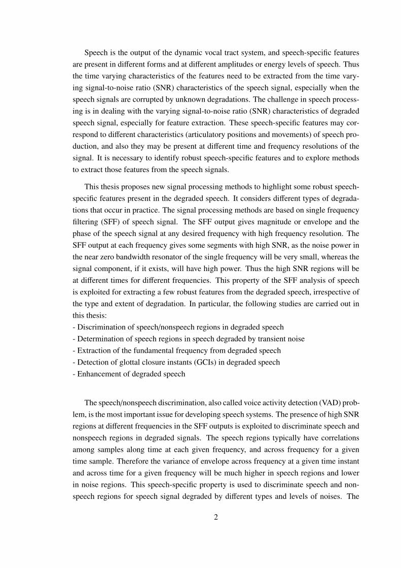
2.1 Block diagram of Adaptive Multi-rate (AMR) method. . . . . . . . . . 7

2.2 (a) Clean speech signal. (b) Speech signal corrupted by door knock noise.

(c) Spectrogram. . . . . . . . . . . . . . . . . . . . . . . . . . . . . . 9

4.1 (a) Clean speech signal. (b) Speech signal corrupted by pink noise at -10

dB SNR. (c) Envelopes as a function of time. (d) Corresponding weighted

envelopes. (e) Envelopes as a function of time for clean speech shown in

(a). . . . . . . . . . . . . . . . . . . . . . . . . . . . . . . . . . . . . . 25

4.2 (a) Clean speech signal. (b) Speech signal corrupted by pink noise at

-10 dB SNR. (c) µ[n]. (d) σ[n]. (e) σ[n] − µ[n]. (f) δ[n] along with sign.

(g) δ[n]. . . . . . . . . . . . . . . . . . . . . . . . . . . . . . . . . . . 27

4.3 (a) Clean speech signal. (b) Speech signal corrupted by pink noise at 5 dB

SNR. (c) µ[n]. (d) σ[n]. (e) σ[n]−µ[n]. (f) δ[n] along with sign. (g) δ[n]. 28

4.4 Histogram of ρ values for distant speech (C3). . . . . . . . . . . . . . . 30

4.5 Illustration of results of VAD for six different types of NOISEX data at

-10 dB SNR. Each noise type has three subfigures: Clean/Degraded signal

at -10 dB SNR, δ[n], and decision for the proposed method (thick line)

and for AMR2 method (thin line). Clean speech (a, b, c), White noise (d,

e, f), Babble noise (g, h, i), Volvo noise (j, k, l), Leopard noise (m, n, o),

Buccaneer1 noise (p , q, r), Buccaneer2 noise (s, t, u). The ground truth

is indicated on top of the clean speech signal in (a). . . . . . . . . . . . 36

ix

4.6 Illustration of results of VAD for six different types of NOISEX data at

5 dB SNR. Each noise type has three subfigures: Clean/Degraded signal

at 5 dB SNR, δ[n], and decision for the proposed method (thick line) and

for AMR2 method (thin line). Clean speech (a, b, c), White noise (d, e,

f), Babble noise (g, h, i), Volvo noise (j, k, l), Leopard noise (m, n, o),

Buccaneer1 noise (p, q, r), Buccaneer2 noise (s, t, u). The ground truth is

indicated on top of the clean speech signal in (a). . . . . . . . . . . . . 37

4.7 Illustration of results of VAD for seven different types of NOISEX data

at -10 dB SNR. Each noise type has three subfigures: Degraded signal

at -10 dB SNR, δ[n], and decision for the proposed method (thick line)

and for AMR2 method (thin line). Pink noise (a, b, c), Hfchannel noise

(d, e, f), m109 noise (g, h, i), f16 noise (j, k, l), Factory1 noise (m, n, o),

Factory2 noise (p, q, r), Machine gun noise (s, t, u). The ground truth is

indicated on top of the degraded speech signal in (a). . . . . . . . . . . 38

4.8 Illustration of results of VAD for seven different types of NOISEX data

at 5 dB SNR. Each noise type has three subfigures: Degraded signal at

5 dB SNR, δ[n], and decision for the proposed method (thick line) and

for AMR2 method (thin line). Pink noise (a, b, c), Hfchannel noise (d,

e, f), m109 noise (g, h, i), f16 noise (j, k, l), Factory1 noise (m, n, o),

Factory2 noise (p, q, r), Machine gun noise (s, t, u). The ground truth is

indicated on top of the degraded speech signal in (a). . . . . . . . . . . 39

4.9 (a) Distance speech (C0) with ground truth indicated on top. (b) δ[n]. (c)

Decision of the proposed method at η = 90% (solid line) and the AMR2

method (dotted line). . . . . . . . . . . . . . . . . . . . . . . . . . . . 40

4.10 (a) Distance speech (C3) with ground truth indicated on top. (b) δ[n]. (c)

Decision of the proposed method at η = 90% (solid line) and the AMR2

method (dotted line). . . . . . . . . . . . . . . . . . . . . . . . . . . . 41

5.1 (a) Clean speech signal. (b) Speech signal corrupted by door knock noise.

(c) Values of σ[n] (bold line) and θt[n] (dashed line). . . . . . . . . . . 50

5.2 (a) Clean speech signal. (b) Degraded speech signal corrupted by desk

thump noise at 0 dB SNR. (c) Variance (σ2[n]). (d) Differenced signal

(σ2d[n]). (e) Normalized peak amplitude. . . . . . . . . . . . . . . . . 54

5.3 (a) Clean speech signal. (b) Degraded speech signal corrupted by white

noise at at 0 dB SNR. (c) Variance (σ2[n]). (d) Differenced signal (σ2d[n]).

(e) Normalized peak amplitude. . . . . . . . . . . . . . . . . . . . . . 55

x

6.1 (a) Clean speech signal. (b) Envelope at 1 kHz derived as a function of

time for r = 0.995. (c) Envelope at 1 kHz derived as a function of time for

r = 0.95. (d) Spectral envelope at t = 0.5 sec for r = 0.995. (e) Spectral

envelope at t = 0.5 sec for r = 0.95. . . . . . . . . . . . . . . . . . . . 61

6.2 (a) Clean speech signal. (b) Speech signal degraded by white noise at

S NR = 0 dB. Normalized autocorrelation (AC) sequences derived from

(c) clean speech signal, (d) degraded speech signal, and by the proposed

method at (e) 360 Hz, (f) 460 Hz, (g) 560 Hz (FD), (h) 660 Hz, (i) 760 Hz.

The reference pitch period of the speech signal is 9.25 msec. The max-

imum peak in the autocorrelation sequence and its corresponding pitch

period location is indicated by a vertical arrow in each case. . . . . . . 65

6.3 (a) Clean speech signal. (b) Speech signal degraded by white noise at

SNR of 0 dB. (c) Dominant frequency (FD) contour. (d) Normalized peak

amplitude (θ). (e) Reference fo. (f) fo derived by the proposed method.

(g) fo derived by YIN method. . . . . . . . . . . . . . . . . . . . . . . 67

6.4 (a) Clean speech signal. (b) Speech signal degraded by volvo noise at

SNR of 0 dB. (c) Dominant frequency (FD) contour. (d) Normalized peak

amplitude (θ). (e) Reference fo. (f) fo derived by the proposed method.

(g) fo derived by YIN method. . . . . . . . . . . . . . . . . . . . . . . 68

6.5 (a) Clean speech signal. (b) Speech signal degraded by white noise at

0 dB SNR. (c) δ[n]. . . . . . . . . . . . . . . . . . . . . . . . . . . . . 76

6.6 Envelopes derived at a time instant for (a) r = 0.995, (b) r = 0.99, (c)

r = 0.95, and for (d) r = 0.9. . . . . . . . . . . . . . . . . . . . . . . . 80

7.1 (a) Clean speech signal. (b) Speech signal degraded by white noise at 0 dB

SNR. (c) Component envelopes. (d) Weighted component envelopes. . 83

7.2 (a) DEGG signal. (b) Clean speech signal. (c, d) Variance (σ2[n]) and

slope computed from envelopes derived from clean speech. (e) Speech

signal degraded by white noise at 0 dB SNR. (f, g) Variance and slope

computed from envelopes of degraded speech. (h, i) Variance and slope

computed from the compensated envelopes of degraded speech. . . . . 85

7.3 (a) DEGG signal. Values of slope derived from compensated envelopes

for the speech degraded at 10 dB SNR with (b) white noise, (c) babble

noise, (d) machine gun noise (e) f16 noise, (h) hfchannel noise. . . . . 86

xi

8.1 (a) Clean speech signal. (b) Speech degraded by white noise at 0 dB SNR.

(c) Gross weight function (g[n]). . . . . . . . . . . . . . . . . . . . . . 94

8.2 (a) Clean speech signal. (b) Degraded speech signal. (c) Fine weight

function ( f [n]). . . . . . . . . . . . . . . . . . . . . . . . . . . . . . . 95

8.3 (a) Speech degraded by white noise at 5 dB SNR. (b) Enhanced speech

signal. (c) Spectrogram of the degraded speech signal. (d) Spectrogram

of the enhanced speech signal. . . . . . . . . . . . . . . . . . . . . . . 95

8.4 (a) Speech degraded by babble noise at 5 dB SNR. (b) Enhanced speech

signal. (c) Spectrogram of the degraded speech signal. (d) Spectrogram

of the enhanced speech signal. . . . . . . . . . . . . . . . . . . . . . . 96

xii

Chapter 1

Introduction

Speech signals collected by a microphone in a practical environment are degraded in

several ways and by several types of noises. Apart from the degradations, speech may

be affected by the channel-induced distortions due to telephone or cellphone channels,

or by reverberation and other effects due to speech collected at a distance. Extraction

of the acoustic features of speech production from the speech signal is affected due to

these degradations in speech. Extracted features in turn affect the performance of speech

systems, such as automatic speech recognition and speaker recognition systems.

Speech recognition system consists mainly of two stages: Feature extraction from

speech signals and building a classification model based on the extracted features. Tradi-

tionally these systems deal with degradations in speech by mapping the extracted features

closer to the features extracted from the clean speech signal, and also by making changes

in the classification model according to the degradation. In many such cases, attempts are

made to derive the characteristics of degrading noise or channel. Thus there is an implicit

assumption that the characteristics of degradation are stationary over a long period of

time and also that there is mostly one type of degradation to deal with at a time. It is also

assumed that the characteristics of degradation are nearly same during training (i.e., de-

velopment of system) and during testing (i.e., actual usage). Moreover, it is expected that

all the features of the speech signal are affected in a similar fashion due to degradations.

In practice, the degradations in speech are not of the same type throughout, and there

could be multiple degradations at the same time. Hence it is not possible to improve the

performance of speech systems by feature transformation or mapping or by modifications

of the classification model. It is necessary to extract robust features from the degraded

speech by exploiting the characteristics of speech, as the nature and type of the degrada-

tion is not known in practice.

1

Speech is the output of the dynamic vocal tract system, and speech-specific features

are present in different forms and at different amplitudes or energy levels of speech. Thus

the time varying characteristics of the features need to be extracted from the time vary-

ing signal-to-noise ratio (SNR) characteristics of the speech signal, especially when the

speech signals are corrupted by unknown degradations. The challenge in speech process-

ing is in dealing with the varying signal-to-noise ratio (SNR) characteristics of degraded

speech signal, especially for feature extraction. These speech-specific features may cor-

respond to different characteristics (articulatory positions and movements) of speech pro-

duction, and also they may be present at different time and frequency resolutions of the

signal. It is necessary to identify robust speech-specific features and to explore methods

to extract those features from the speech signals.

This thesis proposes new signal processing methods to highlight some robust speech-

specific features present in the degraded speech. It considers different types of degrada-

tions that occur in practice. The signal processing methods are based on single frequency

filtering (SFF) of speech signal. The SFF output gives magnitude or envelope and the

phase of the speech signal at any desired frequency with high frequency resolution. The

SFF output at each frequency gives some segments with high SNR, as the noise power in

the near zero bandwidth resonator of the single frequency will be very small, whereas the

signal component, if it exists, will have high power. Thus the high SNR regions will be

at different times for different frequencies. This property of the SFF analysis of speech

is exploited for extracting a few robust features from the degraded speech, irrespective of

the type and extent of degradation. In particular, the following studies are carried out in

this thesis:

- Discrimination of speech/nonspeech regions in degraded speech

- Determination of speech regions in speech degraded by transient noise

- Extraction of the fundamental frequency from degraded speech

- Detection of glottal closure instants (GCIs) in degraded speech

- Enhancement of degraded speech

The speech/nonspeech discrimination, also called voice activity detection (VAD) prob-

lem, is the most important issue for developing speech systems. The presence of high SNR

regions at different frequencies in the SFF outputs is exploited to discriminate speech and

nonspeech regions in degraded signals. The speech regions typically have correlations

among samples along time at each given frequency, and across frequency for a given

time sample. Therefore the variance of envelope across frequency at a given time instant

and across time for a given frequency will be much higher in speech regions and lower

in noise regions. This speech-specific property is used to discriminate speech and non-

speech regions for speech signal degraded by different types and levels of noises. The

2

results are comparable or better than many of the state-of-the-art methods for VAD, for

several types of noises, as well as for far-field speech. The proposed method does not

make any assumptions of the type and level of the noise, nor it depends on any noise

dependent thresholds.

However, the performance of the proposed VAD method is not likely to be good for

several types of transient noises, which also have variance properties similar to speech.

Therefore the VAD for transient noise degradation in speech is addressed separately. Sev-

eral types of practical noises are considered. The VAD for speech degraded by both tran-

sient and other nonstationary types of noises is examined by exploiting some additional

speech characteristics such as voicing. The results obtained by the proposed SFF-based

methods are significantly better than some of the recent VAD methods proposed in the

literature for transient noises.

Another significant feature of speech is the fundamental frequency ( fo) of the glottal

excitation in voiced speech. fo estimation from speech is important not only for speech

and speaker recognition systems, but also for developing speech synthesis and speech en-

hancement systems. Several methods for fo estimation from degraded speech have been

developed over the past few decades. Most of the methods depend on autocorrelation of

the signal or modified signal to estimate the pitch period to =1fo

. A new approach for fo

estimation is proposed by exploiting the highest SNR segments in the SFF outputs. The

method involves selecting the higher SNR regions in the SFF outputs at several frequen-

cies. The SFF output that gives the highest SNR among all the frequency components for

a segment of speech is chosen for computing the pitch period (to) using autocorrelation

function. The resulting fo estimates are compared with the results from the state-of-the-art

methods. The proposed method gives comparable or significantly better results for most

cases of practical degradation.

Glottal closure instants (GCIs) are the instants of significant excitation of the vocal

tract system within a glottal cycle. Glottal vibration is the major source of excitation

resulting in voiced speech, which constitutes over 85% of speech. The impulse-like ex-

citation at GCIs is also responsible for producing high SNR speech regions within each

glottal cycle. Detection of GCIs in voiced speech is a major signal processing challenge

due to its instant property, but contributes to the one of the robust features of speech

signal. The GCIs help processing speech better. Large number of studies have reported

on the methods for detection of GCI, especially from degraded speech. Many of these

methods do not perform well due to their inability to estimate the vocal tract filter from

degraded speech. The vocal tract filter is used to estimate the excitation or the residual

signal, from which GCIs are estimated. In this thesis the high SNR output at each fre-

quency is exploited to detect GCIs without explicitly performing inverse filtering of the

3

speech signal.

Using the features used for speech/nonspeech detection, fo estimation, it is possible

to identify low and high SNR regions of speech as well as nonspeech regions in degraded

speech signal. Suitable gross weighting and fine weighting functions can be derived from

this information. The weighting functions are applied on the degraded signal to obtain

speech enhanced signal. The enhanced signal is subjected to listening tests to determine

the extent of speech enhancement from degraded signal for the comfort of listening. It

is shown that the proposed enhancement method significantly improves the comfort level

for listening in comparison with listening to degraded speech signal.

4

Chapter 2

Literature review of methods processing

degraded speech

This chapter gives a review of various methods for the tasks attempted in the thesis.

Speech/nonspeech detection or voice activity detection (VAD) is an important preprocess-

ing step for speech systems, and is required to be robust to degradations. Section 2.1 gives

a review of various methods attempted for voice activity detection (VAD). Section 2.2 ex-

plains the characteristics of transient noise and the limitations of the VAD methods to deal

with transient noises. Estimation of fundamental frequency ( fo) plays an important role

in many speech applications like speech coding, speaker recognition, etc. Performance

of the fo estimation methods deteriorated in the presence of degradations. Section 2.3 re-

views methods used for extraction of fundamental frequency ( fo) from degraded speech.

Section 2.4 gives a review of the methods used for detection of glottal closure instants

(GCIs). Precise estimation of the GCIs from degraded speech is difficult particularly due

to its instant properties. Section 2.5 reviews methods used for enhancement of degraded

speech. In the thesis, robust features are proposed for the speech tasks by using informa-

tion derived by the single frequency filtering (SFF) method.

2.1 Voice activity detection

The objective of voice activity detection (VAD) is to determine the regions of speech in

the acoustic signal, even in the presence of degradations. VAD is an essential first step for

development of speech systems such as speech and speaker recognition. Human listeners

are able to distinguish speech and nonspeech regions by interpreting the signal in terms of

speech characteristics, as well as the context. If a machine has to discriminate these two

5

regions, it has to depend on the characteristics of speech and degradation. It is difficult to

make a machine use the accumulated knowledge of a human listener for this purpose.

Robustness of a VAD method depends on

(a) the type of degradations,

(b) features extracted from the signal, and

(c) models used to discriminate speech and nonspeech regions.

The acoustic features are usually based on the signal energy in different frequency

bands, which includes the standard melfrequency cepstral coefficients (MFCC’s) used for

VAD [1]. Features based on speech characteristics such as voicing and dynamic spectral

characteristics are explored in [2], [3]. Energy-based features depend on the noise am-

plitude, and perform poorly when the amplitude of the noise matches the speech signal

energy. Some attempts have been made to explore features in the excitation component

of speech signal [4]. Features of the discrete wavelet transform and Teager energy op-

erator have been proposed for VAD with good results [5], [6]. New features like Multi-

Resolution cochleagram (MRCG) along with boosted Deep Neural Networks (bDNNs)

have been proposed for VAD, which are shown to outperform the state-of-the-art VADs

even at low SNRs, especially for babble and factory noises [7], [8].

Characteristics of speech and noise can be captured well if the samples are collected

over long (>1 sec) durations. Analysis of long term information was used for exploiting

the degree of non-stationarity of the signal for distinguishing speech from noise. The

characteristics of signal derived over long segments show a contrast between speech and

nonspeech at low SNRs. Spectral information is derived over short frames (eg 20 msec

duration), and then processed over long durations. However processing information over

long durations would decrease performance at high SNRs [9], [10], [11], [12].

The long-term divergence measure (LTDM) gives the spectral divergence between

speech and noise over longer duration [9]. The LTDM measure is calculated as the ratio

of the long-term spectral energies of speech and noise over different frequency bands.

The noise in different frequency bands was estimated from the initial nonspeech data.

The long-term spectral flatness measure (LSFM) is given by as the logarithm of the ra-

tio of arithmetic mean to geometric mean of the power specrtum over long frames [10].

Performance of this method degraded for nonstationary noises.

More recently, long-term spectral variability has been suggested for VAD [11]. The

variance across frequency of the entropy computed over a long frame (300 msec) of

speech at each frequency is termed as long-term signal variability (LTSV). The long-

term signal variability (LTSV) was extended to multi-band long-term signal variability to

accommodate multiple spectral resolutions [12]. The methods showed good performance

6

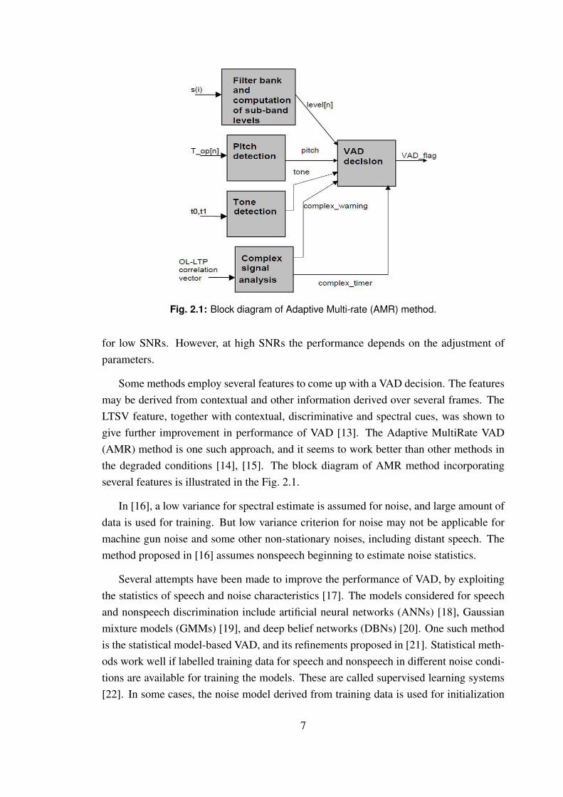
Fig. 2.1: Block diagram of Adaptive Multi-rate (AMR) method.

for low SNRs. However, at high SNRs the performance depends on the adjustment of

parameters.

Some methods employ several features to come up with a VAD decision. The features

may be derived from contextual and other information derived over several frames. The

LTSV feature, together with contextual, discriminative and spectral cues, was shown to

give further improvement in performance of VAD [13]. The Adaptive MultiRate VAD

(AMR) method is one such approach, and it seems to work better than other methods in

the degraded conditions [14], [15]. The block diagram of AMR method incorporating

several features is illustrated in the Fig. 2.1.

In [16], a low variance for spectral estimate is assumed for noise, and large amount of

data is used for training. But low variance criterion for noise may not be applicable for

machine gun noise and some other non-stationary noises, including distant speech. The

method proposed in [16] assumes nonspeech beginning to estimate noise statistics.

Several attempts have been made to improve the performance of VAD, by exploiting

the statistics of speech and noise characteristics [17]. The models considered for speech

and nonspeech discrimination include artificial neural networks (ANNs) [18], Gaussian

mixture models (GMMs) [19], and deep belief networks (DBNs) [20]. One such method

is the statistical model-based VAD, and its refinements proposed in [21]. Statistical meth-

ods work well if labelled training data for speech and nonspeech in different noise condi-

tions are available for training the models. These are called supervised learning systems

[22]. In some cases, the noise model derived from training data is used for initialization

7

process. These methods are called semi-supervised learning [17]. Methods based on uni-

versal models of speech, without assuming any specific type of noise, are also proposed

[23]. In [23], non-negative matrix factorization (NNMF) approach is used to develop uni-

versal speech model. In practice, it is preferable to develop a VAD algorithm that can

operate without any training data, i.e., unsupervised learning.

Most of the VAD methods are tested on data with simulated degradation, either by

adding noise or by passing the clean signal through a degrading channel. This is nec-

essary to evaluate new methods in comparison with known/existing methods. Very few

attempts have been made to assess the performance of a VAD algorithm with data col-

lected in practical environments. The degradations in such environments may not fit into

any standard model. Moreover, it is difficult to obtain ground truth in practice to evaluate

the VAD methods.

Most VAD methods usually estimate the characteristics of noise from the initial non-

speech data using nonspeech beginning criterion. Nonspeech beginning implies that the

initial data of the given degraded utterance is surely nonspeech/noise. The methods con-

sider data with nonspeech beginning for long durations (> 2 sec). The nonspeech begin-

ning criterion plays a significant role, as the statistical models are initiated and updated

with prior knowledge of the data being noise. In reality, the utterance/data may not have

nonspeech at the beginning or for long durations.

VAD methods usually depend on modelling the characteristics of noise, nonspeech

beginning criterion, and the availability of labelled training data. The types of degradation

present in the acoustic signal vary, and statistical models can not be modelled for every

case. The availability of training data in each case is not possible. Unsupervised methods

need to be developed without having any dependencies to work in different degradations.

A method for VAD is proposed in Chapter 4 extracting robust speech characteristics from

the degraded speech without relying on the estimation of the degradation characteristics.

2.2 Transient noise detection

Transient noises are usually characterized by impulsive nature, i.e., a sudden burst of

sound followed by decaying short-duration oscillations (eg gunshots, door knocks). Tran-

sient noises occupy several frequency bands. So VAD methods which bank on frequency

band selection to eliminate noisy frequency bands would not work. Normally, the it is

assumed that speech is more time-varying compared to nonspeech. This feature is con-

tradictory in the case of transient noise. In Fig. 2.2, the characteristics of transient noises

is illustrated through speech corrupted with door knock transient noise. The transient

8

noise is normalized to the maximum of speech amplitude, and added to the speech signal

(Fig. 2.2(b)). The corresponding clean speech is shown in Fig. 2.2(a). Fig. 2.2(c) shows

the spectrogram of door knock noise corrupted speech computed using a framesize of 30

msec with a frame shift of 1 msec. Notice that the chunks of door knock noise exhibit

a high temporal variance (Fig. 2.2(b)), and also that they also occupy a wide range of

frequencies (Fig. 2.2(c)).

Fig. 2.2: (a) Clean speech signal. (b) Speech signal corrupted by door knock noise. (c) Spectrogram.

VAD in the case of transient noises pose a severe challenge for online speech systems.

Several attempts have been made to identify and mask them for speech systems [24],

[25], [26]. In the case of recording of speech in a conference room, the presence of

transient noise would make the system interpret transient noise as speech of the dominant

speaker, and would record the transient noise as speech [27]. Recent methods tried to

compensate for the effects of the noise in speech by estimating long term characteristics

of noise [11], [12]. But it is difficult to identify transient noise regions. The features

which rely on long term statistics do not perform well in these noises because they would

further spread the noise characteristics into the neighbourhood regions and make them get

accepted as speech. The method in [13] using the long term spectral variability (LTSV)

measure did not give good results for machine gun noise (transient noise of bullet firing

sound). The multiband LTSV measure also fails in the case of transient noises [12]. From

these studies, it can be inferred that long term processing would not help in the case of

transient noise. Features derived from eigenvectors of normalized Laplacian and Gaussian

9

models are utilized to cluster speech and nonspeech discriminatively for detection of of

transient noise [28]. This is a supervised method, and involves training of models. Prior

data is needed to train the models. Some methods attempted transient noise detection

as identification of specific events like gun shots [25] and explosions [29]. Notice that

the methods were attempted for each type of transient noise, and statistical models were

separately trained for every type of transient noise.

Features extracted from the block-based methods, like discrete Fourier transform (DFT),

represent the averaged characteristics of the speech sounds present in that block (frame),

and do not correspond to the instantaneous behaviour of speech or noise. The method

proposed in Chapter 5 uses instantaneous features computed using the single frequency

filtering (SFF) method. The information captured at each sampling instant is able to dis-

criminate the impulsive transient noise from speech.

2.3 Extraction of fundamental frequency

Voiced speech is produced due to excitation caused by the vibration of vocal folds. The

pitch period (to) is the time interval of each cycle of the vocal fold vibration. The funda-

mental frequency ( fo) or the rate of vibration of the vocal folds is the inverse of the pitch

period (to). Estimation of fo is needed in applications such as speech synthesis [30], voice

conversion [31], gender recognition [32], speech coding [33], speaker recognition [34]

and speech recognition [35], voice controlled systems [36].

Time and frequency analysis methods have been proposed for estimation of the funda-

mental frequency (eg autocorrelation (AC) [37], crosscorrelation (CC) [38], robust algo-

rithm for pitch tracking (RAPT) [39], YIN [40], harmonic product spectrum (HPS) [41],

subharmonic-to-harmonic ratio (SHR) [42], sawtooth waveform inspired pitch estimator

(SWIPE) [43]). RAPT estimates the fo value as the local maxima of the energy normal-

ized crosscorrelation function [39]. The pitch extraction method used in the Kaldi ASR

toolkit uses a modified version of RAPT method. The Kaldi method does not make a hard

decision about voiced/unvoiced regions, and assigns an fo value even for the unvoiced

regions assuming continuous pitch trajectory [44]. YIN uses the difference function on

the amplitude values, followed by post processing technique to estimate the fo value [40].

The quasi-periodic nature of the speech signal in the time domain introduces peaks at the

fundamental frequency ( fo) and its harmonics in the frequency domain. Some methods

extract fo information from harmonics when the speech signal is degraded. The method

in [43] uses a weight function derived from the best peak-to-valley distance across its har-

monics to enhance the degraded harmonic structure to detect fo. The reliable fo harmonics

10

can be chosen based on the energy around each harmonic frequency [45].

Time-frequency based correlogram approaches have been proposed for fo estimation

in [46], [47]. Different comb filters were used in the low, mid and high frequency bands

to capture different sets of fo harmonics. The autocorrelation sequences derived from the

frequencies with higher harmonic signal energy were combined to get a summary cor-

relogram [46]. The peak in the summary correlogram indicated fo. Selection of reliable

frequencies in the correlogram was observed to improve the fo estimation [47], [48]. A

predetermined threshold was applied on the maximum amplitudes of the correlation se-

quences to select the reliable frequencies [48]. In some cases the cross-channel correlation

at selected frequencies was used to determine fo [49].

Zero-frequency filtering (ZFF) of speech signals was proposed for pitch period esti-

mation in [50]. The effects of vocal tract resonances and noise are suppressed, as they are

significant mainly in the frequencies much above 0 Hz. The zero-frequency filter consists

of an ideal resonator with four real poles on the unit circle in the z-plane, followed by a

trend removal operation. The positive zero crossings in the resulting ZFF output repre-

sent the instants of glottal closure, and the inverse of the time interval between successive

zero crossings in the ZFF signal represents the instantaneous fundamental frequency. The

method in [51] uses the refiltered ZFF signal for fo extraction in distant speech.

Statistical methods have also been proposed for fo estimation. Reliable subbands

were estimated from the training data in [52]. The influence of noise on the voiced

speech in different bands was learned and modelled from the training data in a proba-

bilistic framework [53]. The best pitch state sequence was derived using hidden Markov

models (HMMs) in [49]. The harmonics in the degraded speech were enhanced in the fre-

quency compressed and summation spectra derived over long term [54]. Neural networks

were then used to model the harmonic-based features across different noises [54]. The de-

rived filter output was given as input to deep neural networks (DNNs) and recursive neural

networks (RNNs) to predict the most probable fo value [55]. A multi-layered neural net-

work was trained on waveform vectors and pitch value to estimate harmonic structure

[56]. Such statistical methods are feasible only if the training data with annotations is

available.

The derived fo contour may be further processed to obtain best fit curves. Dynamic

programming based approaches were used to obtain the best fit curve from the derived

fo contour [46], [53],[57]. The rate of change of fo was limited for consecutive voiced

frames in [39]. Unvoiced regions were detected by voice activity detection (VAD) algo-

rithms, and were deemphasized in the estimation of fo [36], [58]. HMMs were used to

train acoustic models for voiced-unvoiced classification used as front-end for fo tracking

algorithm [36]. Such approaches are affected by the performance of the VAD system in

11

degraded conditions.

Selection of reliable frequencies in the correlogram was observed to improve the fo es-

timation [47], [48]. A predetermined threshold was applied on the maximum amplitudes

of the correlation sequences to select the reliable frequencies [48]. Statistical methods

have also been proposed for fo estimation. Reliable subbands were estimated from the

training data in [52]. The influence of noise on the voiced speech in different bands was

learned and modelled from the training data in a probabilistic framework [53]. The de-

rived fo contour may be further processed to obtain the best fit curves based on dynamic

programming approaches, and voiced-unvoiced decisions. TEMPO and PRAAT methods

determine voiced/unvoiced decisions based on the values of energy-based or harmonic-

based features using thresholds. However, the performance for different noises vary with

thresholds. The SNR-based weightage was used to select relevant fo candidates in [47],

analogous to other methods using voicing information to select reliable fo candidates.

However, it has been observed that detection of voiced-unvoiced decisions is not robust

across degradations, thus impacting the performance of fo methods. Ideally fo method

needs the correct estimation of voiced regions along with the accurate estimation of fo

values.

Performance of voice controlled systems are usually aided by an fo estimation algo-

rithm to make a precision estimation of the speaker’s voice. The rejection of improper

command plays an important role in such systems. For example, in the case of irreliable

speaker’s voice command it is acceptable to ask for a speaker’s voice once again rather

than proceeding inaccurately with a wrong interpretation. The reliability of the voiced

command is detected by using a voiced/unvoiced detection followed by fo estimation

[36], [46].

The method proposed in [57] for distant speech used artificial neural networks (ANNs)

on the denoised speech for voiced-unvoiced decision, followed by the Viterbi-based post-

processing on the derived fo contour. In [51], the ZFF signal was refiltered at the average

pitch frequency derived over longer segments. The method based on ZFF signal in [50]

uses NOISEX data, while the method in [51] uses the refiltered ZFF signal for fo ex-

traction from distant speech. The ZFF-based approaches do not work well for high pass

filtered speech like cellphone speech, as the method depends on the low (zero) frequency

component in the signal [50], [51]. It has been observed that fo methods like YIN, RAPT,

SHS, SHR, which worked for simulated degradations, did not perform well for distant

speech [51]. In general, we will not have prior information about the type of degradation

or environment.

Most of the current fo methods do not perform well across degradations, and they

performed poorly in the case of time varying degradations, particularly at low SNRs.

12

Methods have been proposed in Chapter 6 which exploits the high SNR segments of

speech at different frequencies for robust fo estimation.

2.4 Detection of glottal closure instants

Glottal closure instant (GCI) is the instant of significant excitation of the vocal tract, and

it occurs due to rapid closure of the vocal folds in each glottal cycle. Knowledge of the

GCI is useful for prosody manipulation in the voice conversion [59] and also in the text

to speech generation [60]. The signal around the GCI corresponds to high signal-to-noise

(SNR) region within a glottal cycle, and hence the features extracted around the GCIs

are more robust [61]. Several attempts have been made for detecting GCIs from speech

signals. Among them the peaks in the error signal of linear prediction (LP) analysis have

been exploited in many studies [59], [62]. Methods have been developed using group

delay functions and inverse filtering techniques for the detection of the GCIs [59], [63],

[64]. The Yet Another GCI/GOI Algorithm (YAGA) estimated the GCIs from the phase

slope function, followed by dynamic programming [64]. The Lines of Maximum Am-

plitude (LoMA) method uses the local maximum derived from the wavelet transform of

the multiscale product, followed by dynamic programming [65]. The subset of samples

with lowest singularity exponent values are used to detect the GCIs in the most singu-

lar manifold (MSM) method. It relies on the precise estimation of multiscale parameter

(singularity exponent) at each instant in the signal domain [66]. The Frobenius norm

offers a short-term energy estimate of the speech signal [67]. The Frobenius norm com-

puted using a sliding window gives an estimate of energy value at every speech sample.

The locations of peaks in the energy signal indicate glottal closure instants. A selection

function was defined based on speech signal and its Hilbert transform to give contrastive

information, which was used to separate the real epochs from the suboptimal epochs. The

zero frequency filtering (ZFF) is another approach proposed for GCI detection [68]. The

mean-based signal was computed over finite window to emphasize the discontinuities of

the speech signal to give intervals of GCI estimation in [69]. Most of these methods have

also been studied for varying levels and types of degradations in the speech signals. The

occurrence of glottal closure instants is abrupt with impulse-like characteristics, which is

used for its detection in Chapter 7.

13

2.5 Enhancement of degraded speech

Intelligibility and quality of speech suffer due to degradations in the speech signal. The

listener’s ability to understand speech decreases in the presence of degradations. Methods

have been developed to enhance the degraded speech. At the cognitive level, the context

of conversation and other features like intonation and duration aid in the perception of

speech even in degraded conditions. At the acoustic level, the speech signal is enhanced

by compensating for the effect of noise using various temporal and spectral features.

The Gaussian modeling of speech and noise spectral features combined with the Min-

imum Mean Square Error (MMSE) estimator is used in speech enhancement systems

[70]. The noise in various spectral bands is separated from speech using Independent

Component Analysis (ICA) [71]. Methods have been proposed to improve the quality of

speech signal in noisy environment, when the background noise exceeds the noise mask-

ing threshold [72]. The method proposed in Chapter 8 determines the gain functions at

the gross and fine levels to enhance the degraded speech.

2.6 Summary

In this chapter, several methods are discussed for VAD, estimation of fundamental fre-

quency ( fo), detection of glottal closure instants, and for enhancement of degraded speech.

Notice that most methods relied on the estimation of noise characteristics from the train-

ing data to perform in degraded conditions. Statistical models were used for VAD and

for enhancement to estimate the noise characteristics to suppress them. Most VAD meth-

ods relied on the nonspeech beginning assumption or the availability of labelled training

data to detect nonspeech. State-of-the-art fo methods may not perform well across degra-

dations. There are numerous degradations present across different environments whose

nature is not known aprior. Hence it is necessary to exploit speech-specific features from

the degraded speech. In the thesis, the high SNR segments of speech present at different

frequencies are exploited for this purpose.

14

Chapter 3

Single frequency filtering method

Speech signal has high signal-to-noise ratio (SNR) regions present at different times for

different frequencies. The chapter highlights the importance of processing speech at sin-

gle frequencies in order to capture the high SNR regions of the speech signal present at

different frequencies. The varying SNR characteristics of speech signal at different fre-

quencies are to be exploited to derive robust features from the degraded speech. In this

chapter, the single frequency filtering (SFF) method is proposed to derive the temporal

envelopes of the speech signal at the desired frequency with high resolution. The SFF

method uses a near-zero bandwidth resonator, and extracts information from the speech

signal (if present) at a particular frequency with high power. The amplitude envelopes

derived using the SFF method are further processed to derive speech-specific features for

the different studies attempted in the thesis.

3.1 Basis for processing speech at single frequencies

Speech signal has dependencies both along time and frequency. This results in signal to

noise power ratio to be a function of time as well as a function of frequency. For an ideal

noise (white noise) of a given total power, the power gets divided equally over frequency,

whereas for a signal, the power is distributed nonuniformly across frequency. ThusS 2( f )

N2( f )

is higher in some frequencies and lower in some other frequency regions, where S ( f ) and

N( f ) are signal and noise amplitudes as a function of frequency. This gives a much higher

value for the average ofS 2( f )

N2( f )over a frequency range, compared to the ratio of total signal

power to total noise power over the entire frequency range.

Let

15

α =

∫ fL

f0

S 2( f )

N2( f )d f , (3.1)

β =

L−1∑

i=0

∫ fi+1

fiS 2( f ) d f

∫ fi+1

fiN2( f ) d f

, (3.2)

and

γ =

∫ fL

f0S 2( f ) d f

∫ fL

f0N2( f ) d f

, (3.3)

where ( fi − fi+1) is the (i + 1)th interval of the L nonoverlapping frequency bands, and

i = 0, 1, ..., L − 1. The following inequality holds good.

α ≥ β ≥ γ. (3.4)

The S ( f ) and N( f ) are computed for a degraded speech utterance and for noise using

512-point DFT of Hann windowed segments of size 20 msec for every sample shift using

L = 16. In Table 3.1, the mean values α, β, γ of α, β and γ, respectively, computed over

the entire utterance are given. It is clear that α ≥ β ≥ γ for different types of noises. In

the case of uniform noise, (eg white), the values of α, β, γ are lower than the values for

the nonstationary noises (eg volvo and machine gun). In the case of some nonstationary

noises, the floor value is low at some frequencies which makes the denominator N( f )

small. With small values of the denominator, the ratios of α, β, γ are relatively higher, as

observed in Table 3.1 from the values ofα,β,γ for volvo and machine gun noises.

It is interesting to note that for nonuniformly distributed noises, such as machine gun,

f16 and volvo, α and β values are much higher than for the more uniformly distributed

noises, such as white, pink and buccaneer2, whereas the corresponding γ values are low

in all cases. This is due to regions having highS ( f )

N( f )in the time and frequency domains for

nonuniformly distributed noises. The signal and noise power as a function of frequency

can be computed using either discrete Fourier transform (DFT).

Table 3.2 shows that the inequality (3.4) holds good for SFF method (to be described

in section 3.2) also. It is inferred from Tables 3.1 and 3.2 that processing speech at single

frequencies preserves signal-to-noise ratio (SNR) better as indicated by the higher values

of α across all noises. The SFF method avoid effects due to block processing which is

crucial in estimation of more precise tasks like estimation of glottal closure events.

16

Table 3.1: Values ofα, β, γ computed using DFT method for speech signal degraded by differ-

ent noises at SNR of -10 dB for an entire utterance.

NOISE α β γ

white 2.289 1.1224 1.103

babble 237.4061 8.518 1.1481

volvo 3698.2985 233.7515 1.4089

leopard 1599.8217 35.0032 1.143

buccaneer1 277.1179 1.1356 1.1166

buccaneer2 5.4785 1.1299 1.0975

pink 2.2999 1.1034 1.1105

hfchannel 132.6712 1.8899 1.1094

m109 79.2124 2.4393 1.1294

f16 34927.2057 1.3335 1.1098

factory1 406.8931 1.2621 1.1199

factory2 66.5143 3.626 1.1703

machine gun 186034.6397 12056.4657 71.9059

Table 3.2: Values ofα, β, γ computed using SFF method for speech signal degraded by differ-

ent noises at SNR of -10 dB for an entire utterance..

NOISE α β γ

white 3.9853 1.1317 1.1034

babble 804.0397 3.992 1.1596

volvo 299.3464 44.2498 1.4496

leopard 117.9238 10.9565 1.156

buccaneer1 72.916 1.1395 1.1184

buccaneer2 3.1214 1.134 1.0978

pink 4.9493 1.1131 1.1112

hfchannel 17.8483 1.6226 1.1113

m109 59.2573 2.0275 1.1414

f16 18.2013 1.2939 1.1126

factory1 4.9478 1.2516 1.1235

factory2 21.4015 2.3495 1.1777

machine gun 10642.4183 753.7107 69.1977

17

3.2 Single frequency filtering (SFF) method

Single frequency filtering (SFF) method gives amplitude envelopes (ek[n]) at each sample

n at the selected frequency fk. with a pole close to the unit circle, and extracts information

at the highest carrier frequency (i.e., half the sampling frequency). Since the same filter

at a fixed frequency is used to derive the amplitude envelopes at different frequencies,

it avoids the different gain effects, if separate filters were chosen for each frequency to

derive amplitude information. The shape of the filter and its gain vary if different filters

are designed to extract information at different frequencies as in the case of filter bank

approaches (eg gammatone filter bank method [73]). The SFF method is explained below.

The discrete-time speech signal x[n] at the sampling frequency fs is multiplied by a

complex sinusoid of a given normalized frequency ωk to give xk[n]. The time domain

operation is given by

xk[n] = x[n]e jωkn, (3.5)

where

ωk =2π fk

fs

. (3.6)

Since x[n] is multiplied with e jωkn to give xk[n], the resulting spectrum of xk[n] is a shifted

spectrum of x[n]. That is,

Xk(ω) = X(ω − ωk), (3.7)

where Xk(ω) and X(ω) are spectra of xk[n] and x[n], respectively.

The signal xk[n] is passed through a single-pole filter, whose transfer function is given by

H(z) =1

1 + rz−1. (3.8)

The single-pole filter has a pole on the real axis at a distance of −r from the origin. The

root is located at z = −r in the z-plane, which corresponds to half the sampling frequency,

i.e., fs/2. The value of r is chosen as 0.99 for most cases in the study. The output yk[n] of

the filter is given by [74]

yk[n] = −ryk[n − 1] + xk[n]. (3.9)

The envelope of the signal ek[n] is given by

ek[n] =√

ykr2[n] + yki

2[n], (3.10)

where ykr[n] and yki[n] are the real and imaginary components of yk[n]. Since filtering of

xk[n] is done at fs/2, the envelope ek[n] corresponds to the envelope of the signal xk[n] at

18

the desired frequency given by

fk =fs

2− fk. (3.11)

A near zero bandwidth is achieved by placing the pole of the single-pole filter close the

unit circle in the z-plane (at z = −0.99). The resulting envelopes of the speech signal

would have high amplitudes if the speech signal has components corresponding to the

frequency fk.

19

Chapter 4

Speech/nonspeech discrimination in

degraded speech

Features derived from spectral and temporal characteristics of degraded speech, followed

by statistical model representation are used to discriminate speech and nonspeech regions.

Training of statistical models using Gaussian mixture models (GMMs), hidden Markov

models (HMMs), deep neural networks (DNNs), etc, has gained prominence in the re-

cent years. Models are trained for each type of noise and at each SNR. Availability of

labelled training data in each environment is not possible. Some methods try to estimate

the characteristics of nonspeech from the initial seconds of the degraded speech utterance,

assuming it to be only nonspeech. The nonspeech beginning criteria is not always true.

In reality, the characteristics of the degradations are not known aprior and hence can not

be estimated.

There have been several attempts for voice activity detection (VAD), reporting the per-

formance mainly on a limited set of simulated degradations. Simulated degradations are

degradations captured in a particular environment, and then added to the speech signal to

simulate the effect of degradation (eg NOISEX degradations [75]). Performance of VAD

methods relied on modelling specific characteristics of the degradation. A set of simulated

degradations can not capture the effect of numerous degradations present in practical en-

vironments. Rather than relying on the estimation of the characteristics of degradation, it

is necessary to extract robust speech-specific features from degraded speech to use it for

VAD. In this chapter, a VAD method is proposed exploiting signal-to-noise ratio (SNR) of

speech at each frequency. Since the method exploits the properties of the speech signal,

it is not necessary to have training data of speech and nonspeech signals to build models.

Also the proposed method does not rely on appended silence/noise regions to estimate

noise characteristics. The method is tested using simulated degradations on speech sig-

20

nals, and also using speech signals collected in practical environments. The proposed

method was able extract speech characteristics better due to the robust features used, and

performed well compared to the state-of-the-art methods.

The temporal envelopes of the speech signal at each frequency is compensated for

the effect of noise by determining a weight factor based on the noise floor. The noise

floor is created due to the uncorrelatedness of the noise samples. Speech signal has high

correlations among its samples due to its production mechanism, and exhibits high signal-

to-noise ratio at some frequencies. The proposed method exploits the high SNR charac-

teristics of speech signal at several single frequencies to derive a robust speech feature

denoted as δ[n]. The mean and variance of the weighted envelopes across frequency at

each sampling instant are used to derive a parameter contour (δ[n]) as a function of time,

and it is used to discriminate between speech and nonspeech regions. An adaptive thresh-

old is derived from the parameter contour for each utterance, followed by a decision logic

based on the features of speech and noise in the given utterance.

Many studies in literature compare VAD methods with the Adaptive Multi-Rate (AMR)

method [14], [15]. The comparison is done mainly at the score level. To have a fair com-

parison with the AMR method, the VAD methods should consider the following other

factors of the AMR method into account:

• Adaptability: AMR method is adaptable to various types of noise, SNRs and envi-

ronments.

• No prior information: It does not require training data or any other prior information

about the type of noise.

• Automatic threshold: The threshold estimation does not require nonspeech begin-

ning, and also does not use data for training of statistical models.

The AMR method with all its factors is used as a bench mark for comparison by the VAD

methods to assess the performance (eg [11]).

In section 4.1, speech data collected in different types of degradation is described.

Section 4.2 gives the development of the proposed VAD method. Section 4.3 explains

evaluation parameters of the VAD method. Section 4.4 gives the performance of the

SFF-based method of VAD in comparison with the AMR2 method for different types of

degradations. In section 4.5, different values are explored for the parameters used by the

proposed method to achieve the best performance in each case. Section 4.6 discusses the

relative performance of SFF, DFT and gammatone filtering methods for deriving informa-

tion in different frequency bands. In section 4.7, the proposed VAD method is compared

with LTSV method in terms of performance and other adaptability criteria. Section 4.8

21

gives a summary of this study.

4.1 Different types of degradation

In this section, different speech and noise databases and their characteristics are discussed

to indicate the variety of degradations considered for evaluation of the proposed VAD

method. Note that, although some of the data was collected at 16 kHz sampling rate and

other data at 8 kHz sampling rate, the frequencies in the range 300 - 4000 Hz only are

considered.

4.1.1 Adding degradation at different SNRs to clean speech signal.

The TIMIT test corpus is used for evaluation [76]. The sampling rate is 16 kHz. A VAD

method should ideally accept speech and also reject nonspeech. In a situation where there

is more duration of speech than nonspeech, then if the method has a higher speech accep-

tance, then the method shows better performance even if the performance of nonspeech

rejection is poor. A similar situation of better performance would arise for longer dura-

tion of nonspeech, with higher nonspeech detection rate and lower speech detection rate

of the method. To overcome this problem, each TIMIT utterance is appended with 2 sec

of silence at the beginning and end of the utterance as in [11]. Various samples of the

thirteen types of noises from NOISEX-92 database [75] are added to the clean TIMIT

speech signal at SNRs of -10 dB and 5 dB, to create degraded speech signals. The TIMIT

data provides boundaries of the phone labels, which are generated automatically and are

then hand corrected by experienced acoustic phoneticians. Hence these boundaries are

used as ground truth for comparing the results of the proposed VAD method on the noisy

speech data. The silence and pause labels are considered as nonspeech.

Most VAD methods use post processing techniques like hangover scheme. The hang-

over scheme is used to reduce the risk of lower energy regions of speech at the ends of

speech regions being falsely rejected [16]. This is based on the assumption that speech

frames are highly correlated in time [16], [17]. In hangover schemes decisions at the

frame level are smoothed by considering sequence of frames to arrive at a final decision.

Hangover schemes are applied to the VAD method after the initial VAD decision. In some

regions, the features of speech might not be evident even in clean speech, although those

regions are labelled as speech in the database. The ground truth given in TIMIT database

may not be a perfect reference for comparing results of any VAD method. This may be

due to mismatch between the perceptual evidence and speech data in manual labelling.

22

This is because of some cases in the database where nonspeech is labelled as speech

and vice-versa, as the speaker did not articulate some of the speech properly. Hence the

accuracy will not be 100% even in the case of clean speech.

4.1.2 Telephone channel database.

NTIMIT (Network TIMIT) database [77] was collected by transmitting TIMIT data over

telephone network. Speech utterances are transmitted from a laboratory to a central office

and then back from the central office to the laboratory, thus creating a loopback telephone

path from laboratory to a large number of central offices. These central offices were ge-

ographically distributed to simulate different telephone network conditions. Half of the

TIMIT database was sent over local telephone paths, while the other half was transmitted

over long distance paths. All recordings were done in an acoustically isolated room. The

NTIMIT test corpus is used for VAD evaluation. The sampling rate is 16 kHz. In the

NTIMIT case, 2 sec silence segments are not appended to the data, as this kind of degra-

dation can not be simulated in the appended regions. The ground truth for the NTIMIT is

same as for the TIMIT data.

4.1.3 Cellphone channel database.

The CTIMIT read speech corpus [78] was designed to provide a large phonetically-

labelled database for use in the design and evaluation of speech processing systems op-

erating in diverse, often hostile, cellular telephone environments. CTIMIT was generated

by transmitting and redigitizing 3367 of the 6300 original TIMIT utterances over cellu-

lar telephone channels from a specially equipped van, in a variety of driving conditions,

traffic conditions and cell sites in southern New Hampshire and Massachussetts. The

recorded data was played in the van over a loudspeaker and cellular handset combination.

Each received call was digitized at 8 kHz, segmented and time-aligned with the original

TIMIT utterances. The ground truth of TIMIT labels can be used here also. CTIMIT test

corpus is used for VAD evaluation [78]. Note that here also the 2 sec silence segments are

not appended to the data, as in the case of NTIMIT database.

4.1.4 Distant speech.

Differences between the characteristics of speech signal collected by a distant microphone

(DM) and that collected by a close-speaking microphone (CM) are as follows: (a) The

effects of radiation at far-field are different from those at the near-field. (b) The SNR is

23

lower in the DM speech signal due to additive background noise. (c) The reverberant

component in the DM speech signal is also significant, due to reflections, diffuse sound

and reduction in amplitude of the direct sound. (d) The DM speech signal may also be

affected due to interference from speech of other speakers present in the room. Hence, the

acoustic features derived from the DM speech signal are not same as those derived from

the corresponding CM speech signal.

Speech signals from SPEECON database are used for evaluation of the VAD method

for distant speech [79]. The signals were collected in three different cases, namely, car

interior, office and living rooms (denoted by public). The signals were collected simulta-

neously using a close-speaking microphone (a microphone placed just below the chin of

the speaker), and microphones placed at a close distance, and at distances of 1-2 meters

and 2-3 meters from the speaker. These four cases are denoted by C0, C1, C2 and C3,

respectively. Each case has 1020 utterances. Speech signals collected in the office envi-

ronment are affected by noises generated by computer fans and air-conditioning. Speech

signals collected in living rooms are affected by babble noise and music (due to radio or

television sets). Reverberation is present mostly in the office and living room environ-

ments. The estimated reverberation time in these environments varied from 250 msec to

1.2 sec. The average SNR measured at the close speaking microphone (C0) was around

30 dB, while that measured at distances of 2 meters to 3 meters was in the range 0 to 5 dB.

The database consists of speech signals collected from 30 male and 30 female speakers.

For each speaker, 17 utterances were recorded, resulting in about one minute of speech

data per speaker. People were asked to record free spontaneous items, elicited sponta-

neous items, read speech and core words. A manual voiced-unvoiced-nonspeech labels

are marked for every 1 msec in the SPEECON database for the C0 case. Since speech at

all the distances are simultaneously collected, the same labels are used for the data at all

distances. The manual labels (voiced-unvoiced labels for speech and nonspeech label for

the rest) form the ground truth for the data at all distances. The sampling rate is 16 kHz.

Since the utterances of each speaker are from different environments, it is not possible to

build statistical models with this kind of data. No silence data is appended in this case

also.

4.2 Proposed VAD method

The proposed VAD method implements a noise-compensation technique developed for

reducing the effect of noise at each frequency. The mean and variance of the noise-

compensated weighted envelopes are exploited to derive a robust feature δ[n]. Decision

logic is applied to the δ[n] values by optimizing parameters based on a dynamic range

24

parameter ρ to arrive at the VAD decision.

Fig. 4.1: (a) Clean speech signal. (b) Speech signal corrupted by pink noise at -10 dB SNR.

(c) Envelopes as a function of time. (d) Corresponding weighted envelopes. (e) Envelopes as

a function of time for clean speech shown in (a).

4.2.1 Weighted envelopes of speech signal.

The envelopes are computed at every 20 Hz for the differenced speech signal x[n] in the

range 300 Hz to 4000 Hz as a function of time. The frequency range 300 - 4000 Hz is

chosen, as it covers the useful spectral band of speech. Thus we have envelopes for 185

frequencies as a function of time.

25

Since speech signal has large dynamic range in the frequency domain, the signal may

have high power at some frequencies at each instant. At those frequencies the SNR will

be higher, as the noise power is likely to be less due to more uniform distribution of the

power. Even for noises with nonuniform distribution of power, the lower correlations

of noise samples result in a lower dynamic range in the spread of noise power across

frequencies, compared to speech. Note that the spectral dynamic range gives an indication

of the correlation of the samples in the time domain.

The noise power creates a floor for the envelope at each frequency, and the floor

level depends on the power distribution of noise across frequency. The floor is more

uniform across time if the noise is nearly stationary. Even if the noise is nonstationary, it

is relatively stationary over larger intervals of time than in speech. In such cases, the floor

level can be computed over long time intervals at each frequency, if needed.

To compensate for the effect of noise, a weight value at each frequency is computed

using the floor value. For each utterance, the mean (µk) of the lower 20% of the values of

the envelope at each frequency fk is used to compute the normalized weight value wk at

that frequency. The choice of 20% of the values is not critical and can vary from 10 - 40

%. The normalized weight value at each frequency is given by

wk =

1µk∑N

l=11µl

, (4.1)

where N is the number of channels. The envelope ek[n] at each frequency fk is multi-

plied with the weight value wk to compensate for the noise level at that frequency. The

resulting envelope is termed as weighted envelope. Note that by this weighting, the enve-

lope at each frequency is divided by the estimate of the noise floor (µk). Fig. 4.1 shows

the envelopes and the corresponding weighted envelopes at different frequencies for a

speech signal degraded by pink noise at -10 dB SNR, along with the envelopes for clean

speech. It is observed that features of speech are reflected better in the weighted envelopes

(Fig. 4.1(d)), as the weighting reduces the effects of noise. The envelopes are scaled to the

same value for comparison. A small amount of white noise (at 100 dB SNR) is added to

all the signals (after appending with zeros in the case of TIMIT utterances) to ensure that

the floor value is not zero. Some methods use the appended silence regions to train for

nonspeech characteristics. In practice given a degraded utterance, silence regions can not

be appended as the degradation characteristics can not be synthesized (as in the case of

distant speech). So the proposed method does not consider values in the appended silence

regions for the computation of wk.

26

4.2.2 Computation of δ[n] values

-1

0

1 (a) Clean speech signal

-1

0

1 (b) Degraded signal

0

1

2 10 -4

(c) [n]

0

2

4 10 -4

(d) [n]

0

2

410 -4

(e) [n] - [n]

-0.5

0

0.5

1(f) [n] with sign

0 0.5 1 1.5 2 2.5 3 3.5Time(sec)

0.5

1(g) [n]

Fig. 4.2: (a) Clean speech signal. (b) Speech signal corrupted by pink noise at -10 dB SNR.

(c) µ[n]. (d) σ[n]. (e) σ[n] − µ[n]. (f) δ[n] along with sign. (g) δ[n].

At each time instant, the mean (µ[n]) of the square of the weighted envelopes com-

puted across frequency corresponds approximately to the energy of the signal at the instant

(Fig. 4.2(c)). The µ[n] is expected to be higher for speech than for noise in the regions

where speech signal is present, as the noise signals are deweighted. At each time instant,

the standard deviation (σ[n]) of the square of the weighted envelopes computed across

frequency will also be relatively higher for speech than for noise in the regions of speech

due to formant structure (Fig. 4.2(d)). Hence (σ[n]+µ[n]) is generally higher in the speech

regions, and lower in the nonspeech regions. Since the spread of noise (after compensa-

tion) is expected to be lower, it is observed that the values of (σ[n] − µ[n]) are usually

lower in the nonspeech regions compared to the values in the speech regions (Fig. 4.2(e)).

Multiplying (σ[n] + µ[n]) with (σ[n] − µ[n]) gives (σ2[n] − µ2[n]), which highlights the

contrast between speech and nonspeech regions. Figs. 4.2 and 4.3 illustrate the features

of µ[n], σ[n] and (σ[n] − µ[n]) for an utterance corrupted by pink noise at SNR = -10 dB

and SNR = 5 dB, respectively.

27

-1

0

1 (a) Clean speech signal

-1

0

1 (b) Degraded signal

0

1

2 10 -4

(c) [n]

0

2

4 10 -4

(d) [n]

-0.50

0.51 (f) [n] with sign

0 0.5 1 1.5 2 2.5 3 3.5Time(sec)

0.5

1(g) [n]

-2024

10 -4

(e) [n] - [n]

Fig. 4.3: (a) Clean speech signal. (b) Speech signal corrupted by pink noise at 5 dB SNR. (c)

µ[n]. (d) σ[n]. (e) σ[n] − µ[n]. (f) δ[n] along with sign. (g) δ[n].

Due to large dynamic range of the values of (σ2[n] − µ2[n]), it is difficult to observe

the speech regions with small values of (σ2[n]−µ2[n]). To highlight the contrast between

speech and nonspeech regions, the dynamic range is reduced by computing

δ[n] =M√|(σ2[n] − µ2[n])|, (4.2)

where M is chosen as 64.

The value of M is not critical. Any value of M in the range of 32 to 256 seems to pro-

vide good contrast between speech and nonspeech regions in the plot of δ[n]. In comput-

ing δ[n], only the magnitude of (σ2[n]−µ2[n]) is considered. If the sign of (σ2[n]−µ2[n])

is assigned to δ[n], the values will be fluctuating around zero in the nonspeech regions

for most types of noise (see Fig. 4.2(f) for pink noise), but the short time (20 - 40 msec)

temporal average value will be small and fluctuating, making the noise floor uneven. This

makes it difficult to set a threshold for deciding nonspeech regions. The values of δ[n]

will have a high temporal mean value in the nonspeech regions, with small temporal vari-

ance (Fig. 4.2(g)). This helps to set a suitable threshold to isolate nonspeech regions from

28

speech regions. The range of δ[n] with sign value (Fig. 4.2(f)) is different from δ[n] values

(Fig. 4.2(g)). The small temporal spread of δ[n] values in the nonspeech regions and its

mean value helps to fix a suitable threshold. The δ[n] values in the nonspeech regions is

dictated by the noise level. The δ[n] values in nonspeech regions are high for pink noise

degradation at -10 dB SNR (Fig. 4.2(g)) than at 5 dB SNR (Fig. 4.3(g)). Note that, by

considering the δ[n] values without sign, we are losing some advantage in the discrimi-

nation of nonspeech regions, which has both positive and negative values, compared to

speech regions which have mostly positive values. The δ[n] values with M = 64 are

used for further processing for decision making. Note the changes in the vertical scales in

Figs. 4.2(f) and 4.2(g), and also in Figs. 4.3(f) and 4.3(g), to understand the significance

of using the absolute value, i.e., δ[n] without sign.

4.2.3 Decision logic.

The decision logic is based on δ[n] for each utterance, by first deriving the threshold over

the assumed (20% of the low energy) regions of noise, and then applying the threshold on

temporally smoothed δ[n] values. The window size lw used for smoothing δ[n] is adapted

based on an estimate of the dynamic range (ρ) of the energy of the noisy signal in each

utterance, assuming that there is at least 20% silence region in the utterance. The binary

decision of speech and nonspeech at each time instant, denoted as 1 and 0, respectively, is

further smoothed (similar to hangover scheme) using an adaptive window, to arrive at the

final decision. The following 5 steps describe the implementation details of the decision

logic:

1. Computation of threshold (θ):

Compute the mean (µθ) and variance (σθ) of the lower 20% of the values of δ[n] over

an utterance. A threshold of θ = µθ + 3σθ is used in all cases. The θ value depends

on each utterance. Thus the threshold value, corresponding to the floor value of

δ[n], is adapted to each utterance, depending on the characteristics of speech and

noise in that utterance.

2. Determination of smoothing window lw:

The energy Em of the signal x[n] is computed over a frame of 300 msec for a frame

shift of 10 msec, where m is the frame index. The dynamic range (ρ) of the signal

is computed as

ρ = 10 log10

maxm (Em)

minm (Em). (4.3)

The window length parameter lw for smoothing is obtained from the dynamic range

(ρ) of the signal. Table 4.1 gives the ρ values for degraded speech at SNRs of -10 dB

29

and 5 dB for different noises. The ρ values are high at 5 dB SNR compared to the

values at -10 dB SNR for the same noise. The ρ values vary for different noises for

the same SNR, because the degradation characteristics of noises vary. For distance

speech, the histogram of ρ values for utterances in the C3 case is shown in Fig. 4.4.

Table 4.1: Values of ρ for speech signal degraded at SNRs of -10 dB and 5 dB for different

types of noises. The value for clean speech is 65.28.

NOISE -10 dB SNR 5 dB SNR

white 14.90 22.61

babble 19.64 36.36

volvo 41.62 56.79

leopard 27.77 43.22

buccaneer1 16.13 28.36

buccaneer2 15.67 22.75

pink 16.73 27.60

hfchannel 16.68 28.46

m109 22.44 35.87

f16 17.84 28.88

factory1 20.48 36.28

factory2 24.13 36.30

machine gun 40.52 64.84

10 20 30 40 50 60 70 800

0.2

0.4

0.6

0.8

1

ρ

No

rmalised

fre

qu

en

cy

Fig. 4.4: Histogram of ρ values for distant speech (C3).

The SNR for distant speech depends on the environmental conditions and on the

distance of the speaker from microphone. It is observed that the ρ values for the

distant speech are spread out, compared to the ρ values for different noises. This

is mainly due to the effects of reverberation. The distribution of ρ values depends

on the distance as well. The ρ value for each utterance is used to determine some

parameter values for further processing of δ[n] and for arriving at the decision logic.

In cases where the δ[n] represent the discriminating characteristics of speech and

nonspeech well, the corresponding ρ values are high, as observed for volvo, leopard

and machine gun noises. In such cases, small value of the smoothing window pa-

rameter lw is used. The following values of lw are chosen based on experimentation

30

with speech degraded by different types of noises at different SNR levels:

lw = 400 msec, for ρ < 30. (4.4)

lw = 300 msec, for 30 <= ρ <= 40. (4.5)

lw = 200 msec, for ρ > 40. (4.6)

3. Decision logic at each sampling instant:

The values of δ[n] are averaged over a window of size lw to obtain the averaged

value δ[n] at each sample index n. The decision d[n] is made as follows:

d[n] = 1, for δ[n] > θ. (4.7)

d[n] = 0, for δ[n] ≤ θ. (4.8)

4. Smoothing decision at the sample level:

The decision d[n] at each sample is processed over windows of size 300 msec, 400

msec and 600 msec, respectively, for the 3 ranges of ρ indicated in (4.4), (4.5) and

(4.6). Let η be the threshold on the proportion (in percentage value) of d[n] values

which are 1 in the window. If the percentage of d[n] values which are 1 in the

window is above the η value, then the final decision d f [n] is made 1 at the sampling

instant n, otherwise it is 0. The value assigned to η is 60%.

5. Decision at frame level:

The decision of the AMR methods is given for every 10 msec frame [15]. In order

to compare the proposed method with the AMR method, the decision d f [n] is con-

verted to a 10 msec frame based decision. For each 10 msec nonoverlapping frame,

if majority of d f [n] values are 1, then the frame is marked as speech, otherwise it is

marked as nonspeech. The ground truth of speech signals is also derived for each

10 msec frame.

4.3 Parameters for evaluation of the VAD methods

The proposed method is compared with the state-of-the-art AMR1 and AMR2 methods

[15]. AMR1 and AMR2 methods extract subband energies using filter banks. Several

acoustical features like pitch, tone, etc, are used to arrive at the decision. Post-processing

techniques like hangover are also used [14]. We use the recent version 3GPP TS 26.104

of the AMR methods [15].

We use 5 parameters to evaluate the proposed method against AMR methods for com-

parison [80].

31

• CORRECT: Correct decisions made by the VAD.

• FEC (front end clipping): Clipping due to speech being misclassified as noise in

passing from noise to speech activity.

• MSC (mid speech clipping): Clipping due to speech being misclassified as noise

during a speech region.

• OVER (carry over): Noise interpreted as speech in passing from speech activity to

noise.

• NDS (noise detected as speech): Noise interpreted as speech within silence/noise

region.

All the above parameters are divided by the total number of frames (both speech and

nonspeech frames), and then multiplied by 100 to get the percentage value (%). Combin-

ing FEC and MSC gives true rejection (TR). Combining OVER and NDS gives false ac-

ceptance (FA). The TR indicates the percentage of speech regions not detected as speech,

whereas the FA indicates the percentage of nonspeech regions accepted as speech. For

good performance, CORRECT should be high, and both TR and FA should be low.

4.4 Performance of the proposed VAD method

Tables 4.3 - 4.6 show the performance of the proposed method (PM) in comparison with

the AMR2 method for different type of degradations and at different SNR conditions.

The best performance in each case is indicated by boldface for CORRECT score. The

AMR2 method performs better than AMR1 method in all cases, which is evident from

the averaged scores across all noise types for the two different SNRs given in Table 4.2.

Hence we only consider AMR2 scores for comparison.

Table 4.2: Averaged scores across all noise types for two SNR levels for TIMIT database.

SNR (dB) METHOD CORRECT FEC MSC OVER NDS

-10 PM 79.11 0.06 15.21 0.03 5.49

AMR2 72.60 0.07 19.31 0.04 7.86

AMR1 51.70 0.02 2.50 0.10 45.56

5 PM 95.36 0.02 2.27 0.05 2.20

AMR2 88.85 0.04 2.31 0.09 8.58

AMR1 76.05 0.04 1.52 0.09 22.17

32

4.4.1 Performance on TIMIT database for different types of noises

at different SNRs.

Performance of the proposed method under different noise conditions of NOISEX database

is given in Table 4.3 for two different SNR values, i.e., at -10 dB and 5 dB. In the follow-

ing, the performance of the proposed method is discussed for different types of degrada-

tion.

The performance of the proposed method is higher than that of AMR2 method for all

types of noises. The performance is illustrated for different noises by an utterance in the

form of plots shown in Figs. 4.5 - 4.8 at SNRs of -10 dB and 5 dB. For each type of noise,

the degraded signal, the corresponding δ[n] values and the derived VAD decision (thick

line) are shown. In addition, the AMR2 decision is also shown by thin solid lines for

comparison. The ground truth is marked on the top subplot by a thin line. At low SNRs

most speech characteristics were immersed in the noise characteristics.

Many speech regions were missed by the AMR2 method for white noise case (Figs.

4.5(d), 4.6(d)), resulting in high TR. In the case of babble noise at 5 dB SNR at 5 dB SNR,

the amplitudes of speech regions is more than the amplitude of nonspeech regions, which

gives a high performance (91.72% compared to 74.12% CORRECT score for the AMR2

method (Fig. 4.8(r))). Performance of the proposed method is higher than the AMR2

method even at -10 dB SNR for these noises. Since most of the energy is concentrated in

the low frequency regions for volvo and leopard noises, it is relatively easier to reduce the

effect of this type of noise, and hence the proposed method performs better (Figs. 4.5(i,

o), 4.6(i, o)).

A significant lower TR is seen in the case of pink noise for the proposed method com-

pared to the AMR2 method. This is due to attenuation of noise regions by weighting. This

can also be seen in the 3D plots given in Fig. 4.1. Buccaneer noises are jet noises whose

error lies mostly in the TR. The proposed method is able to extract the speech characteris-

tics better, and hence performed higher compared to AMR methods (Figs. 4.5(r, u), 4.6(r,

u)). Speech characteristics lost due to f16 noise (noise recorded in cockpit) were also ex-

tracted better by the proposed method showing a lesser TR (Figs. 4.7(i), 4.8(i)). Factory

noises were recorded near plate-cutting and electrical welding equipment, and are non-

stationary noises. However the proposed technique is able to compensate for the noise

effect (Figs. 4.7(o, r), 4.8(o, r)). Due to its high temporal variance, most VAD algorithms

detect the machine gun chunks as speech. It is interesting to see in Figs. 4.7(u) and 4.8(u)

that the nonspeech regions affected by the machine gun noise are identified as nonspeech

by the proposed method, whereas the AMR2 method accepts them as speech. The LTSV

method proposed in [11] shows poor performance for this noise. The multi-band LTSV

33

method [12] also fails to discriminate the machine gun transient noise from speech.

34

Table 4.3: Evaluation results of the proposed VAD method (PM) for TIMIT database for differ-

ent types of noises at two SNR levels in comparison with AMR2 method

NOISE (SNR) METHOD CORRECT FEC MSC OVER NDS

white PM 77.60 0.08 21.99 0.01 0.23

(-10) AMR2 63.23 0.11 34.32 0.01 2.24

white PM 97.01 0.02 1.81 0.05 1.04

(5) AMR2 87.47 0.08 8.55 0.06 3.74

babble PM 67.72 0.04 12.06 0.05 20.04

(-10) AMR2 61.67 0.05 13.10 0.07 25.01

babble PM 93.27 0.03 2.56 0.05 4.01

(5) AMR2 72.43 0.03 0.52 0.11 26.80

volvo PM 98.04 0.02 0.53 0.08 1.26

(-10) AMR2 95.93 0.02 0.24 0.11 3.59

volvo PM 96.39 0.04 2.38 0.06 1.03

(5) AMR2 94.37 0.00 0.54 0.11 4.89

leopard PM 97.09 0.02 1.18 0.06 1.58

(-10) AMR2 95.92 0.05 0.88 0.10 2.95

leopard PM 97.82 0.02 0.78 0.07 1.22

(5) AMR2 95.61 0.01 0.16 0.11 4.00

buccaneer1 PM 69.76 0.09 25.90 0.01 4.15

(-10) AMR2 65.97 0.11 33.10 0.01 0.71

buccaneer1 PM 95.59 0.02 2.23 0.05 2.03

(5) AMR2 93.92 0.07 3.81 0.08 2.01

buccaneer2 PM 76.54 0.08 21.41 0.01 1.87

(-10) AMR2 64.46 0.11 34.00 0.00 1.33

buccaneer2 PM 96.89 0.02 1.81 0.05 1.16

(5) AMR2 90.78 0.07 6.28 0.06 2.69

pink PM 74.23 0.09 25.43 0.01 0.16

(-10) AMR2 66.79 0.11 32.30 0.00 0.69

pink PM 97.07 0.02 1.75 0.05 1.04

(5) AMR2 94.52 0.07 3.22 0.08 1.99

hfchannel PM 75.03 0.08 23.48 0.02 1.30

(-10) AMR2 71.22 0.09 27.22 0.03 1.33

hfchannel PM 96.94 0.02 1.57 0.06 1.35

(5) AMR2 94.69 0.05 2.57 0.09 2.49

m109 PM 89.68 0.04 6.49 0.04 3.69

(-10) AMR2 82.80 0.08 15.03 0.04 1.94

m109 PM 97.32 0.01 0.72 0.07 1.81

(5) AMR2 95.63 0.04 0.40 0.11 3.70

f16 PM 75.94 0.08 22.37 0.02 1.51

(-10) AMR2 69.88 0.10 29.18 0.01 0.72

f16 PM 97.10 0.02 1.43 0.06 1.34

(5) AMR2 95.64 0.06 2.06 0.09 2.04

factory1 PM 67.56 0.05 13.53 0.05 18.74

(-10) AMR2 58.80 0.06 17.42 0.06 23.57

factory1 PM 91.72 0.02 1.85 0.06 6.28

(5) AMR2 74.12 0.04 1.42 0.10 24.21

factory2 PM 82.20 0.05 9.55 0.04 8.09

(-10) AMR2 82.16 0.07 14.02 0.06 3.59

factory2 PM 95.09 0.02 0.91 0.07 3.85

(5) AMR2 94.45 0.04 0.36 0.11 4.94

machine gun PM 77.13 0.07 13.85 0.03 8.81

(-10) AMR2 64.97 0.01 0.26 0.11 34.56

machine gun PM 87.55 0.08 9.78 0.03 2.45

(5) AMR2 71.43 0.00 0.24 0.11 28.12

35

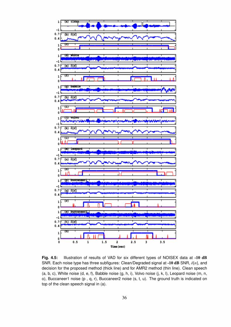
Fig. 4.5: Illustration of results of VAD for six different types of NOISEX data at -10 dB

SNR. Each noise type has three subfigures: Clean/Degraded signal at -10 dB SNR, δ[n], and

decision for the proposed method (thick line) and for AMR2 method (thin line). Clean speech

(a, b, c), White noise (d, e, f), Babble noise (g, h, i), Volvo noise (j, k, l), Leopard noise (m, n,

o), Buccaneer1 noise (p , q, r), Buccaneer2 noise (s, t, u). The ground truth is indicated on

top of the clean speech signal in (a).

36

Fig. 4.6: Illustration of results of VAD for six different types of NOISEX data at 5 dB SNR.

Each noise type has three subfigures: Clean/Degraded signal at 5 dB SNR, δ[n], and decision

for the proposed method (thick line) and for AMR2 method (thin line). Clean speech (a, b, c),

White noise (d, e, f), Babble noise (g, h, i), Volvo noise (j, k, l), Leopard noise (m, n, o),

Buccaneer1 noise (p, q, r), Buccaneer2 noise (s, t, u). The ground truth is indicated on top of

the clean speech signal in (a).

37

Fig. 4.7: Illustration of results of VAD for seven different types of NOISEX data at -10 dB SNR.

Each noise type has three subfigures: Degraded signal at -10 dB SNR, δ[n], and decision

for the proposed method (thick line) and for AMR2 method (thin line). Pink noise (a, b, c),

Hfchannel noise (d, e, f), m109 noise (g, h, i), f16 noise (j, k, l), Factory1 noise (m, n, o),

Factory2 noise (p, q, r), Machine gun noise (s, t, u). The ground truth is indicated on top of

the degraded speech signal in (a).

38

Fig. 4.8: Illustration of results of VAD for seven different types of NOISEX data at 5 dB SNR.

Each noise type has three subfigures: Degraded signal at 5 dB SNR, δ[n], and decision for the

proposed method (thick line) and for AMR2 method (thin line). Pink noise (a, b, c), Hfchannel

noise (d, e, f), m109 noise (g, h, i), f16 noise (j, k, l), Factory1 noise (m, n, o), Factory2 noise

(p, q, r), Machine gun noise (s, t, u). The ground truth is indicated on top of the degraded

speech signal in (a).

39

4.4.2 Performance on NTIMIT and CTIMIT databases.

Performance of the proposed method is similar to the AMR2 method for the NTIMIT

data (Table 4.4), and is higher than for the CTIMIT data (Table 4.4). This may be due

to the cellphone (coding) effects, which degrade speech more than the telephone channel

(NTIMIT). The lw value is 200 msec for most of the utterances in these cases because of

high ρ value (see (4.6)).

Table 4.4: Evaluation results of NTIMIT and CTIMIT database for the proposed method (PM)

in comparison with AMR2 method.

DATA METHOD CORRECT FEC MSC OVER NDS

NTIMIT PM 94.78 0.02 1.66 0.18 3.18

AMR2 93.59 0.12 2.91 0.21 2.91

CTIMIT PM 91.14 0.04 4.21 0.15 4.31

AMR2 87.68 0.15 8.28 0.19 3.46

4.4.3 Performance on distant speech.

-1

-0.5

0

0.5

1

1.5

(a) Close speaking speech (C0)

0.2

0.4

0.6

(b) [n]

0 0.5 1 1.5 2 2.5 3 3.5 4 Time(sec)

0

0.5

1

(c)

Fig. 4.9: (a) Distance speech (C0) with ground truth indicated on top. (b) δ[n]. (c) Decision of

the proposed method at η = 90% (solid line) and the AMR2 method (dotted line).

40

-1

-0.5

0

0.5

1

1.5(a) Distance speech (C3)

0.3

0.4

0.5 (b) [n]

0 0.5 1 1.5 2 2.5 3 3.5 4 Time(sec)

0

0.5

1

(c)

Fig. 4.10: (a) Distance speech (C3) with ground truth indicated on top. (b) δ[n]. (c) Decision

of the proposed method at η = 90% (solid line) and the AMR2 method (dotted line).

Distant speech is an amalgam of unknown degradations, and the data available for

a given environment may be limited. The reverberation present in the distant speech

signals has high variance in the time domain, as does the speech. So VAD methods often

confuse reverberation component for speech. The VAD methods which bank on temporal

variance ( [11] ) may not perform well, because the distant speech is highly nonstationary,

and even the nonspeech regions may have significant temporal variance.

Fig. 4.9 illustrates the decision obtained by the proposed method and by the AMR2

method for the case of close speaking speech (C0). The errors in the AMR2 method

and the proposed method are mostly due to FA (Fig. 4.9(c)). Note that the δ[n] values

(Fig. 4.9(b)) have large fluctuations in the speech region, and also it has low floor values

as for any clean speech. It is to be noted, that for distant microphone case the performance

of the proposed method gives results similar to the AMR2 method, indicating that the

proposed method does not fail. Table 4.5 indicates that by proper choice of the value

of the η parameter, there can be slight improvement. But the improvement may not be

significant. The interesting aspect is that most of the errors in this case are due to false

acceptance (FA). This occurs because the degradation in silence regions is not uniform in

the case of distant speech, making it difficult to set proper threshold either in the proposed

method or in the AMR2 method. One would notice larger fluctuations in the values of δ[n]

41

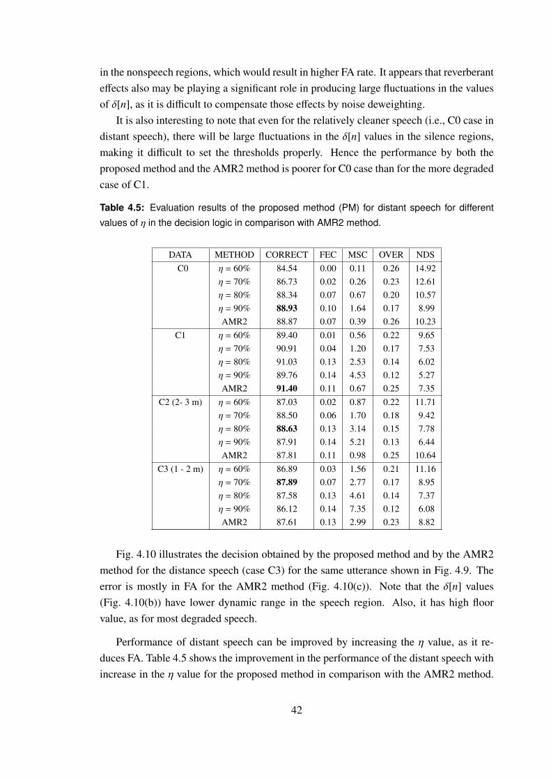
in the nonspeech regions, which would result in higher FA rate. It appears that reverberant

effects also may be playing a significant role in producing large fluctuations in the values

of δ[n], as it is difficult to compensate those effects by noise deweighting.

It is also interesting to note that even for the relatively cleaner speech (i.e., C0 case in

distant speech), there will be large fluctuations in the δ[n] values in the silence regions,

making it difficult to set the thresholds properly. Hence the performance by both the

proposed method and the AMR2 method is poorer for C0 case than for the more degraded

case of C1.

Table 4.5: Evaluation results of the proposed method (PM) for distant speech for different

values of η in the decision logic in comparison with AMR2 method.

DATA METHOD CORRECT FEC MSC OVER NDS

C0 η = 60% 84.54 0.00 0.11 0.26 14.92

η = 70% 86.73 0.02 0.26 0.23 12.61

η = 80% 88.34 0.07 0.67 0.20 10.57

η = 90% 88.93 0.10 1.64 0.17 8.99

AMR2 88.87 0.07 0.39 0.26 10.23

C1 η = 60% 89.40 0.01 0.56 0.22 9.65

η = 70% 90.91 0.04 1.20 0.17 7.53

η = 80% 91.03 0.13 2.53 0.14 6.02

η = 90% 89.76 0.14 4.53 0.12 5.27

AMR2 91.40 0.11 0.67 0.25 7.35

C2 (2- 3 m) η = 60% 87.03 0.02 0.87 0.22 11.71

η = 70% 88.50 0.06 1.70 0.18 9.42

η = 80% 88.63 0.13 3.14 0.15 7.78

η = 90% 87.91 0.14 5.21 0.13 6.44

AMR2 87.81 0.11 0.98 0.25 10.64

C3 (1 - 2 m) η = 60% 86.89 0.03 1.56 0.21 11.16

η = 70% 87.89 0.07 2.77 0.17 8.95

η = 80% 87.58 0.13 4.61 0.14 7.37

η = 90% 86.12 0.14 7.35 0.12 6.08

AMR2 87.61 0.13 2.99 0.23 8.82

Fig. 4.10 illustrates the decision obtained by the proposed method and by the AMR2

method for the distance speech (case C3) for the same utterance shown in Fig. 4.9. The

error is mostly in FA for the AMR2 method (Fig. 4.10(c)). Note that the δ[n] values

(Fig. 4.10(b)) have lower dynamic range in the speech region. Also, it has high floor

value, as for most degraded speech.

Performance of distant speech can be improved by increasing the η value, as it re-

duces FA. Table 4.5 shows the improvement in the performance of the distant speech with

increase in the η value for the proposed method in comparison with the AMR2 method.

42

Note that the large values of η can also cause increase in the true rejection (TR), which

may result in overall reduction in correct decision.

4.4.4 Performance on TIMIT database for clean speech.

Performance of the proposed method on clean speech is given in Table 4.6. It is interesting

to note that smoothing and threshold logic for degraded speech smear the information

across time, thus reducing the temporal resolution of the final decision. Hence when the

decision logic is applied to clean data, it appears to give poor performance. Due to the

high dynamic range in both time and frequency domains, the clean speech signal needs to

be treated differently in order to obtain good performance.

In contrast to the C0 case of distant speech, for the clean TIMIT data, the error is more

in the true rejection (TR) as in Table 4.6. This is because for the clean TIMIT data in the

silence region, the δ[n] values aa are very low and are fluctuating, making it difficult to set

the proper threshold. In this case the TR can be reduced by reducing the threshold value,

or equivalently reducing the η value.

Performance improved for the AMR2 method for clean and distance speech cases

compared to the proposed method (for the fixed η = 60%). This emphasizes the need

to incorporate several features corresponding to source and other supra-segmental level

features to improve the performance for the proposed method, without having to rely on

any parameter.

Table 4.6: Evaluation results of the proposed method (PM) for TIMIT clean case for different

values of η in the decision logic in comparison with AMR2 method.

η CORRECT FEC MSC OVER NDS

η = 40% 95.72 0.02 2.71 0.06 1.37

η = 50% 94.92 0.05 3.96 0.06 0.92

η = 60% 93.55 0.07 5.61 0.04 0.62

η = 70% 91.66 0.08 7.66 0.04 0.46

η = 80% 89.42 0.09 10.01 0.03 0.35

AMR2 93.59 0.12 2.91 0.21 2.91

4.5 Performance for varied values of the parameters θ,

lw, η

Tables 4.5 - 4.6 show the variation in performance with change in values for parameter η.

A better performance is also achieved when the other parameters θ or lw are adapted suit-

43

ably for each type of degradation. For example, the threshold (θ = µθ + 3σθ) fixed based

on mean (µθ) and variance (σθ) of the lower 20% of the δ[n] values of the utterance need

not be the threshold for the best performance in each case. In this section, the adaptation

criteria is explored based on the values chosen for θ, lw, η. Some VAD methods report

the performance for the best threshold [11], [28]. Tables 4.7 - 4.9 report the performance

for different values of θ, lw, η for a speech utterance degraded by different noises at SNR

of -10 dB. The performance in the tables has been reported with change for a specific

parameter while keeping the values for the other parameters constant with the values de-

termined by the decision logic. For example θ value is varied with fixed values for lw and

η.

Table 4.7: Results for the proposed method on TIMIT database for varied values of thresholds

(θ) across different noises.

NOISE CORRECT TR FA

θ = µθ + 2σθ white 80.00 1.12 18.88

f16 73.11 4.02 22.73

volvo 74.31 0.00 25.53

θ = µθ + 3σθ white 81.92 0.16 18.08

f16 62.31 36.93 0.37

volvo 95.41 0.00 4.43

θ = µθ + 5σθ white 79.52 20.48 0.00

f16 54.02 45.72 0.00

volvo 99.08 0.00 0.76

Table 4.8: Results for the proposed method on TIMIT database for varied values of lw across

different noises.

NOISE CORRECT TR FA

lw = 200 msec white 81.92 18.08 0.00

f16 57.53 42.20 0.01

volvo 99.08 0.00 0.76

lw = 400 msec white 84.48 15.52 0.00

f16 62.31 36.93 0.37

volvo 96.94 0.00 2.90

lw = 600 msec white 87.32 12.68 0.00

f16 61.80 37.93 0.01

volvo 94.34 0.00 5.50

44

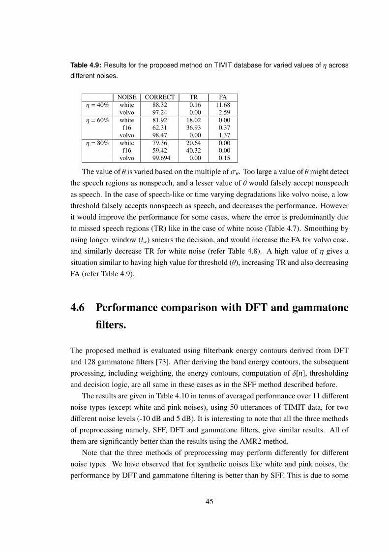
Table 4.9: Results for the proposed method on TIMIT database for varied values of η across

different noises.

NOISE CORRECT TR FA

η = 40% white 88.32 0.16 11.68

volvo 97.24 0.00 2.59

η = 60% white 81.92 18.02 0.00

f16 62.31 36.93 0.37

volvo 98.47 0.00 1.37

η = 80% white 79.36 20.64 0.00

f16 59.42 40.32 0.00

volvo 99.694 0.00 0.15

The value of θ is varied based on the multiple ofσθ. Too large a value of θmight detect

the speech regions as nonspeech, and a lesser value of θ would falsely accept nonspeech

as speech. In the case of speech-like or time varying degradations like volvo noise, a low

threshold falsely accepts nonspeech as speech, and decreases the performance. However

it would improve the performance for some cases, where the error is predominantly due

to missed speech regions (TR) like in the case of white noise (Table 4.7). Smoothing by

using longer window (lw) smears the decision, and would increase the FA for volvo case,

and similarly decrease TR for white noise (refer Table 4.8). A high value of η gives a

situation similar to having high value for threshold (θ), increasing TR and also decreasing

FA (refer Table 4.9).

4.6 Performance comparison with DFT and gammatone

filters.

The proposed method is evaluated using filterbank energy contours derived from DFT

and 128 gammatone filters [73]. After deriving the band energy contours, the subsequent

processing, including weighting, the energy contours, computation of δ[n], thresholding

and decision logic, are all same in these cases as in the SFF method described before.

The results are given in Table 4.10 in terms of averaged performance over 11 different

noise types (except white and pink noises), using 50 utterances of TIMIT data, for two

different noise levels (-10 dB and 5 dB). It is interesting to note that all the three methods

of preprocessing namely, SFF, DFT and gammatone filters, give similar results. All of

them are significantly better than the results using the AMR2 method.

Note that the three methods of preprocessing may perform differently for different

noise types. We have observed that for synthetic noises like white and pink noises, the

performance by DFT and gammatone filtering is better than by SFF. This is due to some

45

temporal and spectral averaging of noises in the high frequency region (> 2000 Hz) due

to temporal averaging in the case of DFT and due to spectral smoothing in the case of

gammatone filters. The performance imprperform ovement for all the three methods will

be similar even for these two types of noises, if in the SFF method some smoothing is

done in the time and frequency domains, especially in the higher frequency region, before

computing mean and variance across frequency. Also note that though the features from

DFT and gammatone filtering worked for speech detection, they were unable to perform

in other tasks namely, transient noise detection, estimation of fundamental frequency ( fo)

and glottal closure instants, due to their respective temporal and spectral averaging effects.

Table 4.10: Averaged scores using features from different methods across all noise types for

two SNR levels for TIMIT database.

SNR (dB) METHOD CORRECT FEC MSC OVER NDS

-10 SFF 81.25 0.05 12.36 0.03 6.20

DFT 81.69 0.02 4.31 0.06 13.83

Gammatone 81.63 0.06 11.98 0.03 6.20

AMR2 74.63 0.06 15.19 0.05 9.94

5 SFF 94.77 0.02 2.37 0.05 2.68

DFT 93.38 0.01 1.12 0.06 5.33

Gammatone 93.24 0.03 3.78 0.03 2.82

AMR2 88.75 0.04 1.52 0.09 9.46

Note that the performance improvement of these three preprocessing methods over the

AMR2 method is due to the subsequent processing of the energy contours in each band,

especially the weighting in (4.1). The effect of weighting can be seen in the performance

of the proposed method with and without weighting as given in Table 4.11. The average

scores across all noise types for two different SNR values (-10 dB and 5 dB) are given

using unweighted and weighted SFF output for 50 utterances of TIMIT data.

Table 4.11: Averaged scores across all noise types for two SNR levels of unweighted and

weighted SFF output for TIMIT database.

SNR (dB) METHOD CORRECT FEC MSC OVER NDS

−10 Unweighted SFF 70.73 0.07 19.45 0.03 9.60

Weighted SFF 78.04 0.07 15.82 0.03 5.94

5 Unweighted SFF 93.18 0.03 3.80 0.05 2.83

Weighted SFF 95.15 0.02 2.25 0.06 2.41

46

4.7 Performance comparison with LTSV method.

In the case of LTSV method proposed in [11], there is requirement of prior training data

to estimate the information about noise characteristics and SNR. Also LTSV method as-

sumes nonspeech beginning in the initial 2 sec duration from which the thresholds are

initiated. The method relied on long term features and uses a frame size of 300 msec, so it

can not work for a short duration speech utterance. A VAD method should work for short

durations also. The proposed method does not have such constraints or limitations. Other

VAD methods did not consider the wide variety of NOISEX noises as in [11]. The pro-

posed method also evaluated for practical degradations such as NTIMIT, CTIMIT, distant

speech.

The long term spectral variability (LTSV) method gave the performance after aver-

aging the scored across several SNRs, except for SNR = -10 dB. Processing information

over more duration would reduce the effect of noise for lower SNR cases as noise power

gets reduced when averaged across long duration. However for the higher SNR cases,

processing information over long frames may also spread speech characteristics into its

neighbouring nonspeech regions and vice versa, thereby decreasing accuracy. Ideally,

a VAD method is supposed to work independent of SNR. Here the comparison of LTSV

method and the proposed method is done through the AMR2 method, as both the methods

have reported performance of AMR2 method. It is observed that the LTSV method per-

formed poorly compared to AMR2 method in the cases of colored, high time-varying and

speech-like noises, i.e., pink, military vehicle (leopard), car interior (volvo) and babble, as

evident from the of averaged CORRECT score across SNRs [11]. At SNR = -10 dB, the

AMR2 method performed better than the LTSV method for military vehicle, car interior,

machine gun and babble noises. The proposed method performed better than the AMR2

method for all these cases, also indicating a better performance in comparison to LTSV

method. The poor performance of the LTSV method in the cases of colored, high time-

varying and speech-like noises is due to high false acceptance (FA). Hence, it is likely

that the LTSV method may not perform well for distant speech as reverberation effects in

distant speech often confuse nonspeech with speech.

4.8 Summary

A new VAD method is proposed based on single frequency filtering (SFF) method in

this chapter. The method exploits the fact that speech has high SNR regions at different

frequencies and at different times. The variance of speech across frequency is higher

than that for noise, after compensating for spectral characteristics for noise. The spectral

47

characteristics of noise are determined using the floor of the temporal envelope at each

frequency, computed by the SFF method.

The δ[n] feature proposed for VAD decision is robust against degradation, as evi-

denced by the high CORRECT percentage scores obtained for all types of noises. The

proposed method is tested over standard TIMIT, NTIMIT and CTIMIT databases, as well

as for distance speech, thus covering varieties of degradations. While the results show

significant improvement in performance of the proposed method, in comparison with the

AMR2 method, better results may be obtained, if the decision logic parameters (θ, η,

lw) are made degradation-specific. It was noticed that adapting the parameters θ, η, lw

based on the degradation characteristics estimated from ρ has improved the overall per-

formance. Adapting the threshold with time in each utterance may also improve the per-

formance. Further improvement can be expected if other characteristics of speech, such

as voicing, are also included in the decision logic. Also the δ[n] feature is not robust for

speech degraded by transient noises, as they exhibit high δ[n] values similar to speech. In

the next chapter, new features are developed for such noises exploiting the instantaneous

characteristics of speech derived using SFF method.

48

Chapter 5

Speech detection in transient noises

Voice activity detection (VAD) systems mentioned in the literature do not perform well in

transient noise degradation. Features derived using traditional methods are not adequate

for VAD in the case of transient noises. Transient noises are sounds of impulsive nature

occupying several frequency bands. Features like spectral energies, spectral variance and

temporal variance exhibit high values for transient noise similar to speech, thereby mak-

ing transient noise get accepted as speech. Some VAD methods attempted detection of

transient noises by training statistical models for each type of transient noise. There are

a variety of transient noises occurring generally, and training for each type of transient

noise is not possible.

The method proposed in this chapter exploits the impulse-like characteristics of the

transient noises to detect and suppress its effects in the speech degraded by such noises. A

time varying threshold (θt) is determined from the temporal changes in the spectral vari-

ance values computed over a small duration to discriminate transient noise from speech.

Notice that the method requires instantaneous features which are derived using single fre-

quency filtering method, as the speech characteristics derived by the block-based methods

smooth out the temporal changes, and the threshold is not estimated properly. The pro-

posed method is an unsupervised method, and does not require any prior information like

data for training or about the type of transient noise. The method is tested for several

types of transient noises, and it performed significantly better compared to the state-of-art

AMR methods. The periodicity information derived from the compensated envelopes is

also exploited for VAD across degradations, without being constrained to transient noises.

Section 5.1 gives the development of the proposed VAD method for transient noises.

In section 5.2, the database of different types of transient noises is discussed. In sec-

tion 5.3, the performance of the proposed VAD method is compared with AMR methods.

In section 5.4 a VAD method is developed which adapts for transient noises as well as

49

other noise scenarios. Section 5.5 gives the performance of the method. Section 5.6 gives

a summary of the study.

5.1 Proposed VAD method for transient noises

5.1.1 Detection of transient regions

0 0.5 1 1.5 2 2.5 3 3.5−1

0

1(a) Clean speech signal

0 0.5 1 1.5 2 2.5 3 3.5−1

0

1(b) Degraded signal

0 0.5 1 1.5 2 2.5 3 3.50

0.5

1

1.5

2

2.5

3

Time(sec)

(c)σ[n]

θt[n]

Fig. 5.1: (a) Clean speech signal. (b) Speech signal corrupted by door knock noise. (c) Values of σ[n] (bold

line) and θt[n] (dashed line).

The amplitude envelopes (ek[n]) are computed at intervals of 20 Hz in the frequency

range from 0 Hz to 4000 Hz. The value of standard deviation (σ[n]) is computed at each

time instant across frequencies of the envelopes. Fig. 5.1 shows the clean speech, de-

graded speech, and the values of spectral deviation (σ[n]) and the time varying threshold

(θt[n]) for speech signal degraded with door knock noise. It is observed that the σ[n]

values are high for speech and also for transient noise (Fig. 5.1(c)), as they exhibit a wide

range of spectrum with a high dynamic range. So the δ[n] feature proposed for VAD de-

cision in the previous chapter does not discriminate speech from transient noise well. The

50

standard deviation (σt[n]) of σ[n] values computed over a short duration (10 msec) is high

for transient noise due to its abrupt change. A time varying threshold (θt[n]) is computed

as twice of σt[n]. After experimentation the θt[n] is fixed as twice of σt[n], as a higher

value θt[n] (θt[n] = 3σt[n]) was observed to miss the speech regions, and a lower value

θt[n] (θt[n] = σt[n]) was not able to detect transient noise. For different speech sounds, it

is observed that the values of θt[n] are always lower than the σ[n] values (Fig. 5.1(c)). For

the transient noise, the values of θt[n] are higher than the σ[n] values, except near the peak

of the transient (Fig. 5.1(c)). Transient affected regions are detected by their σ[n] values

being less than their θt[n] values. The speech signal is further processed after detection of

the transient regions for VAD decision as discussed in the next section.

5.1.2 Detection of the nontransient nonspeech regions

Histogram of σ[n] values computed over an utterance is used to discriminate the speech

from nonspeech regions. The histogram is computed for σ[n] values with 400 bins. The

peak in the histogram would indicate the nonspeech threshold (θns). Speech regions where

(σ[n] ≤ θns) are considered as nonspeech.

The AMR methods would accept transient effected speech regions as speech due to the

high temporal variance characteristic of the transient noise, rather than due to the speech

characteristics. In the proposed method some low SNR speech regions affected by tran-

sient noise might be attenuated, as the method may detect the speech regions as transient

noise, leading to loss of speech. The loss of speech regions depends on the frequency

of occurrence of the transient noise. In order to get the lost speech regions, a hangover

technique is applied (as was done in [11], [16]). If at least 30% of the regions in the

neighbourhood of 400 msec is speech, then accept that frame as speech, else nonspeech.

5.2 Database

The utterances are taken from TIMIT TEST corpus. A subset of 84 utterances are con-

sidered from the total of 1680 (as done in [28]). Each utterance is of a different speaker

and of a different sentence. Half of them are male speakers and rest of them are female

speakers. Different samples of machine gun noise are taken from NOISEX database [75].

The other noise samples are taken from the website freesound.org. Sometimes the length

of the transient noise may not match the length of the speech signal. In such a scenario,

the whole of transient noise is repeated to match the length of the speech signal. Vari-

ous sounds of paper wrapping, keyboard typing, door knock, metronome, key dropping,

51

door slam, laptop keyboard typing, door knock with a door knocker, desk thump are con-

sidered. The VAD method should be tested for both speech acceptance and nonspeech

rejection. This requires similar ratios of speech and nonspeech data. So each TIMIT ut-

terance is added with 2 sec of silence at the beginning and end of the utterance as was

done in [11]. The ground truth is derived from the TIMIT phone labels. The proposed

method is compared with state-of-the-art AMR1 and AMR2 methods [14]. The transient

noises are normalized to the maximum of speech utterance amplitude and then added as

was done in [24], [28]. The parameters for the evaluation of the VAD methods were

discussed in section 4.3.

5.3 Performance of the proposed method for VAD in tran-

sient noises

Table 5.1 shows the performance of the proposed VAD method (PM) along with the AMR

methods for various transient noises. The best performance in each case is indicated by

bold face. It can be observed from Table 5.1 that there is significant reduction in FA (i.e.,

OVER + NDS) for the proposed method due to the attenuation of the transient noise. The

AMR methods give high FA. This implies that they are not able to discriminate transient

noise from speech. The low TR of the AMR methods is due to the transient noise accepted

as speech.

The work in [28] report the CORRECT score for VAD as well as the percentage

of transient noise detected. The CORRECT score depends on the proportion of speech

and nonspeech regions in the analysed data, which is different in our method. Hence

we use only the percentage of transient regions detected in our method for comparison.

For keyboard typing noise, the number of transient detected by our method is 97.97%,

whereas the number of transients detected by the method in [28] is 68.53%, and by the

AMR2 method is 5%. For metronome noise, the number of transients detected by the

proposed method and method in [28] are 97.53% and 75.96%, respectively, and 5.18%

for AMR2 . Moreover, the method in [28] is supervised and the results are reported for the

best threshold. Our method is unsupervised and uses an automatic time varying threshold.

The method in [11] reports CORRECT values giving similar performance as AMR2 for

machine gun noise, whereas our method gives 85.49% which is 18.4% better than the

AMR2 score.

Some studies reported methods suitable for a particular type of transient noise [24],

[27], [28], [29]. The proposed method is similar across different transient noises. Also,

the proposed method does not use statistical models for VAD, unlike many other methods.

52

Table 5.1: Evaluation results for the proposed method (PM) and AMR methods for different

transient noises.

TRANSIENT NOISE METHOD CORRECT FEC MSC OVER NDS

paper wrapping PM 80.46 0.08 6.10 0.10 13.09

AMR2 54.76 0.01 0.16 0.12 44.84

AMR1 51.05 0.00 0.10 0.12 48.61

keyboard typing PM 82.72 0.08 7.21 0.10 9.73

AMR2 75.46 0.01 0.37 0.11 23.95

AMR1 74.57 0.00 0.52 0.12 24.67

knocking on door PM 81.34 0.06 3.18 0.11 15.13

AMR2 57.11 0.00 0.19 0.12 42.48

AMR1 53.13 0.00 0.23 0.12 46.41

metronome PM 87.48 0.09 10.82 0.09 1.36

AMR2 74.80 0.01 0.38 0.11 24.60

AMR1 71.60 0.01 0.22 0.12 27.95

key drop PM 84.33 0.09 7.94 0.10 7.37

AMR2 74.49 0.01 0.34 0.11 24.94

AMR1 73.95 0.00 0.51 0.12 25.31

door slam PM 86.13 0.08 11.29 0.09 2.24

AMR2 80.08 0.01 0.49 0.11 19.21

AMR1 77.74 0.00 0.34 0.12 21.69

laptop keyboard typing PM 90.50 0.09 7.27 0.10 1.86

AMR2 46.19 0.00 0.06 0.12 53.51

AMR1 43.52 0.00 0.00 0.12 56.25

door knocker knock PM 88.61 0.09 9.55 0.09 1.48

AMR2 76.64 0.00 0.38 0.12 22.75

AMR1 74.46 0.00 0.26 0.12 25.06

desk thump PM 91.55 0.09 5.87 0.10 2.20

AMR2 51.20 0.00 0.12 0.12 48.45

AMR1 47.14 0.00 0.11 0.12 52.52

machine gun PM 85.49 0.07 5.01 0.11 9.14

AMR2 67.01 0.01 0.37 0.12 32.37

AMR1 63.46 0.01 0.48 0.12 35.82

5.4 Proposed VAD method exploiting the strength of pe-

riodicity from degraded speech

A time varying threshold is determined from instantaneous spectral values for detection

of transient noise. There is still a need for a VAD method unified across transient noises

as well as other noises. The periodicity information of the speech signal derived from

53

the instantaneous spectral variance values is explored for this purpose. The peak ampli-

tude derived from the autocorrelation sequence of the differenced spectral variance values

indicate the strength of periodicity, and is used for VAD.

(a) Clean speech signal

0 1 2 3 4 5 6 7−1

−0.5

0

0.5

1

1.5

(b) Degraded signal

0 1 2 3 4 5 6 7−1

0

1

0 1 2 3 4 5 6 70

0.00002

0.00004

(c) Spectral variance (σ2[n])

0 1 2 3 4 5 6 7−0.000005

0

0.000005

(d) Differenced signal (σd

2[n])

0 1 2 3 4 5 6 70

0.5

1

Time (sec)

(e) Normalised peak amplitude

Fig. 5.2: (a) Clean speech signal. (b) Degraded speech signal corrupted by desk thump

noise at 0 dB SNR. (c) Variance (σ2[n]). (d) Differenced signal (σ2d[n]). (e) Normalized peak

amplitude.

The mean of lower 20% values of envelopes ek[n] at each frequency fk are used to

derived weight values wk. That is

wk =

1µk∑N

l=11µl

, (5.1)

The weighted envelopes ck[n] are computed as

ck[n] = wkek[n]. (5.2)

The spectral variance (σ2[n]) derived from the weighted envelopes is differenced to give

54

the differenced signal (σ2d[n]). Autocorrelation function is applied on the σ2

d[n] values

using a frame size of 30 msec and frame shift of 1 msec. The maximum peak amplitude

of the normalized AC sequence in the range of 2 - 15 msec is considered for every frame.

The peak amplitudes are smoothed over 200 msec, and a threshold of 0.3 is applied

on the smoothed values.

A hangover technique is applied so that if at least 60% of the regions in the neigh-

bourhood of 400 msec is speech, then accept that frame as speech, else nonspeech.

Fig. 5.3: (a) Clean speech signal. (b) Degraded speech signal corrupted by white noise at at

0 dB SNR. (c) Variance (σ2[n]). (d) Differenced signal (σ2d[n]). (e) Normalized peak amplitude.

Figs. 5.2 and 5.3 show the values of variance (σ2[n]), differenced signal (σ2d[n]) along

with normalized peak amplitudes for speech degraded with transient noise and white noise

at SNR of 0 dB, respectively. Notice that for transient noise, values of both variance

(σ2[n]) and differenced signal (σ2d[n]) are high, similar to speech (Figs. 5.2(c), 5.2(d)).

However, the normalized peak amplitude is less for transient noise. Transient noise af-

fected speech regions, on the other hand, still have high peak amplitudes due to speech

55

characteristics (Fig. 5.2(e)). For white noise degraded speech, the values of variance

(σ2[n]), differenced signal (σ2d[n]) and normalized peak amplitudes are all low in non-

speech regions compared to speech regions (Fig. 5.3).

Speech characteristics got enhanced after compensating for noise, and the instanta-

neous characteristics derived by the SFF method are able to preserve the pitch period

fluctuations. So the AC sequences derived from the differenced variance (σ2d[n]) showed

better evidence compared to the AC sequences computed from the degraded speech sig-

nal. On the other hand, the normalized peak amplitudes derived from the AC sequences

of the degraded speech signal did not show much evidence as they were affected by the

degradation characteristics. The AC sequences derived from the transient noise signal

also had high peak amplitude due to their low frequency content. Notice that speech fea-

tures computed using block-based parameters like DFTs and MFCCs average the spectral

information across the block (frame), and can not preserve the finer pitch period based

fluctuations.

5.5 Performance of the proposed VAD method

Table 5.2 shows the performance of the proposed method (PM2) and AMR methods

across various noises. The noises were added at SNR of 0 dB. The error for the transient

noise degradations lie mostly in false acceptance (FA) for the transient effected speech for

the AMR methods as their impulsive nature often gets confused with speech.

Notice that the proposed method (PM2) performed high even for other degradations

of white, babble and volvo cases [75]. The FA decreased for the proposed method even

in the case of time varying volvo and babble noises, as the proposed method relied on

the periodicity information and not on the spectral energies. The proposed method (PM2)

does not break down for transient noises unlike the AMR methods. Also, methods in

the literature deal exclusively for transient noises, training for each transient noise and

for each SNR separately [24], [28], [29]. Estimation of threshold usually has issues as

it has to vary with SNR and noise levels, and sometimes the given utterance may only

have nonspeech. In such scenarios it is relevant that we have a fixed threshold exploiting

some characteristics of speech apart from energy levels of speech or noise. The proposed

method method uses a fixed threshold exploiting the periodicity characteristics of speech

across different noises and at different SNR levels. The method did not perform well

at low SNRs of -10 dB SNR, as the pitch period information was lost. The performance

56

Table 5.2: Evaluation results for the proposed VAD method (PM2) and AMR methods across

NOISEX noises and transient noises.

NOISE METHOD CORRECT FEC MSC OVER NDS

keyboard typing PM2 90.57 0.11 8.35 0.03 0.78

AMR2 49.10 0.01 0.62 0.03 50.05

AMR1 47.74 0.02 0.04 0.01 51.96

desk thump PM2 81.95 0.05 0.22 0.05 17.51

AMR2 65.69 0.01 0.02 0.02 34.04

AMR1 62.01 0.00 0.00 0.01 37.76

key drop PM2 95.83 0.11 3.14 0.03 0.67

AMR2 71.92 0.01 0.04 0.01 27.79

AMR1 73.01 0.01 0.10 0.04 26.62

machine gun PM2 91.71 0.05 1.79 0.05 6.18

AMR2 68.56 0.05 0.49 0.05 30.62

AMR1 68.40 0.05 0.49 0.05 30.79

white PM2 91.07 0.16 8.01 0.03 0.35

AMR2 87.43 0.15 11.93 0.01 0.37

AMR1 83.14 0.11 3.79 0.05 12.68

volvo PM2 97.23 0.16 7.39 0.02 0.08

AMR2 95.01 0.02 0.52 0.02 4.26

AMR1 91.65 0.05 0.16 0.05 7.86

babble PM2 83.28 0.11 16.40 0.01 0.04

AMR2 79.35 0.08 7.83 0.11 12.46

AMR1 61.08 0.06 0.48 0.04 38.09

would improve by considering several features like the AMR methods using a hierarchical

decision logic.

5.6 Summary

In this chapter, methods are proposed for VAD for speech corrupted by transient noises.

The characteristics of speech present at each sample are exploited using the instantaneous

features derived from the single frequency filtering method. The features at instantaneous

level are able to discriminate transient noises from speech. The spectral variance feature is

exploited in different ways to detect the transient noise. Notice that the methods proposed

work for different types of transient noises, unlike other methods proposed for transient

noise detection. In this chapter, the importance of developing VAD methods which do

not require to deal separately with transient degradations and other degradations is high-

lighted. The periodicity information is exploited using the spectral variance feature for

this purpose. The correlation sequence derived from the noise-compensated envelopes

showed evidence of periodicity in the degraded speech, which was lost in the correlation

57

sequence computed from the degraded speech. Notice that unlike the other VAD methods

the proposed method does not have any threshold estimation, as it uses a fixed threshold

based on periodicity information, and hence can be adapted to real environments. This

envisions to develop VAD methods based on various features and integrate them at a hi-

erarchical level, similar to the AMR methods, where several features are implemented in

a decision-based manner.

58

Chapter 6

Extraction of fundamental frequency

from degraded speech

Voiced speech is produced due to excitation caused by the vibration of vocal folds. The

pitch period (to) is the time interval of each cycle of the vocal fold vibration. The funda-

mental frequency ( fo) or the rate of vibration of the vocal folds is the inverse of the pitch

period (to). The estimation of fo is affected not only by the interaction of the vocal folds

with the vocal tract system, but also by the degradations in the speech signal.

Methods for estimation of the fundamental frequency have been evaluated mainly for

simulated degradations, i.e., where samples of noise are added to the speech signal (eg

NOISEX degradations [75]) or speech filtered through degradation channel (eg cellphone

degradation). There have been fewer attempts for data collected in realistic scenarios,

where the types of degradation and background conditions vary, and are hard to estimate.

Distant speech collected in different environments is one such realistic scenario. It has

been observed that standard fo methods did not perform across different degradations,

including the distance speech. Note that in real environments, the speech may get af-

fected with multiple unknown degradations, including reverberation. Hence it is required

to develop methods for fo extraction that are independent of degradations. The correlation

sequences or harmonics derived from the speech signal are modified in several ways by

different methods to highlight the fo characteristics for its estimation. Methods have also

been proposed to exploit fo characteristics by filtering and processing information derived

at different frequency bands. These methods were not able to give a reliable performance

when affected with degradations. In this chapter, an fo estimation method is proposed

using the information derived at the most robust frequency for each frame, to overcome

the effects of degradations. In this chapter, the high signal-to-noise ratio (SNR) segments

of the speech signal at some frequencies derived using single frequency filtering (SFF)

59

method are exploited for fo extraction using autocorrelation function of those segments.

Since the fo is computed from the envelope of a single frequency component of the signal,

the vocal tract resonances do not affect the fo extraction. The use of the high SNR fre-

quency component in a given segment helps in overcoming the effects of degradations in

the speech signal, without explicitly estimating the characteristics of noise. The proposed

method for fo extraction was tested for both real and simulated degradations [81].

Section 6.1 discusses the modification of temporal and spectral resolutions of features

derived using single frequency filtering approach which form the basis of the proposed

method for fo estimation. Section 6.2 describes the proposed method for fo estimation

exploiting the high SNR feature of SFF outputs. In particular, the noise floor of the SFF

output is compensated using a weight function, and the fo is estimated from the dominant

frequency SFF envelope using autocorrelation of the envelope. Section 6.3 discusses the

issues in the evaluation of fo estimation methods for different degradations. In particular,

the databases, types of degradations, other fo estimation methods for comparison, and

parameters for evaluation of the fo estimation methods are described briefly in this section.

In section 6.4, performance of the proposed method is compared with the performance

of other standard methods for speech in different degradations. Section 6.5 discusses a

method proposed for f0 estimation with incorporation of voiced decisions required for

reliable f0 estimation for speech systems. The evaluation parameters, methods used for

comparison and their performance across various degradations are also discussed in this

section. Section 6.7 gives a summary of the chapter.

6.1 Features of SFF signals.

Note that the single frequency filter has a pole filter whose transfer function is given by

H(z) =1

1 + rz−1. (6.1)

The root of this filter is located on the real axis at z = −r in the z-plane, whose angle

corresponds to half the sampling frequency, i.e., fs/2. The output yk[n] for the speech

signal x[n] is given by [74]

yk[n] = −ryk[n − 1] + xk[n]. (6.2)

The envelope of the signal yk[n] is given by

ek[n] =√

ykr2[n] + yki

2[n], (6.3)

60

where ykr[n] and yki[n] are the real and imaginary components of yk[n]. The bandwidth of

the filter is controlled by the value of r. In fact, the value of r should be close to 1 if the

filter were to act as an ideal resonator at fs/2. For r close to 1, say r = 0.995, the output is

like a modulated signal with a carrier frequency of fs/2. The envelope of the component

signal is smeared in time, but gives a good frequency resolution, when the components

are obtained at different frequencies. When r is lower, say r = 0.95, the envelope of the

component signal will have higher temporal resolution (lesser smearing) compared to the

case of r = 0.995. The envelopes of a segment of speech signal at fk = 1000 Hz for

fs = 10 kHz, are given in Fig. 6.1, for the cases of r = 0.995 and r = 0.95. The figure

clearly shows the differences in the temporal resolution of the envelope features. The

spectral envelope obtained by collecting the values of the envelopes at a given instant for

different frequencies indicates higher frequency resolution for r = 0.995 (Fig. 6.1(d)) and

lower frequency resolution for r = 0.95 (Fig. 6.1(e)).

0 0.5 1 1.5 2 2.5 3−1

0

1(a) Clean speech signal

0 0.5 1 1.5 2 2.5 30

5

10(b) Envelopes derived at r = 0.995 at 1 kHz

0 0.5 1 1.5 2 2.5 30

2

4

Time (sec)

(c) Envelopes derived at r = 0.95 at 1 kHz

0 500 1000 1500 2000 2500 3000 3500 4000 4500 50000

10

20

freq (Hz)

(d) Spectral envelopes derived at r = 0.995

0 500 1000 1500 2000 2500 3000 3500 4000 4500 50000

2

4

freq (Hz)

(e) Spectral envelopes derived at r = 0.95

Fig. 6.1: (a) Clean speech signal. (b) Envelope at 1 kHz derived as a function of time for

r = 0.995. (c) Envelope at 1 kHz derived as a function of time for r = 0.95. (d) Spectral

envelope at t = 0.5 sec for r = 0.995. (e) Spectral envelope at t = 0.5 sec for r = 0.95.

The signal to noise power ratio of degraded speech signal is a function of time as

61

well as frequency. In the frequency domain the noise power gets distributed more evenly

compared to speech. Thus, the signal-to-noise ratio (SNR) depends on how the signal is

decomposed for further processing. Let us examine the SNR characteristics of the SFF

envelopes as a function of frequency. Let S ( f ) and N( f ) denote the spectral envelopes of

the degraded speech signal and noise as a function of frequency.

Let fD be the frequency at which the ratioS 2( f )

N2( f )is maximum in a given frame. A frame

of size 20 msec for every sample shift is used for computing the SNRs. Let us define the

following different cases of computing the SNR ratios:

αD =S 2( fD)

N2( fD), (6.4)

α =

∫ fL

f0

S 2( f )

N2( f )d f , (6.5)

β =

L−1∑

i=0

∫ fi+1

fiS 2( f ) d f

∫ fi+1

fiN2( f ) d f

, (6.6)

and

γ =

∫ fL

f0S 2( f ) d f

∫ fL

f0N2( f ) d f

, (6.7)

where ( fi − fi+1) is the (i + 1)th interval of the L nonoverlapping frequency bands, and

i = 0, 1, ..., L − 1 [74]. The following inequality holds good.

αD ≥ α ≥ β ≥ γ. (6.8)

The average SNR of the individual frequencies (α) is less compared to αD, because

the high SNR at FD is averaged with the lower SNRs at other frequencies. The SNR is re-

duced across subbands (β), because the power at the high SNR (robust) frequency is aver-

aged with those at the low SNR frequencies present in the subbands. The SNR computed

from the averaged power across all the frequencies (γ) is less because the average noise

power is used. The proposed method uses features at the dominant frequencies (FD) for

fo extraction. The spectral envelopes S ( f ) and N( f ) are computed for a degraded speech

utterance and for noise using the single frequency filtering (SFF) approach for frequencies

in the range of 0 - 4000 Hz using L = 16. The average values of αD, α, β and γ computed

over the entire utterance are denoted asαD, α, β and γ, respectively. These parameters are

computed for two different values of r, namely, r = 0.99 and r = 0.95, corresponding to

high (low) and low (high) frequency (temporal) resolution. The inequality in (6.8) holds

62

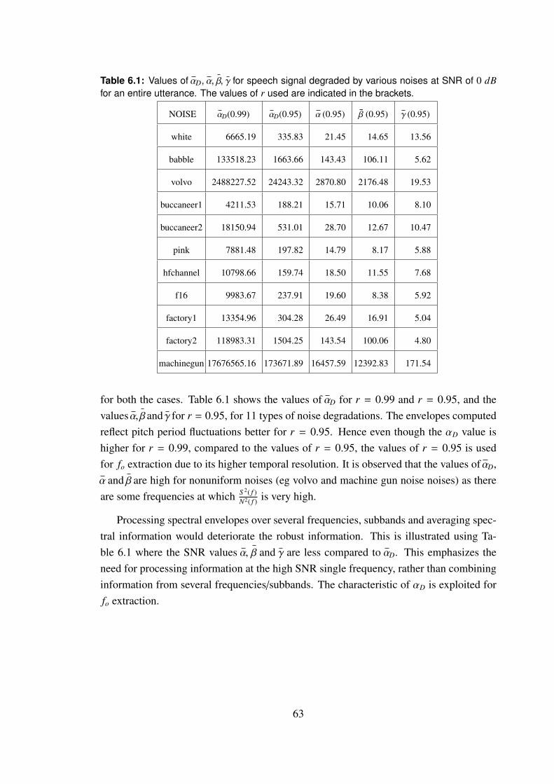
Table 6.1: Values of αD, α, β, γ for speech signal degraded by various noises at SNR of 0 dB

for an entire utterance. The values of r used are indicated in the brackets.

NOISE αD(0.99) αD(0.95) α (0.95) β (0.95) γ (0.95)

white 6665.19 335.83 21.45 14.65 13.56

babble 133518.23 1663.66 143.43 106.11 5.62

volvo 2488227.52 24243.32 2870.80 2176.48 19.53

buccaneer1 4211.53 188.21 15.71 10.06 8.10

buccaneer2 18150.94 531.01 28.70 12.67 10.47

pink 7881.48 197.82 14.79 8.17 5.88

hfchannel 10798.66 159.74 18.50 11.55 7.68

f16 9983.67 237.91 19.60 8.38 5.92

factory1 13354.96 304.28 26.49 16.91 5.04

factory2 118983.31 1504.25 143.54 100.06 4.80

machinegun 17676565.16 173671.89 16457.59 12392.83 171.54

for both the cases. Table 6.1 shows the values of αD for r = 0.99 and r = 0.95, and the

valuesα,βandγ for r = 0.95, for 11 types of noise degradations. The envelopes computed

reflect pitch period fluctuations better for r = 0.95. Hence even though the αD value is

higher for r = 0.99, compared to the values of r = 0.95, the values of r = 0.95 is used

for fo extraction due to its higher temporal resolution. It is observed that the values ofαD,

α and β are high for nonuniform noises (eg volvo and machine gun noise noises) as there

are some frequencies at whichS 2( f )

N2( f )is very high.

Processing spectral envelopes over several frequencies, subbands and averaging spec-

tral information would deteriorate the robust information. This is illustrated using Ta-

ble 6.1 where the SNR values α, β and γ are less compared to αD. This emphasizes the

need for processing information at the high SNR single frequency, rather than combining

information from several frequencies/subbands. The characteristic of αD is exploited for

fo extraction.

63

6.2 Proposed method for fo estimation.

The proposed method for fo estimation is termed as SFF method, and it exploits the

presence of high SNR regions in the SFF outputs of the input speech signal. The envelopes

of the SFF outputs at different frequencies are processed to compensate for the noise

floor caused by degradations in the speech signal. For each segment of speech signal,

the frequency of the highest SNR envelope among the processed envelopes at different

frequencies is considered as the dominant frequency (FD). The autocorrelation function

of the segment of the dominant frequency envelope is used for extracting fo.

6.2.1 Noise compensation of the SFF envelopes of degraded speech.

Let S k be the set of minimal 20% values of ek[n], then the average of the values in the set

is denoted by µk.

The normalized weight value for the envelope at fk is computed as [74]

wk =

1µk∑N

l=11µl

, (6.9)

where N is the number of frequencies at which the SFF envelopes are obtained. In the

current study, the SFF envelopes are obtained for every 20 Hz, and hence N = 200 in the

frequency range of 0 - 4000 Hz. The envelope ek[n] at fk is compensated for noise after

multiplication with the weight value wk. The weighted envelopes ck[n] are given by

ck[n] = wkek[n]. (6.10)

6.2.2 Determination of dominant frequencies (FD).

Frames (segments) of size 40 msec are considered using a frame shift of 5 msec for

estimation of fo. The frame energies are computed from the mean-subtracted envelopes

in each frame. The frame energies of the mean-subtracted envelopes are averaged over

adjacent 16 frames (corresponding to 80 msec for the 5 msec frame shift) to give Ek(v)

for the frame index v. The frequency at which the Ek(v) is highest is considered as the

dominant frequency FD(v) for that frame. Thus

FD[v] = arg maxk

Ek[v]. (6.11)

64

0 5 10 15 20 25 30 35 40−1

0

1 (a) Clean speech signal

0 5 10 15 20 25 30 35 40−1

0

1 (b) Degraded speech signal

0 5 10 15 20 25 30 35 40−1

0

1 (c) AC sequence derived from clean speech signal

0 5 10 15 20 25 30 35 40−1

0

1 (d) AC sequence derived from degraded speech signal

0 5 10 15 20 25 30 35 40−1

0

1(e) AC sequence derived at 360 Hz

0 5 10 15 20 25 30 35 40−1

0

1(f) AC sequence derived at 460 Hz

0 5 10 15 20 25 30 35 40−1

0

1 (g) AC sequence derived at FD = 560 Hz

0 5 10 15 20 25 30 35 40−1

0

1(h) AC sequence derived at 660 Hz

0 5 10 15 20 25 30 35 40−1

0

1

Time (msec)

(i) AC sequence derived at 760 Hz

9.25

Fig. 6.2: (a) Clean speech signal. (b) Speech signal degraded by white noise at S NR =

0 dB. Normalized autocorrelation (AC) sequences derived from (c) clean speech signal, (d)

degraded speech signal, and by the proposed method at (e) 360 Hz, (f) 460 Hz, (g) 560 Hz

(FD), (h) 660 Hz, (i) 760 Hz. The reference pitch period of the speech signal is 9.25 msec. The

maximum peak in the autocorrelation sequence and its corresponding pitch period location is

indicated by a vertical arrow in each case.

The significance of the choice of FD for fo estimation through autocorrelation se-

quence is illustrated through Fig. 6.2. Fig. 6.2(b) is a segment of speech signal de-

graded by white noise at 0 dB SNR, and Fig. 6.2(a) is the corresponding clean speech

signal. Figs. 6.2(c) and 6.2(d) are the normalized autocorrelation sequences derived for

the signals in Figs. 6.2(a) and 6.2(b), respectively. It is obvious that the Fig. 6.2(d)

does not show the peak at the location of the pitch period, which can be seen clearly in

Fig. 6.2(c) for clean speech. For illustration, we choose the SFF envelopes at 5 different

65

frequencies (chosen at random, except the one at FD), and compute the normalized auto-

correlation sequences from the mean-subtracted weighted SFF envelopes for each case.

Figs. 6.2(e), 6.2(f), 6.2(g), 6.2(h), 6.2(i) are the normalized autocorrelation sequences for

360 Hz, 460 Hz, FD = 560 Hz, 660 Hz and 760 Hz, respectively. Note that 4 of these fre-

quencies are chosen for illustration only, and hence there is no significance in the choice

of those frequencies. For the case of FD, the dominant peak in the normalized autocor-

relation sequence can be seen prominently at the correct location of 9.25 msec, whereas

for the other cases the dominant peaks are located at different locations, indicating the

significance of choosing the SFF envelope at FD.

6.2.3 Estimation of the fundamental frequency ( fo).

The fo is estimated using the autocorrelation function of the Hamming windowed mean-

subtracted noise compensated envelopes at the respective dominant frequency for each

frame. The autocorrelation sequence of each 40 msec segment is normalized by dividing

with the energy of the segment. The location of the maximum peak in the normalized

autocorrelation sequence in the range of 2.5 - 15 msec is taken as the pitch period (to),

and its inverse ( 1

to) is denoted as fo. The values of fo are obtained for frames at every 10

msec, as most of the fo estimation methods report results for every 10 msec. Let θ be

the amplitude of the peak at the location (to) in the normalized autocorrelation sequence.

Since θ is the peak value obtained from the normalized autocorrelation sequence, its value

is always less than 1. Higher value of θ (closer to 1) indicates robustness of the estimated

fo.

The fo values in the low SNR frames may not be reliable as can be indicated by the

low values of the corresponding θ values in those frames. For each frame with θ < 0.5,

the corresponding fo value is replaced with the interpolated value derived from its closest

frames having high SNR (θ > 0.5). The fo value of the low SNR frame is interpolated

from the fo values of its two closest high SNR frames.

Figs. 6.3 and 6.4 illustrates the steps and the estimation of fo for white and volvo

noises at 0 dB SNR, respectively. Figs. 6.3(a) and 6.3(b) correspond to the clean speech

and the degraded speech signal at 0 dB SNR. Fig. 6.3(c) shows the FD(v) contour derived

from the degraded speech signal. Note that most of the values of FD are within 1500

Hz. The ground truth of fo contour from the speech signal is shown in Fig. 6.3(e). The

unvoiced regions were indicated in the database, and the fo and FD values are not plotted

in those regions. The estimated fo contours for the degraded signal (SNR = 0 dB) obtained

by the proposed method and by the YIN method are shown in Figs. 6.3(f) and 6.3(g),

respectively. It can be seen that the proposed method gave fo values close to the ground

66

0 0.5 1 1.5 2 2.5 3 3.5−1

0

1 (a) Clean speech signal

0 0.5 1 1.5 2 2.5 3 3.5−1

0

1 (b) Degraded speech signal

0 0.5 1 1.5 2 2.5 3 3.5

500

1000

1500(c) Time varying F

D (Hz)

0 0.5 1 1.5 2 2.5 3 3.5−0.5

0

0.5

1 (d) Normalized peak amplitude (θ)

0 0.5 1 1.5 2 2.5 3 3.50

100

200(e) Ground truth f

o (Hz)

0 0.5 1 1.5 2 2.5 3 3.5

0

100

200 (f) fo derived by SFF method (Hz)

0 0.5 1 1.5 2 2.5 3 3.50

100

200

Time (sec)

(g) fo derived by YIN method (Hz)

Fig. 6.3: (a) Clean speech signal. (b) Speech signal degraded by white noise at SNR of 0 dB.

(c) Dominant frequency (FD) contour. (d) Normalized peak amplitude (θ). (e) Reference fo.

(f) fo derived by the proposed method. (g) fo derived by YIN method.

truth values.

Fig. 6.3(d) shows the contour of the value of θ at to for the entire utterance. The

values of θ are usually high (> 0.5 ) for voiced segments and very low for unvoiced

segments in the case of white noise. The θ values in the unvoiced regions may sometimes

be high for volvo noise (Fig. 6.4(d)) due to its low frequency characteristics. Notice that

the proposed and YIN methods perform well for white noise. The performance of YIN

method was affected in the low SNR regions (around 2 - 2.5 sec (Fig. 6.4(g))) in the case

of volvo noise. However the proposed method was able estimate the fo values, due to the

robustness of the features derived at the dominant (FD) frequencies (Fig. 6.4(f)).

67

0 0.5 1 1.5 2 2.5 3 3.5 4 4.5 5−1

0

1 (a) Clean speech signal

0 0.5 1 1.5 2 2.5 3 3.5 4 4.5 5−1

0

1 (b) Degraded speech signal

0 0.5 1 1.5 2 2.5 3 3.5 4 4.5 5

500

1000

1500(c) Time varying F

D (Hz)

0 0.5 1 1.5 2 2.5 3 3.5 4 4.5 5−0.5

00.51 (d) Normalized peak amplitude (θ)

0 0.5 1 1.5 2 2.5 3 3.5 4 4.5 50

100

200

300(e) Ground truth f

o (Hz)

0 0.5 1 1.5 2 2.5 3 3.5 4 4.5 50

100

200

300(f) f

o derived by SFF method (Hz)

0 0.5 1 1.5 2 2.5 3 3.5 4 4.5 50

100

200

300

Time (sec)

(g) fo derived by YIN method (Hz)

Fig. 6.4: (a) Clean speech signal. (b) Speech signal degraded by volvo noise at SNR of 0 dB.

(c) Dominant frequency (FD) contour. (d) Normalized peak amplitude (θ). (e) Reference fo.

(f) fo derived by the proposed method. (g) fo derived by YIN method.

It is observed that the FD values for voiced regions are mostly in the range of 300 -

1200 Hz. Hence the envelopes are computed in the 300 - 1200 Hz at an interval of 20 Hz.

6.3 Evaluation of the fo estimation methods.

This section discusses issues to be addressed in the evaluation of the fo estimation method

for degraded speech. In particular, we describe briefly the databases, types of degrada-

tions, other methods of fo estimation for comparison, and the parameters for evaluation

of the relative performance of different methods.

68

6.3.1 Database and types of degradations.

The CSTR database is used for evaluation of fo methods under different types of degrada-

tion [82]. The sampling rate is 20 kHz. The 11 different types of noises from NOISEX-92

[75] database are used to generate additive noise speech at different SNRs, namely, 0 dB,

10 dB and 20 dB. The database consists of 50 utterances of a male and a female speaker,

speaking for about 5 minutes duration. The ground truth fo values for every 10 msec is

available for voiced segments from the simultaneous recording of laryngograph signal. In

this study the speech signals are downsampled to 8 kHz for comparing the performances

of different fo methods.

The downsampled CSTR data is passed through the Filtering-and-Noise-Tool (FaNT)

[83] to simulate the characteristics of telephone and cellphone degradations. Notice that

the frequencies outside the range 300 - 3400 Hz are attenuated in these cases.

Distance speech data is used for studying the performance of the fo estimation meth-

ods under realistic scenarios. In the distant speech, apart from attenuated direct compo-

nent, the speech may also contain reverberant and additive background noise components.

Thus the SNR of the distance speech is lower than that of the close speaking speech.

Speech signals from SPEECON database are used for evaluation in this study [79].

The speech data was collected in three different environments, namely, car interior,

office and living rooms denoted as public. The signals for C0 and C1 cases were collected

using a head-mounted microphone and a lavalier microphone placed below the chin of

the speaker, respectively. The signals for cases C2 and C3 were collected at distances

1 to 2 meters and 2 to 3 meters, respectively. The reverberation time estimated in those

environments varied from 250 msec to 1.2 sec. The SNR measured at the close talking

microphone (C0) was around 30 dB, while that measured for the C3 case was in the range

0 - 5 dB. The database consists of speech signals collected from 30 male and 30 female

speakers. The sampling rate of the collected data is 16 kHz, but it is downsampled to

8 kHz for evaluation in this study. The ground truth is obtained from manually marked

epochs in the signal for the C0 case, and it is used for all other cases, after compensating

for the delay due to distance.

6.3.2 Description of fo estimation methods used for comparison.

The following methods are used for comparison:

• Subharmonic-to-harmonic ratio (SHR): The ratio of the magnitudes of subharmonic

(midpoint between the harmonics) and the harmonic components of a frequency is

69

defined as subharmonic-to-harmonic ratio (SHR) [42]. The SHR values are com-

puted at different frequencies of the magnitude spectrum, and the frequency for

which SHR value is maximum is identified as fo.

• YIN: YIN method uses the cumulative mean normalized square difference function

of the speech signal and its shifted version for fo estimation. A threshold is applied

on the difference function to reduce subharmonic errors. Based on an initial esti-

mate of pitch period, the algorithm restricts the search range to arrive at a better

estimate [40].

• PEFAC: The spectrum was normalized in the PEFAC method to attenuate noise

components [84]. The normalized spectrum was passed through a filter to smoothen

the slow varying noise components. The power spectral densities at the fo harmon-

ics are summed. The location of the peak in the filter output was detected as fo.

• SWIPE': The SWIPE method derives a weight function based on the frequency

which has the maximum average peak-to-valley distance across its harmonics. The

harmonics then get realigned to emphasize the real harmonic characteristics which

were masked due to degradation [43]. The SWIPE' method uses only the first and

prime harmonics in the estimation of the weight function [43].

• KALDI: The pitch extraction method used in the KALDI ASR toolkit is referred

as KALDI method in the present study. The method uses the energy normalized

crosscorrelation feature, and uses Viterbi-based method to search for the best path

[44]. The method is available as a part of KALDI ASR toolkit [85].

The codes for implementation of SHR, YIN, PEFAC and SWIPE' methods were obtained

from the websites given in [86], [87], [88] and [89], respectively. The range of 60 - 400

Hz for fo is considered for all methods.

6.3.3 Parameters for evaluation of the fo estimation methods.

The fo estimation methods use different post processing schemes on the fo contours. For

the voiced regions indicated in the databases, the Gross Error (GE) measure is used to

evaluate the performance of fo methods [90]. The GE parameter is the percentage of

voiced frames whose estimated fo values deviate from the reference fo values by more

than 20%. Performance of the fo estimation methods is also evaluated using the measure

of Avg GE obtained by averaging the scores of the GE across low and high SNR cases.

This parameter represents the overall performance of a method without reference to the

level of degradation.

70

6.4 Performance of the proposed method for f0 estima-

tion.

Performance of the proposed method (PM) for f0 estimation is given in Tables 6.2 - 6.4

in the form of GE and Avg GE scores, along with the performance of the five other

methods across various degradations. All the scores are given in percentage error. The

best performance in each case is highlighted by bold face for GE and the Avg GE scores.

It is observed from the Avg GE scores that the SFF method performs consistently well

across various types of degradations, including the case of distant speech. In this section,

the performance of the proposed method in different cases of degradation in comparison

with the performance of the other methods is discussed.

6.4.1 Performance on cellphone, telephone and clean speech.

Table 6.2 shows the performance on the cellphone, telephone and clean speech for the

CSTR database. These cases are of relatively high SNR. It is observed that the GE score

increased consistently for all the methods for telephone and cellphone speech in compari-

son with clean speech. This is because the low frequencies are attenuated in the telephone

and cellphone speech. The cellphone speech showed further decrease in performance

compared to telephone speech, probably due to coding effects. The KALDI and YIN

methods do not rely on the harmonics for fo estimation and performed better compared to

the harmonic-based methods. Also the SWIPE' method which performed well for clean

speech, performed poorly, as it relied on the attenuated low frequency harmonics. The

PEFAC method processed fo values over longer segments, thus decreasing the perfor-

mance for clean speech. The SWIPE' method overcame the subharmonic errors arising

due to the effect of vocal tract resonances in the clean case [43], and hence gave better per-

formance compared to SHR method. The PM method uses the envelopes at frequencies

corresponding to high SNR, and performed well in these cases.

71

Table 6.2: Evaluation results of fo estimation for cellphone, telephone and clean speech by

different methods. The scores are given in percentage error.

Cellphone Telephone Clean

METHOD GE GE GE Avg GE

PM 4.17 3.55 2.62 3.44

SHR 18.92 14.61 6.12 13.21

YIN 9.32 7.90 4.50 7.24

PEFAC 10.65 10.20 9.73 10.19

SWIPE' 12.95 12.62 3.77 9.78

KALDI 3.78 3.57 3.04 3.46

6.4.2 Performance on CSTR database for different types of noises at

different SNRs.

The performance of the fo methods across different NOISEX noises for three different

SNRs is shown in Table 6.3. The results shown in the table are in the order of nonuni-

formly distributed noises (like machine gun noise) to more uniformly distributed noises

(like white noise) for three SNR values, namely, 0 dB, 10 dB and 20 dB. The PM method

performed well across all the noises. The GE scores are averaged across the three SNRs

to give Avg GE score for each noise type. The averaged score represents the overall be-

haviour of the methods for the noise type across all SNRs. The SHR method performs

poorly compared to other methods, as the harmonics are affected by the degradation.

The PM, PEFAC and SWIPE' methods gave good performance over the YIN method

for the nonuniform and also for the highly time varying low SNR cases. The energy nor-

malization of the crosscorrelation function used in KALDI method brought out fo charac-

teristics better, particularly for high frequency channel (hf channel) and white noises. The

KALDI and YIN methods have lower performance for tank (m109) and leopard noises,

as the fo characteristics are influenced by the high noise amplitudes in low frequency

regions. PEFAC and SWIPE methods performed better in such cases as they exploited

the characteristics present in the higher fo harmonics. The proposed method extracted

the characteristics at robust frequencies, and hence performed well across all these noises

(indicated by the Avg. GE score).

72

Table 6.3: Evaluation results of fo estimation for CSTR database

0 dB 10 dB 20 dB

NOISE METHOD GE GE GE Avg GE

PM 11.68 6.10 3.96 7.24

SHR 36.28 16.24 7.65 20.06

machine gun YIN 24.31 8.94 4.88 12.71

PEFAC 18.71 13.18 10.77 14.22

SWIPE' 13.45 9.22 7.79 10.15

KALDI 33.56 14.45 3.26 17.09

PM 14.30 5.86 3.31 7.82

SHR 52.73 15.12 6.73 24.86

f16 YIN 32.69 6.93 4.58 14.73

PEFAC 26.02 13.57 8.72 16.10

SWIPE' 28.24 11.36 6.72 15.44

KALDI 10.40 3.13 3.14 5.55

PM 11.70 4.84 3.17 6.57

SHR 53.44 13.49 6.43 24.45

factory1 YIN 27.42 6.58 4.48 12.83

PEFAC 21.12 13.43 10.96 15.17

SWIPE' 26.71 11.02 8.08 15.27

KALDI 11.43 3.01 2.84 5.76

PM 8.81 3.85 3.03 5.23

SHR 48.06 14.18 6.66 22.97

factory2 YIN 31.76 6.99 4.55 14.43

PEFAC 19.84 12.79 10.79 14.47

SWIPE' 26.71 11.02 8.08 15.27

KALDI 16.43 3.40 2.96 7.59

PM 22.39 9.01 3.61 11.67

SHR 54.28 24.60 17.99 32.29

babble YIN 38.51 8.55 4.38 17.15

PEFAC 21.44 13.43 10.96 15.28

SWIPE' 35.89 11.39 8.16 18.48

KALDI 40.29 5.17 3.21 16.22

PM 18.74 9.15 4.09 10.66

SHR 59.77 21.28 8.74 29.93

leopard YIN 54.93 12.73 4.75 24.13

PEFAC 19.82 12.68 10.58 14.36

SWIPE' 40.79 16.61 10.39 22.59

KALDI 52.04 8.65 3.23 21.30

PM 15.18 6.42 3.54 8.38

SHR 55.02 13.78 6.77 25.19

m109 YIN 61.11 14.77 4.84 26.90

PEFAC 19.18 12.80 10.92 14.30

SWIPE' 52.17 19.07 10.57 27.27

KALDI 56.43 6.02 2.96 21.80

for different types of noises by different methods in percentage error.

0 dB 10 dB 20 dB

NOISE METHOD GE GE GE Avg GE

PM 14.96 6.14 3.12 8.07

SHR 60.08 18.21 7.57 28.62

buccaneer1 YIN 29.95 6.32 4.45 13.57

PEFAC 20.89 13.70 10.57 15.05

SWIPE' 37.50 14.77 9.83 20.70

KALDI 42.88 4.04 3.13 16.68

PM 10.77 4.77 3.23 6.25

SHR 54.73 15.92 6.77 25.81

buccaneer2 YIN 23.59 6.61 4.48 11.56

PEFAC 21.37 13.82 10.75 15.31

SWIPE' 22.68 10.08 8.07 13.61

KALDI 9.13 3.32 3.17 5.20

PM 7.17 3.28 3.13 4.52

SHR 44.62 14.26 6.39 21.76

volvo YIN 19.60 5.58 4.51 9.90

PEFAC 11.51 10.75 10.58 10.95

SWIPE' 15.52 10.05 8.11 11.23

KALDI 9.13 3.32 3.17 5.20

PM 9.64 4.44 3.04 5.70

SHR 54.81 14.66 6.60 25.36

pink YIN 25.32 5.89 4.54 11.92

PEFAC 19.68 13.39 10.72 14.60

SWIPE' 25.56 11.18 8.63 15.12

KALDI 6.52 2.91 2.95 4.12

PM 8.63 3.39 3.46 5.16

SHR 53.47 14.33 6.58 24.79

hfchannel YIN 7.72 4.62 4.34 5.56

PEFAC 17.13 12.76 10.55 13.48

SWIPE' 8.21 7.36 7.09 7.55

KALDI 3.77 3.13 3.05 3.31

PM 10.54 4.38 2.93 5.95

SHR 53.85 13.13 6.61 24.53

white YIN 8.44 4.60 4.40 5.81

PEFAC 13.15 12.27 10.45 11.96

SWIPE' 13.45 9.22 7.79 10.15

KALDI 3.84 3.05 3.06 3.31

73

6.4.3 Performance on distant speech.

Table 6.4 shows the performance of the six fo methods at different distances along with the

scores averaged across all distances. It is observed that the GE increases with distance.

Car noises have a dominant low frequency components, which interfere with the esti-

mation of fo. Since the spectral components are corrupted by the low frequency degrada-

tions, the harmonic-based methods perform poorly. Speech in public was collected amidst

noises in shops, cafeteria, high traffic areas and entertainment areas, and is of relatively

low SNR. Hence the performance of the fo methods is affected by these degradations. The

SHR method was not able to estimate reliable fo harmonics as they were affected due to

distance.

Table 6.4: Evaluation results of fo estimation for distant speech by different methods. The

scores are given in percentage error.

C3 (2 - 3 m) C2 (1 - 2 m) C1 C0

CASE METHOD GE GE GE GE Avg GE

PM 23.15 19.72 19.21 6.76 17.21

SHR 53.11 48.25 61.33 8.76 42.86

Car YIN 45.66 41.82 66.95 7.75 40.54

PEFAC 35.45 31.63 21.28 18.59 26.74

SWIPE' 40.43 41.26 31.07 5.39 29.54

KALDI 31.17 21.32 58.12 4.24 28.71

PM 29.23 8.14 6.88 6.52 12.69

SHR 58.82 18.84 9.32 7.43 23.60

Office YIN 41.09 12.29 8.47 6.30 17.04

PEFAC 18.24 15.78 17.39 18.50 17.48

SWIPE' 27.70 7.60 5.19 3.47 10.99

KALDI 25.95 9.14 7.25 5.62 11.99

PM 23.87 13.94 6.30 5.95 12.51

SHR 64.26 31.79 12.54 7.44 29.01

Public YIN 49.15 23.74 11.05 6.10 22.51

PEFAC 23.08 18.46 17.86 18.67 19.52

SWIPE' 23.96 14.61 6.71 3.81 12.27

KALDI 24.21 14.80 6.86 4.89 12.69

Notice that the PEFAC method performed less for close speaking (C0) case due to

longer intervals of post-processing. SWIPE and KALDI performed better compared to

other standard methods. YIN method performed worse as the temporal characteristics

were distorted due to degradations. CAR case has dominant low frequency component,

which effected the performance at C3 case. The robust features of the PM derived at the

high SNR frequency was able to extract fo characteristics better.

74

6.5 Processing fo information with voiced decisions

fo is estimated after the detection of voiced regions so that the spurious information aris-

ing from unvoiced regions and noise regions do not influence the performance of speech

systems. It has been observed that the proposed method performed relatively well for both

voicing and fo estimation unlike most of the methods which perform well in either one

of the cases. The fo values are estimated using the envelopes at the dominant frequencies

(FD), and the detection of voiced regions is attempted using the δ[n] feature proposed for

speech/nonspeech detection discussed in Chapter 2.

6.5.1 Detection of the voiced regions.

The feature δ[n] is proposed in [74] based on the the standard deviation (σ[n]) and mean

(µ[n]) of the square of the weighted component envelopes to detect speech regions.

δ[n] =M√|(σ2[n] − µ2[n])|, (6.12)

where M is 64.

It is observed that σ[n] and µ[n] are high in speech regions, and σ[n] is higher com-

pared to µ[n]. So the δ[n] value derived from the product of (σ[n]+µ[n]) and (σ[n]−µ[n])

is high for speech regions. For the detection of voiced regions, the fk values are chosen in

the range of 300 - 1200 Hz at intervals of 20 Hz. Higher frequencies are not considered so

as to deemphasize the fricative regions. Fig. 6.5(c) shows the δ[n] values computed using

r = 0.99 for the degraded speech (Fig. 6.5(b)). The corresponding clean speech signal

in shown in Fig. 6.5(a). It is observed that the δ[n] values shows better voiced-unvoiced

discrimination than that of the the degraded speech signal.

A threshold is derived from the mean (µθ) and variance (σθ) of the minimum 20 % of

the δ[n] values for a given utterance. The threshold (θ) is computed as

θ = µθ + 5σθ. (6.13)

The δ[n] values are smoothed over a window of 100 msec to give δ[n]. The decision d[n]

of voiced regions is estimated as follows:

d[n] = 1, for δ[n] > θ. (6.14)

d[n] = 0, for δ[n] ≤ θ. (6.15)

Notice that the threshold and decision logic used for the detection of voiced regions var-

75

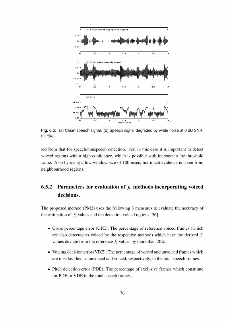
0 0.5 1 1.5 2 2.5 3

−0.5

0

0.5

1 (a) Close speaking speech signal

0 0.5 1 1.5 2 2.5 3

−1

−0.5

0

0.5

1 (b) Degraded speech signal

0 0.5 1 1.5 2 2.5 3

0.8

0.85

0.9

0.95

1 (c) δ(n)

Time (sec) ’

Fig. 6.5: (a) Clean speech signal. (b) Speech signal degraded by white noise at 0 dB SNR.

(c) δ[n].

ied from that for speech/nonspeech detection. For, in this case it is important to detect

voiced regions with a high confidence, which is possible with increase in the threshold

value. Also by using a low window size of 100 msec, not much evidence is taken from

neighbourhood regions.

6.5.2 Parameters for evaluation of f0 methods incorporating voiced

decisions.

The proposed method (PM2) uses the following 3 measures to evaluate the accuracy of

the estimation of f0 values and the detection voiced regions [36].

• Gross percentage error (GPE): The percentage of reference voiced frames (which

are also detected as voiced by the respective method) which have the derived f0

values deviate from the reference f0 values by more than 20%.

• Voicing decision error (VDE): The percentage of voiced and unvoiced frames which

are misclassified as unvoiced and voiced, respectively, in the total speech frames.

• Pitch detection error (PDE): The percentage of exclusive frames which constitute

for PDE or VDE in the total speech frames.

76

The GPE is computed only in the reference voiced frames, which are also detected as

voiced by the f0 methods. If the voicing mechanism in the f0 method detects mostly the

higher SNR voiced regions, then GPE relatively decreases compared to the GPE calcu-

lated with the inclusion the low SNR voiced regions. Better detection of voiced-unvoiced

regions gives a lower VDE and higher GPE, as it includes some low SNR voiced regions

with weak f0 characteristics, which are difficult to estimate. So the PDE indicates better

performance, as it checks for both voiced decisions and f0 estimation.

6.5.3 Description of the fo methods used for comparison.

The evaluation is done for the fo methods with the inbuilt voicing mechanism, i.e., the

autocorrelation (AC), crosscorrelation (CC), RAPT, SHS methods.

• Autocorrelation method (AC): The autocorrelation is applied on the windowed

speech signal frames [91].

• Crosscorrelation method (CC): The crosscorrelation is applied on different speech

signal frames of same size [38].

• Robust algorithm for pitch tracking (RAPT): The method employs normalised cross-

correlation, estimates voiced-unvoiced decisions, and then uses dynamic program-

ming based post processing technique, taking cues from local and contextual infor-

mation [39].

• Subharmonic summation (SHS): The SHS sums the magnitude of several pitch har-

monics of the short-term spectrum to estimate the fundamental frequency. The

routines for the AC, CC and SHS methods were taken from the website in [92] with

the default values for the parameters. The AC, CC and SHS methods have a voic-

ing detection mechanism based on maximum amplitudes derived by the respective

methods. The routine for the RAPT method was downloaded from [93].

6.5.4 Performance of f0 methods.

Performance of the proposed method (PM2) for f0 estimation along with voiced decisions

is given in Tables 6.5 - 6.7 for different degradations.

Table 6.5 shows the performance on the clean, telephone and cellphone speech of the

CSTR database. The best performance with the least PDE score is indicated by a bold

face. The GPE increased for telephone and cellphone speech compared to clean speech.

77

This is because the low frequencies with speech content are attenuated in the telephone

and cellphone speech, increasing both VDE and PDE. Notice that the performance of

proposed method (PM2) is high both in terms of GPE and VDE due to the robustness of

features, thereby giving a least PDE.

Table 6.5: Evaluation results of fo methods for clean speech, telephone and cellphone

speech for different methods. The scores are given in terms of percentage errors of GPE,

VDE and PDE.

Cellphone Telephone Clean

METHOD GPE VDE PDE GPE VDE PDE GPE VDE PDE

PM2 1.86 9.54 10.05 1.61 7.96 8.43 1.48 7.36 7.11

AC 2.62 12.82 13.52 2.50 11.31 12.07 2.09 11.13 11.78

CC 4.17 12.43 13.63 4.24 11.39 12.73 4.09 11.67 12.98

RAPT 14.85 11.34 15.89 10.50 9.12 12.66 6.85 8.16 10.55

SHS 5.83 24.06 25.39 5.29 24.51 25.87 3.49 23.52 24.47

Table 6.6 Evaluation results of fo methods for CSTR database for different types of noises at

three SNR levels by different methods. The scores are given in terms of percentage errors of

GPE, VDE and PDE.

0 dB 10 dB 20 dB

NOISE METHOD GPE VDE PDE GPE VDE PDE GPE VDE PDE

PM2 6.85 16.75 18.17 1.13 8.73 9.38 1.45 8.63 9.02

AC 10.71 31.03 32.51 0.02 21.18 21.19 0.02 22.17 22.26

white CC 8.57 28.57 30.05 0.01 21.18 21.18 14.61 5.06 10.21

RAPT 15.62 20.62 23.24 2.90 9.05 10.05 1.28 5.53 6.03

SHS 47.22 27.59 35.96 13.04 26.60 29.56 19.15 28.57 33.00

PM2 10.61 24.42 25.83 2.73 13.31 14.44 1.21 9.50 9.94

AC 18.75 39.90 42.86 3.03 22.66 22.69 1.75 21.67 22.17

babble CC 14.71 39.41 41.82 5.80 23.15 25.12 3.61 20.22 20.36

RAPT 43.14 37.19 48.24 12.99 32.66 37.69 5.19 14.57 16.58

SHS 52.00 40.89 47.29 25.58 35.96 41.38 17.39 31.03 34.98

PM2 2.89 11.40 12.08 1.49 8.87 9.33 1.56 8.92 9.32

AC 17.78 30.05 33.99 7.75 28.08 28.98 7.54 23.15 23.45

volvo CC 21.74 33.50 38.42 6.56 26.11 28.08 6.28 21.18 21.18

RAPT 12.00 21.61 24.62 2.67 7.54 8.54 1.28 6.53 7.04

SHS 50.00 39.41 47.78 22.45 35.96 41.38 20.83 35.96 40.89

Performance of the fo methods for white, babble and volvo noises at three different

SNRs of 0 dB, 10 dB and 20 dB is shown in Table 6.6. The PDE score is least for

78

the proposed method (PM2) at low SNRs for white noise. The AC and CC methods

have a lesser GPE at 10 dB SNR, however with a higher PDE. It is noticed that only the

high SNR voiced regions are detected as voiced (indicated by higher VDE), which gave

a better GPE. SHS method also performed less, as it was not able to estimate reliable

harmonics. RAPT method performed slightly better than the proposed method (PM2) at

SNR ≥ 20 dB. The proposed method performed well in the cases of babble and volvo

noises due to the robustness of the features used. Notice that the performance of other

standard methods deteriorated, particularly at the low SNRs.

Table 6.7: Evaluation results of fo methods for distance speech by different methods. The scores are given in

terms of percentage errors of GPE, VDE and PDE.

C3 (2 - 3m) C2 (1 - 2m) C1 C0

CASE METHOD GPE VDE PDE GPE VDE PDE GPE VDE PDE GPE VDE PDE

PM2 13.22 17.72 20.68 6.16 17.31 19.23 11.88 13.78 17.60 3.16 6.66 7.93

Car

AC 13.23 21.59 24.46 6.79 16.88 18.41 34.87 16.69 24.60 3.20 6.51 7.55

CC 15.23 21.38 24.98 6.76 15.08 16.75 31.41 16.29 23.69 3.46 6.02 7.20

RAPT 33.41 39.84 48.59 19.49 20.82 25.26 25.90 26.44 31.44 6.39 18.66 20.86

SHS 23.82 35.54 40.13 17.70 30.87 33.48 17.12 34.27 37.94 5.73 25.89 27.69

PM2 14.72 21.05 27.08 8.05 10.63 13.52 7.46 12.11 14.76 2.01 7.04 7.70

Office

AC 15.80 23.76 27.64 3.86 12.73 14.03 2.47 12.84 13.61 3.16 5.42 6.49

CC 16.92 24.05 28.32 4.75 13.07 14.71 3.13 12.80 13.79 3.86 4.32 5.69

RAPT 23.43 23.85 29.31 11.00 20.78 24.42 7.26 18.92 21.38 5.79 9.55 11.61

SHS 19.67 34.84 39.54 6.07 29.44 31.26 4.10 26.91 28.07 4.78 20.23 21.80

PM2 14.02 20.23 23.54 8.61 13.71 16.43 7.18 8.40 10.73 1.88 7.35 7.98

Public

AC 16.30 22.96 26.94 8.78 14.43 17.15 2.59 14.26 15.04 2.14 5.76 6.49

CC 15.74 23.28 27.27 9.23 14.39 17.35 3.19 13.99 14.97 2.28 5.13 5.95

RAPT 29.23 24.69 31.25 18.72 24.91 30.50 9.00 22.99 25.99 5.41 13.41 15.34

SHS 18.53 32.44 37.14 9.75 29.13 31.87 4.55 27.24 28.50 4.84 21.11 22.70

The performance of the fo methods at different distances is shown in Table 6.7. Since

distance speech is time varying there is confusion between voiced and unvoiced regions

even for the high SNR cases of C0 and C1 (see VDE score). The CC method has a slightly

better performance at close speaking (C0) case, but deteriorated at longer distances (C3 -

C1). This is mainly because of proper threshold setting for the detection of voiced regions,

which gave better performance for high SNR close speaking case of C0, but was unable to

perform well for high distance cases (C3 - C1). The proposed method (PM2) performed

relatively better compared to most methods in C3 - C1 cases.

79

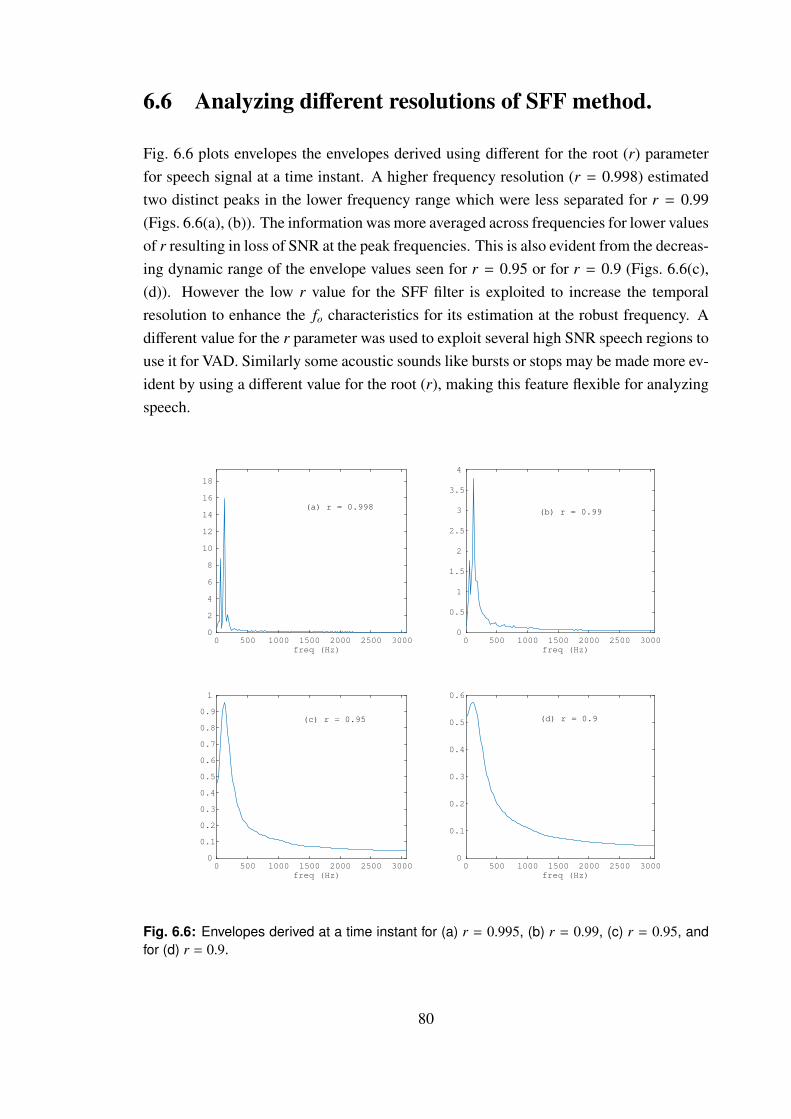
6.6 Analyzing different resolutions of SFF method.

Fig. 6.6 plots envelopes the envelopes derived using different for the root (r) parameter

for speech signal at a time instant. A higher frequency resolution (r = 0.998) estimated

two distinct peaks in the lower frequency range which were less separated for r = 0.99

(Figs. 6.6(a), (b)). The information was more averaged across frequencies for lower values

of r resulting in loss of SNR at the peak frequencies. This is also evident from the decreas-

ing dynamic range of the envelope values seen for r = 0.95 or for r = 0.9 (Figs. 6.6(c),

(d)). However the low r value for the SFF filter is exploited to increase the temporal

resolution to enhance the fo characteristics for its estimation at the robust frequency. A

different value for the r parameter was used to exploit several high SNR speech regions to

use it for VAD. Similarly some acoustic sounds like bursts or stops may be made more ev-

ident by using a different value for the root (r), making this feature flexible for analyzing

speech.

0 500 1000 1500 2000 2500 3000

freq (Hz)

0

2

4

6

8

10

12

14

16

18

(a) r = 0.998

0 500 1000 1500 2000 2500 3000

freq (Hz)

0

0.5

1

1.5

2

2.5

3

3.5

4

(b) r = 0.99

0 500 1000 1500 2000 2500 3000

freq (Hz)

0

0.1

0.2

0.3

0.4

0.5

0.6

0.7

0.8

0.9

1

(c) r = 0.95

0 500 1000 1500 2000 2500 3000

freq (Hz)

0

0.1

0.2

0.3

0.4

0.5

0.6

(d) r = 0.9

Fig. 6.6: Envelopes derived at a time instant for (a) r = 0.995, (b) r = 0.99, (c) r = 0.95, and

for (d) r = 0.9.

80

6.7 Summary

Single frequency filtering (SFF) output contains segments of high signal-to-noise ratio

(SNR), which are exploited for extraction of the fundamental frequency from degraded

speech. The bandwidth of the single frequency filter can be controlled to obtain good

temporal resolution of the envelope of the signal at a given frequency. Higher temporal

resolution helps to preserve the periodicity information in the SFF envelope for the voiced

segment. The periodicity information is derived using the autocorrelation function of the

high SNR segment. The proposed SFF method showed improvement in comparison with

other methods for different types of degradations in speech, including the distant speech.

The method does not involve estimation of noise characteristics, nor it requires any train-

ing data. The proposed method did not rely on degraded f0 harmonics, but used the

temporal characteristics at the robust frequency for f0 estimation. So it performed better

even when the performance of other harmonic-based methods like SWIPE' deteriorated

due to the degraded f0 harmonics.

Note that the single frequency envelopes derived using either DFT (Discrete Fourier

Transform) or by gammatone filters, do not possess the high SNR property of the SFF

method due to averaging effect over the time and frequency band around the selected fre-

quency, respectively. In fact extraction of the fundamental frequency using the envelopes

at each frequency derived using DFT and gammatone filters gave gross error (GE) of 89%

and 46%, respectively, for a clean speech utterance, whereas the proposed SFF-based

method gave a GE of 4.32% for the same data.

In this chapter, a method is proposed for detection of voiced regions along with f0

estimation. The standard methods combining voicing and f0 estimation performed less

in degraded situations. The δ[n] feature with proper thresholding used for detection of

voiced regions, along with the estimation of f0 using the single robust frequency boosted

the performance in degraded conditions for the proposed method.

It may be possible to improve the performance of the f0 extraction further using suit-

able post processing techniques. Also, it may be possible to refine the method by exploit-

ing the high frequency resolution that the SFF method gives when the filtering is done

using a pole very close to the unit circle in the z-plane, i.e., using r = 0.99 [94].

81

Chapter 7

Detection of glottal closure instants

from degraded speech

Glottal closure instant (GCI) is an instant of significant excitation which takes place dur-

ing glottal vibration. Features extracted around the epoch regions are robust to degrada-

tions and would improve the performance of speech systems. Precise estimation of glottal

closure instants (GCIs) is hard in the case of degraded environments as the temporal char-

acteristics are affected by the degradations. Most methods employ features derived using

block processing methods to estimate the information of the GCIs. In this chapter, the

instant characteristics of the GCIs are exploited using the single frequency filtering (SFF)

method.

The impulse-like excitation at the epochs are determined by the sharp discontinuities

in the normalized spectral variance values. The sharpness of spectral variance values is

measured using the slope parameter. The presence of degradations introduced spurious

peaks making it difficult to estimate the GCI. The envelopes are compensated for noise to

reduce this effect. It is observed that with noise compensation, the presence of spurious

peaks in the slope values have reduced. The proposed method is evaluated for different

noises, and is able to give locations of GCIs even at low SNR. The instantaneous features

derived by using SFF method along with noise compensation, are able to exploit the

characteristics of the GCI to give a reliable estimation of the GCIs in the presence of

degradations. Section 7.1 gives the development of the proposed method for the detection

of GCIs. Section 7.2 gives details about the methods used for evaluation along with the

details of speech and noise databases, and evaluation parameters. Performance of different

GCI estimation methods for different noises are discussed in section 7.3. Section 7.4 gives

a summary of this study.

82

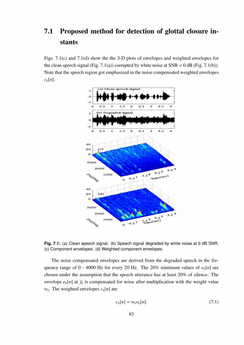
7.1 Proposed method for detection of glottal closure in-

stants

Figs. 7.1(c) and 7.1(d) show the the 3-D plots of envelopes and weighted envelopes for

the clean speech signal (Fig. 7.1(a)) corrupted by white noise at SNR = 0 dB (Fig. 7.1(b)).

Note that the speech region got emphasized in the noise compensated weighted envelopes

ck[n].

Fig. 7.1: (a) Clean speech signal. (b) Speech signal degraded by white noise at 0 dB SNR.

(c) Component envelopes. (d) Weighted component envelopes.

The noise compensated envelopes are derived from the degraded speech in the fre-

quency range of 0 - 4000 Hz for every 20 Hz. The 20% minimum values of ek[n] are

chosen under the assumption that the speech utterance has at least 20% of silence. The

envelope ek[n] at fk is compensated for noise after multiplication with the weight value

wk. The weighted envelopes ck[n] are

ck[n] = wkek[n]. (7.1)

83

The noise compensated envelopes ck[n] are normalized across frequency. The normalized

envelopes ek[n] are given by

ek[n] =ck[n]∑K

l=1 cl[n]. (7.2)

The variance (σ2[n]) is computed from the normalized envelopes. The variance contour

shows discontinuities around the GCIs. The slope of the variance contour is least at GCI

within a glottal cycle. Thus the GCIs are detected by the instant of the lowest slope value

of the variance contour in each glottal cycle. The slope value of the variance contour

at each time instant is obtained from the neighbouring values at each instant. An ap-

proximate estimate of each GCI period is obtained using the zero frequency filter (ZFF)

method [68]. If the minimum of the slope is within 2 msec of the initial estimated GCI,

then the GCI is estimated as the location of the minimum slope, otherwise the initial es-

timate of the GCI is considered as the GCI. It is observed that envelopes obtained by the

SFF method give a better estimation of the GCI compared to the ZFF method in all cases.

Figs. 7.2(c) and 7.2(d) shows the variance (σ2[n]) and slope values, respectively, com-

puted for the envelopes ek[n] derived from the clean speech signal (shown in Fig. 7.2(b)).

The differenced EGG (DEGG) signal indicating the true GCIs is plotted in Fig. 7.2(a) as

reference (ground truth). Notice that the variance (σ2[n]) shows discontinuities/dips in re-

gions around the GCIs (refer Fig. 7.2(c)). The values of the slopes have minimum values

at the locations of the glottal closure instants (Fig. 7.2(d)). Fig. 7.2(e) shows the speech

degraded with white noise at 0 dB SNR. The corresponding clean speech is shown in

Fig. 7.2(b). Figs. 7.2(f)-7.2(i) show the variance (σ2[n]) and slope contours derived from

the envelopes (ek[n]) and the noise compensated envelopes (ck[n]) of the degraded speech.

Notice that the values of σ2[n] and slope derived from the compensated envelopes (ck[n])

show better evidence of the GCIs for the degraded speech signal (Figs. 2(h), 2(i)), when

compared to the values derived from the envelopes (ek[n]) without noise compensation

(refer Figs. 7.2(f), 7.2(g)).

84

0 0.01 0.02 0.03 0.04 0.05 0.06-0.2

-0.1

0

0.1(a) DEGG signal

0 .01 .02 .03 .04 .05 .06-0.5

0

0.5(b) Clean speech signal

0.01 0.02 0.03 0.04 0.05 0.060.5

1

1.510-5

(c) 2[n] derived from envelopes of clean speech

0 0.01 0.02 0.03 0.04 0.05 0.06-1

0

110-6

(d) Slope derived from envelopes of clean speech

0 0.01 0.02 0.03 0.04 0.05 0.06-1

0

1(e) Degraded speech signal

0 0.01 0.02 0.03 0.04 0.05 0.062

4

10-6

(f) 2[n] derived from envelopes of degraded speech

0 0.01 0.02 0.03 0.04 0.05 0.06-2

0

210-7

0 0.01 0.02 0.03 0.04 0.05 0.060

0.5

110-5

(h) 2[n] derived from weighted envelopes of degraded speech

0 0.01 0.02 0.03 0.04 0.05 0.06Time (sec)

-2

0

210-6

(i)) Slope derived from weighted envelopes of degraded speech

Fig. 7.2: (a) DEGG signal. (b) Clean speech signal. (c, d) Variance (σ2[n]) and slope com-

puted from envelopes derived from clean speech. (e) Speech signal degraded by white noise

at 0 dB SNR. (f, g) Variance and slope computed from envelopes of degraded speech. (h, i)

Variance and slope computed from the compensated envelopes of degraded speech.

85

0 .01 .02 .03 .04 .05 .06−0.2

0

0.2(a) DEGG signal

0 0.01 0.02 0.03 0.04 0.05 0.06−5

0

5x 10

−6

(b) Slope (white)

01 0.01 0.02 0.03 0.04 0.05 0.06−2

0

2x 10

−6

(c) Slope (babble)

0 0.01 0.02 0.03 0.04 0.05 0.06−1

0

1x 10

−6

(d) Slope (machinegun)

0 0.01 0.02 0.03 0.04 0.05 0.06−2

0

2x 10

−6

(e) Slope (f16)

0 0.01 0.02 0.03 0.04 0.05 0.06−2

0

2x 10

−6

Time (sec)

(f) Slope (hfchannel)

Fig. 7.3: (a) DEGG signal. Values of slope derived from compensated envelopes for the

speech degraded at 10 dB SNR with (b) white noise, (c) babble noise, (d) machine gun noise

(e) f16 noise, (h) hfchannel noise.

Fig. 7.3 shows the plots of the slope values derived from the compensated envelopes

(ck[n]) for speech degraded with five different degradations at 10 dB SNR, along with

the DEGG signal. The characteristics of the noise affect the GCI estimation in different

ways for each noise, as seen from the slope contours (Figs. 7.3(b)- 7.3(f)). However the

slope values derived from the noise compensated envelopes still give good evidence of

the locations of GCIs in most cases.

86

7.2 Evaluation of the different GCI methods across dif-

ferent degradations

7.2.1 Database

The methods are evaluated on speech signals from CMU ARCTIC database [95], cor-

rupted by noises from NOISEX database [75]. Three hundred random utterances are

taken from phonetically balanced English sentences, spoken by three speakers: BDL (US

male), JMK (US male) and SLT (US female). The duration of each utterance is approx-

imately 3 sec. Noises are added at SNRs of 0 dB and 10 dB. All the speech signals are

downsampled to 8 kHz.

7.2.2 Methods used for detection of GCIs.

The following methods are used for comparison:

• MSM method: The subset of samples with lowest singularity exponent values are

used to detect the GCIs. It relies on the precise estimation of multiscale parameter

(singularity exponent) at each instant in the signal domain [66].

• YAGA method: The information for the voice source signal obtained from the it-

erative adaptive inverse filtering (IAIF) is further analysed using stationary wavelet

transform across different wavelet scales. The discontinuities are detected using

group delay function, and the GCI candidates are measured as negative going zero

crossings. The falsely detected GCIs are then removed using the M-best dynamic

programming approach [96].

• DYPSA method: The method uses zero-crossings of the phase-slope function, en-

ergy weighted group-delay, and a phase-slope projection technique to recover some

of the candidates [97].

• ZFF method: The zero-frequency filter consists of an ideal resonator with four real

poles on the unit circle in the z-plane, followed by a trend removal operation. The

positive zero crossings in the resulting ZFF output represent the instants of glottal

closure. The effects of vocal tract resonances and noise are suppressed, as they are

significant mainly in the frequencies much above 0 Hz [68].

87

7.2.3 Parameters for evaluation of GCI detection methods

The following parameters are used for evaluation of GCI detection methods as mentioned

in [97].

• Identification rate (IDR) : The percentage of glottal cycles for which exactly one

epoch is detected.

• Miss rate (MR): The percentage of glottal cycles for which no epoch is detected.

• False alarm rate (FAR): The percentage of glottal cycles for which more than one

epoch is detected.

• Identification rate2 (IDR2): Identification rate within the range of -0.25 to 0.25

msec.

For better performance, IDR and IDR2 values should be high with low MR and

FAR. IDR2 measure indicates that the correctly identified epochs should be in closer

range with reference epochs.

7.3 Performance of the proposed method for GCI detec-

tion

The proposed method has been evaluated without and with noise compensation, indicated

by PM (UW), PM (W), respectively. Table 7.1 shows the results obtained by the proposed

and other methods across different noises at the SNRs of 0 dB and 10 dB. Notice that the

noise compensation has significantly increased the IDR2 value. The presence of spurious

noise peaks in the degraded conditions makes it difficult for precise estimation of the

glottal closure instants. The noise compensation technique used in the proposed method

reduces the spurious noise peaks. There is good improvement in the IDR2 score for

PM(W) method in the low SNR nonstationary noises due to noise compensation. The

noise compensation technique gives good performance for different stationary and time

varying noises. Notice that the improvement is significant in both high and low SNR

cases, as the speech characteristics are evident after compensating for noise. The method

with better IDR1 score might have considered the regions with weak GCI characteristics,

but was unable to a give a precise estimation. On the other hand a different method might

88

Table 7.1: Evaluation results of GCI methods for different types of noises at SNRs of 0 dB

and 10 dB.

NOISE (SNR) METHOD IDR MR FAR IDR2

PM (UW) 96.46 2.24 1.29 19.62

PM (W) 96.35 2.32 1.33 30.81

white (0) MSM 78.17 3.38 18.45 34.72

YAGA 78.61 0.60 20.78 30.34

DYPSA 68.30 0.83 30.86 37.78

ZFF 95.26 3.84 0.90 8.19

PM (UW) 98.35 0.99 0.66 18.69

PM (W) 98.33 1.03 0.64 47.25

white (10) MSM 90.33 1.89 7.78 54.23

YAGA 92.30 0.53 7.18 53.16

DYPSA 67.57 0.80 31.63 50.50

ZFF 97.57 2.05 0.38 2.56

PM (UW) 89.99 2.52 7.49 19.16

PM (W) 90.37 2.32 7.31 44.44

babble (0) MSM 81.25 3.31 15.44 35.68

YAGA 77.39 0.87 21.74 41.57

DYPSA 68.30 0.83 30.86 37.78

ZFF 89.63 1.79 8.58 12.55

PM (UW) 97.52 0.95 1.53 34.88

PM (W) 97.71 0.90 1.39 66.27

babble (10) MSM 90.71 1.86 7.43 51.67

YAGA 93.80 0.64 5.56 65.13

DYPSA 87.38 1.22 11.40 60.19

ZFF 96.93 1.79 1.28 3.20

PM (UW) 92.16 5.21 2.63 51.29

PM (W) 90.37 2.32 7.31 44.44

machine gun (0) MSM 81.25 3.31 15.44 35.68

YAGA 77.39 0.87 21.74 41.57

DYPSA 93.74 1.55 4.71 71.37

ZFF 93.21 5.89 0.90 6.40

PM (UW) 96.06 2.41 1.53 57.19

PM (W) 96.28 2.36 1.36 78.00

machine gun (10) MSM 93.41 2.49 4.11 55.86

YAGA 96.12 0.93 2.95 86.33

DYPSA 95.21 1.39 3.40 75.80

ZFF 96.41 2.94 0.64 4.10

PM (UW) 73.52 8.96 17.52 14.64

PM (W) 74.11 8.78 17.11 36.59

f16 (0) MSM 80.60 3.52 15.88 35.65

YAGA 67.38 1.96 30.66 36.40

DYPSA 55.37 0.93 43.69 33.47

ZFF 81.05 2.18 16.77 9.09

PM (UW) 96.91 2.11 0.98 28.14

PM (W) 97.19 2.01 0.80 60.94

f16 (10) MSM 90.91 1.97 7.13 53.05

YAGA 92.44 0.71 6.86 61.23

DYPSA 81.66 1.11 17.23 56.59

ZFF 96.16 3.33 0.51 6.91

89

NOISE (SNR) METHOD IDR MR FAR IDR2

PM (UW) 98.34 0.84 0.82 24.63

PM (W) 98.33 0.85 0.81 37.00

hfchannel (0) MSM 77.19 3.68 19.13 32.08

YAGA 84.39 0.54 15.07 28.23

DYPSA 42.88 0.49 56.62 23.70

ZFF 96.54 2.82 0.64 3.97

PM (UW) 98.61 0.77 0.61 22.65

PM (W) 98.75 0.72 0.53 52.54

hfchannel (10) MSM 89.67 2.02 8.32 51.82

YAGA 92.64 0.56 6.80 49.92

DYPSA 71.60 0.98 27.42 44.76

ZFF 97.44 1.79 0.77 2.18

PM (UW) 83.44 14.55 2.01 11.66

PM (W) 83.74 14.48 1.78 25.21

buccaneer1 (0) MSM 79.77 3.18 17.05 34.37

YAGA 78.46 1.57 19.97 31.14

DYPSA 45.60 0.61 53.79 28.10

ZFF 81.95 16.77 1.28 8.96

PM (UW) 96.70 2.27 1.03 20.17

PM (W) 96.80 2.21 0.98 52.77

buccaneer1 (10) MSM 90.56 1.93 7.51 52.28

YAGA 93.24 0.71 6.05 54.50

DYPSA 75.47 1.10 23.42 51.33

ZFF 96.03 3.46 0.51 9.48

PM (UW) 88.31 9.63 2.06 14.38

PM (W) 88.58 9.53 1.89 28.25

buccaneer2 (0) MSM 80.60 3.36 16.04 38.92

YAGA 63.40 1.29 35.32 38.17

DYPSA 42.41 0.63 56.96 32.20

ZFF 85.15 14.08 0.77 10.76

PM (UW) 97.85 1.39 0.77 22.63

PM (W) 97.89 1.33 0.78 54.45

buccaneer2 (10) MSM 90.79 2.06 7.16 55.36

YAGA 91.89 0.60 7.51 60.38

DYPSA 72.85 0.87 26.28 55.40

ZFF 96.54 2.82 0.64 3.97

have detected only high SNR voiced regions and hence was able to give GCI locations

precisely. So the comparison of IDR2 score is possible only when the methods have

similar IDR1 score. The ZFF method was unable to give precise location of the GCIs,

and was able to estimate only 2.56 % percent of the regions precisely, when the proposed

method was able to estimate 47.26 % regions correctly (for speech degraded by white

noise at 10 dB SNR). The proposed, MSM, YAGA, DYPSA and ZFF methods are all

affected by degradation. However, the improvement of the proposed method over YAGA,

MSM, DYPSA and ZFF methods is due to noise compensation (Table 7.1). Notice that

the instants of discontinuities related to glottal closure are more prominent when derived

at a sample level, and hence the justification for using SFF method.

90

7.4 Summary

Methods for detection of glottal closure instants in degraded conditions have been pro-

posed in this chapter. The impulse-like discontinuities of the glottal closure instants is

felt at all frequencies, which is exploited using the slope of the variance computed from

the envelopes derived using the single frequency filtering method. Performance of the

proposed method improved significantly the precision for GCI detection with the incor-

poration of the noise compensation.

91

Chapter 8

Enhancement of degraded speech

The presence of noise in speech reduces the quality and intelligibility of speech. Degrada-

tion of speech also affects the ability of a person to understand what the speaker is trying

to communicate. In reality we can not accurately estimate the characteristics of the noise

and the clean speech signal, from the degraded speech signal. Note that when speech

and noise are intermixed, they often get confused. A high suppression of noise deterio-

rates the speech characteristics, whereas a low suppression would not remove the effect

of noise. It is required to have a method to enhance the degraded speech across different

environments, without having to learn the characteristics of degradation for each case. In

this chapter, a method is proposed to improve the comfort level of the listener by reduc-

ing the effect of the noise. It has been observed that speech features are reflected better

after compensating for the noise at each frequency. The features thus derived from the

compensated envelopes are further exploited by deriving weight functions to see whether

it enhances the degraded speech for better comfort level of listening.

In this chapter different weight functions are derived by computing features at differ-

ent resolutions using the single frequency filtering (SFF) method. The root of the filter in

the single frequency filtering (SFF) method is modified to achieve better temporal resolu-

tion required to enhance speech at the fine level. Temporal gross and fine weight functions

derived from the noise compensated envelopes are applied to the degraded speech to get

enhanced speech. The enhanced speech seems to have a better comfort level for listening.

The method does not require the need of training data, and does not have any threshold

estimation for noise suppression. The method is evaluated for different types of degrada-

tions.

Sections 8.1 gives the development of the method proposed for speech enhancement

using gross and fine weight functions. Section 8.2 gives details about the database, eval-

uation criteria along with the results. Section 8.3 gives the summary of the study.

92

8.1 Proposed method for enhancement of degraded speech.

8.1.1 Estimation of the gross weight function g[n].

The characteristics of speech signal can not be estimated properly from the features de-

rived from the degraded speech. Hence it is appropriate to suppress the noise charac-

teristics in a manner not diminishing the speech characteristics. The noise compensation

technique proposed in chapter 4 rightly enhances speech and deemphasizes the noise char-

acteristics. The amplitude envelopes ek[n] are computed in the frequency range of 300 -

4000 Hz. The r value of the single-pole filter is chosen as 0.99 to achieve high frequency

resolution. The noise compensation technique uses the minimal 20% of ek[n] values at

the desired frequency fk to derive the normalized weight value (wk) given by

wk =

1µk∑N

l=11µl

, (8.1)

where N is the number of channels. The ek[n] values are weighted with wk to derive

weighted ck[n] values. It is observed that the noise floor at each frequency has signifi-

cantly decreased for the weighted envelopes compared to the unweighted envelopes. Thus

the features derived from the weighted envelopes are robust to degradations. Speech re-

gions stand out better after noise compensation, and are further processed to enhance

speech.

The mean (µ[n]) or standard deviation (σ[n]) of the square of the weighted envelopes

are further exploited to give the gross weight function g[n]. The values of (σ[n] − µ[n])

have been observed to be high for speech regions which is further enhanced with the high

amplitudes of (σ[n] + µ[n]) value to give (σ2[n] − µ2[n]) value. The dynamic range of

(σ2[n] − µ2[n]) has been reduced by taking a root of order 128th on the absolute value of

(σ2[n] − µ2[n]) giving the value [n]. The root value is more for [n] in order to decrease

the dynamic range. The [n] values are smoothed over 200 msec window to give g[n].

Fig. 8.1 shows the clean speech, speech degraded by white noise at 0 dB SNR and the

gross weight function g[n] derived from the degraded speech. Notice that the g[n] values

for noise/nonspeech regions are low. So weighting (multiplying) degraded speech with

the corresponding g[n] values would decrease the effect of noise. The speech regions

exhibit high g[n] values and are enhanced.

93

0 1 2 3 4 5 6 7 8−1

−0.5

0

0.5

1

(a) Clean speech signal

0 1 2 3 4 5 6 7 8−1

−0.5

0

0.5

1

(b) Degraded speech signal

0 1 2 3 4 5 6 7 8

0

0.02

0.04

Time(sec)

(c) Gross weight function (g[n])

Fig. 8.1: (a) Clean speech signal. (b) Speech degraded by white noise at 0 dB SNR. (c) Gross

weight function (g[n]).

8.1.2 Estimation of the fine weight function f [n].

The [n] values are also derived by adjusting the bandwidth of the SFF method for achiev-

ing good temporal resolution. The root (r value) of the single pole H(z) filter is modified

to 0.95 to have high temporal resolution. The envelopes thus derived are then compen-

sated for the effect of noise. The [n] values derived at every sample n for r = 0.95 is

denoted by f [n], and would correspond to the amplitude changes at the fine level. Fig. 8.2

shows the clean speech, speech degraded by white noise and the fine weight function f [n].

Notice that the changes/fluctuations at the sample level are observed better in f [n] values

compared to the degraded speech (Figs. 8.2(b), 8.2(c)). Also the fluctuations are evident

only when the envelopes are computed at high temporal resolution with r = 0.95. The de-

graded speech signal weighted using the gross weight function (g[n]) is further weighted

with the fine weight function ( f [n]) to give the enhanced speech signal.

Figs. 8.3 and 8.4 show the degraded speech, enhanced speech and their correspond-

ing spectrograms for speech signals degraded by white and babble noises at SNR of

5 dB. The reduction of noise effect is seen from both the enhanced speech waveforms

(Figs. 8.3(b), 8.4(b)) and their spectrograms (Figs. 8.3(d), 8.4(d)).

94

0 0.05 0.1 0.15 0.2 0.25 0.3−1

−0.5

0

0.5

1(a) Clean speech signal

0 0.05 0.1 0.15 0.2 0.25 0.3−1

−0.5

0

0.5

1(b) Degraded speech signal

0 0.05 0.1 0.15 0.2 0.25 0.3

0.35

0.4

0.45

0.5

Time(sec)

(c) Fine weight function (f[n])

Fig. 8.2: (a) Clean speech signal. (b) Degraded speech signal. (c) Fine weight function ( f [n]).

0 0.5 1 1.5 2 2.5 3 3.5 4-1

0

1(a) Degraded speech signal

0 0.5 1 1.5 2 2.5 3 3.5 4-1

0

1 (b) Enhanced speech signal

(c) Spectrogram of (a)

0 0.5 1 1.5 2 2.5 3 3.5 4Time (sec)

0

1

2

3

Fre

qu

en

cy (

kH

z)

(d) Spectrogram of (b)

0 0.5 1 1.5 2 2.5 3 3.5 4Time (sec)

0

1

2

3

Fre

qu

en

cy (

kH

z)

Fig. 8.3: (a) Speech degraded by white noise at 5 dB SNR. (b) Enhanced speech signal. (c)

Spectrogram of the degraded speech signal. (d) Spectrogram of the enhanced speech signal.

8.2 Discussion.

A subset of 10 utterances are considered from the TIMIT TEST database for five male

and five female speakers [76], along with a few utterances of distance speech (C3) [79].

Each utterance is of a different speaker and of a different sentence. Samples of NOI-

SEX database [75] were added to TIMIT TEST database at SNRs of -10 dB and 5 dB.

95

0 0.5 1 1.5 2 2.5 3 3.5-1

0

1(a) Degraded speech signal

0 0.5 1 1.5 2 2.5 3 3.5-1

0

1(b) Enhanced speech signal

(c) Spectrogram of (a)

0 0.5 1 1.5 2 2.5 3 3.5Time (sec)

0

1

2

3

Fre

qu

en

cy (

kH

z)

(d) Spectrogram of (b)

0 0.5 1 1.5 2 2.5 3 3.5Time (sec)

0

1

2

3

Fre

qu

en

cy (

kH

z)

Fig. 8.4: (a) Speech degraded by babble noise at 5 dB SNR. (b) Enhanced speech signal. (c)

Spectrogram of the degraded speech signal. (d) Spectrogram of the enhanced speech signal.

Seven people were asked to rate whether the enhanced speech is of better intelligibility

and quality. The performance of the speech enhancement method is measured in terms

of quality and intelligibility of the enhanced speech in comparison with degraded speech.

The quality of the degraded speech signal does not necessarily indicate intelligibility of

the speech signal. Listeners felt that the utterances after weighting had significant reduc-

tion in the background noise, giving a better quality speech. The reduction in background

noise made it easier for listeners to listen and concentrate on the actual speech, due to

which listeners also felt that the enhanced speech was more intelligible. The enhance-

ment method reduced the noise effect irrespective of type of noise.

Most enhancement methods also try to reduce the effect of noise at several frequen-

cies, rather than just weighting the speech signal. The proposed method does not reduce

noise embedded in speech regions, and hence does not perform enough to compare with

the standard enhancement methods. This envisions to deemphasize noise regions using

the proposed weight functions, and then enhance speech to perceive it better.

96

8.3 Summary

Time varying weight functions are derived to enhance the degraded speech, irrespective

of the type of degradation. The root of the single-pole filter used in the single frequency

filtering (SFF) method is modified to derive envelopes at the required resolution. A gross

weight function at a high frequency resolution is derived to reduce the effect of the noise.

Another weight function is derived to enhance the fluctuations at the finer level computing

the envelopes by adjusting the root of the filter for a better temporal resolution. The

method was tested for different degradations, and the enhanced speech was perceived

with better comfort compared to the degraded speech due to reduction of the noise effect.

97

Chapter 9

Summary and Conclusions

The signal-to-noise ratio (SNR) of speech varies along time and frequency. Most speech

processing methods smear information either in the time domain or in the frequency do-

main which leads to loss of information. A signal processing method is derived that

highlights significant events of the speech signal. Speech in real life is prone to vari-

ous degradations, and the features derived are affected by degradations. Human beings

have no issue in understanding and processing speech for different applications due to

redundancy and their knowledge at the semantic levels. However, there is need to de-

velop robust features for speech systems to work across degradations. Methods have

been implemented with trained statistical models for speech systems to work in degraded

environments. However the mismatch in environmental conditions led to deteriorating

performance for speech systems. The main aim of the thesis is to develop features which

are robust to degradations. It is important to aim real world degradations apart from sim-

ulated degradations. Most methods tackle with simulated degradations where the noise

is artificially added to speech signal, which are usually separated by distribution of the

features. It is required to test speech systems in unknown conditions without any prior

data or knowledge.

In this thesis, the single frequency filtering (SFF) method is proposed to highlight the

speech features even from the degraded speech signal. The method overcomes extracts

information at high frequency resolution. The method extracts temporal envelopes at each

frequency, which represents the amplitude information at each time instant. The informa-

tion derived at different frequencies is used to derive robust speech-specific features by

exploiting the varying signal-to-ratio (SNR) characteristic of speech. The method uses a

infinite impulse response (IIR) filter with a pole close to the unit circle, and extracts infor-

mation at the highest carrier frequency (i.e., half the sampling frequency). Since the IIR

filter at a fixed frequency is used to derive amplitude envelopes at different frequencies, it

98

avoids the different gain effects which would arise if different filters were chosen to derive

the amplitude information at different frequencies. Also the SFF method overcomes the

effects of block processing as it uses an IIR filter to derive the spectral information.

Speech is produced by time varying source and vocal tract system. Robust features

corresponding to the manifestation of the source and system characteristics are to be ex-

ploited to tackle speech in degraded situations. The characteristics of speech signal and

noise at each frequency have been exploited for robustness. Speech signal has distinc-

tive behaviour across frequencies due to its more correlative behaviour among its sam-

ples compared to the noise samples. Speech signal has high SNR, particularly at some

frequencies, unlike noise whose power gets distributed more uniformly across frequen-

cies. In this work, a noise compensation technique is proposed which suppresses the

noise component at each frequency. The signal-to-ratio (SNR) of speech computed by

processing speech at individual frequencies is proved to be higher compared to subband

processing of frequencies. This forms the basis of the proposed noise compensation tech-

nique. The estimate of noise at each frequency is computed from the floor created due

to the uncorrelative behaviour of the noise samples. The single frequency filtering (SFF)

method gives amplitude envelopes at the required frequency. The features derived using

SFF method are exploited for voice activity detection (VAD), estimation of fundamental

frequency ( fo), detection of glottal closure instants (GCIs), and for enhancement of de-

graded speech. The proposed methods have been tested for a variety of degradations. Due

to the robustness of the features involved, the proposed methods are able to perform even

for the realistic scenarios like distant speech. The methods have been tested for unknown

situations without any prior knowledge, and the methods also did not use data for training

of statistical models.

Voice activity detection (VAD) is the building block for speech systems, and it is re-

quired to be robust to degradations for reliable performance of speech systems. The pro-

posed method uses the noise-compensated envelopes to derive a robust feature δ[n]. The

δ[n] measure based on the spectral mean and variance of the compensated envelopes is

seen to highlight the speech characteristics in the degraded signal. The proposed method

uses different parameters for the decision logic based on the approximated SNR value

(ρ). An adaptive threshold is derived for each utterance from the minimal δ[n] values.

The nonspeech beginning criteria had played a significant role for the estimation of noise

characteristics, threshold and other parameters in decision logic for the standard methods.

The proposed method does not use any such criteria. Methods have also been developed

for VAD for transient noises and other noises incorporating instantaneous features derived

using the SFF method.

The high SNR of speech at a single robust frequency for a frame is used for fo ex-

99

traction. The root of the filter used in SFF filter is exploited to increase the temporal

resolution to enhance the fo characteristics. The fo estimation was also incorporated with

voicing decisions to give a reliable fo estimate for speech systems.

The method proposed for glottal closure instants (GCI) detection was able to estimate

the location with a high precision. The discontinuity due to the impulse-like excitation of

the GCI is reflected in the spectral variance as sharp fluctuations. The measure of disconti-

nuity is determined by computing the slope of the spectral variance, and the regions where

the slope is minimum is detected as GCIs. The features derived from the envelopes after

compensating for noise are explored to see their effect on enhancement of the degraded

speech. Time varying weight functions are derived at different resolutions by adjusting

the bandwidth of the filter used in the SFF method. The enhanced speech was perceived

to give better comfort level for listening due to reduction of noise effect.

9.1 Major contributions of the work

The major contributions of the research work carried out as a part of this thesis are listed

as follows:

• A new signal processing method called single frequency filtering (SFF) method is

proposed which gives high signal-to-noise ratio (SNR) regions in both time and

frequency domains for speech affected with different types of degradations.

• A new method for speech/nonspeech detection is proposed exploiting the high SNR

features in the SFF outputs of degraded speech. The procedure works for all types

of degradations, without specifically tuning for any specific type of degradation.

• The high SNR characteristic of the SFF output is also exploited for estimating the

fundamental frequency ( fo) by exploiting information at the frequency that gives

the highest SNR for that segment.

• The noise compensation technique proposed for VAD is applied for extracting the

location of the significant impulse-like excitation within a glottal cycle. This is

because the noise compensated envelopes show distinct changes in the slope of the

spectral variance computed as a function of time.

• The noise compensated SFF envelopes derived at different frequency resolutions are

used to derive gross and fine weight functions, as a function of time. The combined

weight functions when applied to the degraded speech signal produces enhanced

100

speech for speech affected by different types of degradations, thus improving the

comfort level of listening.

9.2 Directions for future work

In the thesis the potential of the single frequency filtering (SFF) method for processing

speech is demonstrated for different types of degradations. It is possible that due to the

smearing of temporal features in the SFF output, some of the important features for de-

velopment of speech systems may be lost. Some of the issues that need to be addressed

are listed as follows:

• The proposed method for VAD has been tested for human speech versus degrada-

tions. However in reality, there would be situations where the background noise is

also human, but of a different speaker. Methods should be developed to detect the

speech of the main speaker.

• VAD methods should incorporate features at the source ( fo and tone) and supraseg-

mental level. This features might be combined in a hierarchical fashion, and a

decision logic should be adapted based on several conclusions.

• Features derived from SFF outputs can be used to develop robust speech systems

like speech and speaker recognition.

• The resolutions obtained using the SFF method could be exploited to analyze and

detect acoustic events like voice onset points, voice bars, nasals, etc., and for tasks

like speech segmentation.

• Techniques need to be developed for synthesis of speech after noise compensation,

overcoming the phase effects.

101

List of Publications

Journals

1. G. Aneeja and B. Yegnanarayana, “Exploiting robust frequencies for extraction of

fundamental frequency from degraded speech using temporal envelopes at high SNR

frequencies”, IEEE/ACM Trans. on Audio, Speech, Language Process., vol. 25, no.

4, pp. 829 - 838, April 2017.

2. G. Aneeja and B. Yegnanarayana, “Single frequency filtering approach for discrim-

inating speech and nonspeech”, IEEE/ACM Trans. on Audio, Speech, Language

Process., vol. 23, no. 4, pp. 705 - 717, April 2015.

Conferences

1. P. Vishala, G. Aneeja, Sudersana Reddy Kaidiri and B. Yegnanarayana, ‘Robust

estimation of fundamental frequency using single frequency filtering approach’’, in

Proc. Interspeech 2016, pp. 2155-2158.

2. G. Aneeja, B. Yegnanarayana, “Speech detection in transient noises’’, in Proc. In-

terspeech 2014, Singapore, pp. 2356-2360.

102

References

[1] T. Kinnunen, E. Chernenko, M. Tuononen, P. Franti, and H. Li, “Voice activity

detection using MFCC features and support vector machine,” Proc. Int. Conf. Speech

Comput., vol. 2, pp. 556–561, Oct. 2007.

[2] I. McCowan, D. Dean, M. McLaren, R. Vogt, and S. Sridharan, “The delta-phase

spectrum with application to voice activity detection and speaker recognition,” IEEE

Trans. Audio, Speech, Lang. Process., vol. 19, no. 7, pp. 2026–2038, Sep. 2011.

[3] J. Haigh and J. Mason, “Robust voice activity detection using cepstral features,” in

Proc. IEEE TENCON, 1993, pp. 321–324.

[4] N. Dhananjaya and B. Yegnanarayana, “Voiced/nonvoiced detection based on ro-

bustness of voiced epochs,” IEEE Signal Process. Lett., vol. 17, no. 3, pp. 273–276,

Mar. 2010.

[5] T. Pham, M. Stark, and E. Rank, “Performance analysis of wavelet subband based

voice activity detection in cocktail party environment,” in Proc. Int. Conf. Comput.

and Commun. Technologies, Oct. 2010, pp. 85–88.

[6] Z. Song, T. Zhang, D. Zhang, and T. Song, “Voice activity detection using higher-

order statistics in the teager energy domain,” in Proc. Wireless Commun. Signal

Process., Nov. 2009, pp. 1–5.

[7] Y. W. Jitong Chen and D. Wang, “A feature study for classification-based speech

separation at low signal-to-noise ratios,” IEEE Trans. Audio, Speech, Lang. Process.,

vol. 22, no. 12, pp. 1993–2002, Dec. 2014.

[8] X.-L. Zhang and D. Wang, “Boosted deep neural networks and multi-resolution

cochleagram features for voice activity detection,” in Proc. Interspeech, Sep. 2014,

pp. 1534–1538.

[9] J. Ramrez, J. C. Segura, C. Bentez, A. D. L. Torre, and A. Rubio, “Efficient voice ac-

tivity detection algorithms using long-term speech information,” Speech Commun.,

vol. 42, pp. 3–4, April 2004.

[10] Y. Ma and A. Nishihara, “Efficient voice activity detection algorithm using long-

term spectral flatness measure,” EURASIP Journal on Audio, Speech, Music Pro-

cess., vol. 2015, no. 1, p. 71, 2015.

103

[11] P. Ghosh, A. Tsiartas, and S. Narayanan, “Robust voice activity detection using

long-term signal variability,” IEEE Trans. Audio, Speech, Lang. Process., vol. 19,

no. 3, pp. 600–613, Mar. 2011.

[12] A. Tsiartas, T. Chaspari, N. Katsamanis, P. K. Ghosh, M. Li, M. Van Segbroeck,

A. Potamianos, and S. Narayanan, “Multi-band long-term signal variability features

for robust voice activity detection,” in Proc. Interspeech, Aug. 2013, pp. 718–722.

[13] M. Van Segbroeck, A. Tsiartas, and S. Narayanan, “A robust frontend for VAD:

exploiting contextual, discriminative and spectral cues of human voice,” in Proc.

Interspeech, Aug. 2013, pp. 704–708.

[14] ETSI, Voice activity detector (VAD) for adaptive multirate (AMR) speech traffic

channels, ETSI EN 301 708 v.7.1.1, Dec. 1999.

[15] http://www.3gpp.org/ftp/Specs/html-info/26104.htm.

[16] A. Davis, S. Nordholm, and R. Togneri, “Statistical voice activity detection using

low-variance spectrum estimation and an adaptive threshold,” IEEE Trans. Audio,

Speech, Lang. Process., vol. 14, no. 2, pp. 412–424, Mar. 2006.

[17] J. Sohn, N. S. Kim, and W. Sung, “A statistical model-based voice activity detec-

tion,” IEEE Signal Process. Lett., vol. 6, no. 1, pp. 1–3, 1999.

[18] T. Pham, C. Tang, and M. Stadtschnitzer, “Using artificial neural network for ro-

bust voice activity detection under adverse conditions,” in Proc. Int. Conf. Comput.

Commun. Technol., July 2009, pp. 1–8.

[19] D. Ying, Y. Yan, J. Dang, and F. Soong, “Voice activity detection based on an unsu-

pervised learning framework,” IEEE Trans. Audio, Speech, Lang. Process., vol. 19,

no. 8, pp. 2624 –2633, Nov. 2011.

[20] X.-L. Zhang and J. Wu, “Deep belief networks based voice activity detection,” IEEE

Trans. Audio, Speech, Lang. Process., vol. 21, no. 4, pp. 697–710, April 2013.

[21] J. Ramirez, J. Segura, C. Benitez, A. De la Torre, and A. Rubio, “An effective sub-

band OSF-based VAD with noise reduction for robust speech recognition,” IEEE

Trans. Speech Audio Process., vol. 13, no. 6, pp. 1119–1129, Nov. 2005.

[22] P. Harding and B. Milner, “On the use of machine learning methods for speech and

voicing classification,” in Proc. Interspeech, Sep. 2012.

[23] F. Germain, D. L. Sun, and G. J. Mysore, “Speaker and noise independent voice

activity detection,” in Proc. Interspeech, Aug. 2013, pp. 732–736.

[24] R. Talmon, I. Cohen, and S. Gannot, “Transient noise reduction using nonlocal dif-

fusion filters,” IEEE Trans. Audio, Speech, Lang. Process., vol. 19, no. 6, pp. 1584–

1599, Aug. 2011.

[25] C. Clavel, T. Ehrette, and G. Richard, “Events detection for an audio-based surveil-

lance system,” in Proc. IEEE Int. Conf. Multimedia and Expo (ICME), 2005, pp.

1306–1309.

104

[26] N. Cho and E.-K. Kim, “Enhanced voice activity detection using acoustic event

detection and classification,” IEEE Trans. Consum. Electron., vol. 57, no. 1, pp.

196–202, Feb. 2011.

[27] I. Volfin and I. Cohen, “Dominant speaker identification for multipoint videoconfer-

encing,” Computer Speech & Language, vol. 27, no. 4, pp. 895–910, July 2013.

[28] S. Mousazadeh and I. Cohen, “Voice activity detection in presence of transient noise

using spectral clustering,” IEEE Trans. Audio, Speech, Lang. Process., vol. 21, no. 6,

pp. 1261–1271, June 2013.

[29] R. Cai, L. Lu, H.-J. Zhang, and L.-H. Cai, “Highlight sound effects detection in

audio stream,” in Proc. Int. Conf. Multimedia and Expo, vol. 3, July 2003, pp. 37–

40.

[30] K. N. Ross and M. Ostendorf, “A dynamical system model for generating funda-

mental frequency for speech synthesis,” IEEE Trans. Audio, Speech, Lang. Process.,

vol. 7, no. 3, pp. 295–309, May 1999.

[31] D. R. Feinberg, B. C. Jones, A. C. Little, D. M. Burt and D. I. Perrett, “Manipulations

of fundamental and formant frequencies influence the attractiveness of human male

voices,” Animal Behaviour, vol. 69, no. 3, pp. 561–568, Mar. 2005.

[32] P. F. Assmann, S. Dembling, and T. M. Nearey, “Effects of frequency shifts on per-

ceived naturalness and gender information in speech,” in Proc. Interspeech, Mar.

2006, pp. 889–892.

[33] L. Geurts and J. Wouters, “Coding of the fundamental frequency in continuous inter-

leaved sampling processors for cochlear implants,” J. Acoust. Soc. Amer., vol. 109,

no. 2, pp. 713–726, Feb. 2001.

[34] M. Sambur, “Selection of acoustic features for speaker identification,” IEEE Trans.

Acoust., Speech and Signal Process., vol. 23, no. 2, pp. 176–182, Sep. 1975.

[35] A. Ljolje, “Speech recognition using fundamental frequency and voicing in acoustic

modeling,” in Proc. Int. Conf. Spoken Lang. Process., 2002, pp. 2177–2140.

[36] W. Chu and A. Alwan, “Reducing F0 frame error of F0 tracking algorithms under

noisy conditions with an unvoiced/voiced classification frontend,” in Proc. IEEE Int.

Conf. Acoust., Speech, Signal Process., April 2009, pp. 3969–3972.

[37] L. Rabiner, “On the use of autocorrelation analysis for pitch detection,” IEEE Trans.

Acoust., Speech, Signal Process., vol. 25, no. 1, pp. 24–33, Feb. 1977.

[38] S. A. Samad, A. Hussain, and L. K. Fah, “Pitch detection of speech signals using the

cross-correlation technique,” in Proc. IEEE TENCON, vol. 1, 2000, pp. 283–286.

[39] D. Talkin, “A robust algorithm for pitch tracking (RAPT),” Speech coding and syn-

thesis, vol. 495, p. 518, 1995.

105

[40] A. D. Cheveigne and H. Kawahara, “YIN, a fundamental frequency estimator for

speech and music,” J. Acoust. Soc. Amer., vol. 111, no. 4, pp. 1917–1930, April

2002.

[41] M. R. Schroeder, “Period histogram and product spectrum: New methods for

Fundamental-Frequency measurement,” J. Acoust. Soc. Amer., vol. 43, no. 4, pp.

829–834, April 1968.

[42] X. Sun, “Pitch determination and voice quality analysis using subharmonic-to-

harmonic ratio,” in Proc. Int. Conf. Acoust., Speech, Signal Process., vol. 1, May

2002, pp. 330–333.

[43] A. Camacho, “SWIPE: A sawtooth waveform inspired pitch estimator for speech

and music,” Ph.D. dissertation, University of Florida, 2007.

[44] P. Ghahremani, B. BabaAli, D. Povey, K. Riedhammer, J. Trmal, and S. Khudanpur,

“A pitch extraction algorithm tuned for automatic speech recognition,” in Proc. Int.

Conf. Acoust., Speech, Signal Process., May 2014, pp. 2494–2498.

[45] D.-J. Liu and C.-T. Lin, “Fundamental frequency estimation based on the joint time-

frequency analysis of harmonic spectral structure,” IEEE Trans. Speech, Audio Pro-

cess., vol. 9, no. 6, pp. 609–621, Sep. 2001.

[46] L. N. Tan and A. Alwan, “Noise-robust F0 estimation using SNR-weighted summary

correlograms from multi-band comb filters,” in Proc. Int. Conf. Acoust., Speech,

Signal Process., May 2011, pp. 4464–4467.

[47] L. N. Tan and A. Alwan, “Multi-band summary correlogram-based pitch detection

for noisy speech,” Speech Commun., vol. 55, no. 7, pp. 841–856, Sep. 2013.

[48] M. Wu, D. Wang, and G. J. Brown, “A multipitch tracking algorithm for noisy

speech,” IEEE Trans. Speech Audio Process., vol. 11, no. 3, pp. 229–241, May 2003.

[49] Z. Jin and D. Wang, “HMM-based multipitch tracking for noisy and reverberant

speech,” IEEE Trans. Audio, Speech, Lang. Process., vol. 19, no. 5, pp. 1091–1102,

July 2011.

[50] B. Yegnanarayana and K. Sri Rama Murty, “Event-based instantaneous fundamen-

tal frequency estimation from speech signals,” IEEE Trans. Audio, Speech, Lang.

Process., vol. 17, no. 4, pp. 614–624, May 2009.

[51] S. Guruprasad and B. Yegnanarayana, “Performance of an event-based instanta-

neous fundamental frequency estimator for distant speech signals,” IEEE Trans. Au-

dio, Speech, Lang. Process., vol. 19, no. 7, pp. 1853–1864, Sep. 2011.

[52] F. Sha, J. A. Burgoyne, and L. K. Saul, “Multiband statistical learning for F0 esti-

mation in speech,” in Proc. Int. Conf. Acoust., Speech, Signal Process., vol. 5, May

2004, pp. 558–661.

106

[53] W. Chu and A. Alwan, “SAFE: A statistical approach to F0 estimation under clean

and noisy conditions,” IEEE Trans. Audio, Speech, Lang. Process., vol. 20, no. 3,

pp. 933–944, March 2012.

[54] D. Wang, P. C. Loizou, and J. H. Hansen, “F0 estimation in noisy speech based on

long-term harmonic feature analysis combined with neural network classification.”

in Proc. 15th Annu. Conf. Int. Speech Commun. Assoc., 2014, pp. 2258–2262.

[55] K. Han and D. Wang, “Neural networks for supervised pitch tracking in noise,” in

Proc. Int. Conf. Acoust., Speech, Signal Process., May 2014, pp. 1488–1492.

[56] P. Verma and R. W. Schafer, “Frequency estimation from waveform using multi-

layered neural networks,” in Proc. Interspeech, Sep. 2016, pp. 2165–2169.

[57] B. Kotnik, H. Hoge, and Z. Kacic, “Noise robust F0 determination and epoch-

marking algorithms,” Signal Process., vol. 89, no. 12, pp. 2555 – 2569, Dec. 2009.

[58] T. Nakatani, T. Irino, and P. Zolfaghari, “Dominance spectrum based v/uv classifi-

cation and F0 estimation,” in Proc. Eurospeech, Sep. 2003, pp. 2313–2316.

[59] B. Yegnanarayana and P. S. Murthy, “Enhancement of reverberant speech using lp

residual signal,” IEEE Trans. Speech Audio Process., vol. 8, no. 3, pp. 267–281,

May 2000.

[60] C. Hamon, E. Mouline, and F. Charpentier, “A diphone synthesis system based on

time-domain prosodic modifications of speech,” in Proc. Int. Conf. Acoust., Speech,

Signal Process., May 1989, pp. 238–241.

[61] T. Drugman and T. Dutoit, “On the potential of glottal signatures for speaker recog-

nition,” in Proc. Eleventh Annual Conference of the International Speech Commu-

nication Association, 2010.

[62] Y. M. Cheng and D. O’Shaughnessy, “Automatic and reliable estimation of glottal

closure instant and period,” IEEE Trans. Acoust., Speech, Signal Process., vol. 37,

no. 12, pp. 1805–1815, Dec. 1989.

[63] R. Smits and B. Yegnanarayana, “Determination of instants of significant excitation

in speech using group delay function,” IEEE Trans. Speech Audio Process., vol. 3,

no. 5, pp. 325–333, Sep. 1995.

[64] M. R. P. Thomas, J. Gudnason, and P. A. Naylor, “Estimation of glottal closing and

opening instants in voiced speech using the YAGA algorithm,” IEEE Trans. Audio,

Speech, Lang. Process., vol. 20, no. 1, pp. 82–91, Jan. 2012.

[65] C. D Alessandro and N. Sturmel, “Glottal closure instant and voice source analysis

using time-scale lines of maximum amplitude,” Sadhana, vol. 36, no. 5, pp. 601–

622, 2011.

[66] V. Khanagha, K. Daoudi, and H. M. Yahia, “Detection of glottal closure in-

stants based on the microcanonical multiscale formalism,” IEEE/ACM Trans. Audio,

Speech, Lang. Process., vol. 22, no. 12, pp. 1941–1950, Dec. 2014.

107

[67] C. Ma, Y. Kamp, and L. F. Willems, “A Frobenius norm approach to glottal closure

detection from the speech signal,” IEEE Trans. Speech Audio Process., vol. 2, pp.

258–265, April 1994.

[68] K. Sri Rama Murty and B. Yegnanarayana, “Epoch extraction from speech signals,”

IEEE Trans. Audio, Speech, Lang. Process.,, vol. 16, no. 8, pp. 1602–1613, 2008.

[69] T. Drugman, M. Thomas, J. Gudnason, P. Naylor, and T. Dutoit, “Detection of glottal

closure instants from speech signals: A quantitative review,” IEEE Trans. Audio,

Speech, Lang. Process., vol. 20, no. 3, pp. 994–1006, March 2012.

[70] B. Chen and P. C. Loizou, “Speech enhancement using a MMSE short time spectral

amplitude estimator with Laplacian speech modeling,” in Proc. Int. Conf. Acoust.,

Speech, Signal Process., vol. 1, March 2005, pp. 1097–1100.

[71] E. Hoffmann, D. Kolossa, and R. Orglmeister, “Recognition of multiple speech

sources using ICA,” in Proc. Robust Speech Recognition of Uncertain or Missing

Data, 2011, pp. 319–344.

[72] R. McAulay and M. Malpass, “Speech enhancement using a soft-decision noise sup-

pression filter,” IEEE Trans. Acoust., Speech, Signal Process., vol. 28, no. 2, pp.

137–145, A pril 1980.

[73] V. Hohmann, “Frequency analysis and synthesis using a Gammatone filterbank,”

Acta Acust. United with Acust., vol. 88, no. 3, pp. 433–442, Jan. 2002.

[74] G. Aneeja and B. Yegnanarayana, “Single frequency filtering approach for discrim-

inating speech and nonspeech,” IEEE/ACM Trans. Audio, Speech, Lang. Process.,

vol. 23, no. 4, pp. 705–717, April 2015.

[75] A. Varga and H. J. M. Steeneken, “Assessment for automatic speech recog-

nition: II. NOISEX-92: A database and an experiment to study the

effect of additive noise on speech recognition systems,” Speech Com-

mun., vol. 12, no. 3, pp. 247–251, July 1993. [Online]. Available:

http://www.speech.cs.cmu.edu/comp.speech/Section1/Data/ noisex.html

[76] John S. Garofolo, et al., TIMIT Acoustic-Phonetic Continuous Speech Corpus, Lin-

guistic Data Consortium, Philadelphia, USA, 1993.

[77] C. Jankowski, A. Kalyanswamy, S. Basson, and J. Spitz, “NTIMIT: a phonetically

balanced, continuous speech, telephone bandwidth speech database,” in Proc. Int.

Conf. Acoust., Speech, Signal Process., April 1990, pp. 109–112.

[78] K. Brown and E. George, “CTIMIT: a speech corpus for the cellular environment

with applications to automatic speech recognition,” in Proc. Int. Conf. Acoust.,

Speech, Signal Process., May 1995, pp. 105–108.

[79] R. Siemund, H. Huge, S. Kunzmann, and K. Marasek, “SPEECON - speech data for

consumer devices,” in Proc. LREC, May 2000, pp. 883–886.

108

[80] D. Freeman, G. Cosier, C. Southcott, and I. Boyd, “The voice activity detector for the

pan-european digital cellular mobile telephone service,” in Proc. Int. Conf. Acoust.,

Speech, Signal Process., May 1989, pp. 369–372.

[81] G. Aneeja and B. Yegnanarayana, “Extraction of fundamental frequency from de-

graded speech using temporal envelopes at high SNR frequencies,” IEEE/ACM

Trans. Audio, Speech, Lang. Process., vol. 23, no. 4, pp. 829–838, April 2017.

[82] http://www.cstr.ed.ac.uk/research/projects/fda/.

[83] H.-G. Hirsch, “F a nt-filtering and noise adding tool.”

[84] Sira Gonzalez and Mike Brookes, “PEFAC - A pitch estimation algorithm robust

to high levels of noise,” IEEE/ACM Trans. Audio, Speech, Lang. Process., vol. 22,

no. 2, pp. 518–530, Feb. 2014.

[85] D. Povey, A. Ghoshal, G. Boulianne, L. Burget, O. Glembek, N. Goel, M. Hanne-

mann, P. Motlicek, Y. Qian, P. Schwarz et al., “The kaldi speech recognition toolkit,”

in IEEE 2011 workshop, 2011.

[86] http://read.pudn.com/downloads137/sourcecode/speech/584345/shrp.m.

[87] http://audition.ens.fr/adc/sw/yin.zip.

[88] http://www.ee.ic.ac.uk/hp/staff/dmb/voicebox/doc/voicebox/fxpefac.html.

[89] http://www.cise.ufl.edu/ acamacho/publications/swipep.m.

[90] L. R. Rabiner, M. J. Cheng, A. E. Rosenber and C. A. McGonegal, “A compara-

tive performance study of several pitch detection algorithms,” IEEE Trans. Acoust.,

Speech and Signal Process., vol. 24, no. 5, pp. 399–418, Oct. 1976.

[91] L. Rabiner, “On the use of autocorrelation analysis for pitch detection,” in Proc. Int.

Conf. Acoust., Speech, Signal Process., vol. 25, no. 1, Feb. 1977, pp. 24–33.

[92] P. Boersma and D. Weenink, “Praat: doing phonetics by computer (version 5.1.13),”

2009. [Online]. Available: http://www.praat.org

[93] http://www.ee.ic.ac.uk/hp/staff/dmb/voicebox/voicebox.htm.

[94] G. Vishala, G. Aneeja, Sudersana Reddy Kaidiri and B. Yegnanarayana, “Robust

estimation of fundamental frequency using single frequency filtering approach,” in

Proc. Interspeech, Sep. 2016, pp. 2155–2199.

[95] J. Kominek and A. Black, “The CMU Arctic speech databases,” in Proc. 5th

ISCA Speech Synthesis Workshop, Pittsburgh, PA, 2004, pp. 223–224. [Online].

Available: http://festvox.org/cmu arctic/index.html

[96] M. R. P. Thomas, J. Gudnason, and P. A. Naylor, “Estimation of glottal closing and

opening instants in voiced speech using the YAGA algorithm,” IEEE Trans. Audio,

Speech, Lang. Process., vol. 20, no. 1, pp. 82–91, Jan. 2012.

109

[97] P. A. Naylor, A. Kounoudes, J. Gudnason, and M. Brookes, “Estimation of glottal

closure instants in voiced speech using the DYPSA algorithm,” IEEE Trans. Audio,

Speech, Lang. Process., vol. 15, no. 1, pp. 34–43, Jan. 2007.

110