Embed Size (px)
Citation preview
IZA DP No. 2632
Sin City?
Pieter A. GautierMichael SvarerCoen N. Teulings
DI
SC
US
SI
ON
PA
PE
R S
ER
IE
S
Forschungsinstitutzur Zukunft der ArbeitInstitute for the Studyof Labor
February 2007
Sin City?
Pieter A. Gautier Free University of Amsterdam,
Tinbergen Institute and IZA
Michael Svarer University of Aarhus
Coen N. Teulings
CPB, University of Amsterdam and IZA
Discussion Paper No. 2632 February 2007
IZA
P.O. Box 7240 53072 Bonn
Germany
Phone: +49-228-3894-0 Fax: +49-228-3894-180
E-mail: [email protected]
Any opinions expressed here are those of the author(s) and not those of the institute. Research disseminated by IZA may include views on policy, but the institute itself takes no institutional policy positions. The Institute for the Study of Labor (IZA) in Bonn is a local and virtual international research center and a place of communication between science, politics and business. IZA is an independent nonprofit company supported by Deutsche Post World Net. The center is associated with the University of Bonn and offers a stimulating research environment through its research networks, research support, and visitors and doctoral programs. IZA engages in (i) original and internationally competitive research in all fields of labor economics, (ii) development of policy concepts, and (iii) dissemination of research results and concepts to the interested public. IZA Discussion Papers often represent preliminary work and are circulated to encourage discussion. Citation of such a paper should account for its provisional character. A revised version may be available directly from the author.
IZA Discussion Paper No. 2632 February 2007
ABSTRACT
Sin City*
Is moving to the countryside a credible commitment device for couples? We investigate whether lowering the arrival rate of potential alternative partners by moving to a less populated area lowers the dissolution risk for a sample of Danish couples. We find that of the couples who married in the city, the ones who stay in the city have significant higher divorce rates. Similarly, for the couples who married outside the city, the ones who move to the city are more likely to divorce. This correlation can be explained by both a causal and a sorting effect. We disentangle them by using the timing-of-events approach. In addition we use information on father’s location as an instrument. We find that the sorting effect dominates. Moving to the countryside is therefore not a cheap way to prolong relationships. JEL Classification: J12, J64 Keywords: dissolution, search, mobility, city Corresponding author: Pieter A. Gautier Department of Economics Free University Amsterdam De Boelelaan 1105 NL-1081 HV Amsterdam The Netherlands E-mail: [email protected]
* Michael Svarer acknowledges financial support from the Danish National Research Foundation through its grant to CAM and the Danish Social Science Research Council. We are grateful to Jaap Abbring and seminar participants at Cemfi Madrid, Copenhagen Business School, Centre for Applied Microeconometrics, Copenhagen, University of Aix-Marseille 1, Tinbergen Institute Amsterdam, and IZA, Bonn for very constructive comments. We also thank Ulla Nørskov Nielsen for very useful research assistance.
1 Introduction
We give evidence that of the marriages that are formed in the city, those who remain in
the city have a higher divorce rate than the ones who move out. Likewise, the couples who
marry in the countryside but move to the city are more likely to divorce than the ones who
stay in the countryside. The main question we want to address in this paper is whether
this correlation reflects a causal link. In Gautier et al. (2005) we give evidence that cities
serve as a marriage market. The basic idea is that the rate at which singles meet potential
partners is higher in the city either because of a size-of-the-market effect or because cities
are more densely populated. Therefore, singles (in particular the most attractive ones)
will exploit this and move to the city. The same observation suggests that leaving the city
can be used as a credible commitment device for couples to stabilize their relationship.
By moving to the countryside, the number of outside offers decreases for both partners
which on its turn decreases the value of continued search while married. This is consistent
with the fact that couples have a larger probability to leave the city, even those who never
have kids. Alternatively, if relatively unstable relationships sort themselves in the city
then we also observe a higher divorce rate in cities but then there is no causal link. One
possible story that is consistent with sorting is that stable marriages are more likely to
want kids and are more likely to buy a house, see Svarer and Verner (2006) for evidence.
Since kids require more space and since there is more home ownership outside the city we
find a large proportion of the stable marriages outside the city. Another possibility is that
living in a remote area is attractive because of the low land prices but it also implies that
one has to spend a large fraction of time together with one’s partner and this requires a
stable relationship.
We apply the timing-of-event methodology (Abbring and van den Berg, 2003) to dis-
tinguish the causal effect of living in a city on the divorce rate from the correlation-
through-unobservables effect. In addition, we conduct an instrumental variable analysis
using information on father’s location as exclusionary restriction. The assumption is that
father’s location affects moving decisions but not the stability of a marriage. Our results
suggest that the sorting effect dominates. There is no significant causal effect of living in
the city on the divorce probability.
The paper is organized as follows, first we discuss some literature on endogenous
separations and commitment in section 2. In section 3 we discuss the data and our
2
empirical strategy. Section 4 contains our empirical results and section 5 concludes.
2 Theoretical background
2.1 Separations
Point of departure is the separations model of Burdett et al. (2004). We briefly discuss this
model and the possible equilibria and then we discuss how various forms of commitment
may help to select the most favorable equilibria and increase expected marriage duration.
In the simplest version of the separations model, agents are ex ante identical and meet
other agents at rate α while exogenous separations occur at rate σ. The quality of a
marriage is a random variable that can take two values. With probability π, a potential
marriage is good (G) and with probability (1− π), the marriage is bad (B). In order
to enter a new relationship, agents must leave their old partners. Agents can be in
three possible states: NG (good marriage), NB (bad marriage), and NS (single) where
NG+NB+NS = 1 and the payoff of each state Ni is Vi. Let PB and PG be the probabilities
of accepting respectively a good and a bad marriage and let SB and SG be indicator
variables which equal one when agents search in respectively good and bad marriages
and zero if they do not search. The cost of “searching on the job” are equal to K. Pi
and Si are chosen in equilibrium. Specifically, all agents choose pi and si but since we
only consider symmetric equilibria, pi = Pi and si = Si. Burdett et al. (2004) show that
depending on the parameter variables, five types of symmetric pure strategy equilibria
exist. The conditions can be calculated straightforwardly by considering every possible
strategy profile and deriving the implied parameter configurations for which the imposed
strategy profile is an equilibrium. Rather then repeating this exercise we qualitatively
state what those conditions are and refer for the exact expressions to their paper.
1. Type D (degenerate), PB = PG = 0 (if utility of single > utility of marriage)
2. Type C (choosy), PB = 0, PG = 1, SG = 0 (if utility of a good marriage is sufficiently
high and utility of a bad marriage is sufficiently low)
3. Type F (faithful), PB = 1, PG = 1, SG = SB = 0 (if utility of both the good and bad
marriages are sufficiently high and the payoffs of search on the job are sufficiently
3
low)
4. Type U (unfaithful), PB = 1, PG = 1, SG = 0, SB = 1 (if utility of both the good
and bad marriages are sufficiently high and the payoffs of search on the job are
sufficiently high)
5. Type P (perverse), PB = 1, PG = 1, SG = 1, SB = 0 (if utility of both the good and
bad marriages are sufficiently high but their difference is sufficiently small and the
payoffs of search on the job are sufficiently high).
There is no equilibrium where everybody continues searching (all Si and Pi are 1)
because if SB = 1 good marriages will never separate because a good marriage strictly
dominates a bad marriage. The P equilibrium is one of “self-fulfilling beliefs”. I.e. if
there is no difference between good and bad marriages, then if everybody belief that their
partner searches in G-marriages this becomes an equilibrium. Even if G−marriages are
slightly better, this common belief equilibrium can survive. It is easy to see that the P -
equilibrium is never efficient. Burdett et al. (2004) show that under certain parameter
configurations, the U equilibrium is efficient. If this is the case, the market will also select
this equilibrium. Under alternative configurations, the F equilibrium is the most efficient
one but in that case, the market may still select the inefficient U equilibrium. If search
cost, K are sufficiently high, equilibria U and P no longer exist. Note that this can be
welfare improving for the agents.
2.2 Commitment
For the configurations where the F equilibrium is most efficient but where also the U and
the P equilibria exist, agents have incentives to engage in relationship-specific capital:
investments that have a higher value inside than outside the relationship. Relationship-
specific capital increases the value of the relationship, VG, relative to the value of the other
states, VB and VN . Examples of relationship-specific capital include home ownership (see
e.g. Sullivan (1995)) and having kids 1 (see e.g. Becker et al. (1977) and Svarer and
Verner (2006)), both increase the cost of divorce. In addition the act of getting formally
1Note that we allow kids to decrease VG, but we assume that they reduce the value of the other states
even more.
4
married rather than cohabiting constitutes increased commitment. The sociological liter-
ature (see. e.g. Bennett et al. (1988) and Forste (2002)) suggests that lack of permanence
and commitment between partners are primary features distinguishing cohabitation from
marriage2. If the outcome of the aging process is a random variable this can potentially
also destabilize marriages if for one of the partners the outcome of this process is more
favorable than for the other, see Masters (2005). He suggests a different form of com-
mitment that we do not take into account namely that the more attractive aging partner
voluntarily becomes less attractive (i.e. by increasing weight) in order to stabilize the
relationship. This is however a costly commitment. Cornelius (2003) also studies divorces
in a model where good and bad marriage partners form matches and decide whether or not
to continue search but in her model, good marriages never dissolve. Finally, Chiappori et
al. (2005) considers a marriage market with transferable utility. Since there is continuous
renegotiation possible, inefficient separations do not occur and there are therefore less
incentives to invest in commitment.
The form of commitment that we focus on in this paper is that agents can choose to
reduce α and or increase K by moving to a less efficient search market like a rural area.
This could also increases the set of parameter configurations for which the faithful, F,
equilibrium occurs and can eliminate the perverse equilibrium.
To see this, consider two types of markets, cities (C) and rural areas (R) and assume
that the contact rate is higher in the city than in a rural area: αC > αR. In that case,
equilibria U and P may exist in the city but if αR is sufficiently small, they will not exist
in rural areas.
If there are only exogenous reasons for couples to stay in the city, irrespective of their
marriage quality, i.e. labor market considerations, strong preferences for theatres etc.
then we could identify the pure city effect in the divorce hazard. However, given that
αC > αR, good marriages are, conditional on their preferences for the city amenities,
more likely to leave the city than bad marriages because they are willing to pay a higher
2Premarital cohabitation is widely used in Denmark (as well as in the other Scandinavian countries).
In the current data set around 78% of the couples who marry lived together before marriage. The
occurance of cohabitation is also increasing substantially in other countries. In the U.S. the number of
cohabiting couples has increased from 1.1 million in 1977 to 4.9 million in 1997 (see e.g. Svarer (2004)
for more details on the development in cohabitation in the Western world).
5
price in order to avoid a divorce3. Moreover, there may exist an interaction between
some forms of relation specific capital and preferences for the country side. I.e. stable
relationships are more likely to move to remote areas. Therefore, a lower divorce rate
in rural areas can just reflect a correlation of unobservable characteristics and location
choice. In general, good marriages will only invest more in relation specific capital than
bad marriages if they actually do stabilize the marriage. In the next section, we test how
marriage durations respond to living in the city and we disentangle the commitment effect
of living in the countryside from the sorting effect with the timing-of-events method in
combination with IV.
3 Data and empirical model
The data that we use to test the main implications of the model come from IDA (Integrated
Database for Labour Market Research) created by Statistics Denmark. The information
comes from various administrative registers that are merged in Statistics Denmark. The
IDA sample used here contains (among other things) information on marriage market
conditions for a randomly drawn sub-sample of all individuals born between January 1,
1955 and January 1, 1965. The individuals are followed from 1980 to 1995. The data
set enables us to identify individual transitions between different states on the marriage
market on an annual basis. In addition we have information about current geographical
location. This implies that we observe an individual’s mobility pattern on an annual basis.
If the individual enters a relationship we also observe the personal characteristics of the
partner. Based on the available information we sample all partnerships that are formed
during the observation period. That is, we follow much of the duration literature (see e.g.
van den Berg (2001)) and base inference on a flow sample of partnership by discarding
those partnerships that were formed before 1980. With respect to the movement process
we set the clock at zero at the moment of marriage.
We divide Denmark into two regions: cities and rural areas. In the main part of this
paper we only include Copenhagen, the most dense area in Denmark which hosts 12.7 %
of the population in 1995, in the city category and the rest of Denmark is considered to
3Drewinka (2005) discusses complementarities in relation specific investments. This bears close re-
semblance to the investment model in psychology, see Rusbult (1980).
6

be the countryside. We also experiment with different city definitions but this does not
change our conclusions. The main explanatory variable in our analysis is thus an indicator
variable that takes the value 1 if the individual is currently living in Copenhagen.
Individuals can occupy one of three states in the marriage market: single, cohabiting,
or married. Cohabitation as either a prelude to or a substitute of marriage is very common
in Denmark (see e.g. Svarer, 2004). There are some qualifications to this definition of
marriage. Some of the couples - presumably a small minority - that are registered as
cohabiting are simply sharing a housing unit, and do not live together as a married
couple.
3.1 Explanatory variables
Our main variable of interest is the city dummy. In addition, we also include three other
commitment variables in the analysis. First, we distinguish between couples who are
formally married or not by the indicator variable, marriage. Second, we consider the
housing status of the couple in the sense that we discriminate between home owners and
those who do not own their own house. Finally, we have an indicator variable, children
0-6, for the presence of children between 0 and 6 years old in the household. We report
descriptive statistics for these and the additional explanatory variables in Table 2. In
Table 1 we present the association measure gamma4 for the four commitment variables.
T���� 1
A������ ������� (G����) � ��� ������ � ���������
Countryside Married Kids 0-6 years old Homeowner
Countryside 1 0.57∗ 0.48∗ 0.71∗
Married 1 0.57∗ 0.47∗
Kids 0-6 yrs old 1 0.34∗
Note: ∗ denotes significant different from 0 at the 5% level
As Table 1 shows, the association between the four commitment variables suggest they
are strong complements. As Drewianka (2005) argues, this is not surprising since each
4Gamma is calculated as P−QP+Q
, where P is the number of pairs of the two indicator variables that take
the same value (1 and 1 or -1 and -1) whereas Q is the number of pairs that takes opposing values (-1
and 1 or 1 and -1).
7
of these features increases the relative value of a relationship and stimulates additional
commitment investments.
In addition to the commitment variables we also include a number of additional ex-
planatory variables in the subsequent analysis like dummies for educational attainment.
Some individuals may still be studying (we observe the current education at the time
of observation). The educational variables are therefore also allowed to be time-varying.
The reference group has less than high school education. Vocational education refers to
individuals that have some sort of practical training, like carpenters etc. The other cate-
gories refers to different levels of further education. "Short" represents people who have
studied for 14 years, "medium" stands for 16 years of education and "long" for at least
18 years. Next, we use information on gross income. Gross income is measured in 1980
prices and includes both labour and non labour income as well as received unemployment
insurance benefits. We also include variables measuring the age of the partners as well
as their age difference. The variable, sickness, is an indicator variable taking the value
1 if the individual receives sickness benefits during the year. As a general rule sickness
benefits are received if a person has a spell of illness for more than 13 weeks. Each in-
dividual’s degree of unemployment during the year is defined as the number of hours of
unemployment divided by the number of potential supplied working hours. Finally, we
have an indicator variable that takes the value 1 if the father (data limitations imply that
we only observe location of father, not the mother, and we can also not see if they are still
together) of at least one of the individuals in a given couple is living in the countryside.
This variable works as an exclusionary restriction in the subsequent analysis where we
explicitly model the moving decision from the city to the countryside and vice versa. Our
conjecture is that having a father currently living in the countryside can have a pull effect
on one’s location decision but is unrelated to the quality of the marriage.
8
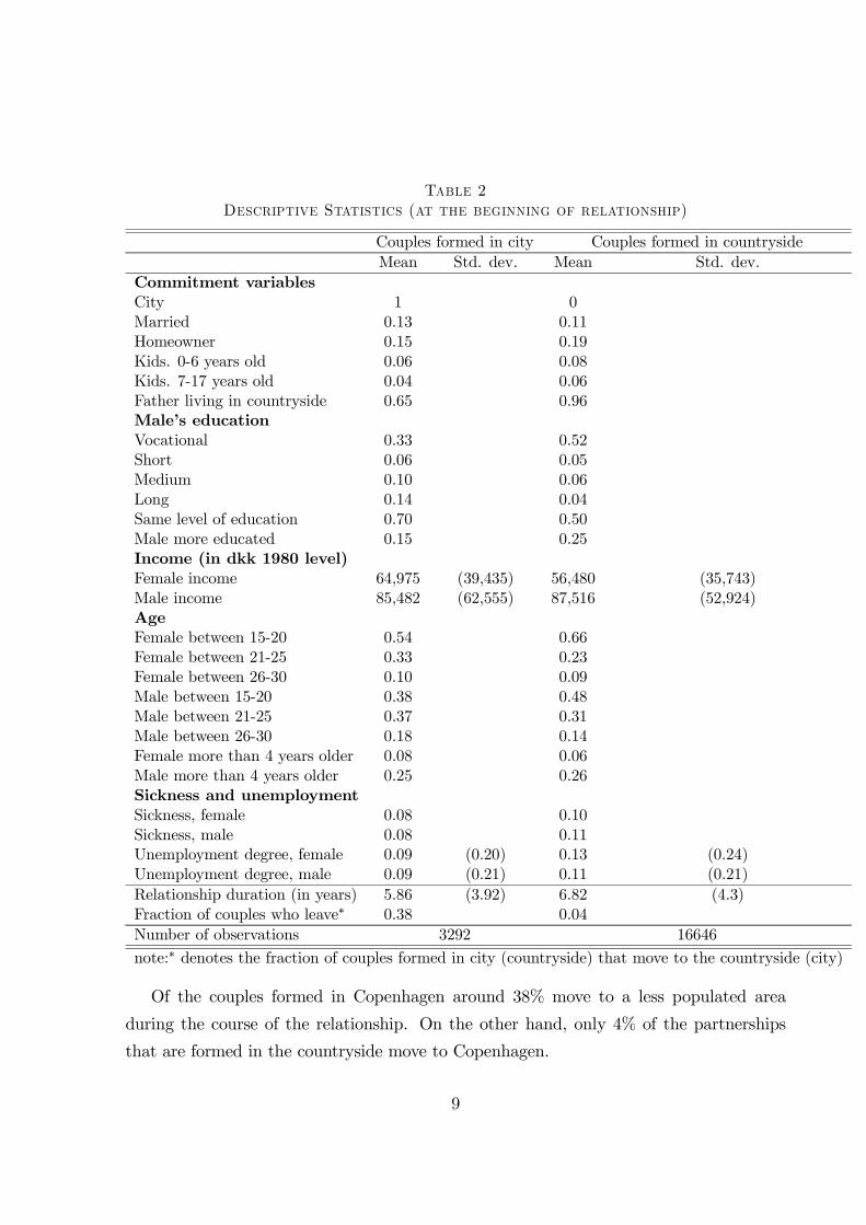
T���� 2D��������� S�������� (�� ��� ���� � � � ������ ����)
Couples formed in city Couples formed in countryside
Mean Std. dev. Mean Std. dev.
Commitment variablesCity 1 0Married 0.13 0.11Homeowner 0.15 0.19Kids. 0-6 years old 0.06 0.08Kids. 7-17 years old 0.04 0.06Father living in countryside 0.65 0.96Male’s educationVocational 0.33 0.52Short 0.06 0.05Medium 0.10 0.06Long 0.14 0.04Same level of education 0.70 0.50Male more educated 0.15 0.25Income (in dkk 1980 level)Female income 64,975 (39,435) 56,480 (35,743)Male income 85,482 (62,555) 87,516 (52,924)AgeFemale between 15-20 0.54 0.66Female between 21-25 0.33 0.23Female between 26-30 0.10 0.09Male between 15-20 0.38 0.48Male between 21-25 0.37 0.31Male between 26-30 0.18 0.14Female more than 4 years older 0.08 0.06Male more than 4 years older 0.25 0.26Sickness and unemploymentSickness, female 0.08 0.10Sickness, male 0.08 0.11Unemployment degree, female 0.09 (0.20) 0.13 (0.24)Unemployment degree, male 0.09 (0.21) 0.11 (0.21)
Relationship duration (in years) 5.86 (3.92) 6.82 (4.3)Fraction of couples who leave∗ 0.38 0.04
Number of observations 3292 16646
note:∗ denotes the fraction of couples formed in city (countryside) that move to the countryside (city)
Of the couples formed in Copenhagen around 38% move to a less populated area
during the course of the relationship. On the other hand, only 4% of the partnerships
that are formed in the countryside move to Copenhagen.
9
3.2 Empirical Model
In order to investigate the effect of locating in a given area on the dissolution risk we
estimate a duration model where the random variable is the time spent in a given rela-
tionship. Since the location decision is potentially endogenous to the dissolution risk, our
goal is to disentangle the commitment effect from the sorting effect. First, we apply the
timing-of-event model of Abbring and van den Berg (2003). We estimate the process of
dissolution simultaneously with the process of moving to a less populated area allowing
the two processes to be interdependent through the error structure. Second, we use an
exclusionary restriction to strengthen identification. We assume that the moving process
starts at the beginning of the relationship.
3.2.1 Timing-of-events method
The timing-of-events method enables us to identify the causal effect of location choice on
the dissolution rate under some well-defined assumptions which we discuss below. The
estimation strategy requires simultaneous modelling of the divorce rate and the moving
hazard. Let Tr(elationship) and Tm(ove) denote the duration of a relationships and the du-
ration till the agent moves in or out of a city. Both are continuous nonnegative random
variables. We allow Tr and Tm to interact through correlation of unobservables or through
a possible treatment effect of moving in or out of the city. Suppose for example that each
period, the couple draws an r =(utility in city/ utility in countryside), where r depends
on for example job market opportunities. Let the marriage quality be given by q ∈ [0, 1].
Then, the optimal strategy is to define a reservation value r∗(q) above which the couple
moves to the city. Then Tm depends on the quality of marriage but not in a deterministic
way. This randomness is necessary for identification. We assume further that all individ-
ual differences in the joint distribution of the processes can be characterized by observed
explanatory variables, x, and unobserved variables, v. The moving incidence and the exit
rate out of marriage are characterized by the moments at which they occur, and we are
interested in the effect of the realization of Tm on the distribution of Tr. The distributions
of the random variables are expressed in terms of their hazard rates hm(t|xm,t, vm) and
hr(t|tm, xr,t, vr). Conditional on x and v, we can therefore ascertain that the realization
of Tm affects the shape of the hazard of Tr from tm onwards in a deterministic way. This
independence assumption implies that the causal effect is captured by the effect of tm on
10
hr(t|tm, xr,t, vr) for t > tm. This rules out that tm affects hr(t|tm, xr,t, vr) for t ≤ tm, i.e.
anticipation of the move has no effect on the relationship hazard. This assumption will
be falsified if one or both partners stop searching in the anticipation period before moving
to the city or searches extra hard in the anticipation period before moving to the coun-
tryside. However, we justify the use of the model by the fact that the time span between
the moment at which the anticipation occurs and the moment that the actual move takes
place is relatively short compared with the duration of a marriage (the average duration
of relationships is approximately 6.7 years in our sample while the average time to find
a house is only a few months). This implies that the potential bias from anticipation is
small.
Given the independence and no anticipation assumptions, the causal effect of moving
on the divorce rate is identified by a mixed proportional hazard model. That is, it is a
product of a function of time spent in the given state (the baseline hazard), a function of
observed time-varying characteristics, xt, and a function of unobserved characteristics, v
h (t|xt, v) = λ (t) · ϕ (xt, v) ,
where λ (t) specified as exp(λm(t)) is the baseline hazard and ϕ (xt, v) is the scaling
function specified as exp(β′xt + v). More specifically the system of equations is:
hm(t|xm,t, vm) = exp(β′
mxm,t + λm(t) + vm) (1)
hr(t|tm, xr,t, vr) = exp(β′
rxr,t + δD(tm) + λr(t) + vr),
where D(tm) is a time-varying indicator variable taking the value 0 before the couple
moves, and 1 after the couple moves.
Intuitively, the timing-of-events method uses variation in marriage duration and in du-
ration until moving (conditional on observed characteristics) to identify the unobserved
heterogeneity distribution. The selection or sorting effect is captured by a positive corre-
lation between vr and vm while the causal effect of living in the city on marriage duration
is captured by the effect of the time spent outside the city conditional on the observables
and vr and vm. If couples who move to the city divorce fast, irrespective of how long
they lived outside the city there is a causal effect of living in the city on the divorce rate.
Alternatively, if only the couples who move to the city just after marriage divorce faster
while the ones who move later do not divorce faster, there is a sorting effect. The most
11
stable relationships are more likely to remain in the countryside for a long time because
they are more likely to have kids or prefer to spend lots of time together while the rel-
atively unstable relationships move to the city fast. This requires however that there is
no interaction between marriage quality and treatment. If for example living in the city
causes bad marriages to dissolve faster this also implies a positive correlation between
vr and vm. In that case, if we would randomly pick a treatment group of 1000 couples
from the countryside and place them in the city we would find a positive treatment effect
caused by the unstable relations who divorce faster in the city than in the countryside.
Abbring and Van den Berg (2003) show that under further proportionality assumptions a
cross effect of marriage quality and the treatments (city and countryside) is identified by
allowing the unobserved characteristics of the marriage quality νr to be different for the
movers and the non movers. The time varying piecewise constant duration effect is then
informative on the city effect. We do not travel this avenue because the assumption of
independence between observables and non-observables after the move cannot be justified.
Alternatively, we impose an exclusionary restriction in the moving equation (this iden-
tification strategy is along the lines of e.g. Lillard (1993)). Specifically, we include as an
extra explanatory variable in the moving hazard -an indicator variable that takes the
value 1 if the father of one of the individuals in a given couple currently lives in the
countryside- assuming that this variable does not affect the dissolution risk but it does
affect the location of the couple. For the Likelihood function we refer to the appendix.
4 Results
Since the quality of a relationship may depend on the location of the marriage -agents
who met in a city could have been more choosy because of the higher contact rate αC-
we report the results separately for the subset of relationships that are formed in the city
and those that are formed in the countryside.
The variables of interest are the commitment variables: being married, whether one
owns a house, having young kids, and having older kids. The latter distinction is important
because the cost of divorce is larger for young kids. Of particular interest in this study is
the time-varying indicator variable that denotes whether the couple is currently living in
the city or in the countryside. In addition to this variable we also condition on the usual
12
suspects in the divorce literature (see e.g. Svarer (2004)). We only report the coefficients
for the commitment variables here. In Table 3 and 4 below, we present three sets of
results for partnerships that were initiated in the city and the countryside, respectively.
First, we show the results for a model where we do not model the moving decision (model
1). Second, we take the moving decision into account and use the timing-of-event model
to address the potential endogeneity of moving in relation to the dissolution risk (model
2). Third, we use as exclusionary restriction an indicator variable that takes the value
1 if the father of one of the individuals in a given couple lives in the countryside and 0
otherwise (model 3). Specifically, we include this variable in the moving hazard equation.
13
T���� 3
R������ �� �������� ������ �� ������ ����� ����� � ��� �� 5
Model 1 Model 2 Model 3
Timing-of-event T-o-E and IV
Coeff. S.E. Coeff. S.E. Coeff. S.E.
Countryside -0.264∗ 0.077 -0.121 0.136 -0.146 0.135
Married -1.499∗ 0.113 -1.474∗ 0.113 -1.499∗ 0.114
Kids 0-6 yrs old -0.325∗ 0.070 -0.319∗ 0.071 -0.320∗ 0.071
Kids 7-17 yrs old 0.013 0.102 -0.009 0.101 -0.008 0.102
Homeowner -0.233∗ 0.084 -0.288∗ 0.088 -0.293∗ 0.089
Father living
in countryside∗∗ 0.660∗ 0.090
Corr(vm, vr)∗∗∗ -0.209∗ 0.073 -0.190∗ 0.070
# couples 3292 3292 3292
Log likelihood -4409 -7737 -7713
Note: ∗ denotes significant different from 0 at the 5% level. ∗∗ gives the results from the
moving hazard. ∗∗∗The standard error for the correlation coefficient has been calculated
based on 1,000 drawings from the multivariate normal distribution with matrix set equal
to the estimated parameter vector and covariance matrix.
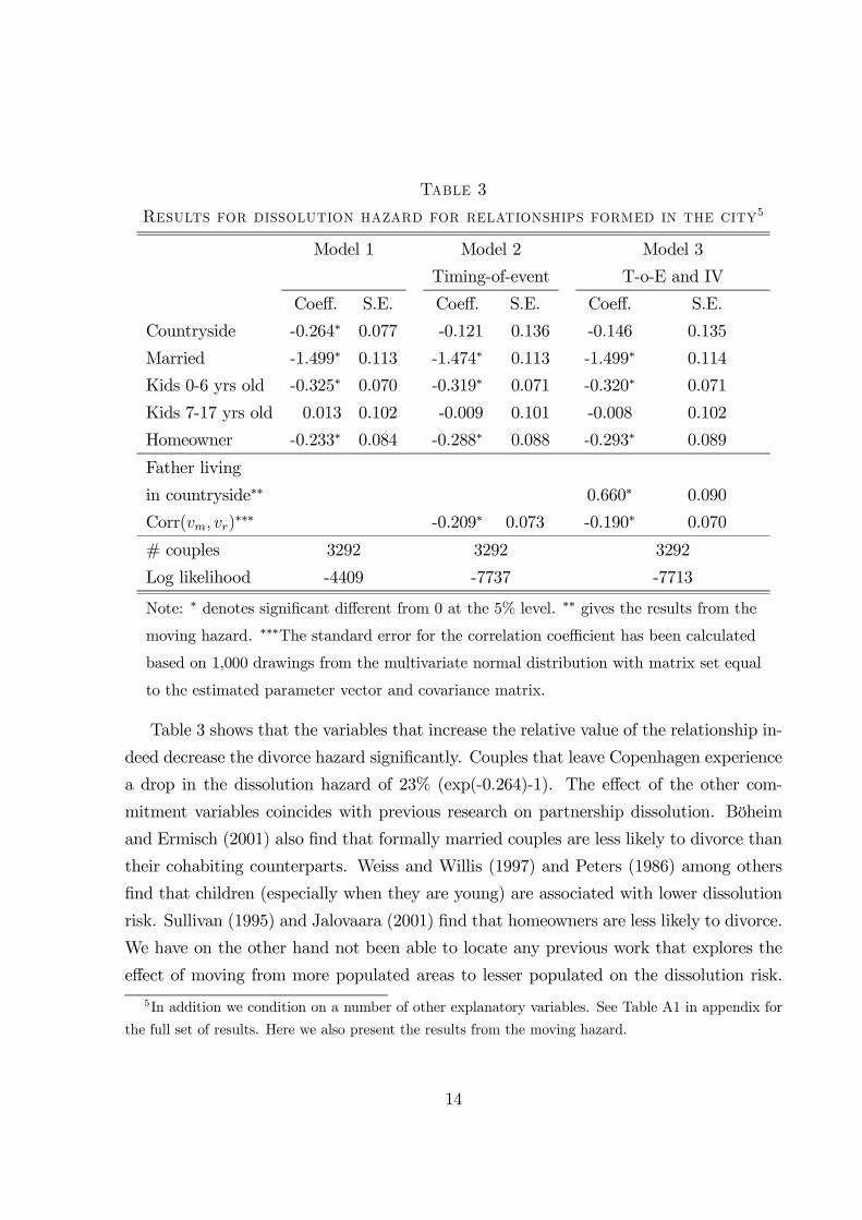
Table 3 shows that the variables that increase the relative value of the relationship in-
deed decrease the divorce hazard significantly. Couples that leave Copenhagen experience
a drop in the dissolution hazard of 23% (exp(-0.264)-1). The effect of the other com-
mitment variables coincides with previous research on partnership dissolution. Böheim
and Ermisch (2001) also find that formally married couples are less likely to divorce than
their cohabiting counterparts. Weiss and Willis (1997) and Peters (1986) among others
find that children (especially when they are young) are associated with lower dissolution
risk. Sullivan (1995) and Jalovaara (2001) find that homeowners are less likely to divorce.
We have on the other hand not been able to locate any previous work that explores the
effect of moving from more populated areas to lesser populated on the dissolution risk.
5In addition we condition on a number of other explanatory variables. See Table A1 in appendix for
the full set of results. Here we also present the results from the moving hazard.
14
Although the fact that the divorce risk is lower in rural areas has also been observed by
Peters (1986) and Jalovaara (2001).
The results presented in model 2 suggest that moving to the countryside is not an
exogenous event in relation to the dissolution process. Indeed, the significant effect of
leaving Copenhagen vanishes once we model the moving decision simultaneously with
the dissolution process. Taken at face value this implies that based on unobservable
factors, the stable relationships are more likely to leave Copenhagen and this association
is what drives the findings of model 1. This is captured by the correlation between the
unobserved heterogeneity terms in the moving hazard and the dissolution hazard. This
correlation is significantly negative. As we argued before, this could also be caused by an
interaction between marriage quality and living in the city (cities have a causal effect on
dissolution of bad marriages). Model 3, where we introduce an exclusionary restriction
in the moving equation suggests however that this is not the case. Couples where at
least one partner has a father currently living in the countryside have a much higher
moving probability. In fact, the hazard rate out of Copenhagen is 93% higher for these
couples. Assuming that father’s location is unrelated to marriage stability and assuming
that the effect of location choice on father’s location is independent of marriage quality
this variable randomizes locations of couples (irrespective of marriage quality). With this
exclusion restriction we find no significant effect of living in the countryside on the divorce
hazard. Moreover, we show in Table A1 (in appendix) that the moving hazard is higher
for couples that also invest in the other commitment variables like becoming homeowner,
having young children and being formally married. This suggests that also in terms of
observables, the stable relationships are more likely to move to the countryside. We do
want to stress however that we use those variables mainly as controls and do not want to
give them a structural interpretation because of endogeneity problems.
The process of moving to a new location is a stressful event. To what extent does this
affect our divorce rate? If we assume that the process of moving can only have an effect
on the hazard rate in the first 2 years we can control for it by allowing for (piecewise
constant) time varying treatment effects of the moving variable in the dissolution hazard.
We do however not find significant time varying effects of moving on the dissolution hazard
and conclude that this exercise does not change our main findings presented in Table 3.
Moreover, below we also look at the reverse movement from countryside to city and find
15
that allowing for sorting results in an insignificant city effect.
We do not consider the exogeneity status of the other commitment variables in this
study. In a related study, Svarer and Verner (2006) take a closer look at children. They
find that couples that are less prone to end their relationship are more likely to get
children. Since couples with children are more likely to leave the city and are also more
likely to buy a house this suggests indeed that stable relationships are more likely to
engage in various forms of commitment.
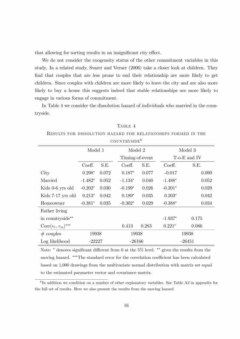
In Table 4 we consider the dissolution hazard of individuals who married in the coun-
tryside.
T���� 4
R������ �� �������� ������ �� ������ ����� ����� � ���
� �� ����6
Model 1 Model 2 Model 3
Timing-of-event T-o-E and IV
Coeff. S.E. Coeff. S.E. Coeff. S.E.
City 0.298∗ 0.072 0.187∗ 0.077 -0.017 0.099
Married -1.482∗ 0.052 -1.134∗ 0.040 -1.488∗ 0.052
Kids 0-6 yrs old -0.202∗ 0.030 -0.199∗ 0.026 -0.201∗ 0.029
Kids 7-17 yrs old 0.213∗ 0.042 0.189∗ 0.035 0.203∗ 0.042
Homeowner -0.381∗ 0.035 -0.302∗ 0.029 -0.388∗ 0.034
Father living
in countryside∗∗ -1.937∗ 0.175
Corr(vr, vm)∗∗∗ 0.413 0.283 0.221∗ 0.086
# couples 19938 19938 19938
Log likelihood -22227 -26166 -26451
Note: ∗ denotes significant different from 0 at the 5% level. ∗∗ gives the results from the
moving hazard. ∗∗∗The standard error for the correlation coefficient has been calculated
based on 1,000 drawings from the multivariate normal distribution with matrix set equal
to the estimated parameter vector and covariance matrix.
6In addition we condition on a number of other explanatory variables. See Table A2 in appendix for
the full set of results. Here we also present the results from the moving hazard.
16
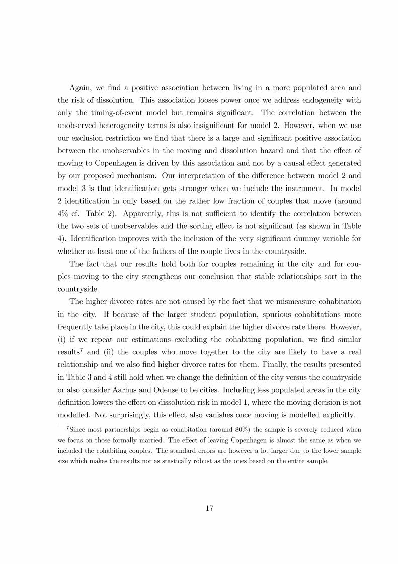
Again, we find a positive association between living in a more populated area and
the risk of dissolution. This association looses power once we address endogeneity with
only the timing-of-event model but remains significant. The correlation between the
unobserved heterogeneity terms is also insignificant for model 2. However, when we use
our exclusion restriction we find that there is a large and significant positive association
between the unobservables in the moving and dissolution hazard and that the effect of
moving to Copenhagen is driven by this association and not by a causal effect generated
by our proposed mechanism. Our interpretation of the difference between model 2 and
model 3 is that identification gets stronger when we include the instrument. In model
2 identification in only based on the rather low fraction of couples that move (around
4% cf. Table 2). Apparently, this is not sufficient to identify the correlation between
the two sets of unobservables and the sorting effect is not significant (as shown in Table
4). Identification improves with the inclusion of the very significant dummy variable for
whether at least one of the fathers of the couple lives in the countryside.
The fact that our results hold both for couples remaining in the city and for cou-
ples moving to the city strengthens our conclusion that stable relationships sort in the
countryside.
The higher divorce rates are not caused by the fact that we mismeasure cohabitation
in the city. If because of the larger student population, spurious cohabitations more
frequently take place in the city, this could explain the higher divorce rate there. However,
(i) if we repeat our estimations excluding the cohabiting population, we find similar
results7 and (ii) the couples who move together to the city are likely to have a real
relationship and we also find higher divorce rates for them. Finally, the results presented
in Table 3 and 4 still hold when we change the definition of the city versus the countryside
or also consider Aarhus and Odense to be cities. Including less populated areas in the city
definition lowers the effect on dissolution risk in model 1, where the moving decision is not
modelled. Not surprisingly, this effect also vanishes once moving is modelled explicitly.
7Since most partnerships begin as cohabitation (around 80%) the sample is severely reduced when
we focus on those formally married. The effect of leaving Copenhagen is almost the same as when we
included the cohabiting couples. The standard errors are however a lot larger due to the lower sample
size which makes the results not as stastically robust as the ones based on the entire sample.
17
5 Concluding remarks
Is moving to the countryside a credible commitment device for couples? In this paper,
we investigate whether lowering the arrival rate of potential marriage partners by moving
to a less populated area lowers the divorce rate for a sample of Danish couples. We find,
using the timing-of-events model of Abbring and van den Berg (2003), that conditional
on location of marriage, the divorce risks are higher in the city but that this is mainly
caused by sorting of relatively stable relationships in the countryside. This is confirmed
by using an exclusion restriction. Our main conclusion is that moving to the countryside
is not a cheap way to prolong relationships.
References
[1] A���� �, J. � � G. �� �� B��� (2003). “The Non-Parametric Identification
of Treatment Effects in Duration Models”, Econometrica, 71, 1491-1517.
[2] B�&��, G., E.M. L� ��� � � R. T. M����� (1977). “An Economic Analysis
of Marital Instability”, Journal of Political Economy, 85(6), 1141-1187.
[3] B� ���, N.G, A.K. B�� � � D.E. B�� (1988). “Commitment and the
Modern Union: Assessing the Link Between Premarital Cohabitation and Subsequent
Marital Stability”, American Sociological Review, 53, 127-138.
[4] B������, K., R. I��� � � RW����� (2004). “Unstable Relationships”, Frontiers
of Macroeconomics, 1 (1), Article 1.
[5] B.����, R. � � J.E����� (2001). “Partnership Dissolution in the UK - the Role
of Economic Circumstances”, Oxford Bulletin of Economics and Statistics, 63, 2,
197-208.
[6] C�������, P.A., M. I ��� � � Y. W���� (2005). “Marriage Markets, Divorce
and Intra-household Allocations”, mimeo, Columbia University.
[7] C� �����, T. (2003). “A Search Model of Marriage and Divorce”, Review of Eco-
nomic Dynamics, 6: 135-55.
18
[8] D��2� &�, S. (2005). “A Generalized Model of Commitment”, Mathematical Social
Science, Forthcoming.
[9] F����, R. (2002). “Prelude to Marriage or Alternative to Marriage? A Social
Demographic Look at Cohabitation in the U.S.”, Journal of Law and Family Studies,
4(1), 91-104.
[10] G������, P.A., M. S����� � � T���� �� C.N. (2005). “Marriage and the City”,
Working Paper 2005-01, Department of Economics, University of Aarhus.
[11] J�������, M. (2001). “Socio-Economic Status and Divorce in First Marriages in
Finland 1991-93”, Population Studies, 55, 119-133.
[12] K�����, N.M. (1990). “Econometric Methods for Grouped Duration Data”. In:
Panel Data and Labour Market Studies, North-Holland.
[13] L������, L.A. (1993). “Simultaneous Equations for Hazards — Marriage Duration
and Fertility Timing”, Journal of Econometrics, 56, 189-217.
[14] M������, A. (2005). “Marriage, Commitment and Divorce in a Matching Model
with Differential Aging”, Draft, University of Albany, SUNY.
[15] P�����, E. H. (1986). “Marriage and Divorce: Informational Constraints and Pri-
vate Contracting”, American Economic Review, 76(3), 437-454.
[16] R������, C.E. (1980). “Commitment and Satisfaction in Romantic Associations:
A Test of the Investment Model”, Journal of Experimental Social Psychology, 16,
172-186.
[17] S������ , T. (1995). “Ex Ante Divorce Probability and Investment in Marital-
Specific Assets: An Application to Home Ownership”, Working Paper 95-5, Univer-
sity of Maryland, Department of Economics.
[18] S�����, M. (2004). “Is Your Love in Vain? Another Look at Premarital Cohabita-
tion and Divorce”, Journal of Human Resources, 39(2), 523-536.
[19] S�����, M. � � M. V�� �� (2006). “Do Children Stabilize Danish Marriages?”,
Forthcoming in Journal of Population Economics.
19
[20] �� �� B���, G. (2001). “Duration Models: Specification, Identification, and
Multiple Durations”, in J.J. Heckman and E. Leamer, eds., Handbook of Economet-
rics, Vol. V, North Holland, Amsterdam.
[21] W����, Y. � � R.J. W����� (1997). “Match Quality, New Information, and Marital
Dissolution”, Journal of Labor Economics, 15(1), S293-S329.
20
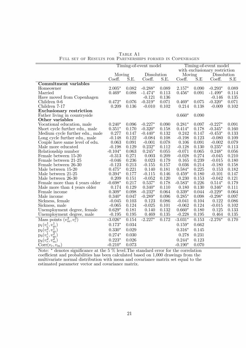
T���� A1F��� ��� � R������ �� P��� ������� ����� � C�� ����
Timing-of-event model Timing-of-event modelwith exclusionary restriction
Moving Dissolution Moving DissolutionCoeff. S.E. Coeff. S.E. Coeff. S.E Coeff. S.E
Commitment variablesHomeowner 2.005∗ 0.082 -0.288∗ 0.089 2.157∗ 0.090 -0.293∗ 0.089Married 0.469∗ 0.088 -1.474∗ 0.113 0.456∗ 0.091 -1.499∗ 0.114Have moved from Copenhagen -0.121 0.136 -0.146 0.135Children 0-6 0.472∗ 0.076 -0.319∗ 0.071 0.469∗ 0.075 -0.320∗ 0.071Children 7-17 0.209 0.136 -0.010 0.102 0.214 0.138 -0.009 0.102Exclusionary restrictionFather living in countryside 0.660∗ 0.090Other variablesVocational education, male 0.240∗ 0.096 -0.227∗ 0.090 0.281∗ 0.097 -0.227∗ 0.091Short cycle further edu., male 0.351∗ 0.170 -0.320∗ 0.158 0.414∗ 0.178 -0.345∗ 0.160Medium cycle further edu., male 0.277 0.147 -0.440∗ 0.132 0.242 0.147 -0.453∗ 0.133Long cycle further edu., male -0.148 0.122 -0.084 0.108 -0.198 0.123 -0.080 0.109Couple have same level of edu. 0.063 0.091 -0.001 0.078 0.106 0.091 -0.002 0.079Male more educated -0.198 0.129 0.232∗ 0.112 -0.128 0.130 0.235∗ 0.113Relationship number -0.104∗ 0.063 0.245∗ 0.055 -0.071 0.065 0.248∗ 0.056Female between 15-20 -0.313 0.271 0.003 0.209 -0.028 0.274 -0.045 0.210Female between 21-25 -0.046 0.236 0.023 0.179 0.165 0.239 -0.015 0.180Female between 26-30 -0.123 0.213 -0.155 0.157 0.036 0.214 -0.180 0.158Male between 15-20 0.475∗ 0.221 0.140 0.181 0.584∗ 0.225 0.153 0.182Male between 21-25 0.394∗ 0.177 -0.115 0.146 0.459∗ 0.180 -0.101 0.147Male between 26-30 0.209 0.151 -0.052 0.120 0.230 0.153 -0.042 0.121Female more than 4 years older -0.698∗ 0.217 0.537∗ 0.178 -0.583∗ 0.226 0.514∗ 0.179Male more than 4 years older 0.174 0.129 0.340∗ 0.110 0.180 0.130 0.346∗ 0.111Female income 0.309∗ 0.098 -0.232∗ 0.064 0.339∗ 0.044 -0.229∗ 0.064Male income 0.340∗ 0.047 -0.289∗ 0.096 0.285∗ 0.098 -0.298∗ 0.097Sickness, female -0.045 0.103 0.123 0.086 -0.041 0.104 0.122 0.086Sickness, male -0.065 0.124 -0.025 0.101 -0.062 0.124 -0.015 0.102Unemployment degree, female 0.629∗ 0.181 0.140 0.132 0.660∗ 0.180 0.125 0.133Unemployment degree, male -0.195 0.195 0.469 0.135 -0.228 0.195 0.464 0.135Mass points (v2m, v
2r ) -3.026∗ 0.154 -2.227∗ 0.172 -3.031∗ 0.153 -2.276∗ 0.170
p1(v1r , v
1m) 0.173∗ 0.034 0.159∗ 0.662
p2(v2r , v
1m) 0.330∗ 0.029 0.316∗ 0.145
p3(v1r , v
2m) 0.274∗ 0.030 0.278 0.231
p4(v2r , v
2m) 0.223∗ 0.026 0.244∗ 0.123
Corr(vr, vm) -0.210∗ 0.073 -0.190∗ 0.070
Note: ∗ denotes significance at the 5 % level.The standard error for the correlationcoefficient and probabilities has been calculated based on 1,000 drawings from themultivariate normal distribution with mean and covariance matrix set equal to theestimated parameter vector and covariance matrix.
21
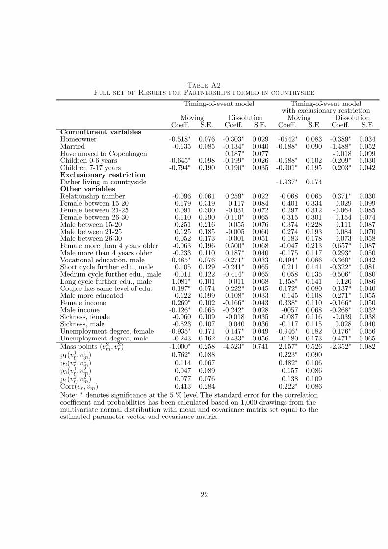
T���� A2F��� ��� � R������ �� P��� ������� ����� � � �� ����
Timing-of-event model Timing-of-event modelwith exclusionary restriction
Moving Dissolution Moving DissolutionCoeff. S.E. Coeff. S.E. Coeff. S.E Coeff. S.E
Commitment variablesHomeowner -0.518∗ 0.076 -0.303∗ 0.029 -0542∗ 0.083 -0.389∗ 0.034Married -0.135 0.085 -0.134∗ 0.040 -0.188∗ 0.090 -1.488∗ 0.052Have moved to Copenhagen 0.187∗ 0.077 -0.018 0.099Children 0-6 years -0.645∗ 0.098 -0.199∗ 0.026 -0.688∗ 0.102 -0.209∗ 0.030Children 7-17 years -0.794∗ 0.190 0.190∗ 0.035 -0.901∗ 0.195 0.203∗ 0.042Exclusionary restrictionFather living in countryside -1.937∗ 0.174Other variablesRelationship number -0.096 0.061 0.259∗ 0.022 -0.068 0.065 0.371∗ 0.030Female between 15-20 0.179 0.319 0.117 0.084 0.401 0.334 0.029 0.099Female between 21-25 0.091 0.300 -0.031 0.072 0.297 0.312 -0.064 0.085Female between 26-30 0.110 0.290 -0.110∗ 0.065 0.315 0.301 -0.154 0.074Male between 15-20 0.251 0.216 0.055 0.076 0.374 0.228 0.111 0.087Male between 21-25 0.125 0.185 -0.005 0.060 0.274 0.193 0.084 0.070Male between 26-30 0.052 0.173 -0.001 0.051 0.183 0.178 0.073 0.058Female more than 4 years older -0.063 0.196 0.500∗ 0.068 -0.047 0.213 0.657∗ 0.087Male more than 4 years older -0.233 0.110 0.187∗ 0.040 -0.175 0.117 0.293∗ 0.050Vocational education, male -0.485∗ 0.076 -0.271∗ 0.033 -0.494∗ 0.086 -0.360∗ 0.042Short cycle further edu., male 0.105 0.129 -0.241∗ 0.065 0.211 0.141 -0.322∗ 0.081Medium cycle further edu., male -0.011 0.122 -0.414∗ 0.065 0.058 0.135 -0.506∗ 0.080Long cycle further edu., male 1.081∗ 0.101 0.011 0.068 1.358∗ 0.141 0.120 0.086Couple has same level of edu. -0.187∗ 0.074 0.222∗ 0.045 -0.172∗ 0.080 0.137∗ 0.040Male more educated 0.122 0.099 0.108∗ 0.033 0.145 0.108 0.271∗ 0.055Female income 0.269∗ 0.102 -0.166∗ 0.043 0.338∗ 0.110 -0.166∗ 0.050Male income -0.126∗ 0.065 -0.242∗ 0.028 -0057 0.068 -0.268∗ 0.032Sickness, female -0.060 0.109 -0.018 0.035 -0.087 0.116 -0.039 0.038Sickness, male -0.623 0.107 0.040 0.036 -0.117 0.115 0.028 0.040Unemployment degree, female -0.935∗ 0.171 0.147∗ 0.049 -0.946∗ 0.182 0.176∗ 0.056Unemployment degree, male -0.243 0.162 0.433∗ 0.056 -0.180 0.173 0.471∗ 0.065Mass points (v2m, v
2r ) -1.000∗ 0.258 -4.523∗ 0.741 2.157∗ 0.526 -2.352∗ 0.082
p1(v1r , v
1m) 0.762∗ 0.088 0.223∗ 0.090
p2(v2r , v
1m) 0.114 0.067 0.482∗ 0.106
p3(v1r , v2m) 0.047 0.089 0.157 0.086
p4(v2r , v2m) 0.077 0.076 0.138 0.109
Corr(vr, vm) 0.413 0.284 0.222∗ 0.086Note: ∗ denotes significance at the 5 % level.The standard error for the correlationcoefficient and probabilities has been calculated based on 1,000 drawings from themultivariate normal distribution with mean and covariance matrix set equal to theestimated parameter vector and covariance matrix.
22
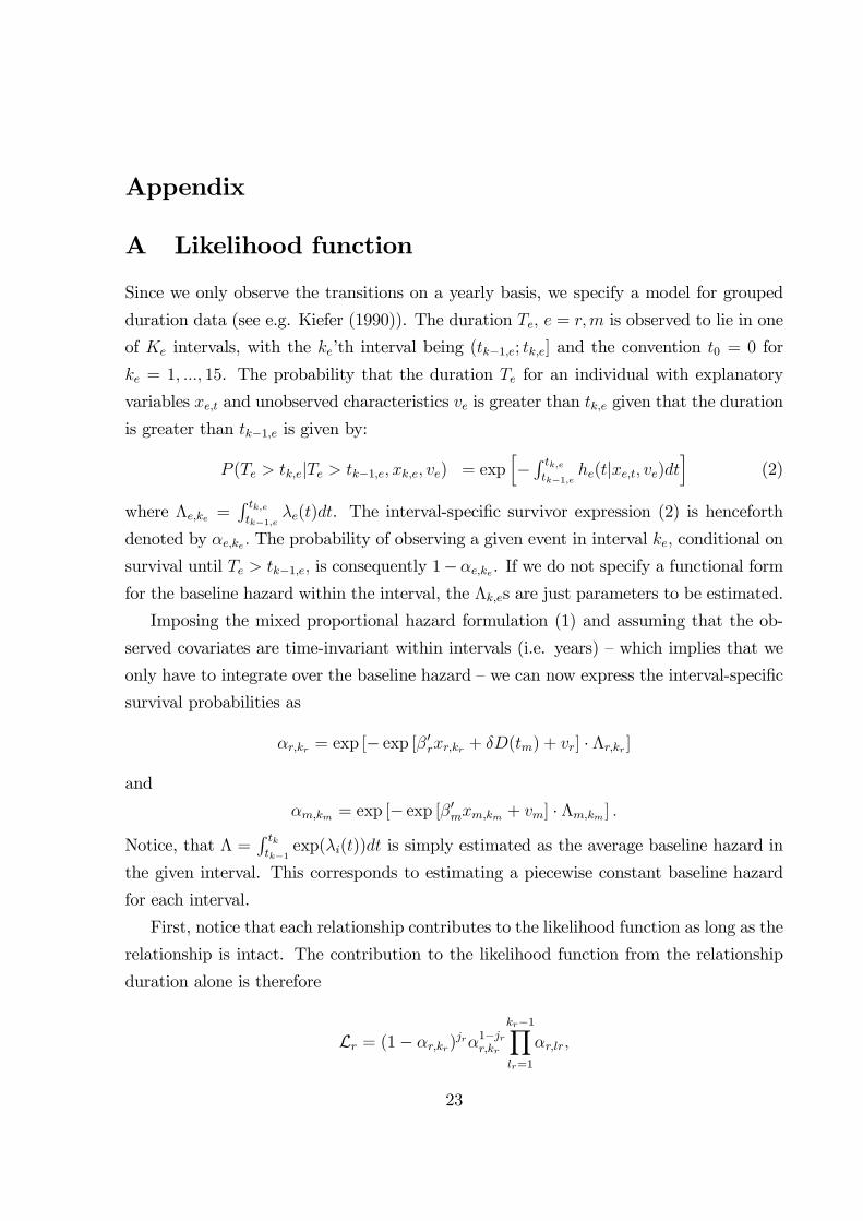
Appendix
A Likelihood function
Since we only observe the transitions on a yearly basis, we specify a model for grouped
duration data (see e.g. Kiefer (1990)). The duration Te, e = r,m is observed to lie in one
of Ke intervals, with the ke’th interval being (tk−1,e; tk,e] and the convention t0 = 0 for
ke = 1, ..., 15. The probability that the duration Te for an individual with explanatory
variables xe,t and unobserved characteristics ve is greater than tk,e given that the duration
is greater than tk−1,e is given by:
P (Te > tk,e|Te > tk−1,e, xk,e, ve) = exp[−∫ tk,etk−1,e
he(t|xe,t, ve)dt]
(2)
where Λe,ke =∫ tk,etk−1,e
λe(t)dt. The interval-specific survivor expression (2) is henceforth
denoted by αe,ke . The probability of observing a given event in interval ke, conditional on
survival until Te > tk−1,e, is consequently 1−αe,ke. If we do not specify a functional form
for the baseline hazard within the interval, the Λk,es are just parameters to be estimated.
Imposing the mixed proportional hazard formulation (1) and assuming that the ob-
served covariates are time-invariant within intervals (i.e. years) — which implies that we
only have to integrate over the baseline hazard — we can now express the interval-specific
survival probabilities as
αr,kr = exp [− exp [β′
rxr,kr + δD(tm) + vr] · Λr,kr ]
and
αm,km = exp [− exp [β′
mxm,km + vm] · Λm,km ] .
Notice, that Λ =∫ tktk−1
exp(λi(t))dt is simply estimated as the average baseline hazard in
the given interval. This corresponds to estimating a piecewise constant baseline hazard
for each interval.
First, notice that each relationship contributes to the likelihood function as long as the
relationship is intact. The contribution to the likelihood function from the relationship
duration alone is therefore
Lr = (1− αr,kr)jrα
1−jrr,kr
kr−1∏
lr=1
αr,lr,
23
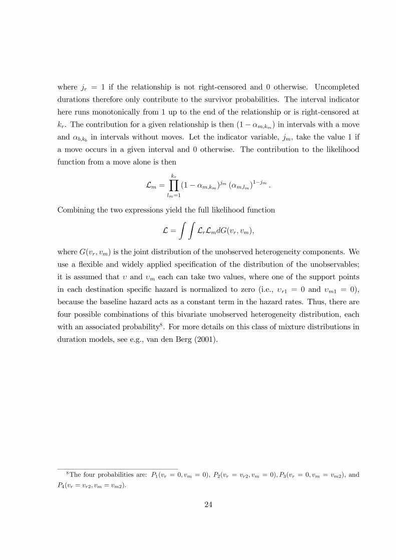
where jr = 1 if the relationship is not right-censored and 0 otherwise. Uncompleted
durations therefore only contribute to the survivor probabilities. The interval indicator
here runs monotonically from 1 up to the end of the relationship or is right-censored at
kr. The contribution for a given relationship is then (1− αm,km) in intervals with a move
and αb,kb in intervals without moves. Let the indicator variable, jm, take the value 1 if
a move occurs in a given interval and 0 otherwise. The contribution to the likelihood
function from a move alone is then
Lm =kr∏
lm=1
(1− αm,km)jm (αm,lm)
1−jm .
Combining the two expressions yield the full likelihood function
L =
∫ ∫LrLmdG(vr, vm),
where G(vr, vm) is the joint distribution of the unobserved heterogeneity components. We
use a flexible and widely applied specification of the distribution of the unobservables;
it is assumed that υ and υm each can take two values, where one of the support points
in each destination specific hazard is normalized to zero (i.e., υr1 = 0 and υm1 = 0),
because the baseline hazard acts as a constant term in the hazard rates. Thus, there are
four possible combinations of this bivariate unobserved heterogeneity distribution, each
with an associated probability8. For more details on this class of mixture distributions in
duration models, see e.g., van den Berg (2001).
8The four probabilities are: P1(vr = 0, vm = 0), P2(vr = vr2, vm = 0), P3(vr = 0, vm = vm2), and
P4(vr = vr2, vm = vm2).
24