Embed Size (px)
Citation preview
SimVAE: Simulator-Assisted Training forInterpretable Generative Models
Akash Srivastava∗MIT-IBM Watson AI Lab
IBM ResearchCambridge, MA
Jessie Rosenberg∗MIT-IBM Watson AI Lab
IBM ResearchCambridge, MA
Dan GutfreundIBM Research
Cambridge, [email protected]
David D. CoxMIT-IBM Watson AI Lab
IBM ResearchCambridge, MA
Abstract
This paper presents a simulator-assisted training method (SimVAE) for variationalautoencoders (VAE) that leads to a disentangled and interpretable latent space.Training SimVAE is a two step process in which first a deep generator network(decoder) is trained to approximate the simulator. During this step the simulator actsas the data source or as a teacher network. Then an inference network (encoder)is trained to invert the decoder. As such, upon complete training, the encoderrepresents an approximately inverted simulator. By decoupling the training ofthe encoder and decoder we bypass some of the difficulties that arise in traininggenerative models such as VAEs and generative adversarial networks (GANs). Weshow applications of our approach in a variety of domains such as circuit design,graphics de-rendering and other natural science problems that involve inferencevia simulation.
1 Introduction
Simulation as a scientific tool is as old as scientific exploration itself. From the ancient Greeks whodrew circles in the sand to discover the connection between radius and circumference, to modernsimulations of complex atomic reactions, protein folding and photo-realistic computer graphics,simulators represent human knowledge in a well-defined symbolic form, crystallizing informationinto models that can generate output data based on particular input specifications. Much of ourprogress in understanding the world relies on developing simulators, often using several of them inconcert to describe larger interconnected systems.
Humans (and animals in general) also distill information from the world, but rather than explicitlyknowing and manipulating precise equations governing e.g. the laws of physics, they have an intuitivesense of physics that allows split second, “good enough” estimates; for instance, even a dog can catcha ball mid-air without explicitly knowing the laws of physics or manipulating equations. Therefore,one might speculate that our brains possess some form of a “simulation engine in the head,” whichdistills knowledge of the world into simpler heuristics that help us in our everyday lives (Lake et al.,2017). Moreover, a desirable feature of such a simplified model would be to allow inference in both
∗Equal Contribution.
Preprint. Under review.
arX
iv:1
911.
0805
1v1
[st
at.M
L]
19
Nov
201
9
the forward and inverse directions of the simulator, in contrast to traditional numerical simulatorswhich are difficult or impossible to invert.
In this paper we address the question of how to distill symbolic mappings modeled by complex andnot necessarily differentiable simulators into neural networks. Classification systems can learn a mapbetween data points and labels, but there is no continuity in the output space and these systems oftencannot generalize well to new types of examples. Generative models understand their domain wellenough to create new examples, they possess smooth mappings over the input-output space, andcan operate probabilistically. However, the latent space typically does not correspond to any human-understandable set of parameters; therefore it is difficult to generate output data with a specified set offeatures. If a larger system needs to take input from multiple domains, all component parts must betrained together end-to-end, since there is no interpretable and standard interface between componentsthat would allow different units to be swapped out or combined in different configurations. In recentyears, a few approaches to address these issues have been proposed (Chen et al., 2016; Higgins et al.,2017; Kulkarni et al., 2015). In Section 3.1 we compare our approach to these works.
Here we present SimVAE, a method for training a variational autoencoder model of a simulator,resulting in both a generator that represents a simplified, probabilistic version of the simulator, andan encoder that is a corresponding probabilistic inverse of the simulator. Though simulators can ingeneral be quite complex and may be discontinuous, a heuristic, smooth version that is invertiblecan be valuable for applications in downstream reasoning tasks, or in technical fields such as circuitdesign, protein folding, and materials design, among others. Such a simplified simulator can also beused as a guide for further detailed inquiry into specific parameter spaces of interest that could takeplace back in the original, more accurate simulation domain.
The SimVAE training method naturally restricts the latent space to be both interpretable and disen-tangled. Note that this does not require orthogonality, and in fact we show example cases where thenatural and interpretable parameters of the simulator are not orthogonal. In this case the SimVAElatent space matches the simulator input space rather than artificially constraining its parameters tobe orthogonal at the cost of reducing accuracy. SimVAE can be trained either in a semi-supervisedmanner using an explicit simulator, which results in a differentiable, probabilistic model and inversemodel of the simulator, or can be trained fully unsupervised by taking the inputs from, for example, aGAN (Goodfellow et al., 2014) or InfoGAN (Chen et al., 2016).
We demonstrate the general applicability of our approach by plugging in several simulators from verydifferent domains such as computer graphics, circuit design and mathematics. This is in contrastto most previous works on learning disentangled representations which focused on understandingimages and scenes.
2 Background
Variational autoencoders (VAE) (Kingma & Welling, 2014) and generative adversarial networks(GAN) (Goodfellow et al., 2014) are two of the most popular state-of-art methods for learning deepgenerative models. Both methods are unsupervised and only need samples {xi}Mi=1 from the datadistribution px to learn a parametric model Gφ (generator) whose distribution qφ matches that ofthe true data px. The distributions are matched using discrepancy measures such as f -divergences(Kullback & Leibler, 1951) or integral probability metrics (Gretton et al., 2012).
In VAEs, Gφ represents a probabilistic function that maps sets of samples from the prior distributionpz over the latent space RK to sets of samples in the observation space RN . In doing so, it additionallyrequires an encoding function (encoder) or an inference network Eθ to parameterise the variationalposterior pθ(z|x), which is trained to approximately invert the mapping of Gφ. VAEs make anassumption about the distribution of the data, which yields a likelihood function. As such they can betrained using stochastic gradient based variational inference. In practice, the VAE training objectiveis a lower bound to the log-likelihood, also referred to as the ELBO:∫Xpx(x) log qφ(x)dx ≥
∫Xpx(x)
[ ∫Zpθ(z|x) log
pzpθ(z|x)
dz +
∫Zpθ(z|x) log qφ(x|z)dz
]dx.
(1)
This ELBO has a unique form, the first term is in fact a negative Kullback–Leibler (KL) divergencebetween the variational posterior and the model prior over the latent space. The second term promotes
2
the likelihood of the observed data under the assumed model φ but it is not always tractable unlikethe first term and is usually estimated using Monte Carlo (MC) estimators. But MC estimator basedtraining increases the variance of the gradients. This increase in variance is controlled using there-parameterisation trick which, in effect, removes the MC sampler from the computation graph. Forexample, using this trick u ∼ N (µ, σ) can be expressed as u = µ+ σ ∗ ε where ε ∼ N (0, 1). Thisgives the final ELBO
Epx [log qφ(x)] ≥ Epx[−KL[pθ(z|x)‖pz] + EN (0,I)[log qφ(x|µθ(x) + σθ(x) ∗ ε)]
]. (2)
Here µθ and σθ are posterior parameters that the encoder function Eθ outputs.
3 Method
In this section we describe the two-step, simulator-assisted training procedure of SimVAE. Weformally define the simulator S : RK 7→ RN as a deterministic black-box function that maps each ithpoint zi ∈ RK from its domain to a unique point xi ∈ RN in its range. Usually, N >> K for mostphysical simulators. In the first step, SimVAE trains a generator Gφ : RK 7→ RN , a Borel measurablefunction, to learn a probabilistic map of the simulator S. In order to achieve this we define Z(z), inthe latent space, and X(x), in the output space, as K and N dimensional random variables. In orderto learn the function S faithfully, Gφ is parameterized with a deep neural network. The training isachieved by minimizing a suitable measure of discrepancy D (depending on the output space of S)on the observations from the two functions on the same input with respect to φ, as shown below:
minφLD(φ) = min
φ
∑i
D[S(zi), Gφ(zi)]. (3)
Since the domain of S is infinite in practice, the optimization problem is solved using mini-batches ina stochastic gradient descent first order optimization method such as ADAM.
Upon successful training of the generator, Gφ ≈ S, the next step in SimVAE is to train an inferencenetwork (encoder, Eθ : RD 7→ RK) to invert the generator, which in turn, if successfully trained,will give an approximate inversion of the simulator and as a result a disentangled and interpretablerepresentation of the latent space. We do that via the following objective:
minθLE(θ) = min
θ
∑i
D[S(zi), Gφ(µEθ (S(zi)))]. (4)
Here, µEθ is the posterior parameters that the encoder output. We emphasize that training the encoderdoes not involve any supervision. Computation is only done on S(zi), a sample in data space, whilethe latent variables zi are hidden. The key point is that while the simulator is typically black-boxand non-differentiable, the generator is a neural network which we control and therefore we canbackpropagate through the network and the latent variables to train the encoder. Note, while we usethe re-parameterization trick here, in general our method does not require it. If it is not used, in thecases where S is a one-to-many map, the encoder will only learn one such mapping.
3.1 Comparison to other related approaches
SimVAE vs. Classification. Having access to a simulator, one could directly train a model of itsinverse via the following objective:
minθLE(θ) = min
θ
∑i
loss[zi, Eθ(S(zi))], (5)
where loss could be any classification loss (e.g. cross entropy) and/or regression loss (e.g. MSE)depending on z’s components. In other words, we could turn the problem into a supervised classi-fication/regression problem. This was done in the past for graphics de-rendering, see for example(Jiajun Wu, 2017a).
3
There are several reasons why our approach of inverting the generator is preferred. First, z can involvemany components which could be very different in nature, turning the problem into a complex multi-task learning problem, where some of the output parameters may be correlated (see the box plotterexample in Section 4.1). Furthermore, the inverse of the simulator could potentially be (and often is)a one-to-many relation (see the RLC or polygon examples in Section 4.1), turning the problem into amulti-label learning problem. Most importantly, while loss functions on the latent/symbolic space areuseful mathematically and are often used for supervised learning, discrepancies in the observablespace, which are the basis for loss functions used to train generative models such as VAE, allowreconstruction of the data distribution and are more natural for humans learning (see Section 5).
SimVAE vs. other disentangled representation learning schemes. In the last few years severalapproaches for learning disentangled representations with generative models have been proposed.Here we survey the ones that are most related to this paper.
We start with three VAE-based approaches. β-VAE (Higgins et al., 2017) is an unsupervised techniquewhich involves constraining the representations to ensure variable independence at the price ofreconstruction accuracy. A hyper-parameter governs that trade-off. We note that the assumptionof latent variables independence does not necessarily hold, see the box plots example in Section4.1. Deep Convolutional Inverse Graphics Network (DC-IGN) (Kulkarni et al., 2015) is a semi-supervised approach for learning interpretable representations of graphics engines. A crucial aspectin training DC-IGN models is the ability to divide the training set into batches in which only one ofthe latent variables varies (e.g. lighting) while all others are fixed. Training proceeds by clampingall the fixed latent variables to their respective means. We note that while this makes sense forgraphics engines, the average of latent variables does not necessarily corresponds to a meaningfuldata point in the observable space (e.g. see our RLC circuits example). (N Siddharth & Torr, 2017)incorporate graphical models to the VAE architecture, imposing assumptions on the interpretablevariables. Naturally, the specific graphical model depends on the use-case and requires a re-design ifthe application changes.
InfoGANs (Chen et al., 2016) learn disentangled representations by regularizing the minimax gamebetween the discriminator and the generator in the GAN framework with an information-theoreticterm which aims to maximize the mutual information between a small set of latent variables and theobserved data. While InfoGANs have shown impressive results on visual data, still as an unsupervisedmethod it can miss latent information that is important in certain contexts. For example, feeding animage of a function curve to an InfoGAN will likely generate a representation capturing appearanceproperties of the curve, but it is unlikely that it will retrieve the Fourier coefficients of the function.In addition, InfoGAN, just like other GAN-based approaches, require a significant amount of trainingwhile balancing the discriminator and the generator to keep the training stable.
Finally, Wu et. al. (Jiajun Wu, 2017b) suggest an approach which combines inference models withgenerative models. However, the models are not trained based on a single simulation but ratherindependently and thus the approach is not as general as the one we suggest here.
In contrast to the previously mentioned works, our method is general and applies to simulators froma plethora of domains. It does not make any assumptions on the prior or posterior distributions, andit avoids some of the difficulties in jointly training competing (as in GANs) or complementing (asin VAE) models. It relies of course, on the existence of a simulator but as we argue, simulators areeverywhere when thinking about them broadly, even the world can be viewed as a simulator (seeSection 5).
4 Experiments
We trained the SimVAE on a variety of simulators, both image-based and purely symbolic, to showthe generality of this training method. We used the ADAM (Kingma & Ba, 2015) optimiser fortraining, with the learning rate set to 0.001 and the other parameters set to their default values inthe Tensorflow framework. All image-based models were trained using the DCGAN architecture(Radford et al. (2016)), and the RLC circuit simulator model was trained using a simple feed-forwardarchitecture. The architecture of the SimVAE is interchangeable depending on the desired task, e.g. aRNN could be used for circuit simulation to capture larger signal spaces, or an autoregressive decodercould be used for image generation tasks to enhance reproduction accuracy.
4
Box plotter
Hand drawn examples
dSpritesPolygon plotter
Fourier transform
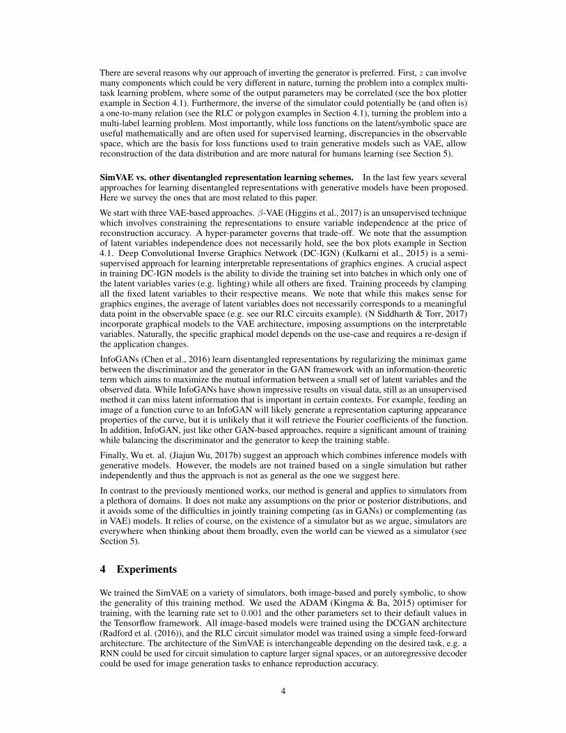
Figure 1: Output of simulator, encoder and generator for image-based models. For each of thefour image-based simulators, random samples are shown of the simulator output X on input Z,the generator output X̄ on the same input Z, the simulator output X on encoder output Z̄, and thegenerator output X̄ on encoder output Z̄, arranged top to bottom in each section. For the Fouriertransform, we also show inference on four hand drawn images (right), excepting the generator X̄from input Z as the input Z is not available in this case.
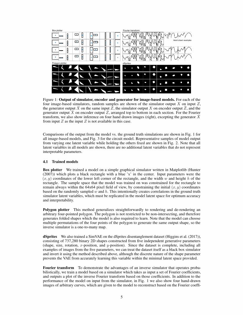
Comparisons of the output from the model vs. the ground truth simulations are shown in Fig. 1 forall image-based models, and Fig. 3 for the circuit model. Representative samples of model outputfrom varying one latent variable while holding the others fixed are shown in Fig. 2. Note that alllatent variables in all models are shown, there are no additional latent variables that do not representinterpretable parameters.
4.1 Trained models
Box plotter We trained a model on a simple graphical simulator written in Matplotlib (Hunter(2007)) which plots a black rectangle with a blue ’x’ in the center. Input parameters were the(x, y) coordinates of the lower left corner of the rectangle, and the width w and height h of therectangle. The sample space that the model was trained on was constrained for the rectangle toremain always within the 64x64 pixel field of view, by constraining the initial (x, y) coordinatesbased on the randomly sampled w and h. This intentionally creates correlations in the ground truthsimulator latent variables, which must be replicated in the model latent space for optimum accuracyand interpretability.
Polygon plotter This method generalizes straightforwardly to rendering and de-rendering anarbitrary four-pointed polygon. The polygon is not restricted to be non-intersecting, and thereforegenerates folded shapes which the model is also required to learn. Note that the model can choosemultiple permutations of the four points of the polygon to generate the same output shape, so theinverse simulator is a one-to-many map.
dSprites We also trained a SimVAE on the dSprites disentanglement dataset (Higgins et al. (2017)),consisting of 737,280 binary 2D shapes constructed from five independent generative parameters(shape, size, rotation, x-position, and y-position). Since the dataset is complete, including allexamples of images from the five parameters, we can treat the dataset itself as a black box simulatorand invert it using the method described above, although the discrete nature of the shape parameterprevents the VAE from accurately learning this variable within the minimal latent space provided.
Fourier transform To demonstrate the advantages of an inverse simulator that operates proba-bilistically, we train a model based on a simulator which takes as input a set of Fourier coefficients,and outputs a plot of the inverse Fourier transform based on those coefficients. In addition to theperformance of the model on input from the simulator, in Fig. 1 we also show four hand-drawnimages of arbitrary curves, which are given to the model to reconstruct based on the Fourier coeffi-
5
Box plotter Fourier transform
Polygon plotter dSprites
Figure 2: Latent transversals. For each of the four image-based simulators, the output of thegenerator upon transversing one latent variable and holding the others fixed is shown for each of thelatent variables. Box plotter: [width, height, x-position, y-position], Fourier transform: [constant, 5cosine coefficients, 5 sine coefficients], Polygon plotter: [(x,y) coordinates for each of four points ofthe polygon], dSprites: [shape, scale, rotation, x-position, y-position].
f0 Q
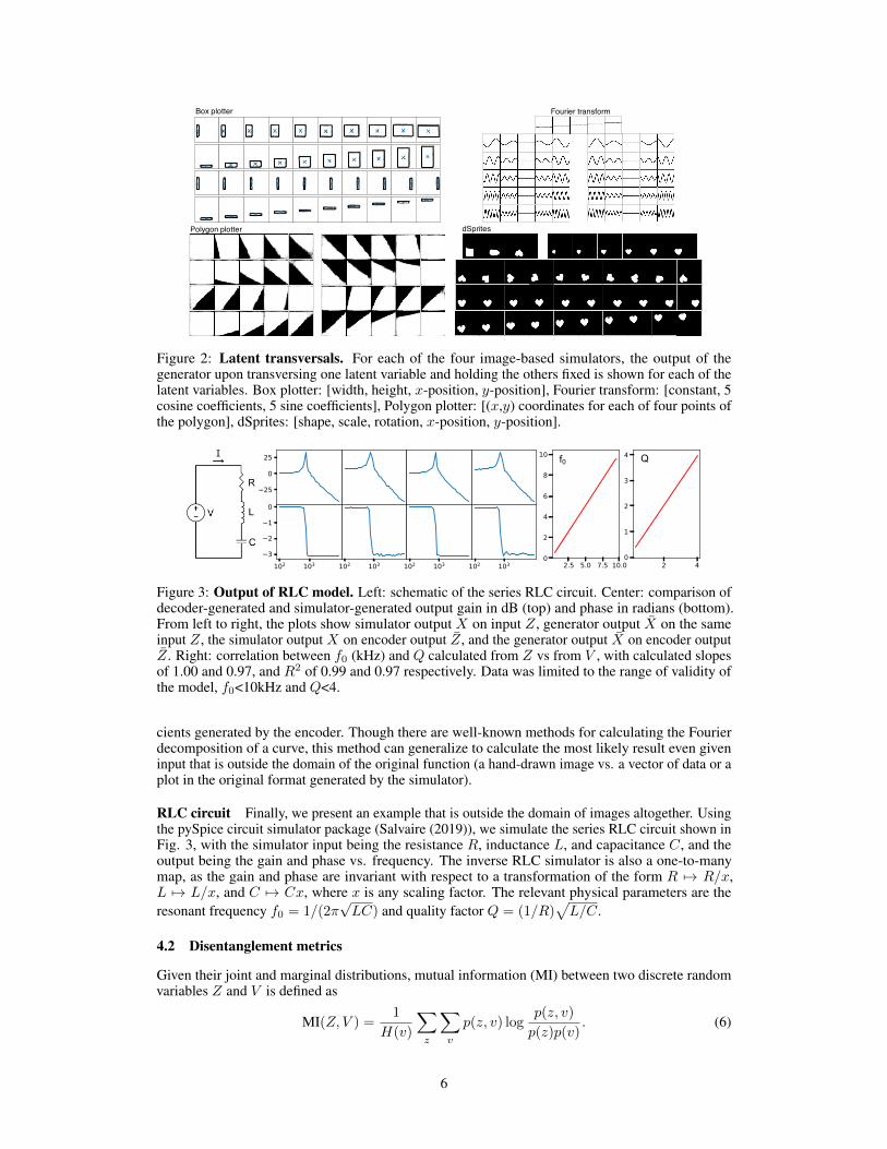
Figure 3: Output of RLC model. Left: schematic of the series RLC circuit. Center: comparison ofdecoder-generated and simulator-generated output gain in dB (top) and phase in radians (bottom).From left to right, the plots show simulator output X on input Z, generator output X̄ on the sameinput Z, the simulator output X on encoder output Z̄, and the generator output X̄ on encoder outputZ̄. Right: correlation between f0 (kHz) and Q calculated from Z vs from V , with calculated slopesof 1.00 and 0.97, and R2 of 0.99 and 0.97 respectively. Data was limited to the range of validity ofthe model, f0<10kHz and Q<4.
cients generated by the encoder. Though there are well-known methods for calculating the Fourierdecomposition of a curve, this method can generalize to calculate the most likely result even giveninput that is outside the domain of the original function (a hand-drawn image vs. a vector of data or aplot in the original format generated by the simulator).
RLC circuit Finally, we present an example that is outside the domain of images altogether. Usingthe pySpice circuit simulator package (Salvaire (2019)), we simulate the series RLC circuit shown inFig. 3, with the simulator input being the resistance R, inductance L, and capacitance C, and theoutput being the gain and phase vs. frequency. The inverse RLC simulator is also a one-to-manymap, as the gain and phase are invariant with respect to a transformation of the form R 7→ R/x,L 7→ L/x, and C 7→ Cx, where x is any scaling factor. The relevant physical parameters are theresonant frequency f0 = 1/(2π
√LC) and quality factor Q = (1/R)
√L/C.
4.2 Disentanglement metrics
Given their joint and marginal distributions, mutual information (MI) between two discrete randomvariables Z and V is defined as
MI(Z, V ) =1
H(v)
∑z
∑v
p(z, v) logp(z, v)
p(z)p(v). (6)
6
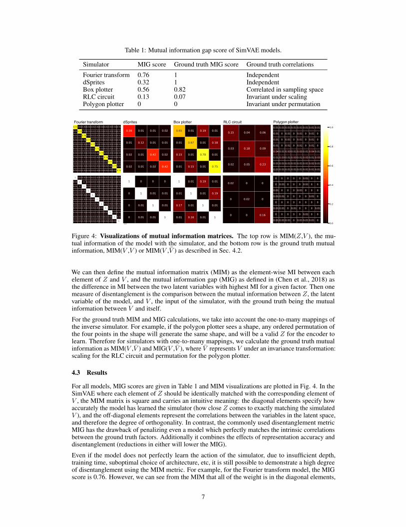
Table 1: Mutual information gap score of SimVAE models.
Simulator MIG score Ground truth MIG score Ground truth correlations
Fourier transform 0.76 1 IndependentdSprites 0.32 1 IndependentBox plotter 0.56 0.82 Correlated in sampling spaceRLC circuit 0.13 0.07 Invariant under scalingPolygon plotter 0 0 Invariant under permutation
Fourier transform Box plotterdSprites RLC circuit Polygon plotter
Figure 4: Visualizations of mutual information matrices. The top row is MIM(Z,V ), the mu-tual information of the model with the simulator, and the bottom row is the ground truth mutualinformation, MIM(V ,V ) or MIM(V ,V̄ ) as described in Sec. 4.2.
We can then define the mutual information matrix (MIM) as the element-wise MI between eachelement of Z and V , and the mutual information gap (MIG) as defined in (Chen et al., 2018) asthe difference in MI between the two latent variables with highest MI for a given factor. Then onemeasure of disentanglement is the comparison between the mutual information between Z, the latentvariable of the model, and V , the input of the simulator, with the ground truth being the mutualinformation between V and itself.
For the ground truth MIM and MIG calculations, we take into account the one-to-many mappings ofthe inverse simulator. For example, if the polygon plotter sees a shape, any ordered permutation ofthe four points in the shape will generate the same shape, and will be a valid Z for the encoder tolearn. Therefore for simulators with one-to-many mappings, we calculate the ground truth mutualinformation as MIM(V ,V̄ ) and MIG(V ,V̄ ), where V̄ represents V under an invariance transformation:scaling for the RLC circuit and permutation for the polygon plotter.
4.3 Results
For all models, MIG scores are given in Table 1 and MIM visualizations are plotted in Fig. 4. In theSimVAE where each element of Z should be identically matched with the corresponding element ofV , the MIM matrix is square and carries an intuitive meaning: the diagonal elements specify howaccurately the model has learned the simulator (how close Z comes to exactly matching the simulatedV ), and the off-diagonal elements represent the correlations between the variables in the latent space,and therefore the degree of orthogonality. In contrast, the commonly used disentanglement metricMIG has the drawback of penalizing even a model which perfectly matches the intrinsic correlationsbetween the ground truth factors. Additionally it combines the effects of representation accuracy anddisentanglement (reductions in either will lower the MIG).
Even if the model does not perfectly learn the action of the simulator, due to insufficient depth,training time, suboptimal choice of architecture, etc, it is still possible to demonstrate a high degreeof disentanglement using the MIM metric. For example, for the Fourier transform model, the MIGscore is 0.76. However, we can see from the MIM that all of the weight is in the diagonal elements,
7
and therefore in practice this is a fully disentangled representation. The missing mutual informationis from insufficient model strength to match the simulator, and not in any correlations between thelatent variables.
This similarly holds for the dSprites dataset - the latent variables are fully orthogonal, even thoughthe representation accuracy is not complete. As calculated in (Locatello et al., 2018), MIG scores fora selection of models on the dSprites dataset fall between a wide range of 0-0.4 depending on thechoice of hyperparameters. Our model gives a MIG score of 0.32 on the (scale, rotation, x-position,y-position) factors of dSprites (treating the shape factor as noise, as in (Chen et al., 2018)), whichfalls within this range. But as can be seen from the full MIM in Fig. 4, the latent variables are fullydisentangled, and the limit of mutual information is due to the quality of fit to the dataset rather thaninformation mixing between latent variables. A different neural network architecture could be usedto improve fit, or if a more accurate fit were prioritized over the matching of Z with V , the latentspace could be expanded with additional non-interpretable latent variables.
Note, however, that a lack of orthogonality also does not necessarily imply that the latent spaceis not interpretable. In the example of the 2D box plotter, the simulator was formulated with aninherent correlation between the variables of V : that the box must always remain fully within thespecified plotting range, and therefore the width and height are correlated with the x and y coordinatesrespectively. Given this simple correlation built into the system, we can see that even in correlatingV with itself - as would be the case when Z perfectly learns V - there remains mutual informationbetween the latent variables. By penalizing this correlation, as would be imposed for β-VAE forexample, the model would be required to deviate from the natural variables specified in the problemand would likely have a reduced representation accuracy.
In cases such as the RLC circuit and polygon plotter, where the inverse simulator has a one-to-manymapping, both the MIM and MIG are uninformative. Though the latent variables Z themselves aremeaningful, as demonstrated by the quality of representation and transversals, they don’t have a fixedrelationship with the V values from the simulator. Hence, the mutual information drives towards zeroas the space for scaling and permutation expands. We raise a task for future work to identify a metricto quantify disentanglement and interpretability that can distinguish between representation accuracyand disentanglement, and which is effective in the case of many-to-one and one-to-many mappings.
5 Discussion
In this paper we present SimVAE, a new approach for simulator-based training of variational au-toencoders. Our approach is general and can hypothetically work with any simulator (assuming thatthe backbone network is expressive enough). We demonstrated its breadth by applying it to severaldomains, some of which are very different from visual scene understanding which was the focus ofprevious work on learning disentangled representations. A key aspect of our approach is to separatethe training to two stages: a supervised stage where a generative model approximating the simulatoris learned, and an unsupervised stage where an inference model approximating the inverse of thesimulator is learned. It is interesting to note that typically generative models are associated withunsupervised learning while inference (discriminative) models are associated with supervision. Herewe show that the opposite can yield powerful models.
When considering the world as a complex simulator, our decoupled semi-supervised approachsuggests interesting directions to explore in the context of machines vs. humans learning. A SimVAEmodel can be initialized in an unsupervised manner using a VAE or GAN approach (in our experimentswe did not need this stage), followed by a supervised stage of training the generator and then anunsupervised one of training the encoder. Moving forward, both models can be continuously traineddepending on the data that the system receives: when the observed data is coupled with labels(namely, values of latent variables) the supervised generator training kicks in, and when it is not, theunsupervised encoder training kicks in. When babies sense the world, they similarly receive bothlabeled and unlabaled data: most of the time they observe the world without supervision, but everynow and then someone points to an object saying ’this is a red ball’. It is therefore intriguing toexplore whether alternating between supervised and unsupervised learning of approximate simulationand its inverse respectively, are at work in human learning.
An interesting direction for future research is to explore compositionality. As opposed to unsupervisedapproaches such as InfoGAN or β-VAE, our approach can learn exactly the latent variables of interest
8
for downstream applications. For example consider the problem of learning to multiply hand writtennumbers. One can first learn models that generate and recognize hand written digits by approximatinga digits graphics engine. Then given a multiplication simulator, one can learn models that multiplyand factor hand written numbers up to 81 (9X9) and use the digits generator to generate the ’handwritten’ result. In order to learn in general how to multiply multi-digit numbers, causality is key (Lakeet al., 2017). Namely, fine grained simulators of the components of the multiplication algorithm willhave to be learned (note that this is how children learn to do it at school). This idea, with a differentlearning technique, was explored in the context of hand written characters (Lake et al., 2015). Infuture work we plan to explore compositionality and causality as well as applications of our approachto more complex simulators such as photo-realistic graphics engines.
ReferencesChen, Tian Qi, Li, Xuechen, Grosse, Roger B., and Duvenaud, David K. Isolating sources of
disentanglement in variational autoencoders. CoRR, abs/1802.04942, 2018. URL http://arxiv.org/abs/1802.04942.
Chen, Xi, Duan, Yan, Houthooft, Rein, Schulman, John, Sutskever, Ilya, and Abbeel, Pieter. InfoGAN:Interpretable representation learning by information maximizing generative adversarial nets. InAdvances in neural information processing systems, pp. 2172–2180, 2016.
Goodfellow, Ian, Pouget-Abadie, Jean, Mirza, Mehdi, Xu, Bing, Warde-Farley, David, Ozair, Sherjil,Courville, Aaron, and Bengio, Yoshua. Generative adversarial nets. In Advances in neuralinformation processing systems, pp. 2672–2680, 2014.
Gretton, Arthur, Borgwardt, Karsten M, Rasch, Malte J, Schölkopf, Bernhard, and Smola, Alexander.A kernel two-sample test. Journal of Machine Learning Research, 13(Mar):723–773, 2012.
Higgins, Irina, Matthey, Loic, Pal, Arka, Burgess, Christopher, Glorot, Xavier, Botvinick, Matthew,Mohamed, Shakir, and Lerchner, Alexander. beta-VAE: Learning basic visual concepts with aconstrained variational framework. In International Conference on Learning Representations,volume 3, 2017.
Hunter, J. D. Matplotlib: A 2D graphics environment. Computing in Science & Engineering, 9(3):90–95, 2007. doi: 10.1109/MCSE.2007.55.
Jiajun Wu, Joshua B. Tenenbaum, Pushmeet Kohli. Neural scene de-rendering. In Computer Visionand Pattern Recognition (CVPR), pp. 7035–7043, 2017a.
Jiajun Wu, Erika Lu, Pushmeet Kohli Bill Freeman Josh Tenenbaum. Learning to see physicsvia visual de-animation. In Conference on Neural Information Processing Systems (NIPS), pp.152–163, 2017b.
Kingma, Diederik P and Ba, Jimmy. Adam: A method for stochastic optimization. In InternationalConference on Learning Representations (ICLR), 2015.
Kingma, Diederik P and Welling, Max. Auto-encoding variational bayes. In International Conferenceon Learning Representations (ICLR), 2014.
Kulkarni, Tejas D, Whitney, William F, Kohli, Pushmeet, and Tenenbaum, Josh. Deep convolutionalinverse graphics network. In Advances in neural information processing systems, pp. 2539–2547,2015.
Kullback, Solomon and Leibler, Richard A. On information and sufficiency. The annals of mathemat-ical statistics, 22(1):79–86, 1951.
Lake, B. M., Salakhutdinov, R., and Tenenbaum, J. B. Human-level concept learning throughprobabilistic program induction. Science, 350(6266):1332–1388, 2015.
Lake, Brenden M., Ullman, Tomer D., Tenenbaum, Joshua B., and Gershman, Samuel J. Buildingmachines that learn and think like people. Behavioral and Brain Sciences, 40, 2017.
9
Locatello, Francesco, Bauer, Stefan, Lucic, Mario, Gelly, Sylvain, Schölkopf, Bernhard, and Bachem,Olivier. Challenging common assumptions in the unsupervised learning of disentangled represen-tations. CoRR, abs/1811.12359, 2018. URL http://arxiv.org/abs/1811.12359.
N Siddharth, T. B. Paige, J.W. Meent A. Desmaison N. Goodman P. Kohli F. Wood and Torr, P.Learning disentangled representations with semi-supervised deep generative models. In Conferenceon Neural Information Processing Systems (NIPS), pp. 5927–5937, 2017.
Radford, Alec, Metz, Luke, and Chintala, Soumith. Unsupervised representation learning withdeep convolutional generative adversarial networks. In International Conference on LearningRepresentations (ICLR), 2016.
Salvaire, Fabrice. Pyspice. https://pyspice.fabrice-salvaire.fr, 2019.
10