Simultaneous Robust Design and Tolerancingof Compressor Blades

Eric Dow

Aerospace Computational Design LaboratoryDepartment of Aeronautics and Astronautics

Massachusetts Institute of Technology

GTL SeminarOctober 1, 2013

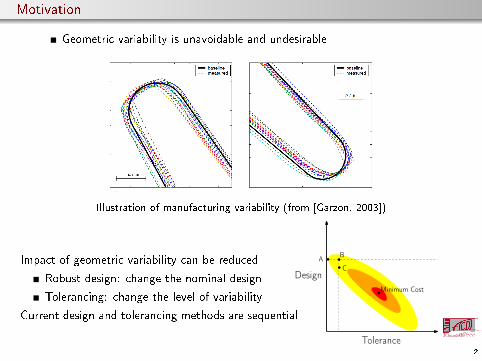
Motivation

Geometric variability is unavoidable and undesirable

Illustration of manufacturing variability (from [Garzon, 2003])

Impact of geometric variability can be reduced

Robust design: change the nominal design

Tolerancing: change the level of variability

Current design and tolerancing methods are sequential

Design

Tolerance

Minimum Cost

AB

C

2

Performance Impacts of Geometric Variability

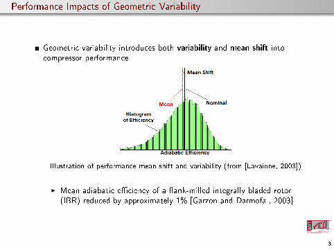
Geometric variability introduces both variability and mean shift intocompressor performance

Illustration of performance mean shift and variability (from [Lavainne, 2003])

I Mean adiabatic eciency of a ank-milled integrally bladed rotor(IBR) reduced by approximately 1% [Garzon and Darmofal, 2003]

3

Research Objectives

1 Develop a framework for simultaneous robust design and toleranceoptimization that incorporates manufacturing and operating costs

2 Develop an approach for probabilistic sensitivity analysis of performancewith respect to the level of variability

3 Demonstrate framework eectiveness for design and tolerancing ofturbomachinery compressor blades

4

The Pitfalls of Single-point Optimization

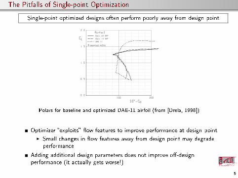
Single-point optimized designs often perform poorly away from design point

Polars for baseline and optimized DAE-11 airfoil (from [Drela, 1998])

Optimizer exploits ow features to improve performance at design point

I Small changes in ow features away from design point may degradeperformance

Adding additional design parameters does not improve o-designperformance (it actually gets worse!)

5

Robust Design Optimization

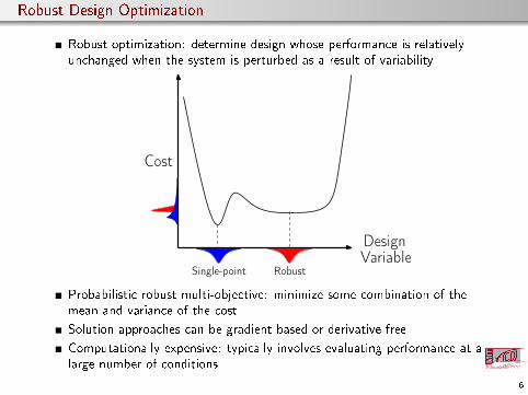
Robust optimization: determine design whose performance is relativelyunchanged when the system is perturbed as a result of variability

Design

Cost

Single-point RobustVariable

Probabilistic robust multi-objective: minimize some combination of themean and variance of the cost

Solution approaches can be gradient-based or derivative-free

Computationally expensive: typically involves evaluating performance at alarge number of conditions

6

Modelling Variability: Random Fields

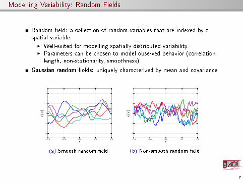
Random eld: a collection of random variables that are indexed by aspatial variable

I Well-suited for modelling spatially distributed variabilityI Parameters can be chosen to model observed behavior (correlation

length, non-stationarity, smoothness)

Gaussian random elds: uniquely characterized by mean and covariance

−1.0 −0.5 0.0 0.5 1.0s

−4

−2

0

2

4

e(s)

(a) Smooth random eld

−1.0 −0.5 0.0 0.5 1.0s

−4

−2

0

2

4

e(s)

(b) Non-smooth random eld

7

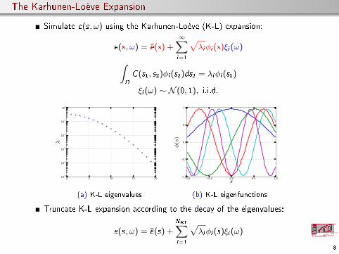
The Karhunen-Loève Expansion

Simulate e(s, ω) using the Karhunen-Loève (K-L) expansion:

e(s, ω) = e(s) +∞∑i=1

√λiφi (s)ξi (ω)∫

D

C(s1, s2)φi (s2)ds2 = λiφi (s1)

ξi (ω) ∼ N (0, 1), i.i.d.

0 5 10 15 2010-5

10-4

10-3

10-2

10-1

100

λ

(a) K-L eigenvalues

−1.0 −0.5 0.0 0.5 1.0s

−1.0

−0.5

0.0

0.5

1.0

φ(s

)

(b) K-L eigenfunctions

Truncate K-L expansion according to the decay of the eigenvalues:

e(s, ω) = e(s) +

NKL∑i=1

√λiφi (s)ξi (ω)

8

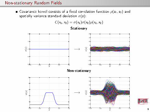
Non-stationary Random Fields

Covariance kernel consists of a xed correlation function ρ(s1, s2) andspatially variance standard deviation σ(s):

C(s1, s2) = σ(s1)σ(s2)ρ(s1, s2)

Stationary

−1.0 −0.5 0.0 0.5 1.0s

0.0

0.5

1.0

1.5

2.0

σ(s

) −→

−1.0 −0.5 0.0 0.5 1.0s

−20

−15

−10

−5

0

5

10

15

20

e(s)

Non-stationary

−1.0 −0.5 0.0 0.5 1.0s

0

2

4

6

8

10

σ(s

) −→

−1.0 −0.5 0.0 0.5 1.0s

−20

−15

−10

−5

0

5

10

15

20

e(s)

9

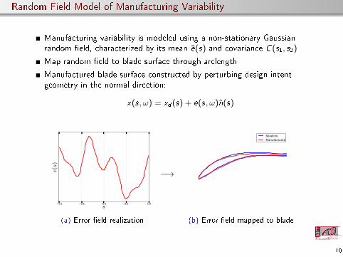
Random Field Model of Manufacturing Variability

Manufacturing variability is modeled using a non-stationary Gaussianrandom eld, characterized by its mean e(s) and covariance C(s1, s2)

Map random eld to blade surface through arclength

Manufactured blade surface constructed by perturbing design intentgeometry in the normal direction:

x(s, ω) = xd (s) + e(s, ω)n(s)

−1.0 −0.5 0.0 0.5 1.0s

e(s)

(a) Error eld realization

−→

BaselineManufactured

(b) Error eld mapped to blade

10

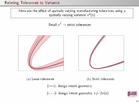
Relating Tolerances to Variance

Simulate the eect of spatially varying manufacturing tolerances using aspatially varying variance σ2(s)

Small σ2 → strict tolerances

(a) Loose tolerances (b) Strict tolerances

(): design intent geometry

(- - -): design intent geometry +/- 2σ(s)

11

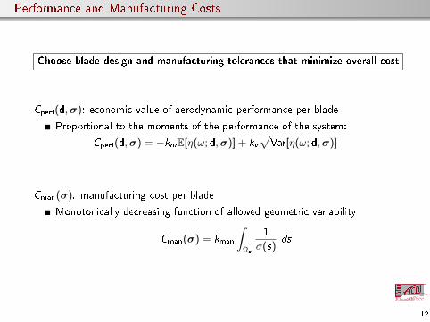
Performance and Manufacturing Costs

Choose blade design and manufacturing tolerances that minimize overall cost

Cperf(d,σ): economic value of aerodynamic performance per blade

Proportional to the moments of the performance of the system:

Cperf(d,σ) = −kmE[η(ω; d,σ)] + kv√Var[η(ω; d,σ)]

Cman(σ): manufacturing cost per blade

Monotonically decreasing function of allowed geometric variability

Cman(σ) = kman

∫Ωs

1

σ(s)ds

12

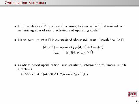
Optimization Statement

Optimal design (d∗) and manufacturing tolerances (σ∗) determined byminimizing sum of manufacturing and operating costs

Mean pressure ratio Π is constrained above minimum allowable value Π

(d∗,σ∗) = argmin Cperf(d,σ) + Cman(σ)

s.t. E[Π(d,σ, ω)] ≥ Π

Gradient-based optimization: use sensitivity information to choose searchdirections

I Sequential Quadratic Programming (SQP)

13

Model Problem of Interest

In the absence of variability, nominal design variables d determines thePDE solution u

Random eld e(s, ω) introduces random noise to the solution

System performance characterized by the moments of functionals F (u) ofthe solution, e.g. E[F ] and Var[F (u)]

Random Field

e(s, ω; σ)

Standard

Deviation σ

Correlation

Structure ρ

PDE Solution

u(y ; d)

PDE Solution

u(y, ω; d,σ)

Nominal

Design

Variables d

Performance

Moments

E[F (u(y, ω; d,σ))]

14

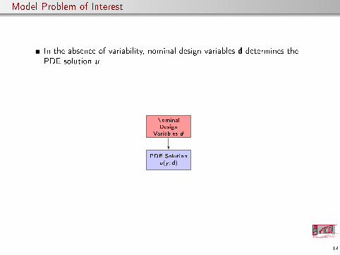
Model Problem of Interest

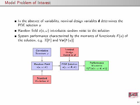
In the absence of variability, nominal design variables d determines thePDE solution u

Random eld e(s, ω) introduces random noise to the solution

System performance characterized by the moments of functionals F (u) ofthe solution, e.g. E[F ] and Var[F (u)]

Random Field

e(s, ω; σ)

Standard

Deviation σ

Correlation

Structure ρ

PDE Solution

u(y ; d)PDE Solution

u(y, ω; d,σ)

Nominal

Design

Variables d

Performance

Moments

E[F (u(y, ω; d,σ))]

14

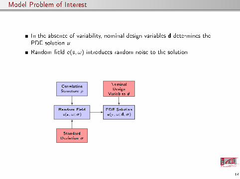
Model Problem of Interest

In the absence of variability, nominal design variables d determines thePDE solution u

Random eld e(s, ω) introduces random noise to the solution

System performance characterized by the moments of functionals F (u) ofthe solution, e.g. E[F ] and Var[F (u)]

Random Field

e(s, ω; σ)

Standard

Deviation σ

Correlation

Structure ρ

PDE Solution

u(y ; d)PDE Solution

u(y, ω; d,σ)

Nominal

Design

Variables d

Performance

Moments

E[F (u(y, ω; d,σ))]

14

Monte Carlo Method

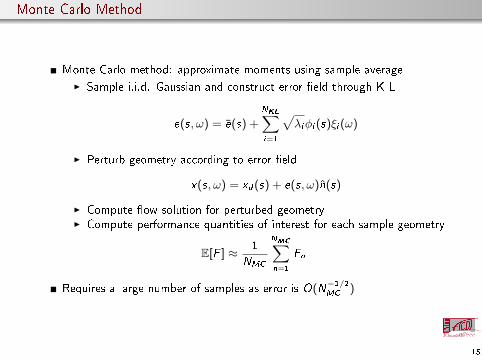
Monte Carlo method: approximate moments using sample average

I Sample i.i.d. Gaussian and construct error eld through K-L

e(s, ω) = e(s) +

NKL∑i=1

√λiφi (s)ξi (ω)

I Perturb geometry according to error eld

x(s, ω) = xd (s) + e(s, ω)n(s)

I Compute ow solution for perturbed geometryI Compute performance quantities of interest for each sample geometry

E[F ] ≈ 1

NMC

NMC∑n=1

Fn

Requires a large number of samples as error is O(N−1/2MC )

15

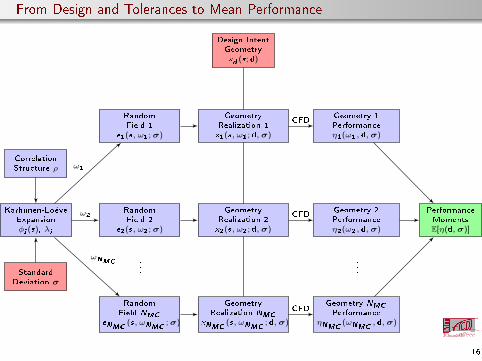
From Design and Tolerances to Mean Performance

Karhunen-Loève

Expansion

φi (s), λi

Standard

Deviation σ

Correlation

Structure ρ

Random

Field 2

e2(s, ω2; σ)

Random

Field 1

e1(s, ω1; σ)

.

.

.

Random

Field NMCeNMC

(s, ωNMC; σ)

Geometry

Realization NMCxNMC

(s, ωNMC; d,σ)

Design Intent

Geometry

xd

(s; d)

Geometry

Realization 2

x2(s, ω2; d,σ)

Geometry

Realization 1

x1(s, ω1; d,σ)

Geometry 1

Performance

η1(ω1, d,σ)

Geometry 2

Performance

η2(ω2, d,σ)

Geometry NMCPerformance

ηNMC(ωNMC

, d,σ)

.

.

.

Performance

Moments

E[η(d,σ)]

ω1

ω2

ωNMC

CFD

CFD

CFD

16

Sensitivity Analysis Overview

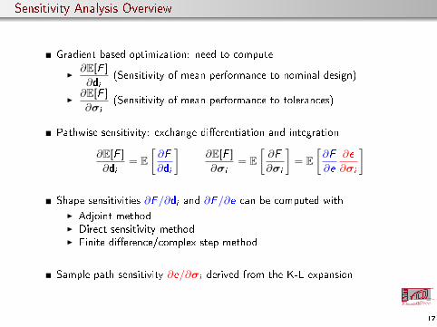
Gradient based optimization: need to compute

I∂E[F ]

∂di(Sensitivity of mean performance to nominal design)

I∂E[F ]

∂σi

(Sensitivity of mean performance to tolerances)

Pathwise sensitivity: exchange dierentiation and integration

∂E[F ]

∂di= E

[∂F

∂di

]∂E[F ]

∂σi

= E[∂F

∂σi

]= E

[∂F

∂e

∂e

∂σi

]

Shape sensitivities ∂F/∂di and ∂F/∂e can be computed with

I Adjoint methodI Direct sensitivity methodI Finite dierence/complex step method

Sample path sensitivity ∂e/∂σi derived from the K-L expansion

17

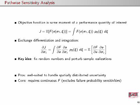
Pathwise Sensitivity Analysis

Objective function is some moment of a performance quantity of interest

J = E[F (e(σi , ξ))] =

∫F (e(σi , ξ)) pΞ(ξ) dξ

Exchange dierentiation and integration:

∂J

∂σi

=

∫∂F

∂e

∂e

∂σi

pΞ(ξ) dξ = E[∂F

∂e

∂e

∂σi

]Key idea: x random numbers and perturb sample realizations

Pros: well-suited to handle spatially distributed uncertainty

Cons: requires continuous F (excludes failure probability sensitivities)

18

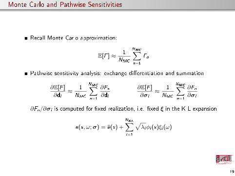
Monte Carlo and Pathwise Sensitivities

Recall Monte Carlo approximation:

E[F ] ≈ 1

NMC

NMC∑n=1

Fn

Pathwise sensitivity analysis: exchange dierentiation and summation

∂E[F ]

∂di≈ 1

NMC

NMC∑n=1

∂Fn∂di

∂E[F ]

∂σi

≈ 1

NMC

NMC∑n=1

∂Fn∂σi

∂Fn/∂σi is computed for xed realization, i.e. xed ξ in the K-L expansion

e(s, ω;σ) = e(s) +

NKL∑i=1

√λiφi (s)ξi (ω)

19

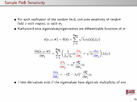
Sample Path Sensitivity

For each realization of the random eld, compute sensitivity of randomeld e with respect to each σj

Karhunen-Loève eigenvalues/eigenvectors are dierentiable functions of σ:

e(s, ω;σ) = e(s) +

NKL∑i=1

√λiφi (s)ξi (ω)

∂e(s, ω;σ)

∂σj

=

NKL∑i=1

(1

2√λiφi∂λi∂σj

+√λi∂φi∂σj

)ξi (ω)

∂λi∂σj

= φTi∂C

∂σj

φi

∂φi∂σj

= −(C− λi I )+ ∂C

∂σj

φi

These derivatives exist if the eigenvalues have algebraic multiplicity of one

20

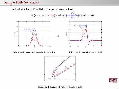
Sample Path Sensitivity

Holding xed ξ in K-L expansion ensures that

δσ(s) small⇒ e(s) and e(s) +δe

δσδσ(s) are close

1.0 0.5 0.0 0.5 1.0

s0.000

0.002

0.004

0.006

0.008

0.010

σ(s

)

σ(s)

σ(s) + δσ(s)

Initial and perturbed standard deviation

⇒

1.0 0.5 0.0 0.5 1.0

s0.4

0.2

0.0

0.2

0.4

0.6

0.8

1.0

1.2

1.4

e(s

)

1e 2

e(s)

e(s) + ∂e∂σδσ(s)

Initial and perturbed error eld

xd

xd + e

xd + e + δe

Initial and perturbed manufactured blade 21

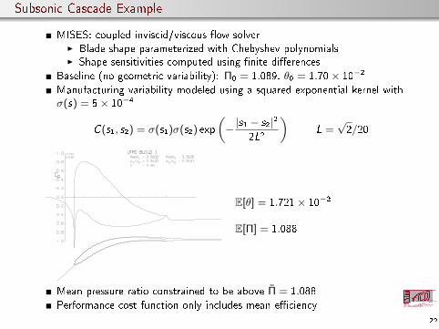
Subsonic Cascade Example

MISES: coupled inviscid/viscous ow solverI Blade shape parameterized with Chebyshev polynomialsI Shape sensitivities computed using nite dierences

Baseline (no geometric variability): Π0 = 1.089, θ0 = 1.70× 10−2

Manufacturing variability modeled using a squared exponential kernel withσ(s) = 5× 10−4

C(s1, s2) = σ(s1)σ(s2) exp

(−|s1 − s2|2

2L2

)L =√2/20

E[θ] = 1.721× 10−2

E[Π] = 1.088

Mean pressure ratio constrained to be above Π = 1.088

Performance cost function only includes mean eciency

22

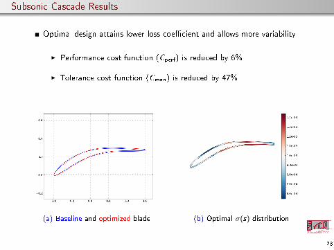
Subsonic Cascade Results

Optimal design attains lower loss coecient and allows more variability

I Performance cost function (Cperf) is reduced by 6%

I Tolerance cost function (Cman) is reduced by 47%

(a) Baseline and optimized blade (b) Optimal σ(s) distribution

23

Summary and Future Work

New framework for simultaneous robust design and tolerancing

I Manufacturing and operating costs incorporated into optimizationI Create a feedback loop between designers and manufacturers

Novel probabilistic sensitivity analysis of performance to level of variability

Optimal blade performs better and is cheaper to manufacture

Future Work

More accurate/ecient shape sensitivities: direct sensitivity method

Transonic compressor optimization

Investigate solution quality

24

Questions?

25

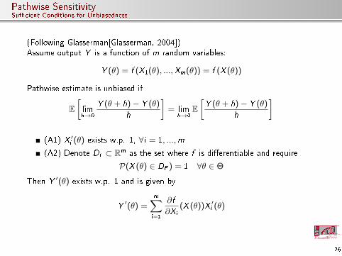
Pathwise SensitivitySucient Conditions for Unbiasedness

(Following Glasserman[Glasserman, 2004])Assume output Y is a function of m random variables:

Y (θ) = f (X1(θ), ...,Xm(θ)) = f (X (θ))

Pathwise estimate is unbiased if

E[limh→0

Y (θ + h)− Y (θ)

h

]= lim

h→0E[Y (θ + h)− Y (θ)

h

]

(A1) X ′i (θ) exists w.p. 1, ∀i = 1, ...,m

(A2) Denote Df ⊂ Rm as the set where f is dierentiable and require

P(X (θ) ∈ DF ) = 1 ∀θ ∈ Θ

Then Y ′(θ) exists w.p. 1 and is given by

Y′(θ) =

m∑i=1

∂f

∂Xi

(X (θ))X ′i (θ)

26

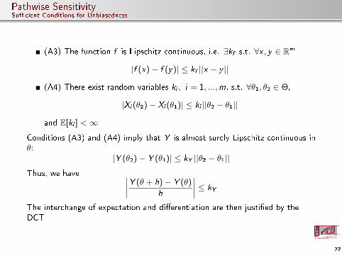
Pathwise SensitivitySucient Conditions for Unbiasedness

(A3) The function f is Lipschitz continuous, i.e. ∃kf s.t. ∀x , y ∈ Rm

|f (x)− f (y)| ≤ kf ||x − y ||

(A4) There exist random variables ki , i = 1, ...,m, s.t. ∀θ1, θ2 ∈ Θ,

|Xi (θ2)− Xi (θ1)| ≤ ki ||θ2 − θ1||

and E[ki ] <∞

Conditions (A3) and (A4) imply that Y is almost surely Lipschitz continuous inθ:

|Y (θ2)− Y (θ1)| ≤ kY ||θ2 − θ1||

Thus, we have ∣∣∣∣Y (θ + h)− Y (θ)

h

∣∣∣∣ ≤ kY

The interchange of expectation and dierentiation are then justied by theDCT

27

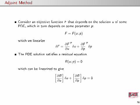
Adjoint Method

Consider an objective function F that depends on the solution u of somePDE, which in turn depends on some parameter p:

F = F (u; p)

which we linearize

δF =∂F

∂u

T

δu +∂F

∂p

T

δp

The PDE solution satises a residual equation

R(u; p) = 0

which can be linearized to give[∂R

∂u

]δu +

[∂R

∂p

]δp = 0

28

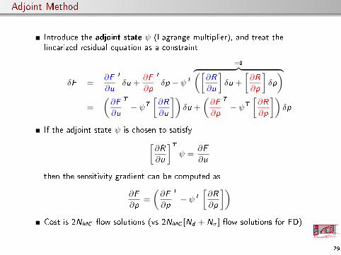
Adjoint Method

Introduce the adjoint state ψ (Lagrange multiplier), and treat thelinearized residual equation as a constraint

δF =∂F

∂u

T

δu +∂F

∂p

T

δp − ψT

=0︷ ︸︸ ︷([∂R

∂u

]δu +

[∂R

∂p

]δp

)=

(∂F

∂u

T

− ψT

[∂R

∂u

])δu +

(∂F

∂p

T

− ψT

[∂R

∂p

])δp

If the adjoint state ψ is chosen to satisfy[∂R

∂u

]Tψ =

∂F

∂u

then the sensitivity gradient can be computed as

∂F

∂p=

(∂F

∂p

T

− ψT

[∂R

∂p

])Cost is 2NMC ow solutions (vs 2NMC [Nd + Nσ] ow solutions for FD)

29

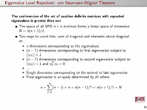
Eigenvalue Level Repulsion: von Neumann-Wigner Theorem

The codimension of the set of positive denite matrices with repeated

eigenvalues is greater than one

The space of all SPD n × n matrices forms a linear space of dimensionN = n(n + 1)/2.

Two ways to count this: sum of diagonal and elements above diagonal,or...

I n dimensions corresponding to the eigenvaluesI (n − 1) dimensions corresponding to rst eigenvector subject to||φ1|| = 1

I (n − 2) dimensions corresponding to second eigenvector subject to||φ2|| = 1 and φT1 φ2 = 0

I ...I Single dimension corresponding to the second to last eigenvectorI Final eigenvector is uniquely determined by all others

n +n∑i=1

(n − i) = n + n(n − 1)/2 = n(n + 1)/2 = N

30

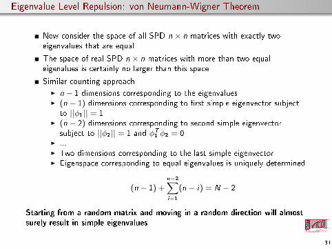
Eigenvalue Level Repulsion: von Neumann-Wigner Theorem

Now consider the space of all SPD n × n matrices with exactly twoeigenvalues that are equal

The space of real SPD n × n matrices with more than two equaleigenalues is certainly no larger than this space

Similar counting approach

I n − 1 dimensions corresponding to the eigenvaluesI (n − 1) dimensions corresponding to rst simple eigenvector subject

to ||φ1|| = 1I (n − 2) dimensions corresponding to second simple eigenvector

subject to ||φ2|| = 1 and φT1 φ2 = 0I ...I Two dimensions corresponding to the last simple eigenvectorI Eigenspace corresponding to equal eigenvalues is uniquely determined

(n − 1) +n−2∑i=1

(n − i) = N − 2

Starting from a random matrix and moving in a random direction will almost

surely result in simple eigenvalues

31

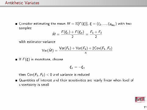
Antithetic Variates

Consider estimating the mean M = E[F (ξ)], ξ = (ξ1, ..., ξNKL) with twosamples:

M =F (ξ1) + F (ξ2)

2=

F1 + F2

2

with estimator variance

Var(M) =Var(F1) + Var(F2) + 2Cov(F1,F2)

4

If F (ξ) is monotone, choose

ξ1 = −ξ2

then Cov(F1,F2) < 0 and variance is reduced

Quantities of interest and their sensitivities are nearly linear when level ofuncertainty is small

32

References I

[Drela, 1998] Drela, M. (1998).

Frontiers of Computational Fluid Dynamics 1998, chapter 19, Pros and cons of airfoiloptimization, pages 363380.

World Scientic Publishing.

[Garzon, 2003] Garzon, V. E. (2003).

Probabilistic Aerothermal Design of Compressor Airfoils.

PhD dissertation, Massachusetts Institute of Technology, Department of Aeronautics andAstronautics.

[Garzon and Darmofal, 2003] Garzon, V. E. and Darmofal, D. (2003).

Impact of geometric variability on axial compressor performance.

Journal of Turbomachinery, 125(4):692703.

[Glasserman, 2004] Glasserman, P. (2004).

Monte Carlo Methods in Financial Engineering, chapter 7, Estimating Sensitivities, pages386401.

Springer Verlag, New York.

[Lavainne, 2003] Lavainne, J. (2003).

Sensitivity of a Compressor Repeating-Stage to Geometry Variation.

Master's dissertation, Massachusetts Institute of Technology, Department of Aeronauticsand Astronautics.

33