Embed Size (px)
Citation preview

Simultaneous Estimation of Microphysical Parameters and Atmospheric State with Simulated Radar Data and Ensemble Square-root Kalman Filter. Part I: Sensitivity Analysis and Parameter Identifiability
Mingjing Tong and Ming Xue
Center for Analysis and Prediction of Storms and School of Meteorology University of Oklahoma, Norman OK 73072
June, 2006 Submitted to Monthly Weather Review
Revised May and August 2007
Corresponding author address:
Ming Xue Center for Analysis and Prediction of Storms,
National Weather Center, Suite 2500, 120 David L. Boren Blvd, Norman, OK 73072

Abstract
The possibility of estimating fundamental parameters common in single-moment ice
microphysics schemes using radar observations is investigated, for a model-simulated supercell
storm, by examining parameter sensitivity and identifiability. These parameters include the
intercept parameters for rain, snow and hail/graupel, and the bulk densities of snow and
hail/graupel. These parameters are closely involved in the definition of drop/particle size
distributions of microphysical species but often assume highly uncertain specified values.
The sensitivity of model forecast within data assimilation cycles to the parameter values,
and the issue of solution uniqueness of the estimation problem are examined. The ensemble
square-root filter (EnSRF) is employed for model state estimation. Sensitivity experiments show
that the errors in the microphysical parameters have a larger impact on model microphysical
fields than on wind fields; radar reflectivity observations are therefore preferred over those of
radial velocity for microphysical parameter estimation. The model response time to errors in
individual parameters are also investigated. The results suggest that radar data should be used at
about 5 minute intervals for parameter estimation. The response functions calculated from
ensemble mean forecast for all five individual parameters show concave shapes, with unique
minima occurring at or very close to the true values; therefore true values of these parameters
can be retrieved at least in those cases where only one parameter contains error.
The identifiability of multiple parameters together is evaluated from their correlations
with forecast reflectivity. Significant levels of correlation are found that can be interpreted
physically. As the number of uncertain parameters increases, both the level and the area coverage
of significant correlations decrease, implying increased difficulties with multiple-parameter
estimation. The details of the estimation procedure and the results of a complete set of estimation
experiments will be presented in Part II of this paper.

1
1. Introduction
The accuracy of numerical weather prediction (NWP) depends very much on the
accuracy of the initial state estimation and the accuracy of the prediction model. Various
advanced data assimilation techniques have been developed in the recent decades that improve
the estimation of model initial conditions. Among these methods are the four-dimensional
variational assimilation (4DVAR) (Le Dimet and Talagrand 1986; Courtier and Talagrand 1987)
and the ensemble-based assimilation methods (Evensen 1994; Evensen and Leeuwen 1996;
Burgers et al. 1998; Houtekamer and Mitchell 1998; Anderson 2001; Bishop et al. 2001;
Whitaker and Hamill 2002b; Evensen 2003; Tippett et al. 2003), which have the advantage of
closely involving a numerical model in the data assimilation process. However, errors in the
model can directly affect the effectiveness of these data assimilation methods.
For convective-scale NWP, explicit microphysics schemes are used to predict the
evolution of clouds and precipitation. Most microphysics schemes use the 'bulk' approach of
parameterization, in which the particle or drop size distributions (DSDs) are parameterized in
functional forms. Often, significant uncertainties exist with the treatment of the microphysical
processes and the microphysical parameters. Previous sensitivity studies (e.g. McCumber et al.
1991; Ferrier et al. 1995; Gilmore et al. 2004; van den Heever and Cotton 2004) demonstrate that
the structure and evolution of simulated convective systems are very sensitive to microphysical
parameterizations. Variations in microphysical parameters, such as collection efficiencies, DSD
parameters and particle densities, have profound effects upon the characteristics of precipitation
systems and their associated dynamical processes.
Because of many assumptions involved, the microphysical parameterization can be an
important source of model error for convective-scale data assimilation and prediction. Parameter
estimation is a common approach to dealing with model error associated with uncertain

2
parameters. The inverse problem of parameter estimation concerns with the optimal
determination of the parameter by observing the dependent variable(s) collected in the spatial
and time domains (Yeh 1986). Various methods have been used for parameter estimation, among
which variational parameter estimation with an adjoint model is popular in the literature of
meteorology and oceanography (Navon 1998). The ensemble Kalman filter method (hereafter
EnKF) has recently been tested successfully for the atmospheric state estimation at the
convective scale with simulated (Snyder and Zhang 2003; Zhang et al. 2004; Tong and Xue 2005;
Xue et al. 2006) and real (Dowell et al. 2004; Tong 2006) radar data. The results with simulated
data, under the perfect model assumption, have been excellent, while the quality of state
estimation with real data, when model error inevitably exists, is generally not as good. More
recently, Aksoy et al. (2006) used EnKF for the simultaneous estimation of state variables and up
to six parameters in a relatively simple two-dimensional sea-breeze model with encouraging
success.
In this study, we set out to investigate the ability of the EnKF in correcting the errors in
some of the fundamental parameters in model microphysics, where complex process interactions
and high nonlinearities usually exist. In the framework of EnKF, parameter estimation is realized
by treating the uncertain parameters as independent model variables and using the covariance
information sampled from the ensemble to estimate the parameters given available observations
(Anderson 2001). This is often referred to as state vector augmentation technique where the
model parameters are considered part of the augmented state vector. Model state variables and
parameters are estimated simultaneously, through continuous assimilation cycles. The latest
estimation will be used for subsequent forecast.
The well-posedness as well as parameter identifiability are the main issues that are
directly related to the possibility of successful parameter estimation, no matter what technique is

3
used. The concept of identifiability addresses the question of whether it is at all possible to
obtain unique solutions of the inverse problem for unknown parameters of interest in a model
from data collected in the spatial and time domains (Navon 1998). The inverse problem for
parameter estimation is often ill-posed (Chavent 1974; Yakowitz and Duckstein 1980). As was
reviewed by Yeh (1986), the ill-posedness is generally characterized by the non-uniqueness and
instability of the identified parameters. In the case of non-uniqueness, the estimated value often
depends on its initial guess and is not guaranteed to be close to the “true” value. The instability
of the inverse solution stems from the fact that small errors in the observations will cause serious
errors in the identified parameters. Yakowitz and Duckstein (1980) demonstrated that a small
sensitivity of the model output in terms of observations to the change of unknown parameters
(parameters to be estimated) implies identification instability. The problem is that a larger
difference in the parameter may be manifested by only very small changes in the model output of
observed quantities, which may be smaller than anticipated measurement error.
As the first part of this study, we investigate the possibility of retrieving some
microphysical parameters with the EnKF method through a detailed sensitivity analysis. The
issue of parameter identifiability will be addressed. The results will guide our design of the
parameter estimation experiments and also help us understand the estimation results. Such an
investigation is necessary because we are dealing with a complex, highly nonlinear system, and
the feasibility of estimating DSD-related parameters using a full model and radar observations
has not been studied before. The microphysical parameters to be estimated are the intercept
parameters of rain, snow, and hail/graupel size distributions, and the bulk densities of
hail/graupel and snow. These parameters have been shown by the sensitivity studies referenced
earlier to have significant effect on the precipitation processes and dynamics of convective
storms. Other model parameters are assumed to be correct.

4
This paper is organized as follows. In section 2, we briefly discuss bulk microphysics
schemes and their limitations, which partly motivate this study. The uncertainties of the chosen
microphysical parameters based on previous observational studies will also be discussed. Section
3 briefly describes the numerical model, the simulation configuration for a supercell
thunderstorm and the response function used for sensitivity analysis. The configurations of radar
data assimilation via the ensemble square-root Kalman filter (EnSRF, Whitaker and Hamill
2002a) algorithm, as well as observation operators are also described. Section 4 discusses the
results of sensitivity analysis. The parameter identifiability issue is addressed in section 5.
Summary and conclusions are given in section 6. Results of the parameter estimation
experiments will be presented in Tong and Xue (2007, Part II hereafter), Part II of this paper
series.
2. Model microphysics
a. Bulk microphysics schemes
The microphysics scheme in the ARPS (Xue et al. 2000; Xue et al. 2001; Xue et al. 2003)
model used by this study is a 5-class (cloud water, rain, cloud ice, snow and hail/graupel) single-
moment bulk scheme after Lin et al. (1983, hereafter LFO83). The scheme assumes that the
exponential drop size distributions (DSD) of rain, snow and hail/graupel have an exponential
form:
( ) ( )0 expx x x xn D n Dλ= − , (1)
where x represents r (rain), s (snow) or h (hail), for particular hydrometeor species. The DSD is
assumed monodisperse for non-precipitating cloud water and cloud ice. ( )xn D Dδ in (1) is the
number of drops per unit volume between diameters D and D+δD and n0x is the so-called

5
intercept parameter, which is the value of nx for D = 0. The slope parameter, which equals to the
inverse of the mean size diameter of each distribution, is diagnosed as:
0.25
0x xx
x
nq
πρλρ
⎛ ⎞= ⎜ ⎟⎝ ⎠
, (2)
where ρx is the constant particle bulk density, ρ is the air density and qx is the hydrometeor
mixing ratio.
With single-moment bulk microphysics schemes, only one moment of the DSD functions
is predicted. In the LFO83 scheme, as well as almost all single-moment schemes, the mixing
ratio of each hydrometeor, which is proportional to the third moment of the DSD function, is
predicted and the intercept parameter n0x is a prescribed constant. It can be seen from (1) and (2)
that the DSD is a function of two adjustable parameters n0x and ρx. For model simulations,
adjusting these parameters can directly impact the bulk terminal velocity and the number
concentration of species (Fig. 1, and Fig 2 of Gilmore et al. 2004), which can result in the change
of the trajectories of the hydrometeors within the cloud and the particle growth rates. These
changes in the microphysical processes will affect the water budgets within the cloud and hence
the latent heating and hydrometeor loading, which in turn lead to the changes of the buoyancy
and subsequent updraft and downdraft patterns hence the storm dynamics.
With the use of prescribed parameters, typical single-moment microphysics schemes
generally cannot adequately represent convective clouds of various types of precipitation
systems. For example, the parameterization of the LFO83 scheme is formulated for the intense
continental storms with the presence of high-density hails while the somewhat similar scheme of
Rutledge and Hobbs (1983; 1984) is more suitable for oceanic systems. The differences come
from either the treatment of the microphysical processes and/or the use of different parameters,
such as those of hydrometeor density and DSD intercept.

6
More sophisticated bulk microphysics schemes try to overcome the above limitations by
predicting more than one moment of the distribution function and/or dividing the hydrometeors
into more categories. By predicting two moments (Ziegler 1985; Murakami 1990; Ferrier 1994;
Meyers et al. 1997; Cohard and Printy 2000) or three moments (Milbrandt and Yau 2005) of the
distribution function, the DSD parameters are effectively treated as prognostic variables rather
than being prescribed as constants. Straka and Mansell (2005) developed a single-moment bulk
microphysics scheme with ten ice categories, which allows for a range of particle densities and
fall velocities for simulating a variety of convective storms with hopefully less need for
parameter tuning. Some single-moment (as well as multi-moment) schemes assume the gamma
distribution (e.g., Milbrandt and Yau 2005), which allows for additional flexibility but also
introduces one more free parameter (the shape parameter) that needs to be specified for each
species that uses the gamma DSD.
Although sophisticated microphysical schemes are attractive and represent the future
direction of convective-scale modeling and NWP, they are expensive and much research is still
needed on the treatment of processes involving the additional moments before they can be
widely used. The increased number of prognostic variables in the model also poses a larger
challenge for state estimation or model initialization. The single-moment bulk schemes are
widely used in current research and operational models; the ultimate goal of our current line of
study is therefore to overcome, to the extent possible, the shortcomings of such single-moment
schemes by constraining uncertain microphysical parameters using data, i.e., by estimating the
parameters as well as the model state variables using radar observations of the convective storms.
b. Uncertainties in the microphysical parameters
The parameters selected for this study are the intercept parameters of rain, snow and
hail/graupel DSDs, and the bulk densities of snow and hail. Observational and sensitivity studies

7
indicate that the coefficients associated with the formula for hydrometeor fall speeds and the
collection efficiency parameters are also uncertain and can affect the microphysical processes
significantly (e.g., Ferrier et al. 1995; McFarquhar and Black 2004). In this study, we focus on
the density and intercept parameters, because they are more fundamental and directly affect a
large number of processes in the microphysics parameterization.
As pointed out earlier, with the LFO83 single-moment bulk microphysics scheme, the
intercept parameters and the bulk densities of snow and hail are assumed to be constant in space
and time. The default values of the intercept parameters for rain, snow and hail size distributions
in the ARPS model are 8×10⁶ m-4, 3×10⁶ m-4 and 4×10⁴ m-4, respectively, following LFO83. The
densities of snow and hail are specified to be 100 kg m-3 and 913 kg m-3, respectively (see Table
1).
A number of observational studies indicate that the intercept parameters of hydrometeor
distributions can vary widely among precipitation systems occurring in different large-scale
environments. Also, within the same precipitation system the intercept parameters can vary
spatially and with the evolution of the system. The observed hail/graupel intercept parameter,
hn0 , as reviewed by Gilmore et al. (2004), ranges from 102 m-4 to greater than 108 m-4. Observed
snow intercept parameter, n0s, varies from 105 m-4 to 108 m-4 (Gunn and Marshall 1958;
Passarelli 1978; Houze et al. 1979; Houze et al. 1980; Lo and Passarelli 1982; Mitchell 1988;
Braham 1990). Joss and Waldvogel (1969) found that n0r varies between 106 m-4 and 108 m-4. A
number of studies have shown a systematic decrease in n0r as precipitation changed from
convective to stratiform (e.g., Waldvogel 1974; Tokay et al. 1995; Tokay and Short 1996; Cifelli
et al. 2000).
In the LFO83 scheme, the term hail is used loosely to represent high-density graupel, ice
pellets, frozen rain and hailstones. The bulk density of hail was found to vary between 700 kg m-

8
3 and 900 kg m-3 (Pruppacher and Klett 1978). The observed bulk density of wet hail can be as
large as 943 kg m-3 (El-Magd et al. 2000). The bulk density of graupel ranges from 50 kg m-3 to
890 kg m-3 (Pruppacher and Klett 1978). The term snow in the LFO83 scheme is used to
represent snow crystals, snowflakes and low-density graupel particles. Snow density varies
greatly from one snow event to the next. The density of freshly fallen snow observed in literature
varies from 10 kg m-3 to approximately 350 kg m-3. Observed bulk density of snow varies
between 10 kg m-3 and 500 kg m-3 (Brandes et al. 2007).
All these indicate that there exist great uncertainties with the values of the intercept and
density parameters, and assuming same values for all precipitation events can lead to significant
errors in the prediction model. Estimating their values for specific events using data is likely to
significantly reduce such errors or uncertainties.
3. Model and experimental settings
a. The prediction model and truth simulation
The sensitivity analysis in this part and the parameter estimation in Part II are based on a
simulated supercell storm. The configurations of the forecast model and truth simulation are
mostly inherited from Tong and Xue (2005, hereafter TX05). Briefly, the ARPS (Xue et al. 2000;
Xue et al. 2001; Xue et al. 2003), a fully compressible and nonhydrostatic atmospheric
prediction system is used. The truth simulation is initialized from a modified observed supercell
sounding as used in Xue et al. (2001). The LFO83 ice microphysics and 1.5-order TKE-based
subgrid-scale turbulence schemes are the only physics options included. The model domain is 64
km × 64 km × 16 km in size. The horizontal grid spacing is 2 km and the vertical grid spacing is
0.5 km. A 4-K ellipsoidal thermal bubble centered at x = 48 km, y = 16 km, and z = 1.5 km, with
radii of 10 km in the x and y directions and 1.5 km in the z direction is used to initiate the storm.

9
The length of simulation is up to 3 hours. The assumed true parameter values, which are the
default values of the LFO83 scheme, are used in the truth simulation (Table 1).
In the truth simulation, the initial convective cell strengthens over the first 20 min. The
strength of the cell then decreases over the next 30 min or so, which is associated with the
splitting of the cell into two at around 55 min. The right-moving cell tends to dominate the
system in the later assimilation period. The updraft reaches a peak value of 44 m s-1 at about 90
minutes. The left moving cell starts to split again at 95 minutes. The initial cloud starts to form at
about 10 min. Rainwater and ice species first form between 10 min to 20 min. More information
on the simulated storm can be found in TX05.
b. The EnSRF data assimilation configurations
The procedure of initializing the ensemble is different from our earlier work in TX05 or
Xue et al. (2006, hereafter XTD06). Dowell et al. (2004) and Caya et al. (2005) found that using
spatially smoothed perturbations to initialize the ensemble works better than using grid-point-
based random noise. In this study, spatially smoothed perturbations are added to the first guess of
the initial condition that is horizontally homogeneous as defined by the modified May 20, 1977
Del City, Oklahoma supercell sounding (Xue et al. 2001). The spatially smoothed perturbation at
grid point (l, m, n) is calculated as
( , , )( , , ) ( , , ) ( , , )
i j k Sl m n E r i j k W i j kε
∈
= ∑ , (3)
where ),,( kjir is a random number sampled independently from a normal distribution with zero
mean and unit deviation. ),,( kjiW is a 3D distance-dependent weighting function and E is a
scaling parameter for obtaining the right variance of the perturbation field. The fifth-order
correlation function (Eq. 4.10) of Gaspari and Cohn (1999) is used here for W. It is chosen for its
closeness to but lower computational cost than the Gaussian function. The summation is over all
grid points that are located within a 3D radius, which is set to 6 km in this study. This radius is

10
chosen based on the typical de-correlation length scale of background errors of the current type
of assimilation problems and is actually the same cut off radius used by the covariance
localization (more on this later).
After the smoothed initial perturbations are obtained, they are rescaled, by determining E
in Eq. (3) so that the standard deviation of each perturbation field is equal to a desired value. The
standard deviations are, respectively, 2 m s-1 for velocity components, 2 K for perturbation
potential temperature, and 0.6 g kg-1 for qv, qc, qr, qi, qs and qh. These values were obtained
through numerical experiments, which gave the right spread and work the best for state
estimation. For the mixing ratios of hydrometeors, the perturbations are only added in regions
within 6 km horizontal distance from the observed precipitation. They are further limited to the
height levels where the particular hydrometeor species are physically expected. Negative values
of perturbed mixing ratios are set to zero. The perturbations for the velocity components,
potential temperature and specific humidity are added to the entire domain except at the lateral
boundaries. Our previous studies (TX05 and XTD06) show that spurious cells that may be
triggered by added perturbations in non-precipitation regions can be suppressed by assimilating
reflectivity data everywhere.
It is found that by using the spatially smoothed initial perturbations, the ensemble spread
of most model variables can grow quickly within the first 5 minutes of forecast while the grid-
point-based random perturbations used in TX05 would initially decay significantly in the model,
decreasing the spread. Perturbing microphysical fields, which was not done in TX05 or XTD06,
also contributes to larger ensemble spread in microphysical variables. Larger initial ensemble
spread results in smaller ensemble mean root-mean-square (rms) errors in early assimilation
cycles. It is also found that with this new method of initial perturbations, updating model
variables that are indirectly related, via observation operator, to reflectivity no longer, as it did in

11
TX05, hurts the analysis during the earlier assimilation cycles. Therefore, in our current
configuration, we do not withhold the updating of those indirectly-related variables when
assimilating reflectivity data.
The same background error covariance localization procedure as used in TX05 and
XTD06 is applied here to avoid the influence of unreliable covariances at large distances from
the observations. No covariance inflation is applied here, because we found that the difference of
the analysis rms errors caused by covariance inflation is smaller than that caused by different
realizations of the initial ensemble members. Forty ensemble members are used in the
experiments. The initial ensemble forecast starts at 20 minutes of the simulated supercell storm.
Radar observation volumes are assimilated every 5 minutes. Both radial velocity and reflectivity,
including reflectivity in non-precipitation regions are assimilated in all assimilation experiments.
Other settings are very similar to those of XTD06.
c. Observation operators for radar data
For OSSEs, simulated observations are collected from a truth simulation or nature run
(see, e.g., Lord et al. 2001). As in XTD06, the radar radial velocity and reflectivity data are
sampled from the atmosphere of the truth simulation by using a radar emulator, which is also the
observation operator used to assimilate the data. The radial velocity and reflectivity data are
assumed to be available from a WSR-88D radar located at the south-west corner of the model
domain and the radar operates in the standard WSR-88D precipitation mode, having 14
elevations with the lowest elevation at 0.5º and the highest at 19.5º. Following XTD06, the
simulated observations are assumed to be available on the original radar elevation levels. On
each elevation level, it is assumed that the observations are already interpolated from the radar
polar coordinates to the Cartesian coordinates. The radar emulator does power-gain-based

12
sampling in the vertical direction to project the data from the model levels to the radar elevation
levels [ ref. Eqs. (1) and (2) in XTD06 ] .
In this study, some modifications were made in calculating the grid point values of radial
velocity and reflectivity. In XTD06, it was assumed that the terminal velocity effect had already
been removed from the radial velocity data; therefore the terminal velocity term does not
explicitly appear in the equation for radial velocity. Here, this effect is explicitly taken into
account, with the fall velocity being calculated from
tr er ts es th eht
er es eh
w Z w Z w Zw
Z Z Z+ +
=+ +
, (4)
where Zer, Zes and Zeh are the equivalent reflectivity factors (in mm6 m-3) of rain, snow and hail
respectively. wtr, wts and wth are the mass-weighted mean terminal velocities of rain, snow and
hail. We employ Eqs. (11), (12) and (13) of LFO83 to calculate these terminal velocities, which
are consistent with those in our assimilation model. Including the terminal velocity effect
explicitly adds an additional degree of sophistication, and the proper estimation of the terminal
velocity in the data assimilation process does rely on a reasonable estimate of the hydrometeor
state variables. Because the effect of the terminal velocity is usually small as most elevation
angles are small, the nonlinearity in the radial velocity operator is generally weaker than that in
the reflectivity operator.
The equivalent reflectivity, Ze, in mm6 m-3, is calculated from the mixing ratios of
rainwater, snow and hail, using the formulae found in TX05, except that the reflectivity equation
for dry hail is now included, following Smith et al. (1975). A transition zone from dry to wet hail
is defined in the - 2.5°C to 2.5°C temperature layer. After the values of Ze on the elevation levels
are obtained, they are transformed into the commonly used reflectivity, Z [ = 10 log10(Ze ) ] , in

13
dBZ. If the logarithmically transformed reflectivity is negative, we set it to 0 dBZ. In our data
assimilation system, reflectivity Z, in dBZ, is directly assimilated.
The five microphysical parameters to be estimated are also involved in the calculation of
radar reflectivity and terminal velocity. However, in this study, only the errors in the prediction
model are considered. The observation operators are therefore assumed to be perfect, i.e. the true
values of these parameters, denoted by vector tp , are used in the observation operators for all
experiments. The observation errors are included by adding Gaussian random errors to the ‘error-
free’ observations, with the latter obtained by applying the radar emulator to the truth simulation.
The standard deviations of the observation errors of radial velocity and reflectivity are assumed
to be 1 m s-1 and 3 dBZ, respectively.
d. Sensitivity experiments and response function
In this study, the forward method is used for sensitivity analysis (Crook 1996). For each
parameter, we performed a series of sensitivity experiments, within which only the parameter
considered is varied within its range of uncertainty while all other model parameters are set to be
their assumed true values (Table 1). The true values of the microphysical parameters are used in
the control experiments (CNTL).
Suppose ( )1 2, ,..., np p p Τ=p is the vector of uncertain microphysical parameters. An
admissible set adP of p based on the parameter ranges can be defined as
{ }| , 1, 2,...,ad i i iP p p p i n= ≤ ≤ =p , (5)
where ip and ip are the lower and upper bounds of the ith parameter. The values of ip and ip
applied in this study can be found in Table 1. The admissible set Pad of p given in Table 1 may
not span all parameter values that might have appeared in the literature, but it covers the major
range of variations observed for the five parameters. For hail, for example, we do not use a
wider range for n0h, which include small graupel cases, mainly because the LFO83 scheme is

14
designed for hails. Parameters associated with fall speed and collection efficiencies are expected
to change, if the DSD has a large change. A wider admissible set Pad can be used, if the
uncertainties in other microphysical parameters are appropriately taken into account, which
needs to be considered in future work.
The parameter estimation problem consists of finding an estimated value p̂ of p from
information contained in the observations, the parameter-to-observation mapping, and the prior
information about the parameters. The problem can often be constructed as finding ˆ adP∈p , such
that ( ) ( )ˆ minJ J=p p , adP∀ ∈p . Here ( )J p is an output criterion that measures the difference
between the observations and the model output of observations. Therefore, in this study, we are
especially interested in the sensitivity of the model output, in the form of observations, to the
microphysical parameters.
We define a response function for the sensitivity analysis as
( ) ( )( )2
21
1 Mo
y m mmy
J y yσ =
= −∑p p , (6)
where ( )my p and omy are, respectively, the model solution in the form of observation and the
corresponding observation. yσ is the standard deviation of the estimated observation errors. The
observations in the current case contain the simulated radial velocity Vr and reflectivity Z. M is
the total number of data points where reflectivity is greater than 0 dBZ. This response function
has essentially the same form as the observation term in the typical 3DVAR (three dimensional
variational) cost function, under the assumption that observation errors are uncorrelated. When y
is derived from the model forecast, (6) measures the departure of the model forecast from the
observations, and this departure can be due to both initial condition (state estimation) error and
model (microphysical parameter) error.

15
For parameter estimation with the EnSRF method, state variables and uncertain
parameters are estimated simultaneously in continuous data assimilation cycles. The possibility
of estimating an uncertain parameter depends on the model’s response to the parameter error
within the data assimilation cycles. Therefore, the model forecasts during the data assimilation
will be used to evaluate the response function.
4. Results of experiments
The ensemble based forecast and assimilation results are sensitive to the realization of the
initial ensemble perturbations. To increase the robustness of the results to be presented in this
paper, we performed five parallel sets of experiments, with the only difference being the
initialization of ensembles. All the response functions shown in this paper are averaged over the
five parallel sets of experiments. The results of the CNTL data assimilation experiments are first
presented to show the behavior of the EnKF state estimation without parameter error.
Fig. 2 shows the root-mean-square (rms) errors of the ensemble mean forecasts and
analyses of the five CNTL experiments, together with mean of the ensemble spread from five
experiments (thick curves). All analyses tend to converge at about 70 min. The agreement among
the five experiments indicates the robustness of our data assimilation. We note here that the
larger initial ensemble spread due to the use of smoothed initial perturbations and to the addition
of perturbations to moisture and microphysical variables results in smaller errors during the early
(first 5 to 6) assimilation cycles but similar errors in later cycles [ c.f., Fig. 9 of TX05 ] .
a. Sensitivity as revealed by response function
We first performed a series of assimilation sensitivity experiments for each individual
parameter. We sampled several possible values of the parameter within adP , which usually differ
from the assumed true value. Such ‘wrong’ values were used within the forecast model that is

16
used in the EnSRF data assimilation experiments. Other parameters that are not considered
assumed their true values. The ensemble mean forecast at the end of each 5 minute analysis cycle
and before each analysis is used to calculate the response function ( )yJ p , and these response
functions are averaged over 16 cycles that span 20 through 100 minutes of model time, and over
5 sets of parallel experiments that differ only in the realization of the initial state variable
ensemble perturbations. In another word, the CNTL assimilation experiments are repeated, each
time one of microphysical parameters is set to a wrong value. The forecast response during the
assimilation cycles to the parameter error is examined.
Fig. 3 shows the variations of the response functions averaged over the data assimilation
cycles against the deviation of the parameters from their true values. The microphysical
parameters are expressed in logarithmic form since most of them can vary by more than an order
of magnitude. The symbols on each curve represent parameter values sampled from adP . To
facilitate the comparison, ,( ) ( ) ( )ty y y cJ J JΔ = −p p p are presented in Fig. 3a and Fig. 3b. Here
, ( )ty cJ p is the response function calculated from the CNTL assimilation experiment. The
response functions ( )yJ p within the parameter deviation range of [ -10, 10 ] are presented in Fig.
3c and Fig. 3d. It is stated that Vr or Z is more sensitivity to one parameter than the other if the
same amount of change in the parameter value causes more change in the response function. As
can be seen from Fig. 3a and Fig. 3b, model reflectivity shows a much stronger sensitivity to all
five parameters than model radial velocity. When the deviations of the parameters in logarithmic
form are greater than 2, i.e. 1010 log ( ) 2ipΔ > , ( )ZJΔ p are generally more than two times larger
than ( )VrJΔ p . This is not surprising because the microphysical fields are more directly affected
by microphysical parameterization than the velocity field. The larger sensitivity of Z to the
microphysical parameters suggests that Z data should be more useful for microphysical
parameter estimation. With respect to the three intercept parameters, reflectivity shows larger

17
sensitivity to the intercept of hail and snow than to the intercept of rain (Fig. 3d). Model
reflectivity is more sensitive to hρ than to sρ when 1010log ( ) 0ipΔ < .
b. Model response time to errors in microphysical parameters
An issue associated with parameter estimation is the time scale of model response to the
parameter error. If model response is too slow, it will take a long time for the estimation system
to ‘detect’ and correct the parameter error, even if there are frequent observations. In the case
that the parameter is time varying, successful parameter estimation needs to occur before
significant change in the parameter value occurs.
To investigate model response time to microphysical parameter errors, forecast
sensitivity experiments are performed, with the forecasts launched from the ensemble mean
analyses of CNTL assimilation experiments, at 5 minute intervals from 35 min. through 80 min.
All forecasts are run for 40 min (no additional data assimilation occurs after the forecast is initialized
from the ensemble mean analysis). For each starting time (e.g., 35 min.), one CNTL forecast and
five pairs of sensitivity forecasts are performed for each CNTL assimilation experiment. In each
of the sensitivity experiments, one of the microphysical parameter is perturbed, with the
perturbation values given in Table 2. Each parameter is perturbed by a larger positive or a
smaller negative value, except for hail density, whose true value is equal to its upper bound of
913 kg m-3, therefore cannot have positive perturbation. For hail density, a larger negative
perturbation is used. These large and small values form pairs in the total of ten experiments
corresponding to each CNTL assimilation experiment. The perturbed values are chosen to be
within the admissible set, and to facilitate the comparison of sensitivities to different parameters
we choose perturbations of the same magnitude for the intercept parameters. These experiments
are repeated five times, corresponding to the five CNTL assimilation experiments; average
results will be presented for robustness of results.

18
The response function for reflectivity is calculated for each of the forecast experiments.
We use the ratio of the response function of the sensitivity forecast to that of the corresponding
CNTL forecast as a measure of the model response to the parameter error relative to the model
response to initial condition error (since the estimated state used to start each forecast is
imperfect). These ratios are calculated for all pairs of forecasts, and averaged over all starting
times (i.e., 35 through 80 min. at 5 min. intervals) and over five sets corresponding to the five
CNTL experiments. The average ratios are plotted in Fig. 4, for different parameter perturbations,
for response functions calculated against error-free and error containing observations,
respectively. In the former case, we are verifying the model forecast against the truth, in terms of
the reflectivity, while the latter case reflects how the data assimilation system sees the response.
The response function, which is a measure of the forecast error in terms of Z, increases
with time during the forecast due to the initial condition error in the CNTL forecasts and due to
both initial condition and model errors in the sensitivity forecasts. The response function ratios
generally increase within the first 5 to 15 minutes of forecast, indicating that the forecast error in
the presence of parameter error grows faster than that in CNTL during the period. Because
eventually the errors in both CNTL and sensitivity forecasts saturate and because of possible
nonlinear effects, the response function ratios do not continue to increase with time. In fact, they
are found to peak at between 5 to 15 minutes after the initial time for most parameters. After the
peak, the parameter-error-induced response function difference starts to decrease in relative
magnitude. In an effort to choose a more objective measure of the model response time to the
parameter error, we choose to use the length of time that the response function ratio peaks as the
time-scale of parameter response. According to these experiments, such time scales are rather
short, between 5 to 15 minutes for these parameters. Given these time scales, it appears
necessary that we perform our parameter estimation using observations every five minutes. Such

19
assimilation frequency appears to match the time scales of the model response well. This does
not mean that successful parameter estimation will necessarily occur at this time scale, however.
From Fig. 4, we see that the ratios calculated using error-free and error-containing data show
similar trends.
Among the three intercept parameters, the forecast reflectivity responds fastest to the
error in that of hail according to Fig. 4. When the three intercept parameters have the same
amount of negative deviations from the truth, the reflectivity forecast is much more sensitive to
n0h than to the other two intercept parameters (Fig. 4a, c). The forecast reflectivity also responds
faster to the error in ρh than in ρs. These results suggest that the hail intercept and density
parameters are easier to estimate than other parameters.
c. Sensitivity of hydrometeor distributions to microphysical parameters
To better understand how the model responds in terms of reflectivity to the changes in the
microphysical parameters in the presence of parameter error, we now examine the variations in
microphysical fields as a result of parameter changes. The impact of the microphysical
parameters on storm dynamics and on surface precipitation is not the focus of this study,
however. Some of the impacts have been discussed by Gilmore et al. (2004) and van den Heever
and Cotton (2004). In this study, we will focus on the impacts of these parameters on
microphysical fields as they are directly related to the issue of microphysical parameter
sensitivity and identifiability using reflectivity data.
Fig. 5b-f show the difference in precipitating hydrometeor mixing ratios, qr, qs and qh
between the sensitivity forecast experiments N0h43 (n0h = 4×10³ m-4), N0s37, N0r87, ρh400,
ρs400 (Table 2) and the CNTL forecast experiments. All these forecast experiments were
initialized from the ensemble mean analysis of a CNTL data assimilation experiment at 60
minutes. The results of 10 minutes forecast are presented. Because the reflectivity formulation is

20
a function of qr, qs and qh, only, the sensitivity in reflectivity results mainly from the sensitivities
in these three categories. The corresponding differences in reflectivity are shown in Fig. 6b-f.
Reversed patterns in hydrometeors and reflectivity difference fields were found when the
parameters were perturbed in opposite directions (not shown).
Fig. 5b and Fig. 5e show that decreasing n0h ( hρ ) results in less (more) hail aloft within
the convective region and in the anvil and more (less) hail falling to the ground. This mainly
results from less (more) collection of cloud water and cloud ice by hail within the convective
region in the middle and upper levels due to the lower (higher) number concentration and larger
(smaller) fall speed of hails associated with a smaller n0h ( hρ ) (Fig. 1). The reflectivity
difference in Fig. 6b and Fig. 6e mainly results from the change of the production of qh in the
corresponding regions. The variations in the hydrometeors due to the changes in the hail
parameters are consistent with what were found by Gilmore et al. (2004).
Fig. 5c and Fig. 5f show that increasing n0s leads to more production of snow, while
increasing sρ results in less production of snow. By examining the source and sink terms of the
hydrometeors, we found that a higher number concentration of snow due to a lager n0s (Fig. 1a)
results in more accretion of cloud water and cloud ice by snow, therefore an increased amount of
qs (Fig. 5c). Due to the scavenging of qc and qi by qs, less qh is produced by accretion of cloud
water and cloud ice. Contrarily, a lower concentration of snow due to the increase in sρ (Fig. 1a)
reduces the accretion of cloud water and cloud ice by snow, therefore less qs is produced (Fig. 5f).
Increasing sρ also results in less qh. This mainly results from the reduction in the accretion of
snow by hail and the accretion of snow by rain, which are two of the production terms for hail.
Although the accretion of cloud water and cloud ice by hail increases, the increase in these two
terms cannot completely compensate the reduction in the two hail production terms discussed

21
above. The reduction of qh in both cases leads to weaker reflectivity in the convective and anvil
precipitation regions at the middle levels (Fig. 6c, f).
Finally, we can see from Fig. 5d that increasing n0r enhances qr and qh within the
convective region Fig. 5d. Rainwater also falls to a broader area around the convection region.
Therefore, more reflectivity increments can be seen within and around the convective region at
low levels (Fig. 6d). The most sensitive region for reflectivity is actually at the low-level anvil
precipitation region. Larger n0r leads to much weaker reflectivity there. This is because less qr is
found below 2 km in that region (Fig. 5d). Both the increase in the number of small raindrops
and the decrease in the terminal fall speed as a result of increasing n0r (Fig. 1) enhance the
evaporation for raindrops at the low levels, which leads to less rain reaching the ground below
the anvil.
Comparing Fig. 6b with Fig. 6e, we can see that the model responds to the changes in hail
intercept parameter and density in opposite directions in terms of reflectivity. To see whether the
model responses to the errors in the two hail parameters can cancel each other, we performed
another forecast experiment, in which the two parameters were perturbed in the same way as in
the experiments shown in Fig. 6b and Fig. 6e, although simultaneously instead of individually. It
can be seen from Fig. 7a that the model responses to their errors indeed cancel each other in a
large part of the storm. Significant reflectivity sensitivities can only be seen in the region below
anvil close to the eastern boundary of the domain. Such reflectivity sensitivities are also shown
in Fig. 6c and Fig. 6f. We further perturbed n0s in addition to n0h and ρh. Decreasing n0s alone
leads to reversed model response compared to that shown in Fig. 6c, i.e., to positive reflectivity
increments in the anvil precipitation region (not shown). Fig. 7b shows that the reflectivity
sensitivities in Fig. 7a can be further reduced by decreasing n0s. In another word, the model
response to the error in n0s can further cancel the model responses to the errors in n0h and ρh. It is

22
possible that when multiple microphysical parameters contain errors, the errors can combine to
give a model reflectivity field that is very close to the true reflectivity, making the simultaneous
estimation of these parameters from reflectivity data alone difficult.
5. Parameter identifiability
a. Parameter identifiability as revealed by the response function
An important issue associated with parameter estimation is the parameter identifiability.
Various definitions of parameter identifiability can be found in the literature (Kitamura and
Nakagiri 1977; Chavent 1979; Sun and Yeh 1990). A definition suitable for the estimation
process using the output least square error criterion was given by Chavent (1979). A parameter is
said to be least-square identifiable if the least square performance function for identifying the
parameter has a unique minimum in a given region and if the minimization is continuously
dependent on the measurement errors.
The response function defined by (6) is actually the performance function that is to be
minimized if the inverse problem is solved by using the output least square error criterion. As
shown in Fig. 3d, the response functions of Z against the variations in the five parameters all
have a concave shape, and there is a unique minimum for each case. This is an indication of a
unique mapping between the parameters and the model solution in terms of radar reflectivity
observations, even though the microphysical process and the observation operators are highly
nonlinear.
The minima of the response functions for reflectivity, ZJ , are not always located exactly
at the zero deviation point, but are always close to it (Fig. 3d). The concave shape of the
response functions and their single minimum indicate a high probability of finding the true value
by using reflectivity data. Although the response functions for radial velocity, VrJ , also show a

23
concave shape, the minima locate further away from the zero deviation point (Fig. 3c). This as
well as the smaller sensitivity of Vr to the five parameters, as indicated by the smaller slopes of
the response functions (Fig. 3a and Fig. 3b), suggest that Vr observations are not as useful in
estimating the microphysical parameters.
From the flatness of the response functions ZJ near the bottom of their curves or from
how far the local minima of ZJ are located away from the true values (Fig. 3d), we can estimate
how accurate the parameters might be estimated from reflectivity data. Fig. 3d shows that if the
response functions are minimized, the error of the estimated 10 010 log ( )hn is expected to vary
within [ -1, 1 ] . The estimations of n0s and n0r may not be as accurate as that of n0h due to the
lower sensitivity of reflectivity around their true values. The error of the estimated 1010 log( )hρ
is expected to vary within [ -0.5, 0.5 ] , while the error of the estimated 1010 log( )sρ can be as
large as 1± .
b. Parameter identifiability as revealed by the correlation between model outputs of observations
and microphysical parameters The uniqueness of the inverse problem for single-parameter estimation has been
suggested by the shape of the response functions shown in Fig. 3. However, as the number of the
parameters to be estimated increases, this may no longer be the case, as suggested in the previous
subsection. Creating multi-dimensional response functions with respect to multiple parameters is
expensive. An alternative way to examine parameter identifiability is to calculate the correlation
coefficients between the parameters and the model output of the observed quantities, i.e.,
covariance cov( , )iP y normalized by the variances of iP and y, from the forecast ensemble. This
is especially helpful for understanding the ensemble-based parameter estimation, because in this
case the parameter is adjusted based on the covariances calculated from the ensemble.

24
To calculate the parameter-model output correlations, several ensemble forecast
experiments were performed. The initial ensemble was taken from the analysis ensemble of one
of the CNTL assimilation experiments at 65 minute. The microphysical parameters were
perturbed about their means individually or in different combinations in different experiments.
Their true values were chosen to be their ensemble means, except for hρ whose mean was set to
be 700 kg m-3 to allow for both positive and negative perturbations. Here, we use
1010log ( )i iP p= in place of ip because the variation of ip can be more than an order of
magnitude, the sampling of ip from a broad distribution can easily lead to unphysical negative
values. The standard deviations of the parameter perturbations are roughly half of their largest
deviations from their control values, i.e., ( )1 max | |,| |2 i ic i icP P P P− − . The correlation coefficients
are calculated at 70 min, or from 5 minute forecasts, at observation points where simulated
reflectivity data is greater than 0 dBZ.
Fig. 8(a-e) show the spatial structures of the correlation coefficients, at selected radar
elevation levels, between each of the five microphysical parameters and the forecast reflectivity
fields from the five ensemble forecast experiments that each perturbs only one parameter. To
facilitate the understanding of the physical meanings of the correlations, the differences in Z
between each of the five sensitivity forecast experiments and the CNTL forecast experiment are
shown in Fig. 8(f-j). These forecast experiments were initialized from the ensemble mean
analysis of a CNTL data assimilation experiment at 60 minutes, which correspond to those
shown in Fig. 5. The parameters were perturbed with the larger errors given in Table 2. The radar
elevation levels are selected where large sensitivities in Z are found.
It can be seen from Fig. 8 that in certain regions of the storm, where large sensitivities in
reflectivity are found, in, e.g., the anvil or anvil precipitation region, the microphysical

25
parameters are highly correlated with reflectivity. The correlation patterns are consistent with the
variations in reflectivity due to the changes in the parameters, as discussed earlier. For example,
a larger n0r results in smaller reflectivity at the low-level anvil precipitation region (Fig. 8h),
therefore n0r should be negatively correlated with Z there, which is actually found in Fig. 8c. A
larger n0h leads to larger reflectivity in the anvil (Fig. 8f). Consistently, positive correlations are
found there. The correlations estimated from the ensemble members reveal unambiguous model
responses to the errors in individual parameters, suggesting again that the individual parameters
can be estimated using reflectivity data.
Fig. 9 shows that when all three intercept parameters are uncertain, we can still observe
the right correlation patterns at the right locations. Among the three parameters, the correlation
pattern for n0s has more noticeable changes from the single-parameter case (Fig. 9b v.s. Fig. 8b)
than the correlations for n0h (Fig. 9a v.s. Fig. 8a) and n0r (Fig. 9c v.s. Fig. 8c). The correlation
level for reflectivity, as indicated by the spatially averaged absolute correlation coefficients listed
in Table 3, decreases by about 10% for n0h (from 0.53 to 0.48) and n0r (from 0.22 to 0.20), while
the corresponding decrease for n0s is about 36% (from 0.47 to 0.3). The correlation information
suggests that the identifiability of n0s is affect more by the presence of multiple parameter errors.
We can also see from Table 3 that the correlation coefficients for radial velocity are always
smaller than the corresponding coefficients for reflectivity, again indicating the less usefulness of
radial velocity data for microphysical parameter estimation.
As the number of adjustable parameters further increases to five, the correlation level
further decreases for all parameters (Table 3). At the selected elevation levels shown in Fig. 10,
larger decreases in correlations are found for n0s, hρ and sρ . Compared with the 3-parameter
case (Fig. 9c), very little change is found in the correlations for n0r (Fig. 10c) at the elevation
level shown. Although the areas covered by significant correlations decrease for the 5-parameter

26
case, positive and negative correlations are found at similar locations as in the single-parameter
cases. This suggests that it may still be possible to estimate the five parameters simultaneously,
because the basic information contained in the correlation coefficients remains correct. However,
with the correlations being generally weaker, there is a greater change for errors in observations
to cause instability in parameter estimation.
We also note that in some areas of the storm, model reflectivity output is not sensitive to
the errors in the microphysical parameters, and in many areas the reflectivity-parameter
correlations are rather weak, especially when more parameters are uncertain. The reflectivity
data in those low-sensitivity/low-correlation regions will not be very useful for the microphysical
parameter estimation.
6. Summary and conclusions
The possibility of estimating five fundamental microphysical parameters from radar
observations is investigated by examining issues associated with parameter sensitivity and
identifiability. These five parameters are the intercept parameters for rain, snow and hail/graupel,
and the bulk densities of hail/graupel and snow, which are usually pre-specified constants in
single-moment bulk microphysics schemes and are involved in the definition of drop/particle
size distributions. The identifiability of individual parameters is examined from two aspects: the
sensitivity of the model response in terms of the observed quantities to the changes in the
parameter values and the uniqueness of the inverse problem solution for parameter estimation.
Sensitivity analyses were carried out based on data assimilation and forecast experiments
for a supercell thunderstorm case. To determine the model response to individual parameters, the
parameters are varied within their observed ranges of uncertainty individually in the sensitivity
experiments. A forecast response function, which measures the difference between the
observations and the corresponding model forecast subjecting to the parameter error, was

27
calculated for each of the sensitivity experiments. The response functions obtained from
ensemble mean forecast within data assimilation cycles show concave shapes with unique
minima. This indicates a high probability of being able to successfully estimate microphysical
parameters when error only exists in one parameter. The results also show that the forecast
reflectivity is more sensitive to the microphysical parameters than the model radial velocity,
reflectivity, therefore, is preferred over radial velocity for microphysical parameter estimation.
The model response time to errors in individual parameters were estimated from the time
evolution of response function ratios between the parameter-error-containing and parameter-
error-free forecasts. The time that the ratio peaks is found to be between 5 and 15 minutes,
suggesting rather fast model response to the parameter error and also the need to use frequent
assimilation cycles of 5-10 minutes long to achieve effective parameter estimation before the
model response becomes overwhelmed by the forecast error due to initial condition error.
The identifiability of the microphysical parameters is further evaluated using their
correlations with the model output of radar observations based on ensemble forecasts. Each
individual parameter is highly correlated with radar reflectivity at certain regions of the storm.
The physical meanings of the correlations between the microphysical parameters and radar
reflectivity can be understood by examining the sensitivities in microphysical fields. As the
number of uncertain parameters increases, both the level and area coverage of significant
correlation decrease, suggesting increased difficulties in estimating multiple parameters
simultaneously.
In Part II, the details of the simultaneous estimation of the microphysical parameters and
model state variables using the EnSRF algorithm from radar data will be presented. The
sensitivity analysis and parameter identifiability discussed here will guide us with the experiment

28
design and help us understand the results of estimation. The parameter identifiability issue will
be further discussed there based on the estimation results.
Acknowledgement: This work was primarily supported by NSF grants ATM-0129892 and
ATM-0530814. M. Xue was further supported by NSF grants EEC-0313747, ATM-0331594,
and ATM-0608168, and by grants from Chinese Academy of Sciences (No. 2004-2-7) and
Chinese Natural Science Foundation (No. 40620120437). Comments and suggestions by
anonymous reviewers significantly improved our paper.

29
References Abele, J. and D. Clement, 1980: Chebyshev approach to fit atmospheric aerosol size distributions.
Contrib. Atmos. Phys., 53, 469-485.
Aksoy, A., F. Zhang, and J. W. Nielsen-Gammon, 2006: Ensemble-based simultaneous state and
parameter estimation in a two-dimensional sea breeze model. Mon. Wea. Rev., 134, 2951-
2970.
Anderson, J. L., 2001: An ensemble adjustment Kalman filter for data assimilation. Mon. Wea.
Rev., 129, 2884-2903.
Bishop, C. H., B. J. Etherton, and S. J. Majumdar, 2001: Adaptive sampling with the ensemble
transform Kalman filter. Part I: Theoretical aspects. Mon. Wea. Rev., 129, 420.
Braham, R. R. J., 1990: Snow Particle Size Spectra in Lake Effect Snows. J. Appl. Meteor., 29,
200-207.
Brandes, E. A., K. Ikeda, G. Zhang, M. Schönhuber, and R. M. Rasmussen, 2007: A statistical
and physical description of hydrometeor distributions in Colorado snow storms using a
video disdrometer. J. Appl. Meteor., in press.
Burgers, G., P. J. v. Leeuwen, and G. Evensen, 1998: Analysis scheme in the ensemble Kalman
filter. Mon. Wea. Rev., 126, 1719-1724.
Caya, A., J. Sun, and C. Snyder, 2005: A comparison between the 4D-VAR and the ensemble
Kalman filter techniques for radar data assimilation. Mon. Wea. Rev., 133, 3081–3094.
Chavent, G., 1974: Identification of functional parameter in partial differential equations. In
Identification of Parameter in Distributed Systems, R. E. Goodson and M. P. Polis, Eds.,
Americal Society of Mechanical Engineers, 31-48.

30
Chavent, G., 1979: Identification of distributed parameter system: About the output least squares
method, its implementation and identifiability. The fifth IFAC symposium, Pergamon,
New York, 85-97.
Cifelli, R., C. R. Williams, D. K. Rajopadhyaya, S. K. Avery, K. S. Gage, and P. T. May, 2000:
Drop-size distribution characteristics in tropical mesoscale convective systems. J. Appl.
Meteor., 39, 760-777.
Cohard, J.-M. and J.-P. Printy, 2000: A comprehensive two-moment warm microphysical bulk
scheme. I: Description and tests. Q. J. Roy. Meteor. Soc, 126, 1815-1842.
Courtier, P. and O. Talagrand, 1987: Variational assimilation of meteorological observations
with the adjoint equation. Part II: Numerical results. Quart. J. Roy. Meteor. Soc., 113,
1329-1347.
Crook, N. A., 1996: Sensitivity of moist convection forced by boundary layer processes to low-
level thermodynamic fields. Mon. Wea. Rev., 124, 1767-1785.
Dowell, D., F. Zhang, L. J. Wicker, C. Snyder, and N. A. Crook, 2004: Wind and temperature
retrievals in the 17 May 1981 Arcadia, Oklahoma supercell: Ensemble Kalman filter
experiments. Mon. Wea. Rev., 132, 1982-2005.
El-Magd, A., V. Chandrasekar, V. N. Bringi, and W. Strapp, 2000: Multiparameter Radar and in
situ Aircraft Observation of Graupel and Hail. . IEEE Transactions Geosci. Remote
Sensing, 38, 570-578.
Evensen, G., 1994: Sequential data assimilation with a nonlinear quasi-geostrophic model using
Monte Carlo methods to forecast error statistics. J. Geophys. Res., 99( C5), 10 143-10
162.

31
Evensen, G., 2003: The ensemble Kalman filter: Theoretical formulation and practical
implementation. Ocean Dynamics, 53, 343-367.
Evensen, G. and P. J. v. Leeuwen, 1996: Assimilation of geosat altimeter data for the Agulhas
current using the ensemble Kalman filter with a quasigeostrophic model. Mon. Wea. Rev.,
124, 85-96.
Ferrier, B. S., 1994: A double-moment multiple-phase four-class bulk ice scheme. Part I:
Description. J. Atmos. Sci., 51, 249-280.
Ferrier, B. S., W.-K. Tao, and J. Simpson, 1995: A double-moment multiple-phase four-class
bulk ice scheme. Part II: Simulations of convective storms in different large-scale
environments and comparisons with other bulk parameterizations. J. Atmos. Sci., 52,
1001-1033.
Gaspari, G. and S. E. Cohn, 1999: Construction of correlation functions in two and three
dimensions. Quart. J. Roy. Meteor. Soc., 125, 723-757.
Gilmore, M. S., J. M. Straka, and E. N. Rasmussen, 2004: Precipitation uncertainty due to
variations in precipitation particle parameters within a simple microphysics scheme. Mon.
Wea. Rev., 132, 2610-2627.
Gunn, K. L. S. and J. S. Marshall, 1958: The distribution with size of aggregate snow flakes. J.
Meteor., 15, 452-461.
Houtekamer, P. L. and H. L. Mitchell, 1998: Data assimilation using an ensemble Kalman filter
technique. Mon. Wea. Rev., 126, 796-811.
Houze, R. A., C.-P. Cheng, C. A. Leary, and J. F. Gamache, 1980: Diagnosis of cloud mass and
heat fluxes from radar and synoptic data. J Atmos. Sci., 37, 754-773.
32
Houze, R. A. J., P. V. Hobbs, P. H. Herzegh, and D. B. Parsons, 1979: Size distributions of
precipitation particles in frontal clouds. J. Atmos. Sci., 36, 156-162.
Joss, J. and A. Waldvogel, 1969: Raindrop size distribution and sampling size errors. J. Atmos.
Sci., 26, 566-569.
Kitamura, S. and S. Nakagiri, 1977: Identifiability of spatially-varying and constant parameters
in distributed systems of parabolic type. SIAM Journal of Control and Optimization, 15,
785-802.
Le Dimet, F. X. and O. Talagrand, 1986: Variational algorithms for analysis and assimilation of
meteorological observations: Theoretical aspects. Tellus, 38A, 97-110.
Lin, Y.-L., R. D. Farley, and H. D. Orville, 1983: Bulk parameterization of the snow field in a
cloud model. J. Climate Appl. Meteor., 22, 1065-1092.
Lo, K. K. and R. E. Passarelli, Jr., 1982: The growth of snow in winter storms: An airborne
observational study. J. Atmos. Sci., 39, 697-706.
Lord, S. J., M. Masutani, J. S. Woollen, J. C. Derber, R. Atlas, J. Terry, G. D. Emmitt, S. A.
Wood, S. Greco, and T. J. Kleespies, 2001: Observing System Simulation Experiments
for NPOESS. Preprint, 5th Symposium on Integrated Observing Systems, Albuquerque,
NM, Amer. Meteor. Soc., 168-173.
McCumber, M., W.-K. Tao, and J. Simpson, 1991: Comparison of ice-phase microphysical
parameterization schemes using numerical simulations of tropical convection. J. Appl.
Meteor., 30, 985-1004.
McFarquhar, G. M. and R. A. Black, 2004: Observations of particle size and phase in tropical
cyclones: Implications for mesoscale modeling of microphysical processes. J. Atmos. Sci.,
61, 422-439.

33
Meyers, M. P., R. L. Walko, J. R. Harrintong, and W. R. Cotton, 1997: New RAMS cloud
microphysics parameterization. Part II: The two-moment scheme. Atmos. Res., 45, 3-39.
Milbrandt, J. A. and M. K. Yau, 2005: A multi-moment bulk microphysics parameterization. Part
II: A proposed three-moment closure and scheme description. J. Atmos. Sci., 62, 3065-
3081.
Mitchell, D. L., 1988: Evolution of snow-size spectra in cyclonic storms. Part I: Snow growth by
vapor deposition and aggregation. J. Atmos. Sci., 45, 3431-3451.
Murakami, M., 1990: Numerical modeling of dynamic and microphysical evolution of an
isolated convective cloud-The 19 July 1981 CCOPE cloud. J. Meteor. Soc. Japan., 68,
107-127.
Navon, I. M., 1998: Practical and theoretical aspects of adjoint parameter estimation and
identifiability in meteorology and oceanography. Dyn. Atmos. Oceans, 27, 55-79.
Passarelli, R. E. J., 1978: Theoretical and observational study of snow-size spectra and
snowflake aggregation efficiencies. J. Atmos. Sci., 35, 882-889.
Pruppacher, H. R. and J. D. Klett, 1978: Microphysics of Clouds and Precipitation. D. Reidel
Publishers, 714 pp.
Rutledge, S. A. and P. V. Hobbs, 1983: The mesoscale and microscale structure and organization
of clouds and precipitation in midlatitude cyclones. Part VIII: A model for the feeder-
seeder process in warm frontal rainbands. J. Atmos. Sci., 40, 1185-1206.
Rutledge, S. A. and P. V. Hobbs, 1984: The mesoscale and microscale structure and organization
of clouds and precipitation in midlatitude cyclones. Part Xll: A diagnostic modeling study
of precipitation development in narrow cold-frontal rainbands. J. Atmos. Sci., 41, 2949-
2972.
34
Smith, P. L., Jr., C. G. Myers, and H. D. Orville, 1975: Radar reflectivity factor calculations in
numerical cloud models using bulk parameterization of precipitation processes. J. Appl.
Meteor., 14, 1156-1165.
Snyder, C. and F. Zhang, 2003: Assimilation of simulated Doppler radar observations with an
ensemble Kalman filter. Mon. Wea. Rev., 131, 1663-1677.
Straka, J. M. and E. R. Mansell, 2005: A bulk microphysics parameterization with multiple ice
precipitation categories. J. Appl. Meteor., Accepted.
Sun, N.-Z. and W. W.-G. Yeh, 1990: Coupled inverse problems in groundwater modeling, 2:
Identifiability and experimental design. Water Resour. Res., 26, 2527-2540.
Tippett, M. K., J. L. Anderson, C. H. Bishop, T. M. Hamill, and J. S. Whitaker, 2003: Ensemble
square root filters. Mon. Wea. Rev., 131, 1485-1490.
Tokay, A. and D. A. Short, 1996: Evidence from tropical raindrop spectra of the origin of rain
from stratiform versus convective clouds. J. Appl. Meteor., 35, 355-371.
Tokay, A., D. A. Short, and O. W. Thiele, 1995: Convective vs. stratiform rain over
Kapingamarangi atoll during TOGA COARE: Evidence from raindrop spectra. Preprints,
Conf. Cloud Phy., Dallas, Texas, Amer. Meteor. Soc., 252-257.
Tong, M., 2006: Ensemble Kalman filer assimilation of Doppler radar data for the initialization
and prediction of convective storms, Ph.D. Dissertation, School of Meteorology,
University of Oklahoma, 243 pp.
Tong, M. and M. Xue, 2005: Ensemble Kalman filter assimilation of Doppler radar data with a
compressible nonhydrostatic model: OSS Experiments. Mon. Wea. Rev., 133, 1789-1807.
35
Tong, M. and M. Xue, 2007: Simultaneous estimation of microphysical parameters and
atmospheric state with radar data and ensemble square-root Kalman filter. Part II:
Parameter estimation experiments. Mon. Wea. Rev., Accepted.
van den Heever, S. C. and W. R. Cotton, 2004: The Impact of Hail Size on Simulated Supercell
Storms. J. Atmos. Sci., 61, 1596-1609.
Waldvogel, A., 1974: The N0-jump of raindrop spectra. J. Atmos. Sci., 31, 1067-1078.
Whitaker, J. S. and T. M. Hamill, 2002a: Ensemble Data Assimilation without Perturbed
Observations. Monthly Weather Review, 130, 1913-1924.
Whitaker, J. S. and T. M. Hamill, 2002b: Ensemble data assimilation without perturbed
observations. Mon. Wea. Rev., 130, 1913-1924.
Xue, M., K. K. Droegemeier, and V. Wong, 2000: The Advanced Regional Prediction System
(ARPS) - A multiscale nonhydrostatic atmospheric simulation and prediction tool. Part I:
Model dynamics and verification. Meteor. Atmos. Physics, 75, 161-193.
Xue, M., M. Tong, and K. K. Droegemeier, 2006: An OSSE framework based on the ensemble
square-root Kalman filter for evaluating impact of data from radar networks on
thunderstorm analysis and forecast. J. Atmos. Ocean Tech., 23, 46–66.
Xue, M., D.-H. Wang, J.-D. Gao, K. Brewster, and K. K. Droegemeier, 2003: The Advanced
Regional Prediction System (ARPS), storm-scale numerical weather prediction and data
assimilation. Meteor. Atmos. Physics, 82, 139-170.
Xue, M., K. K. Droegemeier, V. Wong, A. Shapiro, K. Brewster, F. Carr, D. Weber, Y. Liu, and
D. Wang, 2001: The Advanced Regional Prediction System (ARPS) - A multi-scale
nonhydrostatic atmospheric simulation and prediction tool. Part II: Model physics and
applications. Meteor. Atmos. Phys., 76, 143-166.

36
Yakowitz, S. and L. Duckstein, 1980: Instability in Aquifer Identification: Theory and Case
Studies. Water Resour. Res., 16, 1045-1064.
Yeh, W. W.-G., 1986: Review of parameter identification procedures in groundwater hydrology:
The inverse problem. Water Resource Res., 22, 95-108.
Zhang, F., C. Snyder, and J. Sun, 2004: Impacts of initial estimate and observations on the
convective-scale data assimilation with an ensemble Kalman filter. Mon. Wea. Rev., 132,
1238-1253.
Ziegler, C. L., 1985: Retrieval of thermal and microphysical variables in observed convective
storms. Part I: Model development and preliminary testing. J. Atmos. Sci., 42, 1487-1509.

37
List of figures
Fig. 1. Number concentration per mm diameter size for a mixing ratio of 10 g kg-1 (a) and mass-
weighted mean terminal velocity (b) of rain (for N0r87: n0r =8×10⁷ m-4, N0r86: n0r
=8×10⁶ m-4 and N0r36: n0r =3×10⁶ m-4), snow (for N0s37: n0s =3×10⁷ m-4, N0s36: n0s
=3×10⁶ m-4, N0s16: n0s =1.19×10⁶ m-4 and ρs400: 400sρ = kg m-3) and hail/graupel (for
N0h45: n0h =4×10⁵ m-4, N0h14: n0h =1.59×10⁴ m-4, N0h44: n0h = 4×10⁴ m-4 and ρh400:
400hρ = kg m-3). The terminal velocities are calculated for an air density of 1.0 kg m-3.
The default values of the microphysical parameters are n0r =8×10⁶ m-4, n0s =3×10⁶ m-4,
n0h =4×10⁴ m-4, 913hρ = kg m-3 and 100sρ = kg m-3 unless otherwise indicated by the
curve legends.
Fig. 2. The rmse of the ensemble mean forecasts and analyses (thin curves of different line
patterns), averaged over points at which the true reflectivity is greater than 10 dBZ for (a)
u, (b) v, (c) w, (d) θ ′ , (e) vq , (f) cq , (g) rq , (h) iq , (i) sq , (j) hq , from five CNTL data
assimilation experiments, with difference in the realization of the initial ensemble. The
analysis and forecast ensemble spread averaged over the five experiments is indicated by
the thick black curves.
Fig. 3. The variations of the response function ,( ) ( ) ( )ty y y cJ J JΔ = −p p p (a and b) and ( )yJ p (c
and d) for radial velocity Vr (left panels) and reflectivity Z (right panels) against
10 10 1010log ( ) 10log ( ) 10log ( )cΔ = −p p p , the logarithmic-form deviation of the parameters
from their true values. The response functions were calculated from the ensemble mean
forecast at the end of each 5 minute analysis cycle and before each analysis and averaged
over the 16 assimilation cycles and over 5 parallel runs with different realizations of

38
initial state variable perturbations. , ( )ty cJ p represents the response function calculated
from the control (parameter-error-free) data assimilation experiment.
Fig. 4. Time evolution of the ratios of the response functions for Z, of forecast sensitivity
experiments (c.f., Table 2), to that of the CNTL forecast experiment, ,( ) / ( )z z cJ Jp p . The
response functions are calculated against error-free reflectivity data in (a) and (b) and
against error-containing reflectivity data in (c) and (d). Smaller parameter errors are used
in (a) and (c) and larger ones are used in (b) and (d).
Fig. 5. Vertical cross sections of (a) mixing ratios (g kg-1): qr at intervals of 0.025, 0.1, 0.8, 2.5,
5.0 (thin gray), qh at intervals of 0.025, 0.1, 0.5, 1.0, 3.0, 5.0 (thick black) and qs at
intervals of 0.05, 0.2, 0.5, 1.2, 2.0 (thick gray) for CNTL forecast experiment; and mixing
ratio differences [ g kg-1; sensitivity experiment – CNTL; solid (dashed) contours
represent positive (negative) values ] for qr at intervals of -0.6, -0.3, -0.1, -0.04, 0.015,
0.015, 0.08, 0.3, 0.6; qh at intervals of -1.5, -1.2, -0.8, -0.5, -0.2, -0.05, -0.025, 0.025, 0.05,
0.2, 0.5, 0.8, 1.2, 1.5 (thick black); qs at intervals of -1.5, -1.2, -0.6, -0.1, 0.025, 0.025, 0.1,
0.6, 1.2, 1.5 (thick brown) for forecast experiment (b) N0h43, (c) N0s37, (d) N0r87, (e)
ρh400 and (f) ρs400 through the maximum updraft at 70t = min. The forecast
experiments were initialized from the ensemble mean analysis of the CNTL experiment
at t = 60 min. Irregular contour intervals are used to facilitate the comparison with the
reflectivity in Fig. 6, which is a log function of the mixing ratios.
Fig. 6. Vertical cross sections of (a) reflectivity (dBZ) at intervals of 5 dBZ for CNTL forecast
experiment, and reflectivity differences (sensitivity experiment – CNTL) at intervals of
26, 22, 18, 14, 10, 8, 6, 4, 2,0± ± ± ± ± ± ± ± ± dBZ [ solid (dashed) contours represent positive
(negative) values ] through the maximum updraft at t = 70 min for forecast experiments
(b) N0h43, (c) N0s37, (d) N0r87, (e) ρh400 and (f) ρs400.

39
Fig. 7. Reflectivity differences between the sensitivity experiments and CNTL (sensitivity minus
CNTL) at contour levels of 26, 22, 18, 14, 10, 8, 6, 4, 2,0± ± ± ± ± ± ± ± ± dBZ [ solid (dashed)
contours represent positive (negative) values ] through the maximum updraft at t = 70
min for forecast experiments (a) N0h43ρh400 with n0h = 4×10³ (m-4) and ρh = 400 (kg m-3)
and (b) N0h43N0s55ρh400 with n0h = 4×10³ (m-4), n0s = 5×10⁵ (m-4), and ρh = 400 (kg m-
3).
Fig. 8. Correlations [ solid (dash) contours represent positive (negative) values at intervals of
0.2 ] between forecast reflectivity at observation points where simulated reflectivity data
is greater than 0 dBZ, and logarithmically transformed (f) n0h, (g) n0s, (h) n0r, (i) hρ and
(j) sρ estimated from members of single-parameter forecast ensemble; and reflectivity
difference [ thick solid (dash) contours represent positive (negative) values at intervals of
2dB ] between forecast sensitivity experiment (a) N0h45, (b) N0s37, (c) N0r87, (d) ρh400,
(e) ρs400 and the CNTL forecast experiment at selected elevation levels at 70t = min.
The shading and thin solid contours represent Z from the CNTL forecast experiment.
Fig. 9. Correlations [ thick contours, solid (dash) contours represent positive (negative) values at
intervals of 0.2 ] between reflectivity and logarithmically transformed (a) n0h, (b) n0s, (c)
n0r, estimated from members of the 3-parameter forecast ensemble at 70t = min. The
shading and thin solid contours represent Z from the control forecast experiment.
Fig. 10. As in Fig. 9, but the correlation coefficients are estimated from the members of the 5-
parameter forecast ensemble at t = 70 min.

40
0 10 20 30 400
2
4
6
8
0 10 20 30 400
N0h44N0h45N0h14ρh400N0r86N0r87N0r36N0s36N0s37N0s16ρs400
0 2 4 6 80
2
4
6
8
10
12
14
16
18
0 2 4 6 80
2
4
6
8
10
12
14
16
18
Particle Diameter (mm)
Vt
(m s
)
-1
(a) (b)
Mixing Ratio (g kg )-1
log
(n(
D)
(m
))-4
10
Fig. 1. Number concentration per mm diameter size for a mixing ratio of 10 g kg-1 (a) and mass-weighted mean terminal velocity (b) of rain (for N0r87: n0r =8×10⁷ m-
4, N0r86: n0r =8×10⁶ m-4 and N0r36: n0r =3×10⁶ m-4), snow (for N0s37: n0s =3×10⁷ m-4, N0s36: n0s =3×10⁶ m-4, N0s16: n0s =1.19×10⁶ m-4 and ρs400: 400sρ = kg m-3) and hail/graupel (for N0h45: n0h =4×10⁵ m-4, N0h14: n0h =1.59×10⁴ m-4, N0h44: n0h = 4×10⁴ m-4 and ρh400: 400hρ = kg m-3). The terminal velocities are calculated for an air density of 1.0 kg m-3. The default values of the microphysical parameters are n0r =8×10⁶ m-4, n0s =3×10⁶ m-4, n0h =4×10⁴ m-4, 913hρ = kg m-3 and 100sρ = kg m-
3 unless otherwise indicated by the curve legends.

41
0.0
2.0
4.0
6.0
20 40 60 80 100
time (min)
u (m/s)
0.0
2.0
4.0
6.0
20 40 60 80 100
time (min)
v (m/s)
0.0
2.0
4.0
6.0
20 40 60 80 100
time (min)
w (m/s)
0.0
0.5
1.0
1.5
2.0
2.5
3.0
20 40 60 80 100
time (min)
pt (K)
0.0
0.2
0.4
0.6
0.8
1.0
20 40 60 80 100
time (min)
qv (g/kg)
0.0
0.1
0.2
0.3
0.4
0.5
20 40 60 80 100
time (min)
qc (g/kg)
0.0
0.2
0.4
0.6
0.8
20 40 60 80 100
time (min)
qr (g/kg)
0.0
0.1
0.2
0.3
0.4
0.5
20 40 60 80 100
time (min)
qi (g/kg)
0.0
0.1
0.2
0.3
0.4
0.5
0.6
20 40 60 80 100
time (min)
qs (g/kg)
0.0
0.2
0.4
0.6
0.8
1.0
20 40 60 80 100
time (min)
qh (g/kg)
(a) (c)(b) (d) (e)
(f) (g) (h) (i) (j)
Fig. 2. The rmse of the ensemble mean forecasts and analyses (thin curves of different line patterns), averaged over points at which the true reflectivity is greater than 10 dBZ for (a) u, (b) v, (c) w, (d) θ ′ , (e) vq , (f) cq , (g) rq , (h) iq , (i) sq , (j) hq , from five CNTL data assimilation experiments, with difference in the realization of the initial ensemble. The analysis and forecast ensemble spread averaged over the five experiments is indicated by the thick black curves.
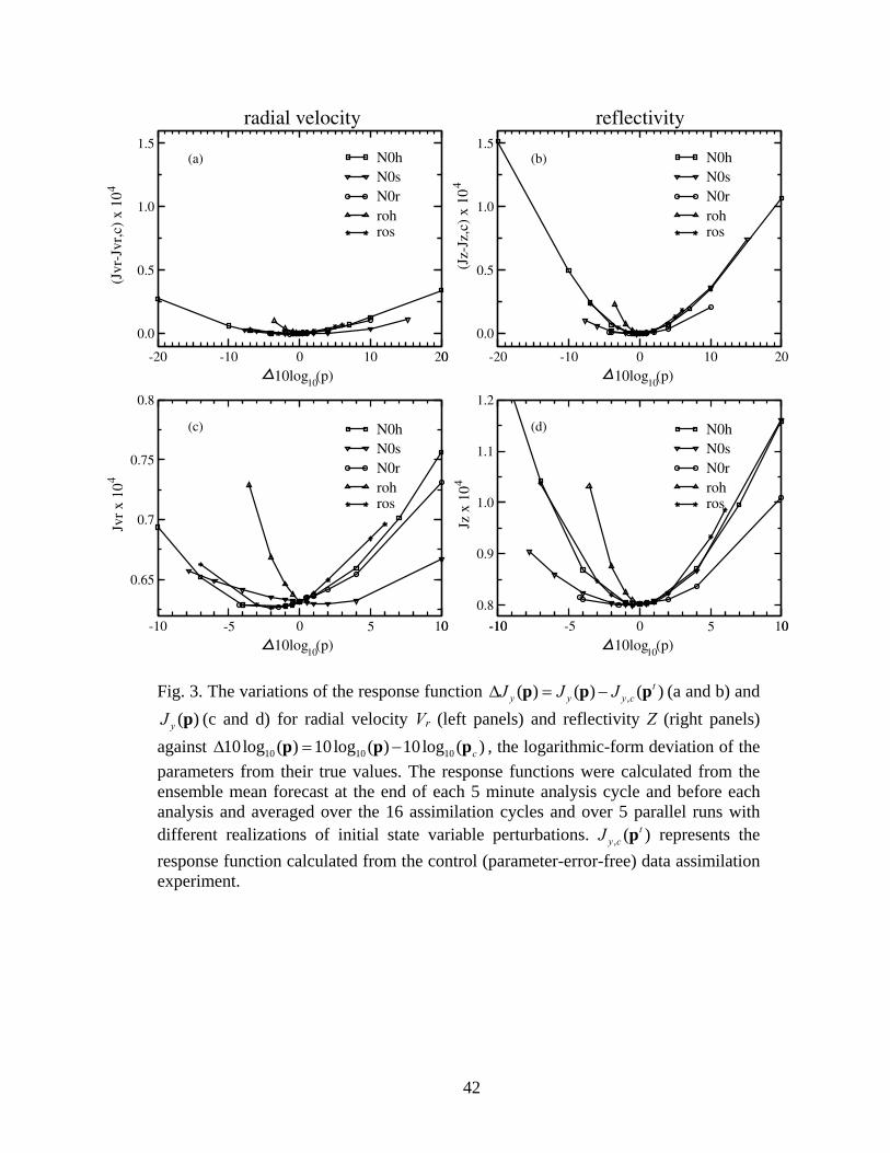
42
-20 -10 0 10 20
10log (p)
0.0
0.5
1.0
1.5
(Jvr
-Jvr
,c)
x 10
0
N0hN0sN0rrohros
-20 -10 0 10 20
10log (p)
0.0
0.5
1.0
1.5
(Jz-
Jz,c
) x
10
N0hN0sN0rrohros
-10 -5 0 5 10
10log (p)
0.65
0.7
0.75
0.8
Jvr
x 10
0
N0hN0sN0rrohros
-10 0 5 10
10log (p)
0.8
0.9
1.0
1.1
1.2
Jz x
10
-10 0
N0hN0sN0rrohros
-5
(a) (b)
(c) (d)
44 4
4
10
1010
10
radial velocity reflectivity
Fig. 3. The variations of the response function ,( ) ( ) ( )ty y y cJ J JΔ = −p p p (a and b) and
( )yJ p (c and d) for radial velocity Vr (left panels) and reflectivity Z (right panels) against 10 10 1010log ( ) 10log ( ) 10log ( )cΔ = −p p p , the logarithmic-form deviation of the parameters from their true values. The response functions were calculated from the ensemble mean forecast at the end of each 5 minute analysis cycle and before each analysis and averaged over the 16 assimilation cycles and over 5 parallel runs with different realizations of initial state variable perturbations. , ( )t
y cJ p represents the response function calculated from the control (parameter-error-free) data assimilation experiment.

43
0 10 20 30 40
1
1.05
1.1
1.15
Jz /
Jz,c
0 10 20 30 40
1
1.05
1.1
1.15
N0h14N0s16N0r36ρh576ρs63
0 10 20 30 401
1.2
1.4
1.6
Jz /
Jz,c
0 10 20 30 401
1.2
1.4
1.6N0h45N0s37N0r87ρh400ρs400
0 10 20 30 40
forecast time (min)
1
1.05
1.1
1.15
1.2
1.25
1.3
1.35Jz
/ Jz
,c
0 10 20 30 40
1
1.05
1.1
1.15
1.2
1.25
1.3
1.35
N0h14N0s16N0r36ρh576ρs63
0 10 20 30 40
forecast time (min)
1
1.2
1.4
1.6
1.8
2
2.2
Jz /
Jz,c
0 10 20 30 401
1.2
1.4
1.6
1.8
2
2.2
N0h45N0s37N0r87ρh400ρs400
(a) (b)
(c) (d)
Smaller deviation Larger deviation
Fig. 4. Time evolution of the ratios of the response functions for Z, of forecast sensitivity experiments (c.f., Table 2), to that of the CNTL forecast experiment,
,( ) / ( )z z cJ Jp p . The response functions are calculated against error-free reflectivity data in (a) and (b) and against error-containing reflectivity data in (c) and (d). Smaller parameter errors are used in (a) and (c) and larger ones are used in (b) and (d).

44
0
4
8
12
16z
(km
)
16 24 32 40 48 56 640
4
8
12
16
z (k
m)
16 24 32 40 48 56 64 16 24 32 40 48 56 64
qs (g/kg) MIN=0.00 MAX=2.63qh (g/kg) MIN=0.00 MAX=4.75qr (g/kg) MIN=0.00 MAX=4.06
dqs (g/kg) MIN=-.111 MAX=1.230dqh (g/kg) MIN=-1.72 MAX=0.606dqr (g/kg) MIN=-1.05 MAX=0.329
dqs (g/kg) MIN=-.855E-01 MAX=1.48dqh (g/kg) MIN=-.590 MAX=0.870E-01dqr (g/kg) MIN=-.104 MAX=0.983E-01
n0h = 4x10 (m )-43 n0s = 3x10 (m )-47CNTL
dqs (g/kg) MIN=-.544 MAX=0.117E-01dqh (g/kg) MIN=-.592E-01 MAX=0.705dqr (g/kg) MIN=-.162 MAX=1.30
dqs (g/kg) MIN=-.662 MAX=0.139E-01dqh (g/kg) MIN=-.754 MAX=2.01dqr (g/kg) MIN=-.775 MAX=0.322
dqs (g/kg) MIN=-.593 MAX=0.128dqh (g/kg) MIN=-.518 MAX=0.115E-01dqr (g/kg) MIN=-.333 MAX=0.121E-01
n0r = 8x10 (m )-47 ρh = 400 (kg m )-3 ρs = 400 (kg m )-3
x (km) x (km) x (km)
(a) (b) (c)
(d) (e) (f)
Fig. 5. Vertical cross sections of (a) mixing ratios (g kg-1): qr at intervals of 0.025, 0.1, 0.8, 2.5, 5.0 (thin gray), qh at intervals of 0.025, 0.1, 0.5, 1.0, 3.0, 5.0 (thick black) and qs at intervals of 0.05, 0.2, 0.5, 1.2, 2.0 (thick gray) for CNTL forecast experiment; and mixing ratio differences [ g kg-1; sensitivity experiment – CNTL; solid (dashed) contours represent positive (negative) values ] for qr at intervals of -0.6, -0.3, -0.1, -0.04, 0.015, 0.015, 0.08, 0.3, 0.6; qh at intervals of -1.5, -1.2, -0.8, -0.5, -0.2, -0.05, -0.025, 0.025, 0.05, 0.2, 0.5, 0.8, 1.2, 1.5 (thick black); qs at intervals of -1.5, -1.2, -0.6, -0.1, 0.025, 0.025, 0.1, 0.6, 1.2, 1.5 (thick brown) for forecast experiment (b) N0h43, (c) N0s37, (d) N0r87, (e) ρh400 and (f) ρs400 through the maximum updraft at 70t = min. The forecast experiments were initialized from the ensemble mean analysis of the CNTL experiment at t = 60 min. Irregular contour intervals are used to facilitate the comparison with the reflectivity in Fig. 6, which is a log function of the mixing ratios.

45
5.
15.
25.
35.
45.
55.
65.
75.
0
4
8
12
16
z (k
m)
16 24 32 40 48 56 640
4
8
12
16
z (k
m)
16 24 32 40 48 56 64 16 24 32 40 48 56 64
Ref (dBZ) MIN=0.000 MAX=58.20 dref(dB) MIN=-17.5 MAX=11.5 dref(dB) MIN=-12.5 MAX=5.77
x (km)dref(dB) MIN=-20.2 MAX=8.94
x (km)dref(dB) MIN=-23.5 MAX=13.5
x (km)drefdb(dB) MIN=-6.57 MAX=5.09
n0h = 4x10 (m )-43 n0s = 3x10 (m )-47
n0r = 8x10 (m )-47 ρh = 400 (kg m )-3 ρs = 400 (kg m )-3
CNTL
(a) (b) (c)
(d) (e) (f)
Fig. 6. Vertical cross sections of (a) reflectivity (dBZ) at intervals of 5 dBZ for CNTL forecast experiment, and reflectivity differences (sensitivity experiment – CNTL) at intervals of 26, 22, 18, 14, 10, 8, 6, 4, 2,0± ± ± ± ± ± ± ± ± dBZ [ solid (dashed) contours represent positive (negative) values ] through the maximum updraft at t = 70 min for forecast experiments (b) N0h43, (c) N0s37, (d) N0r87, (e) ρh400 and (f) ρs400.

46
0
4
8
12
16
x (km)
z (k
m)
x (km)
(a) (b)
16 24 32 40 48 56 64 16 24 32 40 48 56 64
drefdb(dBZ) MIN=-10.0 MAX=2.61 drefdb(dBZ) MIN=-3.32 MAX=2.11
Fig. 7. Reflectivity differences between the sensitivity experiments and CNTL (sensitivity minus CNTL) at contour levels of 26, 22, 18, 14, 10, 8, 6, 4, 2,0± ± ± ± ± ± ± ± ± dBZ [ solid (dashed) contours represent positive (negative) values ] through the maximum updraft at t = 70 min for forecast experiments (a) N0h43ρh400 with n0h = 4×10³ (m-4) and ρh = 400 (kg m-3) and (b) N0h43N0s55ρh400 with n0h = 4×10³ (m-4), n0s = 5×10⁵ (m-4), and ρh = 400 (kg m-3).

47
elevation 4.3deg
8
24
40
56
Zc(dBZ) MIN= 0.0 MAX=64.59Z-Zc(dBZ) MIN=-13.81 MAX=16.12
elevation 4.3deg
Zc(dBZ) MIN= 0.0 MAX=64.59Z-Zc(dBZ) MIN=-22.52 MAX= 4.41
elevation 0.5deg
Zc(dBZ) MIN= 0.0 MAX=55.12Z-Zc(dBZ) MIN=-16.98 MAX=13.68
elevation 4.3deg
Zc(dBZ) MIN= 0.0 MAX=64.59Z-Zc(dBZ) MIN=-18.73 MAX=14.72
elevation 4.3deg
5.
15.
25.
35.
45.
55.
65.
75.
Zc(dBZ) MIN= 0.0 MAX=64.59Z-Zc(dBZ) MIN=-12.47 MAX= 5.93
8 24 40 56
8
24
40
56
cor(N0h,Z) MIN= -0.88 MAX= 1.00
8 24 40 56
cor(N0s,Z) MIN= -0.99 MAX= 0.32
8 24 40 56
cor(N0r,Z) MIN= -0.93 MAX= 0.90
8 24 40 56
cor(rh,Z) MIN= -0.96 MAX= 0.91
8 24 40 56
5.
15.
25.
35.
45.
55.
65.
75.
cor(rs,Z) MIN= -0.93 MAX= 0.73
(a) (b) (c) (d) (e)
(f) (g) (h) (i) (j)
x (km) x (km) x (km) x (km) x (km)
y (k
m)
y (k
m)
n0h = 4x10 (m )-45 n0s = 3x10 (m )-47 n0r = 8x10 (m )-46 ρh = 400 (kg m )-3 ρs = 400 (kg m )-3
Fig. 8. Correlations [ solid (dash) contours represent positive (negative) values at intervals of 0.2 ] between forecast reflectivity at observation points where simulated reflectivity data is greater than 0 dBZ, and logarithmically transformed (f) n0h, (g) n0s, (h) n0r, (i) hρ and (j) sρ estimated from members of single-parameter forecast ensemble; and reflectivity difference [ thick solid (dash) contours represent positive (negative) values at intervals of 2dB ] between forecast sensitivity experiment (a) N0h45, (b) N0s37, (c) N0r87, (d) ρh400, (e) ρs400 and the CNTL forecast experiment at selected elevation levels at 70t = min. The shading and thin solid contours represent Z from the CNTL forecast experiment.

48
elevation 4.3deg
8 24 40 568
24
40
56
cor(N0h,Z) MIN= -0.84 MAX= 0.97
elevation 4.3deg
8 24 40 56
cor(N0s,Z) MIN= -0.86 MAX= 0.29
elevation 0.5deg
8 24 40 56
cor(N0r,Z) MIN= -0.85 MAX= 0.90
24
40
56
(a) (b) (c)
y (k
m)
x (km) x (km) x (km)
Fig. 9. Correlations [ thick contours, solid (dash) contours represent positive (negative) values at intervals of 0.2 ] between reflectivity and logarithmically transformed (a) n0h, (b) n0s, (c) n0r, estimated from members of the 3-parameter forecast ensemble at
70t = min. The shading and thin solid contours represent Z from the control forecast experiment.

49
elevation 4.3deg
8 24 40 568
24
40
56
cor(N0h,Z) MIN= -0.77 MAX= 0.90
elevation 4.3deg
8 24 40 568
24
40
56
cor(N0s,Z) MIN= -0.60 MAX= 0.28
elevation 0.5deg
8 24 40 568
24
40
56
cor(N0r,Z) MIN= -0.85 MAX= 0.90
elevation 4.3deg
8 24 40 568
24
40
56
cor(rh,Z) MIN= -0.45 MAX= 0.59
elevation 4.3deg
8 24 40 568
24
40
56
5.
15.
25.
35.
45.
55.
65.
75.
cor(rs,Z) MIN= -0.44 MAX= 0.64
(a) (b) (c) (d) (e)
x (km) x (km) x (km) x (km) x (km)
y (k
m)
Fig. 10. As in Fig. 9, but the correlation coefficients are estimated from the members of the 5-parameter forecast ensemble at t = 70 min.

50
Table 1. A summary of the uncertainty ranges, defined by the lower bound ip and upper bound ip , and the control (assumed true) values for intercept parameters n0h, n0s, n0r, and hail and snow densities hρ and sρ used in this study.
Parameter ip
ip
ip
Control values of parameters, icp
Hail/graupel intercept n0h (m-4) 4×10² 4×10⁶ 4×10⁴
Snow intercept n0s (m-4) 5×10⁵ 1×10⁸ 3×10⁶
Rain intercept n0r (m-4) 3×10⁶ 8×10⁷ 8×10⁶
Density of hail/graupel hρ ( kg m-3) 400 913 913
Density of snow sρ ( kg m-3) 20 400 100

51
Table 2. List of the parameters values, ip , and their logarithmical deviations from the true values, ( )1010log ipΔ , in the sensitivity experiments. The parameter that is changed from its true value is listed for the corresponding sensitivity experiment while other parameters used the true values.
Larger deviation Smaller deviation Parameter
Experiment ip ( )1010log ipΔ Experiment ip ( )1010 log ipΔ
n0h (m-4) N0h45 4×10⁵ 10 N0h14 1.59×10⁴ -4
n0s (m-4) N0s37 3×10⁷ 10 N0s16 1.19×10⁶ -4
n0r (m-4) N0r87 8×10⁷ 10 N0r36 3.18×10⁶ -4
hρ (kg m-3) ρh400 400 -3.58 hρ 576 576 -2
sρ (kg m-3) ρs400 400 6 sρ 63 63 -2

52
Table 3. Absolute values of correlations, averaged over observation points, at which Z > 0 dBZ, at t = 70 min, between forecast Z or Vr and one of the logarithmically transformed microphysical parameters as estimated from the forecast ensembles with different parameters perturbed from their true values, except sρ , which is perturbed from 700 kg m-3.
n0h n0s n0r hρ sρ Experiment
Z Vr Z Vr Z Vr Z Vr Z Vr
1-para 0.53 0.21 0.47 0.18 0.22 0.12 0.41 0.14 0.30 0.15
2-para ( 0 ,h hn ρ ) 0.49 0.20 0.20 0.13
2-para ( 0 ,s sn ρ ) 0.39 0.17 0.22 0.14
3-para
0 0( , , )r s sn n n
0.48 0.20 0.30 0.17 0.20 0.12
4-para
0 0( , , , )r s s hn n n ρ
0.45 0.20 0.27 0.17 0.19 0.12 0.21 0.13
5-para
(all five)
0.44 0.18 0.23 0.16 0.17 0.11 0.19 0.12 0.18 0.14