1

Simultaneous Contact, Gait and Motion Planningfor Robust Multi-Legged Locomotion via

Mixed-Integer Convex OptimizationBernardo Aceituno-Cabezas1, Carlos Mastalli2, Hongkai Dai3, Michele Focchi2, Andreea Radulescu2,

Darwin G. Caldwell2, Jose Cappelletto1, Juan C. Grieco1, Gerardo Fernandez-Lopez1, and Claudio Semini2

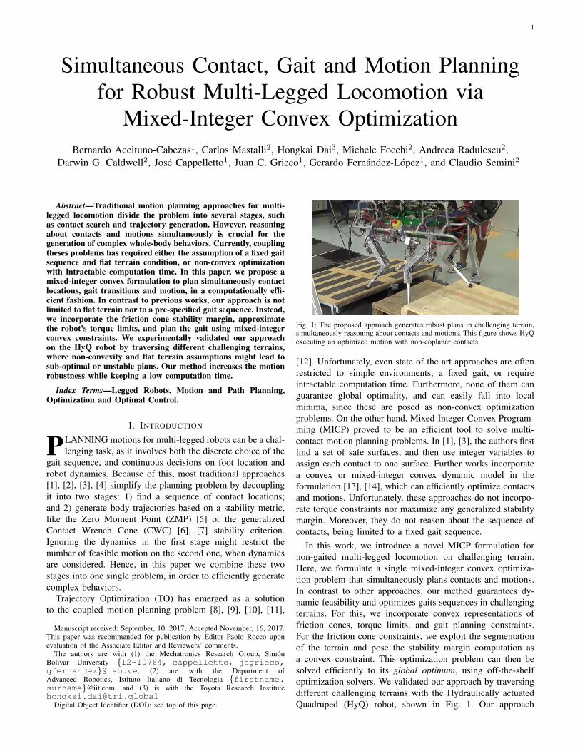
Abstract—Traditional motion planning approaches for multi-legged locomotion divide the problem into several stages, suchas contact search and trajectory generation. However, reasoningabout contacts and motions simultaneously is crucial for thegeneration of complex whole-body behaviors. Currently, couplingtheses problems has required either the assumption of a fixed gaitsequence and flat terrain condition, or non-convex optimizationwith intractable computation time. In this paper, we propose amixed-integer convex formulation to plan simultaneously contactlocations, gait transitions and motion, in a computationally effi-cient fashion. In contrast to previous works, our approach is notlimited to flat terrain nor to a pre-specified gait sequence. Instead,we incorporate the friction cone stability margin, approximatethe robot’s torque limits, and plan the gait using mixed-integerconvex constraints. We experimentally validated our approachon the HyQ robot by traversing different challenging terrains,where non-convexity and flat terrain assumptions might lead tosub-optimal or unstable plans. Our method increases the motionrobustness while keeping a low computation time.

Index Terms—Legged Robots, Motion and Path Planning,Optimization and Optimal Control.

I. INTRODUCTION

PLANNING motions for multi-legged robots can be a chal-lenging task, as it involves both the discrete choice of the

gait sequence, and continuous decisions on foot location androbot dynamics. Because of this, most traditional approaches[1], [2], [3], [4] simplify the planning problem by decouplingit into two stages: 1) find a sequence of contact locations;and 2) generate body trajectories based on a stability metric,like the Zero Moment Point (ZMP) [5] or the generalizedContact Wrench Cone (CWC) [6], [7] stability criterion.Ignoring the dynamics in the first stage might restrict thenumber of feasible motion on the second one, when dynamicsare considered. Hence, in this paper we combine these twostages into one single problem, in order to efficiently generatecomplex behaviors.

Trajectory Optimization (TO) has emerged as a solutionto the coupled motion planning problem [8], [9], [10], [11],

Manuscript received: September, 10, 2017; Accepted November, 16, 2017.This paper was recommended for publication by Editor Paolo Rocco uponevaluation of the Associate Editor and Reviewers’ comments.

The authors are with (1) the Mechatronics Research Group, SimonBolıvar University {12-10764, cappelletto, jcgrieco,gfernandez}@usb.ve, (2) are with the Department ofAdvanced Robotics, Istituto Italiano di Tecnologia {firstname.surname}@iit.com, and (3) is with the Toyota Research Institutehongkai.dai@tri.global

Digital Object Identifier (DOI): see top of this page.

Fig. 1: The proposed approach generates robust plans in challenging terrain,simultaneously reasoning about contacts and motions. This figure shows HyQexecuting an optimized motion with non-coplanar contacts.

[12]. Unfortunately, even state of the art approaches are oftenrestricted to simple environments, a fixed gait, or requireintractable computation time. Furthermore, none of them canguarantee global optimality, and can easily fall into localminima, since these are posed as non-convex optimizationproblems. On the other hand, Mixed-Integer Convex Program-ming (MICP) proved to be an efficient tool to solve multi-contact motion planning problems. In [1], [3], the authors firstfind a set of safe surfaces, and then use integer variables toassign each contact to one surface. Further works incorporatea convex or mixed-integer convex dynamic model in theformulation [13], [14], which can efficiently optimize contactsand motions. Unfortunately, these approaches do not incorpo-rate torque constraints nor maximize any generalized stabilitymargin. Moreover, they do not reason about the sequence ofcontacts, being limited to a fixed gait sequence.

In this work, we introduce a novel MICP formulation fornon-gaited multi-legged locomotion on challenging terrain.Here, we formulate a single mixed-integer convex optimiza-tion problem that simultaneously plans contacts and motions.In contrast to other approaches, our method guarantees dy-namic feasibility and optimizes gaits sequences in challengingterrains. For this, we incorporate convex representations offriction cones, torque limits, and gait planning constraints.For the friction cone constraints, we exploit the segmentationof the terrain and pose the stability margin computation asa convex constraint. This optimization problem can then besolved efficiently to its global optimum, using off-the-shelfoptimization solvers. We validated our approach by traversingdifferent challenging terrains with the Hydraulically actuatedQuadruped (HyQ) robot, shown in Fig. 1. Our approach

2

Optimal

Plan

Goal

StateConvex terrain

segmentation

Current

State

Command

Simultaneous

Contact and Motion

Planner

Whole-body

Controller

Fig. 2: Overview of our convex trajectory optimization approach. Here, wecompute contact locations and motions within a single mixed-integer convexprogram, given a goal state and a convex segmentation of the safe terrain.

generates robust motions, even during gait transitions and non-coplanar contact scenarios.

The rest of this paper is organized as follows: SectionII presents our simultaneous contact and motion planningapproach. Section III presents our whole-body controller.Section IV presents a set of experiments on HyQ traversingchallenging terrains, and Section V discusses and concludeson the contributions of this work.

II. SIMULTANEOUS CONTACT AND MOTION PLANNING

In this section, we describe our formulation of the simul-taneous contact and motion planning problem using Mixed-Integer Convex Optimization.

A. Approach Overview

Let us consider a robot with nl legs and a locomotion plan,discretized on N time-knots. We formulate a MICP to find theoptimal contact locations and motions, given a goal positionrG and a convex segmentation of the terrain. An illustrationof this approach is shown in Fig. 2.

We describe the dynamic evolution of the system witha centroidal model (Section II-B). We include gait plan-ning as part of the optimization (Section II-C), describingthe motion through time-slots over which legs swing. Thisevolution is subject to robot and environmental constraintssuch as: approximated kinematic reachability (Section II-D),friction cone constraints (Section II-F), and approximatedtorque limits (Section II-H). describing the motion throughtime-slots over which we will generate leg swings. We adoptthe formulation in [13] to further address the non-linearities ofthe angular dynamics by relying on a convex decompositionof bilinear terms, making our optimization problem convex(Section II-G).

B. Centroidal Dynamics

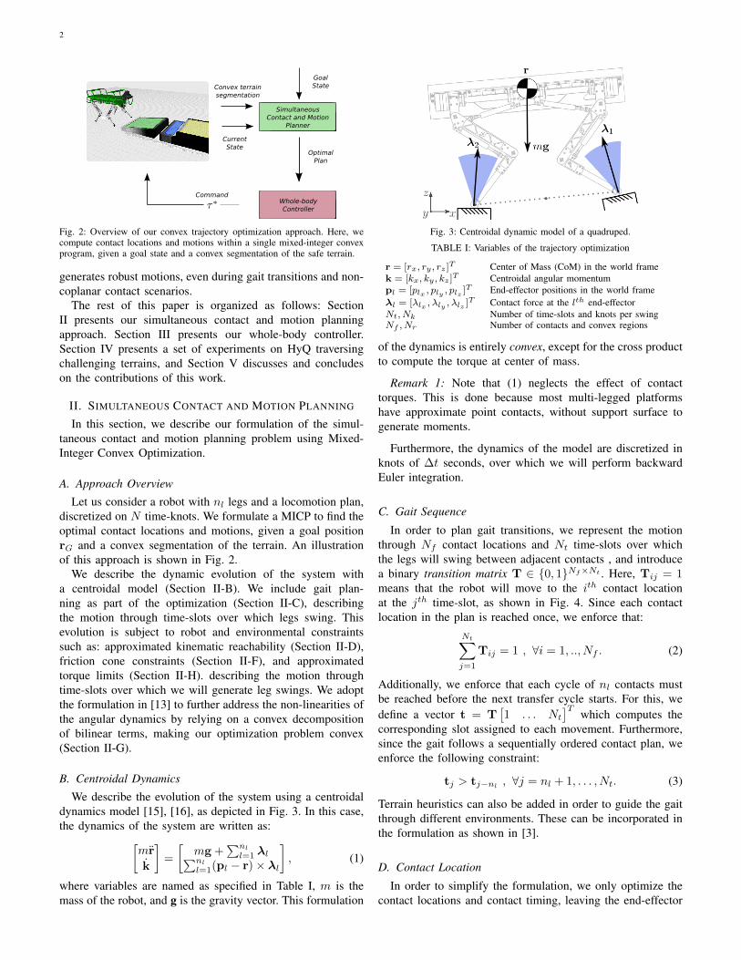
We describe the evolution of the system using a centroidaldynamics model [15], [16], as depicted in Fig. 3. In this case,the dynamics of the system are written as:[

mr

k

]=

[mg +

∑nl

l=1 λl∑nl

l=1(pl − r)× λl

], (1)

where variables are named as specified in Table I, m is themass of the robot, and g is the gravity vector. This formulation

Fig. 3: Centroidal dynamic model of a quadruped.

TABLE I: Variables of the trajectory optimization

r = [rx, ry , rz ]T Center of Mass (CoM) in the world framek = [kx, ky , kz ]T Centroidal angular momentumpl = [plx , ply , plz ]

T End-effector positions in the world frameλl = [λlx , λly , λlz ]

T Contact force at the lth end-effectorNt, Nk Number of time-slots and knots per swingNf , Nr Number of contacts and convex regions

of the dynamics is entirely convex, except for the cross productto compute the torque at center of mass.

Remark 1: Note that (1) neglects the effect of contacttorques. This is done because most multi-legged platformshave approximate point contacts, without support surface togenerate moments.

Furthermore, the dynamics of the model are discretized inknots of ∆t seconds, over which we will perform backwardEuler integration.

C. Gait Sequence

In order to plan gait transitions, we represent the motionthrough Nf contact locations and Nt time-slots over whichthe legs will swing between adjacent contacts , and introducea binary transition matrix T ∈ {0, 1}Nf×Nt . Here, Tij = 1means that the robot will move to the ith contact locationat the jth time-slot, as shown in Fig. 4. Since each contactlocation in the plan is reached once, we enforce that:

Nt∑j=1

Tij = 1 , ∀i = 1, .., Nf . (2)

Additionally, we enforce that each cycle of nl contacts mustbe reached before the next transfer cycle starts. For this, wedefine a vector t = T

[1 . . . Nt

]Twhich computes the

corresponding slot assigned to each movement. Furthermore,since the gait follows a sequentially ordered contact plan, weenforce the following constraint:

tj > tj−nl, ∀j = nl + 1, . . . , Nt. (3)

Terrain heuristics can also be added in order to guide the gaitthrough different environments. These can be incorporated inthe formulation as shown in [3].

D. Contact Location

In order to simplify the formulation, we only optimize thecontact locations and contact timing, leaving the end-effector

3

Fig. 4: Gait transition matrix and equivalent phase diagram. R, L,H and F represent right, left, hind and front supports.

Fig. 5: Left: Convex segmentation of safe contact surfaces. Right: Approximatekinematic reachability constraints.

trajectory as an interpolation between adjacent contacts in theplan. Since swing phases do not contribute to the centroidaldynamics, as force in the leg becomes null, this simplificationhas no effect on the resulting plan.

As part of the decision variables, we describe contactlocations for nl end-effectors using an array of Nf vectorsin R4, ordered by end-effector number, of the form:

f = (fx, fy, fz, θ),

representing the position of each contact in Cartesian spaceand the yaw orientation of the trunk when transitioning tothat contact, neglecting roll and pitch positions.

1) Safe-region assignment: Here, we will invert the prob-lem of avoiding obstacles by constraining the contacts to liewithin one of Nr convex safe contact surfaces, shown coloredin Fig. 5 (left). Each surface is represented as a polygonR = {c ∈ R3|Arc ≤ br}. The assignment of contactsto these surfaces is done through a binary decision matrixH ∈ {0, 1}Nf×Nr . The constraints, for the ith contact, are:

Nr∑r=1

Hir = 1, (4)

Hir ⇒ Arfi ≤ br, (5)

where the ⇒ (implies) operator is represented with big-Mformulation [17]. Such surfaces can be easily obtained withsegmentation algorithms.

2) Kinematic constraints: In order to ensure kinematicreachability, we must account for the workspace of eachindependent leg. To do this, we constrain each contact locationwithin the biggest square inscribed in the leg workspace, asshown in Fig. 5 (right). Algebraically:∣∣∣∣fi − [rT (i) + Li

(cos(θi + φi)sin(θi + φi)

)]∣∣∣∣ ≤ dlim, (6)

where rT (i) is the CoM location after transitioning to thecontact (given by the gait matrix T(i)), dlim is the squarediagonal, Li is the approximate distance from the trunk tothe leg, and φi is a known offset for each foot. Here, thetrigonometric functions are decomposed in terms piecewiselinear approximations of the trunk orientation functions.

To have them expressed as mixed-integer convex, we willfollow the approach of [1] and replace the trigonometric

functions of (6) with piecewise linear approximations of Nssegments s and c. We define binary matrices S and C in{0, 1}Nf×Ns to assign linear segments, which is done withthe following constraints:

Ns∑s=1

Sis = 1

Ns∑s=1

Cis = 1, (7)

Sik ⇒

{ψk−1 ≤ θi ≤ ψksi = mskθi + nsk

Cik ⇒

{γk−1 ≤ θi ≤ γkci = mckθi + nck

,

(8)where ψ and γ represent the boundaries between each linearsegment, and m and n represent its slope and intersection.

E. End-effector Trajectories

As mentioned in Section II-D, the end-effector trajectoriesare defined by the gait transition matrix T. For simplicity, wedefine the function γ(j, t) to reference the knots over whichan end-effector swings between two adjacent contacts in theplan, where j indicates the time-slot used for the swing andt ∈ [1, . . . , Nk] indicates the knot, where Nk is the number ofknots allocated for each slot. Then, the end-effector motionsare governed by the following constraint:

Tij ⇒ pl(i)γ(j,Nk) = fi, (9)

where l(i) is the leg number for the ith contact. This constraintenforces that the leg reaches the contact position fi at the endof the jth slot. Also, it is important to constrain that the legremains stationary when there is no transition. This is enforcedusing the following constraint over the lth leg:∑i∈C(l)

Tij = 0⇒ plγ(j,t) = plγ(j,1) ∀t ∈ [2, . . . , Nk], (10)

where C(l) are the contact indexes assigned to the lthleg. Fur-ther constraints can be added to make the end-effector followa specific swing trajectory. Moreover, we ensure kinematicfeasibility by constraining the CoM position with respect tothe end-effectors (Fig. 6). Here, we use the bounding boxconstraint:

d− < rj −∑nl

l=1 pljnl

< d+, (11)

where d− and d+ are the bounding box limits.

4

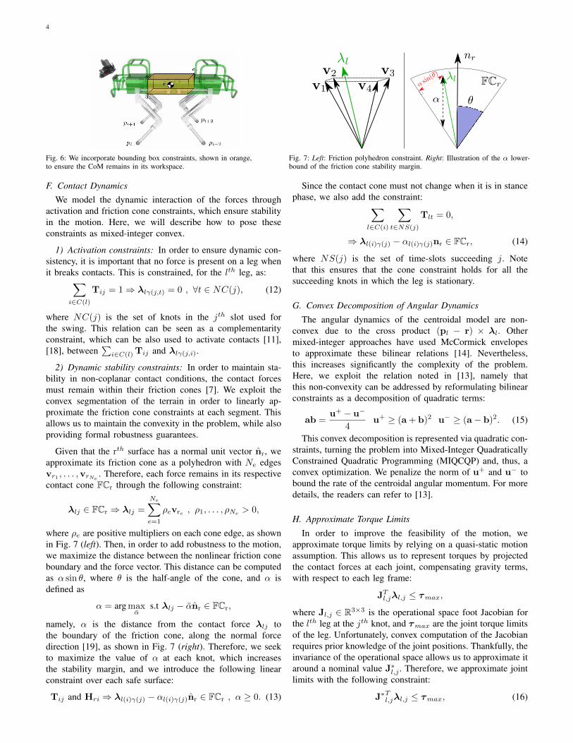
Fig. 6: We incorporate bounding box constraints, shown in orange,to ensure the CoM remains in its workspace.

Fig. 7: Left: Friction polyhedron constraint. Right: Illustration of the α lower-bound of the friction cone stability margin.

F. Contact DynamicsWe model the dynamic interaction of the forces through

activation and friction cone constraints, which ensure stabilityin the motion. Here, we will describe how to pose theseconstraints as mixed-integer convex.

1) Activation constraints: In order to ensure dynamic con-sistency, it is important that no force is present on a leg whenit breaks contacts. This is constrained, for the lth leg, as:∑

i∈C(l)

Tij = 1⇒ λlγ(j,t) = 0 , ∀t ∈ NC(j), (12)

where NC(j) is the set of knots in the jth slot used forthe swing. This relation can be seen as a complementarityconstraint, which can be also used to activate contacts [11],[18], between

∑i∈C(l) Tij and λlγ(j,i).

2) Dynamic stability constraints: In order to maintain sta-bility in non-coplanar contact conditions, the contact forcesmust remain within their friction cones [7]. We exploit theconvex segmentation of the terrain in order to linearly ap-proximate the friction cone constraints at each segment. Thisallows us to maintain the convexity in the problem, while alsoproviding formal robustness guarantees.

Given that the rth surface has a normal unit vector nr, weapproximate its friction cone as a polyhedron with Ne edgesvr1 , . . . ,vrNe

. Therefore, each force remains in its respectivecontact cone FCr through the following constraint:

λlj ∈ FCr ⇒ λlj =

Ne∑e=1

ρevre , ρ1, . . . , ρNe > 0,

where ρe are positive multipliers on each cone edge, as shownin Fig. 7 (left). Then, in order to add robustness to the motion,we maximize the distance between the nonlinear friction coneboundary and the force vector. This distance can be computedas α sin θ, where θ is the half-angle of the cone, and α isdefined as

α = arg maxα

s.t λlj − αnr ∈ FCr,

namely, α is the distance from the contact force λlj tothe boundary of the friction cone, along the normal forcedirection [19], as shown in Fig. 7 (right). Therefore, we seekto maximize the value of α at each knot, which increasesthe stability margin, and we introduce the following linearconstraint over each safe surface:

Tij and Hri ⇒ λl(i)γ(j) − αl(i)γ(j)nr ∈ FCr , α ≥ 0. (13)

Since the contact cone must not change when it is in stancephase, we also add the constraint:∑

l∈C(i)

∑t∈NS(j)

Tlt = 0,

⇒ λl(i)γ(j) − αl(i)γ(j)nr ∈ FCr, (14)

where NS(j) is the set of time-slots succeeding j. Notethat this ensures that the cone constraint holds for all thesucceeding knots in which the leg is stationary.

G. Convex Decomposition of Angular Dynamics

The angular dynamics of the centroidal model are non-convex due to the cross product (pl − r) × λl. Othermixed-integer approaches have used McCormick envelopesto approximate these bilinear relations [14]. Nevertheless,this increases significantly the complexity of the problem.Here, we exploit the relation noted in [13], namely thatthis non-convexity can be addressed by reformulating bilinearconstraints as a decomposition of quadratic terms:

ab =u+ − u−

4u+ ≥ (a + b)2 u− ≥ (a− b)2. (15)

This convex decomposition is represented via quadratic con-straints, turning the problem into Mixed-Integer QuadraticallyConstrained Quadratic Programming (MIQCQP) and, thus, aconvex optimization. We penalize the norm of u+ and u− tobound the rate of the centroidal angular momentum. For moredetails, the readers can refer to [13].

H. Approximate Torque Limits

In order to improve the feasibility of the motion, weapproximate torque limits by relying on a quasi-static motionassumption. This allows us to represent torques by projectedthe contact forces at each joint, compensating gravity terms,with respect to each leg frame:

JTl,jλl,j ≤ τmax,

where Jl,j ∈ R3×3 is the operational space foot Jacobian forthe lth leg at the jth knot, and τmax are the joint torque limitsof the leg. Unfortunately, convex computation of the Jacobianrequires prior knowledge of the joint positions. Thankfully, theinvariance of the operational space allows us to approximate itaround a nominal value J∗l,j . Therefore, we approximate jointlimits with the following constraint:

J∗Tl,jλl,j ≤ τmax, (16)

5

This constraint approximates the Actuation Wrench Poly-tope (AWP) to define an approximation of the Feasible WrenchPolytope (FWP), as defined in [20]. In practice, this approx-imation is useful for most motions, close to the nominalposition and without aggressive speeds. For further precision,one could use robust optimization [21] to constrain over thevariations of the Jacobian J∗l,j ± δJl,j .

I. Trajectory Optimization

Given the constraints stated above, we formulate a convextrajectory optimization, as follows:

minr,ko,pl,λl

gT +

N∑k=1

g(k),

where T is the total number of knots, g(k) is a running costalong the plan and gT is a terminal cost. Our running costg(k) maximizes the stability of the motion, while seeking forthe fastest and smoothest gait. For this, the objectives are:

1) Minimize the CoM acceleration r.2) Minimize the contact forces magnitude ‖λ‖.3) Minimize the upper bound of quadratic terms U =

(u−,u+) used in the convex angular dynamics model.4) Maximize the stability margin α.5) Minimize the execution time, by minimizing the sum of

the elements in the time vector t.The running cost g(k) is defined as:

g(k) = ‖rk‖Qv + ‖λl,k‖QF+ quUk + qttk − qααk,

On the other hand, the terminal cost gT biases the plantowards its goal, the terminal position rG, as:

gT = ‖rT − rG‖Qg , (17)

where q are positive weights, Q are positive-semidefiniteweighting matrices, and ‖v‖Q stands for the weightedsquared-L2 norm vTQv. In practice, we add a small costto ‖k‖Qk

in order to generate smoother motions.

III. WHOLE-BODY CONTROL

The CoM motion, body attitude and swing motions arecontrolled by a trunk controller. It computes the feed-forwardjoint torques τ ∗ff necessary to achieve a desired motionwithout violating friction, torques or kinematic limits. Toaddress unpredictable events (e.g. limit foot divergence in caseof slippage on an unknown surface), an impedance controllercomputes in parallel the feedback joint torques τ fb from thedesired joint motion (qdj , q

dj ). Note that the desired body and

joint motions have to be consistent with each other in orderto prevent conflicts with the trunk controller.

To achieve compliantly desired trunk motions, we computea reference CoM acceleration (rr ∈ R3) and body angularacceleration (ωrb ∈ R3) through a virtual model:

rr = rd + Kr(rd − r) + Dr(r

d − r),

ωrb = ωdb + Kθe(RdbR

Tb ) + Dθ(ω

db − ωb), (18)

where (rd, rd, rd) ∈ R3 are the desired CoM position,velocity and acceleration respectively, e(·) : R3×3 → R3

is a mapping from the rotation matrix into the associatedrotation vector, ωb ∈ R3 is the angular velocity of thetrunk. Kr,Dr,Kθ,Dθ ∈ R3×3 are positive-definite diagonalmatrices of proportional and derivative gains, respectively.

The target of our trunk controller is to minimize the errorbetween the reference and actual accelerations while enforc-ing friction, torque and kinematic constraints. As mentionedabove, the reference accelerations are computed from (18).We formulate the problem using Quadratic Programming (QP)with the generalized accelerations and the contact forces asdecision variables, i.e. x = [qT ,λT ]T ∈ R6+n+3nl :

x∗ = arg minxgerr(x) + ‖x‖W

s. t. Ax = b

d < Cx < d

(19)

where n represents the number of active Degrees of Freedom(DoFs). The first term of the cost function (19) penalizes thetracking error:

gerr(x) =

∥∥∥∥ r− rr

ωb − ωrb

∥∥∥∥S

, (20)

while the second one is a regularization factor to keep thesolution bounded or to pursue additional criteria. Both costsare quadratic-weighted terms. As the CoM acceleration is nota decision variable, we compute them from the contact forcesusing the centroidal dynamic model. We then re-write thetracking cost (20) as ‖Gx− g0‖ where:

G =

[03×3 03×3 03×n

1mI1 · · · 1

mInl

03×3 13×3 03×n 03×3nl

],g0 =

[rr + gωrb

],

and Ik representing an identity matrix for the kth end-effector. The equality constraints Ax = b encodes dynamicconsistency, stance condition and swing task. On the otherhand, the inequality constraints d < Cx < d encode friction,torque, and kinematic limits.

We map the optimal solution x∗ into desired feed-forwardjoint torques τ ∗ff ∈ Rn using the actuated part of the fulldynamics of the robot as:

τ ∗ff =[MT

bj Mj

]q∗ + hj − JTcjλ

∗ (21)

where Mbj ∈ R(6+n)×n represents the coupled inertia be-tween the floating-base and joints, Mj ∈ Rn×n the jointcontribution to the inertia matrix, hj ∈ Rn is the force vectorthat accounts for Coriolis, centrifugal, and gravitational forcesto the joint torque, and Jcj ∈ R3nl×n is a stack of Jacobiansof the nl end-effectors.

Finally, the feed-forward torques τ ∗ff are summed with thejoint PD torques (i.e. feedback torques τ fb) to form the desiredtorque command τ d:

τ d = τ ∗ff + PD(qdj , qdj ), (22)

which is sent to a low-level joint-torque controller. For moreinformation on this controller the reader can refer to [22]

6

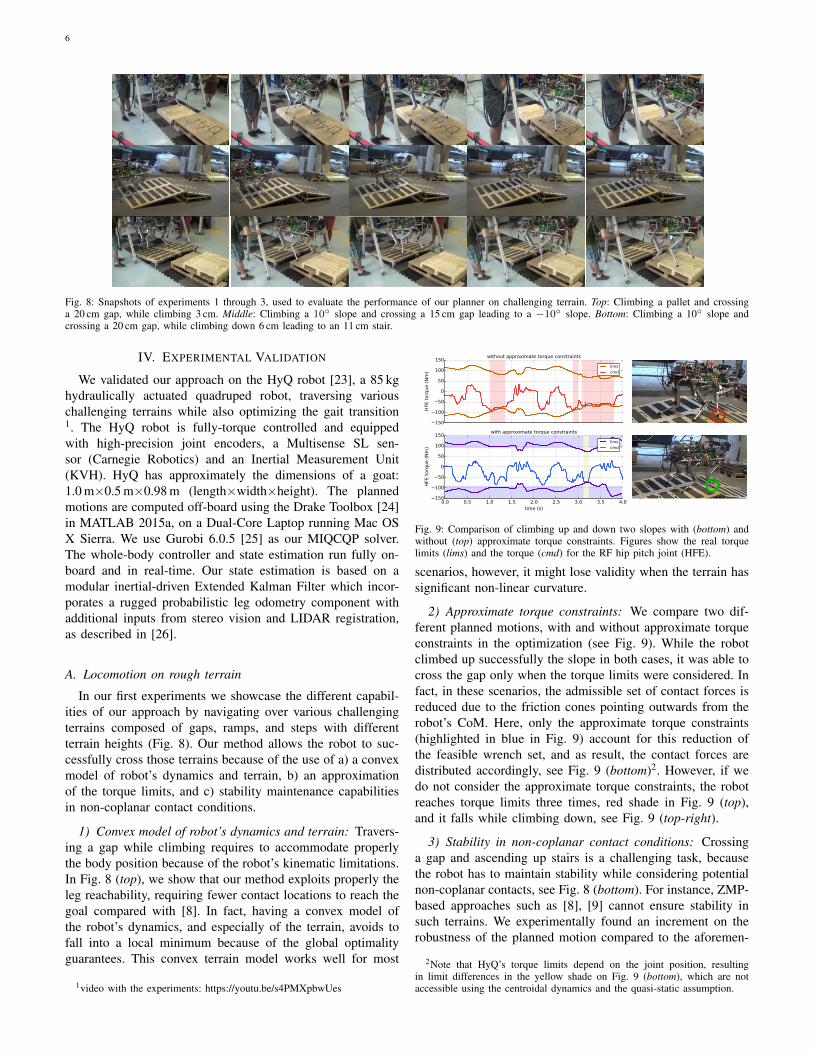
Fig. 8: Snapshots of experiments 1 through 3, used to evaluate the performance of our planner on challenging terrain. Top: Climbing a pallet and crossinga 20 cm gap, while climbing 3 cm. Middle: Climbing a 10◦ slope and crossing a 15 cm gap leading to a −10◦ slope. Bottom: Climbing a 10◦ slope andcrossing a 20 cm gap, while climbing down 6 cm leading to an 11 cm stair.

IV. EXPERIMENTAL VALIDATION

We validated our approach on the HyQ robot [23], a 85 kghydraulically actuated quadruped robot, traversing variouschallenging terrains while also optimizing the gait transition1. The HyQ robot is fully-torque controlled and equippedwith high-precision joint encoders, a Multisense SL sen-sor (Carnegie Robotics) and an Inertial Measurement Unit(KVH). HyQ has approximately the dimensions of a goat:1.0 m×0.5 m×0.98 m (length×width×height). The plannedmotions are computed off-board using the Drake Toolbox [24]in MATLAB 2015a, on a Dual-Core Laptop running Mac OSX Sierra. We use Gurobi 6.0.5 [25] as our MIQCQP solver.The whole-body controller and state estimation run fully on-board and in real-time. Our state estimation is based on amodular inertial-driven Extended Kalman Filter which incor-porates a rugged probabilistic leg odometry component withadditional inputs from stereo vision and LIDAR registration,as described in [26].

A. Locomotion on rough terrain

In our first experiments we showcase the different capabil-ities of our approach by navigating over various challengingterrains composed of gaps, ramps, and steps with differentterrain heights (Fig. 8). Our method allows the robot to suc-cessfully cross those terrains because of the use of a) a convexmodel of robot’s dynamics and terrain, b) an approximationof the torque limits, and c) stability maintenance capabilitiesin non-coplanar contact conditions.

1) Convex model of robot’s dynamics and terrain: Travers-ing a gap while climbing requires to accommodate properlythe body position because of the robot’s kinematic limitations.In Fig. 8 (top), we show that our method exploits properly theleg reachability, requiring fewer contact locations to reach thegoal compared with [8]. In fact, having a convex model ofthe robot’s dynamics, and especially of the terrain, avoids tofall into a local minimum because of the global optimalityguarantees. This convex terrain model works well for most

1video with the experiments: https://youtu.be/s4PMXpbwUes

150

100

50

0

50

100

150

HFE t

orq

ue (

Nm

)

without approximate torque constraints

lims

cmd

0.0 0.5 1.0 1.5 2.0 2.5 3.0 3.5 4.0

time (s)

150

100

50

0

50

100

150

HFE

torq

ue (

Nm

)

with approximate torque constraints

lims

cmd

Fig. 9: Comparison of climbing up and down two slopes with (bottom) andwithout (top) approximate torque constraints. Figures show the real torquelimits (lims) and the torque (cmd) for the RF hip pitch joint (HFE).

scenarios, however, it might lose validity when the terrain hassignificant non-linear curvature.

2) Approximate torque constraints: We compare two dif-ferent planned motions, with and without approximate torqueconstraints in the optimization (see Fig. 9). While the robotclimbed up successfully the slope in both cases, it was able tocross the gap only when the torque limits were considered. Infact, in these scenarios, the admissible set of contact forces isreduced due to the friction cones pointing outwards from therobot’s CoM. Here, only the approximate torque constraints(highlighted in blue in Fig. 9) account for this reduction ofthe feasible wrench set, and as result, the contact forces aredistributed accordingly, see Fig. 9 (bottom)2. However, if wedo not consider the approximate torque constraints, the robotreaches torque limits three times, red shade in Fig. 9 (top),and it falls while climbing down, see Fig. 9 (top-right).

3) Stability in non-coplanar contact conditions: Crossinga gap and ascending up stairs is a challenging task, becausethe robot has to maintain stability while considering potentialnon-coplanar contacts, see Fig. 8 (bottom). For instance, ZMP-based approaches such as [8], [9] cannot ensure stability insuch terrains. We experimentally found an increment on therobustness of the planned motion compared to the aforemen-

2Note that HyQ’s torque limits depend on the joint position, resultingin limit differences in the yellow shade on Fig. 9 (bottom), which are notaccessible using the centroidal dynamics and the quasi-static assumption.

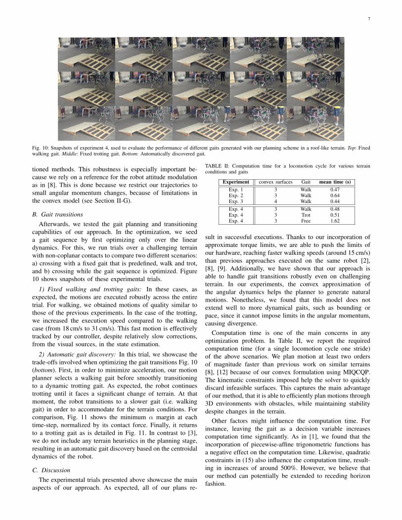
7

Fig. 10: Snapshots of experiment 4, used to evaluate the performance of different gaits generated with our planning scheme in a roof-like terrain. Top: Fixedwalking gait. Middle: Fixed trotting gait. Bottom: Automatically discovered gait.

tioned methods. This robustness is especially important be-cause we rely on a reference for the robot attitude modulationas in [8]. This is done because we restrict our trajectories tosmall angular momentum changes, because of limitations inthe convex model (see Section II-G).

B. Gait transitionsAfterwards, we tested the gait planning and transitioning

capabilities of our approach. In the optimization, we seeda gait sequence by first optimizing only over the lineardynamics. For this, we run trials over a challenging terrainwith non-coplanar contacts to compare two different scenarios:a) crossing with a fixed gait that is predefined, walk and trot,and b) crossing while the gait sequence is optimized. Figure10 shows snapshots of these experimental trials.

1) Fixed walking and trotting gaits: In these cases, asexpected, the motions are executed robustly across the entiretrial. For walking, we obtained motions of quality similar tothose of the previous experiments. In the case of the trotting,we increased the execution speed compared to the walkingcase (from 18 cm/s to 31 cm/s). This fast motion is effectivelytracked by our controller, despite relatively slow corrections,from the visual sources, in the state estimation.

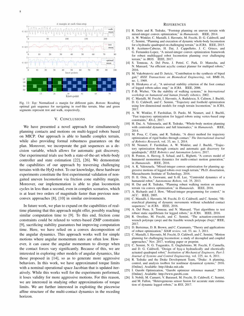
2) Automatic gait discovery: In this trial, we showcase thetrade-offs involved when optimizing the gait transitions Fig. 10(bottom). First, in order to minimize acceleration, our motionplanner selects a walking gait before smoothly transitioningto a dynamic trotting gait. As expected, the robot continuestrotting until it faces a significant change of terrain. At thatmoment, the robot transitions to a slower gait (i.e. walkinggait) in order to accommodate for the terrain conditions. Forcomparison, Fig. 11 shows the minimum α margin at eachtime-step, normalized by its contact force. Finally, it returnsto a trotting gait as is detailed in Fig. 11. In contrast to [3],we do not include any terrain heuristics in the planning stage,resulting in an automatic gait discovery based on the centroidaldynamics of the robot.

C. DiscussionThe experimental trials presented above showcase the main

aspects of our approach. As expected, all of our plans re-

TABLE II: Computation time for a locomotion cycle for various terrainconditions and gaits

Experiment convex surfaces Gait mean time (s)Exp. 1 3 Walk 0.47Exp. 2 3 Walk 0.64Exp. 3 4 Walk 0.44Exp. 4 3 Walk 0.48Exp. 4 3 Trot 0.51Exp. 4 3 Free 1.62

sult in successful executions. Thanks to our incorporation ofapproximate torque limits, we are able to push the limits ofour hardware, reaching faster walking speeds (around 15 cm/s)than previous approaches executed on the same robot [2],[8], [9]. Additionally, we have shown that our approach isable to handle gait transitions robustly even on challengingterrain. In our experiments, the convex approximation ofthe angular dynamics helps the planner to generate naturalmotions. Nonetheless, we found that this model does notextend well to more dynamical gaits, such as bounding orpace, since it cannot impose limits in the angular momentum,causing divergence.

Computation time is one of the main concerns in anyoptimization problem. In Table II, we report the requiredcomputation time (for a single locomotion cycle one stride)of the above scenarios. We plan motion at least two ordersof magnitude faster than previous work on similar terrains[8], [12] because of our convex formulation using MIQCQP.The kinematic constraints imposed help the solver to quicklydiscard infeasible surfaces. This captures the main advantageof our method, that it is able to efficiently plan motions through3D environments with obstacles, while maintaining stabilitydespite changes in the terrain.

Other factors might influence the computation time. Forinstance, leaving the gait as a decision variable increasescomputation time significantly. As in [1], we found that theincorporation of piecewise-affine trigonometric functions hasa negative effect on the computation time. Likewise, quadraticconstraints in (15) also influence the computation time, result-ing in increases of around 500%. However, we believe thatour method can potentially be extended to receding horizonfashion.

8

0 50 100 150 2000

0.5

1

αα margin at each time-step

walk

mean

0 10 20 30 40 50 60 70 800

0.5

1

α

trot

mean

0 10 20 30 40 50 60 70 80 90 100

knot-points

0

0.5

1

α

optimal

mean

Fig. 11: Top: Normalized α margin for different gaits. Bottom: Resultingoptimal gait sequence for navigating in roof-like terrain, blue and greensegments represent trot and walk, respectively.

V. CONCLUSIONS

We have presented a novel approach for simultaneouslyplanning contacts and motions on multi-legged robots basedon MICP. Our approach is able to handle complex terrain,while also providing formal robustness guarantees on theplan. Moreover, we incorporate the gait sequences as a de-cision variable, which allows for automatic gait discovery.Our experimental trials use both a state-of-the-art whole-bodycontroller and state estimation [22], [26]. We demonstratethe capabilities of our approach by traversing challengingterrains with the HyQ robot. To our knowledge, these hardwareexperiments constitute the first experimental validation of non-gaited uneven locomotion via friction cone stability margin.Moreover, our implementation is able to plan locomotioncycles in less than a second, even in complex scenarios, whichis at least two orders of magnitude faster than previous non-convex approaches [8], [10] in similar environments.

In future work, we plan to expand on the capabilities of real-time planning that this approach might offer, possibly reachingsimilar computation time to [9]. To this end, friction coneconstraints could be relaxed to vertex-based ZMP constraints[9], sacrificing stability guarantees but improving computationtime. Here, we have relied on a convex decomposition ofthe angular dynamics. This approach works well for simplemotions where angular momentum rates are often low. How-ever, it can cause the angular momentum to diverge whenthe contact forces vary significantly. Because of this, we areinterested in exploring other models of angular dynamics, likethose proposed in [14], so as to generate more aggressivebehaviors. In this work, we have approximated torque limitswith a nominal operational space Jacobian that is updated iter-atively. While this works well for the experiments performed,it loses validity for more aggressive motions. For this reason,we are interested in studying other approximations of torquelimits. We are further interested in exploiting the piecewiseaffine structure of the multi-contact dynamics in the recedinghorizon.

REFERENCES

[1] R. Deits and R. Tedrake, “Footstep planning on uneven terrain withmixed-integer convex optimization,” in Humanoids. IEEE, 2014.

[2] A. W. Winkler, C. Mastalli, I. Havoutis, M. Focchi, D. G. Caldwell, andC. Semini, “Planning and execution of dynamic whole-body locomotionfor a hydraulic quadruped on challenging terrain,” in ICRA. IEEE, 2015.

[3] B. Aceituno-Cabezas, H. Dai, J. Cappelletto, J. C. Grieco, andG. Fernandez-Lopez, “A mixed-integer convex optimization frameworkfor robust multilegged robot locomotion planning over challengingterrain,” in IROS. IEEE, 2017.

[4] S. Tonneau, A. Del Prete, J. Pettre, C. Park, D. Manocha, andN. Mansard, “An efficient acyclic contact planner for multiped robots,”2016.

[5] M. Vukobratovic and D. Juricic, “Contribution to the synthesis of bipedgait,” IEEE Transactions on Biomedical Engineering, vol. BME-16,no. 1, 1969.

[6] H. Hirukawa et al., “A universal stability criterion of the foot contactof legged robots-adios zmp,” in ICRA. IEEE, 2006.

[7] P.-B. Wieber, “On the stability of walking systems,” in Internationalworkshop on humanoid and human friendly robotics, 2002.

[8] C. Mastalli, M. Focchi, I. Havoutis, A. Radulescu, S. Calinon, J. Buchli,D. G. Caldwell, and C. Semini, “Trajectory and foothold optimizationusing low-dimensional models for rough terrain locomotion,” in ICRA,2017.

[9] A. W. Winkler, F. Farshidian, D. Pardo, M. Neunert, and J. Buchli,“Fast trajectory optimization for legged robots using vertex-based zmpconstraints,” RA-L, 2017.

[10] H. Dai, A. Valenzuela, and R. Tedrake, “Whole-body motion planningwith centroidal dynamics and full kinematics,” in Humanoids. IEEE,2014.

[11] M. Posa, C. Cantu, and R. Tedrake, “A direct method for trajectoryoptimization of rigid bodies through contact,” The International Journalof Robotics Research, vol. 33, no. 1, 2014.

[12] M. Neunert, F. Farshidian, A. W. Winkler, and J. Buchli, “Trajec-tory optimization through contacts and automatic gait discovery forquadrupeds,” IEEE Robotics and Automation Letters, 2017.

[13] B. Ponton, A. Herzog, S. Schaal, and L. Righetti, “A convex model ofhumanoid momentum dynamics for multi-contact motion generation,”in Humanoids. IEEE, 2016.

[14] A. K. Valenzuela, “Mixed-integer convex optimization for planning ag-gressive motions of legged robots over rough terrain,” Ph.D. dissertation,Massachusetts Institute of Technology, 2016.

[15] D. E. Orin, A. Goswami, and S.-H. Lee, “Centroidal dynamics of ahumanoid robot,” Autonomous Robots, vol. 35, 2013.

[16] H. Dai and R. Tedrake, “Planning robust walking motion on uneventerrain via convex optimization,” in Humanoids. IEEE, 2016.

[17] A. Richards and J. How, “Mixed-integer programming for control,” inACC. IEEE, 2005.

[18] C. Mastalli, I. Havoutis, M. Focchi, D. G. Caldwell, and C. Semini, “Hi-erarchical planning of dynamic movements without scheduled contactsequences,” in ICRA. IEEE, 2016.

[19] A. Del Prete, S. Tonneau, and N. Mansard, “Fast algorithms to testrobust static equilibrium for legged robots,” in ICRA. IEEE, 2016.

[20] R. Orsolino, M. Focchi, and C. Semini, “The actuation-consistentwrench polytope (awp) and the feasible wrench polytope (fwp),” IEEE,2017.

[21] D. Bertsimas, D. B. Brown, and C. Caramanis, “Theory and applicationsof robust optimization,” SIAM review, vol. 53, no. 3, 2011.

[22] C. Mastalli, I. Havoutis, M. Focchi, D. Caldwell, and C. Semini, “Motionplanning for challenging locomotion: a study of decoupled and coupledapproaches,” Nov. 2017, working paper or preprint.

[23] C. Semini, N. G. Tsagarakis, E. Guglielmino, M. Focchi, F. Cannella,and D. G. Caldwell, “Design of hyq–a hydraulically and electricallyactuated quadruped robot,” Institution of Mechanical Engineers, Part I:Journal of Systems and Control Engineering, vol. 225, no. 6, 2011.

[24] R. Tedrake and the Drake Development Team, “Drake: A planning,control, and analysis toolbox for nonlinear dynamical systems,” 2016.[Online]. Available: http://drake.mit.edu

[25] I. Gurobi Optimization, “Gurobi optimizer reference manual,” 2015.[Online]. Available: http://www.gurobi.com

[26] S. Nobili, M. Camurri, V. Barasuol, M. Focchi, D. Caldwell, C. Semini,and M. Fallon, “Heterogeneous sensor fusion for accurate state estima-tion of dynamic legged robots,” in RSS, 2017.