Embed Size (px)
Citation preview

Simulink: BasicsA Brief Introduction to Simulink
Bruno Abreu Calfa
Last Update: January 31, 2011

Outline
1 What is Simulink?
2 Simulink Windows
3 How to Build Models
4 Examples
5 References

Simulation and Model-Based Design
Simulink is a graphical environment for simulation andmodel-based design for dynamic systems.Based on block diagrams and can be used for many applications:
CommunicationsControlSignal ProcessingVideo ProcessingImage Processing
Interoperability with MATLAB
Used in industry and academia

Help with Simulink?
Simulink’s Help
A book about Simulink

Library Browser I
Type “simulink” in Command Window or go to:
Start→ Simulink→ Library Browser

Library Browser II

Library Browser III

Create New Model I

Create New Model II

Adding and Connecting Blocks
Pay special attention to the subcategories of “Simulink”Continuous (e.g.: Integrator, PID Controller, Transfer Fcn)Math Operations (e.g.: Gain, Sum)Sinks (e.g.: Scope, To File, To Workspace)Sources (e.g.: Clock, Constant, Step)User-Defined Functions (e.g.: S-Function)
Click on a block, drag and drop it to the Model window.
Add more blocks and connect their inputs and outputs (Hint: toconnect blocks faster, hold the keyboard “control” key and clickon them)

Solving ODEs: Intro
Simulink can be used to solve Initial Value Problems (IVPs) ofOrdinary Differential Equations (ODEs)
First-Order ODE
y(t) = f(t,y(t))y(0) = y0
Second-Order ODE
y(t) = f(t,y(t), y(t))y(0) = y0
y(0) = y0
Solving ODEs is done by integration, so use the “Integrator”block from the “Continuous” subcategory

Solving ODEs: Reasoning
The “Integrator” block performs the following operation to thesignal:

Solving ODEs: Example 1 I
The first example is to solve the following IVP:
y(t) = t
y(0) = 0
The exact solution to that is:
y(t) =12
t2
In Simulink, we need the following blocks:Clock: represents time tIntegrator: represents the integration of the RHS of the ODEScope: plots the result

Solving ODEs: Example 1 II
It looks like this:
To solve, go to:
Simulation→ Start
or use the keyboard shortcut control + T
Solving ODEs: Example 1 III
The solution is:

Solving ODEs: Example 1 IV
The model is in the file ode1.mdl
Hint: To change the simulation time, go to:
Simulation→ Configuration Parameters...
and adjust the “Start time” and “Stop time” accordingly.

Solving ODEs: Example 2 I
Solve the following IVP:
y(t)+3y(t) = sin0.5t
y(0) = 1
The exact solution to that is:
y(t) =− 237
cos0.5t+1237
sin0.5t+3937
e−3t
Before representing the ODE in Simulink, first rewrite it to:
y(t) = sin0.5t−3y(t)

Solving ODEs: Example 2 II
We want to integrate the RHS of the rearranged ODE. Noticethat now we have a sine function and a negative gain in y(t).
We can use the “Sine Wave” block under the Sinks subcategoryto generate the first term in the RHS
We then have to “Sum” the sinusoidal signal with the negative of3y(t), which we get from multiplying the y(t) by a “Gain” of 3
In Simulink, it looks like this:

Solving ODEs: Example 2 III
To flip a block, right click it then go to:
Format→ Flip Block
or use the keyboard shortcut control + I
To create a node in the signal, hold the control key, click on itand then connect it to a block input
To change the signs in the “Sum” block, double click it andchange the order/number of signs accordingly
To account for the initial condition (IC) valued at 1, double clickthe “Integrator” block and change it to 1

Solving ODEs: Example 2 IV
The solution is:
The model is in the file ode2.mdl

Solving ODEs: Example 3 I
Solve the following IVP:
2y(t)+3y(t)+4y(t) = H(t)
y(0) = 0
y(0) = 1
where H(t) is the Heaviside (Step) function
The exact solution to that is:
y(t) =4√
2323
e−34 t sin
(14
√23t
)− 3√
2392
e−34 t sin
(14
√23t
)H(t)−
14
H(t)[−1+ e−
34 t cos
(14
√23t
)]
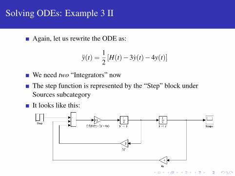
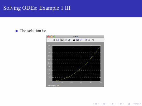
Solving ODEs: Example 3 II
Again, let us rewrite the ODE as:
y(t) =12[H(t)−3y(t)−4y(t)]
We need two “Integrators” now
The step function is represented by the “Step” block underSources subcategory
It looks like this:
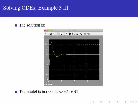
Solving ODEs: Example 3 III
The solution is:
The model is in the file ode3.mdl
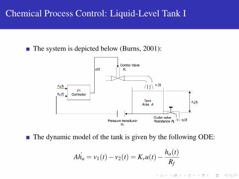
Chemical Process Control: Liquid-Level Tank I
The system is depicted below (Burns, 2001):
The dynamic model of the tank is given by the following ODE:
Aha = v1(t)− v2(t) = Kvu(t)− ha(t)Rf

Chemical Process Control: Liquid-Level Tank II
Taking the Laplace Transform of both sides of the ODE yields:
Ha(s) =Rf
1+ARf sV1(s)
Investigate the time response for a step change in hd(t) from 0 to4m
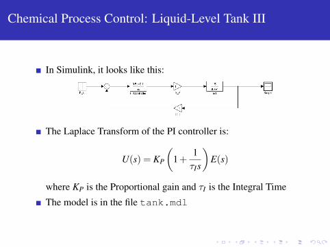
Chemical Process Control: Liquid-Level Tank III
In Simulink, it looks like this:
The Laplace Transform of the PI controller is:
U(s) = KP
(1+
1τIs
)E(s)
where KP is the Proportional gain and τI is the Integral Time
The model is in the file tank.mdl

Chemical Process Control: Non-Isothermal CSTR I
The system is depicted below:

Chemical Process Control: Non-Isothermal CSTR II
The dynamic model of the system is given by the followingODEs:
CA =FV(CAF−CA)− k0 exp
(− Ea
R(T +460)
)CA
T =FV(TF−T)− ∆H
ρCP
[k0 exp
(− Ea
R(T +460)
)CA
]− UAρCPV
(T−Tj)
Controlled Variable: CA
Manipulated Variable: Tj
Load (Disturbance): TF
Given a step disturbance in TF, we wish to control CA bychanging Tj
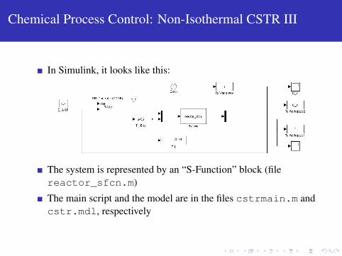
Chemical Process Control: Non-Isothermal CSTR III
In Simulink, it looks like this:
The system is represented by an “S-Function” block (filereactor_sfcn.m)
The main script and the model are in the files cstrmain.m andcstr.mdl, respectively

References
R.S. Burns. Advanced Control Engineering. Butterworth-Heinemann,2001.