Simulations: The Ising Model

Asher Preska Steinberg,∗ Michael Kosowsky, and Seth FradenPhysics Department, Brandeis University, Waltham, MA 02453

(Advanced Physics Lab)(Dated: May 5, 2013)

The goal of this experiment was to create Monte Carlo simulations of the 1D and 2D Ising model.To accomplish this the Metropolis algorithm was implemented in MATLAB. The dependence ofmagnetization on temperature with and without an external field was calculated, as well as thedependence of the energy, specific heat, and magnetic susceptibility on temperature. The results ofthe 2D simulation were compared to the Onsager solution.

I. INTRODUCTION

As technology has improved in the 20th and 21st cen-turies, simulations have become widely used to make pre-dictions about complex systems in a breadth of differentfields, ranging from sports and games to science and engi-neering. For physical scientists, some knowledge of sim-ulations and computing has become essential. Not onlycan simulations help elucidate processes that are diffi-cult to run experiments on in the lab, but they can saveprecious experiment time and money. The focus of thisproject was creating simulations of the Ising model.

A. Properties of Magnetic Materials

This experiment dealt with two types of magnetic ma-terials; ferromagnets and paramagnets. From quantummechanics we know that electrons have there own in-trinsic angular momentum, or spin. Each electron has amagnetic dipole moment (~µ):

~µ = γ~S (1)

. Where γ is the gyromagnetic ratio and ~S is the spin an-gular momentum of the electron [1]. The magnetic prop-erties these materials exhibit are due to the magneticmoments of electrons. When these materials are placed

in a magnetic field ( ~B), the magnetic field exerts a torque

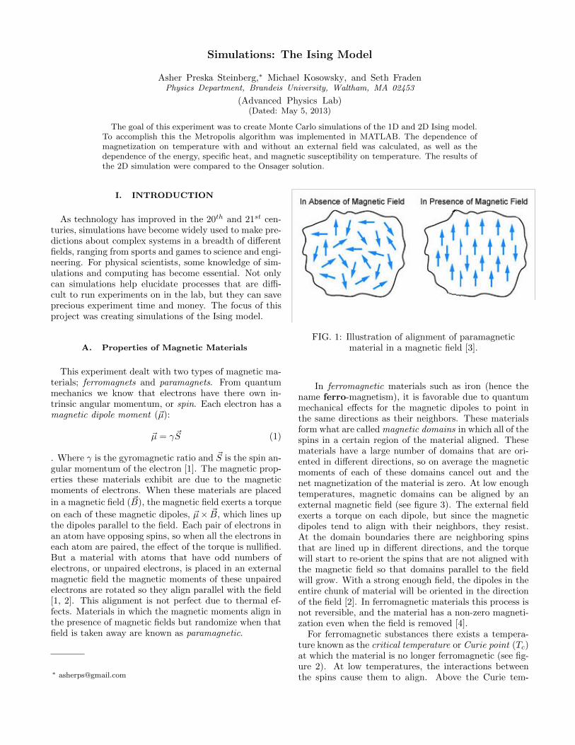
on each of these magnetic dipoles, ~µ× ~B, which lines upthe dipoles parallel to the field. Each pair of electrons inan atom have opposing spins, so when all the electrons ineach atom are paired, the effect of the torque is nullified.But a material with atoms that have odd numbers ofelectrons, or unpaired electrons, is placed in an externalmagnetic field the magnetic moments of these unpairedelectrons are rotated so they align parallel with the field[1, 2]. This alignment is not perfect due to thermal ef-fects. Materials in which the magnetic moments align inthe presence of magnetic fields but randomize when thatfield is taken away are known as paramagnetic.

∗ asherps@gmail.com

FIG. 1: Illustration of alignment of paramagneticmaterial in a magnetic field [3].

In ferromagnetic materials such as iron (hence thename ferro-magnetism), it is favorable due to quantummechanical effects for the magnetic dipoles to point inthe same directions as their neighbors. These materialsform what are called magnetic domains in which all of thespins in a certain region of the material aligned. Thesematerials have a large number of domains that are ori-ented in different directions, so on average the magneticmoments of each of these domains cancel out and thenet magnetization of the material is zero. At low enoughtemperatures, magnetic domains can be aligned by anexternal magnetic field (see figure 3). The external fieldexerts a torque on each dipole, but since the magneticdipoles tend to align with their neighbors, they resist.At the domain boundaries there are neighboring spinsthat are lined up in different directions, and the torquewill start to re-orient the spins that are not aligned withthe magnetic field so that domains parallel to the fieldwill grow. With a strong enough field, the dipoles in theentire chunk of material will be oriented in the directionof the field [2]. In ferromagnetic materials this process isnot reversible, and the material has a non-zero magneti-zation even when the field is removed [4].

For ferromagnetic substances there exists a tempera-ture known as the critical temperature or Curie point (Tc)at which the material is no longer ferromagnetic (see fig-ure 2). At low temperatures, the interactions betweenthe spins cause them to align. Above the Curie tem-

2

FIG. 2: Example of what the phase transition of aferromagnetic material at the Curie point looks like.Vertical axis is magnetization (M/Ms), horizontal is

temperature (T/Tc) [5].

perature, the material undergoes a phase transition andbecomes paramagnetic, with all the magnetic momentsorienting randomly due to thermal effects.

B. The Ising Model

The simplest system that exhibits a phase transition isthe Ising model. Though in this report the Ising modelwill be used to model the phase transition of ferromag-netic materials, this model is broadly applicable. Manypapers are published each year applying the Ising modelto problems in social behavior, neural networks, andother topics. The model was first proposed by WilhemLenz, who gave the problem to his pupil Ernst Ising.Ising solved the model exactly in one dimension, but wasdisappointed to see that there was no phase transition.About 20 years later, Lars Onsager solved the Ising modelexactly in two dimensions in the absence of an externalmagnetic field. The two dimensional model has a phasetransition [4].

In the Ising model, the total energy of the system fora lattice with N spins is given as:

E = −JN∑

i,j=nn(i)

sisj −HN∑i=1

si (2)

The first term represents the spin-spin interaction be-tween a spin and its nearest neighbors. In the Ising modeleach spin (si) is either up or down. In this report, theexchange constant (J) is greater than zero and the ex-ternal magnetic field is in the up direction. The secondterm in eq. 2 represents the energy of a magnetic dipolein a magnetic field, where µ has been incorporated intoH. H will be referred to as the magnetic field [4].

C. Phase Transitions

In the last section it was mentioned that there is nophase transition in the one dimensional Ising model.Why is this? Imagine a simple one dimensional sys-tem of seven spins without an external magnetic field.The ground state of the system is when all the spins arealigned and the energy is E = −7J . Now imagine flippingsome of those spins, creating two domains separated by adomain wall (see figure 4). In this new configuration theenergy of the system is E = −5J . So the energy cost ofcreating one domain wall is 2J . In a one dimensional gridof length N , there are N − 1 different sites this domainwall can be placed, so the change in entropy associatedwith creating one domain wall is ∆S = −kT ln(N − 1).Therefore the free energy cost of creating one domainwall is:

∆F = 2J − kT ln(N − 1) (3)

In one dimension, when the temperature is greater thanzero and as N →∞ the creation of a domain wall alwayslowers the free energy of the system. Since it is favorableto create domain walls when T > 0, more and more do-mains are created until the system is completely random.Therefore in one dimension, the system is paramagneticat all temperatures and there is no phase transition [4].

In two dimensions, for an L× L grid the energy costof creating a domain wall is 2JL (see figure 5). In anL× L grid the domain wall can be placed at L differentcolumns, and the entropy is on the order of lnL. Thefree energy cost of creating one domain wall in two di-mensions is approximately:

∆F ≈ 2JL− kT lnL (4)

In this scenario ∆F > 0 as L → ∞. This means it isnot favorable to create domain walls in two dimensions,and the spins will remain aligned due to the interactionsbetween spins. As mentioned previously, above the criti-cal temperature thermal effects dominate, leading to thesystem becoming disordered. There is therefore a phasetransition in two dimensions.

D. The Metropolis Algorithm

The expectation value of an observable A is given bythe equation:

〈A〉 =

∑iAie

−βEi∑i e−βEi

(5)

Where Ai is the value of the observable for an individualstate (i) [7]. Using equation 5 to calculate observablesis not the most computationally efficient method. Forexample, if one had a simple 10× 10 grid of spins, therewould be 2100 states to sum over. Another method is touse the Metropolis algorithm which is a type of Monte

3

FIG. 3: Alignment of domains when a ferromagnetic material is exposed to an external magnetic field. On the left isan example of unaligned domains. As the magnetic field, H, is turned on, domains aligned in the direction of the

field grow. The spins will remain aligned even after the magnetic field is removed [6].

FIG. 4: The creation of a domain wall in onedimension. Domain wall is indicated in red [4].

FIG. 5: The creation of a domain wall in twodimensions. (a) shows the system with all spins aligned,(b) shows the system after the creation of one domain

wall. Domain wall is indicated by dashed line [4].

Carlo simulation. Monte Carlo simulations are a class ofalgorithms that utilize repeated random sampling to findresults [8].

The Metropolis algorithm works as follows. First, alattice or grid of spins is created. Next, a spin in the gridis chosen at random and the change in energy (∆E) dueto flipping the spin is calculated based on its interactionswith its nearest neighbors (the two nearest neighbors in1D, four nearest in 2D) and the magnetic field (see equa-tion 2). If ∆E < 0 the spin is always flipped. If ∆E > 0then the spin is flipped with a probability (p) determinedby the Boltzmann factor, p = e−β∆E . Following this, avery large number of other random spins are sampled,then the system is sampled even more to account for thetime it takes the system to equilibrate [4].

To get 〈E〉 and 〈E2〉 of the system the energies of eachspin were added up and divided by the total number of

spins. To obtain the average magnetization ,〈M〉, we setµ = 1 and simply summed all the spins (which had valuesof si = ±1) then divided by the total number of spins.Using these quantities, the specific heat (Cv) and mag-netic susceptibility (χ) in a constant magnetic field canbe obtained in terms of the variance of the energy andmagnetization [4, 7, 9, 10]:

Cv =∂〈E〉∂T

= − βT

∂〈E〉∂β

=β

T

∂2 lnZ

∂β2

=β

T

∂

∂β

(1

Z

∂Z

∂β

)

=β

T

(1

Z

∂2Z

∂β2− 1

Z2

(∂Z

∂β

)2)

Cv =β

T(〈E2〉 − 〈E〉2) (6)

Similarly for magnetic susceptibility:

χ =∂〈M〉∂H

= β(〈M2〉 − 〈M〉2) (7)

II. EXPERIMENTAL

A. Basics of Code

The code that we used to carry out these simulationsin two-dimensions is shown in the supplemental materialssection. The programming language that was chosen forthis experiment was MATLAB. Natural units of J/k = 1

4

FIG. 6: Examples of boundary conditions. (a) “Freeends”. The spins on either end are missing one

neighbor. (b) “Periodic” or “torroidal” boundaryconditions. Now the one dimensional array in (a) has

been set up so the spin on the left end of (a) isneighbors with the spin on the right end [4].

were used. Two types of boundary conditions were con-sidered for this project. The first was free ends, in whichthe spins on the edges of the lattice are missing a neigh-bor (see figure 6). The second was periodic or torroidalboundary conditions, in which spins on one edge of thelattice are not only neighbors with the spins directly nextto them, but also with the spins that make up the otheredge of the lattice. For this experiment, periodic bound-ary conditions were chosen. Simulations were run in bothone dimension and two dimensions. In the experiments,two different initial conditions were used. The first wasstarting the simulations where all the spins were alignedrandomly. The second, was where all the spins were ini-tially aligned, as if a magnetic field had been used toalign all the spins before the start of the experiment.

In the code, MATLAB would randomly chose a pointin the lattice and determine the change in energy of flip-ping a spin as ∆E = −2E since s = ±1. As describedin section I D, if ∆E < 0, the spin was always flipped. If∆E > 0, MATLAB would compare the probability deter-mined by the boltzmann factor (p) to a random numberbetween 0 and 1. If the random number was less thanp the spin was flipped. Generally, the grid would berandomly sampled 50 × grid size times, after which themagnetization was measured and the grid would be sam-pled another 50 × grid size times and the magnetizationwas measured again. If the difference between the twomagnetization values was less than 5%, the system wasconsidered equilibrated. If not, the system was sampleduntil the variations in magnetization were under 5%.

III. RESULTS

A. One Dimensional Ising Model

The results for the one dimensional Ising model withH = 0 are shown in figures 7-10. In all of the trialsshown, the initial state of the system at each tempera-

ture was the aligned state (all spins were aligned in samedirection). For the plot of the average energy againsttemperature in figure 7, the basic trend was as expected.As the temperature increased, the energy of the systemslowly began to increase. This was because as the tem-perature was increased, thermal effects become more andmore important and the system wants to go to the mostentropically favorable state. So even though though theenergy due to the spin-spin interactions is increasing, itis still more favorable to the system to go to the mostdisordered state.

Looking at the plot of the average magnetizationagainst temperature (see figure 8) the results are basi-cally what one would expect, with a few exceptions. Attemperatures from around T = 1− 10 the magnetizationof the system is very close to zero. This makes sense be-cause the 1D Ising model is not supposed to have a phasetransition, and the material is supposed to be param-agnetic (see argument in section I C). At temperatureslower than T ≈ 1 though, the magnetization is M ≈ 1, sothere appears to be a phase transition somewhere aroundhere. Since it is well known from Ernst Ising’s solutionthat there should be no phase transition in the 1D Isingmodel, what is causing this?

It turns out that at very low temperatures theMetropolis algorithm fails to give a very physical rep-resentation of the system. The way the Metropolis al-gorithm determines whether or not to flip a spin when∆E > 0 is by comparing a random number to the Boltz-mann factor. But as T → 0 and we have:

limT→0

p = limT→0

e−∆E/kT = 0 (8)

So at temperatures close to zero, the Metropolis algo-rithm will only flip spins so they align, but will neverflip them out of alignment. This is why for very lowtemperatures the magnetization is always 〈M〉 = 1 andalso for extremely low temperatures the energy is alwaysE = −1, which is the energy of the system when all thespins are aligned (see figure 7). The same problem ap-pears when the Metropolis algorithm is used to calculatethe magnetization and energy against temperature in the2D case, but it is less apparent because all the spins aresupposed to remain aligned at low temperatures in the2D case.

In figure 11 the magnetization vs temperature wascompared when H = 0 and H = 1. The results wereas expected. With H = 0, for most of the temperatures(excluding very low temperatures, as explained) the mag-netization is close to 0, since more and more domain wallsare being created until the system is completely random.With H = 1, the spins remain aligned for a larger rangeof temperatures. This is because alignment with the ex-ternal magnetic field lowers the energy of the spins, andthermal effects do not make the system completely ran-dom until the temperature is really increased.

5

FIG. 7: Energy vs temperature for 1D Ising model withH = 0. The grid length was 200 spins, and H = 0. Ateach temperature the system started with all the spins

aligned.

FIG. 8: Magnetization vs temperature for 1D Isingmodel with H = 0. The grid length was 200 spins, andH = 0. At each temperature the system started with all

the spins aligned.

B. Two Dimensional Ising Model

The results for the two dimensional Ising model withH = 0 are shown in figures 12-15. The Onsager solutiongives the critical temperature (Tc) as [4]:

KTcJ

=2

ln(1 +√

2)≈ 2.269 (9)

FIG. 9: Specific heat vs temperature for 1D Ising modelwith H = 0. The grid length was 200 spins, and H = 0.

At each temperature the system started with all thespins aligned.

FIG. 10: Magnetic Susceptibility vs temperature for 1DIsing model with H = 0. The grid length was 200 spins,

and H = 0. At each temperature the system startedwith all the spins aligned.

In our results there is a phase transition from ferromag-netic to paramagnetic somewhere around this tempera-ture. In figure 12, the plot of energy vs temperature, wesee that the energy due to the spin-spin interactions is ata minimum since all the spins are aligned, but somewherearound T = 2−3 there is a sharp rise in energy as the ma-terial switches from ferromagnetic to paramagnetic andthe spins are oriented randomly, raising the energy due tothe spin-spin interactions. In the plot of magnetization

6

FIG. 11: Magnetization vs temperature for 1D Isingmodel with H = 0 and H = 1. The grid length was 200spins. At each temperature the system started with all

the spins aligned.

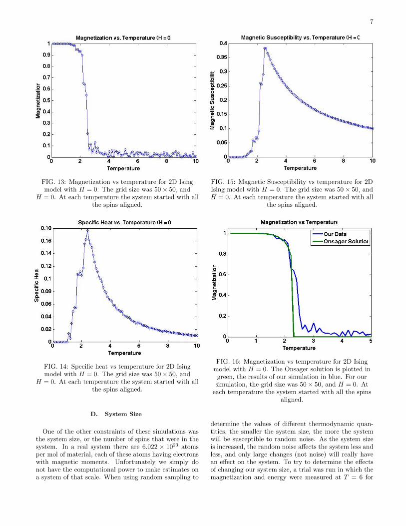
against temperature (fig. 13) a phase transition is alsoobserved. At temperatures below T = 2−3 the spins arealigned and M ≈ 1. For temperatures above T = 2 − 3the spins are randomly oriented and M ≈ 0. The plotsof specific heat and magnetic susceptibility against tem-perature (figures 14 and 15 respectively) show divergentbehavior at the critical temperature as expected. TheOnsager solution for magnetization is given as [11]:

M =

(

1−[sinh log

(1 +√

2)Tc

T

]−4)1/8

T < Tc

0 T > Tc

To compare our results to the Onsager solution, the re-sults for magnetization from our simulation were plottedalong with the above equation in figure 16.

In figure 17 the magnetization vs temperature wascompared when H = 0 and 1. With H = 1, insteadof seeing a sharp transition at the critical temperature ascompared to H = 0, the magnetization instead graduallydecrease to 〈M〉 = 0. This is because like in the one di-mensional case, the energy of each spin is lowered whenthey align with the external magnetic field, so the orderof the system is increased and there is not a sharp tran-sition from an aligned state to the random orientation ofspins. As the temperature is increased to T = 8 − 10,thermal effects dominate, and the net magnetization isclose to zero.

To further examine the effects of applying an externalmagnetic field to the system, a trial was run where thetemperature of the system was fixed at T = 3.5 whilethe magnetic field was increased from H = 0 to 10 (fig-ure 18). Without any external magnetic field, the spinsare all randomly oriented at T = 3.5 (see figure 13) be-

FIG. 12: Energy vs temperature for 2D Ising modelwith H = 0. The grid size was 50× 50, and H = 0. Ateach temperature the system started with all the spins

aligned.

cause T > Tc and thermal effects have randomized thesystem. In figure 18, as the magnitude of the externalmagnetic field is increased, the system goes from a statewhere the spins are oriented randomly to a state wherethe system is completely aligned with the magnetic field.This is because with a strong enough external magneticfield, the aligning torque exerted by the magnetic field(discussed in section I A) is so strong that it overcomesthermal effects and lines up the majority of the magneticdipoles in the direction of the magnetic field.

C. Equilibration of System

As mentioned in section II, the code had a mechanismbuilt in that would keep on sampling until the systemwas considered equilibrated at the temperature, or whenthe magnetization was changing less than 5%. It was im-portant to sample the system sufficiently, because as thesystem was sampled more and more, each individual spinwas more likely to be in its most probable microstate.As more and more spins went to their most probable mi-crostate, the overall system went to its most probablemacrostate or the state the system will be in once itsequilibrated. As the system approaches this state, thefluctuations in the expectation values of thermodynamicquantities begins to decrease, and the decrease in thesefluctuations was used as an indicator that the systemhad reached equilibrium. An example of how the codechecked if the fluctuations had decreased is shown in fig-ure 19.

7

FIG. 13: Magnetization vs temperature for 2D Isingmodel with H = 0. The grid size was 50× 50, and

H = 0. At each temperature the system started with allthe spins aligned.

FIG. 14: Specific heat vs temperature for 2D Isingmodel with H = 0. The grid size was 50× 50, and

H = 0. At each temperature the system started with allthe spins aligned.

D. System Size

One of the other constraints of these simulations wasthe system size, or the number of spins that were in thesystem. In a real system there are 6.022 × 1023 atomsper mol of material, each of these atoms having electronswith magnetic moments. Unfortunately we simply donot have the computational power to make estimates ona system of that scale. When using random sampling to

FIG. 15: Magnetic Susceptibility vs temperature for 2DIsing model with H = 0. The grid size was 50× 50, andH = 0. At each temperature the system started with all

the spins aligned.

FIG. 16: Magnetization vs temperature for 2D Isingmodel with H = 0. The Onsager solution is plotted in

green, the results of our simulation in blue. For oursimulation, the grid size was 50× 50, and H = 0. At

each temperature the system started with all the spinsaligned.

determine the values of different thermodynamic quan-tities, the smaller the system size, the more the systemwill be susceptible to random noise. As the system sizeis increased, the random noise affects the system less andless, and only large changes (not noise) will really havean effect on the system. To try to determine the effectsof changing our system size, a trial was run in which themagnetization and energy were measured at T = 6 for

8

FIG. 17: Magnetization vs temperature for 2D Isingmodel with H = 0 and 1. The grid size was 50× 50. Ateach temperature the system started with all the spins

aligned.

FIG. 18: Magnetization vs magnetic field for twodimensional Ising model with T = 3.5.The grid size was

50× 50, and H = 0. The system started will all thespins aligned.

systems of different sizes (see figures 20 and 21). In bothfigures the fluctuations in the measured values of observ-ables appear to decrease some as the size of the grid isincreased. Since the values of energy and magnetizationare still varying some once the size of the grid that wasused in this experiment is reached, it means that at thissize the results are still subject to some randomness.

FIG. 19: Equilibration of a 50× 50 grid of spins. Thecode checked if the system was equilibrated every

125,000 samples by determining if the magnetization ofthe system had changed by less than 5%. It can be seen

that after the 40th check the systems fluctuations aregetting smaller and then are finally less than 5%.

FIG. 20: Energy at T = 6 calculated for systems ofdifferent sizes. The sizes ranged from 5× 5 to 50× 50.

The system was started with all spins aligned.

IV. IMPROVEMENTS

There were many improvements that could have beenmade to this experiment. The first lesson that wasquickly learned was to run simulations on a small sys-tem to attempt to debug the code before running simu-lations on very large grids. At the suggestion of ProfessorFraden, some of our trials were visualized in MATLAB.

9

FIG. 21: Magnetization at T = 6 calculated for systemsof different sizes. The sizes ranged from 5× 5 to

50× 50. The system was started with all spins aligned.

This was extremely useful in trying to see if the code wascreating a good model of the system. Realizing thesethings sooner could have cut down on the time that wasspent trying to understand if the metropolis algorithmwas being implemented correctly in the code.

If total simulation time was not a concern another twoaspects of the experiment that could have been optimizedare the way that the code checks if the system has equi-librated and the size of the system. Instead of checkingthe system’s magnetization every 125,000 samples (for a50 × 50 grid) and comparing the magnetization at thecurrent checkpoint to the previous one and seeing if thedifference was less than 5%, the deviations in the mag-netization between multiple checkpoints could have beencompared. This would have allowed us to see if the fluc-tuations were really decreasing, or it was simply randomchance that the magnetization between two checkpointschanged very little. Increasing the size of the system that

the simulation was run on would have led to better agree-ment with the Onsager solution, as explained in sectionIII D. Both of these improvements would have meant anincrease in simulation time for each run.

To improve the time it took to simulate the system, adifferent programming language could have been chosenfor the project. A group of graduate students achievedmuch faster run times using Perl.

V. CONCLUSION

In this experiment Monte Carlo simulations were cre-ated of the 1D and 2D Ising model. To do this theMetropolis algorithm was implemented in MATLAB.The dependence of the energy, magnetization, specificheat, and magnetic susceptibility of the system on tem-perature were calculated for the 1D and 2D Ising model.The results of the simulation for magnetization againsttemperature with and without an external magnetic fieldwere compared. Some simple tests were done to try tounderstand the effects of increasing the amount of sam-pling and the system size in Monte Carlo simulations.The experiment was a success in that we learned some ofthe basics of how to run simulations and achieved resultsthat were comparable to the Onsager solution.

VI. CODE

Please see the attached file, 2DIsingModel.m, for asample code that was used in this project.

ACKNOWLEDGMENTS

I would like to thank my lab partner, MichaelKosowsky, for all his help and insight. We would bothlike to thank Andreas Rauch, Sathish Akella and espe-cially Professor Seth Fraden for all their extremely usefulhelp and advice, as well as their patience.

[1] D. J. Griffiths, Introduction to Quantum Mechanics(Pearson Education, Inc., 2005).

[2] D. J. Griffiths, Introduction to Electrodynamics (PearsonEducation, Inc., 2008).

[3] Magnetism, http://electrical.blogspot.com/2012/06/types-of-magnetism.html (2009).

[4] H. Gould and J. Tobochnik, Thermal and StatisticalPhysics (Princeton University Press, 2009).

[5] UCSD, http://magician.ucsd.edu/Essentials/WebBook76x.png (2013).

[6] Wikipedia, https://en.wikipedia.org/wiki/Magnetic domain(2013).

[7] K. A. Dill and S. Bromberg, Molecular DrivingForces: Statistical Thermodynamics in Biology, Chem-istry, Physics, and Nanoscience (Garland Science, Tay-lor & Francis Group, LLC, 2011).

[8] Wikipedia, http://en.wikipedia.org/wiki/Monte Carlo method(2013).

[9] K. Zengel, http://fraden.brandeis.edu/courses/phys39/simulations/Simulation.html (2013).

[10] L. Larrimore, http://fraden.brandeis.edu/courses/phys39/simulations/Simulation.html (2013).

[11] Wikipedia, http://en.wikipedia.org/wiki/Ising model(2013).