Embed Size (px)
Citation preview
Simulations of Supercritical Aerofoil at
Different Angle of Attack With a Simple
Aerofoil using Fluent
1Ravi shankar P R,
Mtech
scholar, Department Mechanical
Engineering,
PDA college of Engineering
Gulbarga, Karnataka, India
2H.
K. Amarnath
Professor, Department of
Mechanical Engineering,
Gogte Institute of Technology,
Belgum, Karnataka, India
3Omprakash D
Hebbal
Professor, Department Mechanical
Engineering,
PDA college of Engneering
Gulbarga, India
Abstract —This In this project flow over supercritical aerofoil
and simple aerofoil is compared at Mach number 0.6
parameters which are observed are pressure drag and strength
of shockwave as they are one of the parameters which are
prominent in transonic speed. These parameters decide the
efficiency of the aerofoil. In this project NACA SC (02) 0714 and
NACA 4412 aerofoil profiles is considered for analysis. Software
tools used are GAMBIT and FLUENT. Gambit is used for
preparing the geometry and meshing and FLUENT is used for
analyzing the flow. Computational fluid dynamics is used
because preparing a model of aerofoil is a lengthy and difficult
process and wind tunnel capable of 0.6 Mach number is not
available and difficult to produce accurate results In
supercritical aerofoil, thickness of an aerofoil near trailing edge
of lower surface is reduced, so that increase in pressure at
lowers surface and helps in lift of an aircraft easily compared to
simple aerofoil. At 15o angle of attack, pressure drag is 12000
Pascal lower in case of supercritical aerofoil compared to simple
aerofoil.
Keywords— Fluent simulation; supercritical aerofoil; pressure
drag; shock waves; Temperature distribution
I. INTRODUCTION
Transonic jet aircrafts fly at speed of 0.8 to 0.9 Mach
number. At these speeds speed of air reaches speed of sound
some were over the wing and compressibility effects start to
show up. The free stream Mach number at which local sonic
velocities develop is called critical Mach number. It is always
better to increase the critical Mach number so that formation
of shockwaves can be delayed. This can be done either by
sweeping the wings but high sweep is not recommended in
passenger aircrafts as there is loss in lift in subsonic speed and
difficulties during constructions. So engineers thought [1] of
developing an aerofoil which can perform this task without
loss in lift and increase in drag. They increased the thickness
of the leading edge and made the upper surface flat so that
there is no formation of strong shockwave and curved trailing
edge lower surface which incr
eases the pressure at lower surface and account’s for lift.
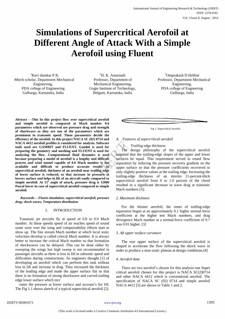
The Fig 1.1 shows sketch of a typical supercritical aerofoil [2].
Fig 1: Supercritical Aerofoil.
A. Features of supercritical aerofoil
1. Trailing edge thickness
The design philosophy of the supercritical aerofoil
required that the trailing-edge slopes of the upper and lower
surfaces be equal. This requirement served to retard flow
separation by reducing the pressure recovery gradient on the
upper surface so that the pressure coefficients recovered to
only slightly positive values at the trailing edge. Increasing the
trailing-edge thickness of an interim 11-percent-thick
supercritical aerofoil from 0 to 1.0 percent of the chord
resulted in a significant decrease in wave drag at transonic
Mach numbers [3];
2. Maximum thickness
For the thinner aerofoil, the onset of trailing-edge
separation began at an approximately 0.1 higher normal-force
coefficient at the higher test Mach numbers, and drag
divergence Mach number at a normal-force coefficient of 0.7
was 0.01 higher. [3]
3. Aft upper surface curvature
The rear upper surface of the supercritical aerofoil is
shaped to accelerate the flow following the shock wave in
order to produce a near-sonic plateau at design conditions.[4]
4. Aerofoil data
There are two aerofoil’s chosen for this analysis one Super
critical aerofoil chosen for this project is NACA SC(2)0714
and other NACA 4412 which is conventional aerofoil. The
specification of NACA SC (02) 0714 and simple aerofoil
NACA 4412 [5] are shown in Table 1 and 2.
International Journal of Engineering Research & Technology (IJERT)
Vol. 3 Issue 8, August - 2014
IJERT
IJERT
ISSN: 2278-0181
www.ijert.orgIJERTV3IS081073
(This work is licensed under a Creative Commons Attribution 4.0 International License.)
1393
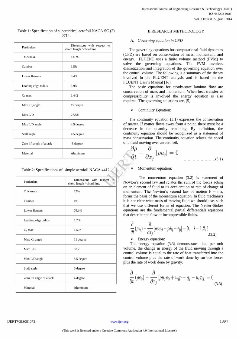
Table 1: Specification of supercritical aerofoil NACA SC (2)
0714.
Particulars Dimensions with respect to
chord length / chord line.
Thickness 13.9%
Camber 1.5%
Lower flatness 9.4%
Leading edge radius 2.9%
CL max 1.442
Max. CL angle 15 degree
Max L/D 27.881
Max L/D angle 4.5 degree
Stall angle 4.5 degree
Zero lift angle of attack -5 degree
Material Aluminum
Table 2: Specifications of simple aerofoil NACA 4412.
Particulars Dimensions with respect to
chord length / chord line.
Thickness 12%
Camber 4%
Lower flatness 76.1%
Leading edge radius 1.7%
CL max 1.507
Max. CL angle 11 degree
Max L/D 57.2
Max L/D angle 5.5 degree
Stall angle 6 degree
Zero lift angle of attack 4 degree
Material Aluminum
II RESEARCH METHODOLOGY
A.
Governing equation in CFD
The governing equations for computational fluid dynamics
(CFD) are based on conservation of mass, momentum, and
energy. FLUENT uses a finite volume method (FVM) to
solve the governing equations. The FVM involves
discretization and integration of the governing equation over
the control volume. The following is a summary of the theory
involved in the FLUENT analysis and is based on the
FLUENT User’s Manual [16].
The basic equations for steady-state laminar flow are
conservation of mass and momentum. When heat transfer or
compressibility is involved the energy equation is also
required. The governing equations are, [5]
Continuity Equation:
The continuity equation (3.1) expresses the conservation
of matter. If matter flows away from a point, there must be a
decrease in the quantity remaining. By definition, the
continuity equation should be recognized as a statement of
mass conservation. The continuity equation relates the speed
of a fluid moving over an aerofoil.
…….………………(3.1)
Momentum equation:
The momentum equation (3.2) is statement of
Newton’s second law and relates the sum of the forces acting
on an element of fluid to its acceleration or rate of change of
momentum. The Newton’s second law of motion F = ma,
forms the basis of the momentum equation. In fluid mechanics
it is not clear what mass of moving fluid we should use, such
that we use different forms of equation. The Navier-Stokes
equations are the fundamental partial differentials equations
that describe the flow of incompressible fluids.
.(3.2)
Energy equation:
The energy equation (3.3) demonstrates that, per unit
volume, the change in energy of the fluid moving through a
control volume is equal to the rate of heat transferred into the
control volume plus the rate of work done by surface forces
plus the rate of work done by gravity.
.(3.3)
International Journal of Engineering Research & Technology (IJERT)
Vol. 3 Issue 8, August - 2014
IJERT
IJERT
ISSN: 2278-0181
www.ijert.orgIJERTV3IS081073
(This work is licensed under a Creative Commons Attribution 4.0 International License.)
1394
2. Approach using FLUENT
The continuity and momentum equations, along with the
realizable k-ε model with pressure gradients effects for
turbulent flows, are solved using the FVM in FLUENT. A
pressure based solver is used since the flow is incompressible
and separation is caused by adverse pressure gradients.
B. Import edge
To specify the aerofoil geometry we will import a file
containing a list of vertices along the surface and have
GAMBIT join these vertices to create edge, corresponding to
the surface of the aerofoil [17]. Fig 2 shows the importing
edges of an aerofoil.
Main Menu >File >Input >ICEM input
Fig 2: Import Edges
C. Crete farfield boundary
We will create the farfield boundary by creating vertices
and joining them appropriately to form edges.
Operation Toolpad >GeometryCommand Button
>Vertex Command Button >Create Vertex
Operation Toolpad >Geometry Command Button >Edge
Command Button >Create Edge
Create edges AB, BC, CD, DA by selecting the vertices
Create Face
We will create the face by selecting the edges AB, BC,
CD, DA naming the face Farfield.
Operation Toolpad > Geometry Command Button >
Face Command Button >Form Face
By selecting the aerofoil edges make an aerofoil face
naming Aerofoil.
Before proceeding to the next step we will subtract the
faces, subtracting face Aerofoil from Farfield.
Operation Toolpad > Geometry Command Button > Face
Command Button
Click on the Boolean Operations Button and select
Subtract Face Box select Farfield
in upper box and Aerofoil in lower box click apply.
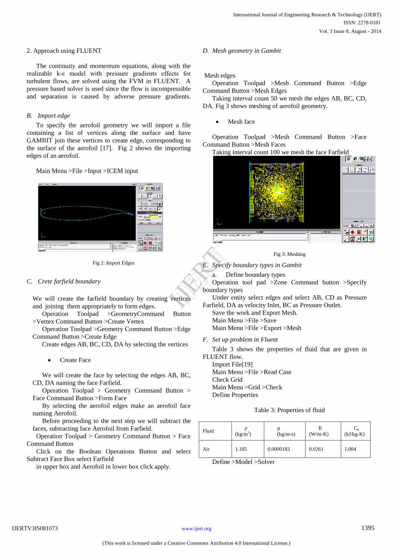
D. Mesh geometry in Gambit
Mesh edges
Operation Toolpad >Mesh Command Button >Edge
Command Button >Mesh Edges
Taking interval count 50 we mesh the edges AB, BC, CD,
DA. Fig 3 shows meshing of aerofoil geometry.
Mesh face
Operation Toolpad >Mesh Command Button >Face
Command Button >Mesh Faces
Taking interval count 100 we mesh the face Farfield
Fig 3: Meshing
E. Specify boundary types in Gambit
a. Define boundary types
Operation tool pad >Zone Command button >Specify
boundary types
Under entity select edges and select AB, CD as Pressure
Farfield, DA as velocity Inlet, BC as Pressure Outlet.
Save the work and Export Mesh.
Main Menu >File >Save
Main Menu >File >Export >Mesh
F. Set up problem in Fluent
Table 3 shows the properties of fluid that are given in
FLUENT flow.
Import File[19]
Main Menu >File >Read Case
Check Grid
Main Menu >Grid >Check
Define Properties
Table 3: Properties of fluid
Fluid ρ
(kg/m3)
µ
(kg/m-s)
K
(W/m-K)
Cp
(kJ/kg-K)
Air 1.185 0.0000183 0.0261 1.004
Define >Model >Solver
International Journal of Engineering Research & Technology (IJERT)
Vol. 3 Issue 8, August - 2014
IJERT
IJERT
ISSN: 2278-0181
www.ijert.orgIJERTV3IS081073
(This work is licensed under a Creative Commons Attribution 4.0 International License.)
1395
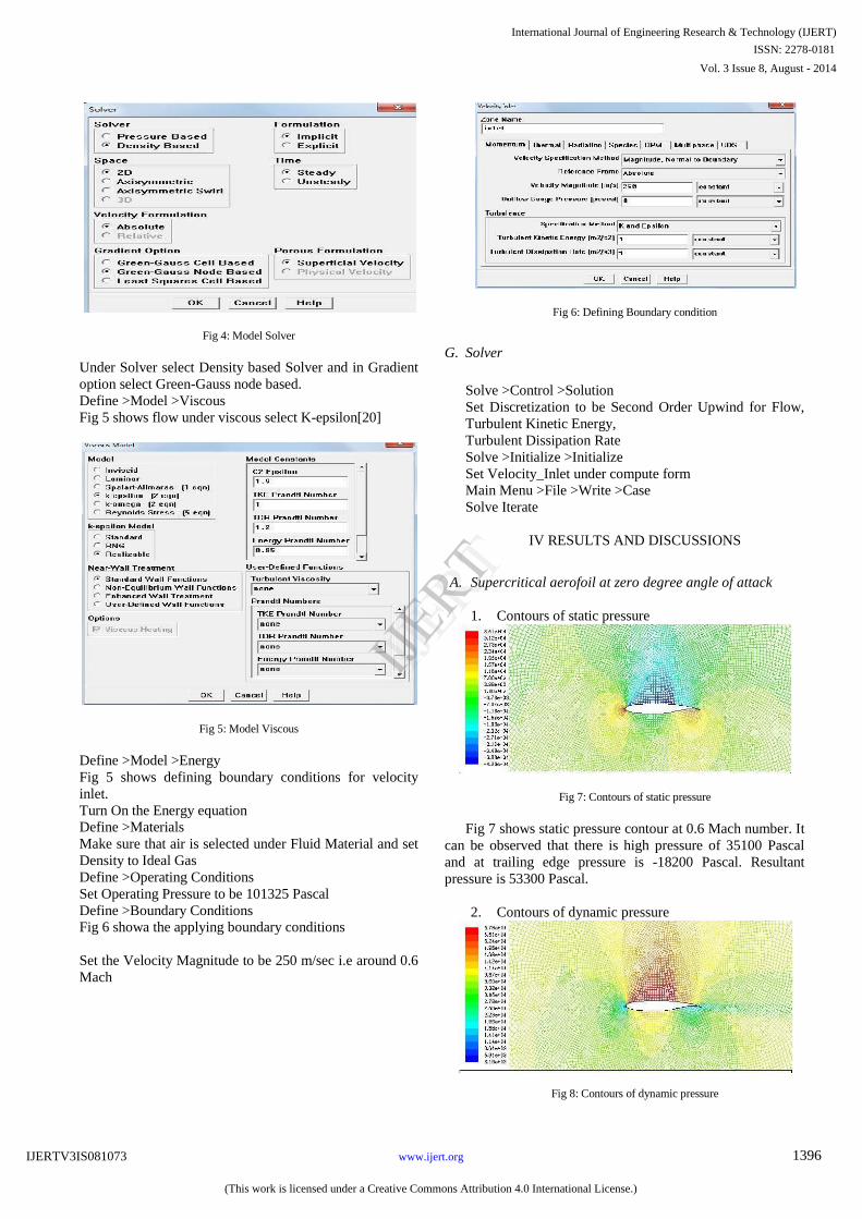
Fig 4: Model Solver
Under Solver select Density based Solver and in Gradient
option select Green-Gauss node based.
Define >Model >Viscous
Fig 5 shows flow under viscous select K-epsilon[20]
Fig 5: Model Viscous
Define >Model >Energy
Fig 5 shows defining boundary conditions for velocity
inlet.
Turn On the Energy equation
Define >Materials
Make sure that air is selected under Fluid Material and set
Density to Ideal Gas
Define >Operating Conditions
Set Operating Pressure to be 101325 Pascal
Define >Boundary Conditions
Fig 6 showa the applying boundary conditions
Set the Velocity Magnitude to be 250 m/sec i.e around 0.6
Mach
Fig 6: Defining Boundary condition
G. Solver
Solve >Control >Solution
Set Discretization to be Second Order Upwind for Flow,
Turbulent Kinetic Energy,
Turbulent Dissipation Rate
Solve >Initialize >Initialize
Set Velocity_Inlet under compute form
Main Menu >File >Write >Case
Solve Iterate
IV RESULTS AND DISCUSSIONS
A. Supercritical aerofoil at zero degree angle of attack
1. Contours of static pressure
Fig 7: Contours of static pressure
Fig 7 shows static pressure contour at 0.6 Mach number. It
can be observed that there is high pressure of 35100 Pascal
and at trailing edge pressure is -18200 Pascal. Resultant
pressure is 53300 Pascal.
2. Contours of dynamic pressure
Fig 8: Contours of dynamic pressure
International Journal of Engineering Research & Technology (IJERT)
Vol. 3 Issue 8, August - 2014
IJERT
IJERT
ISSN: 2278-0181
www.ijert.orgIJERTV3IS081073
(This work is licensed under a Creative Commons Attribution 4.0 International License.)
1396
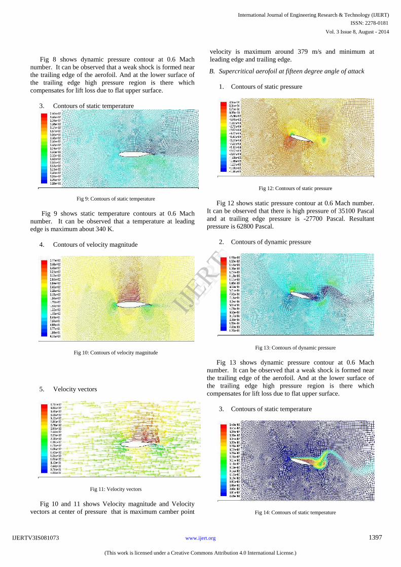
Fig 8 shows dynamic pressure contour at 0.6 Mach
number. It can be observed that a weak shock is formed near
the trailing edge of the aerofoil. And at the lower surface of
the trailing edge high pressure region is there which
compensates for lift loss due to flat upper surface.
3. Contours of static temperature
Fig 9: Contours of static temperature
Fig 9 shows static temperature contours at 0.6 Mach
number. It can be observed that a temperature at leading
edge is maximum about 340 K.
4. Contours of velocity magnitude
Fig 10: Contours of velocity magnitude
5. Velocity vectors
Fig 11: Velocity vectors
Fig 10 and 11 shows Velocity magnitude and Velocity
vectors at center of pressure that is maximum camber point
velocity is maximum around 379 m/s and minimum at
leading edge and trailing edge.
B. Supercritical aerofoil at fifteen degree angle of attack
1. Contours of static pressure
Fig 12: Contours of static pressure
Fig 12 shows static pressure contour at 0.6 Mach number.
It can be observed that there is high pressure of 35100 Pascal
and at trailing edge pressure is -27700 Pascal. Resultant
pressure is 62800 Pascal.
2. Contours of dynamic pressure
Fig 13: Contours of dynamic pressure
Fig 13 shows dynamic pressure contour at 0.6 Mach
number. It can be observed that a weak shock is formed near
the trailing edge of the aerofoil. And at the lower surface of
the trailing edge high pressure region is there which
compensates for lift loss due to flat upper surface.
3. Contours of static temperature
Fig 14: Contours of static temperature
International Journal of Engineering Research & Technology (IJERT)
Vol. 3 Issue 8, August - 2014
IJERT
IJERT
ISSN: 2278-0181
www.ijert.orgIJERTV3IS081073
(This work is licensed under a Creative Commons Attribution 4.0 International License.)
1397
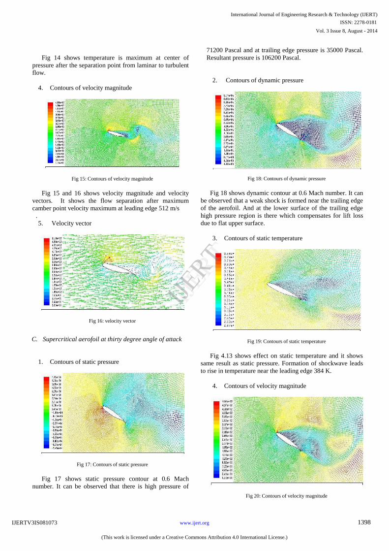
Fig 14 shows temperature is maximum at center of
pressure after the separation point from laminar to turbulent
flow.
4. Contours of velocity magnitude
Fig 15: Contours of velocity magnitude
Fig 15 and 16 shows velocity magnitude and velocity
vectors. It shows the flow separation after maximum
camber point velocity maximum at leading edge 512 m/s
.
5. Velocity vector
Fig 16: velocity vector
C. Supercritical aerofoil at thirty degree angle of attack
1. Contours of static pressure
Fig 17: Contours of static pressure
Fig 17 shows static pressure contour at 0.6 Mach
number. It can be observed that there is high pressure of
71200 Pascal and at trailing edge pressure is 35000 Pascal.
Resultant pressure is 106200 Pascal.
2. Contours of dynamic pressure
Fig 18: Contours of dynamic pressure
Fig 18 shows dynamic contour at 0.6 Mach number. It can
be observed that a weak shock is formed near the trailing edge
of the aerofoil. And at the lower surface of the trailing edge
high pressure region is there which compensates for lift loss
due to flat upper surface.
3. Contours of static temperature
Fig 19: Contours of static temperature
Fig 4.13 shows effect on static temperature and it shows
same result as static pressure. Formation of shockwave leads
to rise in temperature near the leading edge 384 K.
4. Contours of velocity magnitude
Fig 20: Contours of velocity magnitude
International Journal of Engineering Research & Technology (IJERT)
Vol. 3 Issue 8, August - 2014
IJERT
IJERT
ISSN: 2278-0181
www.ijert.orgIJERTV3IS081073
(This work is licensed under a Creative Commons Attribution 4.0 International License.)
1398
5. Velocity vectors
Fig 21: velocity vector
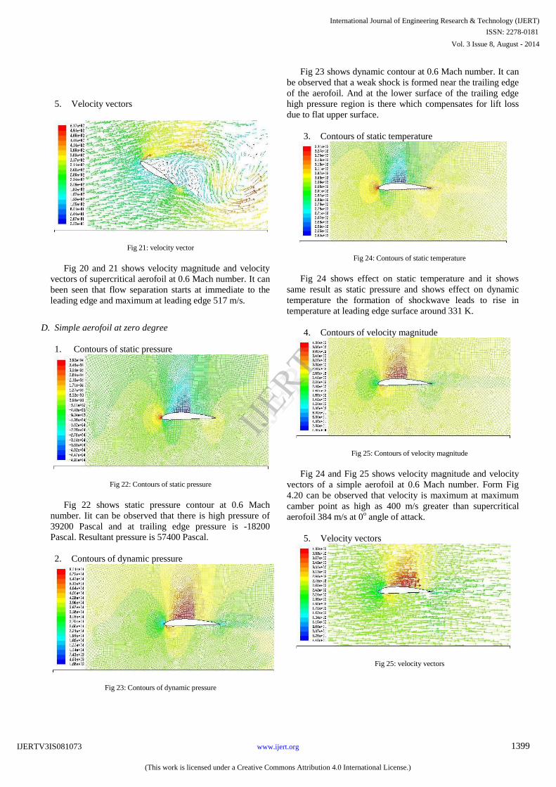
Fig 20 and 21 shows velocity magnitude and velocity
vectors of supercritical aerofoil at 0.6 Mach number. It can
been seen that flow separation starts at immediate to the
leading edge and maximum at leading edge 517 m/s.
D. Simple aerofoil at zero degree
1. Contours of static pressure
Fig 22: Contours of static pressure
Fig 22 shows static pressure contour at 0.6 Mach
number. Iit can be observed that there is high pressure of
39200 Pascal and at trailing edge pressure is -18200
Pascal. Resultant pressure is 57400 Pascal.
2. Contours of dynamic pressure
Fig 23: Contours of dynamic pressure
Fig 23 shows dynamic contour at 0.6 Mach number. It can
be observed that a weak shock is formed near the trailing edge
of the aerofoil. And at the lower surface of the trailing edge
high pressure region is there which compensates for lift loss
due to flat upper surface.
3. Contours of static temperature
Fig 24: Contours of static temperature
Fig 24 shows effect on static temperature and it shows
same result as static pressure and shows effect on dynamic
temperature the formation of shockwave leads to rise in
temperature at leading edge surface around 331 K.
4. Contours of velocity magnitude
Fig 25: Contours of velocity magnitude
Fig 24 and Fig 25 shows velocity magnitude and velocity
vectors of a simple aerofoil at 0.6 Mach number. Form Fig
4.20 can be observed that velocity is maximum at maximum
camber point as high as 400 m/s greater than supercritical
aerofoil 384 m/s at 0o angle of attack.
5. Velocity vectors
Fig 25: velocity vectors
International Journal of Engineering Research & Technology (IJERT)
Vol. 3 Issue 8, August - 2014
IJERT
IJERT
ISSN: 2278-0181
www.ijert.orgIJERTV3IS081073
(This work is licensed under a Creative Commons Attribution 4.0 International License.)
1399
E. Simple aerofoil at fifteen degree
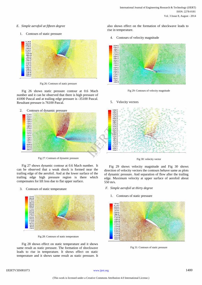
1. Contours of static pressure
Fig 26: Contours of static pressure
Fig 26 shows static pressure contour at 0.6 Mach
number and it can be observed that there is high pressure of
41000 Pascal and at trailing edge pressure is -35100 Pascal.
Resultant pressure is 76100 Pascal.
2. Contours of dynamic pressure
Fig 27: Contours of dynamic pressure
Fig 27 shows dynamic contour at 0.6 Mach number. It
can be observed that a weak shock is formed near the
trailing edge of the aerofoil. And at the lower surface of the
trailing edge high pressure region is there which
compensates for lift loss due to flat upper surface.
3. Contours of static temperature
Fig 28: Contours of static temperature
Fig 28 shows effect on static temperature and it shows
same result as static pressure. The formation of shockwave
leads to rise in temperature. It shows effect on static
temperature and it shows same result as static pressure. It
also shows effect on the formation of shockwave leads to
rise in temperature.
4. Contours of velocity magnitude
Fig 29: Contours of velocity magnitude
5. Velocity vectors
Fig 30: velocity vector
Fig 29 shows velocity magnitude and Fig 30 shows
direction of velocity vectors the contours behave same as plots
of dynamic pressure. And separation of flow after the trailing
edge. Maximum velocity at upper surface of aerofoil about
550 m/s.
F. Simple aerofoil at thirty degree
1. Contours of static pressure
Fig 31: Contours of static pressure
International Journal of Engineering Research & Technology (IJERT)
Vol. 3 Issue 8, August - 2014
IJERT
IJERT
ISSN: 2278-0181
www.ijert.orgIJERTV3IS081073
(This work is licensed under a Creative Commons Attribution 4.0 International License.)
1400
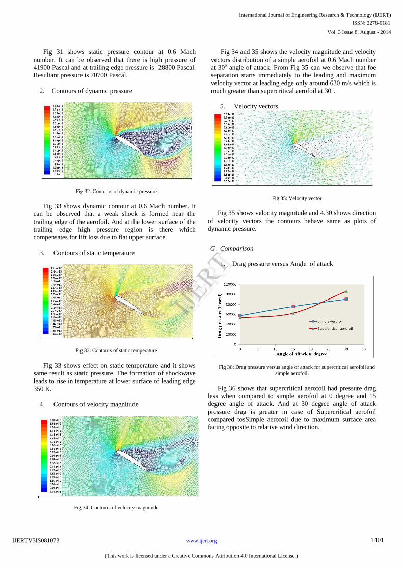
Fig 31 shows static pressure contour at 0.6 Mach
number. It can be observed that there is high pressure of
41900 Pascal and at trailing edge pressure is -28800 Pascal.
Resultant pressure is 70700 Pascal.
2. Contours of dynamic pressure
Fig 32: Contours of dynamic pressure
Fig 33 shows dynamic contour at 0.6 Mach number. It
can be observed that a weak shock is formed near the
trailing edge of the aerofoil. And at the lower surface of the
trailing edge high pressure region is there which
compensates for lift loss due to flat upper surface.
3. Contours of static temperature
Fig 33: Contours of static temperature
Fig 33 shows effect on static temperature and it shows
same result as static pressure. The formation of shockwave
leads to rise in temperature at lower surface of leading edge
350 K.
4. Contours of velocity magnitude
Fig 34: Contours of velocity magnitude
Fig 34 and 35 shows the velocity magnitude and velocity
vectors distribution of a simple aerofoil at 0.6 Mach number
at 30o angle of attack. From Fig 35 can we observe that foe
separation starts immediately to the leading and maximum
velocity vector at leading edge only around 630 m/s which is
much greater than supercritical aerofoil at 30o.
5. Velocity vectors
Fig 35: Velocity vector
Fig 35 shows velocity magnitude and 4.30 shows direction
of velocity vectors the contours behave same as plots of
dynamic pressure.
G. Comparison
1. Drag pressure versus Angle of attack
Fig 36: Drag pressure versus angle of attack for supercritical aerofoil and
simple aerofoil.
Fig 36 shows that supercritical aerofoil had pressure drag
less when compared to simple aerofoil at 0 degree and 15
degree angle of attack. And at 30 degree angle of attack
pressure drag is greater in case of Supercritical aerofoil
compared tosSimple aerofoil due to maximum surface area
facing opposite to relative wind direction.
International Journal of Engineering Research & Technology (IJERT)
Vol. 3 Issue 8, August - 2014
IJERT
IJERT
ISSN: 2278-0181
www.ijert.orgIJERTV3IS081073
(This work is licensed under a Creative Commons Attribution 4.0 International License.)
1401
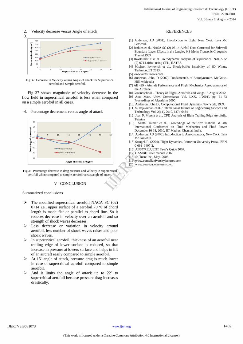
2. Velocity decrease versus Angle of attack
3.
Fig 37: Decrease in Velocity versus Angle of attack for Supercritical aerofoil and Simple aerofoil.
Fig 37 shows magnitude of velocity decrease in the
flow field in supercritical aerofoil is less when compared
on a simple aerofoil in all cases.
4. Percentage decrement versus angle of attack
Fig 38: Percentage decrease in drag pressure and velocity in supercritical
aerofoil when compared to simple aerofoil versus angle of attack.
V CONCLUSION
Summarized conclusions
The modified supercritical aerofoil NACA SC (02)
0714 i.e., upper surface of a aerofoil 70 % of chord
length is made flat or parallel to chord line. So it
reduces decrease in velocity over an aerofoil and so
strength of shock waves decreases.
Less decrease or variation in velocity around
aerofoil, less number of shock waves raises and poor
shock waves.
In supercritical aerofoil, thickness of an aerofoil near
trailing edge of lower surface is reduced, so that
increase in pressure at lowers surface and helps in lift
of an aircraft easily compared to simple aerofoil.
At 15o angle of attack, pressure drag is much lower
in case of supercritical aerofoil compared to simple
aerofoil.
And it limits the angle of attack up to 22o to
supercritical aerofoil because pressure drag increases
drastically.
REFERENCES
[1] Anderson, J.D (2001), Introduction to flight, New York, Tata Mc
Grawhill.
[2] Jenkins et al., NASA SC (2)-07 14 Airfoil Data Corrected for Sidewall
Boundary-Layer Effects in the Langley 0.3-Meter Transonic Cryogenic Tunnel,1989
[3] Ravikumar T et al., Aerodynamic analysis of supercritical NACA sc
(2)-0714 airfoil using CFD, IJATES. [4] Michael Iovnovich et al., Shock-buffet Instability of 3D Wings,
Technion, IIT 2013.
[5] www.airfoilstools.com. [6] Anderson, John, D (2007). Fundamentals of Aerodynamics. McGraw-
Hill, wikipedia
[7] AE 429 - Aircraft Performance and Flight Mechanics Aerodynamics of the Airplane.
[8] Groundschool – Theory of Flight- Aerofoils and wings 18 August 2012
[9] Acta Math. Univ. Comenianae Vol. LXX, 1(2001), pp. 51–73
Proceedings of Algorithm 2000
[10] Anderson, John D., Computational Fluid Dynamics New York, 1989.
[11] S. Rajakumar. et.al. / International Journal of Engineering Science and Technology Vol. 2(11), 2010, 6474-6484
[12] Juan P. Murcia et al., CFD Analysis of Blunt Trailing Edge Aerofoils.
Tecnica [13] Senthil kumar et al., Proceedings of the 37th National & 4th
International Conference on Fluid Mechanics and Fluid Power December 16-18, 2010, IIT Madras, Chennai, India.
[14] Anderson, J.D (2005), Introduction to Aerodynamics, New York, Tata
Mc Grawhill. [15] Stengel, R. (2004), Flight Dynamics, Princeton University Press, ISBN
0-691- 1407-2.
[16] ANSYS FLUENT User’s Guide 2009. [17] GAMBIT User manual 2007.
[18] © Fluent Inc., May- 2003
[19] www.cornelluniversitylectures.com [20] www.aerospacelectures.co.cc
International Journal of Engineering Research & Technology (IJERT)
Vol. 3 Issue 8, August - 2014
IJERT
IJERT
ISSN: 2278-0181
www.ijert.orgIJERTV3IS081073
(This work is licensed under a Creative Commons Attribution 4.0 International License.)
1402


![& Aeros ournal of Aeronautics Aerospace Engineering€¦ · 218airfoil: According to airfoil database [13], scatter drawing of an aerofoil in this problem was a 6-digit NACA series,](https://img.pdfslide.us/doc/110x75/5ea7c3f1fa75f029b26137af/-aeros-ournal-of-aeronautics-aerospace-engineering-218airfoil-according-to.jpg)
![A COMPARATIVE FLOW ANALYSIS OF NACA 6409 AND NACA … · aerofoil sections using passive air-jet vortex generators were investigated by Prince et al. [11] Shih et al. [12] showed](https://img.pdfslide.us/doc/110x75/5f9b7d0b7fee8d1057083d28/a-comparative-flow-analysis-of-naca-6409-and-naca-aerofoil-sections-using-passive.jpg)