Simulations of Dynamics and Transport during the September 2002 Antarctic Major Warming

Simulations of Dynamics and Transport during the September 2002 AntarcticMajor Warming

GLORIA L. MANNEY,* JOSEPH L. SABUTIS,� DOUGLAS R. ALLEN,# WILLIAM A. LAHOZ,@

ADAM A. SCAIFE,& CORA E. RANDALL,** STEVEN PAWSON,�� BARBARA NAUJOKAT,##

AND RICHARD SWINBANK&

*Jet Propulsion Laboratory, California Institute of Technology, Pasadena, California, and Department of Natural Sciences,New Mexico Highlands University, Las Vegas, New Mexico

�School of Education and Department of Mathematical Sciences, New Mexico Highlands University, Las Vegas, New Mexico#Remote Sensing Division, Naval Research Laboratory, Washington, D.C.

@Data Assimilation Research Centre, Department of Meteorology, University of Reading, Reading, United Kingdom&Met Office, Exeter, Devon, United Kingdom

**Laboratory for Atmospheric and Space Physics, University of Colorado, Boulder, Colorado��NASA/Goddard Space Flight Center, Greenbelt, and Goddard Earth Science and Technology Center, University of Maryland,

Baltimore County, Baltimore, Maryland##Institut für Meteorologie, Freie Universität Berlin, Berlin, Germany

(Manuscript received 19 May 2003, in final form 21 January 2004)

ABSTRACT

A mechanistic model simulation initialized on 14 September 2002, forced by 100-hPa geopotential heightsfrom Met Office analyses, reproduced the dynamical features of the 2002 Antarctic major warming. Thevortex split on �25 September; recovery after the warming, westward and equatorward tilting vortices, andstrong baroclinic zones in temperature associated with a dipole pattern of upward and downward verticalvelocities were all captured in the simulation. Model results and analyses show a pattern of strong upwardwave propagation throughout the warming, with zonal wind deceleration throughout the stratosphere athigh latitudes before the vortex split, continuing in the middle and upper stratosphere and spreading tolower latitudes after the split. Three-dimensional Eliassen–Palm fluxes show the largest upward and pole-ward wave propagation in the 0°–90°E sector prior to the vortex split (coincident with the location ofstrongest cyclogenesis at the model’s lower boundary), with an additional region of strong upward propa-gation developing near 180°–270°E. These characteristics are similar to those of Arctic wave-2 majorwarmings, except that during this warming, the vortex did not split below �600 K. The effects of polewardtransport and mixing dominate modeled trace gas evolution through most of the mid- to high-latitudestratosphere, with a core region in the lower-stratospheric vortex where enhanced descent dominates andthe vortex remains isolated. Strongly tilted vortices led to low-latitude air overlying vortex air, resulting inhighly unusual trace gas profiles. Simulations driven with several meteorological datasets reproduced themajor warming, but in others, stronger latitudinal gradients at high latitudes at the model boundary resultedin simulations without a complete vortex split in the midstratosphere. Numerous tests indicate very highsensitivity to the boundary fields, especially the wave-2 amplitude. Major warmings occurred for initialfields with stronger winds and larger vortices, but not smaller vortices, consistent with the initiation of winddeceleration by upward-propagating waves near the poleward edge of the region where wave 2 can propa-gate above the jet core. Thus, given the observed 100-hPa boundary forcing, stratospheric preconditioningis not needed to reproduce a major warming similar to that observed. The anomalously strong forcing in thelower stratosphere can be viewed as the primary direct cause of the major warming.

1. Introduction

Stratospheric major warmings (wherein the usuallystrong westerlies of the polar night jet are reversed toeasterlies and high latitude temperature gradients re-

verse) are the most dramatic events affecting the win-tertime circulation and transport in the Northern Hemi-sphere (NH). Historically, such warmings have oc-curred in approximately half of NH winters (e.g.,Labitzke 1977, 1982; Naujokat et al. 2002), except dur-ing the unusually cold period in the 1989/1990 through1997/1998 winters (Manney et al. 1999). Because of thetypically much lower temperatures and stronger polarvortex in the Southern Hemisphere (SH), the occur-rence of the first observed major warming in the Ant-

Corresponding author address: Dr. Gloria L. Manney, Depart-ment of Natural Sciences, New Mexico Highlands University, LasVegas, NM 87701.E-mail: [email protected]

690 J O U R N A L O F T H E A T M O S P H E R I C S C I E N C E S VOLUME 62

© 2005 American Meteorological Society

JAS3313

arctic in mid–late September 2002 (e.g., Varotsos 2002;Baldwin et al. 2003; Allen et al. 2003; Weber et al. 2003)was completely unanticipated. As shown by, for ex-ample, Allen et al. (2003), Newman and Nash (2005),and Scaife et al. (2005), the 2002 SH winter strato-sphere was unusually disturbed beginning in May. Sev-eral minor warmings occurred in August and Septem-ber, culminating in a major warming beginning in mid-September that strongly resembled what are commonlyreferred to as “wave-2” warmings (in which the mid-stratospheric polar vortex splits) in the NH (e.g., Allenet al. 2003). The major warming was immediately pre-ceded by an extraordinarily strong (much stronger thantypically observed during NH major warmings) pulse ofeddy heat flux in the lower stratosphere/upper tropo-sphere, indicating unusual upward planetary-scale wavepropagation (e.g., Allen et al. 2003; Sinnhuber et al.2003; Newman and Nash 2005; Scaife et al. 2005).

Mechanistic model simulations have been instrumen-tal in helping to understand the dynamics of strato-spheric sudden warmings. Butchart et al. (1982) wereamong the first to use a detailed primitive equationmodel to test sensitivity of simulations to realistic initialand boundary conditions. Smith (1992) used a mecha-nistic model to explore sensitivity of major warmingoccurrence to initial and boundary fields from varioustimes. Manney et al. (1994a) compared simulations ofthe February 1979 major warming using isentropic andpressure coordinate models and examined sensitivity toinitial date, forcing datasets, radiation scheme, andmodel resolution. Jung et al. (2001) used an isentropicvertical coordinate model and boundary sensitivity teststo examine the role of various mechanisms in the re-covery phase of the February 1979 major warming.These studies helped elucidate characteristics of bound-ary and initial conditions important to simulating majorwarmings, and hence shed light on the mechanisms in-volved in producing such warmings. Simulations of ma-jor warmings have also been used to study developmentof small-scale structure (e.g., Fairlie et al. 1990a; Man-ney et al. 1994a) and details of air motion and tracertransport (e.g., Manney et al. 1994a, 2000a), topics forwhich observation-based datasets are often too incom-plete, sparse, or of too coarse resolution to study indetail.

Several studies have used more idealized simulationsto examine aspects of the NH stratospheric circulationand the conditions under which major warmings occur.O’Neill and Pope (1988) used mechanistic model simu-lations to contrast the response of the stratosphere toweak and strong boundary level forcing, showing theimportance of nonlinear effects in the strong forcingregimes under which major warmings may occur, andarguing against the relevance of the “preconditioning”concept as applied to the occurrence of major warm-ings. Scott and Haynes (1998) showed that interannualvariability, including stratospheric warmings, arosefrom internal variability under certain ranges of bound-

ary forcing and argued that zonal flow anomalies in thesubtropics were responsible for this variability. Scaifeand James (2000) showed weak, moderate, and strongforcing regimes in the NH winter, leading to strongwesterly flow, unsteady westerly flow, and oscillationsbetween westerly and easterly flow, respectively. Grayet al. (2003) used a mechanistic model with an ensembleapproach to investigate the response of the NH strato-spheric flow regime to changes in tropospheric waveforcing and equatorial wind direction. They found thatmajor warmings always occurred with strong forcingand never occurred with weak forcing, but in an inter-mediate forcing regime, tropospheric forcing was lesscritical, and other factors such as early-winter initialconditions and the quasi-biennial oscillation (QBO)phase influenced the occurrence of major warmings.

Here we have used the U.K. Universities Global At-mospheric Modeling Project (UGAMP) Stratosphere–Mesosphere Model (USMM) to simulate the SH 2002stratospheric major warming. Having obtained a veryrealistic simulation of the event, we use the observa-tions and simulations to examine aspects of the dynam-ics of the warming and modeled long-lived tracers togive an overview of transport. Sensitivity tests tochanges in initialization and boundary forcing are usedto elucidate some of the important features of thestratospheric flow conditions that allowed this unprec-edented warming to occur.

2. Model and data description

a. USMM model description

The USMM (Thuburn and Brugge 1994) is a spectral,primitive equation model of the stratosphere and me-sosphere forced at the lower boundary by specified geo-potential height fields. The configuration of the USMMused here is the same as that described by Manney et al.(2002). It has 34 isobaric levels from 89.5 to 0.01 hPa(MacKenzie et al. 1999; vertical resolution of �1.6 km),a lower boundary at 100 hPa, an upper boundary con-dition of no mass flux through zero pressure, and atruncation at T42 (horizontal resolution �3°). Themodel has extra scale-selective diffusion in the meso-sphere, which, with the short radiative time scalesthere, helps to damp waves and reduce the possibility ofwave reflection at the boundary.

Gravity wave drag is parameterized by applying asimple Rayleigh friction with an altitude-dependentdamping coefficient (damping times range from 116days at and below 50 km to 1.4 days at 80 km) to thezonal wind (Thuburn and Brugge 1994; MacKenzie etal. 1999). While the USMM can be run with a nonoro-graphic gravity wave scheme, the selection of gravitywave characteristics is problematic and largely arbitrary(e.g., Manney et al. 2002), and the model has previouslybeen used successfully to simulate major warmingswithout including this scheme (Manney et al. 1999).

MARCH 2005 M A N N E Y E T A L . 691

The USMM uses the middle atmosphere radiationcode (MIDRAD) first described by Shine (1987), withseasonally and meridionally varying upwelling fluxes ofIR radiation in the 9.6- and 15-�m wavelength regionscalculated using climatological temperatures, assumingthat emission at 9.6 �m originates at 700 hPa and emis-sion at 15 �m originates at 130 hPa. A prescribed, zonalmean climatological ozone field is used in the radiationcalculations. The USMM’s online transport calculationis described by Thuburn and Brugge (1994); a standardspectral scheme is used in the horizontal, with a flux-limited scheme in the vertical.

b. Initialization and boundary fields

For most of the results shown here, the model wasforced at 100 hPa using daily geopotential heights fromthe Met Office’s stratosphere–troposphere assimilationsystem (Swinbank and O’Neill 1994; Swinbank et al.2002) and initialized using Met Office three-dimensional (3D) wind and temperature fields. Met Of-fice winds and temperatures above their top level of 0.3hPa are extrapolated up to the top USMM level usingthermal wind balance in the zonal mean. Sensitivitytests to initialization date and configuration of initialand boundary fields are all done using the Met Officedata. The sensitivity of the model simulations to thedataset used for initialization and forcing is tested insimulations using data from the National Centers forEnvironmental Prediction (NCEP) Climate PredictionCenter (CPC), the European Centre for Medium-Range Weather Forecasts (ECMWF), and the NationalAeronautics and Space Administration (NASA) God-dard Earth Observation System, versions 3 and 4(GEOS-3 and -4) assimilation systems. These comprisethe most commonly used gridded meteorologicaldatasets that cover the stratosphere. Except for GEOS-4, the main features of these datasets are described byManney et al. (2003). The high-resolution GEOS andECMWF data have been interpolated to 2° � 2.5° and2.5° � 2.5° grids, respectively. The ECMWF data arefrom the operational assimilations for SH 2002 (seeSimmons et al. 2005). The GEOS-4 data use the Physi-cal Space Statistical Analysis Scheme (Cohn et al.1998), as in GEOS-3, but with a new model (Lin 2004);see Schoeberl et al. (2003) and Douglass et al. (2003)for further details.

Four chemical tracers and several idealized tracerswere included in the model simulations. Idealized trac-ers are initialized with potential vorticity (PV), latitude,log10(pressure), log(potential temperature �), andequivalent latitude [EqL, the latitude equivalent to thearea enclosed by each PV contour; similar to the “tracerequivalent latitude” used by Allen et al. (2003), andreferences therein, with small vertical gradients, so itemphasizes horizontal motions]. Methane (CH4), watervapor (H2O), nitrous oxide (N2O), and ozone (O3) areinitialized with 3D fields reconstructed from EqL/�-space mappings of Upper Atmosphere Research Satellite

(UARS) long-lived trace gas data from a “climatology”based on Cryogenic Limb Array Etalon SpectrometerCH4 and N2O and Microwave Limb Sounder H2O andO3, from April 1992 through March 1993 (e.g., Manneyet al. 2000b). The UARS CH4, N2O, and H2O fieldsused here are not reliable below 68 hPa (or in somecases, lower pressure in low latitudes), so the initializa-tion fields contain some artifacts that can produce un-realistic results in the lowest levels. The idealized trac-ers that isolate vertical motion [the log(�) andlog10(pressure) tracers] show clearly that the model’svertical transport is not realistic in the lowest levels;thus, quantitative estimates of diabatic descent fromthe tracer fields are not attempted below �550 K.

The control simulation was initialized on 14 Septem-ber 2002 and forced using Met Office 100-hPa geopo-tential heights. This initialization date was chosen asone with a lull in wave activity at 100 hPa prior to thedevelopment of the warming. Other simulations testthe sensitivity to initialization date, initial fields, andboundary forcing. Boundary fields are provided to themodel once daily at 1200 UTC. For sensitivity tests inwhich the boundary or initial fields are altered so thatthey may be dynamically inconsistent, the boundaryfields are relaxed from the initial day’s 100-hPa geopo-tential heights to the desired value over the first 3 days.

Potential vorticity (and horizontal winds from theNCEP CPC analyses) is calculated from the meteoro-logical analyses (Newman et al. 1989; Manney et al.1996) for comparison with PV from the USMM simu-lations, which is an output of the USMM’s postprocess-ing program and is thus calculated using a differentalgorithm; there is therefore sometimes a bias betweenthe two fields. Eliassen–Palm (EP) fluxes (e.g., An-drews et al. 1987, and references therein) and indices ofrefraction (e.g., Matsuno 1970), which provide mea-sures of wave propagation, and 3D EP fluxes (Plumb1985) are calculated as described by Sabutis (1997) andSabutis et al. (1997), respectively.

3. Modeling dynamical evolution during theSH 2002 major warming

a. Synoptic evolution

Our first simulation of the SH 2002 major warmingwas initialized on 14 September 2002. This initializationdate was chosen during a relative minimum in wave-2activity at 100 hPa, the model’s lower boundary. Figure1 shows the boundary field (Met Office 100-hPa geo-potential heights) in the days leading up to the vortexsplit. There is strong and persistent cyclogenesis(trough formation) in the 0°–90°E sector and weakerand more sporadic cyclogenesis near 270°E; this ismanifested in a wavenumber decomposition as a largeamplification of wave 2 in the boundary forcing. Thestronger anticyclone in the midstratosphere formsdownstream of the region of strongest cyclogenesis,


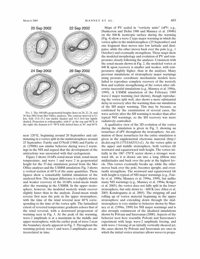
near 120°E, beginning around 20 September and cul-minating in a vortex split in the midstratosphere around25 September. Fairlie and O’Neill (1988) and Fairlie etal. (1990b) saw similar behavior during wave-2 warm-ings in the NH and argued that the development of theanticyclone was associated with that cyclogenesis.

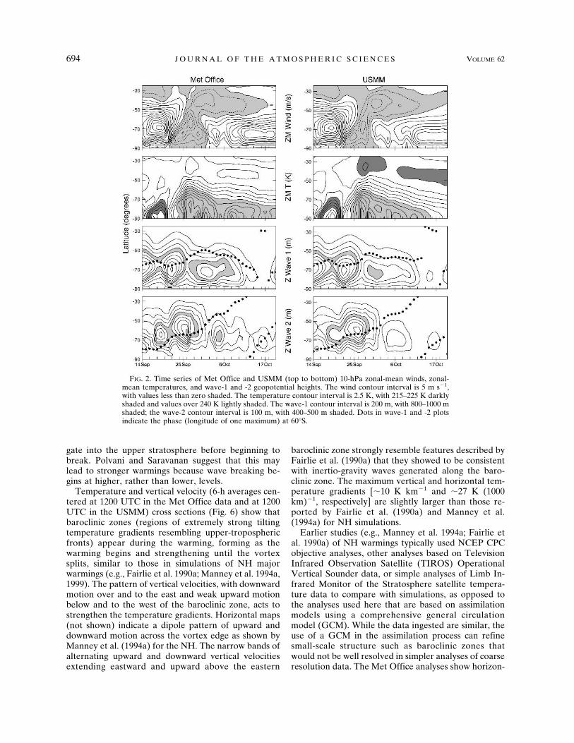
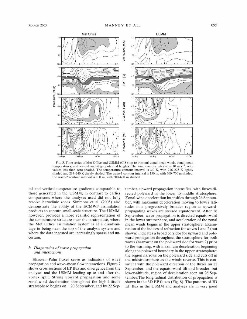
Figure 2 shows 10-hPa zonal-mean wind, zonal-meantemperature, and wave 1 and wave 2 in geopotentialheight for the 37-day simulation period from the MetOffice analyses and the USMM simulation; Fig. 3 showsa vertical section at 60°S of the same quantities. Thesefigures show a remarkably faithful simulation of theanalyzed flow. The largest difference is a slightly slowerand weaker recovery of the 10-hPa zonal-mean windsafter the warming in the USMM. In the upper strato-sphere, however, the modeled westerly winds recoverslightly faster than in the analysis. Zonal-mean windsreverse first near the pole in the upper stratosphere,with the time of the wind reversal near 60°S corre-sponding to the time of the vortex split. The latitudinalextent of reversed temperature gradients echoes that ofthe wind reversal, with a downward progression ofwarming seen in Fig. 3. At the peak of the warming,wave-2 amplitude is at a maximum in the middle andupper stratosphere, with the earlier peak of wave 2 nearthe boundary clearly apparent in Fig. 3. Throughout thewarming period, wave-1 and wave-2 amplitudes are an-ticorrelated in time.

Maps of PV scaled in “vorticity units” (sPV; e.g.,Dunkerton and Delisi 1986 and Manney et al. 1994b)on the 840-K isentropic surface during the warming(Fig. 4) show a wave-2 type major warming in which thevortex splits in the midstratosphere (25 September) andone fragment then moves into low latitude and dissi-pates, while the other moves back over the pole (e.g., 1October) and eventually strengthens. These maps showthe modeled morphology and evolution of PV and tem-perature closely following the analyses. Consistent withthe zonal means shown in Fig. 2, the modeled vortex at840 K upon recovery is smaller and weaker, with tem-peratures slightly higher, than in the analyses. Manyprevious simulations of stratospheric major warmingsusing pressure coordinate mechanistic models havefailed to reproduce complete recovery of the westerlyflow and realistic strengthening of the vortex after oth-erwise successful simulations (e.g., Manney et al. 1994a,1999). A USMM simulation of the February 1989wave-2 major warming (not shown), though reproduc-ing the vortex split well, also shows a more substantialdelay in recovery after the warming than our simulationof the SH major warming. This may be because, asconfirmed by the examination of several cases, thewave activity after the SH warming is weaker than aftertypical NH warmings, so the SH recovery was moreradiatively controlled.

A qualitative view of the 3D evolution of the vortexduring the simulation is given in Fig. 5, showing anisosurface of sPV throughout the stratosphere. An ani-mation of these isosurfaces for the entire simulation isgiven in the supplemental electronic material (http://dx.doi.org/10.1175/JAS3313.s1). As the vortex splits inthe upper and middle stratosphere, both vortices tiltwestward and equatorward with height. The vortex ini-tially in the 180°–270°E sector shows a stronger west-ward tilt, as it is drawn out into a long ribbon intomidlatitudes and back over the pole at the highest lev-els. This vortex eventually breaks up, while the othermoves back over the pole, becomes upright, and even-tually strengthens. The westward and equatorward tiltwith height is typical of NH major warmings (e.g., Fair-lie et al. 1990a; Manney et al. 1994a, 1999), but unlikemany NH warmings (e.g., Manney et al. 1994a; Krügeret al. 2005), the vortex does not fully split in the lowerstratosphere, but only down to �600 K (see Allen et al.2003; Kondragunta et al. 2005). The stripping off androlling up of vortex material beginning in the upperstratosphere and extending down through the mid-stratosphere is very similar to behavior shown by Man-ney et al. (1994a, 1999) for NH major warmings and isalso strongly reminiscent of the idealized simulationsshown by Polvani and Saravanan (2000). Aspects of thebehavior seen here resemble Polvani and Saravanan’sexperiment with large wave-2 amplitude forcing, andwith wave-1 forcing of an initially vertically sheared jet;the cases shown by Polvani and Saravanan are ones inwhich the initial vortex structure allows waves to propa-

FIG. 1. The 100-hPa geopotential heights (km) on 20, 22, 24, and26 Sep 2002 from Met Office analyses. The contour interval is 0.1km, with 15.0–15.2 km darkly shaded and 16.3–16.8 km lightlyshaded. Projection is orthographic, with 0° at the top and 90°E atthe right; the domain is 0°–90°S with dotted lines at 30° and 60°S.


gate into the upper stratosphere before beginning tobreak. Polvani and Saravanan suggest that this maylead to stronger warmings because wave breaking be-gins at higher, rather than lower, levels.

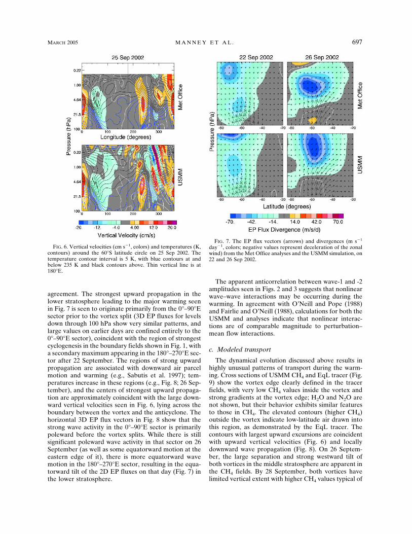
Temperature and vertical velocity (6-h averages cen-tered at 1200 UTC in the Met Office data and at 1200UTC in the USMM) cross sections (Fig. 6) show thatbaroclinic zones (regions of extremely strong tiltingtemperature gradients resembling upper-troposphericfronts) appear during the warming, forming as thewarming begins and strengthening until the vortexsplits, similar to those in simulations of NH majorwarmings (e.g., Fairlie et al. 1990a; Manney et al. 1994a,1999). The pattern of vertical velocities, with downwardmotion over and to the east and weak upward motionbelow and to the west of the baroclinic zone, acts tostrengthen the temperature gradients. Horizontal maps(not shown) indicate a dipole pattern of upward anddownward motion across the vortex edge as shown byManney et al. (1994a) for the NH. The narrow bands ofalternating upward and downward vertical velocitiesextending eastward and upward above the eastern

baroclinic zone strongly resemble features described byFairlie et al. (1990a) that they showed to be consistentwith inertio-gravity waves generated along the baro-clinic zone. The maximum vertical and horizontal tem-perature gradients [�10 K km�1 and �27 K (1000km)�1, respectively] are slightly larger than those re-ported by Fairlie et al. (1990a) and Manney et al.(1994a) for NH simulations.

Earlier studies (e.g., Manney et al. 1994a; Fairlie etal. 1990a) of NH warmings typically used NCEP CPCobjective analyses, other analyses based on TelevisionInfrared Observation Satellite (TIROS) OperationalVertical Sounder data, or simple analyses of Limb In-frared Monitor of the Stratosphere satellite tempera-ture data to compare with simulations, as opposed tothe analyses used here that are based on assimilationmodels using a comprehensive general circulationmodel (GCM). While the data ingested are similar, theuse of a GCM in the assimilation process can refinesmall-scale structure such as baroclinic zones thatwould not be well resolved in simpler analyses of coarseresolution data. The Met Office analyses show horizon-

FIG. 2. Time series of Met Office and USMM (top to bottom) 10-hPa zonal-mean winds, zonal-mean temperatures, and wave-1 and -2 geopotential heights. The wind contour interval is 5 m s�1,with values less than zero shaded. The temperature contour interval is 2.5 K, with 215–225 K darklyshaded and values over 240 K lightly shaded. The wave-1 contour interval is 200 m, with 800–1000 mshaded; the wave-2 contour interval is 100 m, with 400–500 m shaded. Dots in wave-1 and -2 plotsindicate the phase (longitude of one maximum) at 60°S.


tal and vertical temperature gradients comparable tothose generated in the USMM, in contrast to earliercomparisons where the analyses used did not fullyresolve baroclinic zones. Simmons et al. (2005) alsodemonstrate the ability of the ECMWF assimilationproducts to capture small-scale structure. The USMM,however, provides a more realistic representation ofthe temperature structure near the stratopause, wherethe Met Office assimilation system is at a disadvan-tage in being near the top of the analysis system andwhere the data ingested are increasingly sparse and un-certain.

b. Diagnostics of wave propagationand interactions

Eliassen–Palm fluxes serve as indicators of wavepropagation and wave–mean flow interactions. Figure 7shows cross sections of EP flux and divergence from theanalyses and the USMM leading up to and after thevortex split. Strong upward propagation and somezonal-wind deceleration throughout the high-latitudestratosphere begins on �20 September, and by 22 Sep-

tember, upward propagation intensifies, with fluxes di-rected poleward in the lower to middle stratosphere.Zonal-wind deceleration intensifies through 26 Septem-ber, with maximum deceleration moving to lower lati-tudes in a progressively broader region as upward-propagating waves are steered equatorward. After 26September, wave propagation is directed equatorwardin the lower stratosphere, and acceleration of the zonalmean winds begins in the upper stratosphere. Exami-nation of the indices of refraction for waves 1 and 2 (notshown) indicates a broad corridor for upward and pole-ward propagation throughout the stratosphere for bothwaves (narrower on the poleward side for wave 2) priorto the warming, with maximum deceleration beginningalong the poleward boundary in the upper stratosphere;the region narrows on the poleward side and cuts off inthe midstratosphere as the winds reverse. This is con-sistent with the poleward direction of the fluxes on 22September, and the equatorward tilt and broader, butlower-altitude, region of deceleration seen on 26 Sep-tember.The longitudinal distribution of propagation isshown in the 3D EP fluxes (Fig. 8). The patterns of 3DEP flux in the USMM and analyses are in very good

FIG. 3. Time series of Met Office and USMM 60°S (top to bottom) zonal-mean winds, zonal-meantemperatures, and wave-1 and -2 geopotential heights. The wind contour interval is 10 m s�1, withvalues less than zero shaded. The temperature contour interval is 3.0 K, with 216–225 K lightlyshaded and 234–240 K darkly shaded. The wave-1 contour interval is 150 m, with 600–750 m shaded;the wave-2 contour interval is 100 m, with 500–600 m shaded.


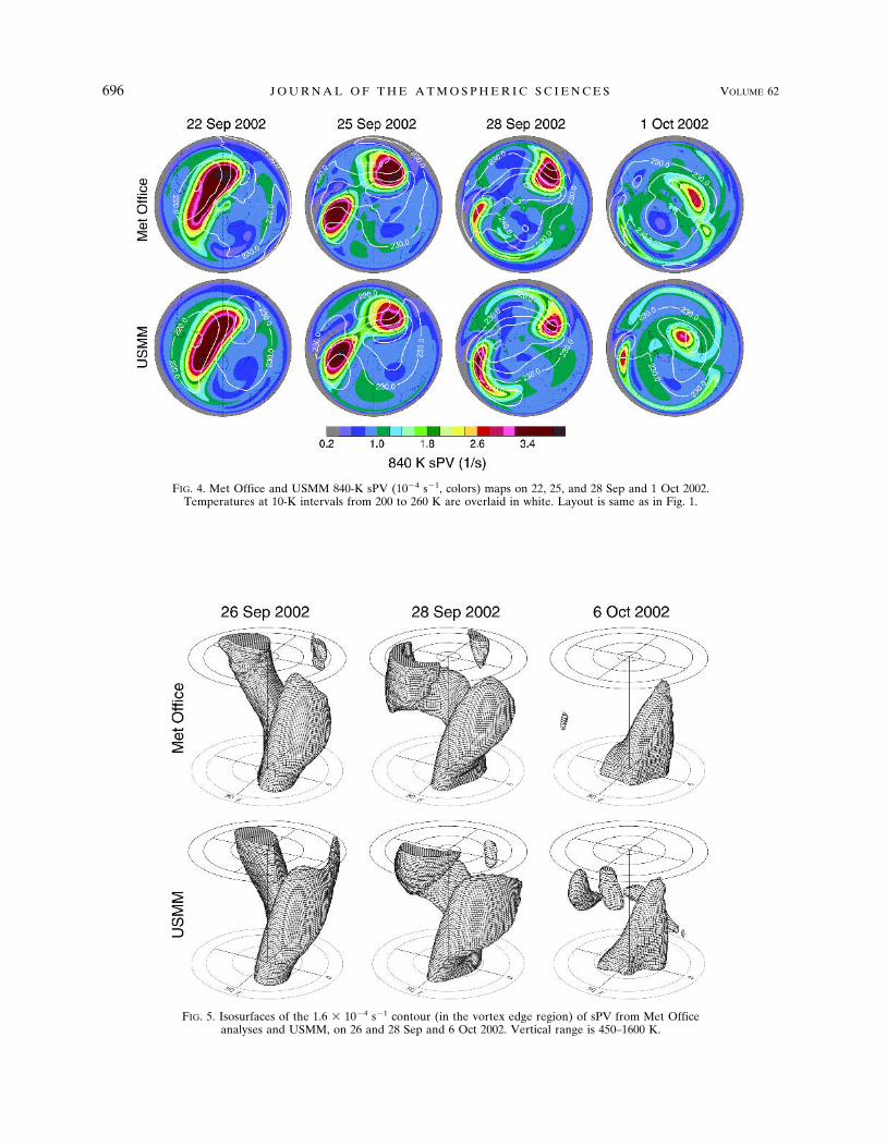
FIG. 4. Met Office and USMM 840-K sPV (10�4 s�1, colors) maps on 22, 25, and 28 Sep and 1 Oct 2002.Temperatures at 10-K intervals from 200 to 260 K are overlaid in white. Layout is same as in Fig. 1.

FIG. 5. Isosurfaces of the 1.6 � 10�4 s�1 contour (in the vortex edge region) of sPV from Met Officeanalyses and USMM, on 26 and 28 Sep and 6 Oct 2002. Vertical range is 450–1600 K.


Fig 4 live 4/C

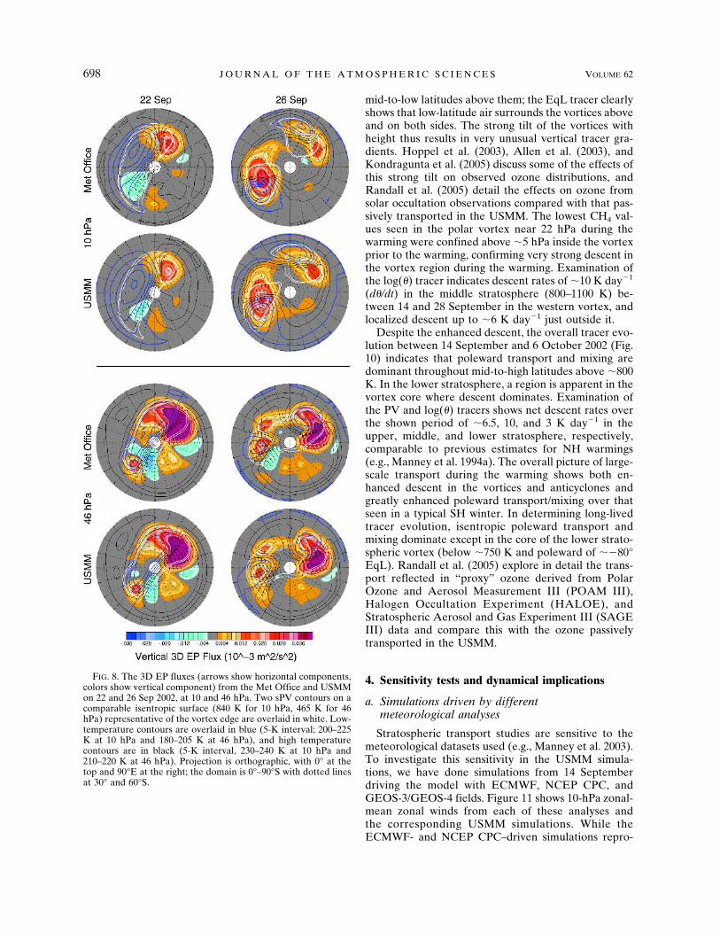
agreement. The strongest upward propagation in thelower stratosphere leading to the major warming seenin Fig. 7 is seen to originate primarily from the 0°–90°Esector prior to the vortex split (3D EP fluxes for levelsdown through 100 hPa show very similar patterns, andlarge values on earlier days are confined entirely to the0°–90°E sector), coincident with the region of strongestcyclogenesis in the boundary fields shown in Fig. 1, witha secondary maximum appearing in the 180°–270°E sec-tor after 22 September. The regions of strong upwardpropagation are associated with downward air parcelmotion and warming (e.g., Sabutis et al. 1997); tem-peratures increase in these regions (e.g., Fig. 8; 26 Sep-tember), and the centers of strongest upward propaga-tion are approximately coincident with the large down-ward vertical velocities seen in Fig. 6, lying across theboundary between the vortex and the anticyclone. Thehorizontal 3D EP flux vectors in Fig. 8 show that thestrong wave activity in the 0°–90°E sector is primarilypoleward before the vortex splits. While there is stillsignificant poleward wave activity in that sector on 26September (as well as some equatorward motion at theeastern edge of it), there is more equatorward wavemotion in the 180°–270°E sector, resulting in the equa-torward tilt of the 2D EP fluxes on that day (Fig. 7) inthe lower stratosphere.

The apparent anticorrelation between wave-1 and -2amplitudes seen in Figs. 2 and 3 suggests that nonlinearwave–wave interactions may be occurring during thewarming. In agreement with O’Neill and Pope (1988)and Fairlie and O’Neill (1988), calculations for both theUSMM and analyses indicate that nonlinear interac-tions are of comparable magnitude to perturbation–mean flow interactions.

c. Modeled transport

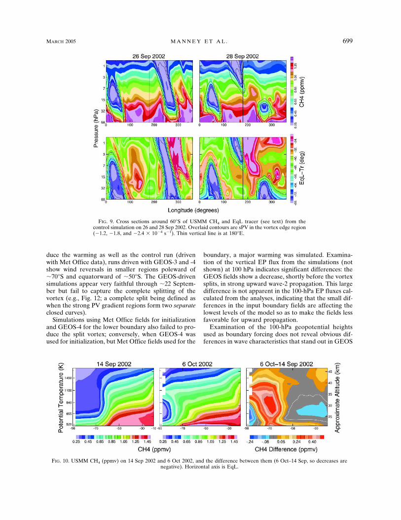
The dynamical evolution discussed above results inhighly unusual patterns of transport during the warm-ing. Cross sections of USMM CH4 and EqL tracer (Fig.9) show the vortex edge clearly defined in the tracerfields, with very low CH4 values inside the vortex andstrong gradients at the vortex edge; H2O and N2O arenot shown, but their behavior exhibits similar featuresto those in CH4. The elevated contours (higher CH4)outside the vortex indicate low-latitude air drawn intothis region, as demonstrated by the EqL tracer. Thecontours with largest upward excursions are coincidentwith upward vertical velocities (Fig. 6) and locallydownward wave propagation (Fig. 8). On 26 Septem-ber, the large separation and strong westward tilt ofboth vortices in the middle stratosphere are apparent inthe CH4 fields. By 28 September, both vortices havelimited vertical extent with higher CH4 values typical of

FIG. 6. Vertical velocities (cm s�1, colors) and temperatures (K,contours) around the 60°S latitude circle on 25 Sep 2002. Thetemperature contour interval is 5 K, with blue contours at andbelow 235 K and black contours above. Thin vertical line is at180°E.

FIG. 7. The EP flux vectors (arrows) and divergences (m s�1

day�1, colors; negative values represent deceleration of the zonalwind) from the Met Office analyses and the USMM simulation, on22 and 26 Sep 2002.


Fig 6 7 live 4/C

mid-to-low latitudes above them; the EqL tracer clearlyshows that low-latitude air surrounds the vortices aboveand on both sides. The strong tilt of the vortices withheight thus results in very unusual vertical tracer gra-dients. Hoppel et al. (2003), Allen et al. (2003), andKondragunta et al. (2005) discuss some of the effects ofthis strong tilt on observed ozone distributions, andRandall et al. (2005) detail the effects on ozone fromsolar occultation observations compared with that pas-sively transported in the USMM. The lowest CH4 val-ues seen in the polar vortex near 22 hPa during thewarming were confined above �5 hPa inside the vortexprior to the warming, confirming very strong descent inthe vortex region during the warming. Examination ofthe log(�) tracer indicates descent rates of �10 K day�1

(d�/dt) in the middle stratosphere (800–1100 K) be-tween 14 and 28 September in the western vortex, andlocalized descent up to �6 K day�1 just outside it.

Despite the enhanced descent, the overall tracer evo-lution between 14 September and 6 October 2002 (Fig.10) indicates that poleward transport and mixing aredominant throughout mid-to-high latitudes above �800K. In the lower stratosphere, a region is apparent in thevortex core where descent dominates. Examination ofthe PV and log(�) tracers shows net descent rates overthe shown period of �6.5, 10, and 3 K day�1 in theupper, middle, and lower stratosphere, respectively,comparable to previous estimates for NH warmings(e.g., Manney et al. 1994a). The overall picture of large-scale transport during the warming shows both en-hanced descent in the vortices and anticyclones andgreatly enhanced poleward transport/mixing over thatseen in a typical SH winter. In determining long-livedtracer evolution, isentropic poleward transport andmixing dominate except in the core of the lower strato-spheric vortex (below �750 K and poleward of ��80°EqL). Randall et al. (2005) explore in detail the trans-port reflected in “proxy” ozone derived from PolarOzone and Aerosol Measurement III (POAM III),Halogen Occultation Experiment (HALOE), andStratospheric Aerosol and Gas Experiment III (SAGEIII) data and compare this with the ozone passivelytransported in the USMM.

4. Sensitivity tests and dynamical implications

a. Simulations driven by differentmeteorological analyses

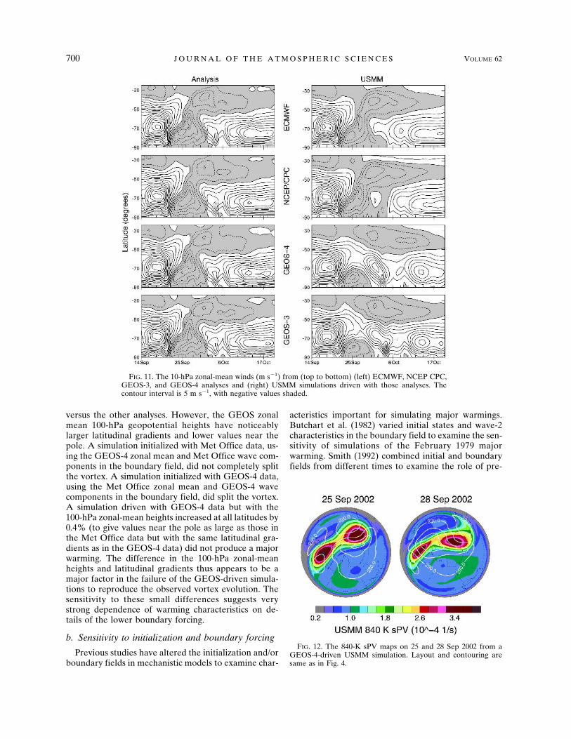
Stratospheric transport studies are sensitive to themeteorological datasets used (e.g., Manney et al. 2003).To investigate this sensitivity in the USMM simula-tions, we have done simulations from 14 Septemberdriving the model with ECMWF, NCEP CPC, andGEOS-3/GEOS-4 fields. Figure 11 shows 10-hPa zonal-mean zonal winds from each of these analyses andthe corresponding USMM simulations. While theECMWF- and NCEP CPC–driven simulations repro-

FIG. 8. The 3D EP fluxes (arrows show horizontal components,colors show vertical component) from the Met Office and USMMon 22 and 26 Sep 2002, at 10 and 46 hPa. Two sPV contours on acomparable isentropic surface (840 K for 10 hPa, 465 K for 46hPa) representative of the vortex edge are overlaid in white. Low-temperature contours are overlaid in blue (5-K interval; 200–225K at 10 hPa and 180–205 K at 46 hPa), and high temperaturecontours are in black (5-K interval, 230–240 K at 10 hPa and210–220 K at 46 hPa). Projection is orthographic, with 0° at thetop and 90°E at the right; the domain is 0°–90°S with dotted linesat 30° and 60°S.


Fig 8 live 4/C

duce the warming as well as the control run (drivenwith Met Office data), runs driven with GEOS-3 and -4show wind reversals in smaller regions poleward of�70°S and equatorward of �50°S. The GEOS-drivensimulations appear very faithful through �22 Septem-ber but fail to capture the complete splitting of thevortex (e.g., Fig. 12; a complete split being defined aswhen the strong PV gradient regions form two separateclosed curves).

Simulations using Met Office fields for initializationand GEOS-4 for the lower boundary also failed to pro-duce the split vortex; conversely, when GEOS-4 wasused for initialization, but Met Office fields used for the

boundary, a major warming was simulated. Examina-tion of the vertical EP flux from the simulations (notshown) at 100 hPa indicates significant differences: theGEOS fields show a decrease, shortly before the vortexsplits, in strong upward wave-2 propagation. This largedifference is not apparent in the 100-hPa EP fluxes cal-culated from the analyses, indicating that the small dif-ferences in the input boundary fields are affecting thelowest levels of the model so as to make the fields lessfavorable for upward propagation.

Examination of the 100-hPa geopotential heightsused as boundary forcing does not reveal obvious dif-ferences in wave characteristics that stand out in GEOS

FIG. 10. USMM CH4 (ppmv) on 14 Sep 2002 and 6 Oct 2002, and the difference between them (6 Oct–14 Sep, so decreases arenegative). Horizontal axis is EqL.

FIG. 9. Cross sections around 60°S of USMM CH4 and EqL tracer (see text) from thecontrol simulation on 26 and 28 Sep 2002. Overlaid contours are sPV in the vortex edge region(�1.2, �1.8, and �2.4 � 10�4 s�1). Thin vertical line is at 180°E.


Fig 9 10 live 4/C

versus the other analyses. However, the GEOS zonalmean 100-hPa geopotential heights have noticeablylarger latitudinal gradients and lower values near thepole. A simulation initialized with Met Office data, us-ing the GEOS-4 zonal mean and Met Office wave com-ponents in the boundary field, did not completely splitthe vortex. A simulation initialized with GEOS-4 data,using the Met Office zonal mean and GEOS-4 wavecomponents in the boundary field, did split the vortex.A simulation driven with GEOS-4 data but with the100-hPa zonal-mean heights increased at all latitudes by0.4% (to give values near the pole as large as those inthe Met Office data but with the same latitudinal gra-dients as in the GEOS-4 data) did not produce a majorwarming. The difference in the 100-hPa zonal-meanheights and latitudinal gradients thus appears to be amajor factor in the failure of the GEOS-driven simula-tions to reproduce the observed vortex evolution. Thesensitivity to these small differences suggests verystrong dependence of warming characteristics on de-tails of the lower boundary forcing.

b. Sensitivity to initialization and boundary forcing

Previous studies have altered the initialization and/orboundary fields in mechanistic models to examine char-

acteristics important for simulating major warmings.Butchart et al. (1982) varied initial states and wave-2characteristics in the boundary field to examine the sen-sitivity of simulations of the February 1979 majorwarming. Smith (1992) combined initial and boundaryfields from different times to examine the role of pre-

FIG. 12. The 840-K sPV maps on 25 and 28 Sep 2002 from aGEOS-4-driven USMM simulation. Layout and contouring aresame as in Fig. 4.

FIG. 11. The 10-hPa zonal-mean winds (m s�1) from (top to bottom) (left) ECMWF, NCEP CPC,GEOS-3, and GEOS-4 analyses and (right) USMM simulations driven with those analyses. Thecontour interval is 5 m s�1, with negative values shaded.


Fig 12 live 4/C

conditioning in the occurrence of major warmings.Here, sensitivity tests varying the Met Office fields usedfor initialization and boundary forcing (described be-low and summarized in Table 1) help us to understandwhat characteristics of the driving fields are importantin simulating the SH major warming. The results showstrong sensitivity to boundary forcing and to some char-acteristics of the initialization fields.

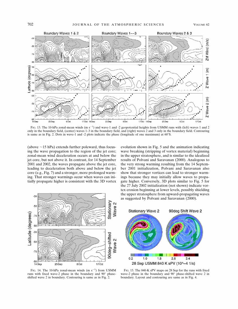
When only waves 1 and 2 are included in the bound-ary field, the vortex does not completely split and thereis no wind reversal near 60°S (Fig. 13); with waves 1–3or waves 2–3 in the boundary field, the warmingstrongly resembles that observed (Fig. 13). When the100-hPa wave 1 is excluded, the wave-2 amplitude at 10hPa grows nearly monotonically until �25 Septemberand decays smoothly thereafter, and winds recovermore slowly and weakly near the pole (Fig. 13). Thissupports the idea that the vacillation in wave-2 ampli-tudes seen in the control run may arise from nonlinearinteractions between wave 1 and wave 2; it also indi-cates that the vacillation is not needed for the majorwarming to occur but does play a significant role in therecovery, similar to the results of Jung et al. (2001) forthe NH February 1979 warming. In runs with alteredwave-2 phases (Fig. 14), a major warming occurs but ismore dominated by wave 1 (Fig. 15), and the vortexdoes not split until 30 September–2 October. No runswith decreased boundary wave amplitudes resulted instrong warmings.

Figure 16 shows the 14 September zonal-mean windsfor the control run, runs initialized with 14 September1997 and 14 September 2001 fields, and the run initial-ized on 27 July 2002. These cases represent substantialdifferences in the strength and structure of the jet,

which affect wave propagation. On 14 September 2002,the jet is weak, and the vortex is relatively small (i.e.,the jet core is at high latitude); in 1997, the vortex iseven smaller, but the jet is stronger; in 2001, the vortexis both large and strong. The runs with earlier initial-izations (the 27 July initialization, in Fig. 16, is the ex-treme case) evolve so that, by 14 September, the vortexis smaller but stronger than that observed.

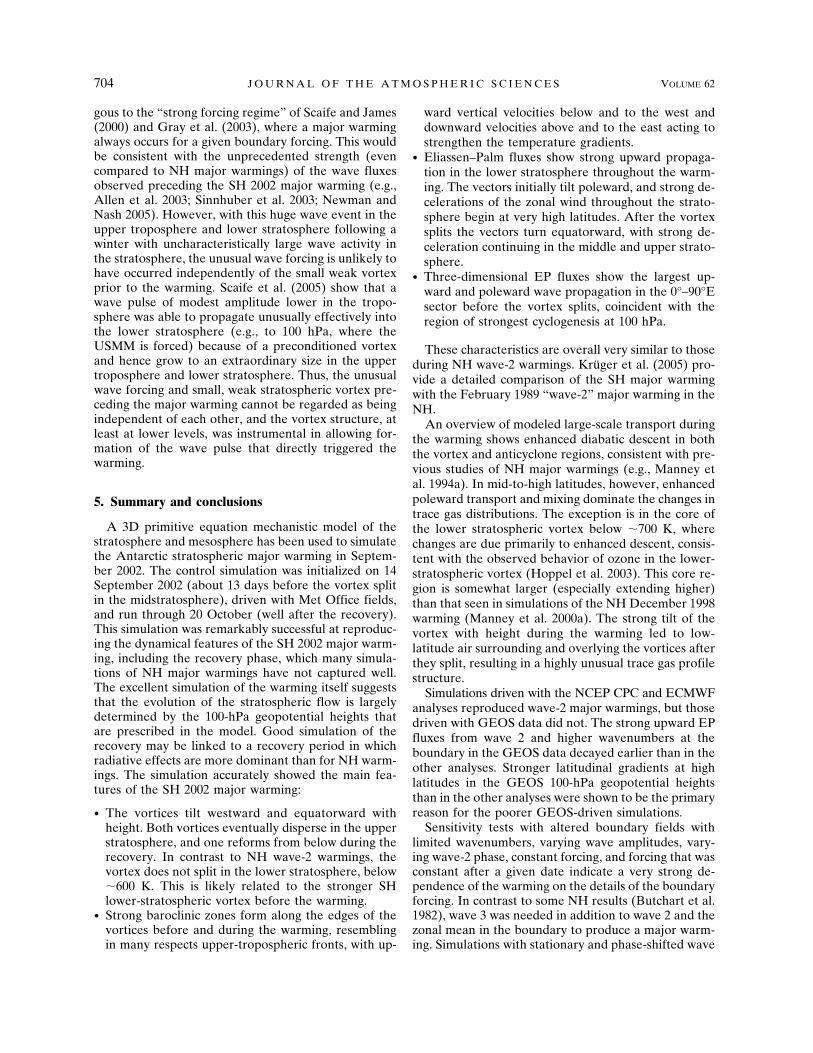
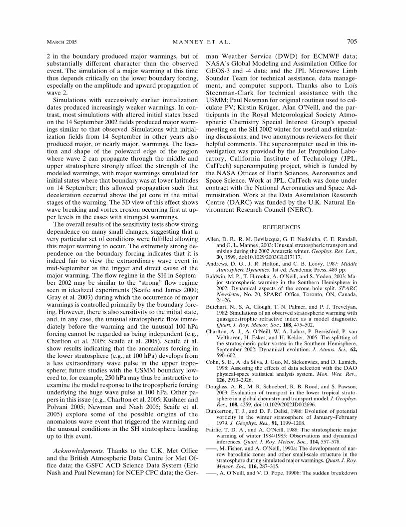
The run with the 2001 (large, strong vortex) initial-ization produces a wave-2 major warming that becomesstronger than that in the control run (Figs. 17 and 18) .The run with the 1997 initialization produces a verystrong, but not major, warming (Fig. 17), where thevortex nearly splits on 26 September (Fig. 18) but thenbegins to recover. Runs with a zonally symmetric initialstate based on 14 September 2002 (Fig. 17) and with thezonal-mean wind component enhanced in a 14 Septem-ber 2002–based initial state also produce major warm-ings. The vortex split in the run initialized on 11 Sep-tember 2002, but the two vortices were not as widelyseparated as in the control run, resulting in winds re-maining westerly in a small region poleward of 60°S;runs with progressively earlier initializations (29 and 11August, and 27 July) produced simulations without avortex split, with increasingly weaker (though still verystrong by SH standards) wave-1-dominated warmings.Thus, the cumulative effect of small discrepancies de-veloping in the model alters the jet structure to be lessfavorable to the wave propagation resulting in thewarming.

Examination of wave activity and refractive indices(Fig. 16 also shows the wave-2 refractive index) indi-cates that, for smaller vortices, the region where wave 2propagates through the middle and upper stratosphere

TABLE 1. USMM sensitivity tests to different boundary and initial conditions.

Initial date Initial field Boundary field Results

Sensitivity to boundary forcing

14 Sep 2002 Met Office data Zonal mean � waves 1–2 Strong warming14 Sep 2002 Met Office data Zonal mean � waves 1–3 Major warming14 Sep 2002 Met Office data Zonal mean � waves 2–3 Major warming14 Sep 2002 Met Office data Wave 2 stationary Major wave-1, -2 warming14 Sep 2002 Met Office data Wave 2 shifted 90° Major wave-1, -2 warming14 Sep 2002 Met Office data 0.5 � wave 1–6 A No significant warming14 Sep 2002 Met Office data 0.75 � wave 1–6 A Minor warming14 Sep 2002 Met Office data Const field, avg 30 days before initial No warming14 Sep 2002 Met Office data Const field, 22 Sep zonal mean � 0.6

� wave 1–6 AMinor warming

14 Sep 2002 Met Office data Met Office data through 22 Sep, constantthereafter at 22 Sep value

Later major wave-1 warming

Sensitivity to initial conditions

11 Sep 2002 Met Office data Met Office data Strong wave-2 warming17 Sep 2002 Met Office data Met Office data Weaker major wave-2 warmingEarlier Inits Met Office data Met Office data Strong wave-2 warming14 Sep 2002 1.1 � zonal-mean winds Met Office data Major wave-2 warming14 Sep 2002 1.25 � zonal-mean winds Met Office data Major wave-2 warming14 Sep 2002 Zonal mean only Met Office data Major wave-2 warming14 Sep 1997 Met Office data Sep–Oct 2002 Met Office data Strong wave-2 warming14 Sep 2001 Met Office data Sep–Oct 2002 Met Office data Major wave-2 warming


(above �15 hPa) extends further poleward, thus focus-ing the wave propagation to the region of the jet core;zonal-mean wind deceleration occurs at and below thejet core, but not above it. In contrast, for 14 September2001 and 2002, the waves propagate above the jet core,leading to deceleration both above and below the jetcore (e.g., Fig. 7) and a stronger, more prolonged warm-ing. That stronger warmings occur when waves can ini-tially propagate higher is consistent with the 3D vortex

evolution shown in Fig. 5 and the animation indicatingwave breaking (stripping of vortex material) beginningin the upper stratosphere, and is similar to the idealizedresults of Polvani and Saravanan (2000). Analogous tothe very strong warming resulting from the 14 Septem-ber 2001 initialization, Polvani and Saravanan alsoshow that stronger vortices can lead to stronger warm-ings because they may initially allow waves to propa-gate higher. Conversely, 3D plots similar to Fig. 5 forthe 27 July 2002 initialization (not shown) indicate vor-tex erosion beginning at lower levels, possibly shieldingthe upper stratosphere from upward-propagating wavesas suggested by Polvani and Saravanan (2000).

FIG. 13. The 10-hPa zonal-mean winds (m s�1) and wave-1 and -2 geopotential heights from USMM runs with (left) waves 1 and 2only in the boundary field, (center) waves 1–3 in the boundary field, and (right) waves 2 and 3 only in the boundary field. Contouringis same as in Fig. 2. Dots in wave-1 and -2 plots indicate the phase (longitude of one maximum) at 60°S.

FIG. 14. The 10-hPa zonal-mean winds (m s�1) from USMMruns with fixed wave-2 phase in the boundary and 90° phase-shifted wave 2 in boundary. Contouring is same as in Fig. 2.

FIG. 15. The 840-K sPV maps on 28 Sep for the runs with fixedwave-2 phase in the boundary and 90° phase-shifted wave 2 inboundary. Layout and contouring are same as in Fig. 4.


Fig 15 live 4/C

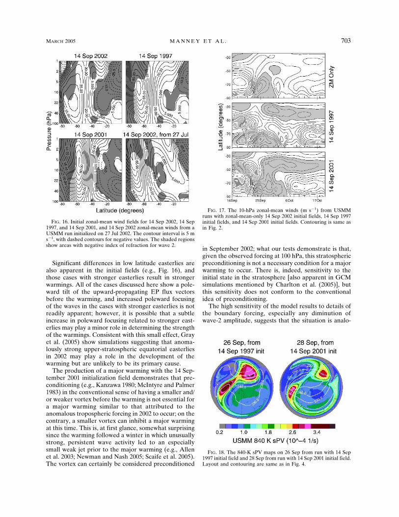
Significant differences in low latitude easterlies arealso apparent in the initial fields (e.g., Fig. 16), andthose cases with stronger easterlies result in strongerwarmings. All of the cases discussed here show a pole-ward tilt of the upward-propagating EP flux vectorsbefore the warming, and increased poleward focusingof the waves in the cases with stronger easterlies is notreadily apparent; however, it is possible that a subtleincrease in poleward focusing related to stronger east-erlies may play a minor role in determining the strengthof the warmings. Consistent with this small effect, Grayet al. (2005) show simulations suggesting that anoma-lously strong upper-stratospheric equatorial easterliesin 2002 may play a role in the development of thewarming but are unlikely to be its primary cause.

The production of a major warming with the 14 Sep-tember 2001 initialization field demonstrates that pre-conditioning (e.g., Kanzawa 1980; McIntyre and Palmer1983) in the conventional sense of having a smaller and/or weaker vortex before the warming is not essential fora major warming similar to that attributed to theanomalous tropospheric forcing in 2002 to occur; on thecontrary, a smaller vortex can inhibit a major warmingat this time. This is, at first glance, somewhat surprisingsince the warming followed a winter in which unusuallystrong, persistent wave activity led to an especiallysmall weak jet prior to the major warming (e.g., Allenet al. 2003; Newman and Nash 2005; Scaife et al. 2005).The vortex can certainly be considered preconditioned

in September 2002; what our tests demonstrate is that,given the observed forcing at 100 hPa, this stratosphericpreconditioning is not a necessary condition for a majorwarming to occur. There is, indeed, sensitivity to theinitial state in the stratosphere [also apparent in GCMsimulations mentioned by Charlton et al. (2005)], butthis sensitivity does not conform to the conventionalidea of preconditioning.

The high sensitivity of the model results to details ofthe boundary forcing, especially any diminution ofwave-2 amplitude, suggests that the situation is analo-

FIG. 16. Initial zonal-mean wind fields for 14 Sep 2002, 14 Sep1997, and 14 Sep 2001, and 14 Sep 2002 zonal-mean winds from aUSMM run initialized on 27 Jul 2002. The contour interval is 5 ms�1, with dashed contours for negative values. The shaded regionsshow areas with negative index of refraction for wave 2.

FIG. 17. The 10-hPa zonal-mean winds (m s�1) from USMMruns with zonal-mean-only 14 Sep 2002 initial fields, 14 Sep 1997initial fields, and 14 Sep 2001 initial fields. Contouring is same asin Fig. 2.

FIG. 18. The 840-K sPV maps on 26 Sep from run with 14 Sep1997 initial field and 28 Sep from run with 14 Sep 2001 initial field.Layout and contouring are same as in Fig. 4.


Fig 18 live 4/C

gous to the “strong forcing regime” of Scaife and James(2000) and Gray et al. (2003), where a major warmingalways occurs for a given boundary forcing. This wouldbe consistent with the unprecedented strength (evencompared to NH major warmings) of the wave fluxesobserved preceding the SH 2002 major warming (e.g.,Allen et al. 2003; Sinnhuber et al. 2003; Newman andNash 2005). However, with this huge wave event in theupper troposphere and lower stratosphere following awinter with uncharacteristically large wave activity inthe stratosphere, the unusual wave forcing is unlikely tohave occurred independently of the small weak vortexprior to the warming. Scaife et al. (2005) show that awave pulse of modest amplitude lower in the tropo-sphere was able to propagate unusually effectively intothe lower stratosphere (e.g., to 100 hPa, where theUSMM is forced) because of a preconditioned vortexand hence grow to an extraordinary size in the uppertroposphere and lower stratosphere. Thus, the unusualwave forcing and small, weak stratospheric vortex pre-ceding the major warming cannot be regarded as beingindependent of each other, and the vortex structure, atleast at lower levels, was instrumental in allowing for-mation of the wave pulse that directly triggered thewarming.

5. Summary and conclusions

A 3D primitive equation mechanistic model of thestratosphere and mesosphere has been used to simulatethe Antarctic stratospheric major warming in Septem-ber 2002. The control simulation was initialized on 14September 2002 (about 13 days before the vortex splitin the midstratosphere), driven with Met Office fields,and run through 20 October (well after the recovery).This simulation was remarkably successful at reproduc-ing the dynamical features of the SH 2002 major warm-ing, including the recovery phase, which many simula-tions of NH major warmings have not captured well.The excellent simulation of the warming itself suggeststhat the evolution of the stratospheric flow is largelydetermined by the 100-hPa geopotential heights thatare prescribed in the model. Good simulation of therecovery may be linked to a recovery period in whichradiative effects are more dominant than for NH warm-ings. The simulation accurately showed the main fea-tures of the SH 2002 major warming:

• The vortices tilt westward and equatorward withheight. Both vortices eventually disperse in the upperstratosphere, and one reforms from below during therecovery. In contrast to NH wave-2 warmings, thevortex does not split in the lower stratosphere, below�600 K. This is likely related to the stronger SHlower-stratospheric vortex before the warming.

• Strong baroclinic zones form along the edges of thevortices before and during the warming, resemblingin many respects upper-tropospheric fronts, with up-

ward vertical velocities below and to the west anddownward velocities above and to the east acting tostrengthen the temperature gradients.

• Eliassen–Palm fluxes show strong upward propaga-tion in the lower stratosphere throughout the warm-ing. The vectors initially tilt poleward, and strong de-celerations of the zonal wind throughout the strato-sphere begin at very high latitudes. After the vortexsplits the vectors turn equatorward, with strong de-celeration continuing in the middle and upper strato-sphere.

• Three-dimensional EP fluxes show the largest up-ward and poleward wave propagation in the 0°–90°Esector before the vortex splits, coincident with theregion of strongest cyclogenesis at 100 hPa.

These characteristics are overall very similar to thoseduring NH wave-2 warmings. Krüger et al. (2005) pro-vide a detailed comparison of the SH major warmingwith the February 1989 “wave-2” major warming in theNH.

An overview of modeled large-scale transport duringthe warming shows enhanced diabatic descent in boththe vortex and anticyclone regions, consistent with pre-vious studies of NH major warmings (e.g., Manney etal. 1994a). In mid-to-high latitudes, however, enhancedpoleward transport and mixing dominate the changes intrace gas distributions. The exception is in the core ofthe lower stratospheric vortex below �700 K, wherechanges are due primarily to enhanced descent, consis-tent with the observed behavior of ozone in the lower-stratospheric vortex (Hoppel et al. 2003). This core re-gion is somewhat larger (especially extending higher)than that seen in simulations of the NH December 1998warming (Manney et al. 2000a). The strong tilt of thevortex with height during the warming led to low-latitude air surrounding and overlying the vortices afterthey split, resulting in a highly unusual trace gas profilestructure.

Simulations driven with the NCEP CPC and ECMWFanalyses reproduced wave-2 major warmings, but thosedriven with GEOS data did not. The strong upward EPfluxes from wave 2 and higher wavenumbers at theboundary in the GEOS data decayed earlier than in theother analyses. Stronger latitudinal gradients at highlatitudes in the GEOS 100-hPa geopotential heightsthan in the other analyses were shown to be the primaryreason for the poorer GEOS-driven simulations.

Sensitivity tests with altered boundary fields withlimited wavenumbers, varying wave amplitudes, vary-ing wave-2 phase, constant forcing, and forcing that wasconstant after a given date indicate a very strong de-pendence of the warming on the details of the boundaryforcing. In contrast to some NH results (Butchart et al.1982), wave 3 was needed in addition to wave 2 and thezonal mean in the boundary to produce a major warm-ing. Simulations with stationary and phase-shifted wave


2 in the boundary produced major warmings, but ofsubstantially different character than the observedevent. The simulation of a major warming at this timethus depends critically on the lower boundary forcing,especially on the amplitude and upward propagation ofwave 2.

Simulations with successively earlier initializationdates produced increasingly weaker warmings. In con-trast, most simulations with altered initial states basedon the 14 September 2002 fields produced major warm-ings similar to that observed. Simulations with initial-ization fields from 14 September in other years alsoproduced major, or nearly major, warmings. The loca-tion and shape of the poleward edge of the regionwhere wave 2 can propagate through the middle andupper stratosphere strongly affect the strength of themodeled warmings, with major warmings simulated forinitial states where that boundary was at lower latitudeson 14 September; this allowed propagation such thatdeceleration occurred above the jet core in the initialstages of the warming. The 3D view of this effect showswave breaking and vortex erosion occurring first at up-per levels in the cases with strongest warmings.

The overall results of the sensitivity tests show strongdependence on many small changes, suggesting that avery particular set of conditions were fulfilled allowingthis major warming to occur. The extremely strong de-pendence on the boundary forcing indicates that it isindeed fair to view the extraordinary wave event inmid-September as the trigger and direct cause of themajor warming. The flow regime in the SH in Septem-ber 2002 may be similar to the “strong” flow regimeseen in idealized experiments (Scaife and James 2000;Gray et al. 2003) during which the occurrence of majorwarmings is controlled primarily by the boundary forc-ing. However, there is also sensitivity to the initial state,and, in any case, the unusual stratospheric flow imme-diately before the warming and the unusual 100-hPaforcing cannot be regarded as being independent (e.g.,Charlton et al. 2005; Scaife et al. 2005). Scaife et al.show results indicating that the anomalous forcing inthe lower stratosphere (e.g., at 100 hPa) develops froma less extraordinary wave pulse in the upper tropo-sphere; future studies with the USMM boundary low-ered to, for example, 250 hPa may thus be instructive toexamine the model response to the tropospheric forcingunderlying the huge wave pulse at 100 hPa. Other pa-pers in this issue (e.g., Charlton et al. 2005; Kushner andPolvani 2005; Newman and Nash 2005; Scaife et al.2005) explore some of the possible origins of theanomalous wave event that triggered the warming andthe unusual conditions in the SH stratosphere leadingup to this event.

Acknowledgments. Thanks to the U.K. Met Officeand the British Atmospheric Data Centre for Met Of-fice data; the GSFC ACD Science Data System (EricNash and Paul Newman) for NCEP CPC data; the Ger-

man Weather Service (DWD) for ECMWF data;NASA’s Global Modeling and Assimilation Office forGEOS-3 and -4 data; and the JPL Microwave LimbSounder Team for technical assistance, data manage-ment, and computer support. Thanks also to LoïsSteenman-Clark for technical assistance with theUSMM; Paul Newman for original routines used to cal-culate PV; Kirstin Krüger, Alan O’Neill, and the par-ticipants in the Royal Meteorological Society Atmo-spheric Chemistry Special Interest Group’s specialmeeting on the SH 2002 winter for useful and stimulat-ing discussions; and two anonymous reviewers for theirhelpful comments. The supercomputer used in this in-vestigation was provided by the Jet Propulsion Labo-ratory, California Institute of Technology (JPL,CalTech) supercomputing project, which is funded bythe NASA Offices of Earth Sciences, Aeronautics andSpace Science. Work at JPL, CalTech was done undercontract with the National Aeronautics and Space Ad-ministration. Work at the Data Assimilation ResearchCentre (DARC) was funded by the U.K. Natural En-vironment Research Council (NERC).

REFERENCES

Allen, D. R., R. M. Bevilacqua, G. E. Nedoluha, C. E. Randall,and G. L. Manney, 2003: Unusual stratospheric transport andmixing during the 2002 Antarctic winter. Geophys. Res. Lett.,30, 1599, doi:10.1029/2003GL017117.

Andrews, D. G., J. R. Holton, and C. B. Leovy, 1987: MiddleAtmosphere Dynamics. 1st ed. Academic Press, 489 pp.

Baldwin, M. P., T. Hirooka, A. O’Neill, and S. Yoden, 2003: Ma-jor stratospheric warming in the Southern Hemisphere in2002: Dynamical aspects of the ozone hole split. SPARCNewsletter, No. 20, SPARC Office, Toronto, ON, Canada,24–26.

Butchart, N., S. A. Clough, T. N. Palmer, and P. J. Trevelyan,1982: Simulations of an observed stratospheric warming withquasigeostrophic refractive index as a model diagnostic.Quart. J. Roy. Meteor. Soc., 108, 475–502.

Charlton, A. J., A. O’Neill, W. A. Lahoz, P. Berrisford, P. vanVelthoven, H. Eskes, and H. Kelder, 2005: The splitting ofthe stratospheric polar vortex in the Southern Hemisphere,September 2002: Dynamical evolution. J. Atmos. Sci., 62,590–602.

Cohn, S. E., A. da Silva, J. Guo, M. Siekenwicz, and D. Lamich,1998: Assessing the effects of data selection with the DAOphysical-space statistical analysis system. Mon. Wea. Rev.,126, 2913–2926.

Douglass, A. R., M. R. Schoeberl, R. B. Rood, and S. Pawson,2003: Evaluation of transport in the lower tropical strato-sphere in a global chemistry and transport model. J. Geophys.Res., 108, 4259, doi:10.1029/2002JD002696.

Dunkerton, T. J., and D. P. Delisi, 1986: Evolution of potentialvorticity in the winter stratosphere of January–February1979. J. Geophys. Res., 91, 1199–1208.

Fairlie, T. D. A., and A. O’Neill, 1988: The stratospheric majorwarming of winter 1984/1985: Observations and dynamicalinferences. Quart. J. Roy. Meteor. Soc., 114, 557–578.

——, M. Fisher, and A. O’Neill, 1990a: The development of nar-row baroclinic zones and other small-scale structure in thestratosphere during simulated major warmings. Quart. J. Roy.Meteor. Soc., 116, 287–315.

——, A. O’Neill, and V. D. Pope, 1990b: The sudden breakdown


of an unusually strong cyclone in the stratosphere duringwinter 1988/89. Quart. J. Roy. Meteor. Soc., 116, 767–774.

Gray, L. J., S. Sparrow, M. Juckes, A. O’Neill, and D. G. An-drews, 2003: Flow regimes in the winter stratosphere of theNorthern Hemisphere. Quart. J. Roy. Meteor. Soc., 129, 925–945.

——, W. Norton, C. Pascoe, and A. Charlton, 2005: A possibleinfluence of equatorial winds on the September 2002 South-ern Hemisphere sudden warming event. J. Atmos. Sci., 62,651–667.

Hoppel, K. W., R. Bevilacqua, D. Allen, G. Nedoluha, and C.Randall, 2003: POAM III observations of the anomalous2002 Antarctic ozone hole. Geophys. Res. Lett., 30, 1394,doi:10.1029/2003GL016899.

Jung, J.-H., C. S. Konor, C. R. Mechoso, and A. Arakawa, 2001:A study of the stratospheric major warming and subsequentflow recovery during the winter of 1979 with an isentropicvertical coordinate model. J. Atmos. Sci., 58, 2630–2649.

Kanzawa, H., 1980: The behavior of mean zonal wind and plan-etary-scale disturbances in the troposphere and stratosphereduring the 1973 sudden warming. J. Meteor. Soc. Japan, 58,329–356.

Kondragunta, S., and Coauthors, 2005: Vertical structure of theanomalous 2002 Antarctic ozone hole. J. Atmos. Sci., 62, 801–811.

Krüger, K., B. Naujokat, and K. Labitzke, 2005: The unusual mid-winter warming in the Southern Hemisphere stratosphere of2002: A comparison to Northern Hemisphere phenomena. J.Atmos. Sci., 62, 603–613.

Kushner, P. J., and L. M. Polvani, 2005: A very large, spontaneousstratospheric sudden warming in a simple AGCM: A proto-type for the Southern Hemisphere warming of 2002? J. At-mos. Sci., 62, 890–897.

Labitzke, K., 1977: Interannual variability of the winter strato-sphere in the Northern Hemisphere. Mon. Wea. Rev., 105,762–770.

——, 1982: On the interannual variability of the middle strato-sphere during the northern winters. J. Meteor. Soc. Japan, 60,124–139.

Lin, S.-J., 2004: A “vertically Lagrangian” finite-volume dynami-cal core for global models. Mon. Wea. Rev., 132, 2293–2307.

MacKenzie, I. A., R. S. Harwood, P. A. Stott, and G. C. Watson,1999: Radiative-dynamic effects of the Antarctic ozone holeand chemical feedback. Quart. J. Roy. Meteor. Soc., 125,2171–2203.

Manney, G. L., J. D. Farrara, and C. R. Mechoso, 1994a: Simu-lations of the February 1979 stratospheric sudden warming:Model comparisons and three-dimensional evolution. Mon.Wea. Rev., 122, 1115–1140.

——, R. W. Zurek, A. O’Neill, and R. Swinbank, 1994b: On themotion of air through the stratospheric polar vortex. J. At-mos. Sci., 51, 2973–2994.

——, R. Swinbank, S. T. Massie, M. E. Gelman, A. J. Miller, R.Nagatani, A. O’Neill, and R. W. Zurek, 1996: Comparison ofU.K. Meteorological Office and U.S. National Meteorologi-cal Center stratospheric analyses during northern and south-ern winter. J. Geophys. Res., 101, 10 311–10 334.

——, W. A. Lahoz, R. Swinbank, A. O’Neill, P. M. Connew, andR. W. Zurek, 1999: Simulation of the December 1998 strato-spheric major warming. Geophys. Res. Lett., 26, 2733–2736.

——, R. M. Bevilacqua, K. W. Hoppel, W. A. Lahoz, A. O’Neill,and J. M. Russell III, 2000a: Observations and modeling oftransport during the December 1998 stratospheric majorwarming. Preprints, 11th Conf. on the Middle Atmosphere,Long Beach, CA, Amer. Meteor. Soc., 47.

——, H. A. Michelsen, F. W. Irion, M. R. Gunson, G. C. Toon,and A. E. Roche, 2000b: Lamination and polar vortex devel-opment in fall from ATMOS long-lived trace gases observedduring November 1994. J. Geophys. Res., 105, 29 023–29 038.

——, W. A. Lahoz, J. L. Sabutis, A. O’Neill, and L. Steenman-

Clark, 2002: Simulations of fall and early winter in the strato-sphere. Quart. J. Roy. Meteor. Soc., 128, 2205–2237.

——, J. L. Sabutis, S. Pawson, M. L. Santee, B. Naujokat, R.Swinbank, M. E. Gelman, and W. Ebisuzaki, 2003: Lowerstratospheric temperature differences between meteorologi-cal analyses in two cold Arctic winters and their impact onpolar processing studies. J. Geophys. Res., 108, 8328,doi:10.1029/2001JD001149.

Matsuno, T., 1970: Vertical propagation of stationary waves in thewinter Northern Hemisphere. J. Atmos. Sci., 27, 871–883.

McIntyre, M. E., and T. N. Palmer, 1983: Breaking planetarywaves in the stratosphere. Nature, 305, 593–600.

Naujokat, B., K. Krüger, K. Matthes, J. Hoffmann, M. Kunze, andK. Labitzke, 2002: The early major warming in December2001—Exceptional? Geophys. Res. Lett., 29, 2023,doi:10.1029/2002GL015316.

Newman, P. A., and E. R. Nash, 2005: The unusual SouthernHemisphere stratosphere winter of 2002. J. Atmos. Sci., 62,614–628.

——, L. R. Lait, M. R. Schoeberl, R. M. Nagatani, and A. J.Krueger, 1989: Meteorological atlas of the Northern Hemi-sphere lower stratosphere for January and February 1989during the Airborne Arctic Stratospheric Expedition. Tech.Rep. 4145, NASA.

O’Neill, A., and V. D. Pope, 1988: Simulations of linear and non-linear disturbances in the stratosphere. Quart. J. Roy. Meteor.Soc., 114, 1063–1110.

Plumb, R. A., 1985: On the three-dimensional propagation ofstationary waves. J. Atmos. Sci., 42, 217–229.

Polvani, L. M., and R. Saravanan, 2000: The three-dimensionalstructure of breaking Rossby waves in the polar wintertimestratosphere. J. Atmos. Sci., 57, 3663–3685.

Randall, C. E., G. L. Manney, D. R. Allen, R. M. Bevilacqua, C.Trepte, W. A. Lahoz, and A. O’Neill, 2005: Reconstructionand simulation of stratospheric ozone distributions during the2002 austral winter. J. Atmos. Sci., 62, 748–764.

Sabutis, J. L., 1997: The short-term transport of zonal mean ozoneusing a residual mean circulation calculated from observa-tions. J. Atmos. Sci., 54, 1094–1106.

——, R. P. Turco, and S. K. Kar, 1997: Wintertime planetary wavepropagation in the lower stratosphere and its observed effecton Northern Hemisphere temperature–ozone correlations. J.Geophys. Res., 102, 21 709–21 717.

Scaife, A. A., and I. N. James, 2000: Response of the stratosphereto interannual variability of tropospheric planetary waves.Quart. J. Roy. Meteor. Soc., 126, 275–297.

——, R. Swinbank, D. R. Jackson, N. Butchart, H. Thornton, M.Keil, and L. Henderson, 2005: Stratospheric vacillations andthe major warming over Antarctica in 2002. J. Atmos. Sci., 62,629–639.

Schoeberl, M. R., A. R. Douglass, Z. Zhu, and S. Pawson, 2003: Acomparison of the lower stratospheric age spectra derivedfrom a general circulation model and two data assimilationsystems. J. Geophys. Res., 108, 4113, doi:10.1029/2002JD002652.

Scott, R. K., and P. H. Haynes, 1998: Internal interannual vari-ability of the extratropical stratospheric circulation: The low-latitude flywheel. Quart. J. Roy. Meteor. Soc., 124, 2149–2173.

Shine, K. P., 1987: The middle atmosphere in the absence of dy-namic heat fluxes. Quart. J. Roy. Meteor. Soc., 113, 603–633.

Simmons, A. J., M. Hortal, G. Kelly, A. McNally, A. Untch, andS. Uppala, 2005: ECMWF analyses and forecasts of strato-spheric winter polar vortex breakup: September 2002 in theSouthern Hemisphere and related events. J. Atmos. Sci., 62,668–689.

Sinnhuber, B.-M., M. Weber, A. Amankwah, and J. P. Burrows,2003: Total ozone during the unusual Antarctic winter of2002. Geophys. Res. Lett . , 30, 1580, doi:10.1029/2002GL016798.


Smith, A. K., 1992: Preconditioning for stratospheric suddenwarmings: Sensitivity studies with a numerical model. J. At-mos. Sci., 49, 1003–1019.

Swinbank, R., and A. O’Neill, 1994: A stratosphere–tropospheredata assimilation system. Mon. Wea. Rev., 122, 686–702.

——, N. B. Ingleby, P. M. Boorman, and R. J. Renshaw, 2002: A3D variational data assimilation system for the stratosphereand troposphere. Tech. Rep. 71, Met Office NumericalWeather Prediction Forecasting Research Scientific Paper,33 pp.

Thuburn, J., and R. Brugge, 1994: The UGAMP stratosphere me-sophere model. Tech. Rep., Internal Rep. 34, UGAMP, 10pp.

Varotsos, C., 2002: The Southern Hemisphere ozone hole split in2002. Environ. Sci. Pollut. Res., 9, 375–376.

Weber, M., S. Dhomse, F. Wittrock, A. Richter, B. M. Sinnhuber,and J. P. Burrows, 2003: Dynamical control of NH andSH winter/spring total ozone from GOME observationsin 1995–2002. Geophys. Res. Lett., 30, 1583, doi:10.1029/2002GL016799.


Documents

Simulations of Dynamics and Transport during the September 2002 Antarctic Major Warming