Simulations numériques pour la dynamique Réduction de modèle

Simulations numériques pour la dynamique Réduction de modèle

Etienne Balmes Ensam/PIMM, SDTools

https://savoir.ensam.eu/moodle/course/search.php?search=1874 ©ENSAM / SDTools 2019 Formation Doctorale Vishno 1

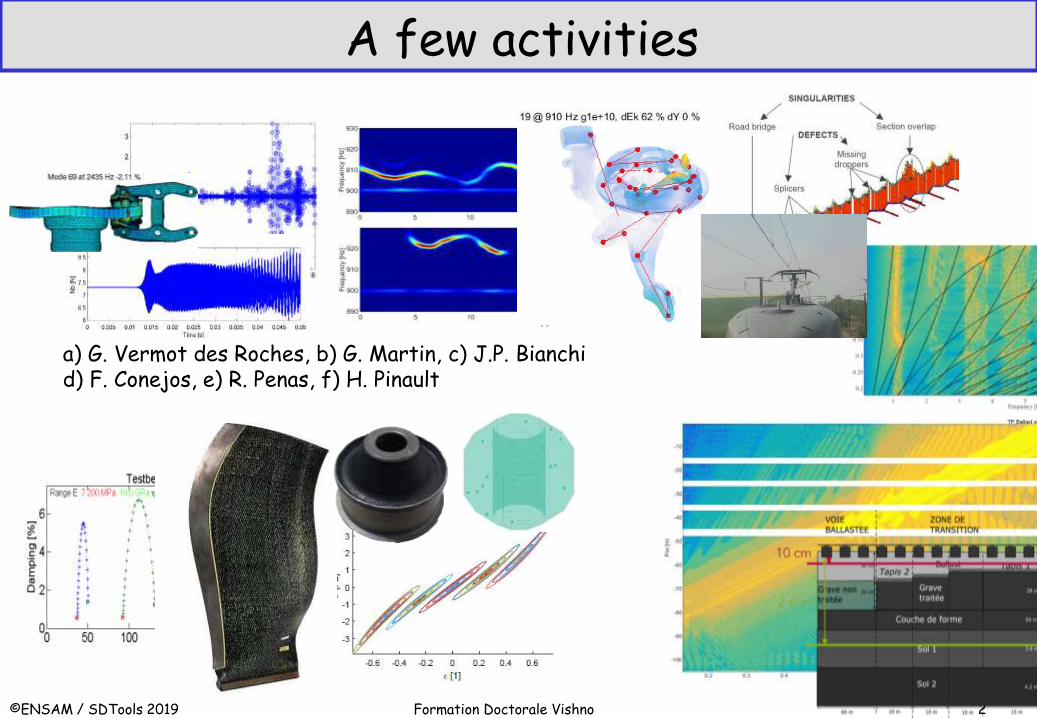
A few activities

©ENSAM / SDTools 2019 Formation Doctorale Vishno 2

Test 1

Test 2

a) G. Vermot des Roches, b) G. Martin, c) J.P. Bianchi d) F. Conejos, e) R. Penas, f) H. Pinault

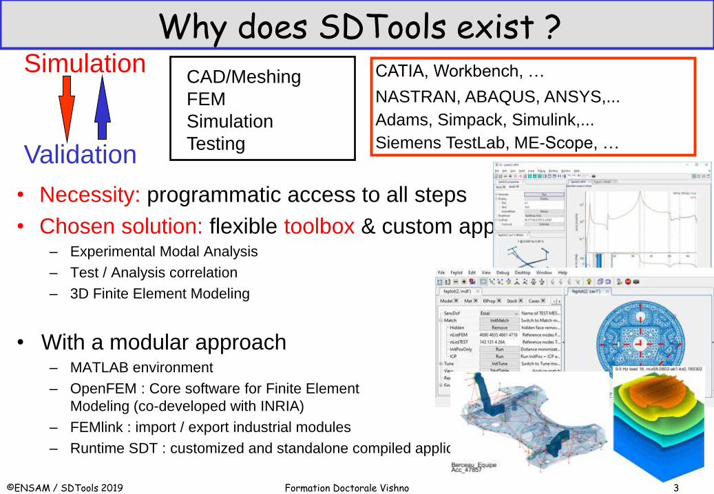
• Necessity: programmatic access to all steps

• Chosen solution: flexible toolbox & custom applications – Experimental Modal Analysis

– Test / Analysis correlation

– 3D Finite Element Modeling

• With a modular approach – MATLAB environment

– OpenFEM : Core software for Finite Element

Modeling (co-developed with INRIA)

– FEMlink : import / export industrial modules

– Runtime SDT : customized and standalone compiled applications

Why does SDTools exist ?


CAD/Meshing

FEM

Simulation

Testing

CATIA, Workbench, …

NASTRAN, ABAQUS, ANSYS,...

Adams, Simpack, Simulink,...

Siemens TestLab, ME-Scope, …

Simulation

Validation

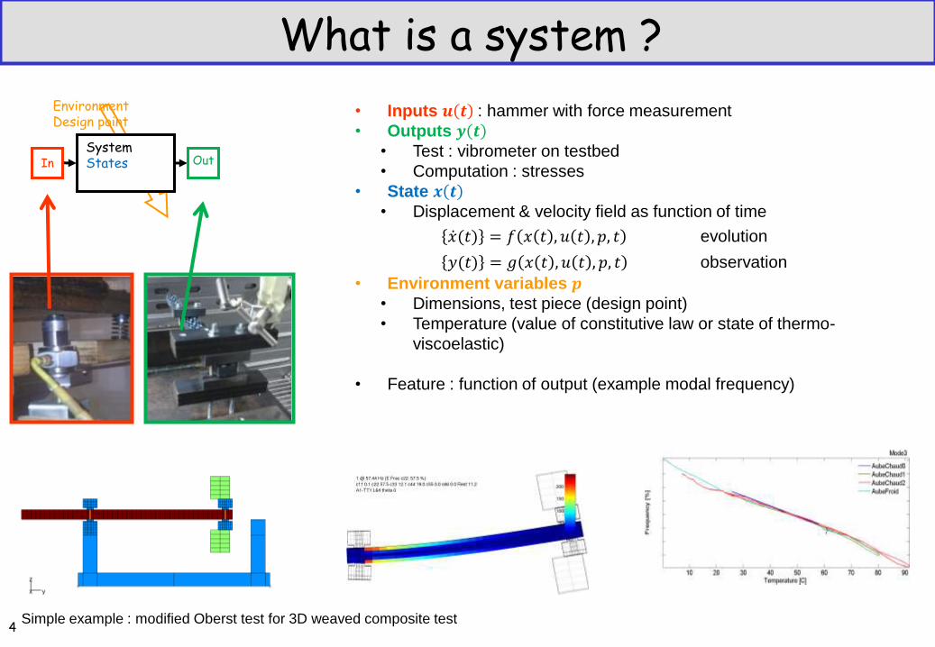
What is a system ?

In Out

Environment Design point

System States

Simple example : modified Oberst test for 3D weaved composite test

• Inputs 𝒖 𝒕 : hammer with force measurement

• Outputs 𝒚 𝒕

• Test : vibrometer on testbed

• Computation : stresses • State 𝒙 𝒕

• Displacement & velocity field as function of time

𝑥 (𝑡) = 𝑓 𝑥 𝑡 , 𝑢 𝑡 , 𝑝, 𝑡 evolution

𝑦(𝑡) = 𝑔 𝑥 𝑡 , 𝑢 𝑡 , 𝑝, 𝑡 observation

• Environment variables 𝒑

• Dimensions, test piece (design point)

• Temperature (value of constitutive law or state of thermo-

viscoelastic)

• Feature : function of output (example modal frequency)

4

5

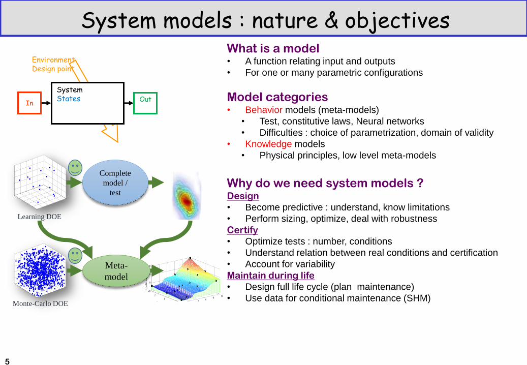
What is a model • A function relating input and outputs

• For one or many parametric configurations

Model categories • Behavior models (meta-models)

• Test, constitutive laws, Neural networks

• Difficulties : choice of parametrization, domain of validity

• Knowledge models

• Physical principles, low level meta-models

Why do we need system models ? Design

• Become predictive : understand, know limitations

• Perform sizing, optimize, deal with robustness

Certify

• Optimize tests : number, conditions

• Understand relation between real conditions and certification

• Account for variability

Maintain during life

• Design full life cycle (plan maintenance)

• Use data for conditional maintenance (SHM) 0

24

68

10

-2

0

2

-20

0

20

40

Parameter 1

Parameter 2

Healt

h i

nd

icato

r

Meta-

model

Complete

model /

test

Learning DOE

Monte-Carlo DOE

System models : nature & objectives

In Out


System States

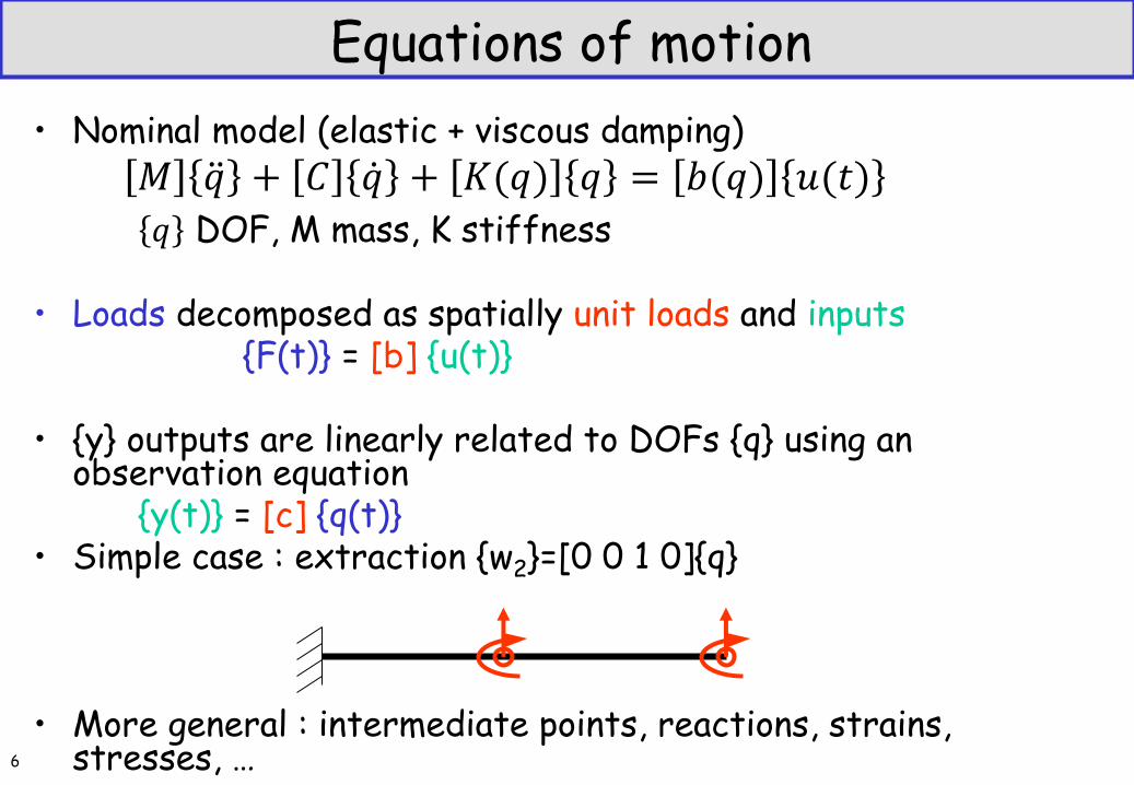
• Nominal model (elastic + viscous damping)

𝑀 𝑞 + 𝐶 𝑞 + 𝐾(𝑞) 𝑞 = 𝑏(𝑞) 𝑢(𝑡) 𝑞 DOF, M mass, K stiffness

• Loads decomposed as spatially unit loads and inputs {F(t)} = [b] {u(t)} • {y} outputs are linearly related to DOFs {q} using an

observation equation {y(t)} = [c] {q(t)} • Simple case : extraction {w2}=[0 0 1 0]{q}

• More general : intermediate points, reactions, strains, stresses, …

Equations of motion

6

Equations of motion

7

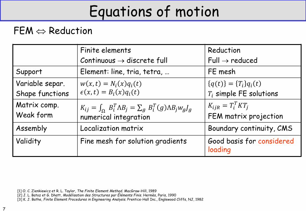
Finite elements

Continuous discrete full

Reduction

Full reduced

Support Element: line, tria, tetra, … FE mesh

Variable separ.

Shape functions

𝑤 𝑥, 𝑡 = 𝑁𝑖 𝑥 𝑞𝑖(𝑡) 𝜖 𝑥, 𝑡 = 𝐵𝑖 𝑥 𝑞𝑖(𝑡)

𝑞(𝑡) = 𝑇𝑖 𝑞𝑖 𝑡

𝑇𝑖 simple FE solutions

Matrix comp.

Weak form 𝐾𝑖𝑗 = 𝐵𝑖

𝑇Λ𝐵𝑗Ω= 𝐵𝑖

𝑇 𝑔 Λ𝐵𝑗𝑤𝑔𝐽𝑔𝑔

numerical integration

𝐾𝑖𝑗𝑅 = 𝑇𝑖𝑇𝐾𝑇𝑗

FEM matrix projection

Assembly Localization matrix Boundary continuity, CMS

Validity Fine mesh for solution gradients Good basis for considered loading

FEM Reduction

[1] O. C. Zienkiewicz et R. L. Taylor, The Finite Element Method. MacGraw-Hill, 1989 [2] J. L. Batoz et G. Dhatt, Modélisation des Structures par Éléments Finis. Hermès, Paris, 1990 [3] K. J. Bathe, Finite Element Procedures in Engineering Analysis. Prentice-Hall Inc., Englewood Cliffs, NJ, 1982

Ritz/Galerkin reduction from full


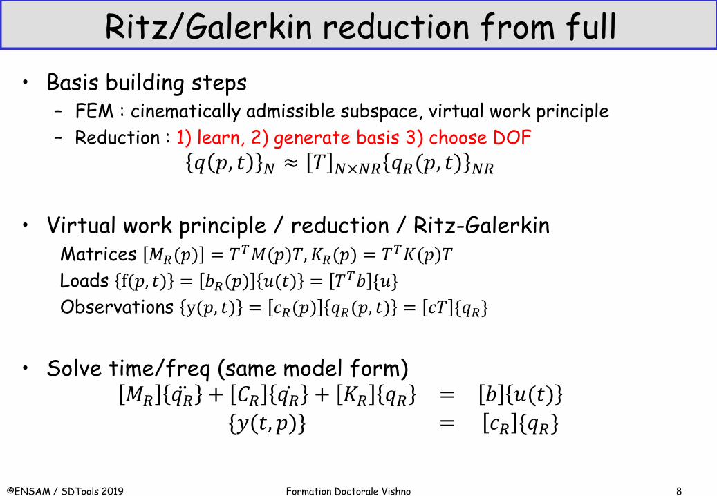
• Basis building steps – FEM : cinematically admissible subspace, virtual work principle

– Reduction : 1) learn, 2) generate basis 3) choose DOF

𝑞 𝑝, 𝑡 𝑁 ≈ 𝑇 𝑁×𝑁𝑅 𝑞𝑅(𝑝, 𝑡) 𝑁𝑅

• Virtual work principle / reduction / Ritz-Galerkin Matrices 𝑀𝑅(𝑝) = 𝑇𝑇𝑀(𝑝)𝑇, 𝐾𝑅(𝑝) = 𝑇𝑇𝐾(𝑝)𝑇

Loads f(𝑝, 𝑡) = 𝑏𝑅(𝑝) 𝑢(𝑡) = 𝑇𝑇𝑏 {𝑢}

Observations y(𝑝, 𝑡) = 𝑐𝑅(𝑝) 𝑞𝑅(𝑝, 𝑡) = 𝑐𝑇 {𝑞𝑅}

• Solve time/freq (same model form) 𝑀𝑅 𝑞𝑅 + 𝐶𝑅 𝑞𝑅 + 𝐾𝑅 𝑞𝑅 = 𝑏 𝑢(𝑡)

{𝑦(𝑡, 𝑝)} = 𝑐𝑅 {𝑞𝑅}

Outline : solvers for dynamics

Continuous/discrete/reduced models (a brief reminder)

Full order model solvers

• Direct frequency resolution

• Direct time integration (implicit/explicit, first/second order, Newmark, … Gaël Chevallier)

Reduced order model + time/frequency resolution

• Basic reduction : modal superposition, static correction, Guyan, Craig-Bampton, …

• Modern vision of reduction: learning phase, basis building, DOF choice

• Substructuring

• Parametric model reduction, error control

When does reduction become useful ?

Basic building blocks ? 9

MATLAB Tutorial : direct frequency response issues

• Step1 : assembly, sparse matrices

• Step 2 : point load, collocated displacement, factorization strategies

• Step 3 : subspace around resonance, phase collinearity, SVD

• Step 4 : Rayleigh-Ritz, reduced FRF


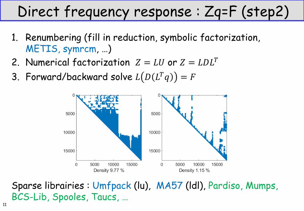
Direct frequency response : Zq=F (step2)

1. Renumbering (fill in reduction, symbolic factorization, METIS, symrcm, …)

2. Numerical factorization 𝑍 = 𝐿𝑈 or 𝑍 = 𝐿𝐷𝐿𝑇

3. Forward/backward solve 𝐿 𝐷 𝐿𝑇𝑞 = 𝐹

Sparse librairies : Umfpack (lu), MA57 (ldl), Pardiso, Mumps, BCS-Lib, Spooles, Taucs, …

11

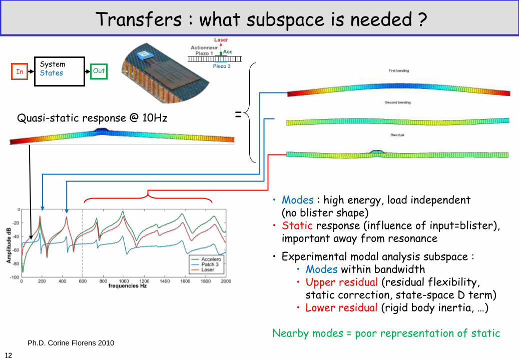
Transfers : what subspace is needed ?

12

• Experimental modal analysis subspace : • Modes within bandwidth • Upper residual (residual flexibility,

static correction, state-space D term) • Lower residual (rigid body inertia, …)

Nearby modes = poor representation of static

Ph.D. Corine Florens 2010

In Out System States

Quasi-static response @ 10Hz =

• Modes : high energy, load independent (no blister shape)

• Static response (influence of input=blister), important away from resonance

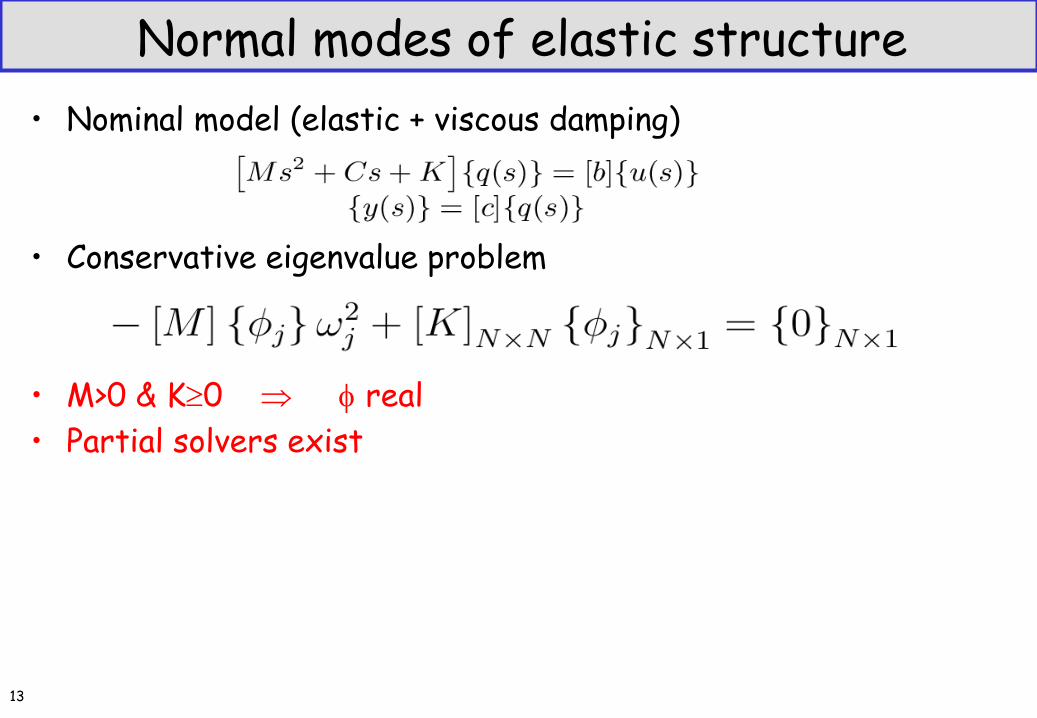
• Nominal model (elastic + viscous damping)

• Conservative eigenvalue problem

• M>0 & K0 real

• Partial solvers exist

Normal modes of elastic structure

13

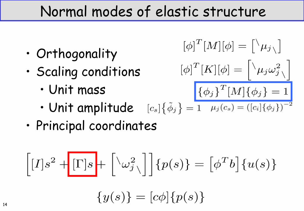
Normal modes of elastic structure

• Orthogonality

• Scaling conditions

• Unit mass

• Unit amplitude

• Principal coordinates

14

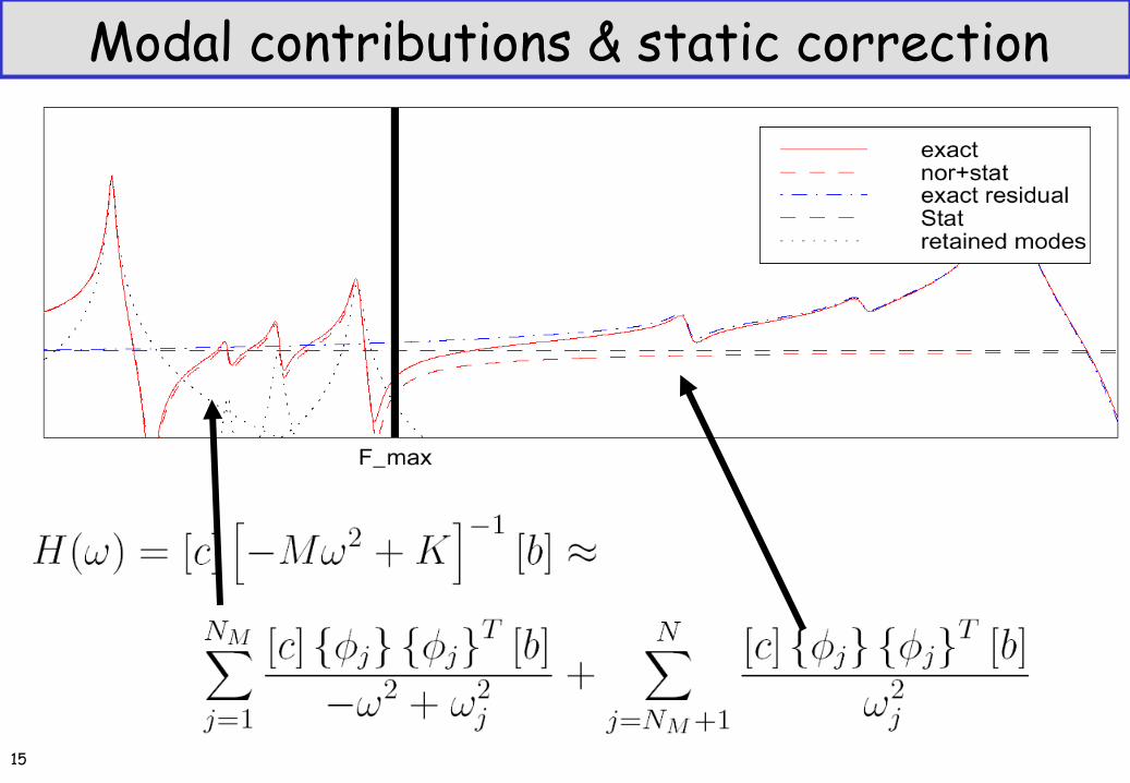
Modal contributions & static correction

15

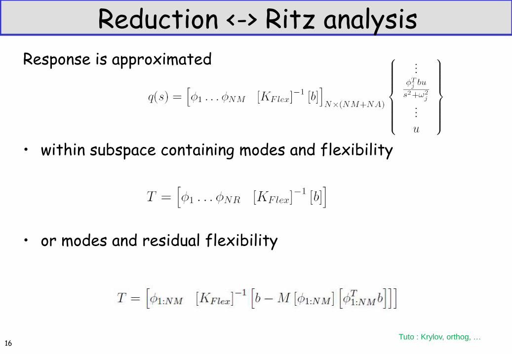
Reduction <-> Ritz analysis

Response is approximated

• within subspace containing modes and flexibility

• or modes and residual flexibility

16

Tuto : Krylov, orthog, …

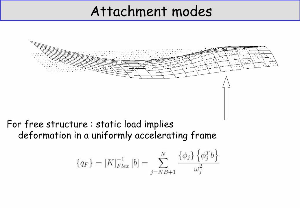
Attachment modes

For free structure : static load implies deformation in a uniformly accelerating frame

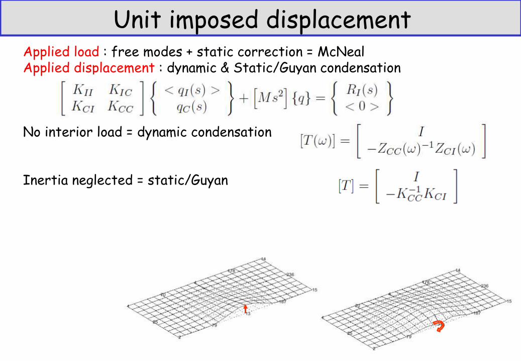
Applied load : free modes + static correction = McNeal Applied displacement : dynamic & Static/Guyan condensation No interior load = dynamic condensation Inertia neglected = static/Guyan

Unit imposed displacement

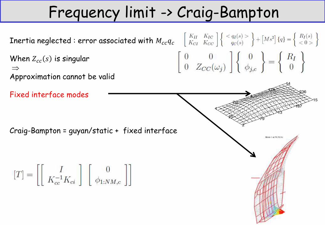
Frequency limit -> Craig-Bampton

Inertia neglected : error associated with 𝑀𝑐𝑐𝑞𝑐 When 𝑍𝑐𝑐 𝑠 is singular Approximation cannot be valid Fixed interface modes Craig-Bampton = guyan/static + fixed interface

19

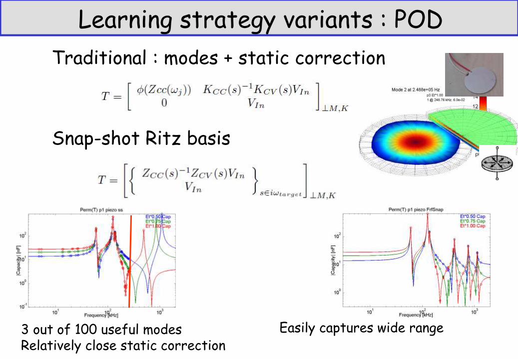
Learning strategy variants : POD

Traditional : modes + static correction

Snap-shot Ritz basis

3 out of 100 useful modes Relatively close static correction

Easily captures wide range

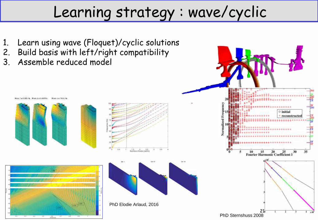
Learning strategy : wave/cyclic

1. Learn using wave (Floquet)/cyclic solutions 2. Build basis with left/right compatibility 3. Assemble reduced model

PhD Sternshuss 2008 21

PhD Elodie Arlaud, 2016

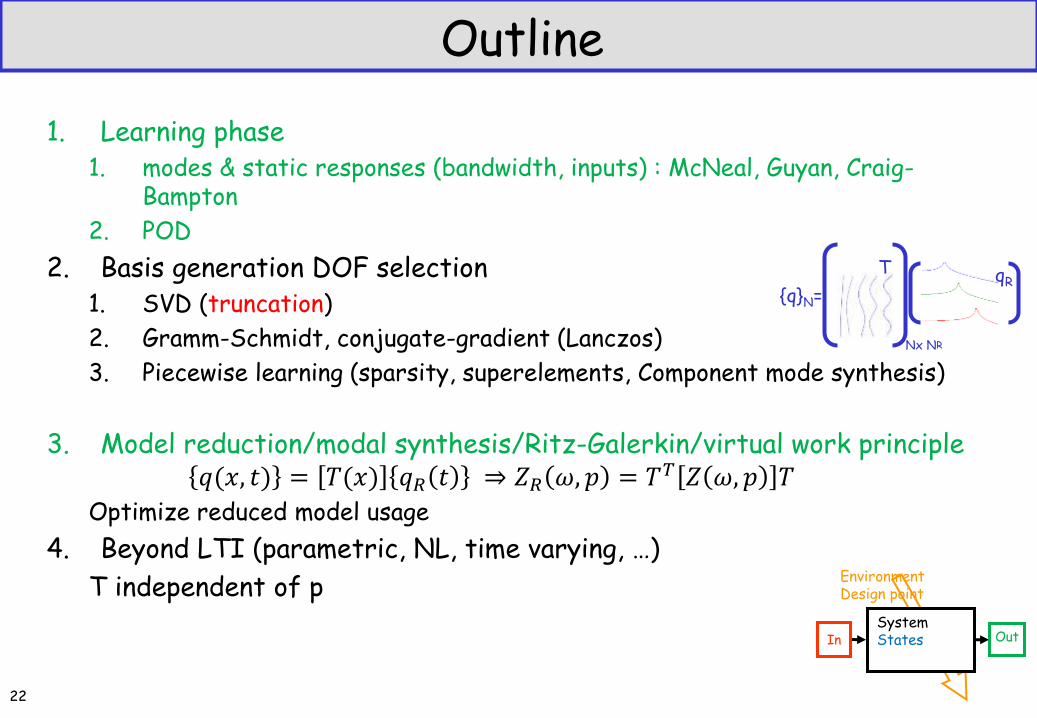
Outline

1. Learning phase 1. modes & static responses (bandwidth, inputs) : McNeal, Guyan, Craig-

Bampton

2. POD

2. Basis generation DOF selection 1. SVD (truncation)

2. Gramm-Schmidt, conjugate-gradient (Lanczos)

3. Piecewise learning (sparsity, superelements, Component mode synthesis)

3. Model reduction/modal synthesis/Ritz-Galerkin/virtual work principle 𝑞(𝑥, 𝑡) = 𝑇(𝑥) 𝑞𝑅 𝑡 ⇒ 𝑍𝑅 𝜔, 𝑝 = 𝑇𝑇 𝑍 𝜔, 𝑝 𝑇

Optimize reduced model usage

4. Beyond LTI (parametric, NL, time varying, …)

T independent of p

22

{q}N= qR

Nx NR

T

In Out


System States

Tuto steps 3-4

• POD learning

• Rayleigh-Ritz / reduced solve


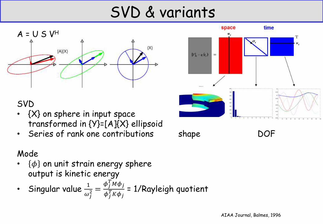
SVD & variants A = U S VH

SVD • {X} on sphere in input space

transformed in {Y}=[A]{X} ellipsoid • Series of rank one contributions shape DOF

Mode • 𝜙 on unit strain energy sphere

output is kinetic energy

• Singular value 1

𝜔𝑗2 =

𝜙𝑗𝑇𝑀𝜙𝑗

𝜙𝑗𝑇𝐾𝜙𝑗

= 1/Rayleigh quotient

AIAA Journal, Balmes, 1996

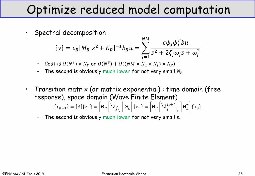
Optimize reduced model computation

• Spectral decomposition

𝑦 = 𝑐𝑅 𝑀𝑅 𝑠2+ 𝐾𝑅

−1𝑏𝑅𝑢 = 𝑐𝜙𝑗𝜙𝑗

𝑇𝑏𝑢

𝑠2 + 2𝜁𝑗𝜔𝑗𝑠 + 𝜔𝑗2

𝑁𝑀

𝑗=1

– Cost is 𝑂 𝑁3 × 𝑁𝐹 or 𝑂 𝑁3 + 𝑂 (𝑁𝑀 ×𝑁𝑎 × 𝑁𝑠) × 𝑁𝐹

– The second is obviously much lower for not very small 𝑁𝐹

• Transition matrix (or matrix exponential) : time domain (free response), space domain (Wave Finite Element)

𝑥𝑛+1 = 𝐴 𝑥𝑛 = Θ𝑅 𝜆𝑗\

\ Θ𝐿𝑇 𝑥𝑛 = Θ𝑅 𝜆𝑗

𝑛+1\\ Θ𝐿𝑇 𝑥0

– The second is obviously much lower for not very small 𝑛


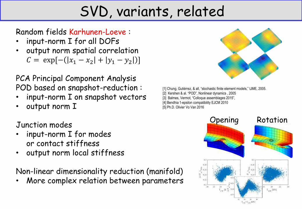
SVD, variants, related Random fields Karhunen-Loeve : • input-norm I for all DOFs • output norm spatial correlation

𝐶 = exp[− 𝑥1 − 𝑥2 + 𝑦1 − 𝑦2 ]

PCA Principal Component Analysis POD based on snapshot-reduction : • input-norm I on snapshot vectors • output norm I

Junction modes • input-norm I for modes

or contact stiffness • output norm local stiffness

Non-linear dimensionality reduction (manifold) • More complex relation between parameters

[1] Chung, Gutiérrez, & all, “stochastic finite element models,” IJME, 2005.

[2] Kershen & al. “POD”, Nonlinear dynamics , 2005

[3] Balmes, Vermot, “Colloque assemblages 2015”,

[4] Bendhia 1-epsilon compatibility EJCM 2010

[5] Ph.D. Olivier Vo Van 2016

Opening Rotation

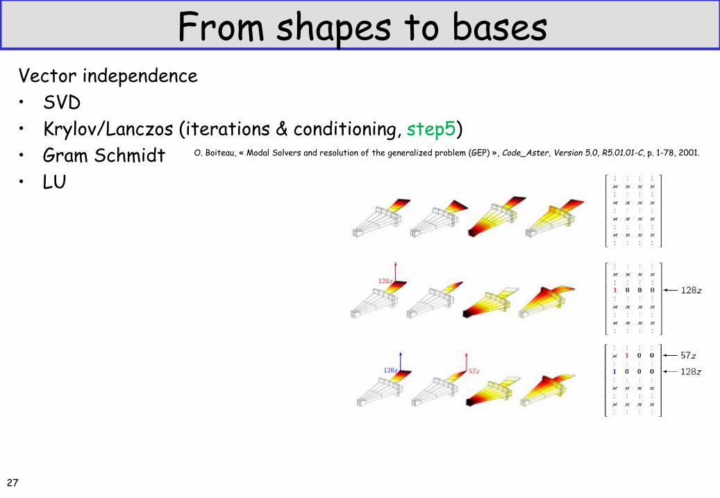
From shapes to bases Vector independence

• SVD

• Krylov/Lanczos (iterations & conditioning, step5)

• Gram Schmidt

• LU

27

O. Boiteau, « Modal Solvers and resolution of the generalized problem (GEP) », Code_Aster, Version 5.0, R5.01.01-C, p. 1-78, 2001.

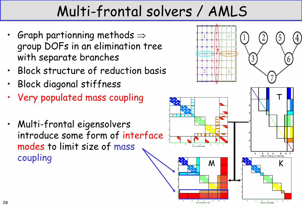
Multi-frontal solvers / AMLS

• Graph partionning methods group DOFs in an elimination tree with separate branches

• Block structure of reduction basis

• Block diagonal stiffness

• Very populated mass coupling

• Multi-frontal eigensolvers introduce some form of interface modes to limit size of mass coupling

K M

28

T

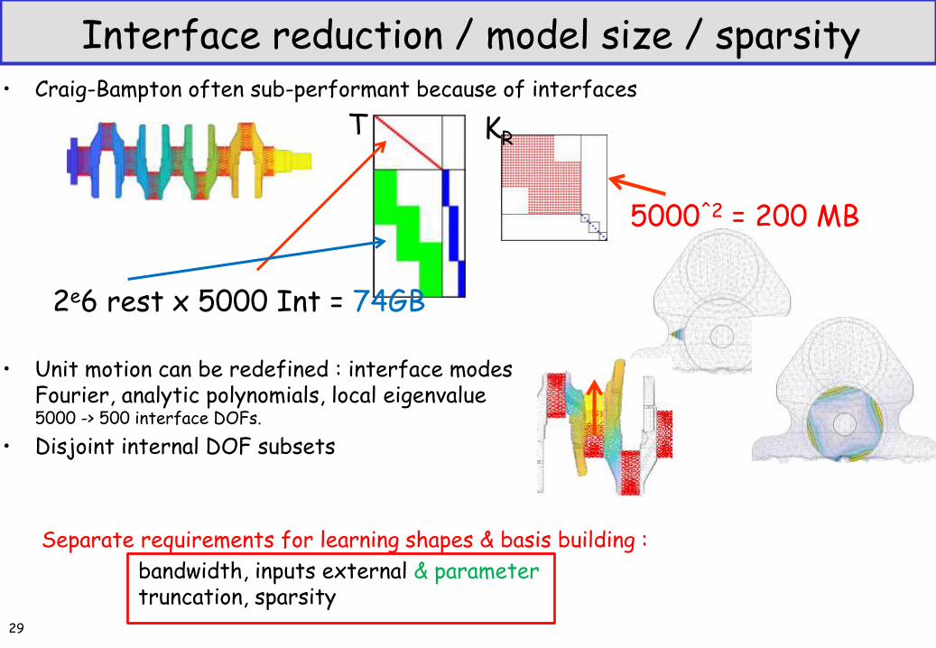
• Craig-Bampton often sub-performant because of interfaces

• Unit motion can be redefined : interface modes

Fourier, analytic polynomials, local eigenvalue 5000 -> 500 interface DOFs.

• Disjoint internal DOF subsets

Separate requirements for learning shapes & basis building :

bandwidth, inputs external & parameter truncation, sparsity

T

Interface reduction / model size / sparsity

2e6 rest x 5000 Int = 74GB

5000^2 = 200 MB

KR

29

MATLAB Tutorial : reduction, full operators

• Step 5 : Krylov

• Step 6 : sparse reduced model

• Step 7 : frequency limit CB

• Step 8 : an experimental case of SVD


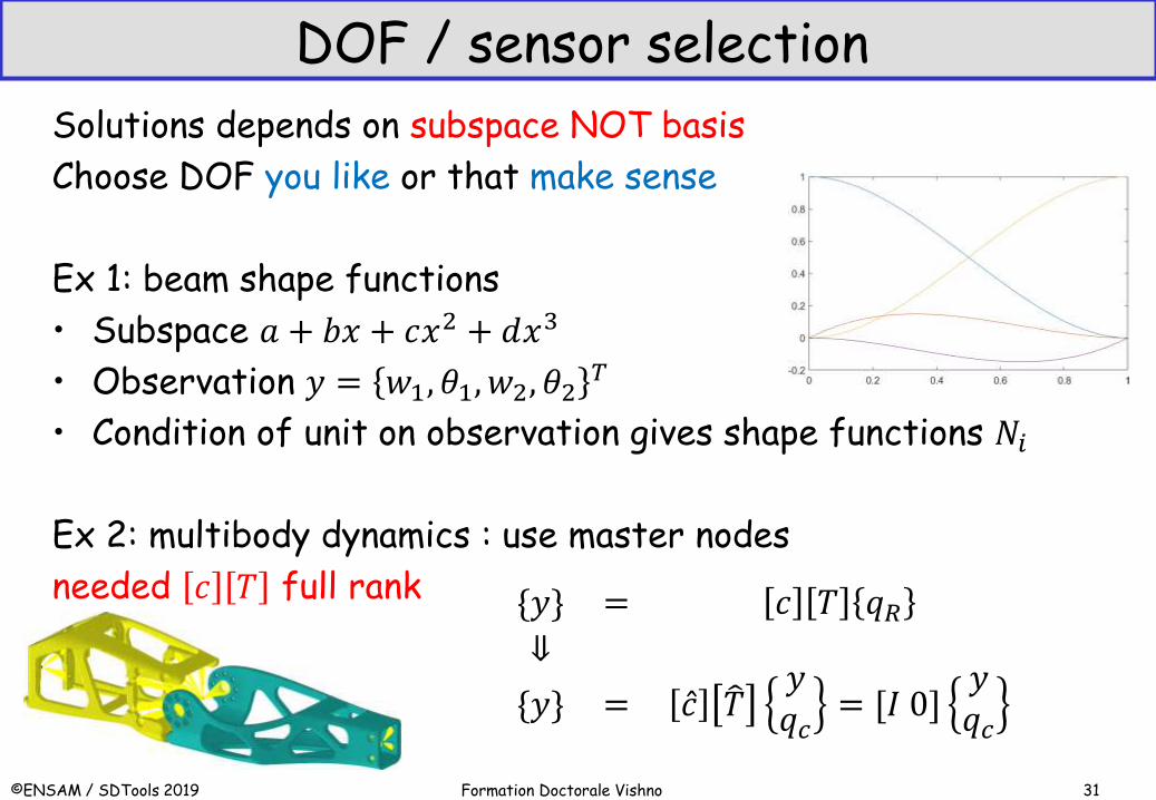
DOF / sensor selection

Solutions depends on subspace NOT basis

Choose DOF you like or that make sense

Ex 1: beam shape functions

• Subspace 𝑎 + 𝑏𝑥 + 𝑐𝑥2 + 𝑑𝑥3

• Observation 𝑦 = 𝑤1, 𝜃1, 𝑤2, 𝜃2𝑇

• Condition of unit on observation gives shape functions 𝑁𝑖

Ex 2: multibody dynamics : use master nodes

needed 𝑐 𝑇 full rank


{𝑦} = 𝑐 𝑇 𝑞𝑅⇓

{𝑦} = 𝑐 𝑇 𝑦𝑞𝑐

= [𝐼 0]𝑦𝑞𝑐

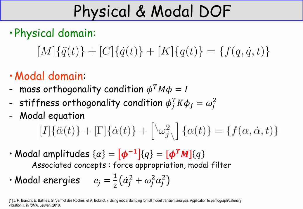
Physical & Modal DOF

•Physical domain:

•Modal domain: - mass orthogonality condition 𝜙𝑇𝑀𝜙 = 𝐼

- stiffness orthogonality condition 𝜙𝑗𝑇𝐾𝜙𝑗 = 𝜔𝑗

2

- Modal equation

• Modal amplitudes 𝛼 = 𝝓−𝟏 𝑞 = 𝝓𝑻𝑴 𝑞 Associated concepts : force appropriation, modal filter

• Modal energies 𝑒𝑗 =1

2𝛼 𝑗2 +𝜔𝑗

2𝛼𝑗2

[1] J. P. Bianchi, E. Balmes, G. Vermot des Roches, et A. Bobillot, « Using modal damping for full model transient analysis. Application to pantograph/catenary

vibration », in ISMA, Leuven, 2010.

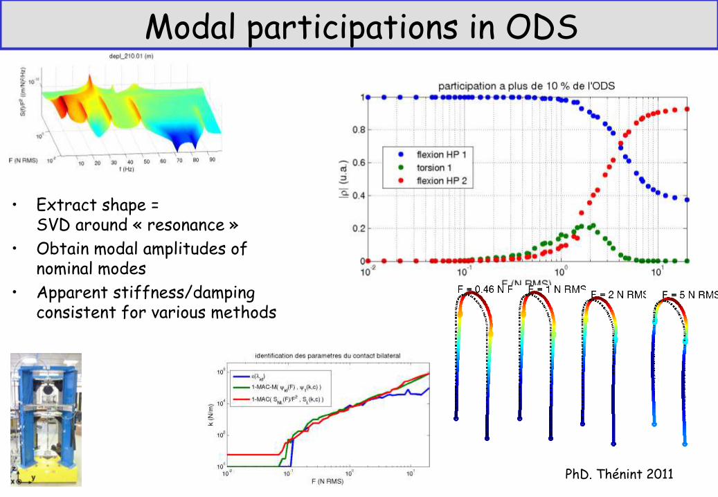
Modal participations in ODS

• Extract shape = SVD around « resonance »

• Obtain modal amplitudes of nominal modes

• Apparent stiffness/damping consistent for various methods

PhD. Thénint 2011

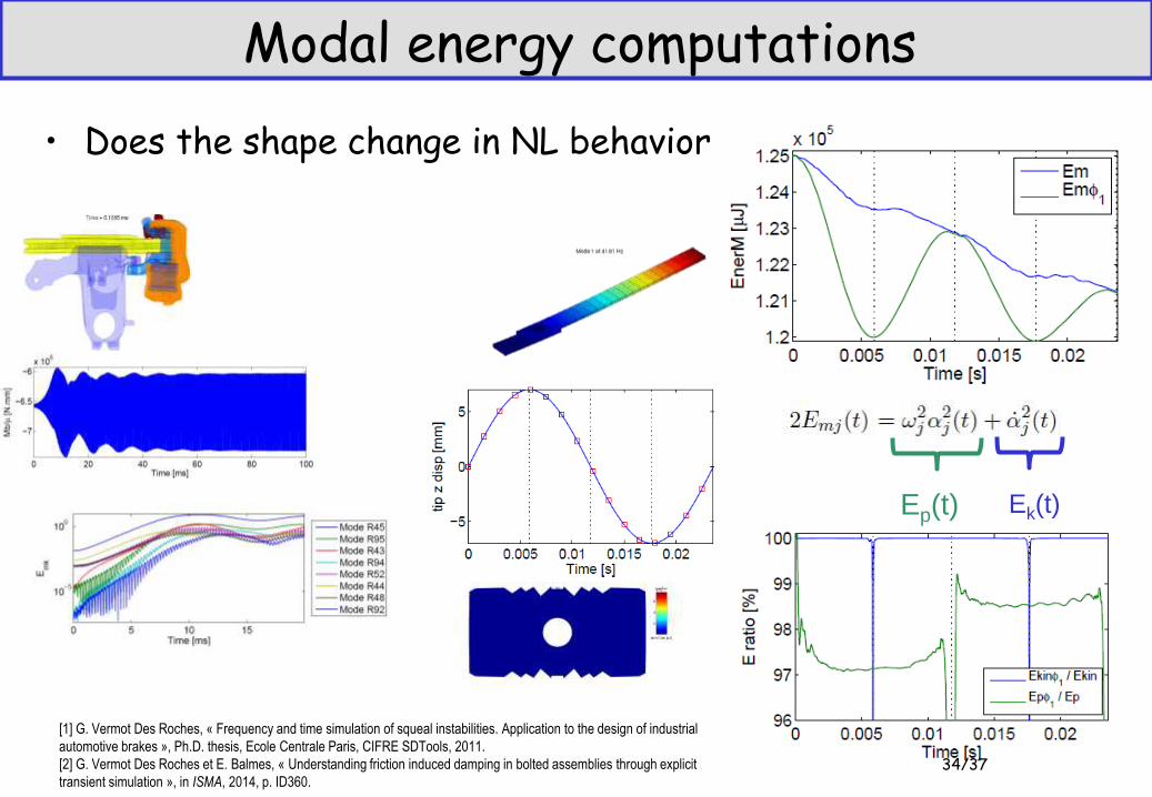
Modal energy computations

• Does the shape change in NL behavior

Ep(t) Ek(t)

34/37

[1] G. Vermot Des Roches, « Frequency and time simulation of squeal instabilities. Application to the design of industrial

automotive brakes », Ph.D. thesis, Ecole Centrale Paris, CIFRE SDTools, 2011.

[2] G. Vermot Des Roches et E. Balmes, « Understanding friction induced damping in bolted assemblies through explicit

transient simulation », in ISMA, 2014, p. ID360.

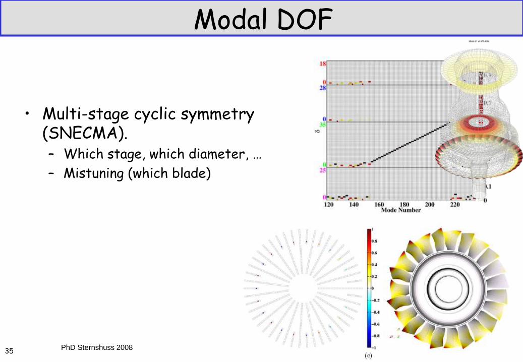
Modal DOF

• Multi-stage cyclic symmetry (SNECMA). – Which stage, which diameter, …

– Mistuning (which blade)

35 PhD Sternshuss 2008

36

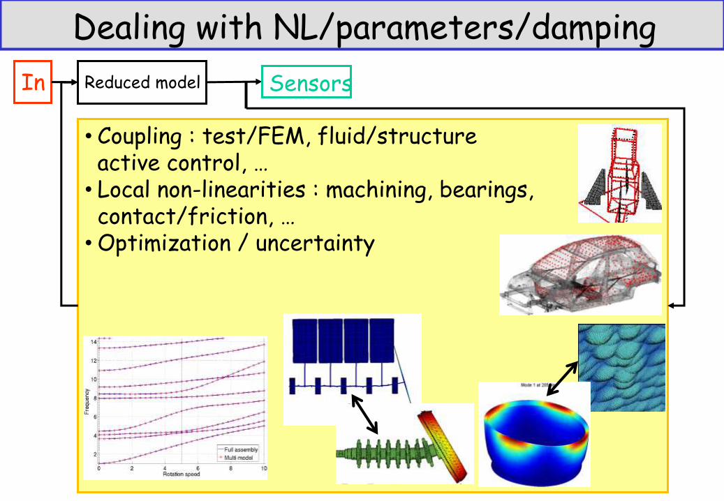
Dealing with NL/parameters/damping

Reduced model

• Coupling : test/FEM, fluid/structure active control, …

• Local non-linearities : machining, bearings, contact/friction, …

• Optimization / uncertainty

In Sensors

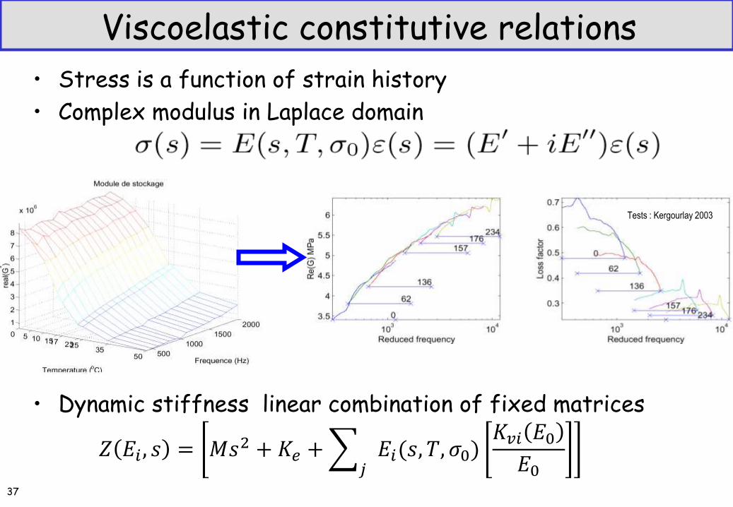
Viscoelastic constitutive relations

• Stress is a function of strain history

• Complex modulus in Laplace domain

• Dynamic stiffness linear combination of fixed matrices

𝑍 𝐸𝑖 , 𝑠 = 𝑀𝑠2 + 𝐾𝑒 + 𝐸𝑖(𝑠, 𝑇, 𝜎0)𝐾𝑣𝑖 𝐸0𝐸0𝑗

Tests : Kergourlay 2003

37

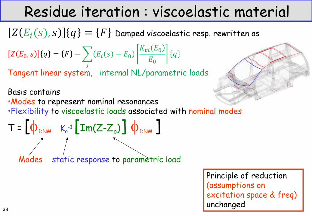
𝑍 𝐸𝑖(𝑠), 𝑠 𝑞 = 𝐹 Damped viscoelastic resp. rewritten as

𝑍 𝐸0, 𝑠 𝑞 = 𝐹 − 𝐸𝑖 𝑠 − 𝐸0𝐾𝑣𝑖 𝐸0𝐸0

𝑗

𝑞

Tangent linear system, internal NL/parametric loads Basis contains •Modes to represent nominal resonances •Flexibility to viscoelastic loads associated with nominal modes

T = [1:NM Ko-1 [Im(Z-Zo)] 1:NM ]

Residue iteration : viscoelastic material

Modes static response to parametric load

Principle of reduction (assumptions on excitation space & freq) unchanged

38

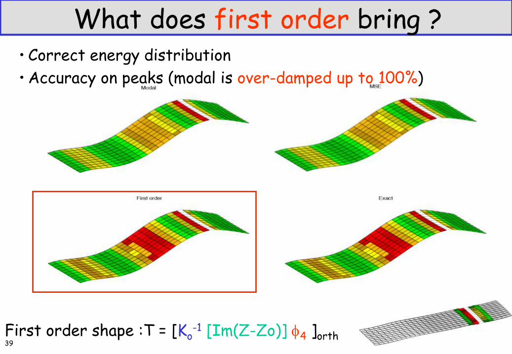
What does first order bring ? • Correct energy distribution

• Accuracy on peaks (modal is over-damped up to 100%)

First order shape :T = [Ko-1 [Im(Z-Zo)] 4 ]orth

39

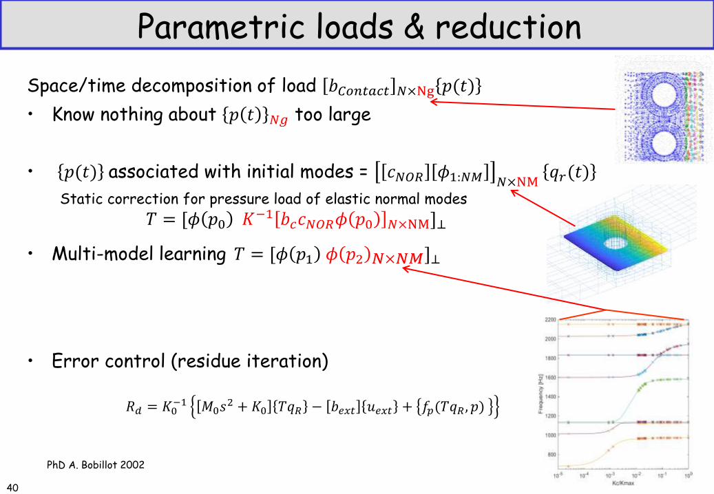
Parametric loads & reduction

Space/time decomposition of load 𝑏𝐶𝑜𝑛𝑡𝑎𝑐𝑡 𝑁×Ng 𝑝(𝑡)

• Know nothing about 𝑝 𝑡 𝑁𝑔 too large

• 𝑝(𝑡) associated with initial modes = 𝑐𝑁𝑂𝑅 𝜙1:𝑁𝑀 𝑁×NM 𝑞𝑟(𝑡)

Static correction for pressure load of elastic normal modes

𝑇 = [𝜙 𝑝0 𝐾−1 𝑏𝑐𝑐𝑁𝑂𝑅𝜙 𝑝0 𝑁×NM]⊥

• Multi-model learning 𝑇 = [𝜙 𝑝1 𝜙 𝑝2 𝑁×𝑁𝑀]⊥

• Error control (residue iteration)

𝑅𝑑 = 𝐾0−1 𝑀0𝑠

2 + 𝐾0 𝑇𝑞𝑅 − 𝑏𝑒𝑥𝑡 𝑢𝑒𝑥𝑡 + 𝑓𝑝(𝑇𝑞𝑅 , 𝑝)

40

PhD A. Bobillot 2002

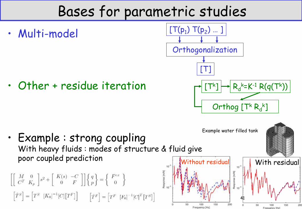
• Multi-model

• Other + residue iteration

• Example : strong coupling With heavy fluids : modes of structure & fluid give poor coupled prediction

Bases for parametric studies

Example water filled tank

With residual Without residual

[T(p1) T(p2) … ]

Orthogonalization

[T]

[Tk] Rdk=K-1 R(q(Tk))

Orthog [Tk Rdk]

41

MATLAB/SDT TutoParametric

• Step 1 : Load model

• Step 2 : Multi-model reduction

• Step 3 : Analyze frequency/damping evolution

• Step 4 : Analyze MAC, use modal coordinates


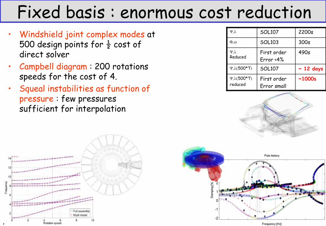
Fixed basis : enormous cost reduction

43

• Windshield joint complex modes at 500 design points for ½ cost of direct solver

• Campbell diagram : 200 rotations speeds for the cost of 4.

• Squeal instabilities as function of pressure : few pressures sufficient for interpolation

Y,l SOL107 2200s

F,w SOL103 300s

Y,l Reduced

First order

Error <4%

490s

Y,l(500*T) SOL107 ~ 12 days

Y,l(500*T)

reduced

First order

Error small

~1000s

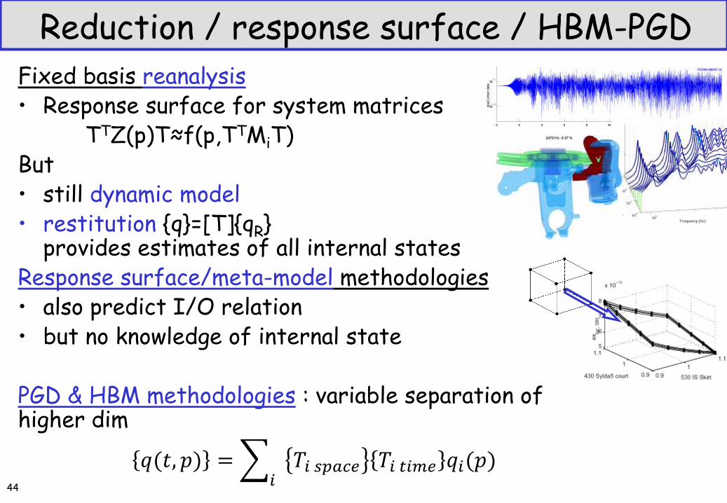
Reduction / response surface / HBM-PGD Fixed basis reanalysis • Response surface for system matrices TTZ(p)T≈f(p,TTMiT) But • still dynamic model • restitution {q}=[T]{qR}

provides estimates of all internal states Response surface/meta-model methodologies • also predict I/O relation • but no knowledge of internal state

PGD & HBM methodologies : variable separation of higher dim

𝑞(𝑡, 𝑝) = 𝑇𝑖 𝑠𝑝𝑎𝑐𝑒 𝑇𝑖 𝑡𝑖𝑚𝑒 𝑞𝑖(𝑝)𝑖

44

Conclusions : solvers for dynamics

Continuous/discrete/reduced models (a brief reminder)

Full order model solvers

• Direct frequency resolution

• Direct time integration (implicit/explicit, first/second order, Newmark, … Gaël Chevallier)

Reduced order model + time/frequency resolution

• Basic reduction : modal superposition, static correction, Guyan, Craig-Bampton, …

• Modern vision of reduction: learning phase, basis building, DOF choice

• Substructuring

• Parametric model reduction, error control

https://savoir.ensam.eu/moodle/course/search.php?search=1874 ©ENSAM / SDTools 2019 Formation Doctorale Vishno 45

Documents

Simulations numériques pour la dynamique Réduction de modèle