NUMERICAL SIMULATIONS AND PREDICTIVE MODELS OF UNDRAINED

PENETRATION IN SOFT SOILS

A Dissertation

by

HAN SHI

Submitted to the Office of Graduate Studies of

Texas A&M University in partial fulfillment of the requirements for the degree of

DOCTOR OF PHILOSOPHY

August 2005

Major Subject: Civil Engineering

NUMERICAL SIMULATIONS AND PREDICTIVE MODELS OF UNDRAINED

PENETRATION IN SOFT SOILS

A Dissertation

by

HAN SHI

Submitted to the Office of Graduate Studies of

Texas A&M University in partial fulfillment of the requirements for the degree of

DOCTOR OF PHILOSOPHY

Approved by: Chair of Committee, Charles Aubeny Committee Members, James D. Murff J. N. Reddy Harry Hogan Head of Department, David Rosowsky

August 2005

Major Subject: Civil Engineering

iii

ABSTRACT

Numerical Simulations and Predictive Models of Undrained

Penetration in Soft Soils. (August 2005)

Han Shi, B.S., China University of Geosciences;

M.S., China University of Geosciences

Chair of Advisory Committee: Dr. Charles Aubeny

There are two aspects in this study: cylinder penetrations and XBP (Expendable

Bottom Penetrometer) interpretations. The cylinder studies firstly investigate the

relationship between the soil resisting force and penetration depth by a series of rate-

independent finite element analyses of pre-embedded penetration depths, and validate

the results by upper and lower bound solutions from classical plasticity theory.

Furthermore, strain rate effects are modeled by finite element simulations within a

framework of rate-dependent plasticity. With all forces acting on the cylinder estimated,

penetration depths are predicted from simple equations of motion for a single particle.

Comparisons to experimental results show reasonable agreement between model

predictions and measurements.

The XBP studies follow the same methodology in investigating the soil shearing

resistance as a function of penetration depth and velocity by finite element analyses.

With the measurements of time decelerations during penetration of the XBP, sediment

shear strength profile is inferred from a single particle kinetic model. The predictions

compare favorably with experimental measurements by vane shear tests.

iv

ACKNOWLEDGMENTS

This research was sponsored by the Office of Naval Research and its support is

gratefully acknowledged.

I would like to express my sincere gratitude to my advisor, Dr. Charles Aubeny,

for his invaluable guidance, encouragement and assistance throughout this research. It

was a pleasure and privilege working with him. I also greatly appreciate the tremendous

help from Dr. Don Murff during my study. I would also like to thank Dr. J. N. Reddy

and Dr. Harry Hogan for serving as the advisory committee.

I would like to extend my thanks to all my friends, and special thanks to Zhigang

Yao, for helping me on this research. Finally, I would like to thank my family for their

enduring love and support.

v

TABLE OF CONTENTS

Page ABSTRACT ..................................................................................................................... iii

ACKNOWLEDGMENTS.................................................................................................iv

TABLE OF CONTENTS ...................................................................................................v

LIST OF FIGURES........................................................................................................ viii

LIST OF TABLES ...........................................................................................................xii

CHAPTER

I INTRODUCTION ................................................................................................1

1.1 Scope of Study ...........................................................................................1 1.2 Objectives...................................................................................................5 1.3 Outline of Research....................................................................................5

II BACKGROUND ..................................................................................................7

2.1 Plasticity Concepts .....................................................................................7 2.2 Plastic Limit Methods ................................................................................9

2.2.1 Lower Bound Method .....................................................................10 2.2.2 Upper Bound Method......................................................................18 2.2.3 Plasticity Solutions for Fully Embedded Cylinder..........................24 2.2.4 Plasticity Solutions for Partially Embedded Cylinders ...................26

2.3 Finite Element Method.............................................................................35 2.3.1 FEM Theory ....................................................................................35 2.3.2 FEM Studies for Cylinders of Flow-around Conditions .................37

2.4 Rate Dependent Properties of Soil ...........................................................39 2.5 Experimental Studies................................................................................41

2.5.1 Miniature Vane Shear Tests ............................................................41 2.5.2 Penetration Tests .............................................................................43 2.5.3 XBP Tests........................................................................................46

III RATE-INDEPENDENT STUDIES....................................................................49

3.1 Plastic Limit Analysis ..............................................................................49 3.1.1 Lower Bound Analysis....................................................................49

vi

CHAPTER Page

3.1.2 Upper Bound Analysis for Variable Strength Profiles....................54 3.1.3 Upper Bound Analysis for Penetration Exceeding One Radius......59

3.2 Finite Element Analysis ...........................................................................64 3.2.1 Geometry Model .............................................................................64 3.2.2 Material Model ................................................................................65 3.2.3 Boundary Conditions.......................................................................66 3.2.4 Mesh Construction ..........................................................................69 3.2.5 Loading Step ...................................................................................71 3.2.6 Cylinder Penetration Studies...........................................................72 3.2.7 XBP Penetration Studies .................................................................74

3.3 Comparison of Solutions..........................................................................77

IV RATE-DEPENDENT STUDIES........................................................................89

4.1 Rate-Dependent Strength Model ..............................................................89 4.2 Finite Element Studies for Cylinders .......................................................91

4.2.1 Finite Element Model......................................................................92 4.2.2 Finite Element Results ....................................................................93 4.2.3 Empirical Resisting Force Relations ...............................................99

4.3 Finite Element Studies for XBPs ...........................................................102 4.4 Summary and Discussions .....................................................................102

V PREDICTIVE MODELS .................................................................................105

5.1 Penetration Studies.................................................................................105 5.1.1 Penetration Model .........................................................................105 5.1.2 Parametric Studies.........................................................................110 5.1.3 Rate-Dependent Strength and Sensitivity .....................................112 5.1.4 Comparison to Experimental Data ................................................117

5.2 XBP Interpretations................................................................................123 5.2.1 Algorithm for XBP Interpretation .................................................123 5.2.2 Field Measurements ......................................................................125 5.2.3 Interpreted Undrained Shear Strength Profiles .............................128

VI CONCLUSIONS AND RECOMMENDATIONS ..........................................140

6.1 Conclusions ............................................................................................140 6.2 Recommendations ..................................................................................144

REFERENCES...............................................................................................................146

vii

Page APPENDIX A MATLAB PROGRAM: MOC_CYLINDER .......................................151

APPENDIX B MATLAB PROGRAM: RH_CYLINDER...........................................157

APPENDIX C MATLAB PROGRAM: CU_CYLINDER...........................................170

APPENDIX D MATLAB PRGRAM: MINE_BURIAL ..............................................173

APPENDIX E MATLAB PROGRAM: XBP_SOFTCLAY ........................................177

APPENDIX F A TYPICAL ABAQUS INPUT FILE (GENERATED BY ABAQUS CAE) ...................................................180

VITA ..............................................................................................................................185

viii

LIST OF FIGURES

FIGURE Page

1.1 Definition Sketch of Penetrating Cylinder (after Aubeny and Shi, 2005a) .......3

1.2 Definition Sketch of Penetrating XBP (Aubeny and Shi, 2005b)......................4

2.1 Plastic Material Models......................................................................................8

2.2 Mohr’s Circle and Failure Condition (after Murff, 2003)................................10

2.3 Illustration of the Method of Characteristics....................................................13

2.4 Mapped Rectangular Grids of the Radial Fan (Murff, 2003)...........................16

2.5 Calculation of the Dissipation Rate for Slip Surfaces (after Murff, 2002) ......20

2.6 Failure Mechanism Developed from MOC......................................................22

2.7 The Resultant Velocity along OA ....................................................................22

2.8 Examples of Characteristic Nets by Randolph and Houlsby (1984)................25

2.9 Solution for Cylindrical (T-bar) Penetrometer (Randolph et al., 2000)...........25

2.10 Characteristic Net for Uniform Strength (after Murff et al., 1989)..................27

2.11 Upper Bound Models (Murff et al., 1989) .......................................................29

2.12 Comparison of Lower and Upper Bound Solutions (after Murff et al., 1989)...................................................................................34

2.13 FEM Solutions for Cylinders of Flow around Conditions (Yao, 2003)...........38

2.14 Normalized Shear Strength versus Strain Rate, CK0UC Tests, Resedimented BBC (Sheahan et al., 1996) ....................................................40

2.15 The Vane Shear Testing Machine Set-Up (Munim, 2003) ..............................42

2.16 Penetration Test Basin with Gulf of Mexico Sediments (Yao, 2003)..............44

2.17 Typical Time-Dependent Penetration for Non-Impact Tests (after Aubeny and Dunlap, 2003; Munim, 2003).............................................46

ix

FIGURE Page 2.18 Expendable Bottom Penetrometer, XBP (Aubeny and Shi, 2005b) ................47

2.19 Typical XBP Field Record (Stoll et al., 2004) .................................................48

3.1 Boundary Condition for the Method of Characteristics ...................................51

3.2 Effect of Strength Gradient on Characteristics Solution (Aubeny et al., 2005)........................................................................................53

3.3 Normalized Load Capacity from MOC Solutions (Aubeny et al., 2005) ........54

3.4 Extension of Randolph-Houlsby Solution (Aubeny et al., 2005) ....................59

3.5 Geometry Model for Full Flow-around Cylinder.............................................65

3.6 Boundary Conditions at the Soil-Cylinder Interface........................................67

3.7 Boundary Conditions of a Fully Embedded Cylinder (No Slippage) ..............68

3.8 Finite Element Mesh for Full Flow-around Cylinder.......................................70

3.9 Effect of Mesh Refinement on the Collapse Loads of a Full Flow-around Cylinder........................................................................71

3.10 Loading Step for a Fully Embedded Rough Cylinder......................................72

3.11 Finite Element Model for Cylinder Penetration Studies, h/D≤0.5 ...................73

3.12 Finite Element Model for Cylinder Penetration Studies, h/D>0.5...................74

3.13 Finite Element Model for the XBP Penetration Studies ..................................75

3.14 Influencing Factors of the Collapse Load for the Hard Layer Study ...............76

3.15 Collapse Loads for Cylinders of h/D≤0.5 and η=0 ..........................................79

3.16 Collapse Loads for Cylinders of h/D≤0.5 and η=∞ .........................................80

3.17 Collapse Loads for Cylinders of h/D>0.5 and η=0 ..........................................82

3.18 Collapse Loads for Cylinders of h/D>0.5 and η=∞ .........................................83

x

FIGURE Page

3.19 Empirical Curve Fits ........................................................................................85

3.20 Collapse Loads for the XBP Penetration..........................................................87

3.21 Preliminary Hard Layer Study Results.............................................................88

4.1 Rate-Dependent Strength Model ......................................................................90

4.2 Stress Profile ahead of Cylinder at Various Penetration Velocities.................94

4.3 Finite Element Predictions of Collapse Loads at Various Velocities ..............96

4.4 Comparison of Strain Rate Multipliers λ0 and ρ0 .............................................96

4.5 Simplified Prediction of Strain Rate Effects (Rough, η = 0 ) ..........................97

4.6 Simplified Prediction of Strain Rate Effects (Smooth, η = 0 ) ........................98

4.7 Simpified Prediction of Strain Rate Effects (Rough, η = ∞ )...........................98

4.8 Simplified Prediction of Strain Rate Effects (Smooth, η = ∞ ).......................99

4.9 Evaluation of Empirical Estimates of Collapse Loads (Rough, η = 0 ) .........100

4.10 Evaluation of Empirical Estimates of Collapse Loads (Smooth, η = 0 ) .......100

4.11 Evaluation of Empirical Estimates of Collapse Loads (Rough, η = ∞ ) ........101

4.12 Evaluation of Empirical Estimates of Collapse Loads (Smooth, η = ∞ ) ......101

4.13 Approximation of the Strain Rate Effects for the XBP..................................103

4.14 Empirical Estimates of the Collapse Loads for the XBP ...............................103

5.1 Acting Forces on a Penetrating Cylinder .......................................................106

5.2 Calculation of Volume of Soil Displaced by the Cylinder.............................108

5.3 Parametric Study of Cylinder Penetration......................................................111

5.4 Strain Rate Dependence from MV Test (Aubeny and Shi, 2005a) ................113

xi

FIGURE Page

5.5 Effect of Assumed Threshold Strain Rate on Penetration Predictions ( Г = 0.5) ..................................................................115

5.6 Estimated Sensitivity of Clays Used in Experimental Study (Aubeny and Shi, 2005a)................................................................................116

5.7 Geometry of the Model Cylinder ...................................................................117

5.8 Predictions versus Experimental Measurements of Penetration ....................121

5.9 Predictions without Strain Rate Correction versus Measurements ................122

5.10 Typical Velocity and Deceleration Histories during XBP Penetration (Aubeny and Shi, 2005b) ...................................................127

5.11 Interpreted XBP Strength Profile at Site 4 .....................................................129

5.12 Interpreted XBP Strength Profile at Site 5 .....................................................130

5.13 Interpreted XBP Strength Profile at Site 12 ...................................................131

5.14 Interpreted XBP Strength Profile at Site 19 ...................................................132

5.15 Interpreted XBP Strength Profile at Site 20 ...................................................133

5.16 Comparison between XBP Strength Profiles and MV Strength Profiles at Site 4 (after Abelev and Valent, 2005) .........................................137

5.17 Comparison between XBP Strength Profiles and MV Strength Profiles at Site 5 (after Abelev and Valent, 2005) .........................................137

5.18 Comparison between XBP Strength Profiles and MV Strength Profiles at Site 12 (after Abelev and Valent, 2005) .......................................138

5.19 Comparison between XBP Strength Profiles and MV Strength Profiles at Site 19 (after Abelev and Valent, 2005) .......................................138

xii

LIST OF TABLES

TABLE Page

2.1 Summary of Penetration Tests (after Aubeny and Dunlap, 2003; Munim, 2003)...................................................................................................45

3.1 Dissipation Rates for the Consistent Upper Bound Model of Non-Uniform Condition (Regions Defined in Figure 2.11a) ...........................56

3.2 Dissipation Rates for the Randolph-Houlsby Upper Bound Model of Non-Uniform Condition (Regions Defined in Figure 2.11b) ......................57

3.3 Vertical Coordinates for Consistent Characteristic Net (Regions Defined in Figure 2.11a) ...................................................................58

3.4 Vertical Coordinates for Randolph-Houlsby Characteristic Net (Regions Defined in Figure 2.11b)...................................................................58

3.5 Dissipation Rates for the Extended Randolph-Houlsby Mechanism of Non-Uniform Condition (Regions Defined in Figure 3.5) ..........................62

3.6 Vertical Coordinates for the Extended Randolph-Houlsby Mechanism (Regions Defined in Figure 3.5).......................................................................63

3.7 Fitting Coefficients between Collapse Load and Cylinder Embedment (Aubeny et al., 2005)........................................................................................85

5.1 Strain Rate Multipliers and Threshold Strengths for Various Assumptions of Threshold Strain Rate (Aubeny and Shi, 2005a) .......................................114

5.2 Test Conditions for Basin Tests Measuring Penetration of Cylinders into Reconstituted Marine Clay (Aubeny and Shi, 2005a)....................................118

5.3 Calculated Volume Displaced by the XBP (h/d<1.2) .....................................124

5.4 Soil Properties at Corpus Christi Test Site (Aubeny and Shi, 2005b) ............126

1

CHAPTER I

INTRODUCTION *

1.1 Scope of Study

This dissertation presents the results of numerical studies that were conducted to

develop predictive models for depth of penetration of cylinders in soft sediments and

undrained shear strength characterization from impact penetrometer deceleration

measurements. The two aspects in this study (cylinder penetration and strength

characterization) are independent yet closely related to each other in applications and

methodologies.

Prediction of penetration of cylinders into soft soils is relevant to a number of

applications, including offshore pipeline burial (Murff et al., 1989; Schapery and Dunlap,

1984) and penetration of a catenary riser at its touchdown point (Willis and West, 2001).

In naval mine-clearing operations, prediction of the degree of mine burial into seafloor

sediments is a key aspect of mine detection and removal.

Estimation of undrained shear strength of soft seafloor sediments near the

mudline is of interest to a number of seafloor engineering applications including burial

predictions of objects impacting the seafloor (Chu et al, 2004; Aubeny and Shi, 2005a),

analysis of submarine pipeline penetration (Murff et al., 1989), and characterizing

This dissertation follows the style and format of Journal of Geotechnical and Geoenviromental Engineering. * Part of this chapter is reprinted with permission of ASCE from “Collapse loads for a cylinder embedded in trench in cohesive soil.” by C. P. Aubeny, H. Shi and J. D. Murff, 2005, International Journal of Geomechanics, ASCE, scheduled to be published in the 2005.

2

sediment stiffness in the touchdown zone of catenary risers used by the offshore

petroleum industry (Bridge et al., 2004). Sampling and strength testing of soft sediments

near the mudline can present considerable challenges due to their low shear strength,

sometimes less than 1 kPa. Further, the applications noted above often require strength

characterization over a large area extent, which can render conventional seafloor

characterization approaches such as quasi-static penetration tests prohibitively expensive

or infeasible. In this study we investigate the possibility of estimating sediment shear

strength from measurements from penetrometers that fall through a water column and

penetrate to shallow depths in the seafloor. Penetrometers that can be deployed from a

moving vessel, such as the Expendable Bottom Penetrometer (XBP), are particularly

attractive, as they have the potential for providing a relatively inexpensive means of

obtaining shallow sediment strengths over a wide area.

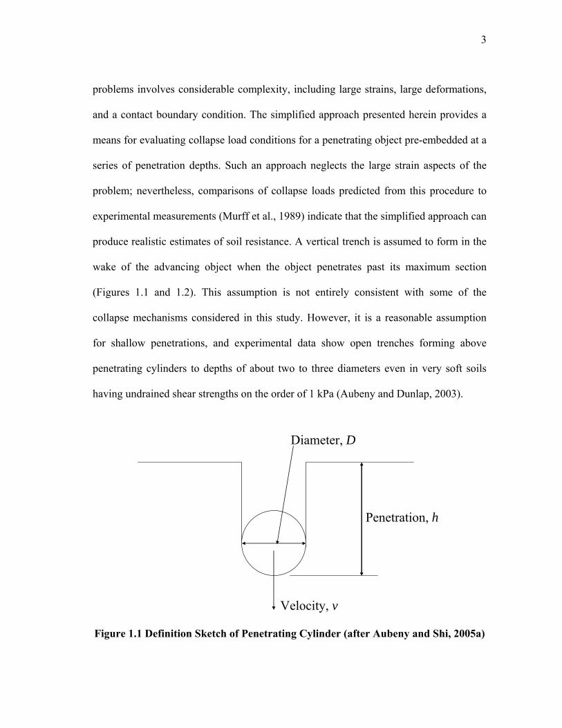
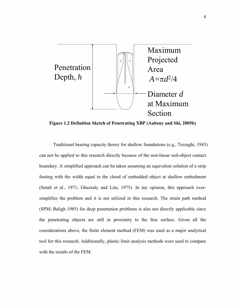
Figures 1.1 and 1.2 illustrate the two penetrating objects considered in this

research. The cylinder is assumed to be infinitely long, i.e., plane strain conditions are

considered, and the XBP is axisymmetric in geometry. Moreover, the cylinder is

assumed to be horizontal and the XBP is vertical. When the penetrating object contacts

the seafloor it will begin to decelerate in a manner controlled by the net effect of its own

weight, the buoyant resistance of the soil, and the shearing resistance of the soil.

Pertinent aspects of the problems include: (1) a soil bearing resistance factor that

increases with penetration depth, (2) disturbance of the soil due to the large penetration

strains, (3) soil shearing resistance that depends on strain rate and therefore penetration

velocity, and (4) variable conditions of penetration velocity. A rigorous analysis of these

3

problems involves considerable complexity, including large strains, large deformations,

and a contact boundary condition. The simplified approach presented herein provides a

means for evaluating collapse load conditions for a penetrating object pre-embedded at a

series of penetration depths. Such an approach neglects the large strain aspects of the

problem; nevertheless, comparisons of collapse loads predicted from this procedure to

experimental measurements (Murff et al., 1989) indicate that the simplified approach can

produce realistic estimates of soil resistance. A vertical trench is assumed to form in the

wake of the advancing object when the object penetrates past its maximum section

(Figures 1.1 and 1.2). This assumption is not entirely consistent with some of the

collapse mechanisms considered in this study. However, it is a reasonable assumption

for shallow penetrations, and experimental data show open trenches forming above

penetrating cylinders to depths of about two to three diameters even in very soft soils

having undrained shear strengths on the order of 1 kPa (Aubeny and Dunlap, 2003).

Penetration, h

Diameter, D

Velocity, v

Figure 1.1 Definition Sketch of Penetrating Cylinder (after Aubeny and Shi, 2005a)

4

PenetrationDepth, h

MaximumProjectedAreaA=πd2/4

Diameter dat MaximumSection

Figure 1.2 Definition Sketch of Penetrating XBP (Aubeny and Shi, 2005b)

Traditional bearing capacity theory for shallow foundations (e.g., Terzaghi, 1943)

can not be applied to this research directly because of the non-linear soil-object contact

boundary. A simplified approach can be taken assuming an equivalent solution of a strip

footing with the width equal to the chord of embedded object at shallow embedment

(Small et al., 1971; Ghazzaly and Lim, 1975). In my opinion, this approach over-

simplifies the problem and it is not utilized in this research. The strain path method

(SPM; Baligh 1985) for deep penetration problems is also not directly applicable since

the penetrating objects are still in proximity to the free surface. Given all the

considerations above, the finite element method (FEM) was used as a major analytical

tool for this research. Additionally, plastic limit analysis methods were used to compare

with the results of the FEM.

5

1.2 Objectives

The objectives of this research may be summarized as follows:

1. Calculate collapse loads for undrained penetration of the cylinder and the

XBP in soft soils;

2. Evaluate the strain rate effects on the collapse loads;

3. Develop predictive models for penetration depth of cylinders and strength

characterization from dynamic measurements of the XBP.

1.3 Outline of Research

This research consists of three components: rate-independent studies, rate-

dependent studies and predictive models.

In the first step we calculate collapse loads for a penetrating object at a series of

penetration depths for quasi-static undrained loading conditions, i.e., the strain rate

dependence of soil strength is not considered at this stage. Through this step, the

relationship between collapse loads and penetration depths is established.

The second step starts from the FEM simulations in the previous step, with the

primary refinement being the incorporation of strain rate-dependent shearing resistance

into the collapse load calculations. The rate-dependent solutions are then evaluated with

reference to the rate-independent solutions. Through this step, the relationship between

collapse loads and penetration velocities is established.

The last step develops simplified predictive models. With the soil shearing

resistance force defined by the collapse loads as a function of penetration depth and

6

penetration velocity, accelerations can be determined at any instant of time for a

penetrating object from simple equations of motion for a rigid body projectile. The

penetration depth can then be evaluated through direct integration. On the other hand,

with the measurements of accelerations at any given time, the soil shearing resistance

force can be inferred and the soil shear strength can be obtained through back-

calculation. The predictive models were further calibrated against experimental

measurements.

7

CHAPTER II

BACKGROUND*

2.1 Plasticity Concepts

Plasticity theory is a very important tool in soil mechanics and it has been

applied extensively. A central concept in plasticity theory is the yield condition, which is

a relationship among stress components at which yield starts to occur (Murff, 2002). The

yield condition can be written as

(σ ) 0ijf = (2.1)

where σij is the stress tensor, representing the six independent components of the stress

at a point (i = 1 to 3 and j = 1 to 3).

For undrained condition of purely cohesive soils, possible yield conditions

include the von Mises condition and the Tresca condition. The von Mises condition is

formulated as

02/12 =− kJ (2.2a)

where J2 is the second invariant of the stress deviation tensor, and k is a constant.

Written in terms of principal stresses

2 2 22 1 2 2 3 3 1

1 [(σ σ ) (σ σ ) (σ σ ) ]6

J = − + − + − (2.2b)

where 1σ , 2σ and 3σ are major, intermediate, and minor principal stresses, respectively.

* Part of this chapter is reprinted with permission of ASCE from “Collapse loads for a cylinder embedded in trench in cohesive soil.” by C. P. Aubeny, H. Shi and J. D. Murff, 2005, International Journal of Geomechanics, ASCE, scheduled to be published in the 2005.

8

The Tresca condition is written as

1 3σ σ2

c−= (2.3)

where c is soil undrained shear strength. For plane strain conditions the two yield

functions above have an identical form (Murff, 2002).

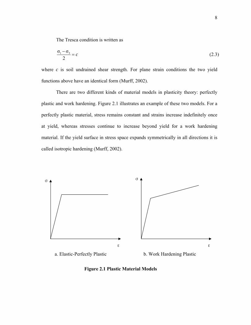
There are two different kinds of material models in plasticity theory: perfectly

plastic and work hardening. Figure 2.1 illustrates an example of these two models. For a

perfectly plastic material, stress remains constant and strains increase indefinitely once

at yield, whereas stresses continue to increase beyond yield for a work hardening

material. If the yield surface in stress space expands symmetrically in all directions it is

called isotropic hardening (Murff, 2002).

σ

ε

σ

ε

a. Elastic-Perfectly Plastic b. Work Hardening Plastic

Figure 2.1 Plastic Material Models

9

The plastic strain increment of a material obeying an associated flow rule is

given as (Drucker and Prager, 1952)

ε λσ

pij

ij

f∂=

∂ (2.4)

where λ = a positive scalar multiplier

f = the plastic potential which is assumed to be the yield function

σij = the corresponding stress

2.2 Plastic Limit Methods

There are two very important plastic limit theorems in estimating collapse loads:

the upper bound theorem and the lower bound theorem. The upper bound theorem states:

“if an estimate of the plastic collapse load of a body is made by equating internal rate of

dissipation of energy to the rate at which external forces do work in any postulated

(kinematically admissible) mechanism of deformation of the body, the estimate will be

either high or correct” (Calladine, 1969). The lower bound theorem states: “if any stress

distribution throughout the structure can be found which is everywhere in equilibrium

internally and balances certain external loads and at the same time does not violate the

yield condition, those loads will be carried safely by the structure” (Calladine, 1969).

This provides a means of estimating the collapse load which is less than or equal to the

true value. If a solution based on both bound theorems yields the same result, then it is

the exact solution.

10

2.2.1 Lower Bound Method

First we will look at the method of characteristic (MOC). For a plane strain

condition we can write the equations of equilibrium as

τσ γxyxxx y

∂∂+ =

∂ ∂ (2.5a)

τ σ

γxy yyx y

∂ ∂+ =

∂ ∂ (2.5b)

where σx , σ y are normal stresses in the x and y direction, τxy is the shear stress on the x

and y planes, γx and γ y are body forces in the x and y directions.

x, xy

y, xy

m 13

2θ

c

-c

Figure 2.2 Mohr’s Circle and Failure Condition (after Murff, 2003)

11

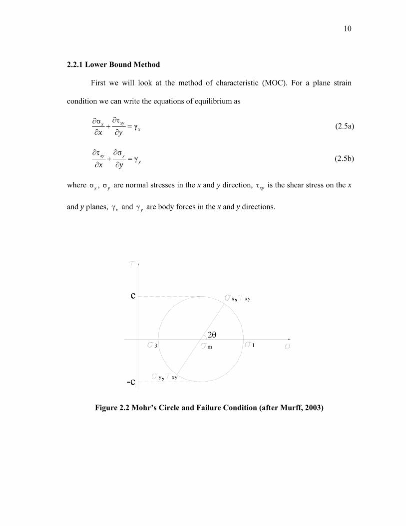
The soil will also satisfy the yield criterion. For an undrained condition we can

write the yield condition as follows, referring to the Mohr’s circle (Figure 2.2)

2 2 2σ σ( ) τ

2x y

xy c−

+ = (2.6)

To simplify the problem we define the mean stress σm as

1σ (σ σ )2m x y= + (2.7)

Furthermore, we define another variable θ which is the angle between major principal

stress 1σ and the x axis.

The following relations can be established from the Mohr’s circle (Figure 2.2)

σ σ cos 2θx m c= + (2.8a)

σ σ cos 2θy m c= − (2.8b)

τ sin 2θxy c= (2.8c)

Substituting the above relations into the equilibrium equations, we get

σ θ θ2 sin 2θ 2 cos 2θ γ cos 2θ sin 2θmx

c cc cx x y x y

∂ ∂ ∂ ∂ ∂− + = − −

∂ ∂ ∂ ∂ ∂ (2.9a)

σ θ θ2 sin 2θ 2 cos 2θ γ cos 2θ sin 2θmy

c cc cy y x y x

∂ ∂ ∂ ∂ ∂+ + = + −

∂ ∂ ∂ ∂ ∂ (2.9b)

It can be shown that (e.g., Sokolovskii, 1965) two sets of equations comprise

characteristics sets of Eqs. 2.9a and 2.9b. These are designated as α and β

characteristics. The corresponding equations are as follows:

On an α characteristic

12

tan(θ )4

dydx

π= − (2.10a)

σ 2 θ (γ ) (γ )m x yc cd cd dx dyy x

∂ ∂− = − + +

∂ ∂ (2.10b)

On a β characteristic

πtan(θ )4

dydx

= + (2.10c)

σ 2 θ (γ ) (γ )m x yc cd cd dx dyy x

∂ ∂+ = + + −

∂ ∂ (2.10d)

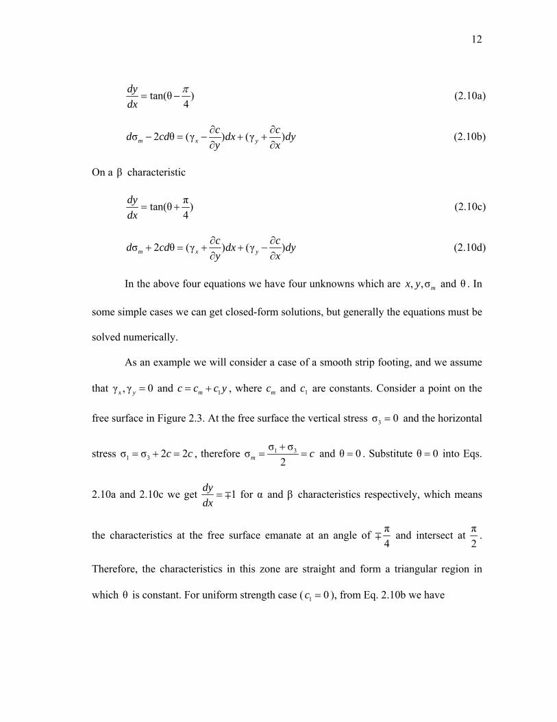
In the above four equations we have four unknowns which are , ,σmx y and θ . In

some simple cases we can get closed-form solutions, but generally the equations must be

solved numerically.

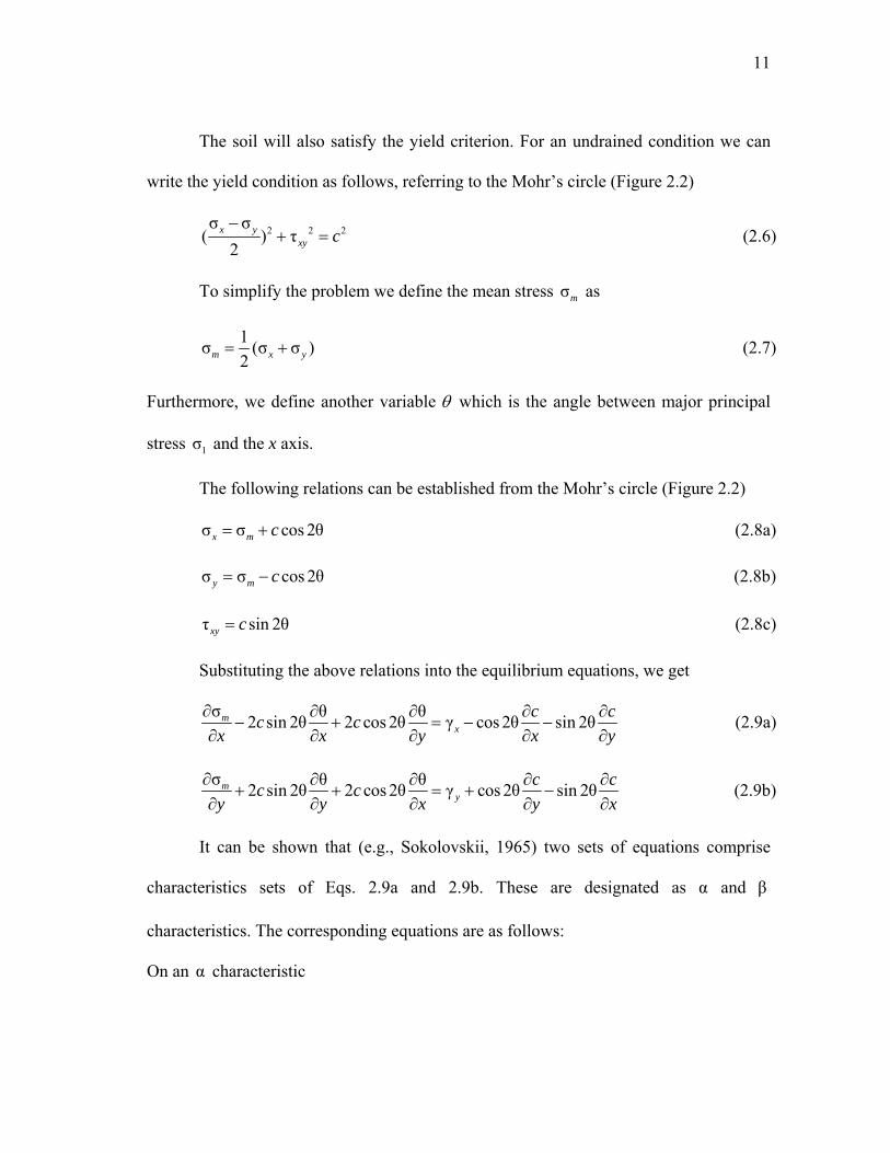
As an example we will consider a case of a smooth strip footing, and we assume

that γ , γ 0x y = and 1mc c c y= + , where mc and 1c are constants. Consider a point on the

free surface in Figure 2.3. At the free surface the vertical stress 3σ 0= and the horizontal

stress 1 3σ σ 2 2c c= + = , therefore 1 3σ σσ2m c+

= = and θ 0= . Substitute θ 0= into Eqs.

2.10a and 2.10c we get 1dydx

= ∓ for α and β characteristics respectively, which means

the characteristics at the free surface emanate at an angle of π4

∓ and intersect at π2

.

Therefore, the characteristics in this zone are straight and form a triangular region in

which θ is constant. For uniform strength case ( 1 0c = ), from Eq. 2.10b we have

13

A B

degenerate 1

3

1

23

4

C

C'C''C'''

C2

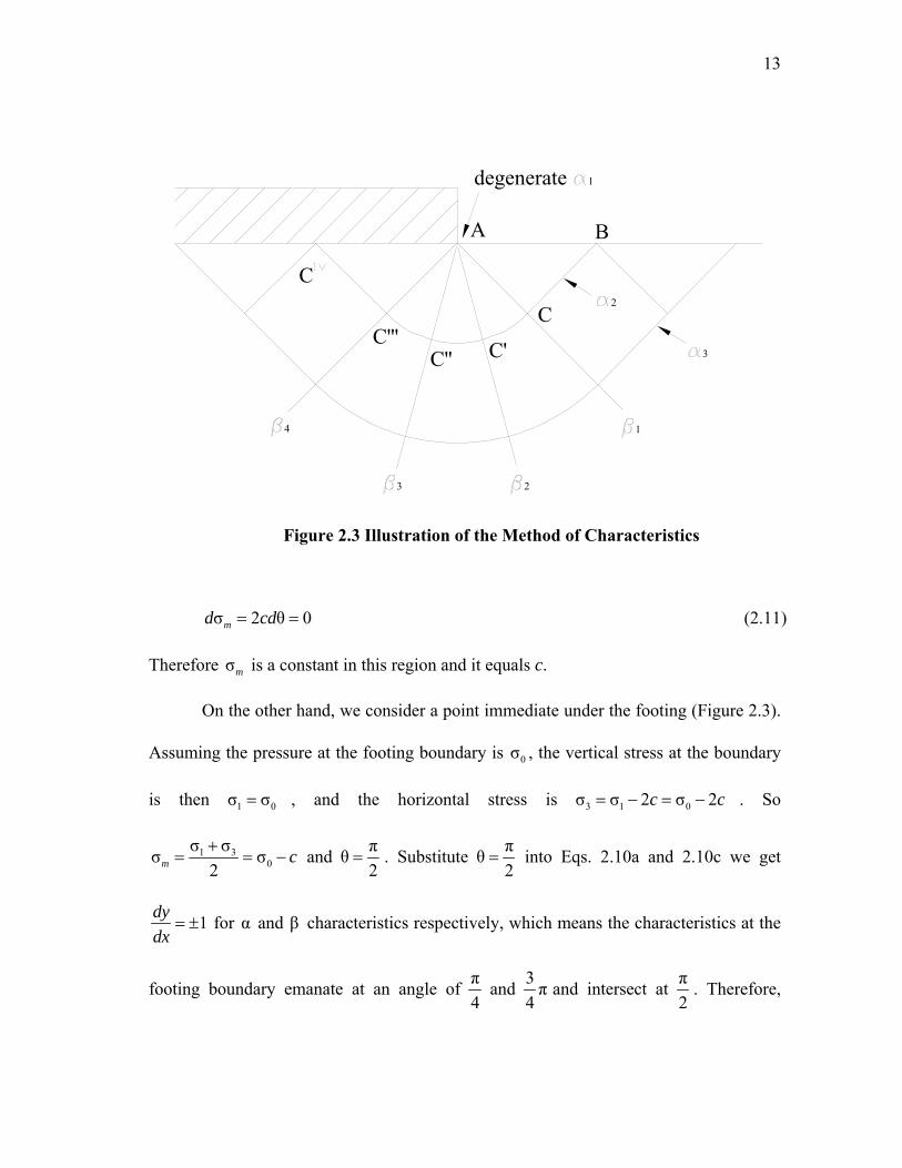
Figure 2.3 Illustration of the Method of Characteristics

σ 2 θ 0md cd= = (2.11)

Therefore σm is a constant in this region and it equals c.

On the other hand, we consider a point immediate under the footing (Figure 2.3).

Assuming the pressure at the footing boundary is 0σ , the vertical stress at the boundary

is then 1 0σ σ= , and the horizontal stress is 3 1 0σ σ 2 σ 2c c= − = − . So

1 30

σ σσ σ2m c+

= = − and πθ2

= . Substitute πθ2

= into Eqs. 2.10a and 2.10c we get

1dydx

= ± for α and β characteristics respectively, which means the characteristics at the

footing boundary emanate at an angle of π4

and 3 π4

and intersect at π2

. Therefore,

14

another triangular region forms under the footing. For uniform strength case σm is

constant in this region and it equals 0σ c− .

The region in between these two triangular regions is generally a shear fan. For

uniform strength case, the β characteristics are straight and the α characteristics are

circular (Murff, 2003). Apparently there is a discontinuity of σm at point A, and the

change in θ through the shear fan is π π ππ4 4 2

− − = (Figure 2.3). From Eq. 2.10b we

have

σ 2 θ πm c c= = (2.12)

Therefore the change in mean stress across the shear fan is πc . Recalling that σm in the

left and the right triangular regions are c and 0σ c− respectively, we have

0σ πc c c− = + (2.13)

0σ (π 2)c= + (2.14)

For the non-uniform strength case ( 1 0c ≠ ), we can solve for the collapse load by

numerical methods. Consider point A and point B at the free surface in Figure 2.3. At

point A and point B the four variables ,σ θ,m x and y are all known, so we can then write

the following difference equations (Murff, 2003):

On an α characteristic

θ θ π( ) tan( )2 4

C BC B C By y x x +

− = − − (2.15a)

1σ σ 2( )(θ θ ) ( )2

C BmC mB C B C B

c c c x x+− − − = − − (2.15b)

15

On a β characteristic

θ θ π( ) tan( )2 4

C AC A C Ay y x x +

− = − + (2.15c)

1σ σ 2( )(θ θ ) ( )2

C AmC mA C A C A

c c c x x+− + − = − − (2.15d)

By combining the above difference equations we can develop recursive relations

as follows:

B A A CA B CBC

CA CB

y y x T x TxT T

− + −=

− (2.16a)

1 [( ) ( ) ( ) ]2C B A C B CB C A CAy y y x x T x x T= + + − + − (2.16b)

1σ σ 2 θ 2 θ (2 )θ2 2

mA mB CB B CA A C A BC

CA CB

c c c x x xc c

− + + + − −=

+ (2.16c)

11σ [σ σ 2 (θ θ ) 2 (θ θ ) ( )]2mC mA mB CB C B CA C A B Ac c c x x= + + − − − + − (2.16d)

where θ θ πtan[( ) ]2 4

A CCAT +

= +

θ θ πtan[( ) ]2 4

B CCBT +

= −

( ) / 2CA C Ac c c= +

( ) / 2CB C Bc c c= +

We can start by assuming θ θC B= on the α characteristic and θ θC A= on the β

characteristic, then we can calculate Cx , ,θC Cy and σmC in turn. Substitute the new

values into the above equations and recycle until the values of , ,θC C Cx y and σmC are

16

within tolerance (e.g., 610− for θC in this study). The change in θ across the shear fan is

π2

. We can divide it into a number of increments, and integrate the mean stress along the

α characteristics.

AA'A''A'''

B

123

CC'C''C'''

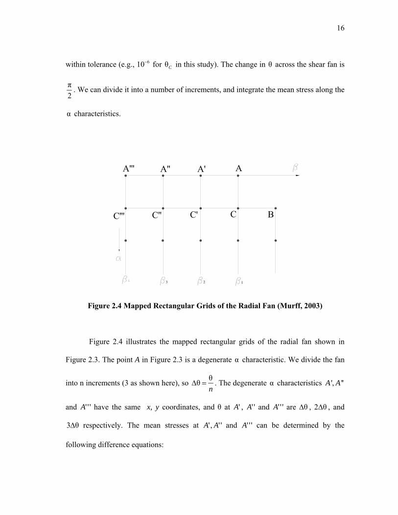
Figure 2.4 Mapped Rectangular Grids of the Radial Fan (Murff, 2003)

Figure 2.4 illustrates the mapped rectangular grids of the radial fan shown in

Figure 2.3. The point A in Figure 2.3 is a degenerate α characteristic. We divide the fan

into n increments (3 as shown here), so θθn

∆ = . The degenerate α characteristics ', ''A A

and '''A have the same x, y coordinates, and θ at 'A , ''A and '''A are θ∆ , 2 θ∆ , and

3 θ∆ respectively. The mean stresses at '',' AA and '''A can be determined by the

following difference equations:

17

σ ( ') σ ( ) 2 θm mA A c= + ∆ (2.17a)

σ ( '') σ ( ') 2 θm mA A c= + ∆ (2.17b)

σ ( ''') σ ( '') 2 θm mA A c= + ∆ (2.17c)

From the conditions at 'A and C we can solve for the conditions ( , ,θ,σmx y ) at 'C using

the previously described recursive method. Then we can solve for the conditions at ''C

and '''C along the α characteristics.

The point IVC under the footing is a boundary on an α characteristic but not on

a β characteristic. We know y and θ at IVC so we can solve the two unknown variables

x and σm by the two α equations:

'''''' '''

'''

θ θ πtan( )2 4

θ θ πtan( )2 4

IV

IV

IV

IV

C CC CC

CCC

y y xx

+− + −

=+

− (2.18a)

''''''

''' 1 '''σ σ 2( )(θ θ ) ( )2

IV

IV IV IVC C

C CmC mC C C

c cc x x

+= + − − − (2.18b)

The vertical stress 0σ at IVC is then

0 0σ σ IVmCc= + (2.19)

For non-uniform strength case the vertical pressure under the footing is not

uniform, therefore we should proceed to the next α characteristic until it reaches the

center of the footing. By integrating the vertical stress and multiplying the result by two

we can obtain the collapse load.

18

To establish a solution of the method of characteristic as a lower bound solution,

the stress field needs to be extended beyond the slip line field into the rigid zone (e.g.

Randolph and Houlsby, 1984). Once this is done the characteristic solution is said to be a

rigorous lower bound (Murff, 2002).

2.2.2 Upper Bound Method

To apply the upper bound method, we define the unknown collapse load F

moving at a velocity 0v , the external work rate is then 0W Fv= . We postulate a

kinematically admissible failure mechanism and velocity field, and then we compute the

internal rate of energy dissipation D satisfying the yield condition and the associated

flow rule. By equating the external work to the internal energy dissipation 0Fv D= , we

can obtain the collapse load F as 0v will cancel out in the equation.

For a material obeying an associated flow rule (Eq. 2.4), the dissipation rate is

calculated by

σ ε λσσ

pij ij ij

ij

fD ∂= =

∂ (2.20)

For undrained plane strain conditions the yield function can be written as

2 1

2 2 2(σ σ ) 1 1[ τ τ ] 0

4 2 2x y

xy yxf c−

= + + − = (2.21)

By substituting Eq. 2.21 into Eq. 2.20 and carrying out the dot product operations we can

obtain

λD c= (2.22)

19

Also, by the associated flow rule the strain rates can be calculated as

λε λ (σ σ )σ 4x x y

x

fc

∂= = −

∂ (2.23a)

λε λ (σ σ )σ 4y x y

y

fc

∂ −= = −

∂ (2.23b)

λε ε λ ττ 2xy yx xy

xy

fc

∂= = =

∂ (2.23c)

We can see that the volumetric strain rate is ε ε ε 0v x y= + = , which implies that the

material is incompressible for this yield condition. By substituting Eqs. 2.23a, 2.23b and

2.23c into the yield condition (Eq. 2.21) we can solve for λ , which is

2 2 2 2 1/ 2λ (2ε 2ε 2ε 2ε )x y xy yx= + + + (2.24)

Therefore

2 2 2 2 1/ 2(2ε 2ε 2ε 2ε )x y xy yxD c= + + + (2.25)

Since ε εx y= − and ε εxy yx= , Eq. 2.25 is reduced to

2 2 1/ 22 (ε ε )x xyD c= + (2.26)

For undrained and general three dimensional conditions, the dissipation functions for

continuously deforming regions are

von Mises condition:

1/ 2(2ε ε )ij ijD c= (2.27)

Tresca condition:

max

max2 ε γ

shearD c c= = (2.28)

20

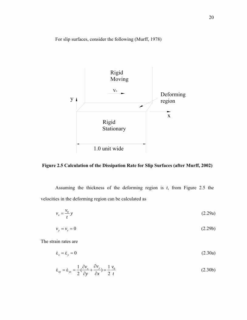
For slip surfaces, consider the following (Murff, 1978)

v0

RigidMoving

RigidStationary

1.0 unit wide

x

yDeforming region

Figure 2.5 Calculation of the Dissipation Rate for Slip Surfaces (after Murff, 2002) Assuming the thickness of the deforming region is t, from Figure 2.5 the

velocities in the deforming region can be calculated as

0x

vv yt

= (2.29a)

0y zv v= = (2.29b)

The strain rates are

ε ε 0x y= = (2.30a)

01 1ε ε ( )2 2

yxxy yx

vv vy x t

∂∂= = + =

∂ ∂ (2.30b)

21

Therefore, the dissipation is

2 1/ 20 012 [( ) ]2

v cvD ct t

= = (2.31)

The total dissipation in the deforming region is then

001TOT

V

cvD DdV t cvt

= = × × =∫ (2.32)

So as 0t → the dissipation on the slip surface is simply

0D cv= (2.33)

where 0v is the relative velocity of slip along the slip surface.

To illustrate the application of the upper bound method we will consider the

same strip footing problem as the lower bound method and a uniform strength condition.

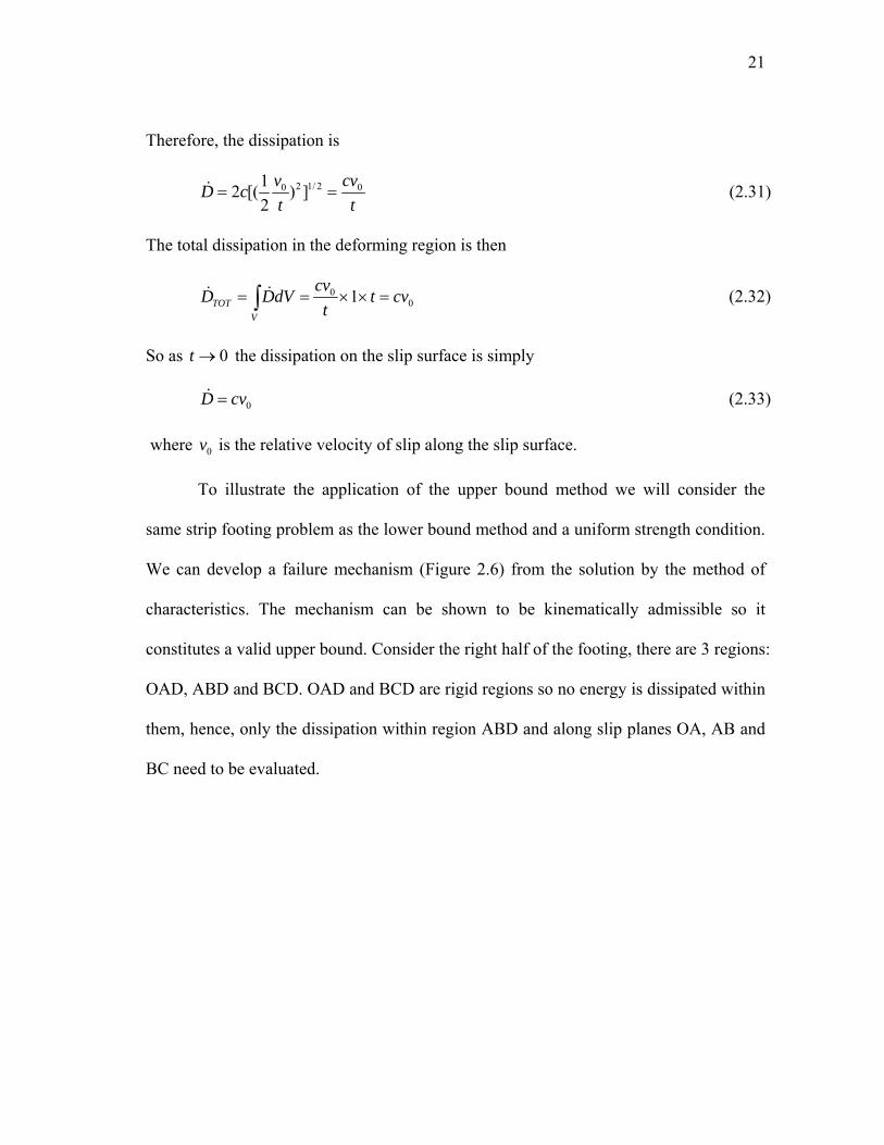
We can develop a failure mechanism (Figure 2.6) from the solution by the method of

characteristics. The mechanism can be shown to be kinematically admissible so it

constitutes a valid upper bound. Consider the right half of the footing, there are 3 regions:

OAD, ABD and BCD. OAD and BCD are rigid regions so no energy is dissipated within

them, hence, only the dissipation within region ABD and along slip planes OA, AB and

BC need to be evaluated.

22

F,v0

o

A B

CD

Figure 2.6 Failure Mechanism Developed from MOC

v0

vH

vR

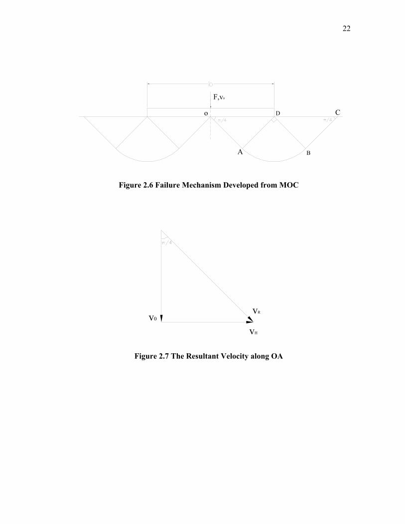
Figure 2.7 The Resultant Velocity along OA

23

From Figure 2.7 we can see that the resultant velocity along OA is

0 0π/ cos 24Rv v v= = . The length of OA is π 2cos

2 4 4b b= , where b is the width of the

footing. Therefore the dissipation along OA is

00

224 2

cv bD c v b= ⋅ ⋅ = (2.34)

The tangential velocity along arc AB is the same as OA, and the length of arc AB is

π 2 2 π2 4 8

b b⋅ = , thus

00

π2π28 4

cv bbD c v= ⋅ ⋅ = (2.35)

The dissipation rate along BC can be evaluated similarly, which is the same as OA.

The tangential velocity within the region ABD is constant, 02tv v= , and the

radial velocity is zero, so the shear strain rate is

02γ ( )t tv v vr r r

∂= − − =

∂ (2.36)

where r is radius of curvature within this region. Thus

π / 2 2 / 4 0 0

0 0

2 πθ4

b v cv bD c rdrdr

= =∫ ∫ (2.37)

where θ is the cylindrical coordinate. Therefore, the total energy dissipation rate is the

sum of the calculated dissipations above and multiply by two, which gives

0 (π 2)TOTD cv b= + (2.38)

Equate the external work rate to the internal dissipation rate, we have

24

0 0 (π 2)Fv cv b= + (2.39)

Thus

/ (π 2)F b c= + (2.40)

which is the same as the lower bound solution. Therefore, it is the exact solution.

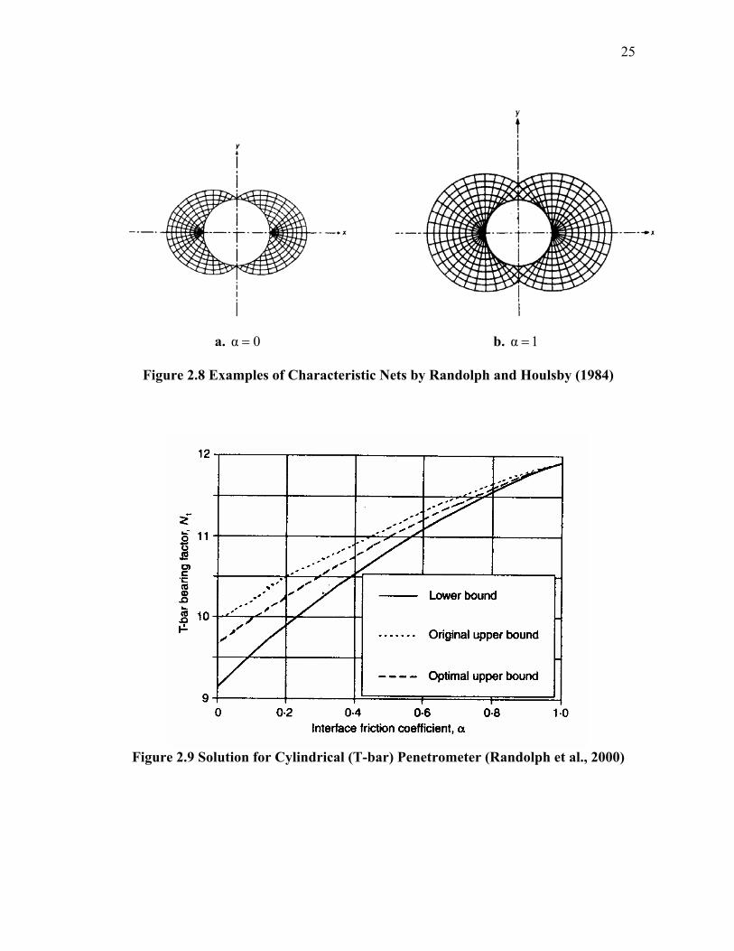
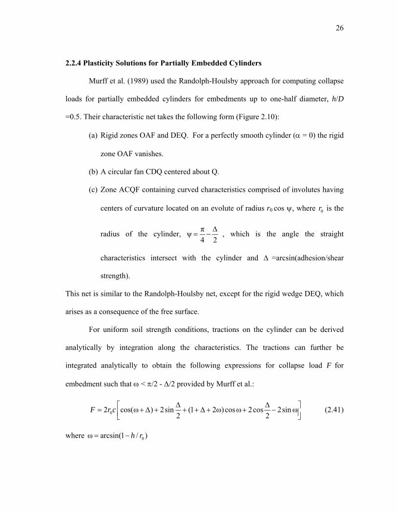
2.2.3 Plasticity Solutions for Fully Embedded Cylinder

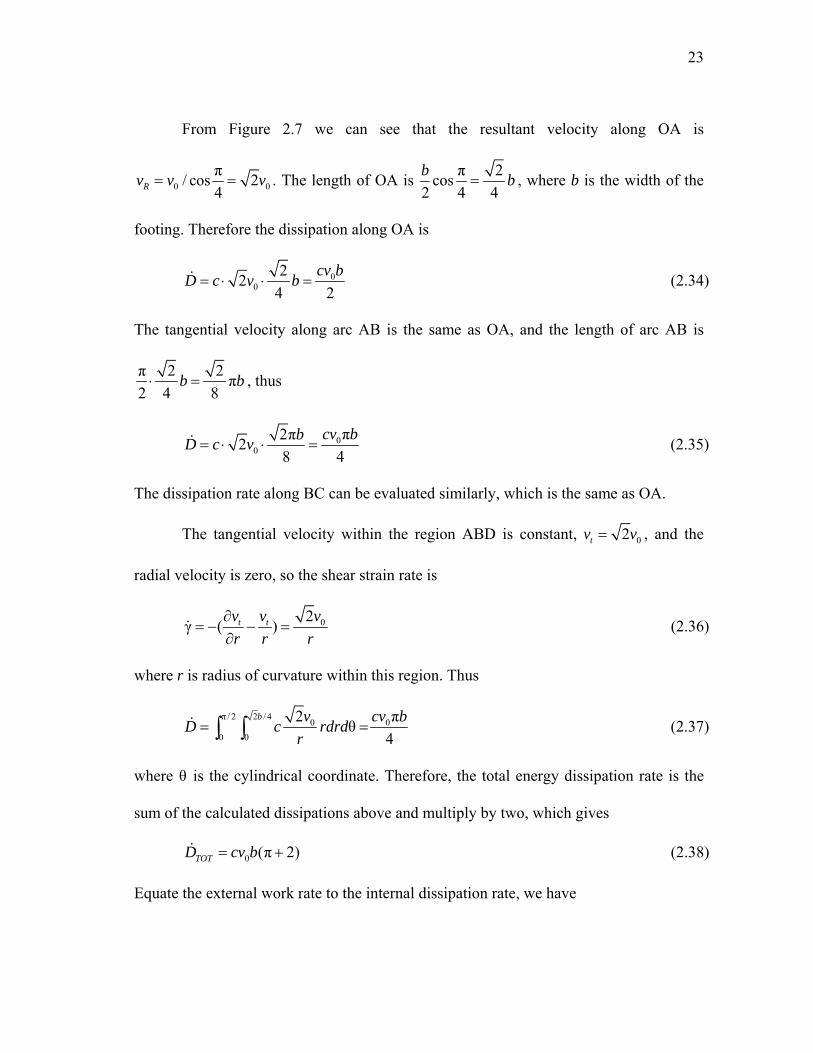
Randolph and Houlsby (1984) applied classical plasticity theory to estimate the

limiting pressure on a fully embedded, laterally translating, circular cylinder unaffected

by any free surface. Their approach employed the method of characteristics (MOC) to

estimate a lower bound limiting resistance, and they used the characteristic net found in

the lower bound solution to derive the velocity field for a collapse mechanism in an

upper bound solution. Figure 2.8 illustrates the characteristic nets for α 0= (smooth pile)

and α 1= (rough pile), where α is the interface adhesion coefficient. For the case of full

adhesion between the soil and cylinder boundary, α=1, their procedure produces

identical lower and upper bound solutions for the normalized collapse load, F/cD =

11.94; i.e., an exact solution. Subsequent study by Murff et al. (1989) indicated some

divergence between lower and upper bound solutions for α<1. The maximum

discrepancy occurs for the case of a perfectly smooth cylinder, where the upper bound

solution exceeds the lower bound (F/cD = 9.14) by about 9%. An optimized upper

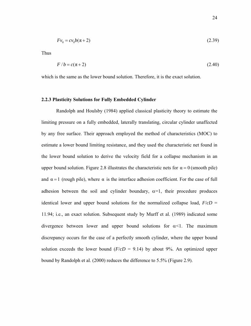
bound by Randolph et al. (2000) reduces the difference to 5.5% (Figure 2.9).

25

a. α 0= b. α 1=

Figure 2.8 Examples of Characteristic Nets by Randolph and Houlsby (1984)

Figure 2.9 Solution for Cylindrical (T-bar) Penetrometer (Randolph et al., 2000)

26

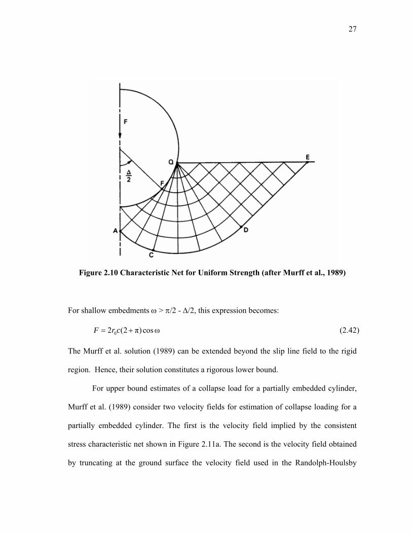
2.2.4 Plasticity Solutions for Partially Embedded Cylinders

Murff et al. (1989) used the Randolph-Houlsby approach for computing collapse

loads for partially embedded cylinders for embedments up to one-half diameter, h/D

=0.5. Their characteristic net takes the following form (Figure 2.10):

(a) Rigid zones OAF and DEQ. For a perfectly smooth cylinder (α = 0) the rigid

zone OAF vanishes.

(b) A circular fan CDQ centered about Q.

(c) Zone ACQF containing curved characteristics comprised of involutes having

centers of curvature located on an evolute of radius r0 cos ψ, where 0r is the

radius of the cylinder, πψ4 2

∆= − , which is the angle the straight

characteristics intersect with the cylinder and ∆ =arcsin(adhesion/shear

strength).

This net is similar to the Randolph-Houlsby net, except for the rigid wedge DEQ, which

arises as a consequence of the free surface.

For uniform soil strength conditions, tractions on the cylinder can be derived

analytically by integration along the characteristics. The tractions can further be

integrated analytically to obtain the following expressions for collapse load F for

embedment such that ω < π/2 - ∆/2 provided by Murff et al.:

02 cos(ω ) 2sin (1 2ω) cosω 2cos 2sinω2 2

F r c ∆ ∆⎡ ⎤= + ∆ + + + ∆ + + −⎢ ⎥⎣ ⎦ (2.41)

where 0ω arcsin(1 / )h r= −

27

Figure 2.10 Characteristic Net for Uniform Strength (after Murff et al., 1989)

For shallow embedments ω > π/2 - ∆/2, this expression becomes:

02 (2 π) cosωF r c= + (2.42)

The Murff et al. solution (1989) can be extended beyond the slip line field to the rigid

region. Hence, their solution constitutes a rigorous lower bound.

For upper bound estimates of a collapse load for a partially embedded cylinder,

Murff et al. (1989) consider two velocity fields for estimation of collapse loading for a

partially embedded cylinder. The first is the velocity field implied by the consistent

stress characteristic net shown in Figure 2.11a. The second is the velocity field obtained

by truncating at the ground surface the velocity field used in the Randolph-Houlsby

28

analysis for a fully embedded cylinder far from a free surface (Figure 2.11b). Both of the

above mechanisms contain velocity jumps across slip planes as well as continuously

deforming regions. Both velocity fields considered above are kinematically admissible

mechanisms; hence, collapse loads derived from them are valid upper bounds.

The energy dissipation rates across the slip planes and deforming regions were

evaluated by Murff et al. (1989). Referring to Figure 2.11a, AFF ' is a rigid zone,

interface AF is inclined at 45 degrees to the vertical direction. The tangential velocity

along AF is 0 / 2tv v= , therefore

0 0 sin( )2

D cv r ∆= (2.43)

Interface ABC is an involute, with the center moving anticlockwise along the evolute,

which is a circle of radius 0 cosψr concentric with the cylinder. The tangential velocity

along ABC is 0 / 2tv v= , so the dissipation rate along the interface is

π / 2 / 2 0

2ωθ

2vD c rd

−∆= ∫ (2.44)

where r is the radius of curvature of ABC, and

0 2π[ 2 sin( ) sinψ ( θ ) cosψ]

2 2 2r r ∆ ∆

= + + − − (2.45)

2θ locates specific straight characteristic.

Interface CD is a circular arc centered at Q. The tangential velocity along CD is

0 / 2tv v= , therefore

π / 4 / 2 ω 0

3π / 4θ

2vD c rd

+∆ += ∫ (2.46)

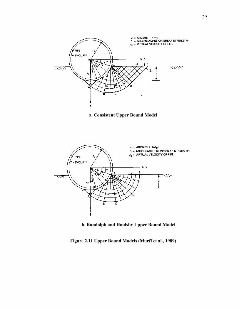
29

a. Consistent Upper Bound Model

b. Randolph and Houlsby Upper Bound Model

Figure 2.11 Upper Bound Models (Murff et al., 1989)

30

where r is the radius of curvature of CD, and

0π[ 2 sin( ) ( ω) cosψ]

2 2 2r r ∆ ∆

= + − − (2.47)

3θ locates specific straight characteristic.

Interface DE is inclined at 45 degrees to the free surface so its length is the same

as QD, which is equal to 0π[ 2 sin( ) ( ω) cosψ]

2 2 2r ∆ ∆

+ − − . The tangential velocity along

CD is 0 / 2tv v= , therefore

0 0π[sin( ) ( ω) cosψ / 2]

2 2 2D v cr ∆ ∆

= + − − (2.48)

Interface FGH is an involute similar to ABC. A tangential velocity discontinuity exists

across FGH equal to

0[cos( / 2)secψ 1/ 2]tv v= ∆ − (2.49)

Thus

π / 2 / 2

2ωθtD c v rd

−∆= ∫ (2.50)

where r is the radius of curvature of FGH, and 0 2π[sinψ ( θ ) cosψ]2 2

r r ∆= + − − .

Interface HI is a circular arc similar to CD. A tangential velocity discontinuity

same as FGH exists across HI, therefore

π / 4 / 2 ω

3π / 4θtD c v rd

+∆ += ∫ (2.51)

where r is the radius of curvature of HI, and 0π( ω) cosψ2 2

r r ∆= − − .

31

Interface IJ is inclined at 45 degrees to the free surface, and its length is the same

as QI, which is equal to 0π( ω) cosψ2 2

r ∆− − . The velocity discontinuity across IJ is

identical to FGH and HI, therefore

0 0cosψ π[cos( ) ]( ω)

2 2 22D v cr ∆ ∆

= − − − (2.52)

For Interface FKQ, the relative velocity between the cylinder and the soil is

0 1 1(cosθ sinθ tanψ)tv v= + (2.53)

The limiting shear stress or adhesion at the soil cylinder interface is sinc ∆ . Thus

π / 2 / 2

0 1ωsin θtD c v r d

−∆= ∆∫ (2.54)

where 1θ locates a specific curved characteristic.

The straight characteristics KGB, QHC and QID all terminate in the rigid region,

therefore no relative velocity develop along them and the energy dissipations are zeros.

Within the deforming region ABCHGF, the tangential velocity is 0 / 2v , and

the radial velocity is zero, so the shear strain rate is

2

0

θ

γ ( )2

t tv v vr r r

∂= − − =

∂ (2.55)

where r is the radius of curvature in each deforming region. Therefore

2

1

π / 2 / 2 02ωθ

2r

r

cvD rdrdr

−∆= ∫ ∫ (2.56)

where the radial integration limits 1r and 2r denote the radius of curvature along FGH

and ABC, respectively.

32

For region CDIH, the tangential velocity and the shear strain rate are in the same

form as within region ABCHGF, thus

2

1

π / 4 / 2 ω 03π / 4θ

2r

r

cvD rdrdr

+∆ += ∫ ∫ (2.57)

where 1r and 2r denote the radii of curvature along HI and CD, respectively.

Region DEJI is a rigid zone, so the dissipation within it is zero. For region

FGHQK, the tangential velocity along the curved characteristics is 0 1sinθ / cosψtv v= ,

and the radius of curvature in the region is 0 1 2[sinψ (θ θ ) cosψ]r r= + − , so the shear

strain rate is

2

0 1 0 12

θ 0

cosθ sinθγ ( ) ( )cos ψ cosψ

t tv v v vr r r r

∂= − − = − −

∂ (2.58)

Thus

1π / 2 / 2 θ

0 2 1ω ωγ cosψ θ θD c rr d d

−∆= ∫ ∫ (2.59)

For region HIQ, the tangential velocity and the shear strain rate are in the same form as

within region FGHQK, i.e., 0 1 0 12

0

cosθ sin θγ ( )cos ψ cosψ

v vr r

= − − , but the radius of curvature is

0 1(θ ω) cosψr r= − . Similarly we have

π / 2 / 2 π / 4 / 2 ω

0 3 1ω π / 4γ cosψ θ θD c rr d d

−∆ +∆ += ∫ ∫ (2.60)

For region IJQ, a new set of axes is taken to facilitate the calculation. Q is the

new origin and y ' runs along QID. The tangential velocity along the straight

characteristics is

33

' 0 1sinθ / cosψxv v= (2.61)

Recalling that 0 1' (θ ω) cosψy r= − , the shear strain rate becomes

'' 0 12

0

cosθγ' ' cos ψ

yx vv vy x r

∂∂= + =

∂ ∂ (2.62)

Thus

π ' 0 12 2

0 12ω 00

cosθ cosψ ' θcos ψ

y vD cr dx dr

∆−

= ∫ ∫ (2.63)

For the Randolph-Houlsby upper bound model, the energy dissipation rates are

the same except slip planes IJ, DE and deforming regions DEJI and IJQ (Figure 2.11b).

Slip plane DE is a circular arc extended from CD, thus

π / 4 0

30θ

2vD c rd= ∫ (2.64)

Slip plane is also a circular arc extended from HI, thus

π / 4

30θtD c v rd= ∫ (2.65)

The deforming region DEJI is an extension of region CDIH, thus

2

1

π / 4 030θ

2r

r

cvD rdrdr

= ∫ ∫ (2.66)

Region IJQ is an extension of the circular shear fan HIQ, thus

π / 2 / 2 π / 4

0 3 1ω 0γ cosψ θ θD c rr d d

−∆= ∫ ∫ (2.67)

By evaluating the integrals and summing all the energy dissipation rates for slip

planes and deforming regions together, we obtain the total internal dissipation TOTD . The

external work rate is

34

0v TOTW F v D= = (2.68)

From the equation above we can obtain vF and the collapse load by multiplying vF by 2

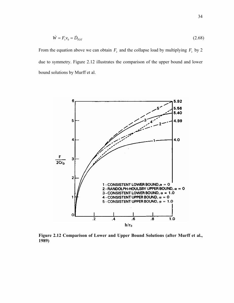
due to symmetry. Figure 2.12 illustrates the comparison of the upper bound and lower

bound solutions by Murff et al.

h/r0

Figure 2.12 Comparison of Lower and Upper Bound Solutions (after Murff et al., 1989)

35

2.3 Finite Element Method

In essence, the finite element method (FEM) is an approximate method

implemented by discretizing the solution domain into a number of “finite elements”. By

doing so we can choose interpolation functions and construct approximate equations for

each element. We can solve for the unknown variables by assembling all the element

equations together and imposing the boundary conditions (Reddy, 1993).

2.3.1 FEM Theory

There are two main reasons to discretize the domain (Reddy, 1993). The first

reason is to approximate the geometry, e.g., we can approximate a curve by a set of

straight lines. The accuracy of the approximation will depend on the refinement of the

mesh. If one keeps increasing the refinement of a mesh, the solution will tend to

converge on the exact value. The second reason is to approximate the solution over each

element instead of the whole domain, which is more difficult to do.

As an example we will consider a solid mechanics frame work (Aubeny, 2003).

The basic solution variable is the displacement vector [ ]u , and the strain-displacement

relationship is

[ε] [ ][ ]B u= (2.69)

where [B] is the strain-displacement operator. The stress-strain relationship can be

established as

[σ] [ ][ε]C= (2.70)

36

where [C] is the constitutive matrix. The governing differential equation in tensor form

is

σ 0f∇ + =i (2.71)

which can also be written as

[ ] [σ] [ ]TB f= (2.72)

where [ ]f is the externally applied force vector. Combine Eqs. 2.69, 2.70 and 2.72, we

obtain the following:

[ ] [ ][ ][ ] [ ] 0TB C B u f− = (2.73)

or

[ ][ ] [ ]K u f= (2.74)

where [K] is the stiffness matrix and [ ] [ ] [ ][ ]TK B C B= .

In each element, we approximate the displacement by interpolation functions as

follows:

ˆ[ ] [ ][ ]u H u= (2.75)

where [H] is the interpolation matrix, and ˆ[ ]u is the nodal displacement vector. If we

multiply the left hand side of Eq. (2.73) by a weighting function matrix [ ] [ ]Tw H= we

obtain the following:

ˆ[ ] [ ][ ][ ] [ ] [ ] [ ]T TB C B u H f R− = (2.76)

where [R] is the residual error term. By the method of weighed residuals (MWR) we

integrate it over the element and let it equal zero, which can be written as

37

ˆ[ ] [ ][ ][ ] [ ] [ ] 0T T

V V

B C B u dV H f dV− =∫ ∫ (2.77)

For each element the element stiffness matrix [ ] [ ] [ ][ ]Te

V

K B C B dV= ∫ , and the force

vector [ ] [ ] [ ]Te

V

F H f dV= ∫ . Therefore the element equation in matrix form is

[ ] [ ] [ ]e eK u F= (2.78)

The element equations can be assembled together based on the satisfaction of

inter-element continuity and equilibrium. The global stiffness matrix and force vector

can be written as

#

1[ ] [ ]

elements

G ei

K K=

= ∑ (2.79)

#

1[ ] [ ]

elements

G ei

F F=

= ∑ (2.80)

To solve the assembly equations, the boundary conditions need to be applied for the

specific problem, such as a prescribed displacement, an applied load etc. The equations

can be solved by mathematical operations. If necessary, the solutions can be post-

processed into graphical or tabular presentation.

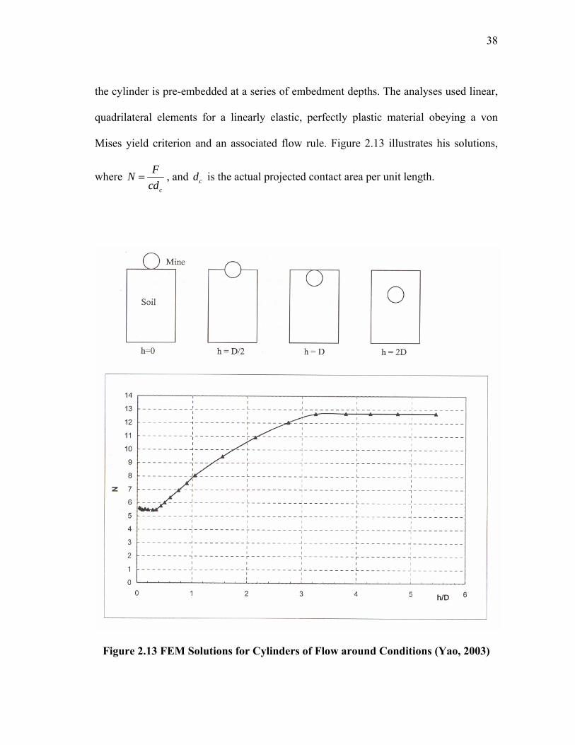
2.3.2 FEM Studies for Cylinders of Flow-around Conditions

Finite element studies on undrained penetration of rough cylindrical mines in

uniform soils were carried forward at Texas A&M University by Yao (2003), with the

assumption that the soil will flow around the cylinder after the penetration depth exceeds

one half diameter (Figure 2.13). He calculated the quasi-static collapse loads assuming

38

the cylinder is pre-embedded at a series of embedment depths. The analyses used linear,

quadrilateral elements for a linearly elastic, perfectly plastic material obeying a von

Mises yield criterion and an associated flow rule. Figure 2.13 illustrates his solutions,

where c

FNcd

= , and cd is the actual projected contact area per unit length.

Figure 2.13 FEM Solutions for Cylinders of Flow around Conditions (Yao, 2003)

39

2.4 Rate Dependent Properties of Soil

The dependence of undrained shear strength of soil on applied rate of strain has

long been recognized (Casagrande and Wilson, 1951). Rate dependency of soil on

undrained shear strength has been studied extensively both in triaxial compression tests

(e.g., Bjerrum et al., 1958; Richardson and Whitman; 1963; Richardson, 1963; Ladd et

al., 1972; Alberro and Santoyo, 1973; Berre and Bjerrum, 1973; Vaid and Campanella,

1977; Hight, 1983; Lefebvre and LeBoeuf, 1987; Sheahan et al., 1996) and in vane shear

tests (e.g., Skempton, 1948; Cadling & Odenstad, 1950; Aas, 1965; Halwachs, 1972;

Wiesel, 1973; Torstensson, 1977; Smith & Richards, 1975; Perlow & Richards, 1977;

Schapery & Dunlap, 1978; Sharifounnasab & Ulrich, 1985; Roy & LeBlanc, 1988;

Biscontin and Pestana, 2001). The relationship between undrained shear strength and

strain rate in triaxial tests is often expressed by a logarithmic relationship (Sheahan et al.,

1996), while either a logarithmic or a power law can be formulated in terms of rotation

rates in vane shear tests (Biscontin and Pestana, 2001). The Biscontin-Pestana data also

suggest that substituting peripheral velocity for rotation rate provides a better basis for

interpreting test data from different vane blade radius dimensions.

A possible predictive framework for strain rate dependence is that of a viscous

fluid model (e.g., Whitney and Rodin, 2001). Viscous models have been used very

effectively in practical applications such as pipeline embedment in soft seafloor soils

(Schapery and Dunlap, 1984). This framework has the advantage that the material

parameters describing strain rate effects can be estimated from variable strain rate shear

tests in a relatively straight-forward manner. A chief disadvantage is that soil shearing

40

resistance decays to negligible levels as penetration velocity approaches zero, which can

lead to unrealistic results, depending on the problem.

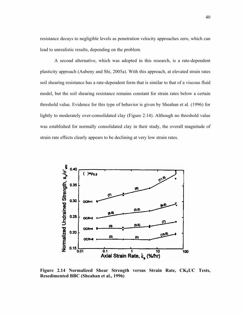
A second alternative, which was adopted in this research, is a rate-dependent

plasticity approach (Aubeny and Shi, 2005a). With this approach, at elevated strain rates

soil shearing resistance has a rate-dependent form that is similar to that of a viscous fluid

model, but the soil shearing resistance remains constant for strain rates below a certain

threshold value. Evidence for this type of behavior is given by Sheahan et al. (1996) for

lightly to moderately over-consolidated clay (Figure 2.14). Although no threshold value

was established for normally consolidated clay in their study, the overall magnitude of

strain rate effects clearly appears to be declining at very low strain rates.

Figure 2.14 Normalized Shear Strength versus Strain Rate, CK0UC Tests, Resedimented BBC (Sheahan et al., 1996)

41

An appealing feature of the rate-dependent plasticity approach is that the

framework follows naturally from well-established methods for estimating collapse

loads from rate-independent plasticity theory. Hence, rate-independent solutions can

provide a useful frame of reference from which strain rate effects can be evaluated. A

drawback of the approach is that the threshold strain rate is at present ill-defined, and the

magnitude of the threshold may in fact be so low that the assumption of undrained

shearing no longer becomes valid.

2.5 Experimental Studies

The experimental studies relevant to this research include the mini-vane shear

tests, the penetration tests and the XBP tests. The details of these tests and their

interpretations are discussed in the following section.

2.5.1 Miniature Vane Shear Tests

The miniature vane (MV) shear test consists of inserting a four-bladed vane into

a soil sample and rotating it at a constant rate to determine the maximum torque to be

developed (ASTM, 2001). For isotropic materials, the torque can be converted to

undrained shear strength by the following equation (Murff, 1980):

2 34/(2 / cos ν)3

k T R L Rπ π= + (2.81)

where k = undrained shear strength

T = torque

R = radius of the blade

42

L = height of the vane

ν = angle of vane taper

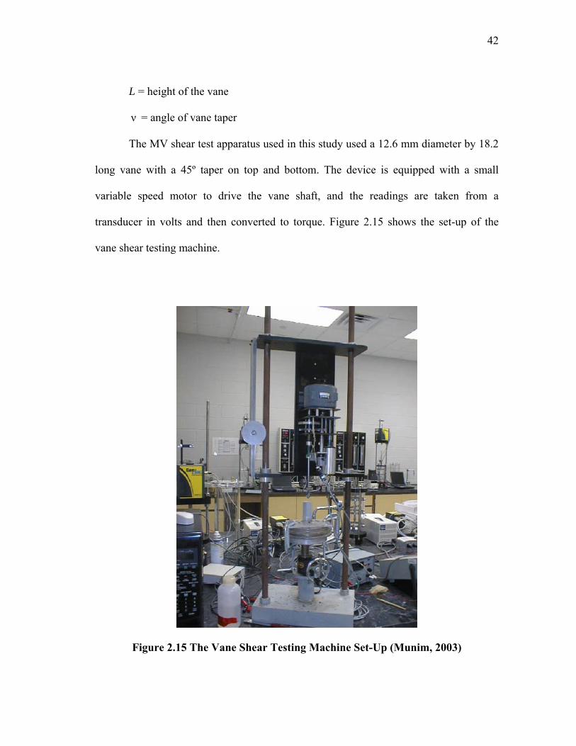
The MV shear test apparatus used in this study used a 12.6 mm diameter by 18.2

long vane with a 45º taper on top and bottom. The device is equipped with a small

variable speed motor to drive the vane shaft, and the readings are taken from a

transducer in volts and then converted to torque. Figure 2.15 shows the set-up of the

vane shear testing machine.

Figure 2.15 The Vane Shear Testing Machine Set-Up (Munim, 2003)

43

2.5.2 Penetration Tests

The penetration tests (Aubeny and Dunlap, 2003) involve penetration

measurements of a model cylinder for various conditions of cylinder weight and mudline

velocity. The soils used in the tests were reconstituted marine clays collected from the

Gulf of Mexico seafloor approximately 32 km south of Port Aransas, Texas. The soils

were collected using a box core sampler and transported in 0.21-m3 (55-gal) drums to the

laboratory. The natural soils were processed to remove shells, mixed to achieve a

uniform mixture, and dried from a water content of about 69% down to 52%. The

reconstituted soil had a liquid limit of 44-45 and a plastic limit of 20-22. Given that the

water content of the soils was well above the liquid limit, sampling and laboratory

strength testing was not practical. Soil strength in the test basin was therefore estimated

using a hand-held vane shear apparatus rotated at a rate of 0.02 rad/sec. Typical

strengths were on the order of 1-1.5kPa. This test method can not be considered highly

accurate, but given the limited options for measuring the strength of shallow, extremely

soft soils, the above methods were adopted for characterizing soil strength.

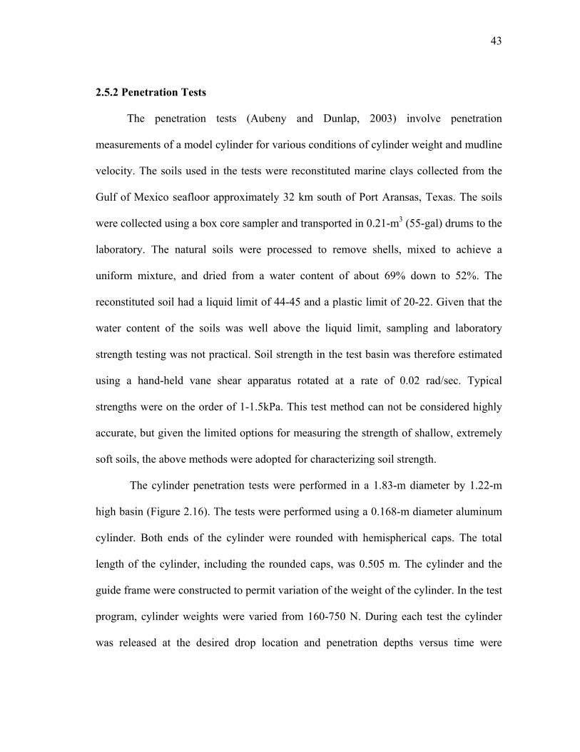
The cylinder penetration tests were performed in a 1.83-m diameter by 1.22-m

high basin (Figure 2.16). The tests were performed using a 0.168-m diameter aluminum

cylinder. Both ends of the cylinder were rounded with hemispherical caps. The total

length of the cylinder, including the rounded caps, was 0.505 m. The cylinder and the

guide frame were constructed to permit variation of the weight of the cylinder. In the test

program, cylinder weights were varied from 160-750 N. During each test the cylinder

was released at the desired drop location and penetration depths versus time were

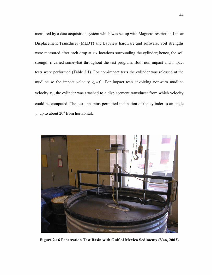
44

measured by a data acquisition system which was set up with Magneto-restriction Linear

Displacement Transducer (MLDT) and Labview hardware and software. Soil strengths

were measured after each drop at six locations surrounding the cylinder; hence, the soil

strength c varied somewhat throughout the test program. Both non-impact and impact

tests were performed (Table 2.1). For non-impact tests the cylinder was released at the

mudline so the impact velocity 0 0v = . For impact tests involving non-zero mudline

velocity 0v , the cylinder was attached to a displacement transducer from which velocity

could be computed. The test apparatus permitted inclination of the cylinder to an angle

β up to about 20o from horizontal.

Figure 2.16 Penetration Test Basin with Gulf of Mexico Sediments (Yao, 2003)

45

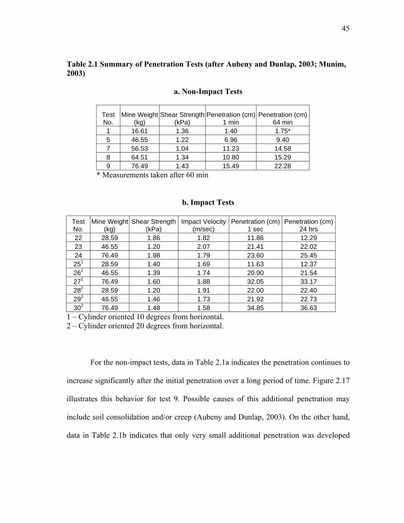
Table 2.1 Summary of Penetration Tests (after Aubeny and Dunlap, 2003; Munim, 2003)

a. Non-Impact Tests

Test No.

Mine Weight (kg)

Shear Strength (kPa)

Penetration (cm) 1 min

Penetration (cm) 64 min

1 16.61 1.36 1.40 1.75* 5 46.55 1.22 6.96 9.40 7 56.53 1.04 11.23 14.58 8 64.51 1.34 10.80 15.29 9 76.49 1.43 15.49 22.28

* Measurements taken after 60 min

b. Impact Tests

Test No.

Mine Weight (kg)

Shear Strength (kPa)

Impact Velocity (m/sec)

Penetration (cm) 1 sec

Penetration (cm) 24 hrs

22 28.59 1.86 1.82 11.86 12.29 23 46.55 1.20 2.07 21.41 22.02 24 76.49 1.98 1.79 23.60 25.45 251 28.59 1.40 1.69 11.63 12.37 261 46.55 1.39 1.74 20.90 21.54 271 76.49 1.60 1.88 32.05 33.17 282 28.59 1.20 1.91 22.00 22.40 292 46.55 1.46 1.73 21.92 22.73 302 76.49 1.48 1.58 34.85 36.63

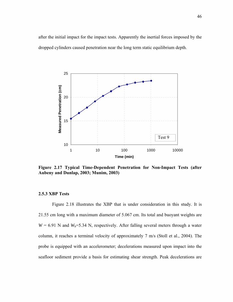
1 – Cylinder oriented 10 degrees from horizontal. 2 – Cylinder oriented 20 degrees from horizontal. For the non-impact tests, data in Table 2.1a indicates the penetration continues to

increase significantly after the initial penetration over a long period of time. Figure 2.17

illustrates this behavior for test 9. Possible causes of this additional penetration may

include soil consolidation and/or creep (Aubeny and Dunlap, 2003). On the other hand,

data in Table 2.1b indicates that only very small additional penetration was developed

46

after the initial impact for the impact tests. Apparently the inertial forces imposed by the

dropped cylinders caused penetration near the long term static equilibrium depth.

10

15

20

25

1 10 100 1000 10000

Time (min)

Mea

sure

d Pe

netr

atio

n (c

m)

Figure 2.17 Typical Time-Dependent Penetration for Non-Impact Tests (after Aubeny and Dunlap, 2003; Munim, 2003)

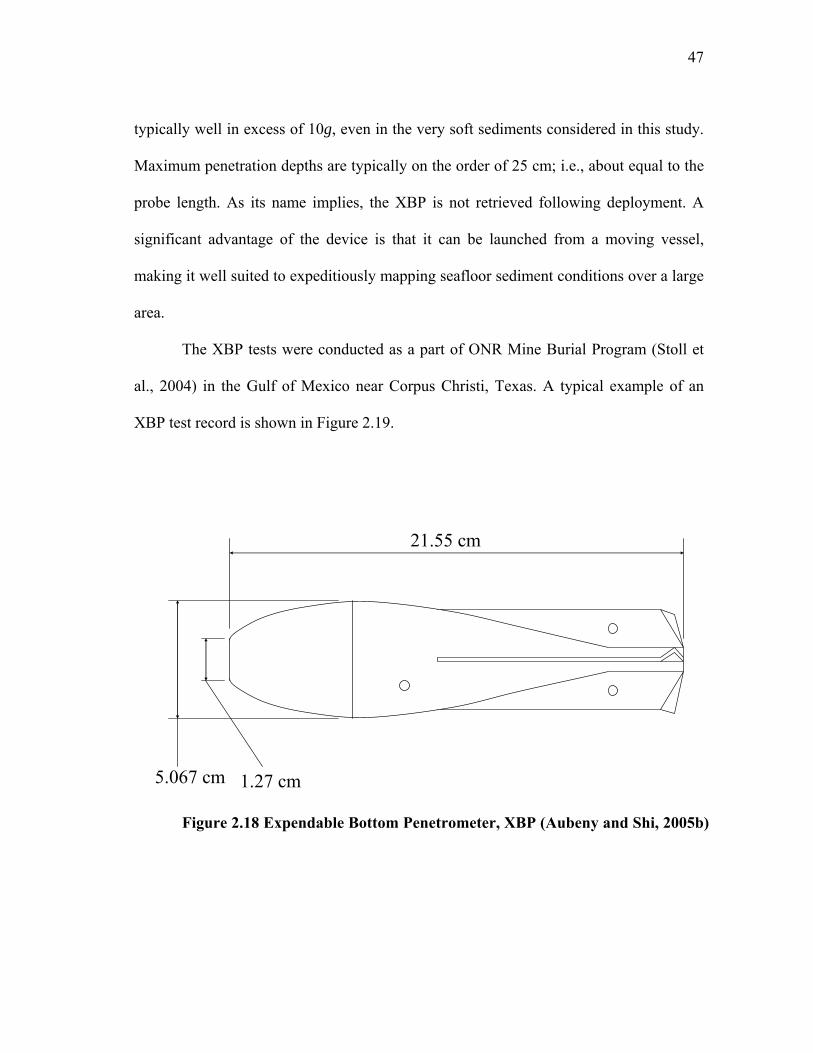
2.5.3 XBP Tests

Figure 2.18 illustrates the XBP that is under consideration in this study. It is

21.55 cm long with a maximum diameter of 5.067 cm. Its total and buoyant weights are

W = 6.91 N and Wb=5.34 N, respectively. After falling several meters through a water

column, it reaches a terminal velocity of approximately 7 m/s (Stoll et al., 2004). The

probe is equipped with an accelerometer; decelerations measured upon impact into the

seafloor sediment provide a basis for estimating shear strength. Peak decelerations are

Test 9

47

typically well in excess of 10g, even in the very soft sediments considered in this study.

Maximum penetration depths are typically on the order of 25 cm; i.e., about equal to the

probe length. As its name implies, the XBP is not retrieved following deployment. A

significant advantage of the device is that it can be launched from a moving vessel,

making it well suited to expeditiously mapping seafloor sediment conditions over a large

area.

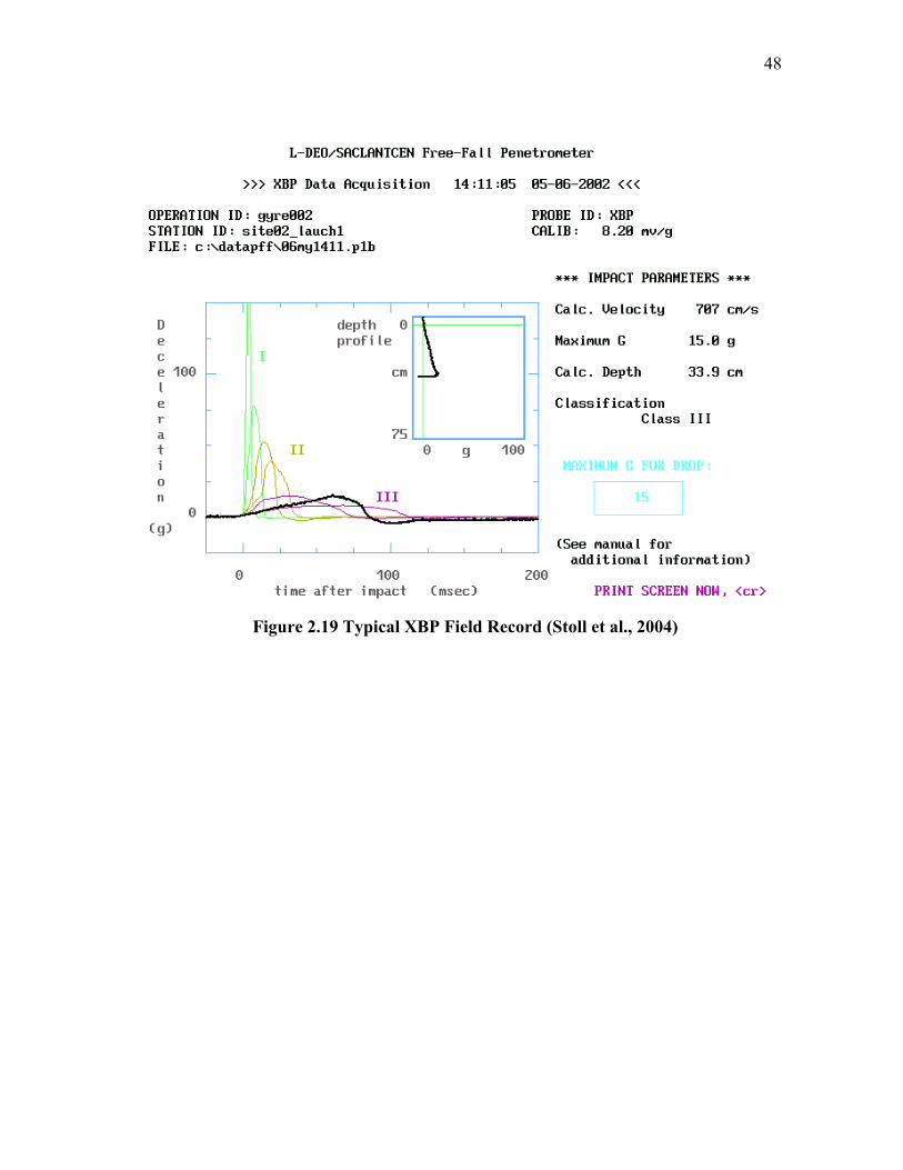
The XBP tests were conducted as a part of ONR Mine Burial Program (Stoll et

al., 2004) in the Gulf of Mexico near Corpus Christi, Texas. A typical example of an

XBP test record is shown in Figure 2.19.

5.067 cm 1.27 cm

21.55 cm

Figure 2.18 Expendable Bottom Penetrometer, XBP (Aubeny and Shi, 2005b)

48

Figure 2.19 Typical XBP Field Record (Stoll et al., 2004)

49

CHAPTER III

RATE-INDEPENDENT STUDIES*

3.1 Plastic Limit Analysis

Plastic limit analyses were carried forward for collapse loads of horizontal

cylinders embedded in open trenches. The analysis extends the study by Murff et al.

(1989) to both non-uniform strength conditions and embedments exceeding one-half

diameter. Following the precedent of previous studies (e.g., Davis and Booker, 1973) the

analysis considers linearly varying strength profiles where the undrained shear strength c

at a depth z can be characterized by the following expression:

1mc c c z= + (3.1)

where mc is the strength at the ground surface (mudline) and 1c is the rate of strength

increase with depth. Such strength variation is conveniently characterized in terms of a

dimensionless parameter η:

1η / mc D c= (3.2)

3.1.1 Lower Bound Analysis

MOC collapse load calculations for smooth cylinders and non-uniform strength

conditions were calculated by the method illustrated in Chapter II, with the differences

here being the change in θ across the shear fan and the boundary condition at the soil-

* Part of this chapter is reprinted with permission of ASCE from “Collapse loads for a cylinder embedded in trench in cohesive soil.” by C. P. Aubeny, H. Shi and J. D. Murff, 2005, International Journal of Geomechanics, ASCE, scheduled to be published in the 2005.

50

cylinder interface. The angle across the singularity is π π ππ-( -ω)- - =ω2 4 4

, where ω is

defined in Figure 2.11. For the boundary point IVC which is immediately under the

cylinder in this case (Figure 3.1), the major principal stress 1σ is the normal stress at the

cylinder boundary. Therefore, from Figure 3.1 we have

2 20 0( )IV IVC C

x r y r h= − + − (3.3)

01θ tan ( )IV

IV

IV

CC

C

y r hx

− + −= (3.4)

Also, from the α -characteristic equation we have

'''

''' '''

θ θ π( ) tan( )2 4

IV

IV IVC C

C C C Cy y x x

+= + − − (3.5)

By combining Eqs. 3.3, 3.4 and 3.5, we obtain the following equation:

'''

''' '''

01

2 20 02 2

0 0

tan [ ] θ( ) π[ ( ) ] tan

2 4

IV

IV

IV IV

CC

CC C C C

y r h

r y r hy y r y r h x

− + −⎧ ⎫+⎪ ⎪

− + −⎪ ⎪= + − + − − −⎨ ⎬⎪ ⎪⎪ ⎪⎩ ⎭

(3.6)

By solving this equation we can obtain IVCy , then we can calculate IVC

x and θ IVC by Eqs.

3.3 and 3.4, and we can calculate σ IVmC by the following α -characteristic equation:

'''

''' ''' '''1σ σ 2( )(θ θ ) ( )2

IV

IV IV IVC C

mC mC C C C C

c cc x x

+= + − − − (3.7)

The normal stress at the interface is then

σ σ IV IVmC Cc= + (3.8)

51

r0

h

x

y

CIV

y +r0-hCIV

xCIV

θ

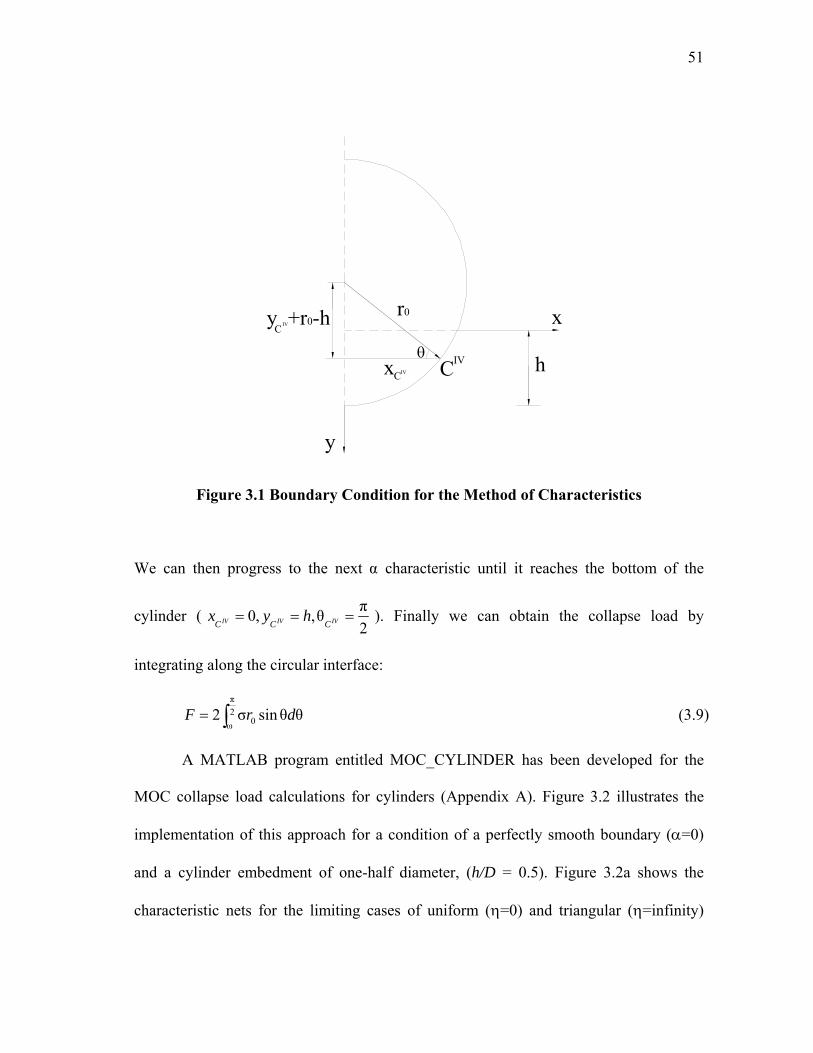
Figure 3.1 Boundary Condition for the Method of Characteristics

We can then progress to the next α characteristic until it reaches the bottom of the

cylinder ( π0, ,θ2IV IV IVC C C

x y h= = = ). Finally we can obtain the collapse load by

integrating along the circular interface:

π2

0ω2 σ sinθ θF r d= ∫ (3.9)

A MATLAB program entitled MOC_CYLINDER has been developed for the

MOC collapse load calculations for cylinders (Appendix A). Figure 3.2 illustrates the

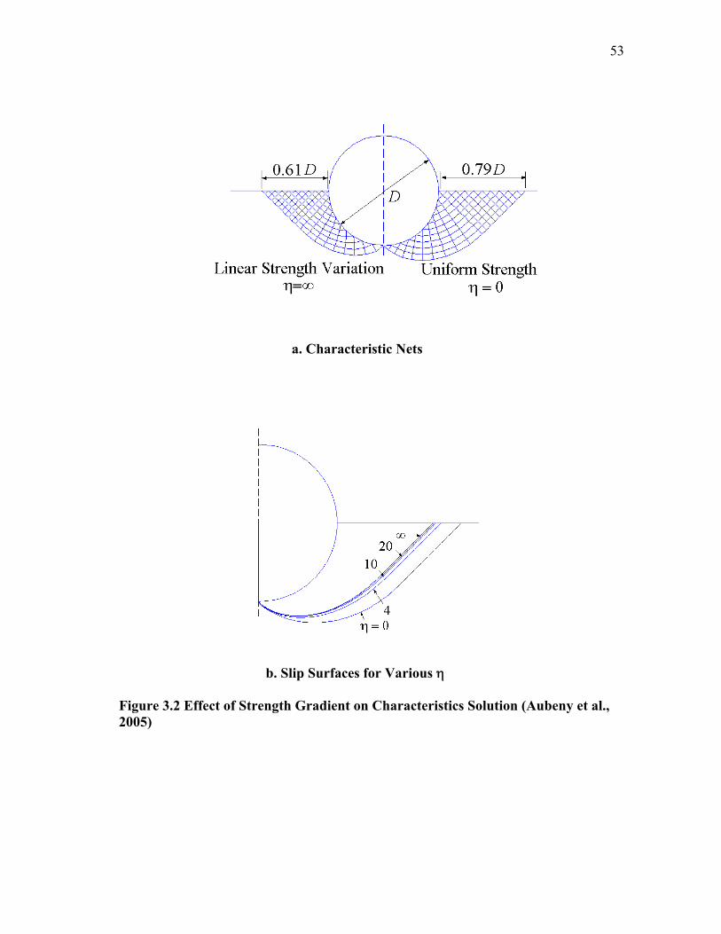
implementation of this approach for a condition of a perfectly smooth boundary (α=0)

and a cylinder embedment of one-half diameter, (h/D = 0.5). Figure 3.2a shows the

characteristic nets for the limiting cases of uniform (η=0) and triangular (η=infinity)

52

strength profiles. With the introduction of a strength gradient, the size of the slip line

field noticeably diminishes; that is, the failure zone is more localized. For example, at

the free surface the lateral extent of the slip line field for η = infinity is nearly 25 percent

less than that for η = 0, 0.61D versus 0.79D. Slip line field boundaries for intermediate

strength profiles are shown in Figure 3.2b. These again depict a continuous trend of

decreasing depth and lateral extent as η increases. For the uniform strength case (η = 0),

the stress field can be extended into the rigid region hence the MOC solution constitutes

a valid lower bound (Murff et al., 1989). However, this task has not been undertaken in

the present study for the non-homogeneous case; hence, some caution should be

exercised in interpreting these solutions as the lower bounds.

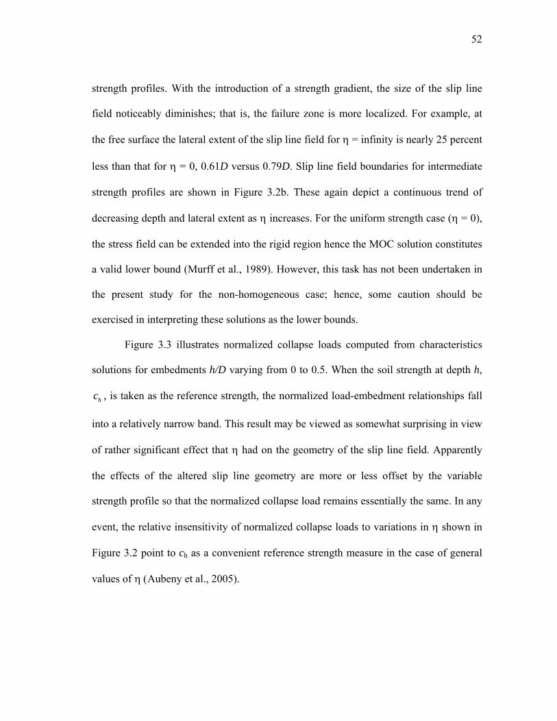
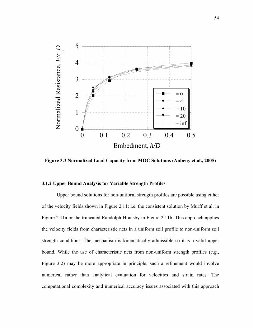
Figure 3.3 illustrates normalized collapse loads computed from characteristics

solutions for embedments h/D varying from 0 to 0.5. When the soil strength at depth h,

hc , is taken as the reference strength, the normalized load-embedment relationships fall

into a relatively narrow band. This result may be viewed as somewhat surprising in view

of rather significant effect that η had on the geometry of the slip line field. Apparently

the effects of the altered slip line geometry are more or less offset by the variable

strength profile so that the normalized collapse load remains essentially the same. In any

event, the relative insensitivity of normalized collapse loads to variations in η shown in

Figure 3.2 point to ch as a convenient reference strength measure in the case of general

values of η (Aubeny et al., 2005).

53

a. Characteristic Nets

b. Slip Surfaces for Various η

Figure 3.2 Effect of Strength Gradient on Characteristics Solution (Aubeny et al., 2005)

54

0

1

2

3

4

5

0 0.1 0.2 0.3 0.4 0.5

= 0= 4= 10= 20 = infN

orm

aliz

ed R

esis

tanc

e, F

/chD

Embedment, h/D

Figure 3.3 Normalized Load Capacity from MOC Solutions (Aubeny et al., 2005)

3.1.2 Upper Bound Analysis for Variable Strength Profiles

Upper bound solutions for non-uniform strength profiles are possible using either

of the velocity fields shown in Figure 2.11; i.e. the consistent solution by Murff et al. in

Figure 2.11a or the truncated Randolph-Houlsby in Figure 2.11b. This approach applies

the velocity fields from characteristic nets in a uniform soil profile to non-uniform soil

strength conditions. The mechanism is kinematically admissible so it is a valid upper

bound. While the use of characteristic nets from non-uniform strength profiles (e.g.,

Figure 3.2) may be more appropriate in principle, such a refinement would involve

numerical rather than analytical evaluation for velocities and strain rates. The

computational complexity and numerical accuracy issues associated with this approach

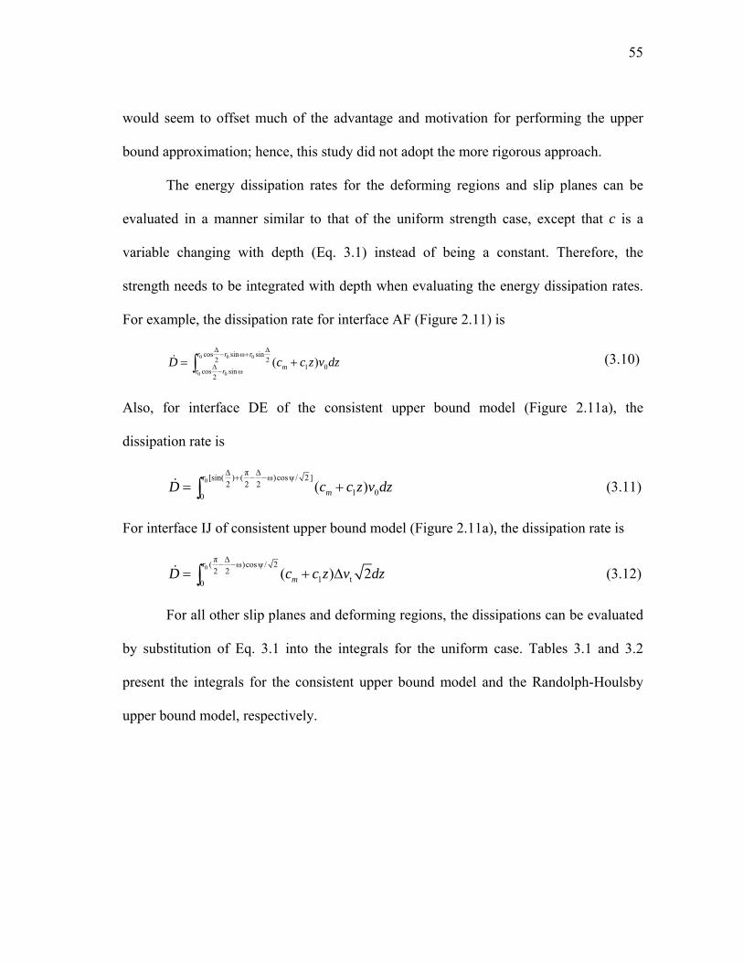
55

would seem to offset much of the advantage and motivation for performing the upper

bound approximation; hence, this study did not adopt the more rigorous approach.

The energy dissipation rates for the deforming regions and slip planes can be

evaluated in a manner similar to that of the uniform strength case, except that c is a

variable changing with depth (Eq. 3.1) instead of being a constant. Therefore, the

strength needs to be integrated with depth when evaluating the energy dissipation rates.

For example, the dissipation rate for interface AF (Figure 2.11) is

0 0 0

0 0

cos sinω sin2 2

1 0cos sinω2

( )r r r

mr rD c c z v dz

∆ ∆− +

∆−

= +∫ (3.10)

Also, for interface DE of the consistent upper bound model (Figure 2.11a), the

dissipation rate is

0π[sin( ) ( ω)cosψ / 2 ]

2 2 21 00

( )r

mD c c z v dz∆ ∆

+ − −= +∫ (3.11)

For interface IJ of consistent upper bound model (Figure 2.11a), the dissipation rate is

0π( ω)cosψ / 22 2

1 t0( ) 2

r

mD c c z v dz∆

− −= + ∆∫ (3.12)

For all other slip planes and deforming regions, the dissipations can be evaluated

by substitution of Eq. 3.1 into the integrals for the uniform case. Tables 3.1 and 3.2

present the integrals for the consistent upper bound model and the Randolph-Houlsby

upper bound model, respectively.

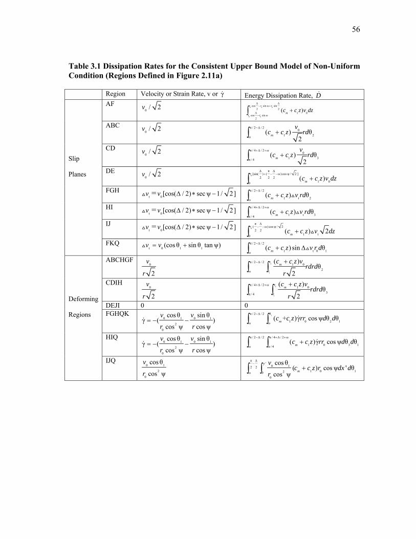
56

Table 3.1 Dissipation Rates for the Consistent Upper Bound Model of Non-Uniform Condition (Regions Defined in Figure 2.11a) Region Velocity or Strain Rate, v or γ Energy Dissipation Rate, D

AF 0 / 2v 0 0 0

0 0

cos sin ω sin2 2

1 0cos sin ω

2

( )r r r

mr r

c c z v dz∆ ∆

− +

∆−

+∫

ABC 0 / 2v π / 2 / 2

01 2ω

( ) θ2

m

vc c z rd

−∆

+∫

CD 0 / 2v π / 4 / 2 ω

01 3π / 4

( ) θ2

m

vc c z rd

+∆ +

+∫

DE 0 / 2v 0

π[sin( ) ( ω ) cosψ / 2 ]

2 2 21 00

( )r

mc c z v dz∆ ∆

+ − −

+∫ FGH

tv = 0[cos( / 2) secψ 1/ 2]v ∆ ∗ − π / 2 / 2

1 t 2ω( ) θmc c z v rd

−∆

+∫ HI

tv = 0[cos( / 2) secψ 1/ 2]v ∆ ∗ − π / 4 / 2 ω

1 t 3π / 4( ) θmc c z v rd

+∆ +

+∫ IJ

tv = 0[cos( / 2) secψ 1/ 2]v ∆ ∗ − 0

π( ω ) cosψ / 2

2 21 t0

( ) 2r

mc c z v dz∆

− −

+∫

Slip Planes

FKQ t 0 1 1(cos θ sin θ tan ψ)v v= + π / 2 / 2

1 t 0 1ω( ) sin θmc c z v r d

−∆

+ ∆∫ ABCHGF

0

2

v

r 2

1

π / 2 / 21 0

2ω

( )θ

2

rm

r

c c z vrdrd

r

−∆ +∫ ∫

CDIH 0

2

v

r 2

1

π / 4 / 2 ω1 0

3π / 4

( )θ

2

rm

r

c c z vrdrd

r

+∆ + +∫ ∫

DEJI 0 0 FGHQK

0 1 0 1

2

0

cosθ sin θγ ( )

cos ψ cosψ

v v

r r= − −

1π / 2 / 2 θ

1 0 2 1ω ω( + )γ cosψ θ θmc c z rr d d

−∆

∫ ∫

HIQ 0 1 0 1

2

0

cosθ sin θγ ( )

cos ψ cosψ

v v

r r= − −

π / 2 / 2 π / 4 / 2 ω

1 0 3 1ω π / 4( )γ cosψ θ θmc c z rr d d

−∆ +∆ +

+∫ ∫

Deforming Regions

IJQ 0 1

2

0

cosθ

cos ψ

v

r

π'

0 12 21 0 12ω 0

0

cos θ( ) cosψ ' θ

cos ψ

y

m

vc c z r dx d

r

∆−

+∫ ∫

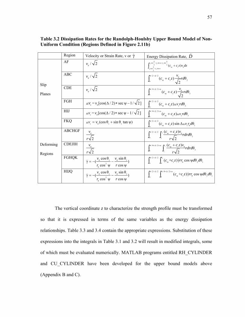
57

Table 3.2 Dissipation Rates for the Randolph-Houlsby Upper Bound Model of Non-Uniform Condition (Regions Defined in Figure 2.11b) Region Velocity or Strain Rate, v or γ Energy Dissipation Rate, D

AF 0 / 2v 0 0 0

0 0

cos sin ω sin2 2

1 0cos sin ω

2

( )r r r

mr r

c c z v dz∆ ∆

− +

∆−

+∫

ABC 0 / 2v π / 2 / 2

01 2ω

( ) θ2

m

vc c z rd

−∆

+∫

CDE 0 / 2v π / 4 / 2 ω

01 30

( ) θ2

m

vc c z rd

+∆ +

+∫

FGH tv = 0[cos( / 2) secψ 1/ 2]v ∆ ∗ − π / 2 / 2

1 t 2ω( ) θmc c z v rd

−∆

+∫

HIJ tv = 0[cos( / 2) secψ 1/ 2]v ∆ ∗ − π / 4 / 2 ω

1 t 30( ) θmc c z v rd

+∆ +

+∫

Slip Planes

FKQ t 0 1 1(cos θ sin θ tan ψ)v v= + π / 2 / 2

1 t 0 1ω( ) sin θmc c z v r d

−∆

+ ∆∫

ABCHGF 0

2

v

r 2

1

π / 2 / 21 0

2ω

( )θ

2

rm

r

c c z vrdrd

r

−∆ +∫ ∫

CDEJIH 0

2

v

r 2

1

π / 4 / 2 ω1 0

30

( )θ

2

rm

r

c c z vrdrd

r

+∆ + +∫ ∫

FGHQK 0 1 0 1

2

0

cos θ sin θγ ( )

cos ψ cosψ

v v

r r= − −

1π / 2 / 2 θ

1 0 2 1ω ω( + )γ cosψ θ θmc c z rr d d

−∆

∫ ∫

Deforming Regions

HIJQ 0 1 0 1

2

0

cos θ sin θγ ( )

cos ψ cosψ

v v

r r= − −

π / 2 / 2 π / 4 / 2 ω

1 0 3 1ω 0( + )γ cosψ θ θmc c z rr d d

−∆ +∆ +

∫ ∫

The vertical coordinate z to characterize the strength profile must be transformed

so that it is expressed in terms of the same variables as the energy dissipation

relationships. Table 3.3 and 3.4 contain the appropriate expressions. Substitution of these

expressions into the integrals in Table 3.1 and 3.2 will result in modified integrals, some

of which must be evaluated numerically. MATLAB programs entitled RH_CYLINDER

and CU_CYLINDER have been developed for the upper bound models above

(Appendix B and C).

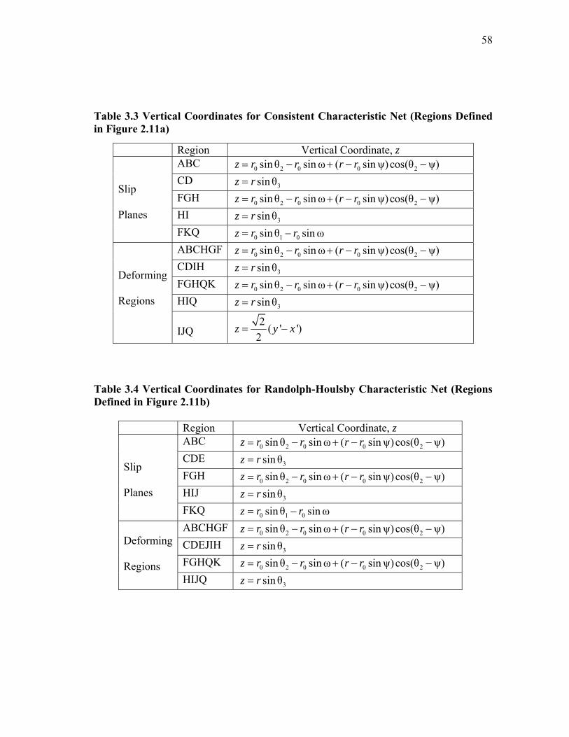
58

Table 3.3 Vertical Coordinates for Consistent Characteristic Net (Regions Defined in Figure 2.11a)

Table 3.4 Vertical Coordinates for Randolph-Houlsby Characteristic Net (Regions Defined in Figure 2.11b)

Region Vertical Coordinate, z ABC 0 2 0 0 2sinθ sinω ( sinψ) cos(θ ψ)z r r r r= − + − − CDE 3sinθz r= FGH 0 2 0 0 2sinθ sinω ( sinψ) cos(θ ψ)z r r r r= − + − −

HIJ 3sinθz r=

Slip Planes

FKQ 0 1 0sinθ sinωz r r= −

ABCHGF 0 2 0 0 2sinθ sinω ( sinψ) cos(θ ψ)z r r r r= − + − −

CDEJIH 3sinθz r=

FGHQK 0 2 0 0 2sinθ sinω ( sinψ) cos(θ ψ)z r r r r= − + − −

Deforming Regions

HIJQ 3sinθz r=

Region Vertical Coordinate, z ABC 0 2 0 0 2sinθ sinω ( sinψ) cos(θ ψ)z r r r r= − + − −

CD 3sinθz r=

FGH 0 2 0 0 2sinθ sinω ( sinψ) cos(θ ψ)z r r r r= − + − −

HI 3sinθz r=

Slip Planes

FKQ 0 1 0sinθ sinωz r r= −

ABCHGF 0 2 0 0 2sinθ sinω ( sinψ) cos(θ ψ)z r r r r= − + − −

CDIH 3sinθz r= FGHQK 0 2 0 0 2sinθ sinω ( sinψ) cos(θ ψ)z r r r r= − + − − HIQ 3sinθz r=

Deforming Regions

IJQ

2 ( ' ')2

z y x= −

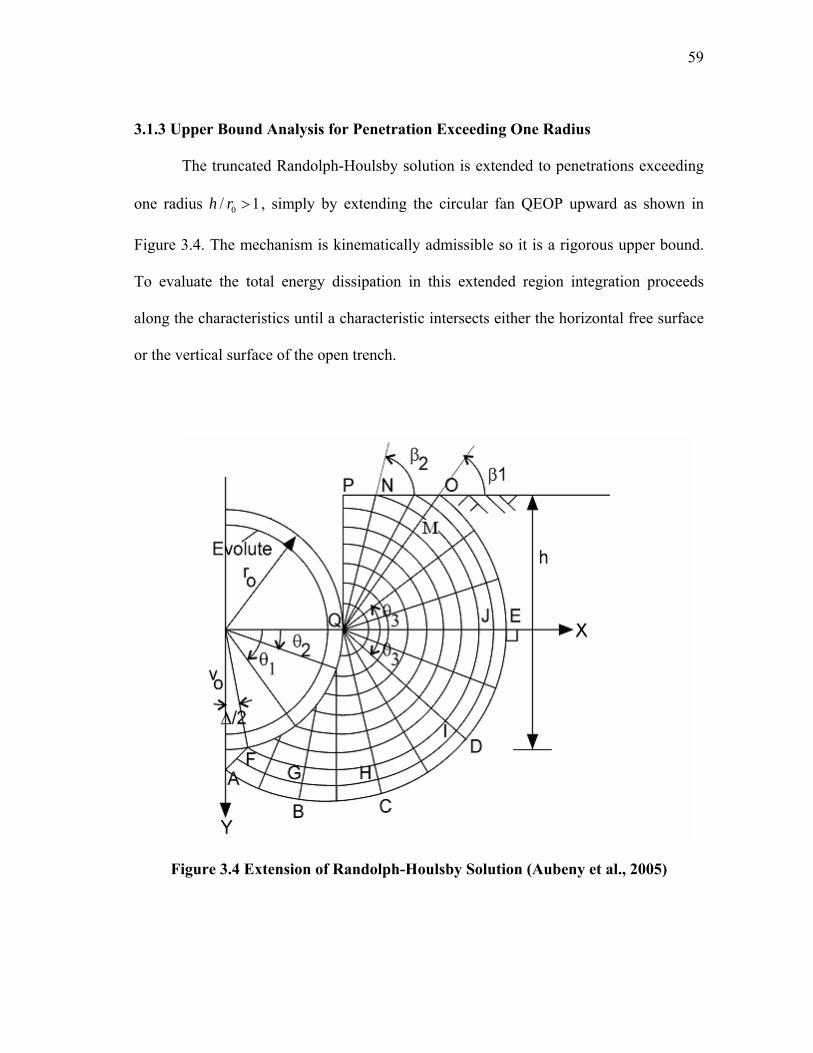
59

3.1.3 Upper Bound Analysis for Penetration Exceeding One Radius

The truncated Randolph-Houlsby solution is extended to penetrations exceeding

one radius 0/ 1h r > , simply by extending the circular fan QEOP upward as shown in

Figure 3.4. The mechanism is kinematically admissible so it is a rigorous upper bound.

To evaluate the total energy dissipation in this extended region integration proceeds

along the characteristics until a characteristic intersects either the horizontal free surface

or the vertical surface of the open trench.

Figure 3.4 Extension of Randolph-Houlsby Solution (Aubeny et al., 2005)

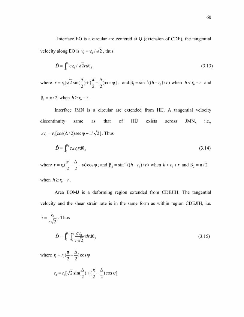
60

Interface EO is a circular arc centered at Q (extension of CDE), the tangential

velocity along EO is 0 / 2tv v= , thus

1β

0 30/ 2 θD cv rd= ∫ (3.13)

where 0π[ 2 sin( ) ( )cosψ]

2 2 2r r ∆ ∆

= + − , and 11 0β sin (( ) / )h r r−= − when 0h r r< + and

1β π / 2= when 0h r r≥ + .

Interface JMN is a circular arc extended from HIJ. A tangential velocity

discontinuity same as that of HIJ exists across JMN, i.e.,

0[cos( / 2)secψ 1/ 2]tv v= ∆ − . Thus

2β

30θtD c v rd= ∫ (3.14)

where 0 ( ω) cosψ2 2

r r π ∆= − − , and 1

2 0β sin (( ) / )h r r−= − when 0h r r< + and 2β π / 2=

when 0h r r≥ + .

Area EOMJ is a deforming region extended from CDEJIH. The tangential

velocity and the shear strain rate is in the same form as within region CDEJIH, i.e.

0γ2

vr

= . Thus

1 2

1

β 030θ

2r

r

cvD rdrdr

= ∫ ∫ (3.15)

where 1 0π( ) cosψ2 2

r r ∆= −

2 0π[ 2 sin( ) ( ) cosψ]

2 2 2r r ∆ ∆

= + −

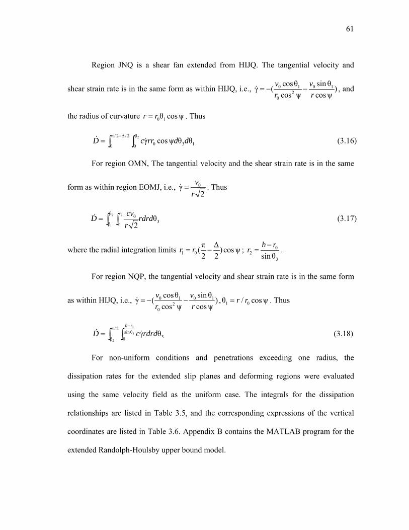
61

Region JNQ is a shear fan extended from HIJQ. The tangential velocity and

shear strain rate is in the same form as within HIJQ, i.e., 0 1 0 12

0

cosθ sin θγ ( )cos ψ cosψ

v vr r

= − − , and

the radius of curvature 0 1θ cosψr r= . Thus

2π / 2 / 2 β

0 3 10 0γ cosψ θ θD c rr d d

−∆= ∫ ∫ (3.16)

For region OMN, The tangential velocity and the shear strain rate is in the same

form as within region EOMJ, i.e., 0γ2

vr

= . Thus

2 2

1 1

β 03βθ

2r

r

cvD rdrdr

= ∫ ∫ (3.17)

where the radial integration limits 1 0π ∆( ) cosψ2 2

r r= − ; 02

3sinθh rr −

= .

For region NQP, the tangential velocity and shear strain rate is in the same form

as within HIJQ, i.e., 0 1 0 12

0

cosθ sinθγ ( )cos ψ cosψ

v vr r

= − − , 1 0θ / cosψr r= . Thus

0

3

2

π / 2sinθ

3β 0γ θ

h r

D c rdrd−

= ∫ ∫ (3.18)

For non-uniform conditions and penetrations exceeding one radius, the

dissipation rates for the extended slip planes and deforming regions were evaluated

using the same velocity field as the uniform case. The integrals for the dissipation

relationships are listed in Table 3.5, and the corresponding expressions of the vertical

coordinates are listed in Table 3.6. Appendix B contains the MATLAB program for the

extended Randolph-Houlsby upper bound model.

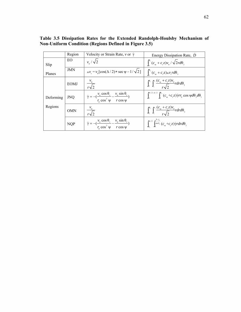
62

Table 3.5 Dissipation Rates for the Extended Randolph-Houlsby Mechanism of Non-Uniform Condition (Regions Defined in Figure 3.5)

Region Velocity or Strain Rate, v or γ Energy Dissipation Rate, D EO

0 / 2v 1β

1 0 30( ) / 2 θmc c z v rd+∫

Slip Planes

JMN tv = 0[cos( / 2) secψ 1/ 2]v ∆ ∗ − 2β

1 t 30( ) θmc c z v rd+∫

EOMJ 0

2

v

r 1 2

1

β1 0

30

( )θ

2

rm

r

c c z vrdrd

r

+∫ ∫

JNQ 0 1 0 1

2

0

cos θ sin θγ ( )

cos ψ cosψ

v v

r r= − −

2π / 2 / 2 β

1 0 3 10 0( + )γ cosψ θ θmc c z rr d d

−∆

∫ ∫

OMN 0

2

v

r 2 2

1 1

β1 0

3β

( )θ

2

rm

r

c c z vrdrd

r

+∫ ∫

Deforming Regions

NQP 0 1 0 1

2

0

cos θ sin θγ ( )

cos ψ cosψ

v v

r r= − −

0

3

2

π / 2sin θ

1 3β 0( + )γ θ

h r

mc c z rdrd−

∫ ∫

63

Table 3.6 Vertical Coordinates for the Extended Randolph-Houlsby Mechanism (Regions Defined in Figure 3.5)

Region Vertical coordinate, z ABC 0 2 0 2 0sin θ ( sinψ) cos(θ ψ)z r r r h r= + − − + −

CDE 3 0sinθz r h r= + −

FGH 0 2 0 2 0sin θ ( sinψ) cos(θ ψ)z r r r h r= + − − + −

HIJ 3 0sinθz r h r= + −

FKQ 0 1 0sinθz r h r= + −

EO 0 3sinθz h r r= − −

Slip Planes

JMN 0 3sinθz h r r= − − ABCHGF 0 2 0 2 0sin θ ( sinψ) cos(θ ψ)z r r r h r= + − − + −

CDEJIH 3 0sinθz r h r= + − FGHQK 0 2 0 2 0sin θ ( sinψ) cos(θ ψ)z r r r h r= + − − + − HIJQ 3 0sinθz r h r= + − EOMJ 0 3sinθz h r r= − − JNQ 0 3sinθz h r r= − − OMN 0 3sinθz h r r= − −

Deforming Regions

NQP 0 3sinθz h r r= − −

64

3.2 Finite Element Analysis

The finite element analysis was conducted for both the cylinder studies and the

XBP studies using the commercial code ABAQUS 6.4 (2003). To establish the accuracy

of the finite element model, an analysis was first conducted for the case of a fully

embedded cylinder (full flow-around condition) and the collapse load was compared to

the analytical solution of Randolph and Houlsby (1984). After that, finite element

simulations at a series of embedment depths were conducted for both the cylinders and

the XBPs. The case of full flow-around cylinder is considered initially as an example to

illustrate the method of the finite element analysis.

3.2.1 Geometry Model

Following the previous study by Yao (2003), the analysis used the geometry

model illustrated in Figure 3.5. Due to symmetry only the right half was modeled in the

finite element study. The far-field boundary is located 4.5D from the cylinder boundary

in both horizontal and vertical directions.

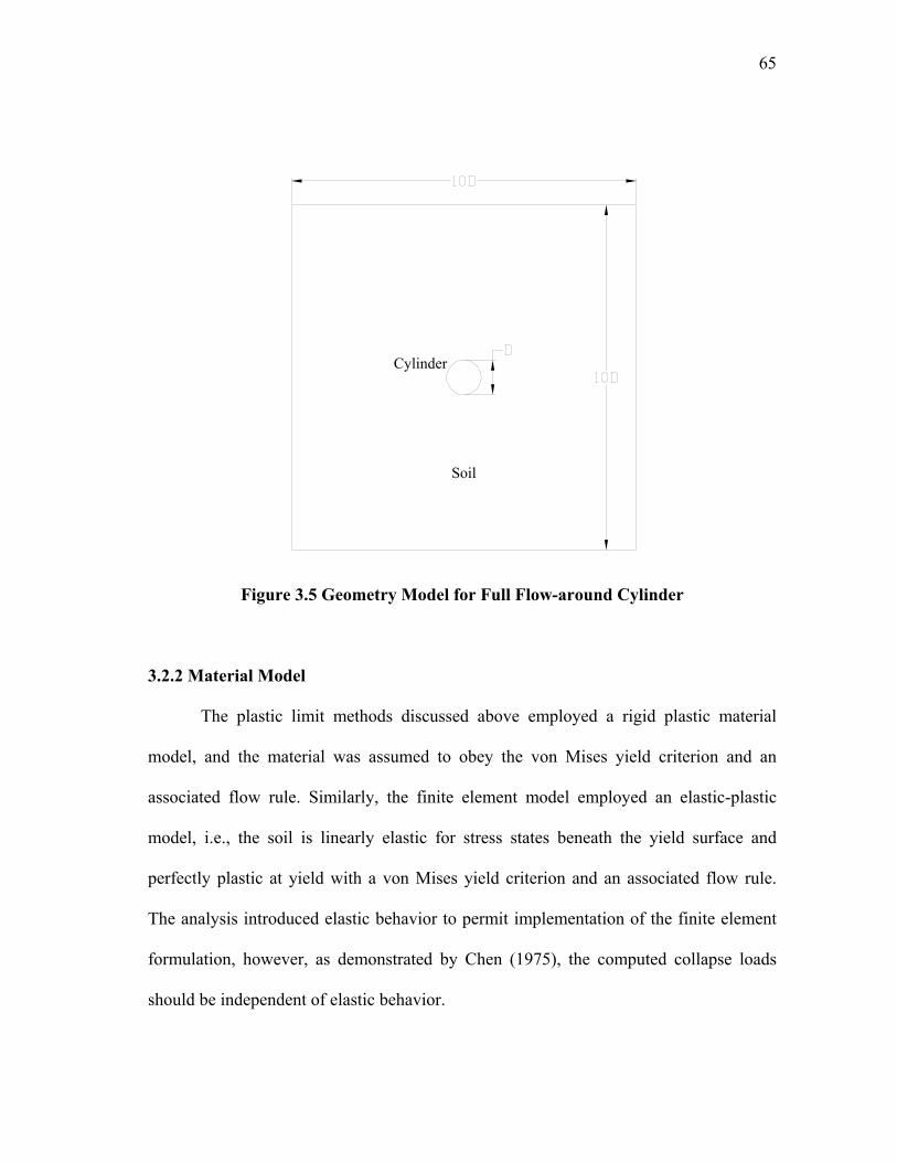
65

Soil

Cylinder

Figure 3.5 Geometry Model for Full Flow-around Cylinder

3.2.2 Material Model

The plastic limit methods discussed above employed a rigid plastic material

model, and the material was assumed to obey the von Mises yield criterion and an

associated flow rule. Similarly, the finite element model employed an elastic-plastic

model, i.e., the soil is linearly elastic for stress states beneath the yield surface and

perfectly plastic at yield with a von Mises yield criterion and an associated flow rule.

The analysis introduced elastic behavior to permit implementation of the finite element

formulation, however, as demonstrated by Chen (1975), the computed collapse loads

should be independent of elastic behavior.

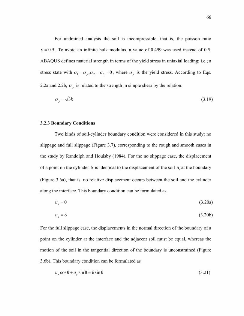
66

For undrained analysis the soil is incompressible, that is, the poisson ratio

0.5υ = . To avoid an infinite bulk modulus, a value of 0.499 was used instead of 0.5.

ABAQUS defines material strength in terms of the yield stress in uniaxial loading; i.e.; a

stress state with 1 2 3, 0yσ σ σ σ= = = , where yσ is the yield stress. According to Eqs.

2.2a and 2.2b, yσ is related to the strength in simple shear by the relation:

3y kσ = (3.19)

3.2.3 Boundary Conditions

Two kinds of soil-cylinder boundary condition were considered in this study: no

slippage and full slippage (Figure 3.7), corresponding to the rough and smooth cases in

the study by Randolph and Houlsby (1984). For the no slippage case, the displacement

of a point on the cylinder δ is identical to the displacement of the soil su at the boundary

(Figure 3.6a), that is, no relative displacement occurs between the soil and the cylinder

along the interface. This boundary condition can be formulated as

0xu = (3.20a)

δyu = (3.20b)

For the full slippage case, the displacements in the normal direction of the boundary of a

point on the cylinder at the interface and the adjacent soil must be equal, whereas the

motion of the soil in the tangential direction of the boundary is unconstrained (Figure

3.6b). This boundary condition can be formulated as

cosθ sinθ δsinθx yu u+ = (3.21)

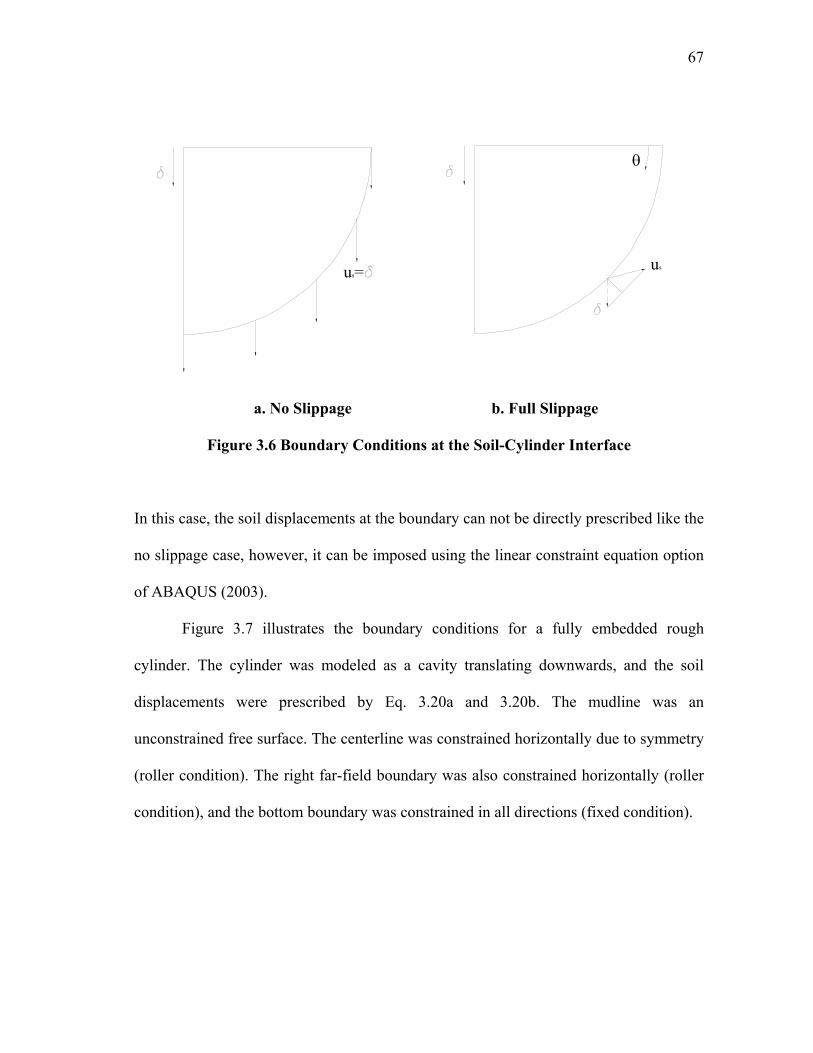
67

us=

θ

us

a. No Slippage b. Full Slippage

Figure 3.6 Boundary Conditions at the Soil-Cylinder Interface

In this case, the soil displacements at the boundary can not be directly prescribed like the

no slippage case, however, it can be imposed using the linear constraint equation option

of ABAQUS (2003).

Figure 3.7 illustrates the boundary conditions for a fully embedded rough

cylinder. The cylinder was modeled as a cavity translating downwards, and the soil

displacements were prescribed by Eq. 3.20a and 3.20b. The mudline was an

unconstrained free surface. The centerline was constrained horizontally due to symmetry

(roller condition). The right far-field boundary was also constrained horizontally (roller

condition), and the bottom boundary was constrained in all directions (fixed condition).

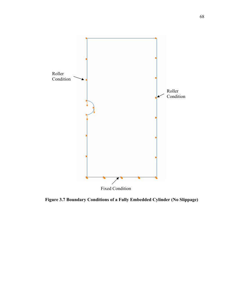
68

Figure 3.7 Boundary Conditions of a Fully Embedded Cylinder (No Slippage)

Roller Condition

Roller Condition

Fixed Condition

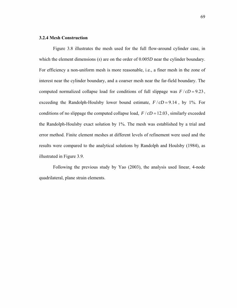
69

3.2.4 Mesh Construction

Figure 3.8 illustrates the mesh used for the full flow-around cylinder case, in

which the element dimensions (s) are on the order of 0.005D near the cylinder boundary.

For efficiency a non-uniform mesh is more reasonable, i.e., a finer mesh in the zone of

interest near the cylinder boundary, and a coarser mesh near the far-field boundary. The

computed normalized collapse load for conditions of full slippage was / 9.23F cD = ,

exceeding the Randolph-Houlsby lower bound estimate, / 9.14F cD = , by 1%. For

conditions of no slippage the computed collapse load, / 12.03F cD = , similarly exceeded

the Randolph-Houlsby exact solution by 1%. The mesh was established by a trial and

error method. Finite element meshes at different levels of refinement were used and the

results were compared to the analytical solutions by Randolph and Houlsby (1984), as

illustrated in Figure 3.9.

Following the previous study by Yao (2003), the analysis used linear, 4-node

quadrilateral, plane strain elements.

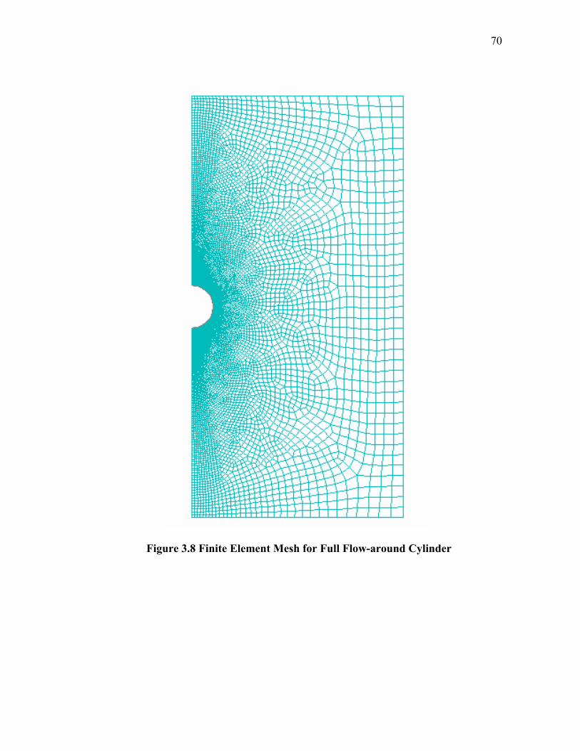
70

Figure 3.8 Finite Element Mesh for Full Flow-around Cylinder

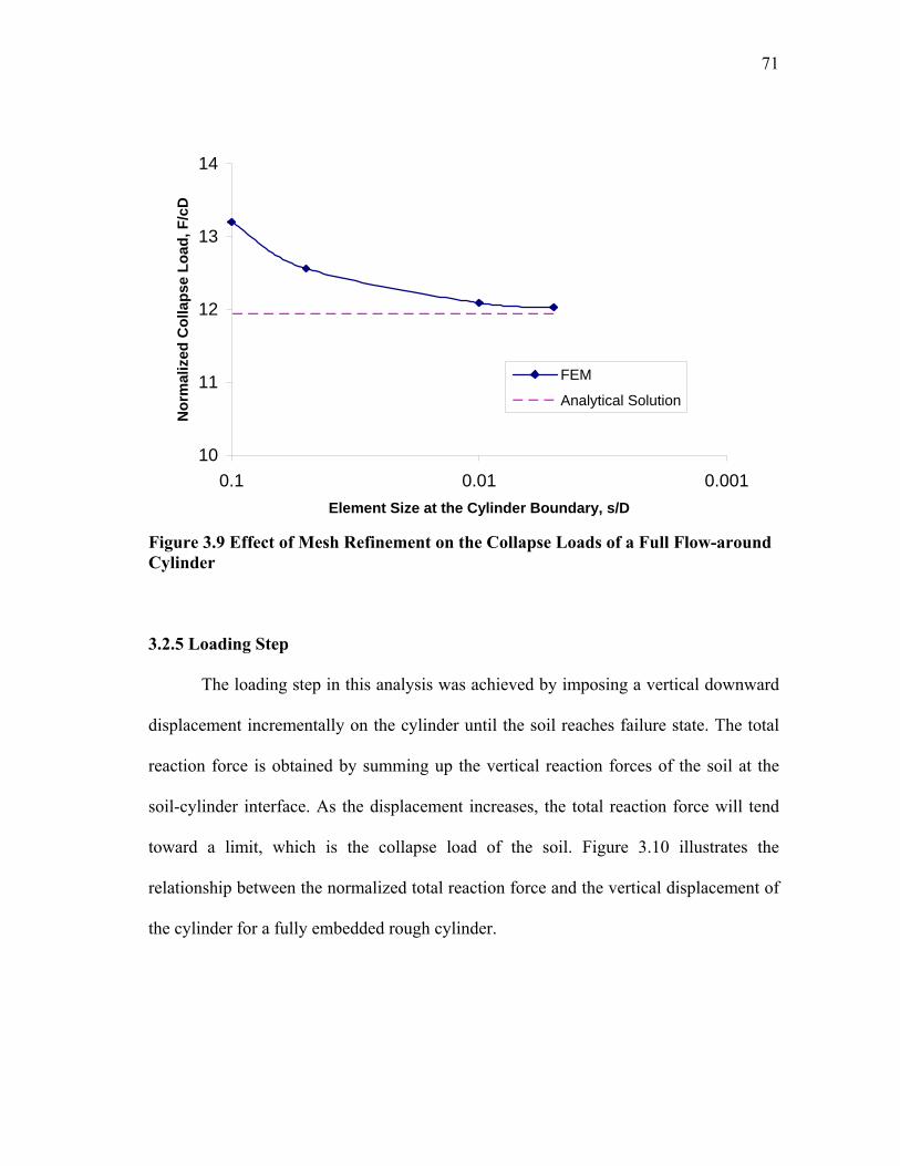
71

10

11

12

13

14

0.0010.010.1Element Size at the Cylinder Boundary, s/D

Nor

mal

ized

Col

laps

e Lo

ad, F

/cD

FEM

Analytical Solution

Figure 3.9 Effect of Mesh Refinement on the Collapse Loads of a Full Flow-around Cylinder

3.2.5 Loading Step

The loading step in this analysis was achieved by imposing a vertical downward

displacement incrementally on the cylinder until the soil reaches failure state. The total

reaction force is obtained by summing up the vertical reaction forces of the soil at the

soil-cylinder interface. As the displacement increases, the total reaction force will tend

toward a limit, which is the collapse load of the soil. Figure 3.10 illustrates the

relationship between the normalized total reaction force and the vertical displacement of

the cylinder for a fully embedded rough cylinder.

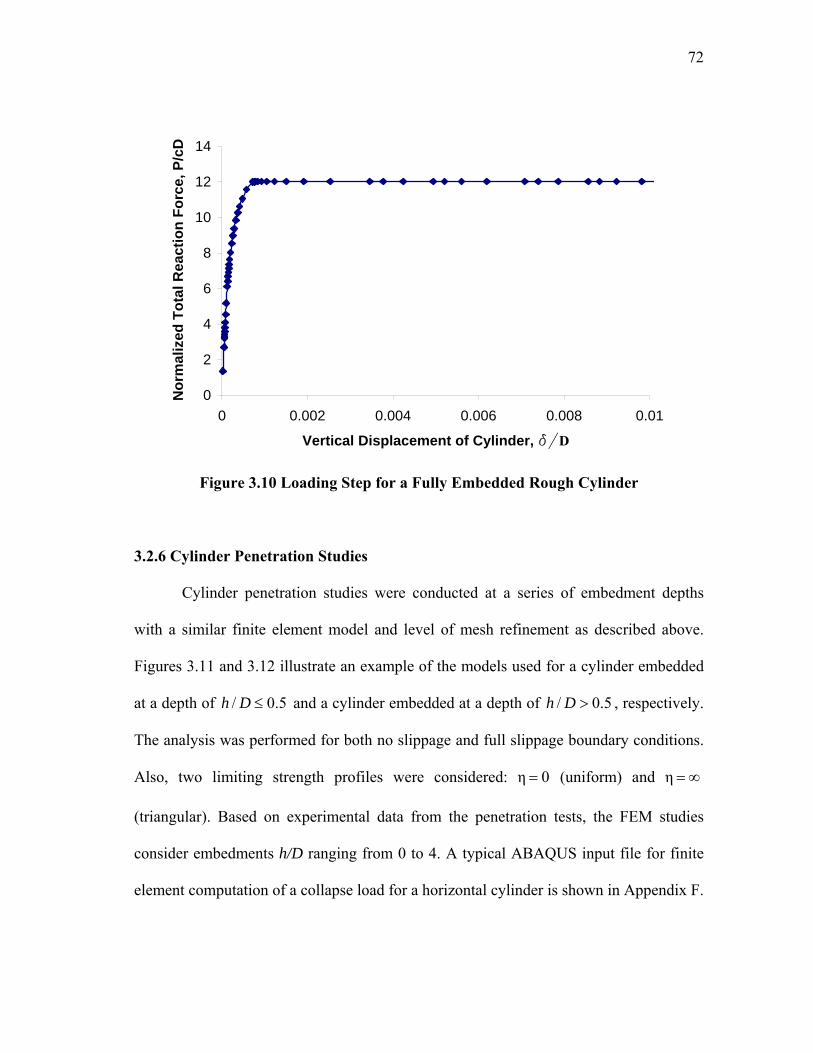
72

0

2

4

6

8

10

12

14

0 0.002 0.004 0.006 0.008 0.01

Vertical Displacement of Cylinder, d/D

Nor

mal

ized

Tot

al R

eact

ion

Forc

e, P

/cD

Figure 3.10 Loading Step for a Fully Embedded Rough Cylinder

3.2.6 Cylinder Penetration Studies

Cylinder penetration studies were conducted at a series of embedment depths

with a similar finite element model and level of mesh refinement as described above.

Figures 3.11 and 3.12 illustrate an example of the models used for a cylinder embedded

at a depth of / 0.5h D ≤ and a cylinder embedded at a depth of / 0.5h D > , respectively.

The analysis was performed for both no slippage and full slippage boundary conditions.

Also, two limiting strength profiles were considered: η 0= (uniform) and η = ∞

(triangular). Based on experimental data from the penetration tests, the FEM studies

consider embedments h/D ranging from 0 to 4. A typical ABAQUS input file for finite

element computation of a collapse load for a horizontal cylinder is shown in Appendix F.

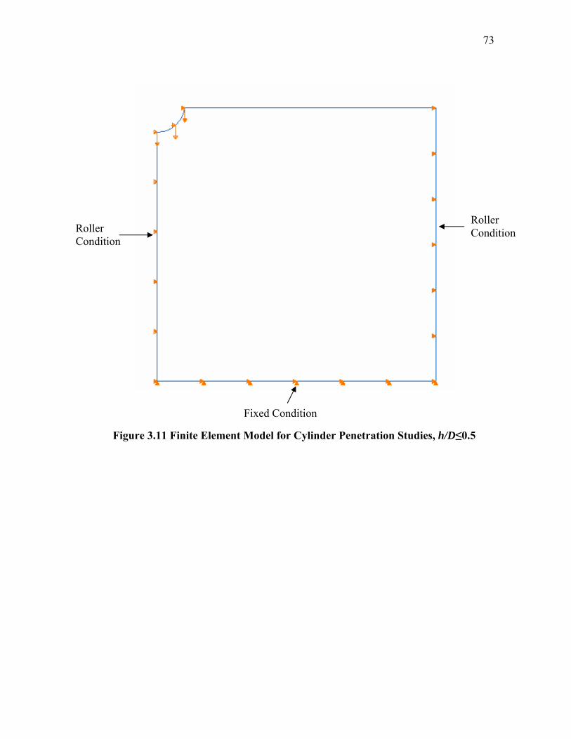
73

Figure 3.11 Finite Element Model for Cylinder Penetration Studies, h/D≤0.5

Roller Condition Roller

Condition

Fixed Condition

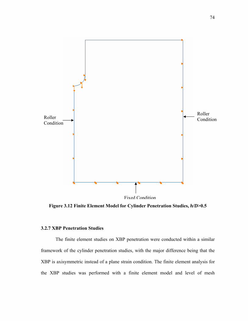
74

Figure 3.12 Finite Element Model for Cylinder Penetration Studies, h/D>0.5

3.2.7 XBP Penetration Studies

The finite element studies on XBP penetration were conducted within a similar

framework of the cylinder penetration studies, with the major difference being that the

XBP is axisymmetric instead of a plane strain condition. The finite element analysis for

the XBP studies was performed with a finite element model and level of mesh

Roller Condition Roller

Condition

Fixed Condition

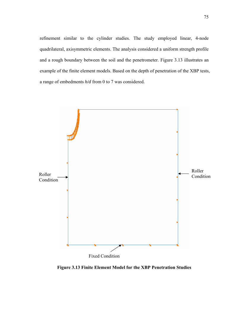
75

refinement similar to the cylinder studies. The study employed linear, 4-node

quadrilateral, axisymmetric elements. The analysis considered a uniform strength profile

and a rough boundary between the soil and the penetrometer. Figure 3.13 illustrates an

example of the finite element models. Based on the depth of penetration of the XBP tests,

a range of embedments h/d from 0 to 7 was considered.

Figure 3.13 Finite Element Model for the XBP Penetration Studies

Roller Condition Roller

Condition

Fixed Condition

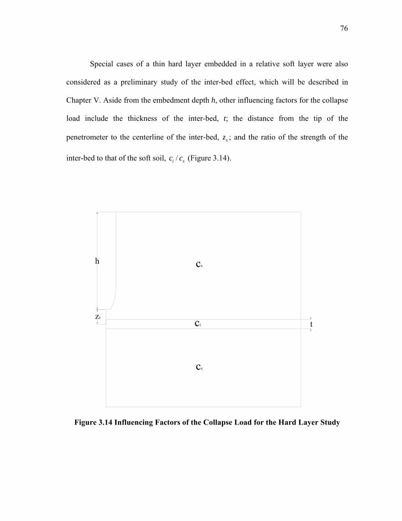
76

Special cases of a thin hard layer embedded in a relative soft layer were also

considered as a preliminary study of the inter-bed effect, which will be described in

Chapter V. Aside from the embedment depth h, other influencing factors for the collapse

load include the thickness of the inter-bed, t; the distance from the tip of the

penetrometer to the centerline of the inter-bed, sz ; and the ratio of the strength of the

inter-bed to that of the soft soil, /i sc c (Figure 3.14).

zs

t

h cs

cs

ci

Figure 3.14 Influencing Factors of the Collapse Load for the Hard Layer Study

77

3.3 Comparison of Solutions

Figures 3.15 and 3.16 compare finite element estimates of collapse loads of a

cylinder at shallow embedments ( / 0.5h D ≤ ) for various conditions of cylinder

boundary roughness and soil strength profiles to the plasticity solutions.

For a smooth cylinder with uniform soil strength conditions (Figure 3.15a), the

lower bound MOC solution is in close agreement with the finite element solution for

embedments h/D up to about 0.3. Beyond this depth the two solutions diverge somewhat

until at h/D=0.5 the finite element solution exceeds the lower bound estimate by about

10%. The consistent upper bound solution agrees with the finite element solution only

for very shallow embedments, h/D<0.1. At greater embedments, the consistent upper

bound solution increasingly diverges from the finite element solution, until at h/D=0.5 it

exceeds the finite element solution by about 25%. For embedments greater than h/D>0.3,

the upperbound derived from truncated Randolph-Houlsby velocity field is actually in

better agreement with the finite element solution than the consistent upperbound solution.

Figure 3.15b presents the case of a rough boundary and a uniform strength

profile. The consistent upperbound solution is in virtual perfect agreement with the finite

element solution for embedment depths up to h/D<0.3, diverging from the finite element

solution at greater embedments by up to 5%. The Randolph-Houlsby solution exceeds

the finite element solution by over 10% at shallow embedments, h/D<0.3. At greater

embedments the differences decline, until at one radius embedment, h/D=0.5, the two

solutions are in agreement.

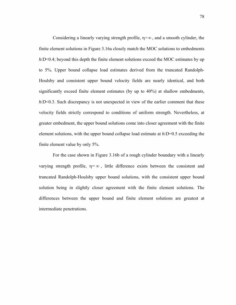
78

Considering a linearly varying strength profile, η= ∞ , and a smooth cylinder, the

finite element solutions in Figure 3.16a closely match the MOC solutions to embedments

h/D<0.4; beyond this depth the finite element solutions exceed the MOC estimates by up

to 5%. Upper bound collapse load estimates derived from the truncated Randolph-

Houlsby and consistent upper bound velocity fields are nearly identical, and both

significantly exceed finite element estimates (by up to 40%) at shallow embedments,

h/D<0.3. Such discrepancy is not unexpected in view of the earlier comment that these

velocity fields strictly correspond to conditions of uniform strength. Nevertheless, at

greater embedment, the upper bound solutions come into closer agreement with the finite

element solutions, with the upper bound collapse load estimate at h/D=0.5 exceeding the

finite element value by only 5%.

For the case shown in Figure 3.16b of a rough cylinder boundary with a linearly

varying strength profile, η= ∞ , little difference exists between the consistent and

truncated Randolph-Houlsby upper bound solutions, with the consistent upper bound

solution being in slightly closer agreement with the finite element solutions. The

differences between the upper bound and finite element solutions are greatest at

intermediate penetrations.

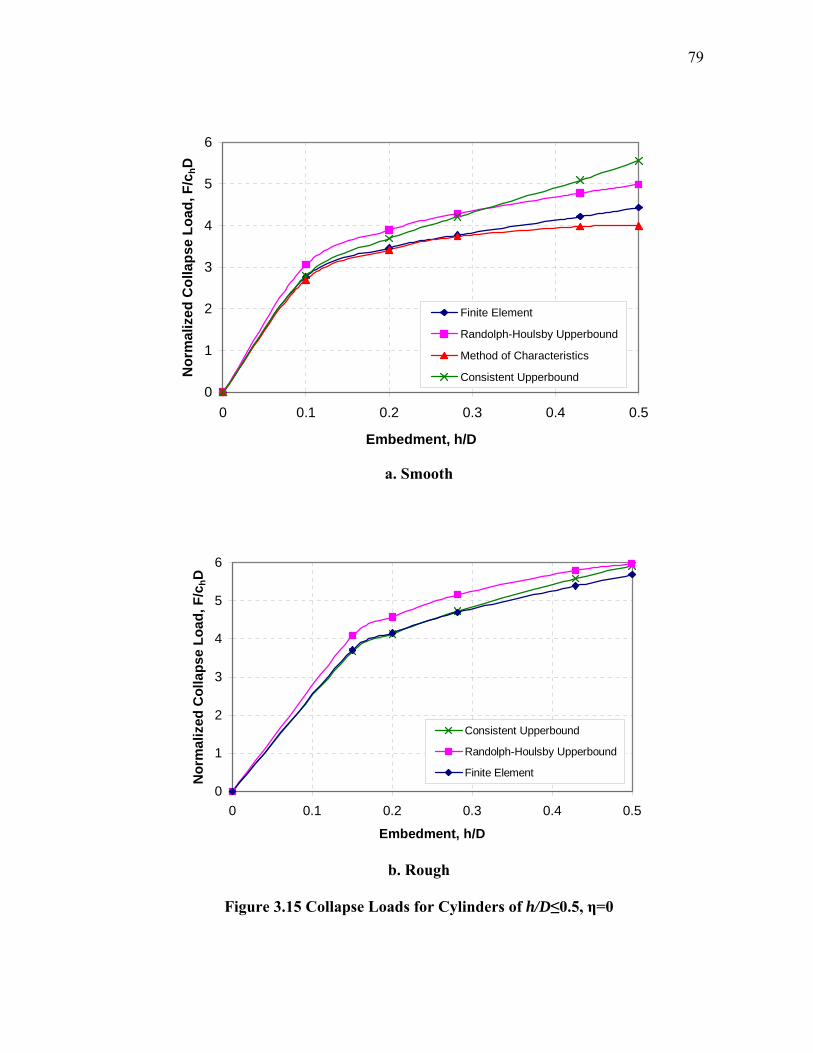
79

0

1

2

3

4

5

6

0 0.1 0.2 0.3 0.4 0.5

Embedment, h/D

Nor

mal

ized

Col

laps

e Lo

ad, F

/chD

Finite Element

Randolph-Houlsby Upperbound

Method of Characteristics

Consistent Upperbound

a. Smooth

0

1

2

3

4

5

6

0 0.1 0.2 0.3 0.4 0.5

Embedment, h/D

Nor

mal

ized

Col

laps

e Lo

ad, F

/chD

Consistent Upperbound

Randolph-Houlsby Upperbound

Finite Element

b. Rough

Figure 3.15 Collapse Loads for Cylinders of h/D≤0.5, η=0

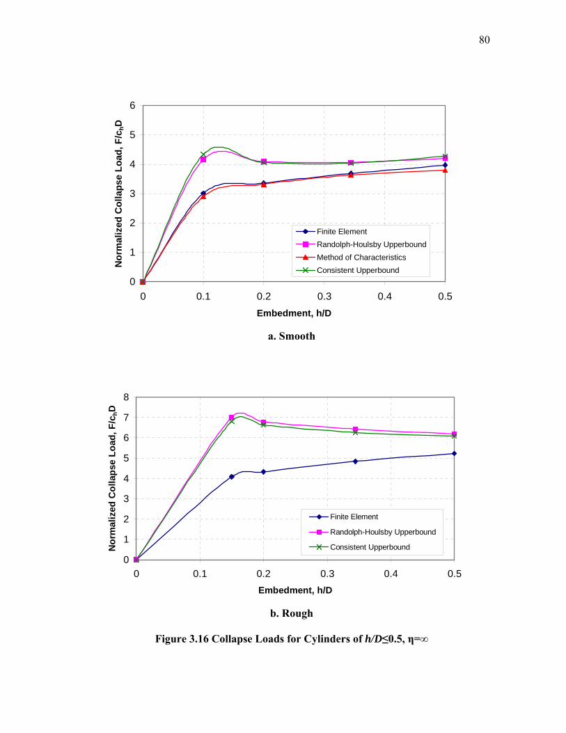
80

0

1

2

3

4

5

6

0 0.1 0.2 0.3 0.4 0.5Embedment, h/D

Nor

mal

ized

Col

laps

e Lo

ad, F

/chD

Finite ElementRandolph-Houlsby UpperboundMethod of CharacteristicsConsistent Upperbound

a. Smooth

0

1

2

3

4

5

6

7

8

0 0.1 0.2 0.3 0.4 0.5Embedment, h/D

Nor

mal

ized

Col

laps

e Lo

ad, F

/chD

Finite Element

Randolph-Houlsby Upperbound

Consistent Upperbound

b. Rough

Figure 3.16 Collapse Loads for Cylinders of h/D≤0.5, η=∞

81

Figures 3.17 and 3.18 compare finite element and upper bound solutions at

embedments of / 0.5h D > . Figure 3.17a compares solutions for uniform soil strength

profile and smooth cylinder boundary condition. The collapse loads predicted from the

upper bound solution increase rather abruptly between cylinder embedments 0.5<h/D<1,

beyond which they becomes constant. Such a trend is predictable for this presumed

failure mechanism, since no additional soil resistance can be mobilized once the

horizontal free surface lies above the slip line field boundary (Figure 3.4). The finite

element solution indicates the abrupt break in the upper bound solution (Figures 3.17a)

to be unrealistic. Refinement of the upper bound solution to allow the passive wedge to

exit at an optimized angle (Martin, 2001) could likely smooth these abrupt transitions.

The upper bound solution overestimates the finite element solution most severely - by

about 50%- at relatively low embedments in the range 1<h/D<2. At greater embedment

depths, the finite element predictions gradually trend toward the upper bound solution.

The upper bound solution for a smooth boundary and linearly varying strength profile,

η= ∞ , in Figure 3.18a begins to significantly diverge from the finite element solution at

embedments h/D>1. Beyond h/D>1.5, it roughly parallels the finite element solutions,

exceeding it by about 20%. The comparison of the upper bound solutions for a rough

boundary in Figures 3.17b and Figure 3.18b to the finite element solutions is similar to

that of the smooth case.

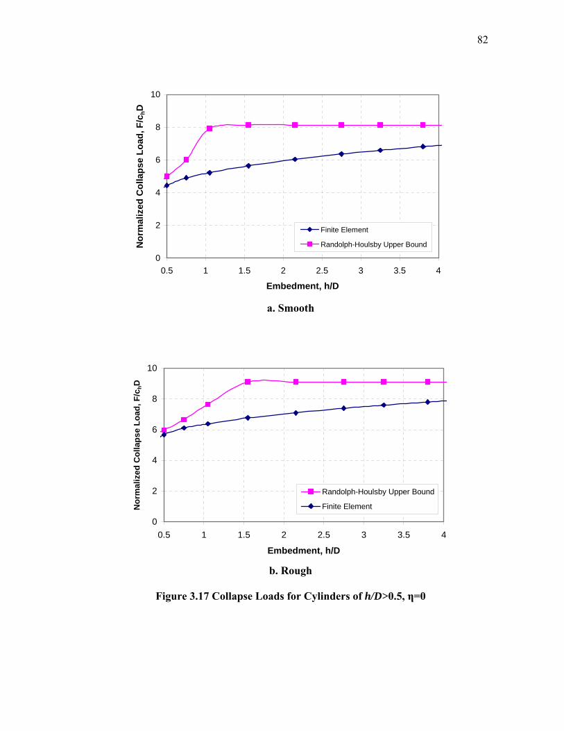
82

0

2

4

6

8

10

0.5 1 1.5 2 2.5 3 3.5 4

Embedment, h/D

Nor

mal

ized

Col

laps

e Lo

ad, F

/chD

Finite Element

Randolph-Houlsby Upper Bound

a. Smooth

0

2

4

6

8

10

0.5 1 1.5 2 2.5 3 3.5 4

Embedment, h/D

Nor

mal

ized

Col

laps

e Lo

ad, F

/chD

Randolph-Houlsby Upper Bound

Finite Element

b. Rough

Figure 3.17 Collapse Loads for Cylinders of h/D>0.5, η=0

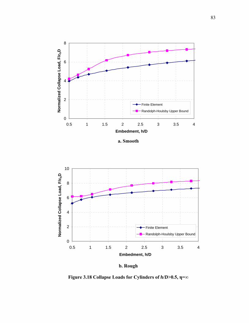
83

0

2

4

6

8

0.5 1 1.5 2 2.5 3 3.5 4

Embedment, h/D

Nor

mal

ized

Col

laps

e Lo

ad, F

/chD

Finite Element

Randolph-Houlsby Upper Bound

a. Smooth

0

2

4

6

8

10

0.5 1 1.5 2 2.5 3 3.5 4

Embedment, h/D

Nor

mal

ized

Col

laps

e Lo

ad, F

/chD

Finite Element

Randolph-Houlsby Upper Bound

b. Rough

Figure 3.18 Collapse Loads for Cylinders of h/D>0.5, η=∞

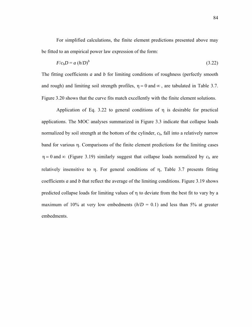
84

For simplified calculations, the finite element predictions presented above may

be fitted to an empirical power law expression of the form:

F/chD = a (h/D)b (3.22)

The fitting coefficients a and b for limiting conditions of roughness (perfectly smooth

and rough) and limiting soil strength profiles, ∞= and0η , are tabulated in Table 3.7.

Figure 3.20 shows that the curve fits match excellently with the finite element solutions.

Application of Eq. 3.22 to general conditions of η is desirable for practical

applications. The MOC analyses summarized in Figure 3.3 indicate that collapse loads

normalized by soil strength at the bottom of the cylinder, ch, fall into a relatively narrow

band for various η. Comparisons of the finite element predictions for the limiting cases

∞= and0η (Figure 3.19) similarly suggest that collapse loads normalized by ch are

relatively insensitive to η. For general conditions of η, Table 3.7 presents fitting

coefficients a and b that reflect the average of the limiting conditions. Figure 3.19 shows

predicted collapse loads for limiting values of η to deviate from the best fit to vary by a

maximum of 10% at very low embedments (h/D = 0.1) and less than 5% at greater

embedments.

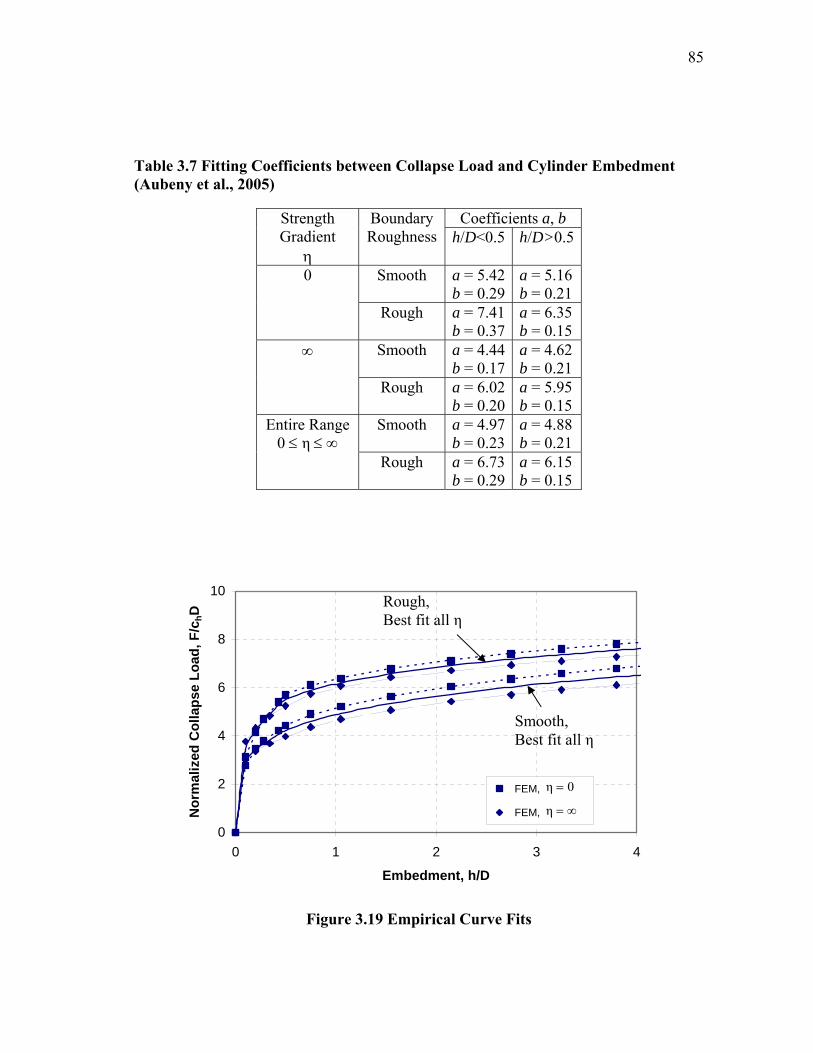
85

Table 3.7 Fitting Coefficients between Collapse Load and Cylinder Embedment (Aubeny et al., 2005)

0

2

4

6

8

10

0 1 2 3 4

Embedment, h/D

Nor

mal

ized

Col

laps

e Lo

ad, F

/chD

FEM,

FEM,

Figure 3.19 Empirical Curve Fits

Coefficients a, b Strength Gradient

η

Boundary Roughness h/D<0.5 h/D>0.5

Smooth a = 5.42b = 0.29

a = 5.16 b = 0.21

0

Rough a = 7.41b = 0.37

a = 6.35 b = 0.15

Smooth a = 4.44 b = 0.17

a = 4.62 b = 0.21

∞

Rough a = 6.02b = 0.20

a = 5.95 b = 0.15

Smooth a = 4.97b = 0.23

a = 4.88 b = 0.21

Entire Range ∞≤≤ η0

Rough a = 6.73b = 0.29

a = 6.15 b = 0.15

η 0

η

=

= ∞

Rough, Best fit all η

Smooth, Best fit all η

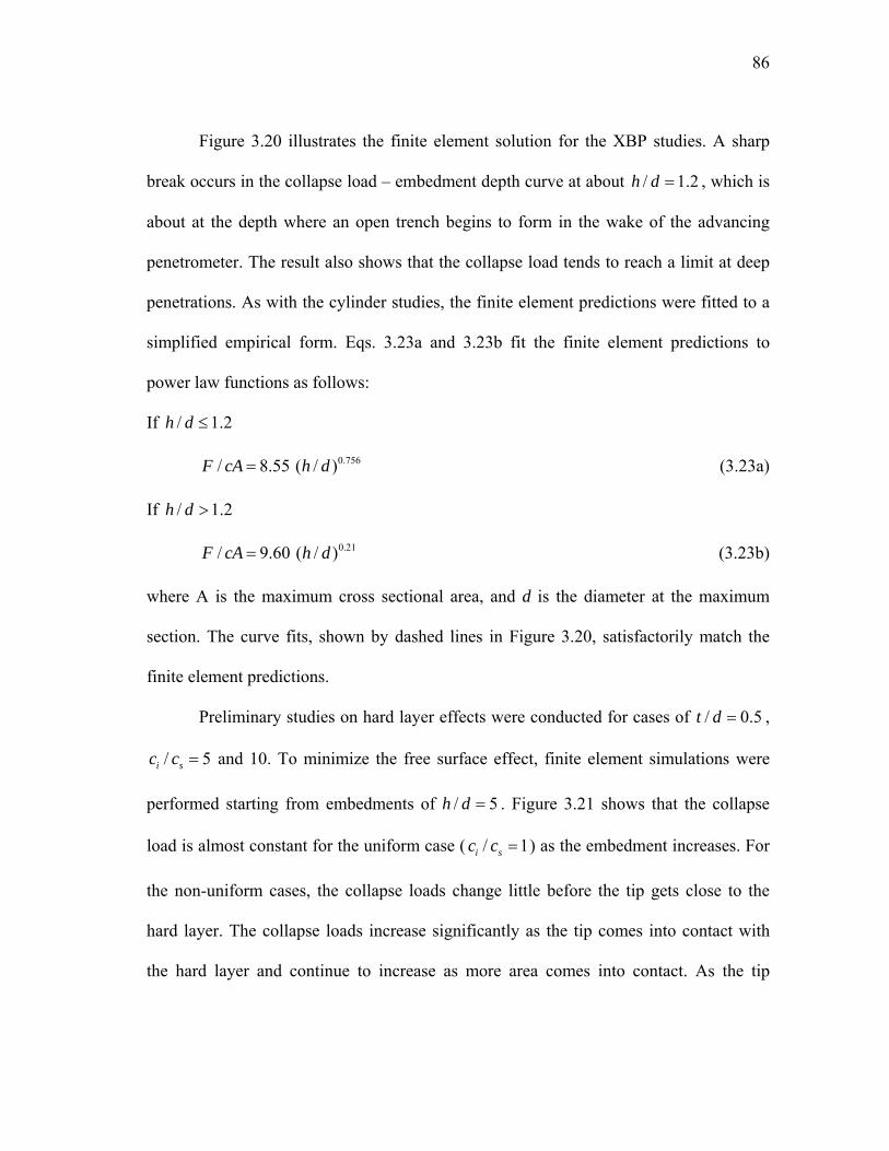
86

Figure 3.20 illustrates the finite element solution for the XBP studies. A sharp

break occurs in the collapse load – embedment depth curve at about / 1.2h d = , which is

about at the depth where an open trench begins to form in the wake of the advancing

penetrometer. The result also shows that the collapse load tends to reach a limit at deep

penetrations. As with the cylinder studies, the finite element predictions were fitted to a

simplified empirical form. Eqs. 3.23a and 3.23b fit the finite element predictions to

power law functions as follows:

If / 1.2h d ≤

0.756/ 8.55 ( / )F cA h d= (3.23a)

If / 1.2h d >

0.21/ 9.60 ( / )F cA h d= (3.23b)

where A is the maximum cross sectional area, and d is the diameter at the maximum

section. The curve fits, shown by dashed lines in Figure 3.20, satisfactorily match the

finite element predictions.

Preliminary studies on hard layer effects were conducted for cases of / 0.5t d = ,

/ 5i sc c = and 10. To minimize the free surface effect, finite element simulations were

performed starting from embedments of / 5h d = . Figure 3.21 shows that the collapse

load is almost constant for the uniform case ( / 1i sc c = ) as the embedment increases. For

the non-uniform cases, the collapse loads change little before the tip gets close to the

hard layer. The collapse loads increase significantly as the tip comes into contact with

the hard layer and continue to increase as more area comes into contact. As the tip

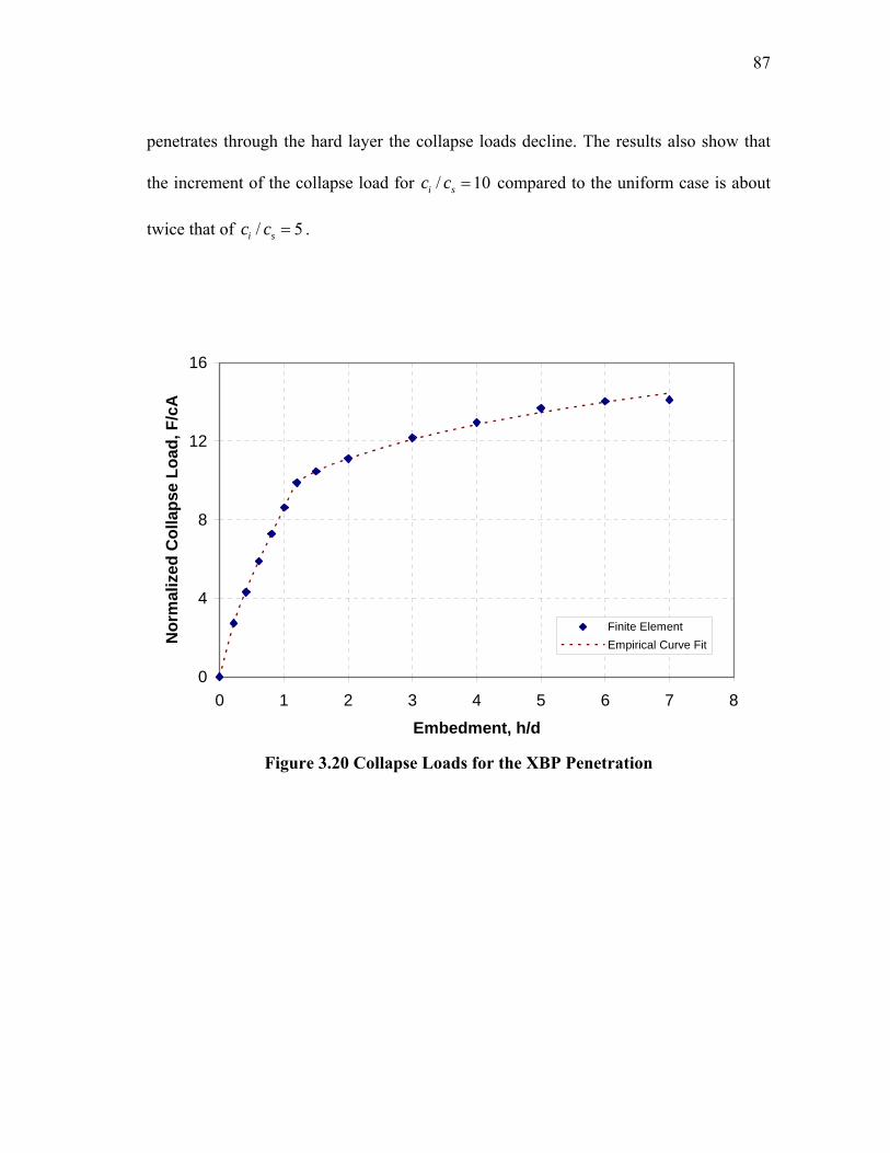
87

penetrates through the hard layer the collapse loads decline. The results also show that

the increment of the collapse load for / 10i sc c = compared to the uniform case is about

twice that of / 5i sc c = .

0

4

8

12

16

0 1 2 3 4 5 6 7 8

Embedment, h/d

Nor

mal

ized

Col

laps

e Lo

ad, F

/cA

Finite ElementEmpirical Curve Fit

Figure 3.20 Collapse Loads for the XBP Penetration

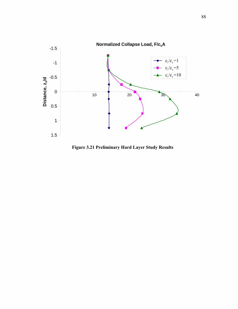
88

-1.5

-1

-0.5

0

0.5

1

1.5

Normalized Collapse Load, F/csAD

ista

nce,

zs/d

Figure 3.21 Preliminary Hard Layer Study Results

i s

i s

i s

c /c =1c /c =5c /c =10

10 4020 30

89

CHAPTER IV

RATE-DEPENDENT STUDIES

4.1 Rate-Dependent Strength Model

The dependence of undrained shear strength on strain rate may be characterized

in terms of a semi-logarithmic relation:

( )101 ρ log ε / εref ref refc c ⎡ ⎤= +⎣ ⎦ (4.1)

where c = undrained shear strength at strain rate ε

refc = undrained shear strength at reference strain rateεref

ρref = strain rate parameter associated with the reference strain rate εref

Data by Sheahan et al. (1996) suggest the existence of a threshold strain rate, 0ε ,

below which strain rate effects are negligible. In re-sedimented Boston Blue Clay,

reported threshold strain rates were 0.5 and 5%/hr for over-consolidation ratios (OCR) of

4 and 8, respectively. For lower OCR, thresholds were not encountered for strain rates

down to 0.05%/hr. Hence, for normally and lightly over-consolidated soils, the lower

limit of strain rate, or threshold strain rate for which Eq. 4.1 is valid, is a matter of some

uncertainty. The maximum strain rates investigated in previously reported investigations

are typically on the order of 50%/hr (Sheahan et al., 1996), with a single study

considering strain rates up to 670%/hr (Vaid and Campanella, 1977).

Having noted the considerable uncertainty in the range of strain rates for which

Eq. 4.1 is valid for normally consolidated clays, the following assumptions were made

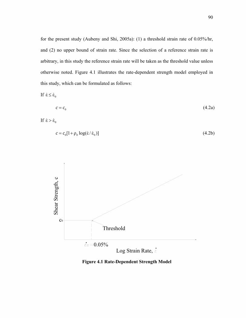
90

for the present study (Aubeny and Shi, 2005a): (1) a threshold strain rate of 0.05%/hr,

and (2) no upper bound of strain rate. Since the selection of a reference strain rate is

arbitrary, in this study the reference strain rate will be taken as the threshold value unless

otherwise noted. Figure 4.1 illustrates the rate-dependent strength model employed in

this study, which can be formulated as follows:

If 0ε ε≤

0c c= (4.2a)

If 0ε ε>

0 0 0[1 ρ log(ε / ε )]c c= + (4.2b)

Shea

r Stre

ngth

, c

Log Strain Rate, .0.05%

Thresholdc0

.

Figure 4.1 Rate-Dependent Strength Model

91

The data by Sheahan (1996) also show that ρref is not in general constant, but tends to

increase with increasing strain rate; i.e., soil shearing resistance actually increases at a

rate greater than that predicted from the simple semi-logarithmic law in Eq. 4.1. Data

from miniature vane shear tests conducted at variable vane peripheral velocities

(Biscontin and Pestana, 2001) indicate a similar trend.

4.2 Finite Element Studies for Cylinders

Eq. 4.1 describes rate dependent soil resistance at a point. To characterize the

total soil shearing resistance Fs of a cylinder of diameter D at an instantaneous velocity

v, an analogous equation may be considered (Aubeny and Shi, 2005a):

( )s s0 0 10 01 λ log / εF F v D= +⎡ ⎤⎣ ⎦ (4.3)

The threshold soil resistance 0sF in Eq. 4.3 is the quasi-static soil shearing

resisting force computed using a soil strength corresponding to the threshold strain rate

0ε , and 0λ is the strain rate multiplier for a cylinder embedded in a trench. The strain

rate parameter 0λ is analogous to the parameter 0ρ in Eq. 4.2b; however, the existence

of a threshold strain rate below which strength remains constant precludes the possibility

that 0λ may be identically equal to 0ρ . The first objective of the finite element studies is,

therefore, to evaluate 0λ in relation to 0ρ for various conditions of (1) dimensionless

velocity v/D 0ε , (2) dimensionless penetration h/D. The second objective is to evaluate

the accuracy of applying Eq. 3.22 to Eq. 4.3 in obtaining estimates of the soil resisting

force Fs corresponding to penetration velocity v. For the purposes of the mine impact

92

penetration investigations that motivated this research, a range of dimensionless

velocities v/D 0ε up to 109 are taken as the range of interest.

4.2.1 Finite Element Model

The rate-dependent finite element analysis used the same geometry model, finite

element mesh and element type as the rate-independent studies. The boundary conditions

are also the same, except that the cylinder was modeled as a circular cavity translating

downward at a constant velocity v instead of a prescribed displacement.

The soil was modeled as a rate-dependent, isotropic hardening material with a

von Mises yield criterion and associated flow rule. This is possible by using the “RATE

DEPENDENT, TYPE=YIELD RATIO” option together with the “PLASTIC,

HARDENING=ISOTROPIC” option in ABAQUS. The yield ratio is defined as

0σ σ (ε)y y R= (4.4)

where σ y is the yield stress at strain rate ε , 0σ y is the static yield stress, and R is the

yield ratio at strain rate ε . For a von Mises yield criterion, the yield stress is 3 times

the strength in simple shear. Combining with Eq. 4.2a and Eq. 4.2b we have

If 0ε ε≤

(ε) 1R = (4.5a)

If 0ε ε>

0 0(ε) 1 ρ log(ε / ε )R = + (4.5b)

93

The loading step is similar with that of the rate-independent study, i.e., the

collapse load is achieved when the cylinder moves at a certain displacement. However,

since we prescribe velocity instead of displacement in this case, ABAQUS calculates a

displacement increment by multiplying the velocity of the cylinder by the time

increment.

4.2.2 Finite Element Results

Figure 4.2 illustrates the effects of rate-dependent shear strength for velocities

v/D 0ε of 0 through 109 for a cylinder embedded at a depth h/D =2.15 with a strain rate

multiplier 0ρ 0.15= . This figure shows the magnitude of 2J (where J2 is the second

invariant of the deviatoric stress tensor) along the centerline beneath the cylinder for

collapse loading conditions. Recalling that the von Mises yield condition is 1/ 22 0J k− = ,

the calculated 2J is normalized by the static soil strength 0k to evaluate the strain rate

effects.

The predictions show that for quasi-static conditions, v/D 0ε = 0, the elasto-

plastic boundary occurs at a depth of about z/d = 3.1 below the bottom of the cylinder

and the mobilized shearing resistance is essentially constant within the plastic region. In

contrast, for “high” penetration velocities, say v/D 0ε > 103, the yielded region is slightly

expanded, with the elasto-plastic boundary occurring at about z/D = 3.6-3.8. Further, the

mobilized shearing resistance increases substantially within the yielded region in the

vicinity of the cylinder boundary due to the variable strain rates that occur within this

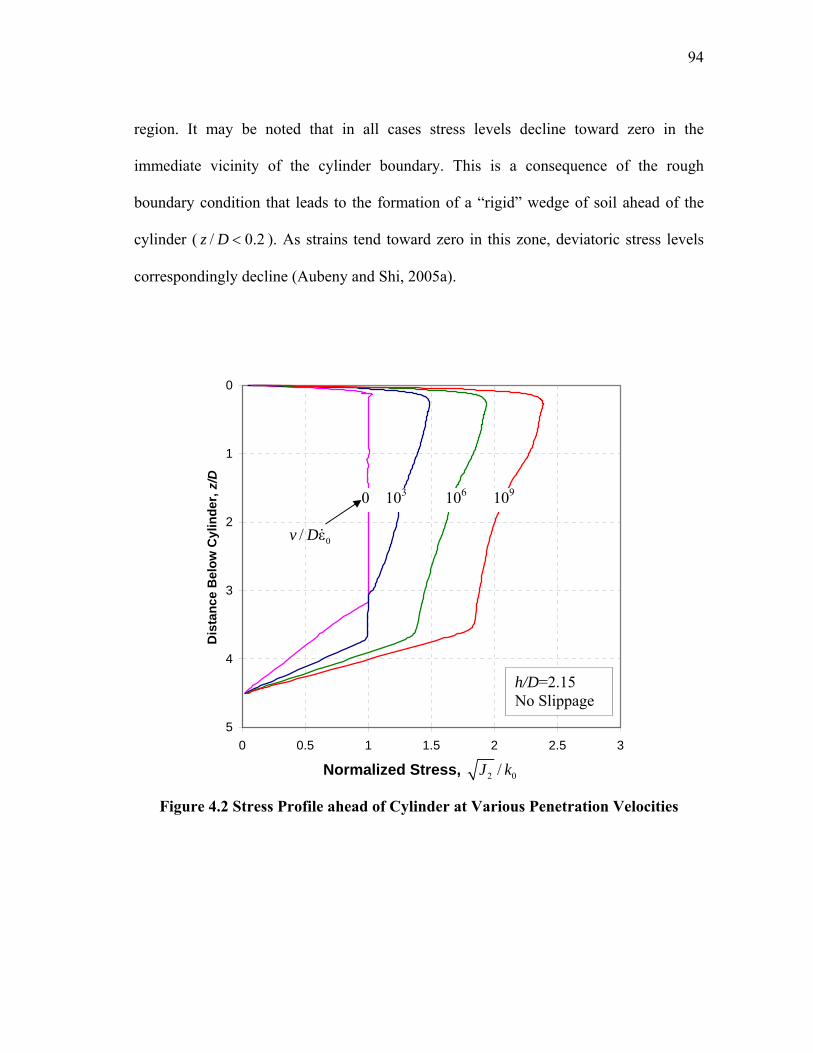
94

region. It may be noted that in all cases stress levels decline toward zero in the

immediate vicinity of the cylinder boundary. This is a consequence of the rough

boundary condition that leads to the formation of a “rigid” wedge of soil ahead of the

cylinder ( / 0.2z D < ). As strains tend toward zero in this zone, deviatoric stress levels

correspondingly decline (Aubeny and Shi, 2005a).

0

1

2

3

4

50 0.5 1 1.5 2 2.5 3

Dis

tanc

e B

elow

Cyl

inde

r, z/

D

Figure 4.2 Stress Profile ahead of Cylinder at Various Penetration Velocities

0/ εv D

0 103 106 109

Normalized Stress, 2 0/J k

h/D=2.15 No Slippage

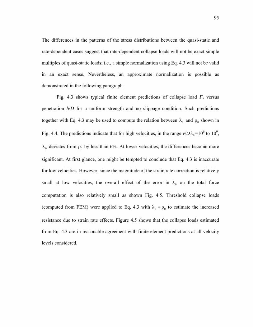
95

The differences in the patterns of the stress distributions between the quasi-static and

rate-dependent cases suggest that rate-dependent collapse loads will not be exact simple

multiples of quasi-static loads; i.e., a simple normalization using Eq. 4.3 will not be valid

in an exact sense. Nevertheless, an approximate normalization is possible as

demonstrated in the following paragraph.

Fig. 4.3 shows typical finite element predictions of collapse load Fs versus

penetration h/D for a uniform strength and no slippage condition. Such predictions

together with Eq. 4.3 may be used to compute the relation between 0λ and 0ρ shown in

Fig. 4.4. The predictions indicate that for high velocities, in the range v/D 0ε =106 to 109,

0λ deviates from 0ρ by less than 6%. At lower velocities, the differences become more

significant. At first glance, one might be tempted to conclude that Eq. 4.3 is inaccurate

for low velocities. However, since the magnitude of the strain rate correction is relatively

small at low velocities, the overall effect of the error in 0λ on the total force

computation is also relatively small as shown Fig. 4.5. Threshold collapse loads

(computed from FEM) were applied to Eq. 4.3 with 0 0λ ρ= to estimate the increased

resistance due to strain rate effects. Figure 4.5 shows that the collapse loads estimated

from Eq. 4.3 are in reasonable agreement with finite element predictions at all velocity

levels considered.

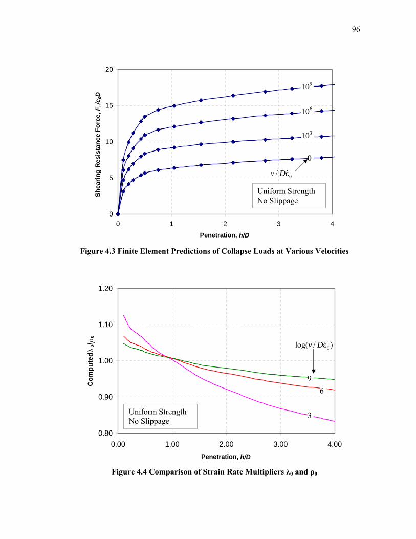
96

0

5

10

15

20

0 1 2 3 4Penetration, h/D

Shea

ring

Res

ista

nce

Forc

e, F

s/c0D

Figure 4.3 Finite Element Predictions of Collapse Loads at Various Velocities

0.80

0.90

1.00

1.10

1.20

0.00 1.00 2.00 3.00 4.00Penetration, h/D

Com

pute

d l0/ r

0

Figure 4.4 Comparison of Strain Rate Multipliers λ0 and ρ0

0log( / ε )v D

9 6

3 Uniform Strength No Slippage

0/ εv D

0

103

106

109

Uniform Strength No Slippage

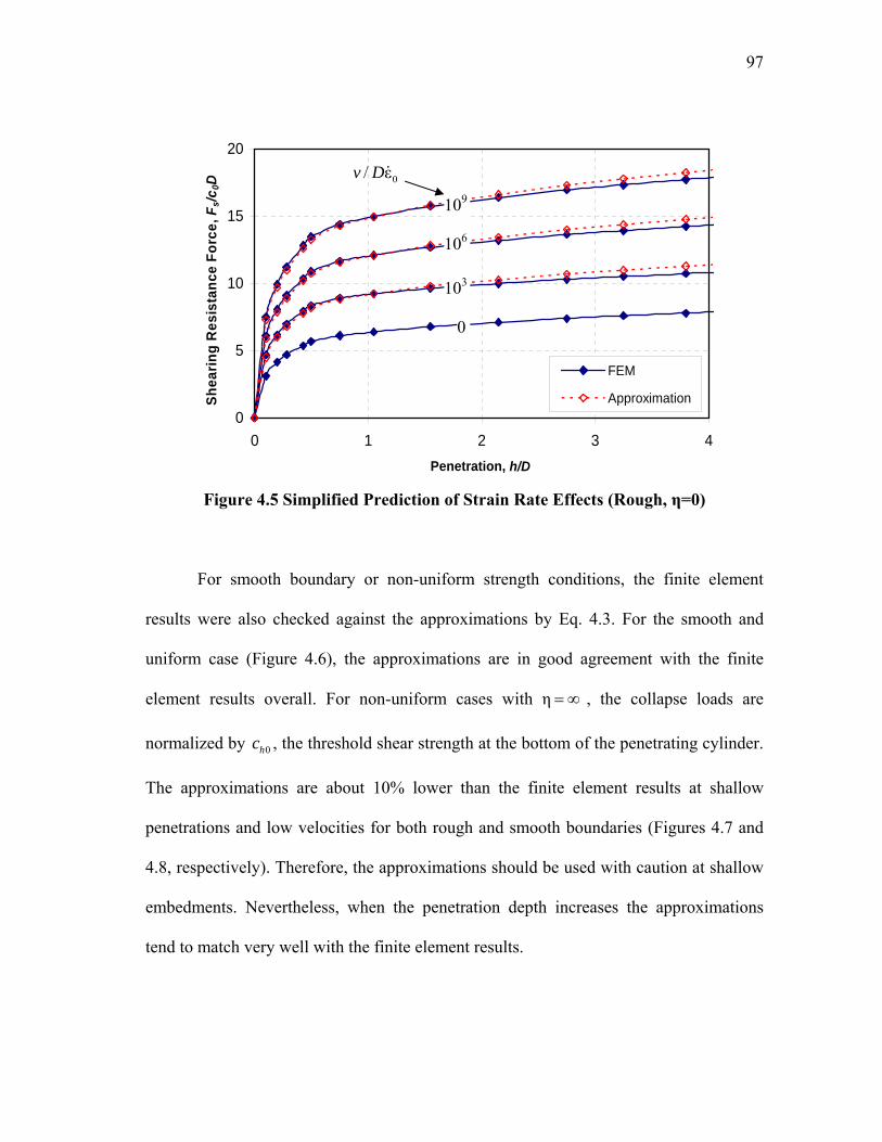
97

0

5

10

15

20

0 1 2 3 4Penetration, h/D

Shea

ring

Res

ista

nce

Forc

e, F

s/c0D

FEM

Approximation

Figure 4.5 Simplified Prediction of Strain Rate Effects (Rough, η=0)

For smooth boundary or non-uniform strength conditions, the finite element

results were also checked against the approximations by Eq. 4.3. For the smooth and

uniform case (Figure 4.6), the approximations are in good agreement with the finite

element results overall. For non-uniform cases with η = ∞ , the collapse loads are

normalized by 0hc , the threshold shear strength at the bottom of the penetrating cylinder.

The approximations are about 10% lower than the finite element results at shallow

penetrations and low velocities for both rough and smooth boundaries (Figures 4.7 and

4.8, respectively). Therefore, the approximations should be used with caution at shallow

embedments. Nevertheless, when the penetration depth increases the approximations

tend to match very well with the finite element results.

0/ εv D

0

103

106

109

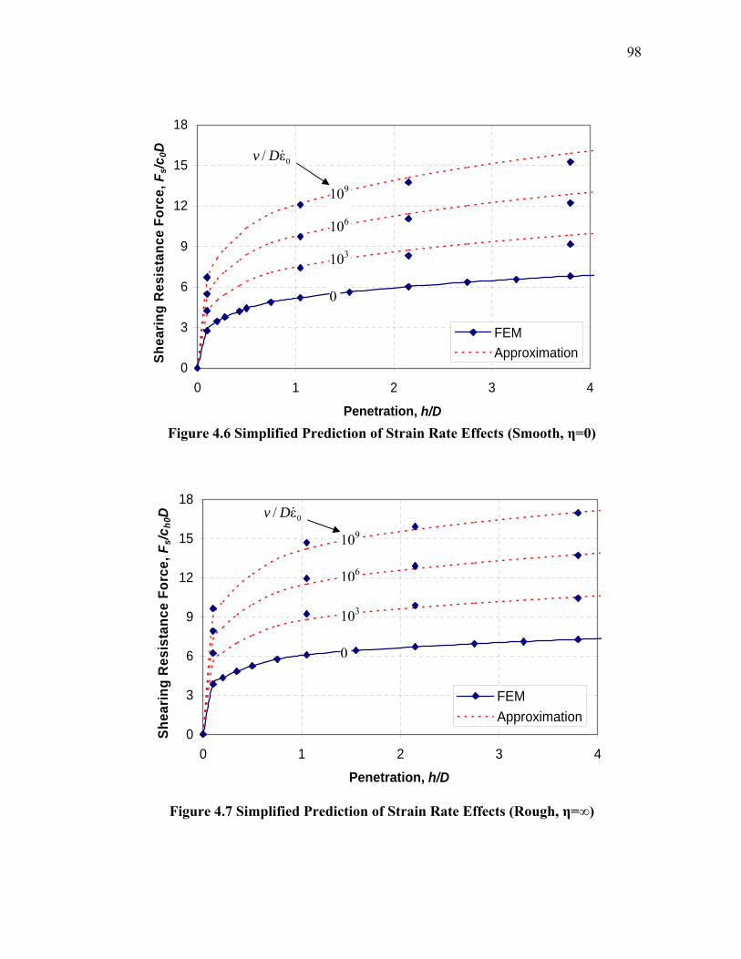
98

0

3

6

9

12

15

18

0 1 2 3 4

Penetration, h/D

Shea

ring

Res

ista

nce

Forc

e, F

s/c0D

FEMApproximation

Figure 4.6 Simplified Prediction of Strain Rate Effects (Smooth, η=0)

0

3

6

9

12

15

18

0 1 2 3 4

Penetration, h/D

Shea

ring

Res

ista

nce

Forc

e, F

s/ch0

D

FEMApproximation

Figure 4.7 Simplified Prediction of Strain Rate Effects (Rough, η=∞)

0/ εv D

109

106

103

0

109

106

103

0

0/ εv D

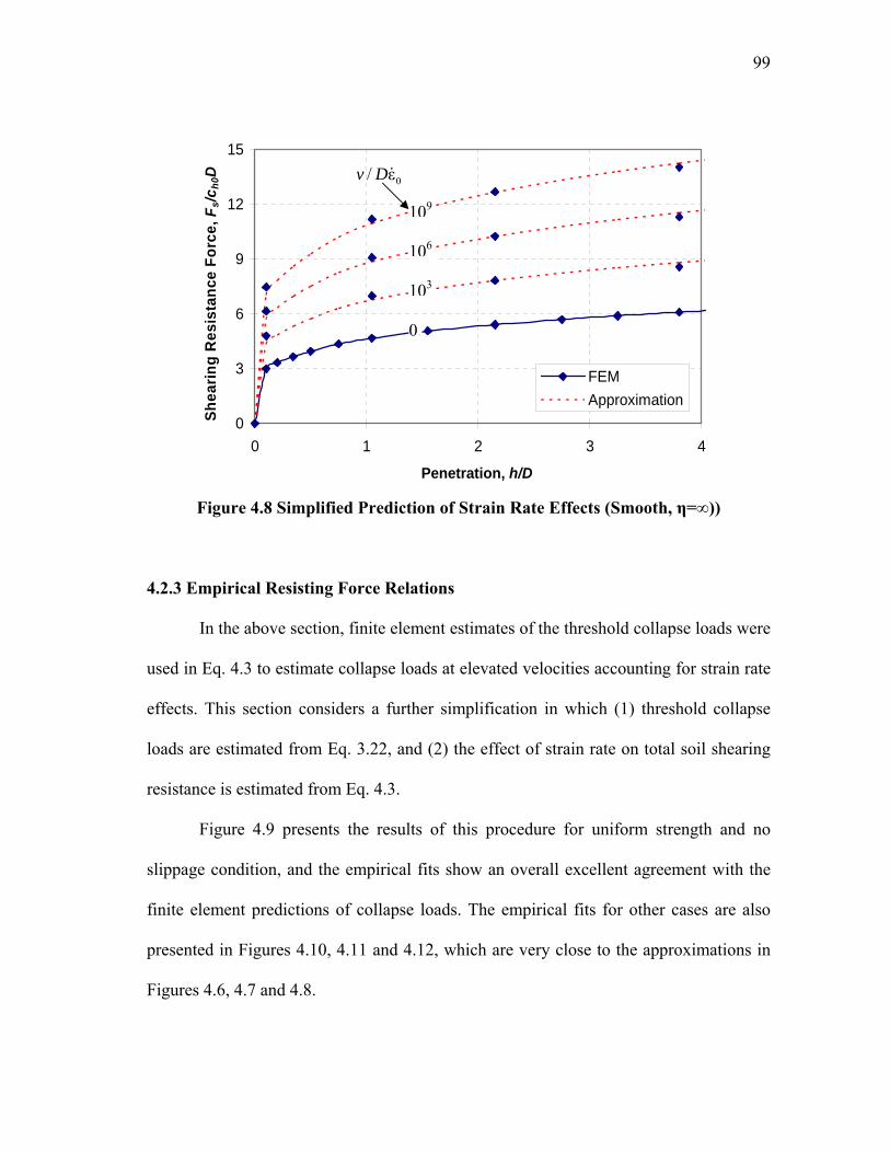
99

0

3

6

9

12

15

0 1 2 3 4

Penetration, h/D

Shea

ring

Res

ista

nce

Forc

e, F

s/ch0

D

FEMApproximation

Figure 4.8 Simplified Prediction of Strain Rate Effects (Smooth, η=∞))

4.2.3 Empirical Resisting Force Relations

In the above section, finite element estimates of the threshold collapse loads were

used in Eq. 4.3 to estimate collapse loads at elevated velocities accounting for strain rate

effects. This section considers a further simplification in which (1) threshold collapse

loads are estimated from Eq. 3.22, and (2) the effect of strain rate on total soil shearing

resistance is estimated from Eq. 4.3.

Figure 4.9 presents the results of this procedure for uniform strength and no

slippage condition, and the empirical fits show an overall excellent agreement with the

finite element predictions of collapse loads. The empirical fits for other cases are also

presented in Figures 4.10, 4.11 and 4.12, which are very close to the approximations in

Figures 4.6, 4.7 and 4.8.

0/ εv D

109

106

103

0

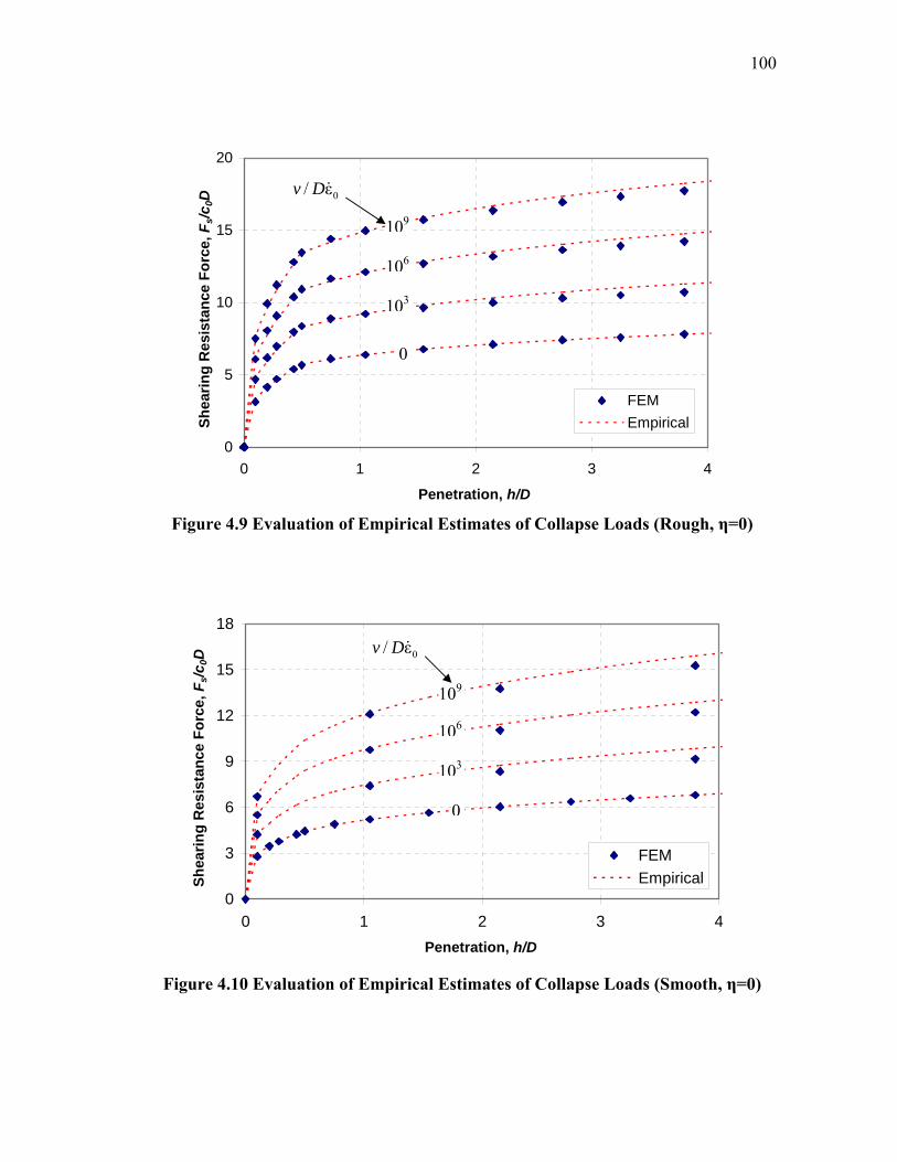
100

0

5

10

15

20

0 1 2 3 4

Penetration, h/D

Shea

ring

Res

ista

nce

Forc

e, F

s/c0D

FEMEmpirical

Figure 4.9 Evaluation of Empirical Estimates of Collapse Loads (Rough, η=0)

0

3

6

9

12

15

18

0 1 2 3 4Penetration, h/D

Shea

ring

Res

ista

nce

Forc

e, F

s/c0D

FEMEmpirical

Figure 4.10 Evaluation of Empirical Estimates of Collapse Loads (Smooth, η=0)

0/ εv D

109

106

103

0

0/ εv D

109

106

103

0

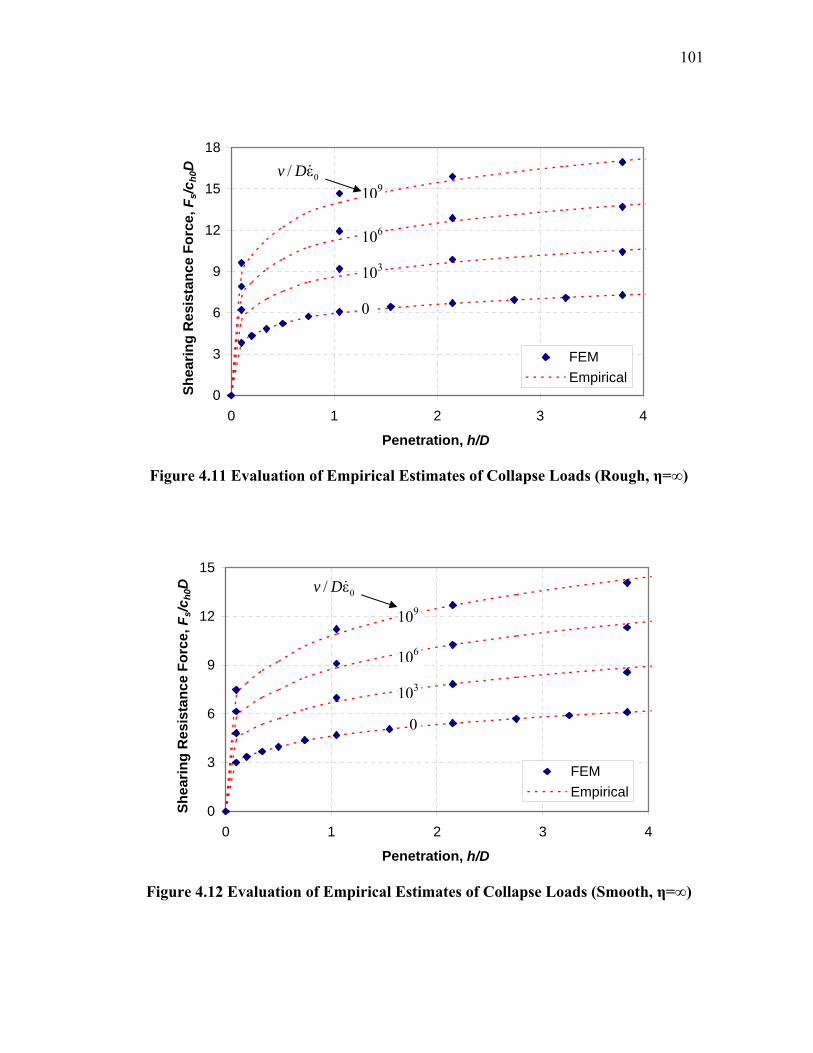
101

0

3

6

9

12

15

18

0 1 2 3 4

Penetration, h/D

Shea

ring

Res

ista

nce

Forc

e, F

s/ch0

D

FEMEmpirical

Figure 4.11 Evaluation of Empirical Estimates of Collapse Loads (Rough, η=∞)

0

3

6

9

12

15

0 1 2 3 4

Penetration, h/D

Shea

ring

Res

ista

nce

Forc

e, F

s/ch0

D

FEMEmpirical

Figure 4.12 Evaluation of Empirical Estimates of Collapse Loads (Smooth, η=∞)

0/ εv D 109

106

103

0

0/ εv D

109

106

103

0

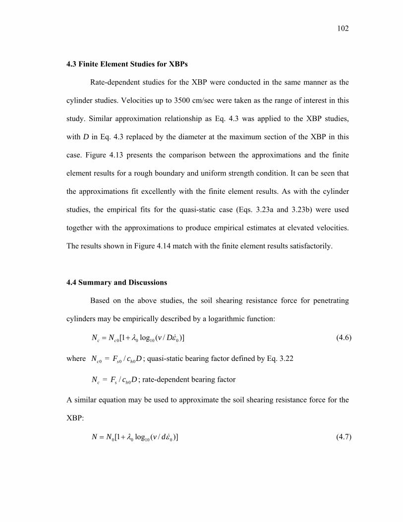
102

4.3 Finite Element Studies for XBPs

Rate-dependent studies for the XBP were conducted in the same manner as the

cylinder studies. Velocities up to 3500 cm/sec were taken as the range of interest in this

study. Similar approximation relationship as Eq. 4.3 was applied to the XBP studies,

with D in Eq. 4.3 replaced by the diameter at the maximum section of the XBP in this

case. Figure 4.13 presents the comparison between the approximations and the finite

element results for a rough boundary and uniform strength condition. It can be seen that

the approximations fit excellently with the finite element results. As with the cylinder

studies, the empirical fits for the quasi-static case (Eqs. 3.23a and 3.23b) were used

together with the approximations to produce empirical estimates at elevated velocities.

The results shown in Figure 4.14 match with the finite element results satisfactorily.

4.4 Summary and Discussions

Based on the above studies, the soil shearing resistance force for penetrating

cylinders may be empirically described by a logarithmic function:

0 0 10 0[1 log ( / )]c cN N v Dλ ε= + (4.6)

where 0cN = 0 0/s hF c D ; quasi-static bearing factor defined by Eq. 3.22

cN = 0/s hF c D ; rate-dependent bearing factor

A similar equation may be used to approximate the soil shearing resistance force for the

XBP:

0 0 10 0[1 log ( / )]N N v dλ ε= + (4.7)

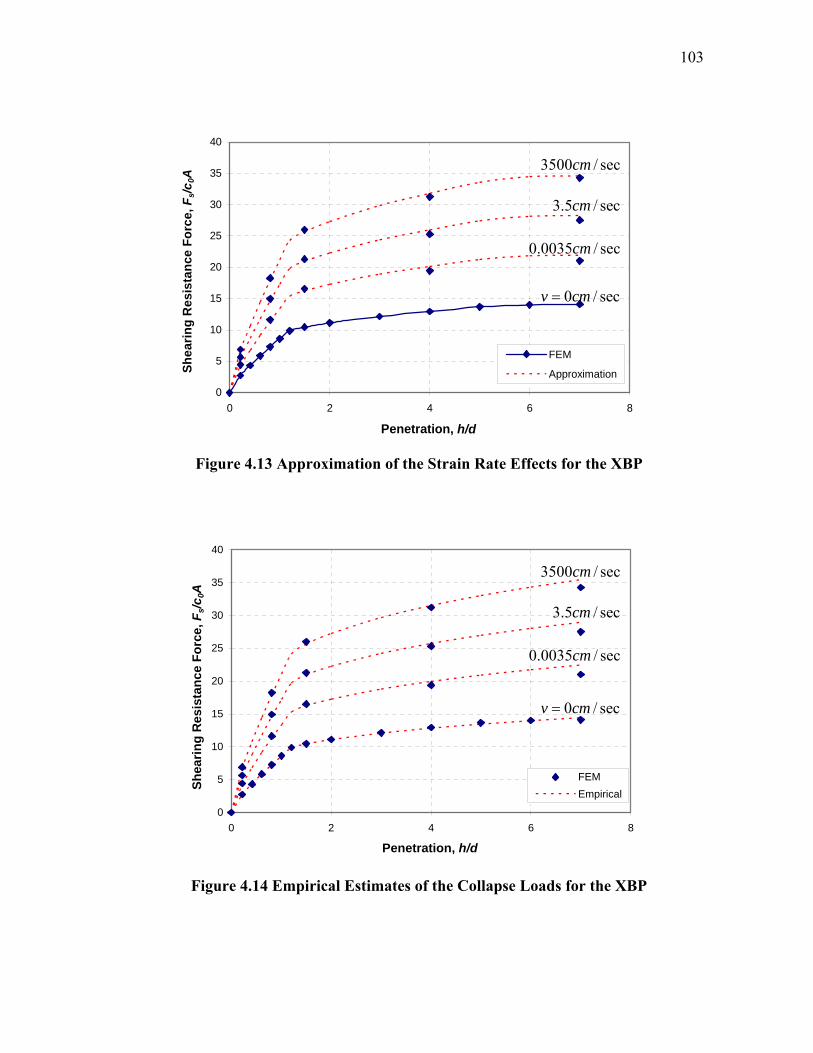
103

0

5

10

15

20

25

30

35

40

0 2 4 6 8

Penetration, h/d

Shea

ring

Res

ista

nce

Forc

e, F

s/c0A

FEM

Approximation

Figure 4.13 Approximation of the Strain Rate Effects for the XBP

0

5

10

15

20

25

30

35

40

0 2 4 6 8

Penetration, h/d

Shea

ring

Res

ista

nce

Forc

e, F

s/c0A

FEMEmpirical

Figure 4.14 Empirical Estimates of the Collapse Loads for the XBP

0 / secv cm=

3.5 / seccm

3500 / seccm

0 / secv cm=

0.0035 / seccm

3.5 / seccm

3500 / seccm

0.0035 / seccm

104

where 0N = 0 0/sF c A ; quasi-static bearing factor defined by Eqs. 3.23

N = 0/sF c A ; rate-dependent bearing factor

For rate-dependent studies, direct use of the plastic limit analysis methods can

not be made. A rate-dependent model can not include slip surfaces because strain rates

are effectively infinite. However, the rate-independent solutions are still useful as

reference cases.

In this analysis the inertial resistance of the soil is ignored because the range of

impact velocities of interest is very low. Care should be taken to investigate these effects

for significantly higher penetration rates.

105

CHAPTER V

PREDICTIVE MODELS

5.1 Penetration Studies

Based on the previously described studies and a rigid body projectile model, a

predictive model for the depth of penetration of cylinders has been developed. Model

predictions were compared to the results of the experimental penetration tests.

5.1.1 Penetration Model

If the penetrating cylinder is modeled as a rigid body, the forces acting on the

cylinder during penetration include the weight W, soil shearing resistance force Fs, and

the buoyancy force Fb (Figure 5.1). Thus, the acceleration of the cylinder can be defined

by the following equation (Aubeny and Dunlap, 2003):

/ 1 / /s ba g F W F W= − − (5.1)

where a = acceleration of the cylinder

g = gravitational acceleration

The buoyant force Fb comprises the soil buoyant force and the buoyant force of water (if

the cylinder is submerged). The buoyant force of water is simply the unit weight of

water multiplied by the volume of cylinder being submerged. It was not considered in

this analysis for the purpose of calibration with the penetration tests by Aubeny and

Dunlap (2003), but it can be easily added.

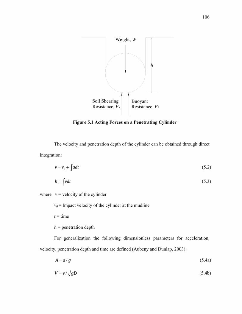
106

Figure 5.1 Acting Forces on a Penetrating Cylinder

The velocity and penetration depth of the cylinder can be obtained through direct

integration:

0v v adt= + ∫ (5.2)

h vdt= ∫ (5.3)

where v = velocity of the cylinder

v0 = Impact velocity of the cylinder at the mudline

t = time

h = penetration depth

For generalization the following dimensionless parameters for acceleration,

velocity, penetration depth and time are defined (Aubeny and Dunlap, 2003):

/A a g= (5.4a)

/V v gD= (5.4b)

Weight, W

Soil ShearingResistance, Fs

BuoyantResistance, Fb

h

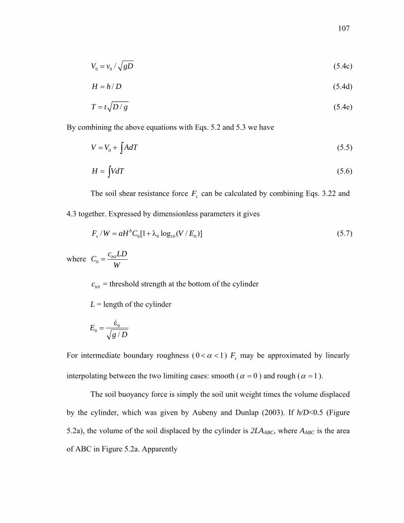
107

0 0 /V v gD= (5.4c)

/H h D= (5.4d)

/T t D g= (5.4e)

By combining the above equations with Eqs. 5.2 and 5.3 we have

0V V AdT= + ∫ (5.5)

H VdT= ∫ (5.6)

The soil shear resistance force sF can be calculated by combining Eqs. 3.22 and

4.3 together. Expressed by dimensionless parameters it gives

0 0 10 0/ [1 λ log ( / )]bsF W aH C V E= + (5.7)

where 00

hc LDCW

=

0hc = threshold strength at the bottom of the cylinder

L = length of the cylinder

00

ε/

Eg D

=

For intermediate boundary roughness ( 0 1α< < ) sF may be approximated by linearly

interpolating between the two limiting cases: smooth ( 0α = ) and rough ( 1α = ).

The soil buoyancy force is simply the soil unit weight times the volume displaced

by the cylinder, which was given by Aubeny and Dunlap (2003). If h/D<0.5 (Figure

5.2a), the volume of the soil displaced by the cylinder is 2LAABC, where AABC is the area

of ABC in Figure 5.2a. Apparently

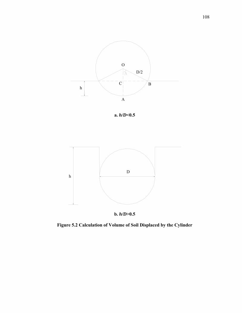
108

D/2

O

C B

A

h

a. h/D<0.5

hD

b. h/D>0.5

Figure 5.2 Calculation of Volume of Soil Displaced by the Cylinder

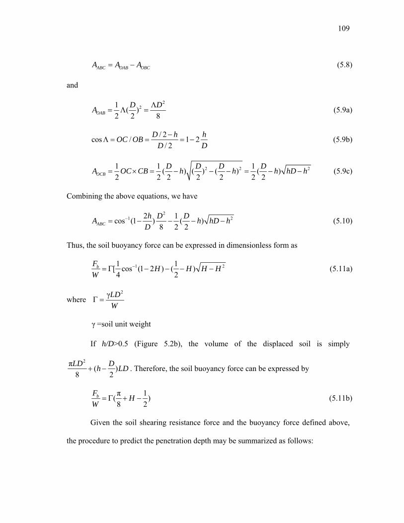
109

ABC OAB OBCA A A= − (5.8)

and

2

21 ( )2 2 8OAB

D DA Λ= Λ = (5.9a)

/ 2cos / 1 2/ 2

D h hOC OBD D

−Λ = = = − (5.9b)

2 2 21 1 1( ) ( ) ( ) ( )2 2 2 2 2 2 2OCB

D D D DA OC CB h h h hD h= × = − − − = − − (5.9c)

Combining the above equations, we have

2

1 22 1cos (1 ) ( )8 2 2ABC

h D DA h hD hD

−= − − − − (5.10)

Thus, the soil buoyancy force can be expressed in dimensionless form as

1 21 1[ cos (1 2 ) ( )4 2

bF H H H HW

−= Γ − − − − (5.11a)

where 2γLD

WΓ =

γ =soil unit weight

If h/D>0.5 (Figure 5.2b), the volume of the displaced soil is simply

2π ( )8 2

LD Dh LD+ − . Therefore, the soil buoyancy force can be expressed by

π 1( )8 2

bF HW

= Γ + − (5.11b)

Given the soil shearing resistance force and the buoyancy force defined above,

the procedure to predict the penetration depth may be summarized as follows:

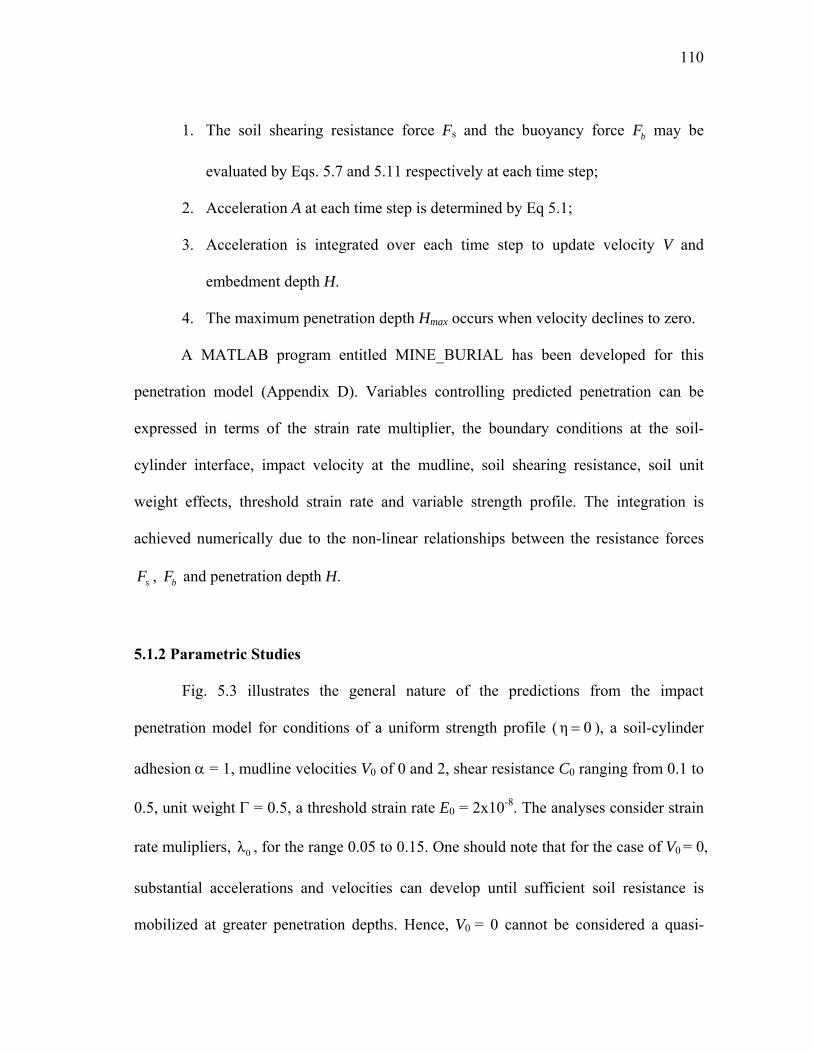
110

1. The soil shearing resistance force Fs and the buoyancy force bF may be

evaluated by Eqs. 5.7 and 5.11 respectively at each time step;

2. Acceleration A at each time step is determined by Eq 5.1;

3. Acceleration is integrated over each time step to update velocity V and

embedment depth H.

4. The maximum penetration depth Hmax occurs when velocity declines to zero.

A MATLAB program entitled MINE_BURIAL has been developed for this

penetration model (Appendix D). Variables controlling predicted penetration can be

expressed in terms of the strain rate multiplier, the boundary conditions at the soil-

cylinder interface, impact velocity at the mudline, soil shearing resistance, soil unit

weight effects, threshold strain rate and variable strength profile. The integration is

achieved numerically due to the non-linear relationships between the resistance forces

sF , bF and penetration depth H.

5.1.2 Parametric Studies

Fig. 5.3 illustrates the general nature of the predictions from the impact

penetration model for conditions of a uniform strength profile (η 0= ), a soil-cylinder

adhesion α = 1, mudline velocities V0 of 0 and 2, shear resistance C0 ranging from 0.1 to

0.5, unit weight Γ = 0.5, a threshold strain rate E0 = 2x10-8. The analyses consider strain

rate mulipliers, 0λ , for the range 0.05 to 0.15. One should note that for the case of V0 = 0,

substantial accelerations and velocities can develop until sufficient soil resistance is

mobilized at greater penetration depths. Hence, V0 = 0 cannot be considered a quasi-

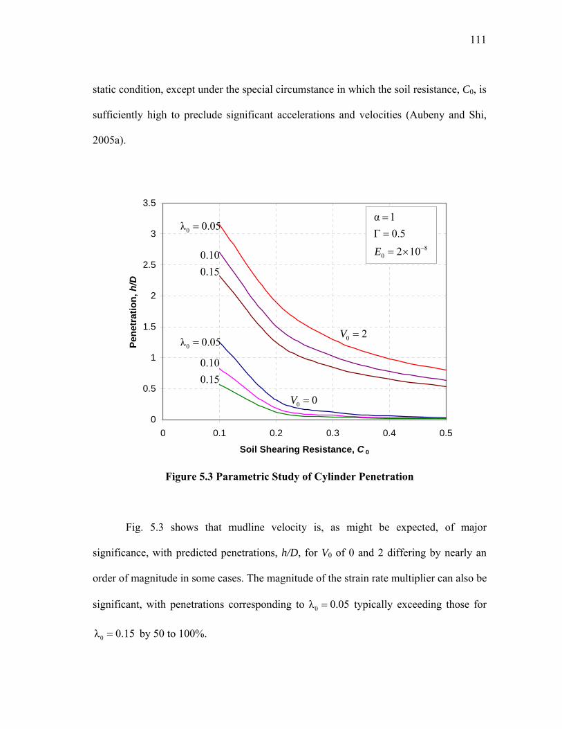
111

static condition, except under the special circumstance in which the soil resistance, C0, is

sufficiently high to preclude significant accelerations and velocities (Aubeny and Shi,

2005a).

0

0.5

1

1.5

2

2.5

3

3.5

0 0.1 0.2 0.3 0.4 0.5

Soil Shearing Resistance, C 0

Pene

trat

ion,

h/D

Figure 5.3 Parametric Study of Cylinder Penetration

Fig. 5.3 shows that mudline velocity is, as might be expected, of major

significance, with predicted penetrations, h/D, for V0 of 0 and 2 differing by nearly an

order of magnitude in some cases. The magnitude of the strain rate multiplier can also be

significant, with penetrations corresponding to 0λ 0.05= typically exceeding those for

0λ 0.15= by 50 to 100%.

0λ 0.05=

0.10 0.15

0λ 0.05=

0.10 0.15

80

α 10.52 10E −

=Γ =

= ×

0 2V =

0 0V =

112

5.1.3 Rate-Dependent Strength and Sensitivity

Due to the very soft soils under consideration, conventional laboratory tests

involving uniform distributions of strains and strain rates were not feasible. In such

circumstances, recourse must be taken to intrusive methods for strength measurements

involving highly non-uniform distributions of strain and strain rates for which any

assessment of strain rate effects entails considerable uncertainty. In the case of this study

the MV shear apparatus was used to estimate soil strength, but a similar observation

would apply to alternative intrusive test methods such as the cone penetrometer or the T-

bar.

An assessment of the dependence of shear strength on strain rate is possible by

varying the rate of rotation,θ , in the MV shear test. Fig. 5.4 illustrates the results of this

procedure for the reconstituted marine soils under consideration in this study. While the

MV shear strength versus rotation rate relationship in Fig. 5.4 is relatively simple,

applying the data to the impact penetration model actually requires a number of

assumptions, some of which have limited theoretical or experimental support at present.

For the present study we assume that the MV shear strength fits a framework analogous

to that defined by Eqs. 4.2; i.e., it may be expressed in terms of rotation rate as follows

(Aubeny and Shi, 2005a):

( )0 0 10 01 λ log θ / θmv mv mvc c ⎡ ⎤= +⎣ ⎦ (5.12)

113

0

0.5

1

1.5

2

0.0001 0.001 0.01 0.1 1Min

iatu

re V

ane

Stre

ngth

, cm

v (kPa

)

Rotation Rate, θ (rad/sec).

Best fit:c

mv = 1.87+0.138 log

10(θ).

Figure 5.4 Strain Rate Dependence from MV Test (Aubeny and Shi, 2005a)

where cmv is the shear strength associated with rotation rate θ , cmv0 is the threshold shear

strength associated with the threshold rotation rate 0θ , and 0λmv is the strain rate

multiplier for the MV test.

We also assume that the MV strain rate multiplier 0λmv approximates the strain

rate multiplier for collapse loading of a horizontal cylinder and 0ρ . Furthermore, we

assume that the threshold rotation rate 0θ can be taken as the threshold strain rate 0ε

(Aubeny and Shi, 2005a).

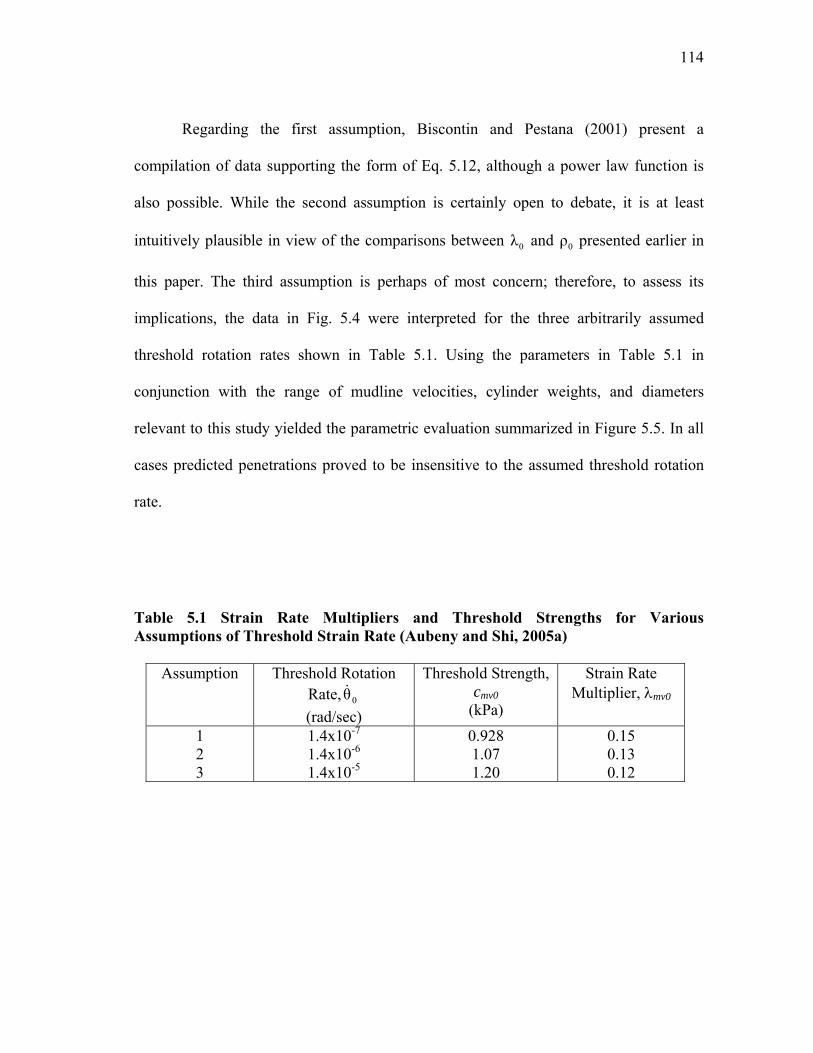
114

Regarding the first assumption, Biscontin and Pestana (2001) present a

compilation of data supporting the form of Eq. 5.12, although a power law function is

also possible. While the second assumption is certainly open to debate, it is at least

intuitively plausible in view of the comparisons between 0λ and 0ρ presented earlier in

this paper. The third assumption is perhaps of most concern; therefore, to assess its

implications, the data in Fig. 5.4 were interpreted for the three arbitrarily assumed

threshold rotation rates shown in Table 5.1. Using the parameters in Table 5.1 in

conjunction with the range of mudline velocities, cylinder weights, and diameters

relevant to this study yielded the parametric evaluation summarized in Figure 5.5. In all

cases predicted penetrations proved to be insensitive to the assumed threshold rotation

rate.

Table 5.1 Strain Rate Multipliers and Threshold Strengths for Various Assumptions of Threshold Strain Rate (Aubeny and Shi, 2005a)

Assumption Threshold Rotation Rate, 0θ (rad/sec)

Threshold Strength, cmv0

(kPa)

Strain Rate Multiplier, λmv0

1 2 3

1.4x10-7

1.4x10-6

1.4x10-5

0.928 1.07 1.20

0.15 0.13 0.12

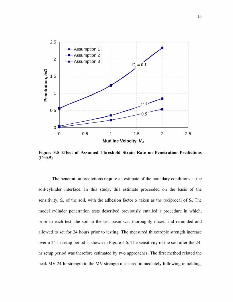
115

0

0.5

1

1.5

2

2.5

0 0.5 1 1.5 2 2.5

Mudline Velocity, V 0

Pene

trat

ion,

h/D

Assumption 1Assumption 2Assumption 3

Figure 5.5 Effect of Assumed Threshold Strain Rate on Penetration Predictions (Г=0.5)

The penetration predictions require an estimate of the boundary conditions at the

soil-cylinder interface. In this study, this estimate proceeded on the basis of the

sensitivity, St, of the soil, with the adhesion factor α taken as the reciprocal of St. The

model cylinder penetration tests described previously entailed a procedure in which,

prior to each test, the soil in the test basin was thoroughly mixed and remolded and

allowed to set for 24 hours prior to testing. The measured thixotropic strength increase

over a 24-hr setup period is shown in Figure 5.6. The sensitivity of the soil after the 24-

hr setup period was therefore estimated by two approaches. The first method related the

peak MV 24-hr strength to the MV strength measured immediately following remolding.

0 0.1C =

0.3

0.5

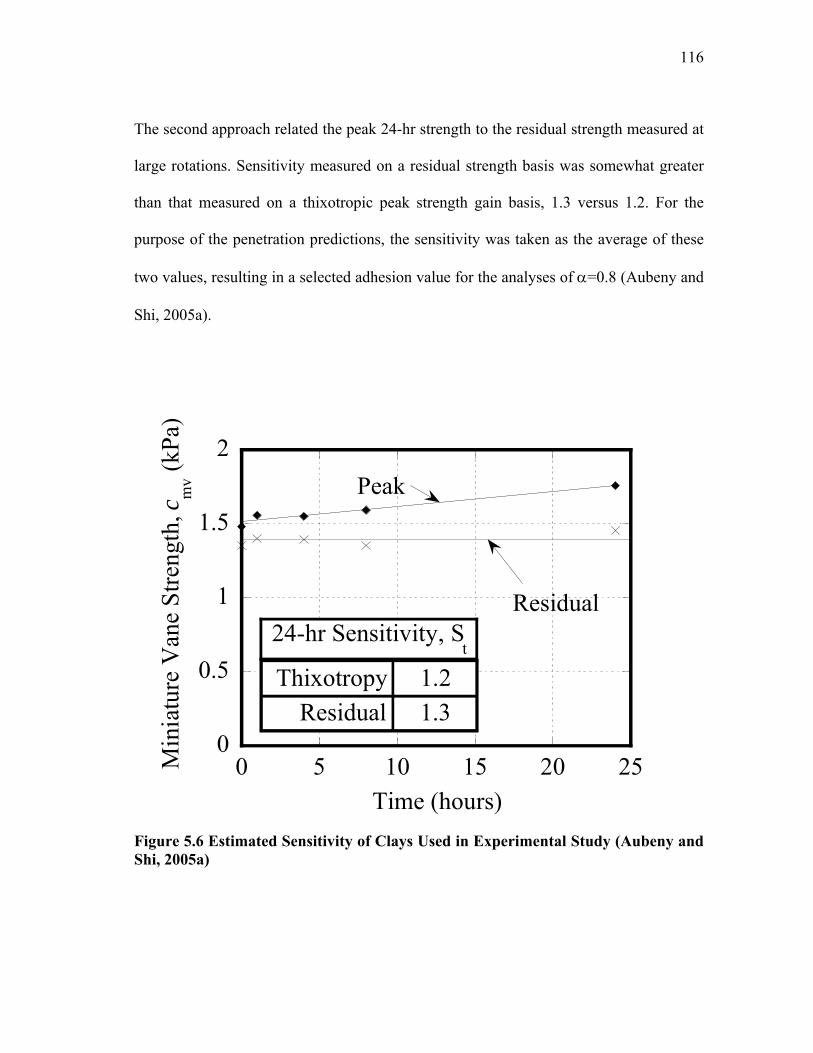
116

The second approach related the peak 24-hr strength to the residual strength measured at

large rotations. Sensitivity measured on a residual strength basis was somewhat greater

than that measured on a thixotropic peak strength gain basis, 1.3 versus 1.2. For the

purpose of the penetration predictions, the sensitivity was taken as the average of these

two values, resulting in a selected adhesion value for the analyses of α=0.8 (Aubeny and

Shi, 2005a).

0

0.5

1

1.5

2

0 5 10 15 20 25Min

iatu

re V

ane

Stre

ngth

, cm

v (kPa

)

Time (hours)

Peak

Residual

1.2 Thixotropy1.3Residual

24-hr Sensitivity, St

Figure 5.6 Estimated Sensitivity of Clays Used in Experimental Study (Aubeny and Shi, 2005a)

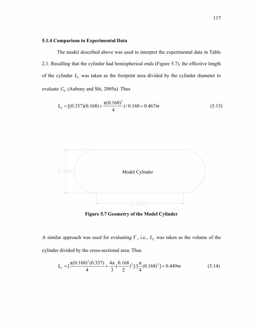
117

5.1.4 Comparison to Experimental Data

The model described above was used to interpret the experimental data in Table

2.1. Recalling that the cylinder had hemispherical ends (Figure 5.7), the effective length

of the cylinder CL was taken as the footprint area divided by the cylinder diameter to

evaluate 0C (Aubeny and Shi, 2005a). Thus

2π(0.168)[(0.337)(0.168) ) / 0.168 0.467

4CL m= + = (5.13)

Model Cylinder

Figure 5.7 Geometry of the Model Cylinder

A similar approach was used for evaluating Γ , i.e., CL was taken as the volume of the

cylinder divided by the cross-sectional area. Thus

2

3 2π(0.168) (0.337) 4π 0.168 π[ ( ) ] /[ (0.168) ] 0.4494 3 2 4CL m= + = (5.14)

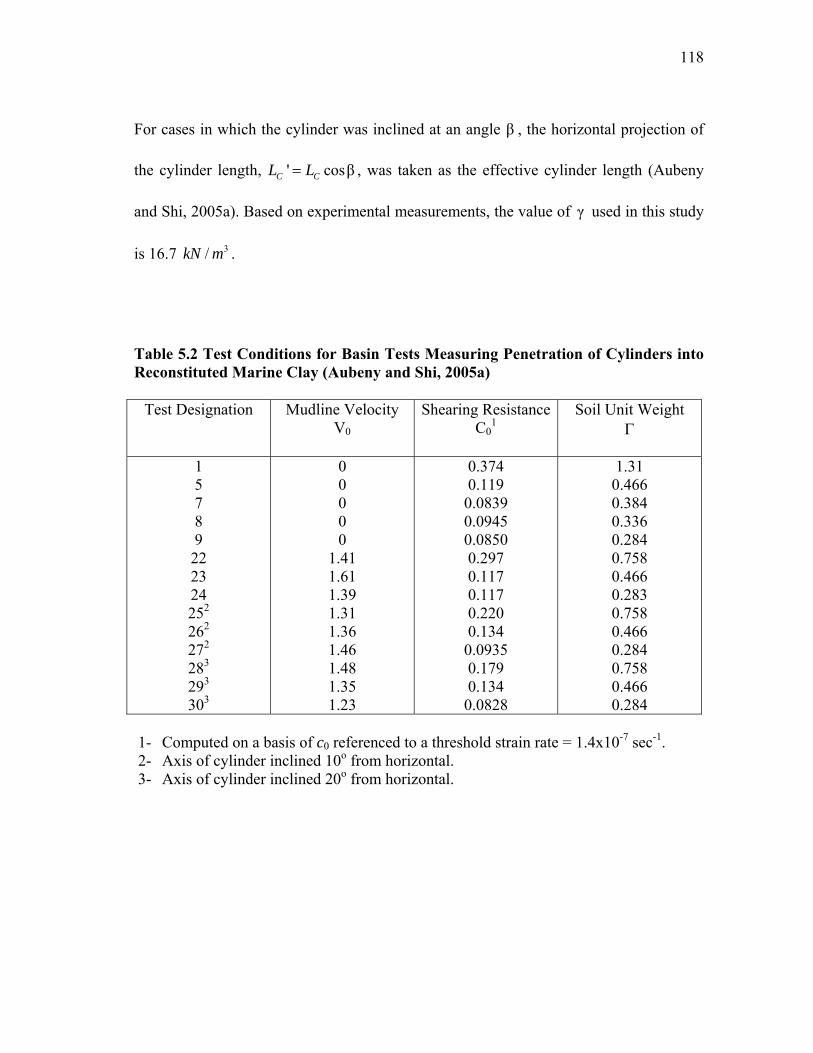
118

For cases in which the cylinder was inclined at an angle β , the horizontal projection of

the cylinder length, ' cosβC CL L= , was taken as the effective cylinder length (Aubeny

and Shi, 2005a). Based on experimental measurements, the value of γ used in this study

is 16.7 3/kN m .

Table 5.2 Test Conditions for Basin Tests Measuring Penetration of Cylinders into Reconstituted Marine Clay (Aubeny and Shi, 2005a)

Test Designation Mudline Velocity V0

Shearing ResistanceC0

1 Soil Unit Weight

Γ

1 5 7 8 9 22 23 24 252 262 272 283 293 303

0 0 0 0 0

1.41 1.61 1.39 1.31 1.36 1.46 1.48 1.35 1.23

0.374 0.119 0.0839 0.0945 0.0850 0.297 0.117 0.117 0.220 0.134 0.0935 0.179 0.134 0.0828

1.31 0.466 0.384 0.336 0.284 0.758 0.466 0.283 0.758 0.466 0.284 0.758 0.466 0.284

1- Computed on a basis of c0 referenced to a threshold strain rate = 1.4x10-7 sec-1. 2- Axis of cylinder inclined 10o from horizontal. 3- Axis of cylinder inclined 20o from horizontal.

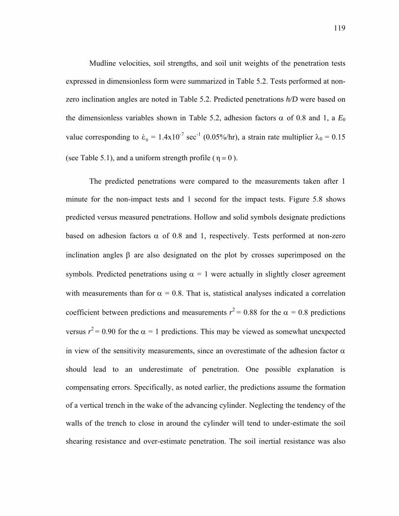
119

Mudline velocities, soil strengths, and soil unit weights of the penetration tests

expressed in dimensionless form were summarized in Table 5.2. Tests performed at non-

zero inclination angles are noted in Table 5.2. Predicted penetrations h/D were based on

the dimensionless variables shown in Table 5.2, adhesion factors α of 0.8 and 1, a E0

value corresponding to 0ε = 1.4x10-7 sec-1 (0.05%/hr), a strain rate multiplier λ0 = 0.15

(see Table 5.1), and a uniform strength profile (η 0= ).

The predicted penetrations were compared to the measurements taken after 1

minute for the non-impact tests and 1 second for the impact tests. Figure 5.8 shows

predicted versus measured penetrations. Hollow and solid symbols designate predictions

based on adhesion factors α of 0.8 and 1, respectively. Tests performed at non-zero

inclination angles β are also designated on the plot by crosses superimposed on the

symbols. Predicted penetrations using α = 1 were actually in slightly closer agreement

with measurements than for α = 0.8. That is, statistical analyses indicated a correlation

coefficient between predictions and measurements r2 = 0.88 for the α = 0.8 predictions

versus r2 = 0.90 for the α = 1 predictions. This may be viewed as somewhat unexpected

in view of the sensitivity measurements, since an overestimate of the adhesion factor α

should lead to an underestimate of penetration. One possible explanation is

compensating errors. Specifically, as noted earlier, the predictions assume the formation

of a vertical trench in the wake of the advancing cylinder. Neglecting the tendency of the

walls of the trench to close in around the cylinder will tend to under-estimate the soil

shearing resistance and over-estimate penetration. The soil inertial resistance was also

120

neglected in this analysis. In addition, the soil shear resistance force is estimated from

plane solutions; hence, end resistance effects are neglected. An over-estimate of the

adhesion factor, α = 1, may actually compensate for these effects, resulting in somewhat

better predictions (Aubeny and Shi, 2005a).

The overall level of agreement between predicted and measured penetrations for

the tests performed at inclinations β of 10 and 20 degrees is comparable to that for the

horizontal tests, suggesting that predictions based on a horizontally oriented cylinder can

provide reasonable penetration estimates for shallow inclination angles. Overall, given

the level of uncertainty in characterizing the strength properties of the soil, the predicted

penetrations agree reasonably well with measurements.

Figure 5.9 presents the predictions of penetrations without strain rate correction

( λ 0= ) for the α 1= case. We can see that the predictions distinctly over-estimate the

penetrations when the effect of strength increase with strain rate is neglected, and the

value of the statistical correlation coefficient 2r is only 0.64. By comparison of Figure

5.8 and Figure 5.9 we may conclude that the mechanism of strain rate correction

incorporated in this penetration model is effective.

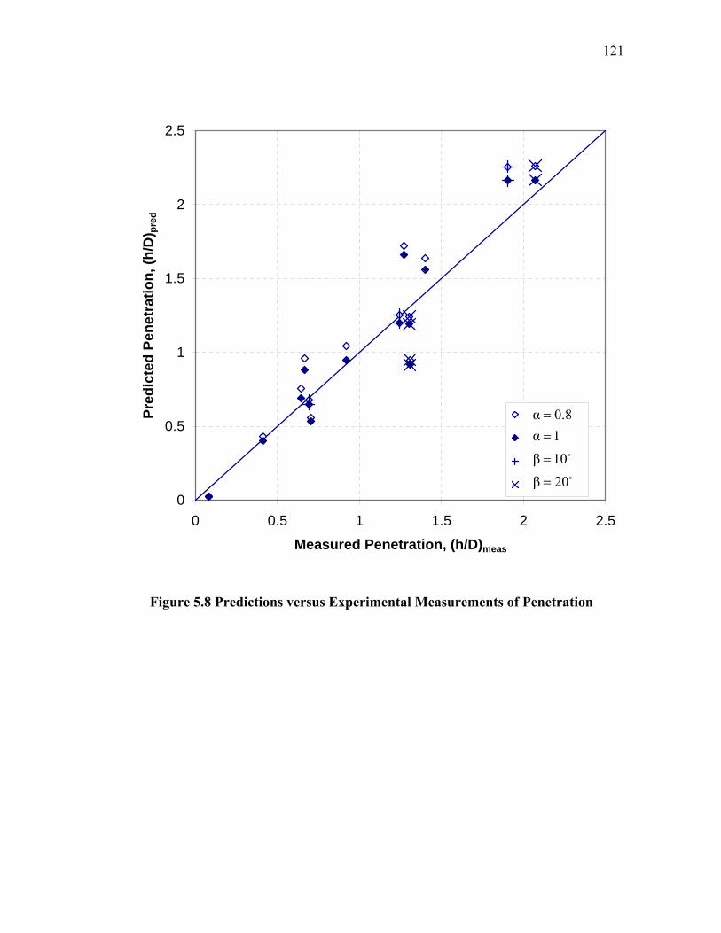
121

0

0.5

1

1.5

2

2.5

0 0.5 1 1.5 2 2.5

Measured Penetration, (h/D)meas

Pred

icte

d Pe

netr

atio

n, (h

/D) p

red

Figure 5.8 Predictions versus Experimental Measurements of Penetration

α 0.8α 1β 10β 20

==

=

=

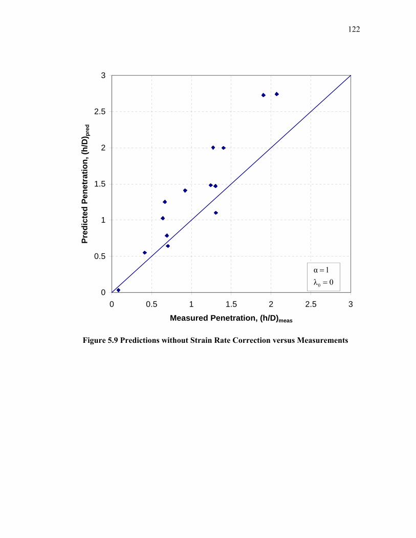
122

0

0.5

1

1.5

2

2.5

3

0 0.5 1 1.5 2 2.5 3

Measured Penetration, (h/D)meas

Pred

icte

d Pe

netr

atio

n, (h

/D) p

red

Figure 5.9 Predictions without Strain Rate Correction versus Measurements

0

α 1λ 0

==

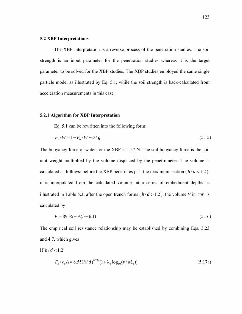
123

5.2 XBP Interpretations

The XBP interpretation is a reverse process of the penetration studies. The soil

strength is an input parameter for the penetration studies whereas it is the target

parameter to be solved for the XBP studies. The XBP studies employed the same single

particle model as illustrated by Eq. 5.1, while the soil strength is back-calculated from

acceleration measurements in this case.

5.2.1 Algorithm for XBP Interpretation

Eq. 5.1 can be rewritten into the following form:

/ 1 / /s bF W F W a g= − − (5.15)

The buoyancy force of water for the XBP is 1.57 N. The soil buoyancy force is the soil

unit weight multiplied by the volume displaced by the penetrometer. The volume is

calculated as follows: before the XBP penetrates past the maximum section ( / 1.2h d < ),

it is interpolated from the calculated volumes at a series of embedment depths as

illustrated in Table 5.3; after the open trench forms ( / 1.2h d > ), the volume V in 3cm is

calculated by

89.35 ( 6.1)V A h= + − (5.16)

The empirical soil resistance relationship may be established by combining Eqs. 3.23

and 4.7, which gives

If / 1.2h d <

0.7560 0 10 0/ 8.55( / ) [1 λ log ( / ε )]sF c A h d v d= + (5.17a)

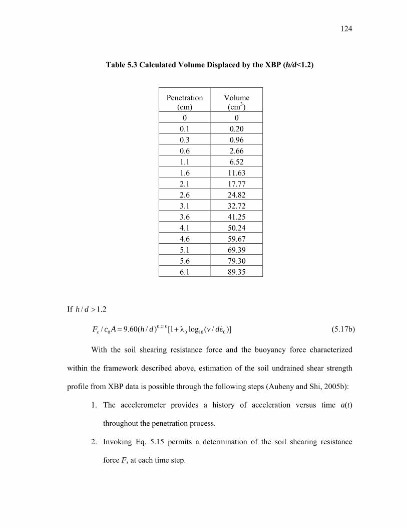
124

Table 5.3 Calculated Volume Displaced by the XBP (h/d<1.2)

Penetration (cm)

Volume (cm3)

0 0 0.1 0.20 0.3 0.96 0.6 2.66 1.1 6.52 1.6 11.63 2.1 17.77 2.6 24.82 3.1 32.72 3.6 41.25 4.1 50.24 4.6 59.67 5.1 69.39 5.6 79.30 6.1 89.35

If / 1.2h d >

0.2100 0 10 0/ 9.60( / ) [1 λ log ( / ε )]sF c A h d v d= + (5.17b)

With the soil shearing resistance force and the buoyancy force characterized

within the framework described above, estimation of the soil undrained shear strength

profile from XBP data is possible through the following steps (Aubeny and Shi, 2005b):

1. The accelerometer provides a history of acceleration versus time a(t)

throughout the penetration process.

2. Invoking Eq. 5.15 permits a determination of the soil shearing resistance

force Fs at each time step.

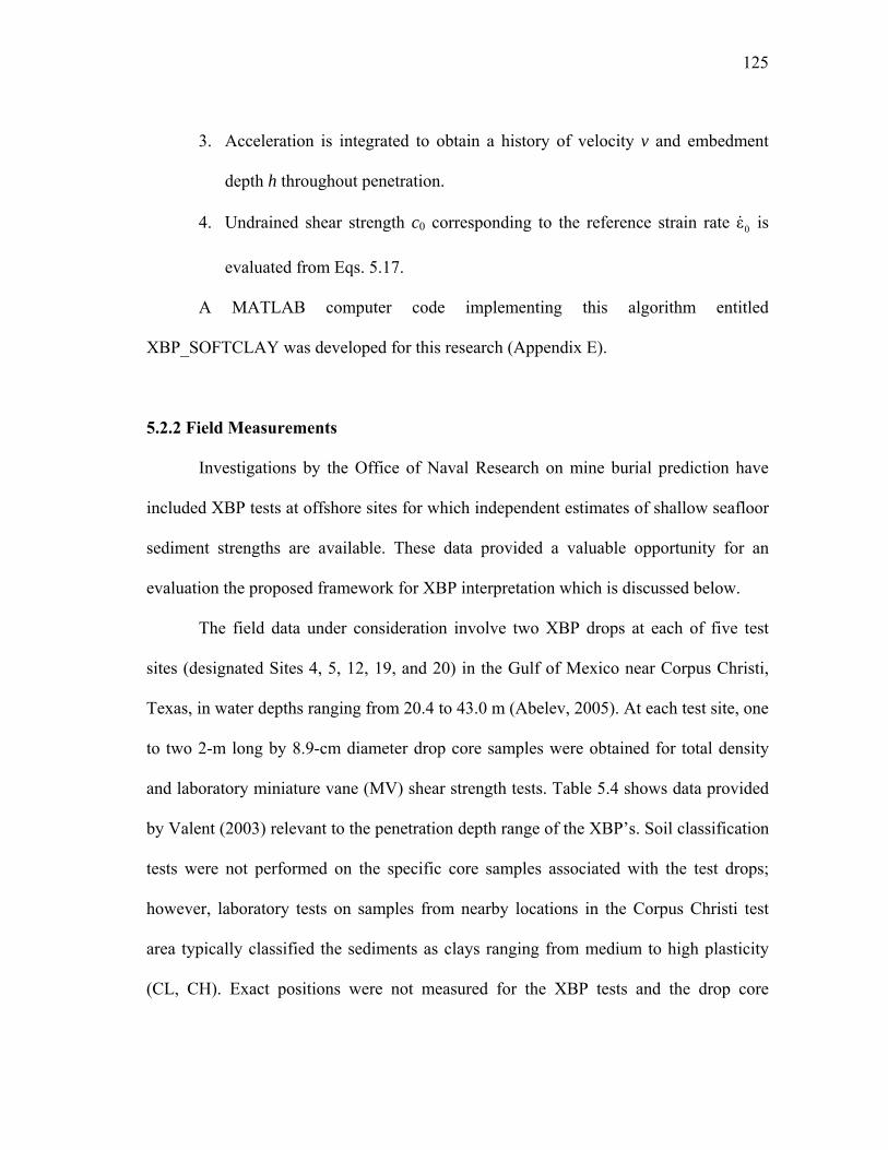
125

3. Acceleration is integrated to obtain a history of velocity v and embedment

depth h throughout penetration.

4. Undrained shear strength c0 corresponding to the reference strain rate 0ε is

evaluated from Eqs. 5.17.

A MATLAB computer code implementing this algorithm entitled

XBP_SOFTCLAY was developed for this research (Appendix E).

5.2.2 Field Measurements

Investigations by the Office of Naval Research on mine burial prediction have

included XBP tests at offshore sites for which independent estimates of shallow seafloor

sediment strengths are available. These data provided a valuable opportunity for an

evaluation the proposed framework for XBP interpretation which is discussed below.

The field data under consideration involve two XBP drops at each of five test

sites (designated Sites 4, 5, 12, 19, and 20) in the Gulf of Mexico near Corpus Christi,

Texas, in water depths ranging from 20.4 to 43.0 m (Abelev, 2005). At each test site, one

to two 2-m long by 8.9-cm diameter drop core samples were obtained for total density

and laboratory miniature vane (MV) shear strength tests. Table 5.4 shows data provided

by Valent (2003) relevant to the penetration depth range of the XBP’s. Soil classification

tests were not performed on the specific core samples associated with the test drops;

however, laboratory tests on samples from nearby locations in the Corpus Christi test

area typically classified the sediments as clays ranging from medium to high plasticity

(CL, CH). Exact positions were not measured for the XBP tests and the drop core

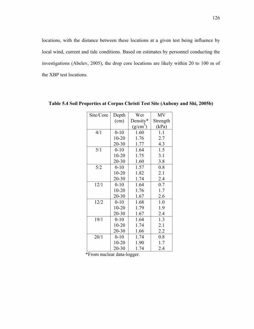
126

locations, with the distance between these locations at a given test being influence by

local wind, current and tide conditions. Based on estimates by personnel conducting the

investigations (Abelev, 2005), the drop core locations are likely within 20 to 100 m of

the XBP test locations.

Table 5.4 Soil Properties at Corpus Christi Test Site (Aubeny and Shi, 2005b)

Site/Core Depth

(cm) Wet

Density*(g/cm3)

MV Strength

(kPa) 4/1 0-10

10-20 20-30

1.60 1.76 1.77

1.1 2.7 4.3

5/1

0-10 10-20 20-30

1.64 1.75 1.60

1.5 3.1 3.8

5/2 0-10 10-20 20-30

1.57 1.82 1.74

0.8 2.1 2.4

12/1

0-10 10-20 20-30

1.64 1.76 1.67

0.7 1.7 2.6

12/2 0-10 10-20 20-30

1.68 1.79 1.67

1.0 1.9 2.4

19/1 0-10 10-20 20-30

1.64 1.74 1.66

1.3 2.1 2.2

20/1 0-10 10-20 20-30

1.74 1.90 1.74

0.8 1.7 2.4

*From nuclear data-logger.

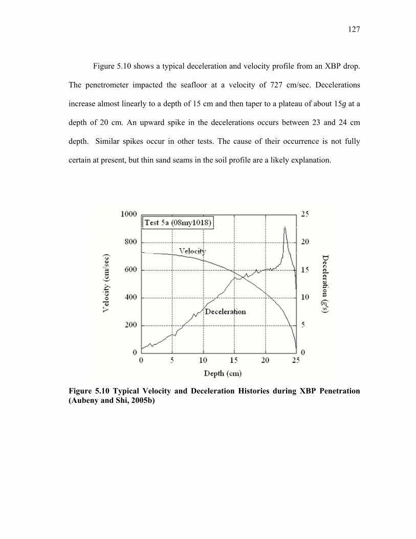
127

Figure 5.10 shows a typical deceleration and velocity profile from an XBP drop.

The penetrometer impacted the seafloor at a velocity of 727 cm/sec. Decelerations

increase almost linearly to a depth of 15 cm and then taper to a plateau of about 15g at a

depth of 20 cm. An upward spike in the decelerations occurs between 23 and 24 cm

depth. Similar spikes occur in other tests. The cause of their occurrence is not fully

certain at present, but thin sand seams in the soil profile are a likely explanation.

Figure 5.10 Typical Velocity and Deceleration Histories during XBP Penetration (Aubeny and Shi, 2005b)

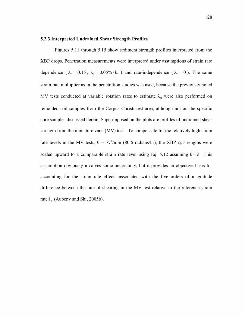
128

5.2.3 Interpreted Undrained Shear Strength Profiles

Figures 5.11 through 5.15 show sediment strength profiles interpreted from the

XBP drops. Penetration measurements were interpreted under assumptions of strain rate

dependence ( 0λ 0.15= , 0ε 0.05% / hr= ) and rate-independence ( 0λ 0= ). The same

strain rate multiplier as in the penetration studies was used, because the previously noted

MV tests conducted at variable rotation rates to estimate 0λ were also performed on

remolded soil samples from the Corpus Christi test area, although not on the specific

core samples discussed herein. Superimposed on the plots are profiles of undrained shear

strength from the miniature vane (MV) tests. To compensate for the relatively high strain

rate levels in the MV tests, θ = 77o/min (80.6 radians/hr), the XBP c0 strengths were

scaled upward to a comparable strain rate level using Eq. 5.12 assuming θ ε= . This

assumption obviously involves some uncertainty, but it provides an objective basis for

accounting for the strain rate effects associated with the five orders of magnitude

difference between the rate of shearing in the MV test relative to the reference strain

rate 0ε (Aubeny and Shi, 2005b).

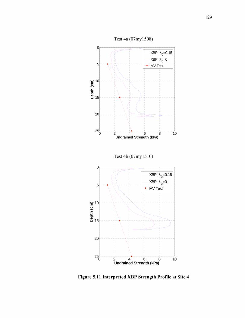
129

Test 4a (07my1508)

0 2 4 6 8 10

0

5

10

15

20

25

Dep

th (c

m)

Undrained Strength (kPa)

XBP, λ0=0.15

XBP, λ0=0

MV Test

Test 4b (07my1510)

0 2 4 6 8 10

0

5

10

15

20

25

Dep

th (c

m)

Undrained Strength (kPa)

XBP, λ0=0.15

XBP, λ0=0

MV Test

Figure 5.11 Interpreted XBP Strength Profile at Site 4

130

Test 5a (08my1018)

0 1 2 3 4 5 6 7

0

5

10

15

20

25

30

Dep

th (c

m)

Undrained Strength (kPa)

XBP, λ0=0.15

XBP, λ0=0

MV Test 1MV Test 2

Test 5b (08my1020)

0 1 2 3 4 5 6 7

0

5

10

15

20

25

30

Dep

th (c

m)

Undrained Strength (kPa)

XBP, λ0=0.15

XBP, λ0=0MV Test 1MV Test 2

Figure 5.12 Interpreted XBP Strength Profile at Site 5

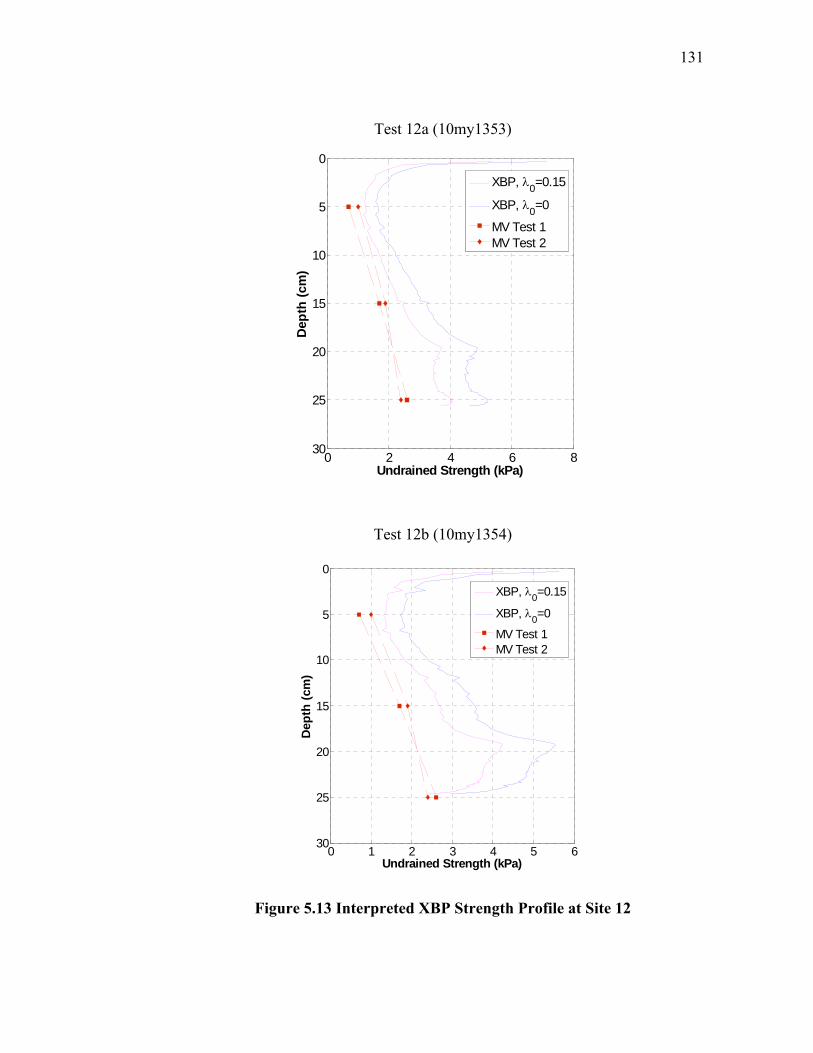
131

Test 12a (10my1353)

0 2 4 6 8

0

5

10

15

20

25

30

Dep

th (c

m)

Undrained Strength (kPa)

XBP, λ0=0.15

XBP, λ0=0

MV Test 1MV Test 2

Test 12b (10my1354)

0 1 2 3 4 5 6

0

5

10

15

20

25

30

Dep

th (c

m)

Undrained Strength (kPa)

XBP, λ0=0.15

XBP, λ0=0

MV Test 1MV Test 2

Figure 5.13 Interpreted XBP Strength Profile at Site 12

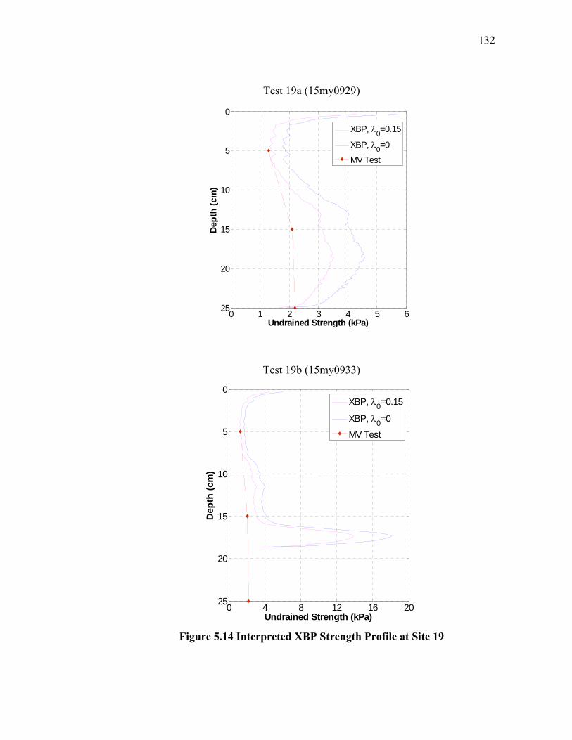
132

Test 19a (15my0929)

0 1 2 3 4 5 6

0

5

10

15

20

25

Dep

th (c

m)

Undrained Strength (kPa)

XBP, λ0=0.15

XBP, λ0=0

MV Test

Test 19b (15my0933)

0 4 8 12 16 20

0

5

10

15

20

25

Dep

th (c

m)

Undrained Strength (kPa)

XBP, λ0=0.15

XBP, λ0=0

MV Test

Figure 5.14 Interpreted XBP Strength Profile at Site 19

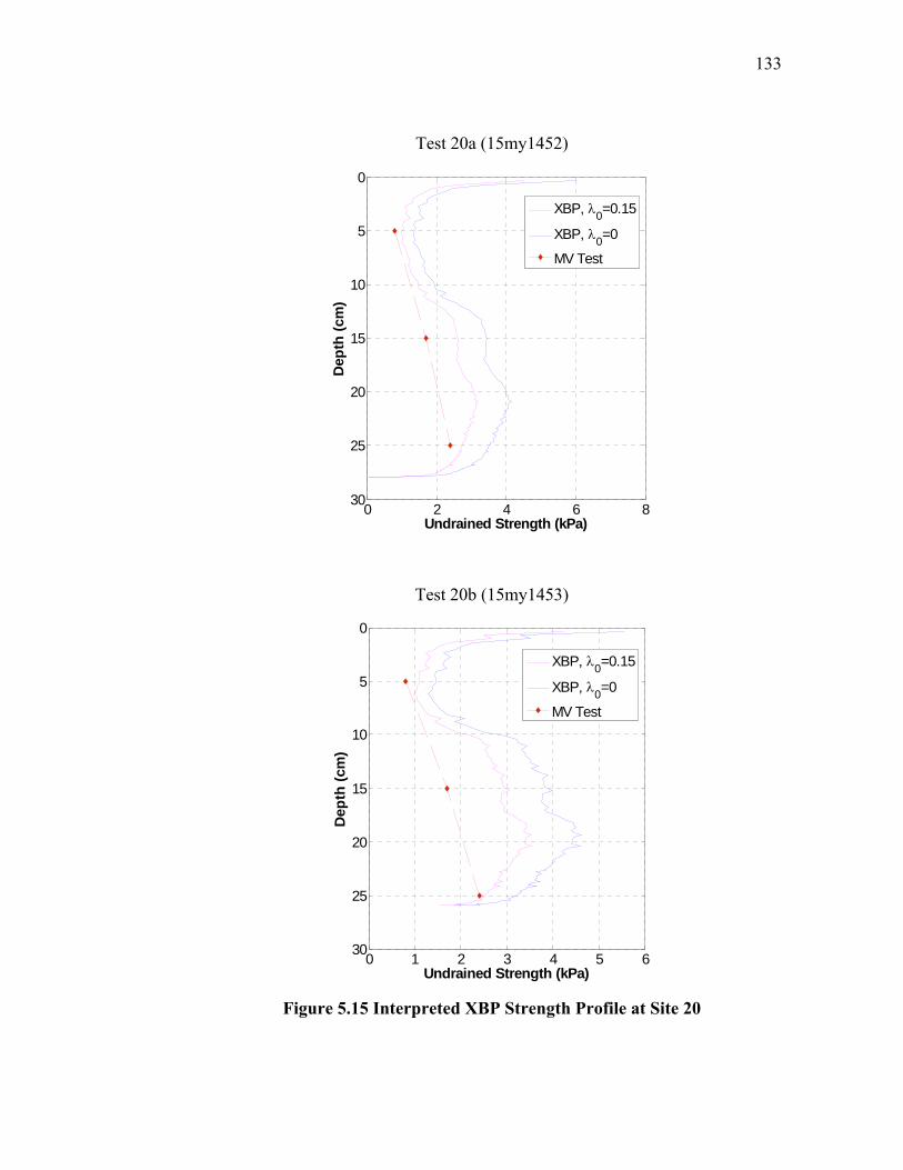
133

Test 20a (15my1452)

0 2 4 6 8

0

5

10

15

20

25

30

Dep

th (c

m)

Undrained Strength (kPa)

XBP, λ0=0.15

XBP, λ0=0

MV Test

Test 20b (15my1453)

0 1 2 3 4 5 6

0

5

10

15

20

25

30

Dep

th (c

m)

Undrained Strength (kPa)

XBP, λ0=0.15

XBP, λ0=0

MV Test

Figure 5.15 Interpreted XBP Strength Profile at Site 20

134

Examination of the interpreted XBP strength profiles vis-à-vis the MV strength

profiles reveals two regions where the XBP strengths are consistently unrealistic

(Aubeny and Shi, 2005b):

1. During the initial stages of penetration, the interpreted XBP strengths

severely over-estimate the reference MV strengths in all cases. A possible

source of this discrepancy is that this analysis does not account for the inertial

resistance from the soil and the hydrodynamic resistance from the water

column that may be significant during early stages of penetration. Neglecting

resistance from this source can lead to over-estimates of the sediment

shearing resistance. The depth of this initial phase of penetration for which

valid XBP strength interpretations are considered unreliable is taken as the

depth at which the apparent interpreted strength reaches a local minimum.

Figures 5.11 through 5.15 indicate unreliable strength estimates from the

XBP in the initial 5 cm ( / 1h d ≈ ) of penetration.

2. The apparent XBP strength precipitously declines in the final stages of

penetration. Elastic rebound of the soil as the penetration velocity declines to

zero, an effect not considered in Eq. 5.1, is a probable source of this

discrepancy.

Penetration measurements from intermediate depths between the initial and final

phases of penetration described above appear to provide a valid basis for estimating

sediment undrained shear strength. Comparisons between MV and interpreted XBP

strengths within this range of depths indicate the following (Aubeny and Shi, 2005b):

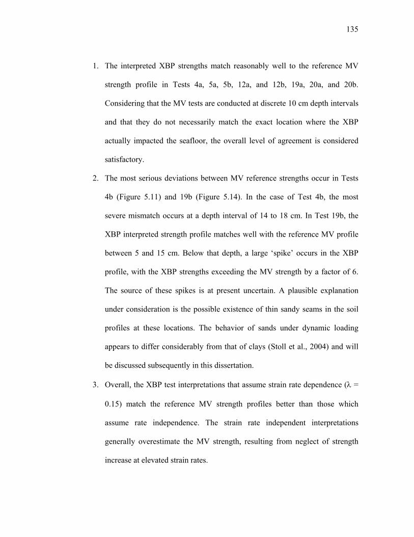
135

1. The interpreted XBP strengths match reasonably well to the reference MV

strength profile in Tests 4a, 5a, 5b, 12a, and 12b, 19a, 20a, and 20b.

Considering that the MV tests are conducted at discrete 10 cm depth intervals

and that they do not necessarily match the exact location where the XBP

actually impacted the seafloor, the overall level of agreement is considered

satisfactory.

2. The most serious deviations between MV reference strengths occur in Tests

4b (Figure 5.11) and 19b (Figure 5.14). In the case of Test 4b, the most

severe mismatch occurs at a depth interval of 14 to 18 cm. In Test 19b, the

XBP interpreted strength profile matches well with the reference MV profile

between 5 and 15 cm. Below that depth, a large ‘spike’ occurs in the XBP

profile, with the XBP strengths exceeding the MV strength by a factor of 6.

The source of these spikes is at present uncertain. A plausible explanation

under consideration is the possible existence of thin sandy seams in the soil

profiles at these locations. The behavior of sands under dynamic loading

appears to differ considerably from that of clays (Stoll et al., 2004) and will

be discussed subsequently in this dissertation.

3. Overall, the XBP test interpretations that assume strain rate dependence (λ =

0.15) match the reference MV strength profiles better than those which

assume rate independence. The strain rate independent interpretations

generally overestimate the MV strength, resulting from neglect of strength

increase at elevated strain rates.

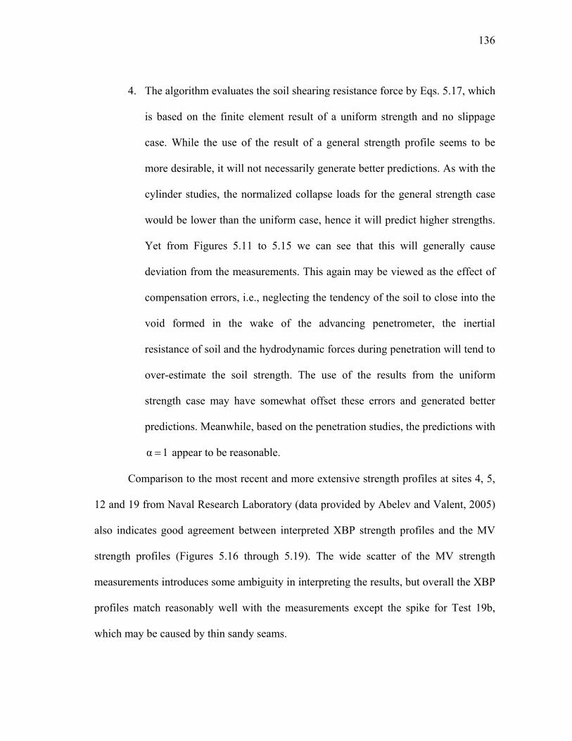
136

4. The algorithm evaluates the soil shearing resistance force by Eqs. 5.17, which

is based on the finite element result of a uniform strength and no slippage

case. While the use of the result of a general strength profile seems to be

more desirable, it will not necessarily generate better predictions. As with the

cylinder studies, the normalized collapse loads for the general strength case

would be lower than the uniform case, hence it will predict higher strengths.

Yet from Figures 5.11 to 5.15 we can see that this will generally cause

deviation from the measurements. This again may be viewed as the effect of

compensation errors, i.e., neglecting the tendency of the soil to close into the

void formed in the wake of the advancing penetrometer, the inertial

resistance of soil and the hydrodynamic forces during penetration will tend to

over-estimate the soil strength. The use of the results from the uniform

strength case may have somewhat offset these errors and generated better

predictions. Meanwhile, based on the penetration studies, the predictions with

α 1= appear to be reasonable.

Comparison to the most recent and more extensive strength profiles at sites 4, 5,

12 and 19 from Naval Research Laboratory (data provided by Abelev and Valent, 2005)

also indicates good agreement between interpreted XBP strength profiles and the MV

strength profiles (Figures 5.16 through 5.19). The wide scatter of the MV strength

measurements introduces some ambiguity in interpreting the results, but overall the XBP

profiles match reasonably well with the measurements except the spike for Test 19b,

which may be caused by thin sandy seams.

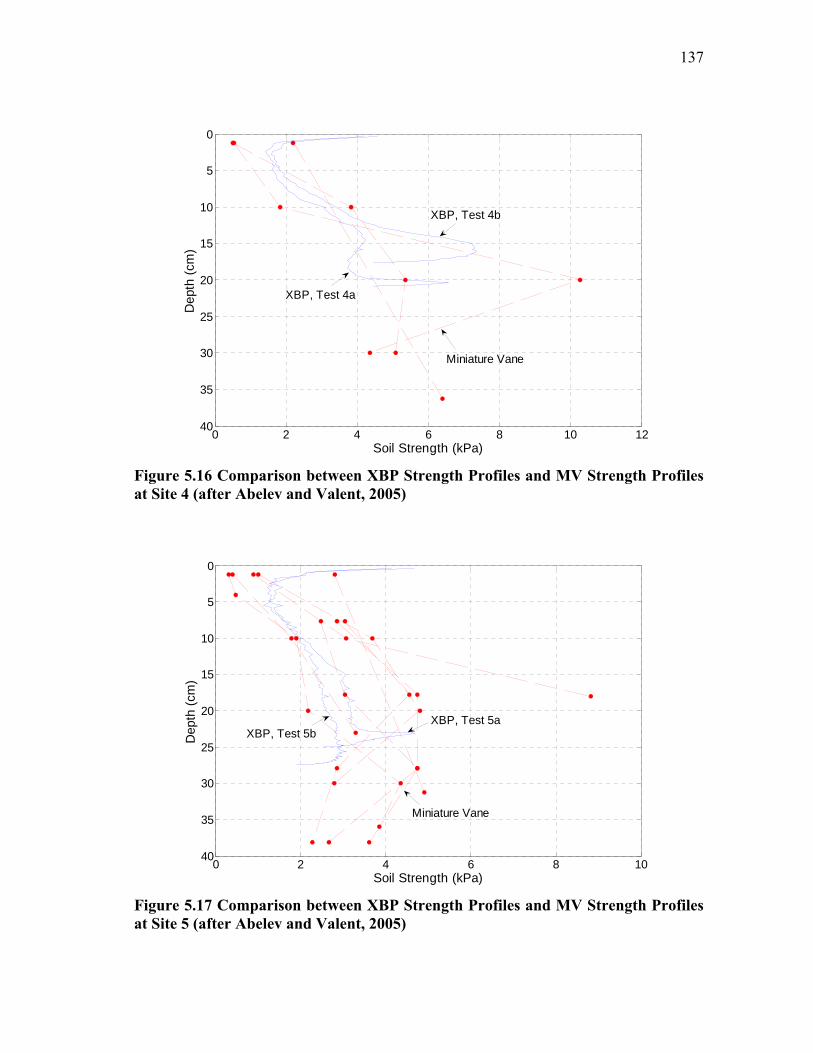
137

0 2 4 6 8 10 12

0

5

10

15

20

25

30

35

40

Dep

th (c

m)

Soil Strength (kPa)

XBP, Test 4a

XBP, Test 4b

Miniature Vane

Figure 5.16 Comparison between XBP Strength Profiles and MV Strength Profiles at Site 4 (after Abelev and Valent, 2005)

0 2 4 6 8 10

0

5

10

15

20

25

30

35

40

Dep

th (c

m)

Soil Strength (kPa)

XBP, Test 5aXBP, Test 5b

Miniature Vane

Figure 5.17 Comparison between XBP Strength Profiles and MV Strength Profiles at Site 5 (after Abelev and Valent, 2005)

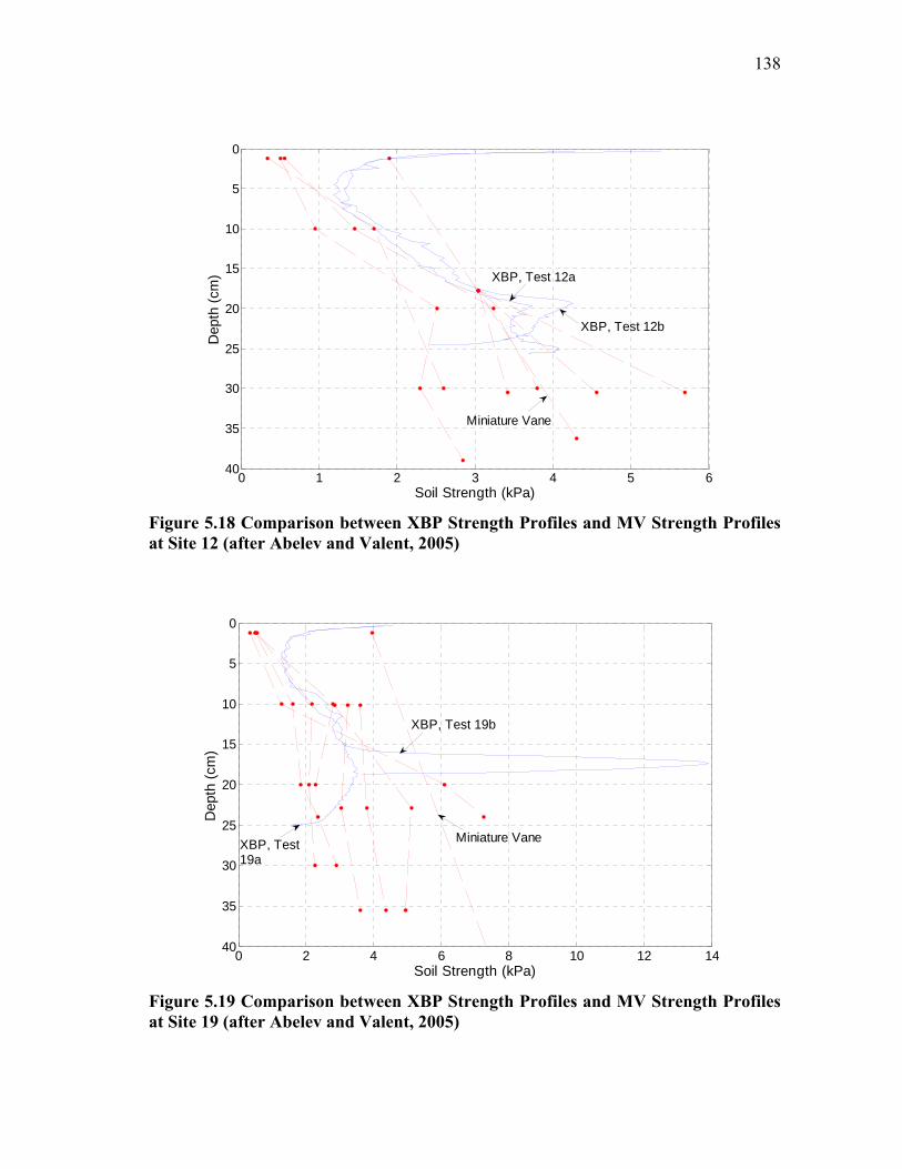
138

0 1 2 3 4 5 6

0

5

10

15

20

25

30

35

40

Dep

th (c

m)

Soil Strength (kPa)

XBP, Test 12b

XBP, Test 12a

Miniature Vane

Figure 5.18 Comparison between XBP Strength Profiles and MV Strength Profiles at Site 12 (after Abelev and Valent, 2005)

0 2 4 6 8 10 12 14

0

5

10

15

20

25

30

35

40

Dep

th (c

m)

Soil Strength (kPa)

XBP, Test 19b

XBP, Test19a

Miniature Vane

Figure 5.19 Comparison between XBP Strength Profiles and MV Strength Profiles at Site 19 (after Abelev and Valent, 2005)

139

As noted above, the existence of thin seams in the soil profiles has been

postulated as a possible cause of the spikes in the interpreted XBP strength profiles.

Indeed, these phenomena spurred an experimental study by Stoll et al. (2004)

investigating the behavior of sands under impact loading using instrumented probes

capable of measuring tip resistance and pore pressures during impact penetration. The

Stoll study showed the rate sensitivity of sands to be much higher than that of the clays

under consideration in this study, and conditions of partial drainage are also a likely

critical factor. High negative pressures measured by the pore water pressure transducers

suggested the tendency for dilation to be related to the apparent strain rate effects.

At present, it appears that more work is needed both to develop a theoretical

framework and to acquire experimental data for analyzing impact penetration in sands.

Accordingly, the framework presented herein for interpreting impact penetration

measurements in soft clays should not be extended to sands until a number of questions

relating to rate effects in sands have been resolved (Aubeny and Shi, 2005b).

140

CHAPTER VI

CONCLUSIONS AND RECOMMENDATIONS*

6.1 Conclusions

There are two aspects in this study: cylinder penetrations and XBP interpretations.

For cylinder penetrations, this study first considers quasi-static collapse loads for a

cylinder embedded in a purely cohesive soil mass. At embedments greater than one-half

diameter, a vertical trench is assumed to exist above the cylinder. The finite element and

plasticity collapse load calculations show the following (Aubeny et al., 2005):

1. For cylinder embedments less than one-half diameter, h/D < 0.5, computed

finite element collapse loads are bracketed by the upper and lower bound

estimates from plasticity theory (Figures 3.15 and 3.16), thus supporting the

validity of the finite element estimates. At shallow embedments, h/D < 0.3,

the lower bound MOC collapse load estimates are virtually in full agreement

with the finite element estimates.

2. For cylinder embedments less than one-half diameter, h/D < 0.5, in a uniform

soil, two velocity fields for upper bound solutions are applied to partially

embedded cylinders, one based on the solution of Randolph and Houlsby

(1984) for a fully embedded translating cylinder, and one based on the

consistent solution of Murff et al. (1989) for a partially embedded cylinder.

* Part of this chapter is reprinted with permission of ASCE from “Collapse loads for a cylinder embedded in trench in cohesive soil.” by C. P. Aubeny, H. Shi and J. D. Murff, 2005, International Journal of Geomechanics, ASCE, scheduled to be published in the 2005.

141

Both solutions (Figure 3.15) provide reasonable estimates of collapse loads,

although the Murff et al. (1989) consistent solution gives somewhat better

overall agreement with finite element estimates. Application of either the

Randolph-Houlsby or the Murff et al. velocity fields to non-uniform soil

strength conditions (Figure 3.16) provides reasonable upper bound collapse

load estimates in the embedment range 5.0/3.0 ≤≤ Dh for the smooth case.

At shallower embedments, the disparity between these upper bound estimates

and both finite element and lower bound MOC solutions becomes

increasingly severe.

3. For cylinder embedments greater than one-half diameter, h/D > 0.5, extension

of the Randolph-Houlsby velocity field to the side wall of the trench and the

ground surface (Figure 3.4), while providing valid upper bound solutions,

tends to substantially over-estimate the finite element collapse load estimates

(Figures 3.17 and 3.18).

4. Collapse loads normalized by the soil strength at the bottom of the cylinder,

ch, are relatively insensitive to strength gradients η. Figure 3.19 shows the

maximum variation in predicted collapse loads due to variation in η is on the

order of 10%.

The study then evaluates the strain rate effects on the collapse loads for a

penetrating cylinder through rate-dependent finite element analyses. A predictive model

for the penetration depth of cylinders was developed subsequently based on a single

particle model. The findings suggest the following (Aubeny and Shi, 2005a):

142

1. If the soil strength c increases semi-logarithmically with strain rate (Eq. 4.1),

the total shearing resistance Fs will, to a reasonable degree of accuracy,

increase in a proportionate manner (Eq. 4.3). Specifically, if ρ0 is the semi-

logarithmic strain rate multiplier for soil strength, then λ0 ≅ ρ0 is a

reasonably accurate estimate of the strain rate multiplier for the total soil

shearing resistance force acting on the cylinder.

2. The approximate power law equations defined by Eq. 3.22 in conjunction

with the approximate approach to accounting for strain rate effects

(Conclusion 1 and Eq. 4.3) provide realistic estimates of the total soil

shearing resistance to penetration of a horizontal cylinder for variable

conditions of velocity v and penetration depth h.

3. Realistic estimates of penetration require a proper accounting of strain rate

effects.

4. The rate-dependent plasticity framework utilized in this study requires an

estimate of a threshold strain rate, below which soil shear strength remains

constant. Limited data are available on this issue, so estimates of this value

entail considerable uncertainty. For the range of conditions considered in this

study, penetration predictions were not sensitive to the magnitude of the

threshold strain rate; however, this observation will not necessarily hold

under all conditions.

The XBP studies were conducted within a framework similar to that of the

cylinder studies. The interpretation is achieved by back-calculating soil strength from

143

impact penetration measurements in soft clays. The development and evaluation of a

framework for relating impact penetration measurements to soil strength lead to the

following conclusions (Aubeny and Shi, 2005b):

1. The highly variable velocity conditions associated with impact penetration

dictate a somewhat different approach to test interpretation than is usually

adopted for constant penetration rate tests. In a constant penetration rate test,

it is reasonable to adopt a single strain rate correction factor relating soil

strength under conditions of penetration to soil strength under other

conditions of interest. However, conditions of variable velocity dictate a

variable strain rate correction (Eq. 4.7) throughout the penetration process.

2. The continuously varying conditions of embedment during XBP penetration

similarly dictate continuous updating of the penetrometer tip resistance

related to soil strength (Eqs. 3.23).

3. Acceleration measurements provide an attractive approach to estimating

strength from impact penetration measurements. In addition to being the

fundamental variable that can be related to soil shearing resistance (Eq. 5.15),

acceleration measurements can be integrated to obtain velocity data for

characterizing rate effects (Eq. 4.7) and depth data for characterizing

embedment effects (Eqs. 3.23).

4. Sediment strength interpreted from XBP measurements agrees reasonably

well with MV shear strength values performed on nearby core samples.

Occasional anomalous spikes in the XBP strength profiles cannot be fully

144

explained at present, but sand seams in the soil profiles are a suspected cause

of this phenomenon.

6.2 Recommendations

The following recommendations can be made for future study (Aubeny and Shi,

2005a):

1. This study assumes a vertical trench is formed in the wake of the advancing

object. In reality the soil will tend to cave in at a certain depth. Therefore, to

which depth this assumption is valid remains an issue to be resolved.

2. The lack of data on the threshold strain rate for very soft normally

consolidated soils is a particular obstacle to using the proposed model with

confidence. It might be noted that if the threshold strain rate is extremely low,

a viscous fluid model could be a preferable model for soil shearing resistance.

3. Much experimental data indicate that the simple semi-logarithmic equation

(Eq. 4.1) relating shear strength to strain rate is not strictly valid over a large

range of strain rates. Accordingly, a need exists for more data and possibly

more comprehensive models.

4. The strength of very soft soils usually cannot be measured directly in tests

having uniform strain and strain rate conditions; i.e., intrusive test methods

(e.g., vane shear, T-bar, cone penetration) are required. Inferring rate-

dependent soil properties from tests involving non-uniform strain rates at

145

present involves considerable ambiguity, pointing to a research need for

improved interpretation of intrusive tests in rate-dependent materials.

5. Further study on the interpretation of the “hard layer effects”, particularly

study on the impact penetration in sands is needed.

6. Although only two geometries (the cylinder and the XBP) were considered in

this research, the methodology described in this study is likely to be feasible

for other geometries, e.g., the spherical penetrometer (Randolph et al., 2000)

etc.

7. Further study taking into account the large strain aspects of the problem may

be considered. The Shallow Strain Path Method (SSPM) proposed by

Sagaseta et al. (1995) combines the Strain Path Method (SPM; Baligh 1985)

with the consideration of the influence of the free surface for shallow

penetration problems by means of image sources and sinks. A strain path

finite element method as described by Teh and Houlsby (1988) may also be

incorporated.

8. Extend study of cylinder penetration to inclined cylinders rotating at some

angular velocity.

146

REFERENCES

Aas, G. (1965). “Study of the effect of vane shape and rate of strain on measured values of in situ shear strength of clays,” Proceedings, 6th International Conference on Soil Mechanics and Foundation Engineering, Montreal, I, 141-145. Abelev, A. (2005). Personal communication, Naval Research Laboratory, Stennis Space Center, Mississippi. Abelev, A. and Valent P. (2005). Personal communication, Naval Research Laboratory, Stennis Space Center, Mississippi. Alberro, J., and Santoyo, E. (1973). “Long term behavior of Mexico City clay.” Proc., 8th International Conference on Soil Mechanics and Foundation Engineering, 1, 1-9. ASTM (2001). “Standard test method for laboratory miniature vane shear test for saturated fine-grained clayey soil.” Annual Book of ASTM Standards, Vol. 04.08, American Society for Testing and Matererials, Philadelphia, 810-815. Aubeny, C.P. (2003). Advanced numerical methods class notes. Department of Civil Engineering, Texas A&M University, College Station, Texas. Aubeny, C.P, and Dunlap, W.A. (2003). “Penetration of cylindrical objects in soft mud.” Proc., Oceans 2003, San Diego, 4, 2068-2073. Aubeny, C.P. and Shi, H. (2005a). “Effect of rate-dependent soil strength on cylinders penetrating into soft clay.” Submitted for publication in IEEE Journal of Oceanic Engineering, Special Issue: Predicting Burial on the Littoral Seafloor. Aubeny, C.P. and Shi, H. (2005b). “Interpretation of impact penetration measurements in soft clays.” Submitted for publication in Journal of Geotechnical and Geoenvironmental Engineering, ASCE. Aubeny, C.P., Shi, H. and Murff, J.D. (2005). “Collapse loads for a cylinder embedded in trench in cohesive soil.” International Journal of Geomechanics, ASCE, scheduled to be published in the 2005. Baligh, M.M. (1985). “Strain path method.” Journal of Geotechnical Engineering, ASCE, 111(9), 1108-1136.

147

Berre, T., and Bjerrum, L. (1973). “Shear strength of normally consolidated clays.” Proc., 8th International Conference on Soil Mechanics and Foundation Engineering, 1, 39-49. Biscontin, G., and Pestana, J.M. (2001). “Influence of peripherial velocity on vane shear strength of an artificial clay.” ASTM. Geotechnical Testing Journal, 24(4), 423-429. Bjerrum, L., Simons, N., and Toblaa, I. (1958). “The effect of time on the shear strength of a soft marine clay.” Proc., Conference on Earth Pressure Problems, 1, 148-158. Bridge, C., Laver, K., Clukey, E., and Evans, T. (2004). “Steel catenary riser touchdown point vertical interaction models.” Offshore Technology Conference, Houston, OTC 16628. Cadling, L., and Odenstad, S. (1950). “The vane borer: an apparatus for determining the shear strength of clay soils directly in the ground.” Royal Swedish Geotechnical Institute, Proceedings, 2, 1-87. Calladine, C.R. (1969). Engineering plasticity, Pergamon Press, Oxford. Casagrande, A., and Wilson, S.D. (1951). “Effect of rate of loading on the strength of clays and shales at constant water content.” Geotechnique, 2(3), 251-263. Chen, W.F. (1975). Limit analysis and soil plasticity, Elsevier, New York. Chu, P.C., Evans, A., Gilles, A., Smith, T., and Taber, V. (2004). “Development of the Navy’s 3D Mine Impact Burial Prediction Model (IMPACT35).” Journal of Counter-Ordnance Technology, 6th International Symposium on Technology and Mine Problem. Davis E.H., and Booker, J.R. (1973). “The effect of increasing strength with depth on the bearing capacity of clays.” Geotechnique, 23(4), 551-563. Drucker, D.C. and Prager, W. (1952). “Soil mechanics and plastic analysis or limit design.” Quarterly of Applied Mathematics, 10, 157-165. Ghazzaly, O.I. and Lim, S.T. (1975). “Experimental investigation of pipeline stability in very soft clays.” Offshore Technology Conference, OTC 2277, 315-326. Halwachs, J.E. (1972). “Analysis of sediment shear strength at varying rates of shear.” Trident Scholar Project Report, TSPR 28, United States Naval Academy. Hight, D. W. (1983). “Laboratory investigations of sea bed clays.” PhD thesis, Imperial College, London, U.K.

148

HKS (2003). ABAQUS Version 6.4 User’s Manuals. Hibbitt, Karlson and Sorensen, Inc. Ladd, C.C., Williams, C.E., Connell, D.H., and Edgers, L. (1972). “Engineering properties of soft foundation clays at two south Louisiana levee sites.” Research Report No. R72-26, Massachusetts Institute of Technology, Cambridge, Massachusetts. Lefebvre, G., and LeBoeuf, D. (1987). “Rate effects and cyclic loading of sensitive clays.” Journal of Geotechnical Engineering., ASCE, 113(5), 476-489. Martin (2001). “Vertical bearing capacity of skirted circular foundations on Tresca soil.” 15th International Conference on Soil Mechanics and Geotechnical Engineering, Istanbul, International Society for Soil Mechanics and Geotechnical Engineering, 743-746. Munim, M. (2003). “Experimental investigation of mine penetration in soft sediments.” MS thesis, Department of Civil Engineering, Texas A&M University, College Station, Texas. Murff, J.D. (1978). “Upper bound analysis of incompressible, anisotropic media.” Proc., 15th Annual Meeting of the Society of Engineering Science, 521-526. Murff, J.D. (1980). “Vane shear testing of anisotropic, cohesive soils.” International Journal for Numerical and Analytical Methods in Geomechanics, 4, 285-289. Murff, J.D. (2002). Geo-mechanics class notes. Department of Civil Engineering, Texas A&M University, College Station, Texas. Murff, J.D. (2003). Advanced numerical methods class notes. Department of Civil Engineering, Texas A&M University, College Station, Texas. Murff, J.D., Wagner, D.A., and Randolph, M.F. (1989). “Pipe penetration in cohesive soil.” Geotechnique, 39(2), 213-229. Perlow, M., and Richards, A.F. (1977). “Influence of shear velocity on vane shear strength.” Journal of the Geotechnical Engineering Division, ASCE, 103(GT1), 19-32. Randolph, M.F., and Houlsby, G.T. (1984). “The limiting pressure on a circular pile loaded laterally in cohesive soil.” Geotechnique, 34(4), 613-623. Randolph, M.F., Martin, C.M. and Hu, Y. (2000). “Limiting resistance of a spherical penetrometer in cohesive material.” Geotechnique, 50(5), 573-582. Reddy, J.N. (1993). An introduction to the finite element method, McGraw-Hill, New York.

149

Richardson, A.M. (1963). “The relationship of the effective stress-strain behavior of a saturated clay to the rate of strain.” ScD thesis, Massachusetts Institute of Technology, Cambridge, Massachusetts. Richardson, A.M., and Whitman, R.V. (1963). “Effect of strain-rate upon undrained shear resistance of a saturated remoulded fat clay.” Geotechnique, 13(4), 310-324. Roy, M., and LeBlanc, A. (1988). “The in-situ measurement of the undrained shear strength of clays using the field vane.” Vane Shear Strength Testing in Soils: Field and Laboratory Studies, ASTM STP 1014, A.F. Richards, Ed., Philadelphia, 117-128. Sagaseta, C., Whittle, A., and Santagata, M. (1995). “Deformation analysis of shallow penetration in saturated clay.” Research Report R94-09, Massachusetts Institute of Technology, Cambridge, Massachusetts. Schapery, R.A., and Dunlap, W.A. (1978). “Prediction of storm-induced sea bottom movement and platform forces.” Offshore Technology Conference, Houston, OTC 3259. Schapery, R.A. and Dunlap, W.A. (1984). “Theoretical and experimental investigation of mud forces on offshore pipelines.” Report No. RF4534-1, Texas A&M University, College Station, Texas. Sharifounnasab, M., and Ullrich, R.C. (1985). “Rate of shear effects on vane shear strength.” Journal of Geotechnical Engineering, ASCE, 111(1), 135-139. Sheahan, T.C., Ladd, C.C., and Germaine, J.T. (1996). “Rate-dependent undrained shear strength behavior of saturated clay.” Journal of Geotechnical Engineering, ASCE,122(2), 99-108. Skempton, A.W. (1948). “Vane tests in the alluvial plain of the river forth near Grangemouth.” Geotechnique, 1(2), 111-124. Small, S.W., Tambuvello, R. D., and Piaseckyj, P. J. (1971). “Submarine pipeline support by marine sediments.” Offshore Technology Conference, Houston, OTC 1357, 309-318. Smith, A.D., and Richards, A.F. (1975). “Vane shear strength at two high rotation rates,” Proc., Civil Engineering in the Oceans III, Newark, Delaware, Vol. I, 421-433. Sokolovskii, V.V. (1965). Statics of granular media, Pergamon Press, Oxford.

150

Stoll, R.D., Sun, Y.F. and Bitte, I. (2004). Measuring Sea Bed Properties Using Static and Dynamic Penetrometers, Lamont-Doherty Earth Observatory of Columbia University, New York. Teh, C.I., and Houlsby, G.T. (1988). “Analysis of the cone penetration test by the strain path method.” Proc., 6th International Conference on Numerical and Analytical Methods in Geo-mechanics, Innsbruck, 2, 1443-1448. Terzaghi, K. (1943). Theoretical soil mechanics, Wiley, New York. Torstensson, B.A. (1977). “Time-dependent effects in the field vane test.” International Symposium on Soft Clay, Bangkok, 387-397. Vaid, Y.P., and Campanella, R.G. (1977). “Time-dependent behavior of undisturbed clay.” Journal of the Geotechnical Engineering Division, ASCE, 103(7), 693-709. Valent, P. (2003). Personal communication, Naval Research Laboratory, Stennis Space Center, Mississippi. Whitney, M.J., and Rodin, G.J. (2001). “Force-velocity relationships for rigid bodies translating through unbounded shear-thinning power-law fluids.” International Journal of Non-Linear Mechanics, 36, 947-953. Wiesel, C.E. (1973). “Some factors influencing in-situ vane tests results.” Proc., 8th International Conference on Soil Mechanics and Foundation Engineering, Moscow, Vol. 1.2, 475-479. Willis, N.R.T. and West, P.T.J. (2001). “Interaction between deepwater catenary risers and a soft seabed: large scale sea trials.” Offshore Technology Conference, Houston, OTC 13113. Yao, Z. (2003). “Numerical simulations of mine penetration in soft sediments.” MS thesis, Department of Civil Engineering., Texas A&M University, College Station, Texas.

151

APPENDIX A

MATLAB PROGRAM: MOC_CYLINDER

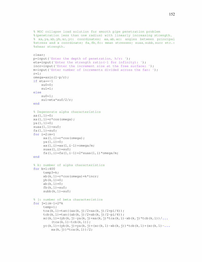
152

% MOC collapse load solution for smooth pipe penetration problem %(penetration less than one radius) with linearly increasing strength. % xa,ya,xb,yb,xc,yc: coordinates; aa,ab,ac: angles between principal %stress and x coordinate; fa,fb,fc: mean stresses; suaa,subb,succ etc.: %shear strength. clear; p=input('Enter the depth of penetration, h/r: '); eta=input('Enter the strength ratio(-1 for infinity): '); incr=input('Enter the increment size at the free surface: '); m=input('Enter number of increments divided across the fan: '); r=1; omega=asin(1-p/r); if eta==-1 su0=0; su1=1; else su0=1; su1=eta*su0/2/r; end % Degenerate alpha characteristics aa(1,1)=0; xa(1,1)=r*cos(omega); ya(1,1)=0; suaa(1,1)=su0; fa(1,1)=su0; for i=2:m+1 xa(1,i)=r*cos(omega); ya(1,i)=0; aa(1,i)=aa(1,i-1)+omega/m; suaa(1,i)=su0; fa(1,i)=fa(1,i-1)+2*suaa(1,i)*omega/m; end % k: number of alpha characteristics for k=1:400 temp3=k; xb(k,1)=r*cos(omega)+k*incr; yb(k,1)=0; ab(k,1)=0; fb(k,1)=su0; subb(k,1)=su0; % j: number of beta characteristics for j=1:m-1+2*k temp=1; tca(k,1)=tan((aa(k,j)/2+aa(k,j)/2+pi/4)); tcb(k,1)=tan((ab(k,j)/2+ab(k,j)/2-pi/4)); xc(k,1)=(yb(k,j)-ya(k,j)+xa(k,j)*tca(k,1)-xb(k,j)*tcb(k,1))/... (tca(k,1)-tcb(k,1)); yc(k,1)=(yb(k,j)+ya(k,j)+(xc(k,1)-xb(k,j))*tcb(k,1)+(xc(k,1)-... xa(k,j))*tca(k,1))/2;

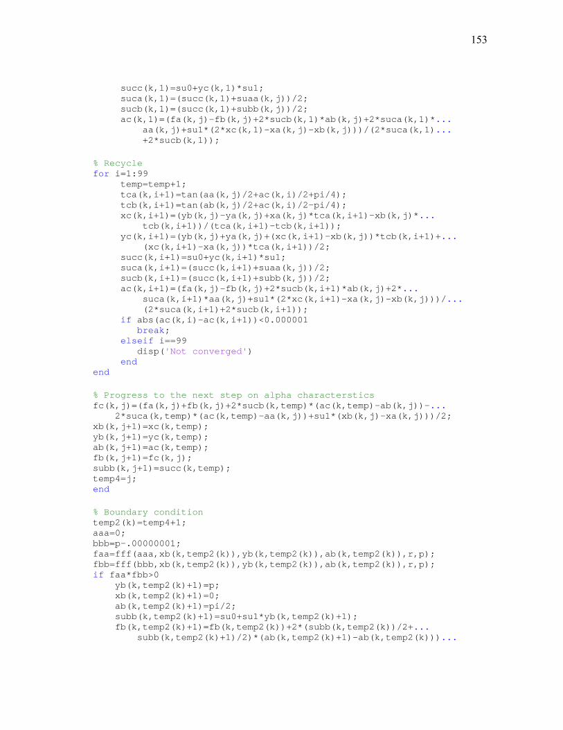
153

succ(k,1)=su0+yc(k,1)*su1; suca(k,1)=(succ(k,1)+suaa(k,j))/2; sucb(k,1)=(succ(k,1)+subb(k,j))/2; ac(k,1)=(fa(k,j)-fb(k,j)+2*sucb(k,1)*ab(k,j)+2*suca(k,1)*... aa(k,j)+su1*(2*xc(k,1)-xa(k,j)-xb(k,j)))/(2*suca(k,1)... +2*sucb(k,1)); % Recycle for i=1:99 temp=temp+1; tca(k,i+1)=tan(aa(k,j)/2+ac(k,i)/2+pi/4); tcb(k,i+1)=tan(ab(k,j)/2+ac(k,i)/2-pi/4); xc(k,i+1)=(yb(k,j)-ya(k,j)+xa(k,j)*tca(k,i+1)-xb(k,j)*... tcb(k,i+1))/(tca(k,i+1)-tcb(k,i+1)); yc(k,i+1)=(yb(k,j)+ya(k,j)+(xc(k,i+1)-xb(k,j))*tcb(k,i+1)+... (xc(k,i+1)-xa(k,j))*tca(k,i+1))/2; succ(k,i+1)=su0+yc(k,i+1)*su1; suca(k,i+1)=(succ(k,i+1)+suaa(k,j))/2; sucb(k,i+1)=(succ(k,i+1)+subb(k,j))/2; ac(k,i+1)=(fa(k,j)-fb(k,j)+2*sucb(k,i+1)*ab(k,j)+2*... suca(k,i+1)*aa(k,j)+su1*(2*xc(k,i+1)-xa(k,j)-xb(k,j)))/... (2*suca(k,i+1)+2*sucb(k,i+1)); if abs(ac(k,i)-ac(k,i+1))<0.000001 break; elseif i==99 disp('Not converged') end end % Progress to the next step on alpha characterstics fc(k,j)=(fa(k,j)+fb(k,j)+2*sucb(k,temp)*(ac(k,temp)-ab(k,j))-... 2*suca(k,temp)*(ac(k,temp)-aa(k,j))+su1*(xb(k,j)-xa(k,j)))/2; xb(k,j+1)=xc(k,temp); yb(k,j+1)=yc(k,temp); ab(k,j+1)=ac(k,temp); fb(k,j+1)=fc(k,j); subb(k,j+1)=succ(k,temp); temp4=j; end % Boundary condition temp2(k)=temp4+1; aaa=0; bbb=p-.00000001; faa=fff(aaa,xb(k,temp2(k)),yb(k,temp2(k)),ab(k,temp2(k)),r,p); fbb=fff(bbb,xb(k,temp2(k)),yb(k,temp2(k)),ab(k,temp2(k)),r,p); if faa*fbb>0 yb(k,temp2(k)+1)=p; xb(k,temp2(k)+1)=0; ab(k,temp2(k)+1)=pi/2; subb(k,temp2(k)+1)=su0+su1*yb(k,temp2(k)+1); fb(k,temp2(k)+1)=fb(k,temp2(k))+2*(subb(k,temp2(k))/2+... subb(k,temp2(k)+1)/2)*(ab(k,temp2(k)+1)-ab(k,temp2(k)))...

154

-su1*(xb(k,temp2(k)+1)-xb(k,temp2(k))); ff(k)=fb(k,temp2(k)+1)+subb(k,temp2(k)+1); hold on; plot(xb(k,:),-yb(k,:)); break; end cc=(aaa+bbb)/2; fcc=fff(cc,xb(k,temp2(k)),yb(k,temp2(k)),ab(k,temp2(k)),r,p); while abs(fcc)>=.000001 if fcc*faa<0 bbb=cc; cc=(aaa+bbb)/2; fcc=fff(cc,xb(k,temp2(k)),yb(k,temp2(k)),ab(k,temp2(k)),r,p); fbb=fff(bbb,xb(k,temp2(k)),yb(k,temp2(k)),ab(k,temp2(k)),r,p); elseif fcc*fbb<0 aaa=cc; cc=(bbb+aaa)/2; fcc=fff(cc,xb(k,temp2(k)),yb(k,temp2(k)),ab(k,temp2(k)),r,p); faa=fff(aaa,xb(k,temp2(k)),yb(k,temp2(k)),ab(k,temp2(k)),r,p); else disp('Bottom of cylinder not reached'); break; end end yb(k,temp2(k)+1)=cc; xb(k,temp2(k)+1)=sqrt(r*r-(cc+r-p)^2); ab(k,temp2(k)+1)=atan((cc+r-p)/xb(k,temp2(k)+1)); subb(k,temp2(k)+1)=su0+su1*yb(k,temp2(k)+1); fb(k,temp2(k)+1)=fb(k,temp2(k))+2*(subb(k,temp2(k))/2+... subb(k,temp2(k)+1)/2)*(ab(k,temp2(k)+1)-ab(k,temp2(k)))-... su1*(xb(k,temp2(k)+1)-xb(k,temp2(k))); ff(k)=fb(k,temp2(k)+1)+subb(k,temp2(k)+1); % Plot alpha characteristics figure(1) hold on; axis equal; plot(xb(k,:),-yb(k,:)) % Progress to the next alpha characteristics for j=1:temp2(k)+1 xa(k+1,j)=xb(k,j); ya(k+1,j)=yb(k,j); aa(k+1,j)=ab(k,j); fa(k+1,j)=fb(k,j); suaa(k+1,j)=subb(k,j); end end % Calculate collapse load f1=ff(1)*sin(ab(1,temp2(1)+1))*r*(ab(1,temp2(1)+1)-aa(1,21)); for i=1:temp3-1 f1=f1+ff(i+1)*sin(ab(i+1,temp2(i+1)+1))*...

155

(ab(i+1,temp2(i+1)+1)-ab(i,temp2(i)+1)); end f2=fa(1,21)*sin(aa(1,21))*r*(ab(1,temp2(1)+1)-aa(1,21)); for i=1:temp3-1 f2=f2+ff(i)*sin(ab(i,temp2(i)+1))*(ab(i+1,temp2(i+1)+1)-... ab(i,temp2(i)+1)); end f=(f1+f2)/2; % Normalize by the soil strength at the bottom of cylinder cavg=su0+su1*p; disp(' '); disp('Normalized collapse load'); fv=2*f/2/r/cavg % Plot beta characteristics for k=1:temp3-1 for j=1:temp2(k)+1 xx(1)=xb(k,j); yy(1)=yb(k,j); xx(2)=xb(k+1,j+1); yy(2)=yb(k+1,j+1); figure(1) hold on; plot(xx,-yy); end end xs(1)=xa(1,1); ys(1)=ya(1,1); xs(2)=xb(1,2); ys(2)=yb(1,2); figure(1) hold on; plot(xs,-ys); % Plot cylinder yp=linspace(-p,2-p,100); for i=1:100 xp(i)=sqrt(r*r-(yp(i)-r+p)^2); end figure(1); hold on; axis equal; plot(xp,yp); % Plot free surface x00=sqrt(r*r-(r-p)^2); xh=linspace(x00,2.8,100); yh(1:100)=0; figure(1) hold on; plot(xh,yh) axis([0,2.8,-2,2]);

156

function[f]=fff(y,xc,yc,ac,r,p) x=sqrt(r*r-(y+r-p)^2); af=atan((y+r-p)/x); f=yc+(x-xc)*tan((atan((y+r-p)/x)+ac)/2-pi/4)-y;

157

APPENDIX B

MATLAB PROGRAM: RH_CYLINDER

158

% Program for modified Randolph-Houlsby upperbound for cylinder %penetration with linearly increasing strength clear; % Input data p=input('Enter the depth of penetration, h/r: '); eta=input('Enter the strength ratio(-1 for infinity): '); delta=input('Enter the adhesion angle(0~pi/2): '); %note: enter pi/2-0.000001 for pi/2 to avoid singularity r0=1; ksai=pi/4-delta/2; v0=1; if eta==-1 su0=0; su1=1; else su0=1; su1=eta*su0/2/r0; end if p>r0 omega=0; else omega=asin((r0-p)/r0); end % Interface AF if p<=r0 a1=r0*cos(delta/2)-r0*sin(omega); b1=r0*cos(delta/2)-r0*sin(omega)+r0*sin(delta/2); elseif p>r0 a1=p-r0+r0*cos(delta/2); b1=p-r0+r0*cos(delta/2)+r0*sin(delta/2); end w(1)=su0*v0*(b1-a1)+su1*v0*(b1*b1-a1*a1)/2; % Interface ABC w(2)=intABC(ksai,v0,r0,su0,su1,delta,omega,pi/2-delta/2,p,omega); % Interface CDE rr1=r0*(sqrt(2)*sin(delta/2)+(pi/2-delta/2-omega)*cos(ksai)); if p<=r0 w(3)=v0*su0/sqrt(2)*rr1*(delta/2+omega+pi/4)+... su1*rr1*rr1*v0/sqrt(2)*(1-cos(pi/4+delta/2+omega)); else w(3)=v0*su0/sqrt(2)*rr1*(delta/2+omega+pi/4)+su1*(p-r0)*... v0/sqrt(2)*rr1*(delta/2+omega+pi/4)+su1*rr1*rr1*v0/... sqrt(2)*(1-cos(pi/4+delta/2+omega)); end % Interface FGH w(4)=intFGH(ksai,v0,r0,su0,su1,delta,omega,pi/2-delta/2,p,omega);

159

% Interface HIJ rr2=r0*(pi/2-delta/2-omega)*cos(ksai); vt=v0*cos(delta/2)/cos(ksai)-v0/sqrt(2); if p<=r0 w(5)=vt*su0*rr2*(delta/2+omega+pi/4)+su1*rr2*rr2*vt*... (1-cos(pi/4+delta/2+omega)); else w(5)=vt*su0*rr2*(delta/2+omega+pi/4)+vt*su1*(p-r0)*rr2*... (delta/2+omega+pi/4)+su1*rr2*rr2*vt*(1-... cos(pi/4+delta/2+omega)); end % Interface FKQ w(6)=int1(ksai,v0,r0,su0,su1,delta,omega,pi/2-delta/2,p,omega); % Region ABCHGF w(7)=dblint1(ksai,v0,r0,su0,su1,omega,pi/2-delta/2,delta,p,omega); % Region CDEJIH r3=r0*(pi/2-delta/2-omega)*cos(ksai); r4=r0*(sqrt(2)*sin(delta/2)+(pi/2-delta/2-omega)*cos(ksai)); w(8)=dblint4(ksai,v0,r0,su0,su1,0,pi/4+delta/2+omega,r3,r4,p,1); % Region FGHQK w(9)=dblint2(ksai,v0,r0,su0,su1,omega,pi/2-delta/2,p,omega); % Region HIJQ w(10)=dblint3(ksai,v0,r0,su0,su1,omega,pi/2-delta/2,0,pi/4+... delta/2+omega,omega,p,1); if (p>r0&p<=r3+r0) % Region EOMJ beta1=asin((p-r0)/r4); w(11)=dblint4(ksai,v0,r0,su0,su1,0,beta1,r3,r4,p,2); % Region OMN beta2=asin((p-r0)/r3); w(12)=dblint5(ksai,v0,r0,su0,su1,beta1,beta2,delta,omega,p); % Region JNQ w(13)=dblint3(ksai,v0,r0,su0,su1,omega,pi/2-delta/2,0,beta2,omega,p,2); % Region NQP w(14)=dblint6(ksai,v0,r0,su0,su1,beta2,pi/2,omega,p); % Interface EO r23=r0*(sqrt(2)*sin(delta/2)+(pi/2-delta/2-omega)*cos(ksai)); w(15)=(su0+su1*(p-r0))*v0/sqrt(2)*r23*beta1+su1*r23*r23*v0/... sqrt(2)*(cos(beta1)-1);

160

% Interface JMN r15=r0*(pi/2-delta/2-omega)*cos(ksai); w(16)=(su0+su1*(p-r0))*vt*r15*beta2+su1*r15*r15*vt*(cos(beta2)-1); elseif (p>r3+r0&p<r4+r0) % Region EOMJ beta1=asin((p-r0)/r4); w(11)=dblint4(ksai,v0,r0,su0,su1,0,beta1,r3,r4,p,2); % Region OMN w(12)=dblint5(ksai,v0,r0,su0,su1,beta1,pi/2,delta,omega,p); % Region JNQ w(13)=dblint3(ksai,v0,r0,su0,su1,omega,pi/2-delta/2,0,pi/2,omega,p,2); % Interface EO r23=r0*(sqrt(2)*sin(delta/2)+(pi/2-delta/2-omega)*cos(ksai)); w(14)=(su0+su1*(p-r0))*v0/sqrt(2)*r23*beta1+su1*r23*r23*v0/... sqrt(2)*(cos(beta1)-1); % Interface JMN r15=r0*(pi/2-delta/2-omega)*cos(ksai); w(15)=(su0+su1*(p-r0))*vt*r15*pi/2+su1*r15*r15*vt*(cos(pi/2)-1); elseif p>=r4+r0 % Region EOMJ w(11)=dblint4(ksai,v0,r0,su0,su1,0,pi/2,r3,r4,p,2); % Region JNQ w(12)=dblint3(ksai,v0,r0,su0,su1,omega,pi/2-delta/2,0,pi/2,omega,p,2); % Interface EO r23=r0*(sqrt(2)*sin(delta/2)+(pi/2-delta/2-omega)*cos(ksai)); w(13)=(su0+su1*(p-r0))*v0/sqrt(2)*r23*pi/2+su1*r23*r23*v0/... sqrt(2)*(cos(pi/2)-1); % Interface JMN r15=r0*(pi/2-delta/2-omega)*cos(ksai); w(14)=(su0+su1*(p-r0))*vt*r15*pi/2+su1*r15*r15*vt*(cos(pi/2)-1); end % Calculate collapse load fv=2*sum(w(:))/v0; cp=su0+su1*p; disp(' '); disp('Normalized collapse load: '); fv=fv/2/r0/cp

161

% Integration function for interface ABC function[sum2]=intABC(ksai,v0,r0,su0,su1,delta,a,b,p,omega) sum2=0; xsum=0; d=(b-a)/100; for theta2=a:d:b xsum=xsum+1; if p<=r0 z=r0*sin(theta2)-r0*sin(omega)+cos(theta2-omega)*(r0*... sqrt(2)*sin(delta/2)+r0*(pi/2-delta/2-theta2)*cos(ksai)); elseif p>r0 z=p-r0+r0*sin(theta2)+cos(theta2-omega)*(r0*sqrt(2)*... sin(delta/2)+r0*(pi/2-delta/2-theta2)*cos(ksai)); end c2=su0+su1*z; v2=v0/sqrt(2); w(xsum)=c2*v0/sqrt(2)*r0*(sqrt(2)*sin(delta/2)+sin(ksai)+... (pi/2-delta/2-theta2)*cos(ksai)); end for i=1:xsum sum2=sum2+w(i)*d; end sum2=sum2-w(1)*d/2-w(xsum)*d/2;

162

% Integration function for interface FGH function[sum2]=intFGH(ksai,v0,r0,su0,su1,delta,a,b,p,omega) sum2=0; xsum=0; d=(b-a)/100; for theta2=a:d:b xsum=xsum+1; if p<=r0 z=r0*sin(theta2)-r0*sin(omega)+cos(theta2-omega)*r0*... (pi/2-delta/2-theta2)*cos(ksai); elseif p>r0 z=p-r0+r0*sin(theta2)+cos(theta2-omega)*r0*(pi/2-... delta/2-theta2)*cos(ksai); end c3=su0+su1*z; vt=v0*cos(delta/2)/cos(ksai)-v0/sqrt(2); w(xsum)=c3*vt*r0*(sin(ksai)+(pi/2-delta/2-theta2)*cos(ksai)); end for i=1:xsum sum2=sum2+w(i)*d; end sum2=sum2-w(1)*d/2-w(xsum)*d/2;

163

% Integration function for region FKQ function[sum2]=int1(ksai,v0,r0,su0,su1,delta,a,b,p,omega) sum2=0; xsum=0; d=(b-a)/100; for theta1=a:d:b xsum=xsum+1; if p<=r0 z=r0*sin(theta1)-r0*sin(omega); elseif p>r0 z=r0*sin(theta1)+p-r0; end c3=su0+su1*z; v3=v0*(cos(theta1)+sin(theta1)*tan(ksai)); w(xsum)=c3*sin(delta)*v3*r0; end for i=1:xsum sum2=sum2+w(i)*d; end sum2=sum2-w(1)*d/2-w(xsum)*d/2;

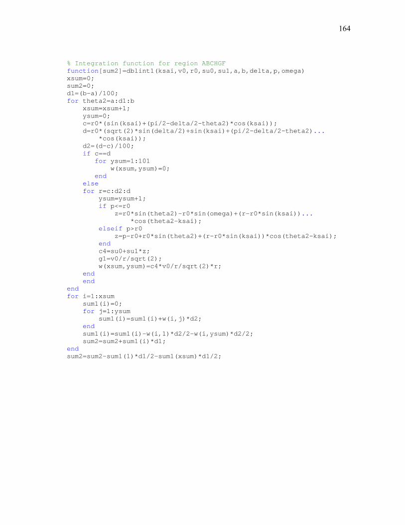
164

% Integration function for region ABCHGF function[sum2]=dblint1(ksai,v0,r0,su0,su1,a,b,delta,p,omega) xsum=0; sum2=0; d1=(b-a)/100; for theta2=a:d1:b xsum=xsum+1; ysum=0; c=r0*(sin(ksai)+(pi/2-delta/2-theta2)*cos(ksai)); d=r0*(sqrt(2)*sin(delta/2)+sin(ksai)+(pi/2-delta/2-theta2)... *cos(ksai)); d2=(d-c)/100; if c==d for ysum=1:101 w(xsum,ysum)=0; end else for r=c:d2:d ysum=ysum+1; if p<=r0 z=r0*sin(theta2)-r0*sin(omega)+(r-r0*sin(ksai))... *cos(theta2-ksai); elseif p>r0 z=p-r0+r0*sin(theta2)+(r-r0*sin(ksai))*cos(theta2-ksai); end c4=su0+su1*z; g1=v0/r/sqrt(2); w(xsum,ysum)=c4*v0/r/sqrt(2)*r; end end end for i=1:xsum sum1(i)=0; for j=1:ysum sum1(i)=sum1(i)+w(i,j)*d2; end sum1(i)=sum1(i)-w(i,1)*d2/2-w(i,ysum)*d2/2; sum2=sum2+sum1(i)*d1; end sum2=sum2-sum1(1)*d1/2-sum1(xsum)*d1/2;

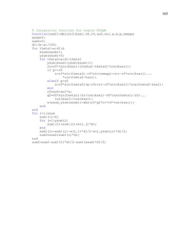
165

% Integration function for region FGHQK function[sum2]=dblint2(ksai,v0,r0,su0,su1,a,b,p,omega) xsum=0; sum2=0; d1=(b-a)/100; for theta1=a:d1:b xsum=xsum+1; ysum(xsum)=0; for theta2=a:d1:theta1 ysum(xsum)=ysum(xsum)+1; rr=r0*(sin(ksai)+(theta1-theta2)*cos(ksai)); if p<=r0 z=r0*sin(theta2)-r0*sin(omega)+(rr-r0*sin(ksai))... *cos(theta2-ksai); elseif p>r0 z=r0*sin(theta2)+p-r0+(rr-r0*sin(ksai))*cos(theta2-ksai); end c5=su0+su1*z; g2=v0*sin(theta1)/rr/cos(ksai)-v0*cos(theta1)/r0/... cos(ksai)/cos(ksai); w(xsum,ysum(xsum))=abs(c5*g2*rr*r0*cos(ksai)); end end for i=1:xsum sum1(i)=0; for j=1:ysum(i) sum1(i)=sum1(i)+w(i,j)*d1; end sum1(i)=sum1(i)-w(i,1)*d1/2-w(i,ysum(i))*d1/2; sum2=sum2+sum1(i)*d1; end sum2=sum2-sum1(1)*d1/2-sum1(xsum)*d1/2;

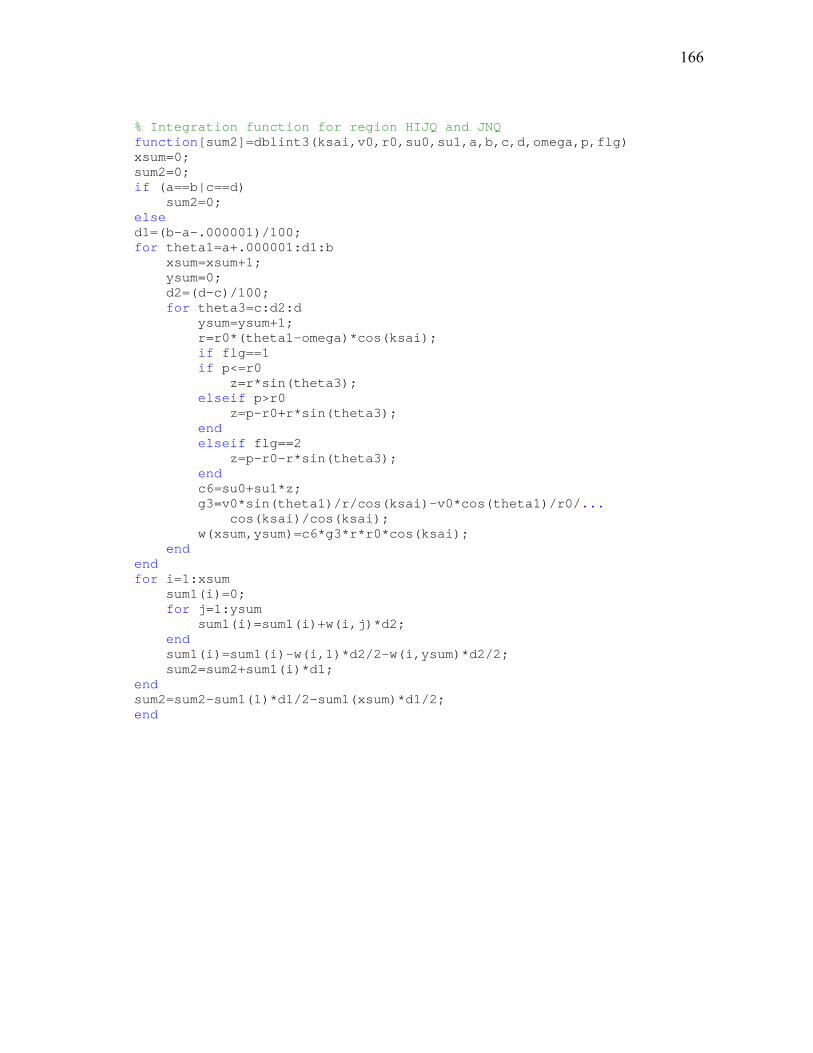
166

% Integration function for region HIJQ and JNQ function[sum2]=dblint3(ksai,v0,r0,su0,su1,a,b,c,d,omega,p,flg) xsum=0; sum2=0; if (a==b|c==d) sum2=0; else d1=(b-a-.000001)/100; for theta1=a+.000001:d1:b xsum=xsum+1; ysum=0; d2=(d-c)/100; for theta3=c:d2:d ysum=ysum+1; r=r0*(theta1-omega)*cos(ksai); if flg==1 if p<=r0 z=r*sin(theta3); elseif p>r0 z=p-r0+r*sin(theta3); end elseif flg==2 z=p-r0-r*sin(theta3); end c6=su0+su1*z; g3=v0*sin(theta1)/r/cos(ksai)-v0*cos(theta1)/r0/... cos(ksai)/cos(ksai); w(xsum,ysum)=c6*g3*r*r0*cos(ksai); end end for i=1:xsum sum1(i)=0; for j=1:ysum sum1(i)=sum1(i)+w(i,j)*d2; end sum1(i)=sum1(i)-w(i,1)*d2/2-w(i,ysum)*d2/2; sum2=sum2+sum1(i)*d1; end sum2=sum2-sum1(1)*d1/2-sum1(xsum)*d1/2; end

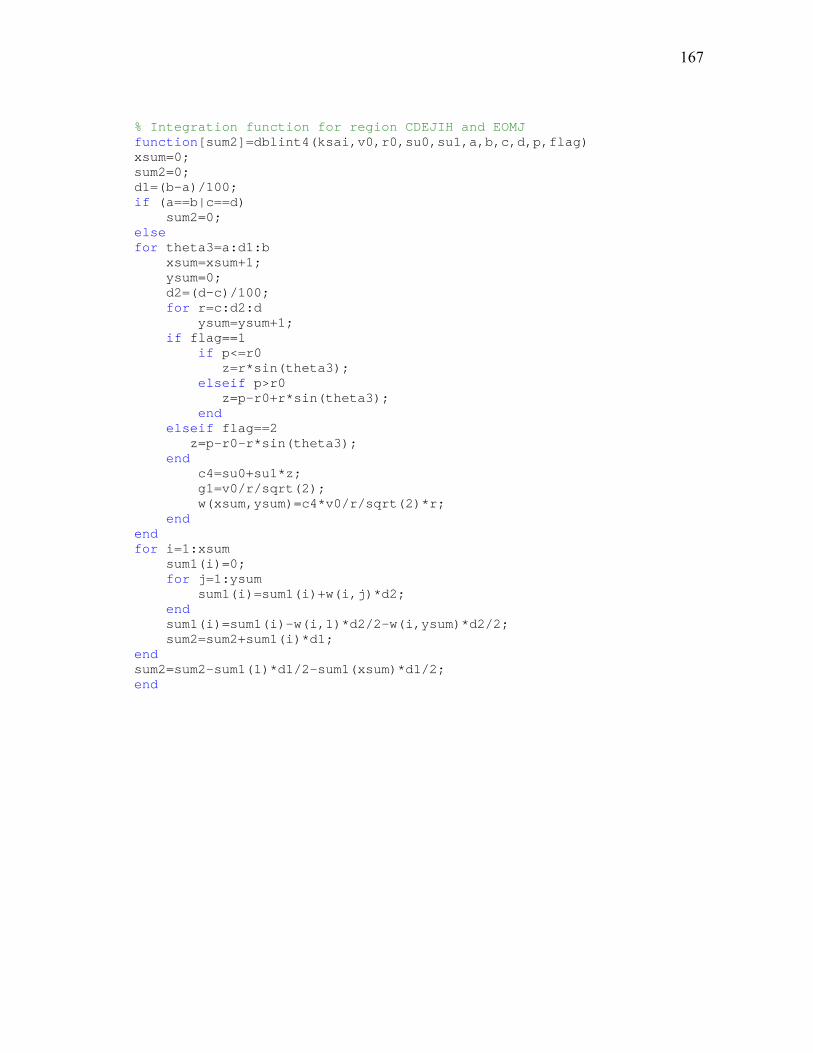
167

% Integration function for region CDEJIH and EOMJ function[sum2]=dblint4(ksai,v0,r0,su0,su1,a,b,c,d,p,flag) xsum=0; sum2=0; d1=(b-a)/100; if (a==b|c==d) sum2=0; else for theta3=a:d1:b xsum=xsum+1; ysum=0; d2=(d-c)/100; for r=c:d2:d ysum=ysum+1; if flag==1 if p<=r0 z=r*sin(theta3); elseif p>r0 z=p-r0+r*sin(theta3); end elseif flag==2 z=p-r0-r*sin(theta3); end c4=su0+su1*z; g1=v0/r/sqrt(2); w(xsum,ysum)=c4*v0/r/sqrt(2)*r; end end for i=1:xsum sum1(i)=0; for j=1:ysum sum1(i)=sum1(i)+w(i,j)*d2; end sum1(i)=sum1(i)-w(i,1)*d2/2-w(i,ysum)*d2/2; sum2=sum2+sum1(i)*d1; end sum2=sum2-sum1(1)*d1/2-sum1(xsum)*d1/2; end

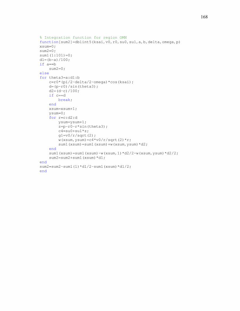
168

% Integration function for region OMN function[sum2]=dblint5(ksai,v0,r0,su0,su1,a,b,delta,omega,p) xsum=0; sum2=0; sum1(1:101)=0; d1=(b-a)/100; if a==b sum2=0; else for theta3=a:d1:b c=r0*(pi/2-delta/2-omega)*cos(ksai); d=(p-r0)/sin(theta3); d2=(d-c)/100; if c==d break; end xsum=xsum+1; ysum=0; for r=c:d2:d ysum=ysum+1; z=p-r0-r*sin(theta3); c4=su0+su1*z; g1=v0/r/sqrt(2); w(xsum,ysum)=c4*v0/r/sqrt(2)*r; sum1(xsum)=sum1(xsum)+w(xsum,ysum)*d2; end sum1(xsum)=sum1(xsum)-w(xsum,1)*d2/2-w(xsum,ysum)*d2/2; sum2=sum2+sum1(xsum)*d1; end sum2=sum2-sum1(1)*d1/2-sum1(xsum)*d1/2; end

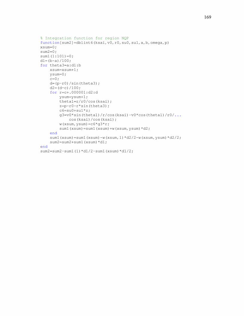
169

% Integration function for region NQP function[sum2]=dblint6(ksai,v0,r0,su0,su1,a,b,omega,p) xsum=0; sum2=0; sum1(1:101)=0; d1=(b-a)/100; for theta3=a:d1:b xsum=xsum+1; ysum=0; c=0; d=(p-r0)/sin(theta3); d2=(d-c)/100; for r=c+.000001:d2:d ysum=ysum+1; theta1=r/r0/cos(ksai); z=p-r0-r*sin(theta3); c6=su0+su1*z; g3=v0*sin(theta1)/r/cos(ksai)-v0*cos(theta1)/r0/... cos(ksai)/cos(ksai); w(xsum,ysum)=c6*g3*r; sum1(xsum)=sum1(xsum)+w(xsum,ysum)*d2; end sum1(xsum)=sum1(xsum)-w(xsum,1)*d2/2-w(xsum,ysum)*d2/2; sum2=sum2+sum1(xsum)*d1; end sum2=sum2-sum1(1)*d1/2-sum1(xsum)*d1/2;

170

APPENDIX C

MATLAB PROGRAM: CU_CYLINDER∗

∗ Functions are the same as defined in Appendix B.

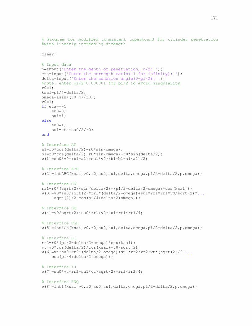
171

% Program for modified consistent upperbound for cylinder penetration %with linearly increasing strength clear; % Input data p=input('Enter the depth of penetration, h/r: '); eta=input('Enter the strength ratio(-1 for infinity): '); delta=input('Enter the adhesion angle(0~pi/2): '); %note: enter pi/2-0.000001 for pi/2 to avoid singularity r0=1; ksai=pi/4-delta/2; omega=asin((r0-p)/r0); v0=1; if eta==-1 su0=0; su1=1; else su0=1; su1=eta*su0/2/r0; end % Interface AF a1=r0*cos(delta/2)-r0*sin(omega); b1=r0*cos(delta/2)-r0*sin(omega)+r0*sin(delta/2); w(1)=su0*v0*(b1-a1)+su1*v0*(b1*b1-a1*a1)/2; % Interface ABC w(2)=intABC(ksai,v0,r0,su0,su1,delta,omega,pi/2-delta/2,p,omega); % Interface CD rr1=r0*(sqrt(2)*sin(delta/2)+(pi/2-delta/2-omega)*cos(ksai)); w(3)=v0*su0/sqrt(2)*rr1*(delta/2+omega)+su1*rr1*rr1*v0/sqrt(2)*... (sqrt(2)/2-cos(pi/4+delta/2+omega)); % Interface DE w(4)=v0/sqrt(2)*su0*rr1+v0*su1*rr1*rr1/4; % Interface FGH w(5)=intFGH(ksai,v0,r0,su0,su1,delta,omega,pi/2-delta/2,p,omega); % Interface HI rr2=r0*(pi/2-delta/2-omega)*cos(ksai); vt=v0*cos(delta/2)/cos(ksai)-v0/sqrt(2); w(6)=vt*su0*rr2*(delta/2+omega)+su1*rr2*rr2*vt*(sqrt(2)/2-... cos(pi/4+delta/2+omega)); % Interface IJ w(7)=su0*vt*rr2+su1*vt*sqrt(2)*rr2*rr2/4; % Interface FKQ w(8)=int1(ksai,v0,r0,su0,su1,delta,omega,pi/2-delta/2,p,omega);

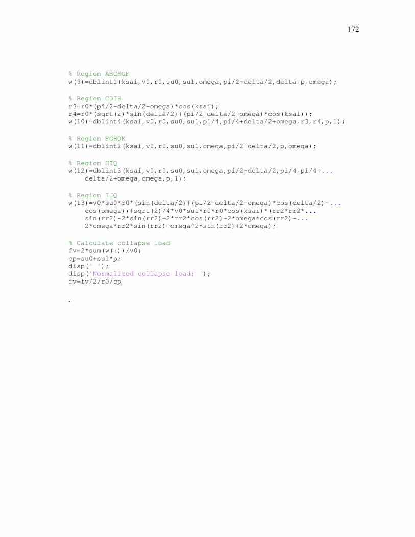
172

% Region ABCHGF w(9)=dblint1(ksai,v0,r0,su0,su1,omega,pi/2-delta/2,delta,p,omega); % Region CDIH r3=r0*(pi/2-delta/2-omega)*cos(ksai); r4=r0*(sqrt(2)*sin(delta/2)+(pi/2-delta/2-omega)*cos(ksai)); w(10)=dblint4(ksai,v0,r0,su0,su1,pi/4,pi/4+delta/2+omega,r3,r4,p,1); % Region FGHQK w(11)=dblint2(ksai,v0,r0,su0,su1,omega,pi/2-delta/2,p,omega); % Region HIQ w(12)=dblint3(ksai,v0,r0,su0,su1,omega,pi/2-delta/2,pi/4,pi/4+... delta/2+omega,omega,p,1); % Region IJQ w(13)=v0*su0*r0*(sin(delta/2)+(pi/2-delta/2-omega)*cos(delta/2)-... cos(omega))+sqrt(2)/4*v0*su1*r0*r0*cos(ksai)*(rr2*rr2*... sin(rr2)-2*sin(rr2)+2*rr2*cos(rr2)-2*omega*cos(rr2)-... 2*omega*rr2*sin(rr2)+omega^2*sin(rr2)+2*omega); % Calculate collapse load fv=2*sum(w(:))/v0; cp=su0+su1*p; disp(' '); disp('Normalized collapse load: '); fv=fv/2/r0/cp .

173

APPENDIX D

MATLAB PROGRAM: MINE_BURIAL

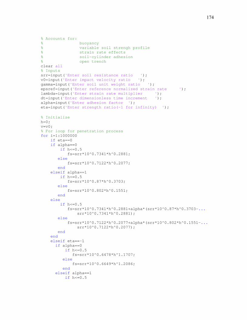
174

% Accounts for: % buoyancy % variable soil strengh profile % strain rate effects % soil-cylinder adhesion % open trench clear all % Inputs srr=input('Enter soil resistance ratio '); v0=input('Enter impact velocity ratio '); gamma=input('Enter soil unit weight ratio '); epsref=input('Enter reference normalized strain rate '); lambda=input('Enter strain rate multiplier '); dt=input('Enter dimensionless time increment '); alpha=input('Enter adhesion factor '); eta=input('Enter strength ratio(-1 for infinity) '); % Initialize h=0; v=v0; % For loop for penetration process for i=1:1000000 if eta==0 if alpha==0 if h<=0.5 fs=srr*10^0.7341*h^0.2881; else fs=srr*10^0.7122*h^0.2077; end elseif alpha==1 if h<=0.5 fs=srr*10^0.87*h^0.3703; else fs=srr*10^0.802*h^0.1551; end else if h<=0.5 fs=srr*10^0.7341*h^0.2881+alpha*(srr*10^0.87*h^0.3703-... srr*10^0.7341*h^0.2881); else fs=srr*10^0.7122*h^0.2077+alpha*(srr*10^0.802*h^0.1551-... srr*10^0.7122*h^0.2077); end end elseif eta==-1 if alpha==0 if h<=0.5 fs=srr*10^0.6478*h^1.1707; else fs=srr*10^0.6649*h^1.2086; end elseif alpha==1 if h<=0.5

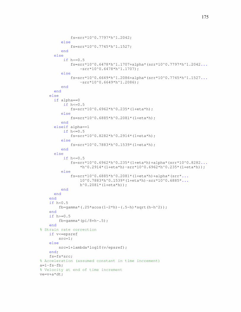
175

fs=srr*10^0.7797*h^1.2042; else fs=srr*10^0.7745*h^1.1527; end else if h<=0.5 fs=srr*10^0.6478*h^1.1707+alpha*(srr*10^0.7797*h^1.2042... -srr*10^0.6478*h^1.1707); else fs=srr*10^0.6649*h^1.2086+alpha*(srr*10^0.7745*h^1.1527... -srr*10^0.6649*h^1.2086); end end else if alpha==0 if h<=0.5 fs=srr*10^0.6962*h^0.235*(1+eta*h); else fs=srr*10^0.6885*h^0.2081*(1+eta*h); end elseif alpha==1 if h<=0.5 fs=srr*10^0.8282*h^0.2914*(1+eta*h); else fs=srr*10^0.7883*h^0.1539*(1+eta*h); end else if h<=0.5 fs=srr*10^0.6962*h^0.235*(1+eta*h)+alpha*(srr*10^0.8282... *h^0.2914*(1+eta*h)-srr*10^0.6962*h^0.235*(1+eta*h)); else fs=srr*10^0.6885*h^0.2081*(1+eta*h)+alpha*(srr*... 10^0.7883*h^0.1539*(1+eta*h)-srr*10^0.6885*... h^0.2081*(1+eta*h)); end end end if h<0.5 fb=gamma*(.25*acos(1-2*h)-(.5-h)*sqrt(h-h^2)); end if h>=0.5 fb=gamma*(pi/8+h-.5); end % Strain rate correction if v<=epsref src=1; else src=1+lambda*log10(v/epsref); end; fs=fs*src; % Acceleration (assumed constant in time increment) a=1-fs-fb; % Velocity at end of time increment ve=v+a*dt;

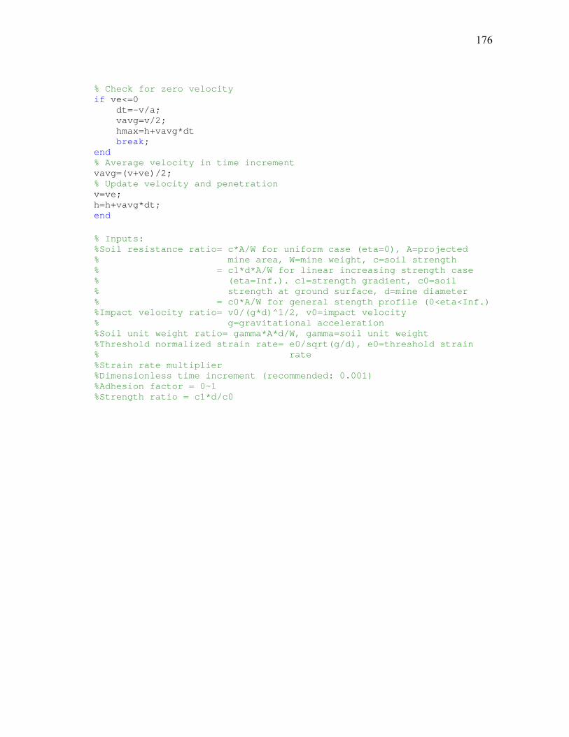
176

% Check for zero velocity if ve<=0 dt=-v/a; vavg=v/2; hmax=h+vavg*dt break; end % Average velocity in time increment vavg=(v+ve)/2; % Update velocity and penetration v=ve; h=h+vavg*dt; end % Inputs: %Soil resistance ratio= c*A/W for uniform case (eta=0), A=projected % mine area, W=mine weight, c=soil strength % = c1*d*A/W for linear increasing strength case % (eta=Inf.). c1=strength gradient, c0=soil % strength at ground surface, d=mine diameter % = c0*A/W for general stength profile (0<eta<Inf.) %Impact velocity ratio= v0/(g*d)^1/2, v0=impact velocity % g=gravitational acceleration %Soil unit weight ratio= gamma*A*d/W, gamma=soil unit weight %Threshold normalized strain rate= e0/sqrt(g/d), e0=threshold strain % rate %Strain rate multiplier %Dimensionless time increment (recommended: 0.001) %Adhesion factor = 0~1 %Strength ratio = c1*d/c0

177

APPENDIX E

MATLAB PROGRAM: XBP_SOFTCLAY

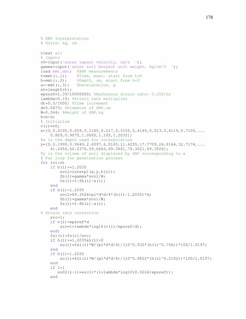
178

% XBP Interpretation % Units: kg, cm clear all % Inputs v0=input('enter impact velocity, cm/s '); gamma=input('enter soil buoyant unit weight, kg/cm^3 '); load mmt.dat; %XBP measurements t=mmt(:,1); %Time, msec, start from t=0 h=mmt(:,2); %Depth, cm, start from h=0 a=-mmt(:,3); %Deceleration, g nt=length(t); epsref=1.39/10000000; %Reference strain rate: 0.05%/hr lambda=0.15; %Strain rate multiplier dt=0.5/1000; %Time increment d=5.0673; %Diameter of XBP,cm W=0.544; %Weight of XBP,kg h=h/d; % Initialize v(1)=v0; x=[0,0.0195,0.059,0.1185,0.217,0.3155,0.4145,0.513,0.6115,0.7105,... 0.809,0.9075,1.0065,1.105,1.2035]; %x is the depth used for interpolation y=[0,0.1999,0.9649,2.6597,6.5165,11.6255,17.7709,24.8164,32.7174,... 41.2456,50.2374,59.6665,69.3861,79.3021,89.3526]; %y is the volume of soil displaced by XBP corresponding to x % For loop for penetration process for i=1:nt if h(i)<=1.2035 svol=interp1(x,y,h(i)); fb(i)=gamma*svol/W; fs(i)=1-fb(i)-a(i); end if h(i)>1.2035 svol=89.3526+pi*d*d/4*(h(i)-1.2035)*d; fb(i)=gamma*svol/W; fs(i)=1-fb(i)-a(i); end % Strain rate correction src=1; if v(i)>epsref*d src=1+lambda*log10(v(i)/epsref/d); end; fs1(i)=fs(i)/src; if h(i)<=1.2035&h(i)>0 su(i)=fs1(i)*W/(pi*d*d/4)/(10^0.932*(h(i)^0.756))*100/1.0197; end if h(i)>1.2035 su(i)=fs1(i)*W/(pi*d*d/4)/(10^0.9822*(h(i)^0.2102))*100/1.0197; end if i>1 su02(i-1)=su(i)*(1+lambda*log10(0.0224/epsref)); end

179

if i==nt break; else v(i+1)=v(i)+[a(i)+a(i+1)]/2*981*dt; end end h02=h(2:nt); plot(su02,h02*d); set(gca,'YDir','reverse'); ylabel('Depth (cm)','FontSize',12,'FontWeight','Demi'); xlabel ('Soil Strength (kPa)','FontSize',12,'FontWeight','Demi'); title('Soil Strength Profile','FontSize',14,'FontWeight','Demi');

180

APPENDIX F

A TYPICAL ABAQUS INPUT FILE (GENERATED BY ABAQUS CAE)

181

*Heading ** Job name: fr04 Model name: Model-1 *Preprint, echo=NO, model=NO, history=NO, contact=NO ** ** PARTS ** *Part, name=Part-1 *End Part ** ** ASSEMBLY ** *Assembly, name=Assembly ** *Instance, name=Part-1-1, part=Part-1 *Node 1, 0., -10. 2, 0., -100. 3, 100., -100. 6248, 3.895229, -12.94132 6249, 4.252222, -13.79167 6250, 4.176704, -13.55151 *Element, type=CPE4 1, 959, 742, 743, 960 2, 620, 619, 378, 379 3, 612, 627, 936, 626 6057, 6240, 5276, 5316, 5432 6058, 6243, 5782, 5760, 5637 6059, 6248, 6246, 5645, 5614 ** Region: (Section-1:Picked) *Elset, elset=_PickedSet2, internal, generate 1, 6059, 1 ** Section: Section-1 *Solid Section, elset=_PickedSet2, material=Material-1 1., *End Instance *Nset, nset=Set-1, instance=Part-1-1 1, 5, 6, 7, 8, 292, 293, 294, 295, 296, 297, 298, 299, 300, 301, 302 303, 304, 305, 306, 307, 308, 309, 310, 311, 312, 313, 314, 315, 316, 317, 318 319, 320, 321, 322, 323, 324, 325, 326, 327, 328, 329, 330, 331, 332, 333, 334 335, 336, 337, 338, 339, 340, 341, 342, 343, 344, 345, 346, 347, 348, 349, 350 351, 352, 353, 354, 355, 356, 357, 358, 359, 360, 361, 362, 363, 364, 365, 366 367, 368, 369, 370, 371, 372, 373, 374, 375, 376, 377, 378, 379, 380

182

*Elset, elset=Set-1, instance=Part-1-1 2, 4, 6, 7, 9, 10, 12, 14, 16, 17, 19, 21, 24, 25, 26, 31 38, 41, 43, 44, 228, 229, 233, 234, 235, 237, 242, 243, 246, 249, 250, 251 253, 257, 259, 261, 262, 263, 264, 265, 266, 267, 268, 270, 271, 272, 273, 279 280, 283, 285, 287, 289, 291, 292, 295, 296, 297, 300, 301, 303, 305, 306, 309 310, 312, 480, 482, 485, 490, 491, 492, 500, 502, 503, 529, 531, 533, 537, 539 541, 544, 547, 553, 557, 560, 563, 565, 567, 573, 585, 698, 811 *Nset, nset=_PickedSet5, internal, instance=Part-1-1 1, 2, 9, 10, 11, 12, 13, 14, 15, 16, 17, 18, 19, 20, 21, 22 23, 24, 25, 26, 27, 28, 29, 30, 31, 32, 33, 34, 35, 36, 37, 38 39, 40, 41, 42, 43, 44, 45, 46, 47, 48, 49, 50, 51, 52, 53, 54 55, 56, 57, 58, 59, 60, 61, 62, 63, 64, 65, 66, 67, 68, 69, 70 71, 72, 73, 74, 75, 76, 77, 78, 79, 80, 81, 82, 83, 84, 85, 86 87, 88, 89, 90, 91, 92, 93, 94, 95, 96, 97, 98, 99, 100, 101, 102 103, 104, 105, 106, 107, 108, 109, 110, 111, 112, 113, 114, 115, 116, 117, 118 119, 120, 121, 122, 123, 124, 125, 126, 127, 128, 129, 130, 131, 132, 133, 134 135, 136, 137, 138, 139, 140, 141, 142, 143, 144, 145, 146, 147, 148, 149, 150 151, 152, 153, 154, 155, 156, 157, 158, 159, 160, 161, 162, 163, 164, 165, 166 167, 168, 169, 170, 171 *Elset, elset=_PickedSet5, internal, instance=Part-1-1 5, 8, 18, 29, 30, 32, 35, 36, 37, 39, 40, 46, 47, 54, 58, 60 63, 64, 67, 68, 70, 71, 72, 73, 74, 75, 76, 78, 80, 81, 82, 83 84, 87, 90, 91, 93, 97, 108, 109, 110, 111, 112, 113, 114, 116, 118, 120 122, 123, 124, 130, 134, 151, 152, 155, 158, 159, 163, 184, 186, 187, 188, 197 201, 203, 204, 207, 208, 209, 211, 212, 213, 215, 216, 217, 219, 220, 221, 223 225, 269, 274, 276, 284, 288, 304, 305, 307, 308, 318, 333, 335, 337, 339, 341 343, 347, 349, 352, 353, 355, 359, 360, 364, 366, 367, 369, 371, 373, 375, 376 378, 379, 383, 384, 415, 421, 427, 428, 431, 436, 438, 439, 442, 453, 460, 463 468, 471, 543, 545, 548, 549, 551, 552, 554, 558, 559, 566, 569, 570, 571, 576 582, 587, 595, 597, 600, 604, 610, 615, 659, 670, 671, 697, 702, 703, 857, 862 866, 873, 906, 907 *Nset, nset=_PickedSet6, internal, instance=Part-1-1 3, 4, 205, 206, 207, 208, 209, 210, 211, 212, 213, 214, 215, 216, 217, 218 219, 220, 221, 222 *Elset, elset=_PickedSet6, internal, instance=Part-1-1 101, 103, 105, 173, 177, 179, 180, 182, 183, 192, 193, 322, 327, 403, 408, 424 623, 709, 1055 *Nset, nset=_PickedSet7, internal, instance=Part-1-1 2, 3, 172, 173, 174, 175, 176, 177, 178, 179, 180, 181, 182, 183, 184, 185 186, 187, 188, 189, 190, 191, 192, 193, 194, 195, 196, 197, 198, 199, 200, 201 202, 203, 204 *Elset, elset=_PickedSet7, internal, instance=Part-1-1 102, 125, 127, 129, 131, 136, 140, 141, 144, 145, 147, 149, 150, 152, 156, 161

183

162, 164, 165, 168, 174, 176, 178, 180, 181, 323, 324, 326, 368, 374, 382, 390 393, 405 *Nset, nset=_PickedSet8, internal, instance=Part-1-1 1, 5, 6, 7, 8, 292, 293, 294, 295, 296, 297, 298, 299, 300, 301, 302 303, 304, 305, 306, 307, 308, 309, 310, 311, 312, 313, 314, 315, 316, 317, 318 319, 320, 321, 322, 323, 324, 325, 326, 327, 328, 329, 330, 331, 332, 333, 334 335, 336, 337, 338, 339, 340, 341, 342, 343, 344, 345, 346, 347, 348, 349, 350 351, 352, 353, 354, 355, 356, 357, 358, 359, 360, 361, 362, 363, 364, 365, 366 367, 368, 369, 370, 371, 372, 373, 374, 375, 376, 377, 378, 379, 380 *Elset, elset=_PickedSet8, internal, instance=Part-1-1 2, 4, 6, 7, 9, 10, 12, 14, 16, 17, 19, 21, 24, 25, 26, 31 38, 41, 43, 44, 228, 229, 233, 234, 235, 237, 242, 243, 246, 249, 250, 251 253, 257, 259, 261, 262, 263, 264, 265, 266, 267, 268, 270, 271, 272, 273, 279 280, 283, 285, 287, 289, 291, 292, 295, 296, 297, 300, 301, 303, 305, 306, 309 310, 312, 480, 482, 485, 490, 491, 492, 500, 502, 503, 529, 531, 533, 537, 539 541, 544, 547, 553, 557, 560, 563, 565, 567, 573, 585, 698, 811 *End Assembly ** ** MATERIALS ** *Material, name=Material-1 *Elastic 5e+06, 0.499 *Plastic 400.,0. ** ** BOUNDARY CONDITIONS ** ** Name: BC-1 Type: Displacement/Rotation *Boundary _PickedSet5, 1, 1 ** Name: BC-2 Type: Displacement/Rotation *Boundary _PickedSet6, 1, 1 ** Name: BC-3 Type: Displacement/Rotation *Boundary _PickedSet7, 1, 1 _PickedSet7, 2, 2 ** ---------------------------------------------------------------- ** ** STEP: Step-1 ** *Step, name=Step-1 refined p/r=0.4

184

*Static 0.001, 1., 1e-05, 0.05 ** ** BOUNDARY CONDITIONS ** ** Name: BC-4 Type: Displacement/Rotation *Boundary _PickedSet8, 1, 1 _PickedSet8, 2, 2, -0.5 ** ** OUTPUT REQUESTS ** *Restart, write, frequency=1 ** ** FIELD OUTPUT: F-Output-1 ** *Output, field *Node Output, nset=Set-1 COORD, RF, U *Node Print, nset=Set-1 COORD, RF, U ** ** HISTORY OUTPUT: H-Output-1 ** *Output, history, variable=PRESELECT *El Print, freq=999999 *Node Print, freq=999999 *End Step

185

VITA

Han Shi was born on August 9, 1975 in Huanggang, China. He received his

Bachelor of Science degree in Hydrogeology & Engineering Geology from China

University of Geosciences, Wuhan in July 1995. He received his Master of Science

degree in Hydrogeology & Engineering Geology from China University of Geosciences,

Wuhan in June 1998. His permanent address is: 93 D3 District, 202, Huazhong

University of Science & Technology, Wuhan, Hubei 430074, China.