Embed Size (px)
Citation preview
Simulationen zur H− Charge ExchangeInjection in den CERN Proton Synchrotron
Booster mit Linac4
(Simulations of the H− Charge Exchange Injection into the CERN ProtonSynchrotron Booster with Linac4)
vonMatthias Scholz
geboren am10. August 1979
Diplomarbeit im Studiengang PhysikUniversität Hamburg
2010
1. Gutachter: Dr. Christan Carli2. Gutachter: Prof. Eckhart Elsen

Abstract
The CERN Proton Synchrotron Booster (PSB) is the first synchrotron of the LHC proton injectionchain. The main limitation of the Booster performance is given by direct space charge effects at low energy.Linac2, the present pre-accelerator of the Booster, will be replaced by Linac4 in 2015. The main motivationfor Linac4 is to increase the injection energy into the Booster from 50 MeV at present to 160 MeV tomitigate direct space charge effects. In addition, the conventional multiturn injection will be replaced byan H− charge exchange injection requiring special hardware and, in particular, a closed orbit bump inthe injection section (chicane) introducing perturbations on the lattice. Two different schemes which aimat mitigating the impact of these perturbations on PSB performance were tested: an active compensationwith additional quadrupole components at dedicated positions in the ring and a passive compensation withgradients added to the chicane magnets. To find the best setting for the injection, simulations with theparticle tracking code ORBIT were carried out for both schemes and the different results were compared.The simulations include the apertures, acceleration, space charge effects, scattering at the injection foil andplanned schemes to populate the available phase space in transverse and longitudinal plane (Painting).
Zusammenfassung
Der CERN Proton Synchrotron Booster (PSB) ist das erste Synchrotron in der LHC Protonen-Injektions-Kette. Die wichtigste Leistungseinschränkung ist durch direkte Raumladungskräfte bei niedrigen Energiengegeben. Linac2, der aktuelle Vorbeschleuniger des Boosters, wird im Jahr 2015 durch Linac4 ersetzt wer-den. Die Hauptmotivation für Linac4 ist die Erhöhung der Injektionsenergie in den Booster von derzeit 50MeV auf 160 MeV, um die direkten Raumladungseffekten abzuschwächen. Darüber hinaus wird die kon-ventionelle Multiturn-Injection durch eine H− Charge Exchange Injection ersetzt werden, welche spezielleBauteile erfordert, insbesondere einen closed Orbit Bump (Schikane) im Injektionsabschnitt, wodurchStörungen im Lattice verursacht werden. Zwei verschiedene Schemata zur Reduzierung der Auswirkun-gen dieser Störungen auf die Leistung des PSB wurden getestet: Eine aktive Kompensation mit zusätzlichenquadrupol Komponenten an geeigneten Positionen im Ring und eine passive Kompensation mit zusätzlichenGradienten in den Magneten der Schikane. Um die besten Einstellungen für die Injektionsschikane zufinden, wurden Simulationen für beide Schemata mit dem Particle Tracking Programm ORBIT ausgeführtund miteinander verglichen. Die Simulationen beinhalten die Aperturen, Beschleunigung, Raumladungsef-fekte, Streuung an der Injektionsfolie und geplante Schemata zur Füllung der bestehenden Phasenraumel-lipsen in transversaler und longitudinaler Ebene (Painting).

Contents
1 Introduction 11.1 Accelerators at CERN . . . . . . . . . . . . . . . . . . . . . . . . . . . . . . . . . . . . . 1
1.2 Linac4 project . . . . . . . . . . . . . . . . . . . . . . . . . . . . . . . . . . . . . . . . . 2
2 Theory 32.1 Transversal beam dynamics . . . . . . . . . . . . . . . . . . . . . . . . . . . . . . . . . . 4
2.1.1 Linear equation of motion . . . . . . . . . . . . . . . . . . . . . . . . . . . . . . 4
2.1.2 Transfer matrices . . . . . . . . . . . . . . . . . . . . . . . . . . . . . . . . . . . 5
2.1.3 Stability criterion for transfer matrices . . . . . . . . . . . . . . . . . . . . . . . . 6
2.1.4 Solution of the Hill equation . . . . . . . . . . . . . . . . . . . . . . . . . . . . . 7
2.1.5 Machine ellipse . . . . . . . . . . . . . . . . . . . . . . . . . . . . . . . . . . . . 8
2.1.6 Periodic dispersion . . . . . . . . . . . . . . . . . . . . . . . . . . . . . . . . . . 9
2.1.7 Edge focusing . . . . . . . . . . . . . . . . . . . . . . . . . . . . . . . . . . . . . 10
2.1.8 Horizontal painting . . . . . . . . . . . . . . . . . . . . . . . . . . . . . . . . . . 11
2.2 Longitudinal beam dynamics . . . . . . . . . . . . . . . . . . . . . . . . . . . . . . . . . 12
2.2.1 Acceleration and synchrotron movement . . . . . . . . . . . . . . . . . . . . . . 12
2.2.2 The physical emittance during acceleration . . . . . . . . . . . . . . . . . . . . . 14
2.2.3 Longitudinal painting . . . . . . . . . . . . . . . . . . . . . . . . . . . . . . . . . 15
2.3 Multiple scattering trough small angles . . . . . . . . . . . . . . . . . . . . . . . . . . . . 15
2.4 Direct space charge effects . . . . . . . . . . . . . . . . . . . . . . . . . . . . . . . . . . 16
2.5 Emittance calculations in the Booster measurement line . . . . . . . . . . . . . . . . . . . 19
3 The linear accelerators and the Proton Synchrotron Booster at CERN 213.1 Proton Synchrotron Booster . . . . . . . . . . . . . . . . . . . . . . . . . . . . . . . . . 21
3.1.1 Booster improvement programme . . . . . . . . . . . . . . . . . . . . . . . . . . 23
3.1.2 Variable tune . . . . . . . . . . . . . . . . . . . . . . . . . . . . . . . . . . . . . 24
3.2 PSB injection with Linac2 . . . . . . . . . . . . . . . . . . . . . . . . . . . . . . . . . . 24
3.2.1 Injection and ejection hardware . . . . . . . . . . . . . . . . . . . . . . . . . . . 25
3.2.2 Conventional multi turn injection . . . . . . . . . . . . . . . . . . . . . . . . . . 28
3.3 PSB injection with Linac4 . . . . . . . . . . . . . . . . . . . . . . . . . . . . . . . . . . 28
3.3.1 Injection to the 4 Booster rings . . . . . . . . . . . . . . . . . . . . . . . . . . . . 29
3.3.2 H− charge exchange injection . . . . . . . . . . . . . . . . . . . . . . . . . . . . 30
3.3.3 Active compensation . . . . . . . . . . . . . . . . . . . . . . . . . . . . . . . . . 32
3.3.4 Passive compensation . . . . . . . . . . . . . . . . . . . . . . . . . . . . . . . . 32
3.4 PS Booster measurement line . . . . . . . . . . . . . . . . . . . . . . . . . . . . . . . . . 33
iii
4 Measurements 354.1 Beam properties . . . . . . . . . . . . . . . . . . . . . . . . . . . . . . . . . . . . . . . . 354.2 PSB sensitivity to variations of compensation . . . . . . . . . . . . . . . . . . . . . . . . 374.3 Dynamic working point of the PS Booster . . . . . . . . . . . . . . . . . . . . . . . . . . 40
5 ORBIT Simulations 435.1 About ORBIT simulations . . . . . . . . . . . . . . . . . . . . . . . . . . . . . . . . . . 435.2 Particle distribution for injection . . . . . . . . . . . . . . . . . . . . . . . . . . . . . . . 455.3 Simulations . . . . . . . . . . . . . . . . . . . . . . . . . . . . . . . . . . . . . . . . . . 45
5.3.1 Implementation of the acceleration . . . . . . . . . . . . . . . . . . . . . . . . . . 455.3.2 Implementation of the apertures . . . . . . . . . . . . . . . . . . . . . . . . . . . 465.3.3 Benchmarking on the number of macro particles . . . . . . . . . . . . . . . . . . 505.3.4 Different scattering models for the injection foil . . . . . . . . . . . . . . . . . . . 515.3.5 Impact of the foil implementation method . . . . . . . . . . . . . . . . . . . . . . 535.3.6 Quadrupole resonances . . . . . . . . . . . . . . . . . . . . . . . . . . . . . . . . 535.3.7 Passive compensation with different pole face rotations . . . . . . . . . . . . . . . 555.3.8 Comparison of active and passive compensation . . . . . . . . . . . . . . . . . . . 595.3.9 Imperfect active compensation . . . . . . . . . . . . . . . . . . . . . . . . . . . . 62
6 Conclusions and prospects 65
A Deviations due to the re-installation of the lattice 67
B Measurements at the PS Booster 69
C Simulation settings 71
Chapter 1
Introduction
This thesis was written at the BE department at the CERN laboratory. CERN is the largest particle physicslaboratory in the world, situated in the northwest suburbs of Geneva [1]. The thesis is concerned with theinjection from a linac to a synchrotron and it was the task to run simulations to assess the feasibility of futuremachines and components. To this end, the particle tracking programme ORBIT [2] had to be understoodas far as it was necessary to run simulations. This was realised step by step in such a way, that the simulatedelements like apertures and injection equipment were added to the runs one by one. At the end, severalsimulations were carried out to compare different injection schemes investigating if they are feasible for therequired beam parameters and, in case that they work, to explore which one provides the best results.
1.1 Accelerators at CERN
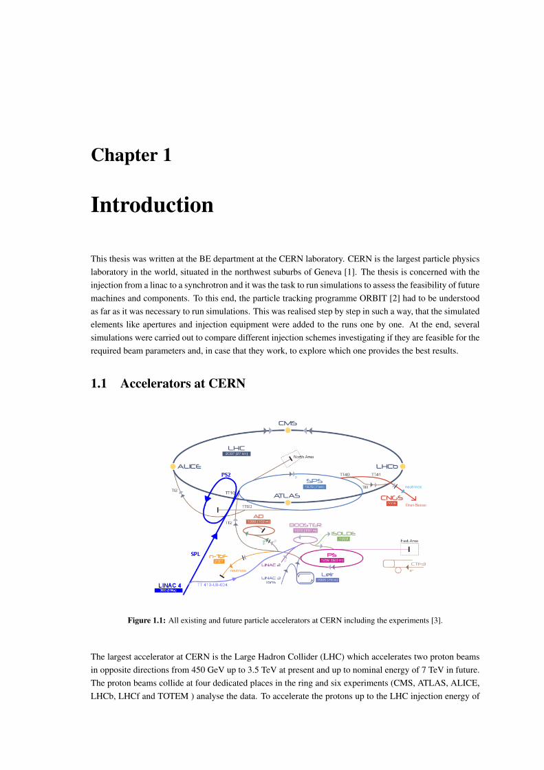
Figure 1.1: All existing and future particle accelerators at CERN including the experiments [3].
The largest accelerator at CERN is the Large Hadron Collider (LHC) which accelerates two proton beamsin opposite directions from 450 GeV up to 3.5 TeV at present and up to nominal energy of 7 TeV in future.The proton beams collide at four dedicated places in the ring and six experiments (CMS, ATLAS, ALICE,LHCb, LHCf and TOTEM ) analyse the data. To accelerate the protons up to the LHC injection energy of
2 LINAC4 PROJECT
450 GeV, a chain of pre-accelerators, starting with a linac and followed by three synchrotrons, is in use.At present, the first machine after the proton source is the Linac2 which accelerates the particles up to anenergy of 50 MeV. The first synchrotron is the Proton Synchrotron Booster (PSB) with an ejection energyof 1.4 GeV, followed by the Proton Synchrotron (PS) where the particles get accelerated up to 26 GeV. Thelast synchrotron in the LHC injector chain is the Super Proton Synchrotron (SPS) which provides particleenergies up 450 GeV for the LHC injection. Beside the proton acceleration, the LHC can also acceleratelead ions up to a maximum energy of 2.67 TeV per nucleon. The pre-accelerator chain for the ions consistof Linac3, LEIR, the PS and finally the SPS from where the injection to the LHC takes place. There are alsomore experiments than those around the LHC like the Antiproton Decelerator (AD), positioned behind thePS, the Isotope Separator On-Line (ISOLDE) experiment which is supplied with protons by the PS Boosteror the CERN Neutrinos for Gran Sasso (CNGS) experiment, receiving protons from the SPS. The proposedfuture accelerators Linac4, SPL (Superconducting Proton Linac) and PS2 are shown in Fig. 1.1 on the lefthand side in blue color.
1.2 Linac4 project
Linac4 will replace Linac2 in 2015 and the H− ions accelerated with Linac4 will be injected to the PSBooster whose main limitations are direct space charge effects at low energies. The higher injection energyof 160 MeV instead of 50 MeV with Linac2 will mitigate the direct space charge effects and allow increasingthe beam intensity and brightness of the Booster. To this end, the conventional multi turn injection used withLinac2 has to be replaced by a charge exchange injection where the ions will be stripped to protons by a thincarbon foil. The charge exchange injection requires two closed orbit bumps, the so-called "chicane" and the"injection painting" bump, both consisting out of four magnets. All injection elements have to be within thespace available in the fixed lattice of the existing Booster. These constrains lead to short chicane magnetsinstalled in the short injection straight section with a deflection angle of 66 mrad introducing additionalvertical focusing effects perturbing the lattice. The perturbations will induce strong beta beating since thevertical tune is close to a half integer resonance. To compensate the perturbations, two different methodswere tested, the "passive" and the "active" compensation scheme. For the first scheme, additional gradientshave to be added to the chicane’s magnets which have the same effect on the beam than rotations of themagnet’s pole faces reducing the focusing effects and the strong beta beating in vertical plane. However,using this compensation scheme, one induces perturbations in the horizontal plane, but the consequencesare less due to the fact that the beam is not close to a half-integer resonance in this plane. The secondpossibility to compensate the perturbations is to install additional quadrupole components to defocusingmagnets existing in the lattice at dedicated positions outside the injection area. The positions have to bechosen such that the betatron phase advance between the perturbations and the compensation are suitable.These constrains are fulfilled by the defocusing magnets in the Booster periods 3 and 14.To accumulate the particles for a high intensity beam with 1.6×10¹³ protons in the Booster, one has to injectthe particles over 100 turns. For injections over several turns, one can apply so-called "painting-schemes"in order to fill the available phase in transversal and longitudinal plane with an even density distribution. Tothis end, the second closed orbit bump, the "painting bump", will be superimposed with the chicane in thecharge exchange injection section allowing to use the painting scheme in horizontal plane. The longitudinalpainting will be realised by varying energy of the Linac4 in a controlled way.The aim of this thesis was to study different injection and compensation schemes and to compare them inorder to provide information required to take the decision which compensation scheme should be used andhow the injection from the Linac4 to the Booster could be managed.

Chapter 2
Theory
This chapter will tread all topics about accelerator physics which are applied in this thesis from the the-oretical point of view. To avoid mistakes due to not clearly declared signs, Tab. 2.1 shows all used signsincluding the declarations.
Table 2.1: Declaration of the used signs.
α The related Twiss-function v Velocityβ The related Twiss-function ε∗x Normalised horizontal rms Emittanceγ The related Twiss-function εx Physical horizontal rms Emittancec Speed of Light ε∗y Normalised vertical rms Emittanceβrel Velocity/c εy Physical vertical rms Emittanceγrel The Lorentz factor k Focusing strengthm0 Rest mass B Magnetic fluxe Elementary charge D Dispersionp Momentum U Circumference
Furthermore, the coordinate System, as shown in Fig. 2.1, was used for the calculations and descriptions.
~ex(s1)
~ey(s1)
~ez(s1)
~ex(s2)
~ey(s2)
x(s1)
y(s1)O s s1
s2
ρ(s1)
~r(s1)
Figure 2.1: The machine coordinate system used in this thesis. ~ex(s), ~ey(s) and ~ez(s) describe a local coordinatesystem at the longitudinal position s in the lattice.
The particle positions can be described in this coordinate system with vectors:
~r(s) = ~r0(s) + x(s) ~ex(s) + y(s) ~ey(s) (2.1)
4 TRANSVERSAL BEAM DYNAMICS
2.1 Transversal beam dynamics
2.1.1 Linear equation of motion
The linear equation of motion for both transversal planes for particles circulating the machine can be writtenas [4]:
x′′ +K x =1
ρx
∆p
p0(2.2)
y′′ + k y = 0. (2.3)
With the magnetic field gradient k and K =(
1ρ2 + k
)and the derivatives x′′ = d2x
ds2 and y′′ = d2yds2 .
The general solution x(s) of the Eq. 2.2 is the sum of the solution xh of the homogeneous equation (likeEq. 2.3) and a particular solution xi of the inhomogeneous equation.
x(s) = xh(s) + xi(s) (2.4)
with:
x′′h(s) +K xh(s) = 0 (2.5)
x′′i (s) +K xi(s) =1
ρx(s)
∆p
p0. (2.6)
To separate the particle properties from the machine properties, one can write the solutions of the inhomo-geneous equation like:
D(s) =xi
∆p/p0. (2.7)
The general solution is then
x(s) = C(s)x0 + S(s)x′0 +D(s)∆p
p0, (2.8)
with the cosine and sine like functions C(s) and S(s) plus the initial values x(s0) = x0 and x′(s0) = x′0.The principal solutions of homogeneous differential equation are [5]:
C(s) = cos√Ks and S(s) =
1√K
sin√Ks for K > 0 (2.9)
and
C(s) = cosh√|K|s and S(s) =
1√|K|
sinh√|K|s for K < 0. (2.10)
In order to proof the independence of these solutions, one can calculate the Wronski determinant W:
W =
∣∣∣∣∣C S
C ′ S′
∣∣∣∣∣ = CS′ − SC ′ = C2 + S2 = 1 6= 0. (2.11)
The non-zero Wronski determinant verifies the independence of the two solutions of the homogeneousequation. To investigate the developing of the determinant, one can calculate its derivative with respect tothe longitudinal coordinate s:
2.1.2 Transfer matrices 5
d
ds(CS′ − SC ′) = CS′′ − SC ′′ = K (CS − SC) = 0. (2.12)
The derivative of the Wronski determinant vanishes which means, the value of the determinant will notchange: W (s) = W (s0). For this reason, the independence between the two solutions is preserved.
The solution of the inhomogeneous equation was defined as:
D(s) =xi
∆p/p0. (2.13)
The Dispersion D(s) describes the part of the motion which is depending on the momentum. x(s) and x’(s)are related to their initial values by a linear transformation. Taking also the longitudinal component intoaccount, one can write:
x(s) = C x0 + S x′0 +D
(∆p
p0
)0
(2.14)
x′(s) = C ′ x0 + S′ x′0 +D′(
∆p
p0
)0
. (2.15)
The Dispersion can be calculated by:
D(s) = S(s)
s∫so
1
ρ(t)C(t) dt− C(s)
s∫s0
1
ρ(t)S(t) dt. (2.16)
This definition fulfils the inhomogeneous part of Eq. 2.2 [6].
2.1.2 Transfer matrices
Transfer matrices describe the particle movement between two positions of the lattice [4]. A transfer matrixcan be allocated to each element in the ring as well as to sets of elements. If the initial particle coordinatesand the transfer matrices are known, the coordinates at all other positions in the lattice can be calculated by:
~r(s) = M0,s ~r0. (2.17)
The matrices for several elements can be calculated multiplying the matrices of the single elements
Mset =∏i
Mi. (2.18)
Furthermore, the general transfer matrix is related to the sine and cosine like solutions of the linear equationof motion as well as to the dispersion. It is possible to write transfer matrices just for one plane, for thetransversal planes or for all planes of the six-dimensional phase space, whereas the last two options allowalso to implement the impacts between the planes. Below, there will be presented exemplary transfer ma-trices for different lattice elements.
The transfer matrix for a drift with length L is:
DS =
1 L 0 0 0 0
0 1 0 0 0 0
0 0 1 L 0 0
0 0 0 1 0 0
0 0 0 0 1 Lγ2rel
0 0 0 0 0 1
. (2.19)
6 TRANSVERSAL BEAM DYNAMICS
The transfer matrices for a focusing and a defocusing quadrupole magnet with lengthL, maximum magneticfield B0 and aperture a are:
QF =
cos√kL sin
√kL√k
0 0 0 0
−√k sin
√kL cos
√kL 0 0 0 0
0 0 cosh√kL sinh
√kL√k
0 0
0 0√k sinh
√kL cosh
√kL 0 0
0 0 0 0 1 Lγ2rel
0 0 0 0 0 1
, (2.20)
QD =
cosh√kL sinh
√kL√k
0 0 0 0√k sinh
√kL cosh
√kL 0 0 0 0
0 0 cos√kL sin
√kL√k
0 0
0 0 −√k sin
√kL cos
√kL 0 0
0 0 0 0 1 Lγ2rel
0 0 0 0 0 1
. (2.21)
As an example for a matrix with interactions between the phase spaces of the different planes, the followingmatrix shows the transfer matrix for a sector bend with bending radius ρ0, deflection angle α and the lengthL:
SB =
cosα ρ0 sinα 0 0 0 ρ0(1− cosα)
− sinαρ0
cosα 0 0 0 sinα
0 0 1 ρ0α 0 0
0 0 0 1 0 0
− sinα −ρ0(1− cosα) 0 0 1 ρ0αγ2rel− ρ0(α− sinα)
0 0 0 0 0 1
. (2.22)
2.1.3 Stability criterion for transfer matrices
To get the transfer matrix Mcirc for a complete turn, one has to multiply all single matrices of the latticeelements (cf. Eq. 2.18). To calculate the transfer matrix for n turns, one has to apply Mcirc for n times:
Mn = (Mcirc)n. (2.23)
It is important to find out if there are constrains on the transfer matrices in order to run the machine stable.To get more information about the impact of a transfer matrix on the stability, one can investigate theeigenvalues of the matrix.
M ~x = λ ~x with ~x =
(x
x′
)(2.24)
Using Tr(M) = 2 cosµ, one calculates:

2.1.4 Solution of the Hill equation 7
λ1/2 = exp±iµ. (2.25)
Excluding the case Tr(M) = 2, the matrix M can be expressed in a useful form applying the Twiss matrix:
M = I cosµ+ J sinµ with I =
(1 0
0 1
), J =
(α β
−γ −α
). (2.26)
With the Twiss parameters α, β and γ calculated with the elements mij of the matrix M:
α =m11 −m22
2 sinµ, β =
m12
sinµ, γ = −m21
sinµ. (2.27)
The transfer matrix for n turns is then:
Mn = I cosnµ+ J sinnµ. (2.28)
For real µ, the elements of the matrix Mn oscillate but remain bounded for any n. But, for complex orimaginary µ, cosµ and sinµ will increase exponentially and the motion becomes unbounded [6]. Thisleads to the following constrains for the transfer matrices:
Tr(M) < 2. (2.29)
2.1.4 Solution of the Hill equation
To describe the Twiss parameters, one has to find the solution of the Hill equation [4,6]:
x′′(s) + k(s) x(s) = 0, (2.30)
with the periodicity k(s+ U) = k(s) and the circumference of the machine U .
Floquet’s theorem assures two linearly independent solutions of the Hill equation which are:
xm(s+ U) = xm(s) exp±iµ (2.31)
= xm(s) (cosµ± i sinµ), m = 1, 2. (2.32)
The solutions xm(s+ U) and xm(s) are also correlated with the Twiss matrix:(xm(s+ U)
x′m(s+ U)
)=
(cosµ+ α sinµ β sinµ
−γ sinµ cosµ− sinµ
)(xm(s)
x′m(s)
)(2.33)
For x(s), this can also be written as:
x(s) (cosµ± i sinµ) = (cosµ+ α sinµ) xm(s) + β sinµ x′m(s). (2.34)
Using Eq. 2.34 and the Hill equation, one can derive the following differential equation for β:
1
2ββ′′ − 1
4β′ + kβ2 = 1. (2.35)
This equation shows the correlation between the Twiss parameter β and the focusing strength k. For con-stant k, one can calculate that β = 1/
√k. The beta function β(s) can be derived by solving Eq.2.35
numerically, but in most cases it will be derived from the transfer matrices for one turn. The other Twissparameters are given by:
8 TRANSVERSAL BEAM DYNAMICS
α = −1
2β′, γ =
1 + α2
β. (2.36)
The independent solutions proposed by Floquet’s theorem are:
xm(s) = am√β exp±ψ(s) with ψ =
s∫0
1
β(t)dt, m = 1, 2. (2.37)
The general solution can be written as the linear combination of the two independent solutions
x(s) = a1√β(s) exp [iψ(s)] + a2
√β(s) exp [−iψ(s)], (2.38)
and the particle trajectory is described by a real solution:
x(s) = a√β(s) cosψ(s) + ψ0). (2.39)
The variables a and ψ0 define the individual trajectory of the particle. Eq. 2.39 describes a quasi harmonicoscillation with variable amplitude a
√β(s) and variable wave number dψ/ds = 1/β(s). The number of
oscillations per turn, known as the tune of the machine, is:
Qx,y =1
2π
s+U∫s
dt
βx,y(t). (2.40)
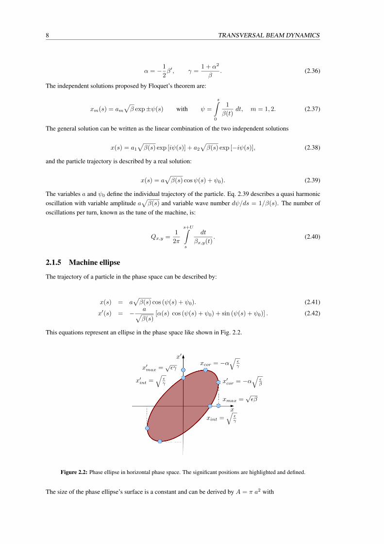
2.1.5 Machine ellipse
The trajectory of a particle in the phase space can be described by:
x(s) = a√β(s) cos (ψ(s) + ψ0). (2.41)
x′(s) = − a√β(s)
[α(s) cos (ψ(s) + ψ0) + sin (ψ(s) + ψ0)] . (2.42)
This equations represent an ellipse in the phase space like shown in Fig. 2.2.
xmax =√εβ
xint =√
εγ
x
x′cor = −α√
εβ
xcor = −α√
εγ
x′
x′max =√εγ
x′int =√
εγ
Figure 2.2: Phase ellipse in horizontal phase space. The significant positions are highlighted and defined.
The size of the phase ellipse’s surface is a constant and can be derived by A = π a2 with
2.1.6 Periodic dispersion 9
γx2 + 2αxx′ + βx′2 = a2 (2.43)
which is the Courant-Snyder invariant. The maximum amplitudes in x and x′ direction are given by
xmax =√εβ and x′max =
√εγ (2.44)
using the emittance ε = a2. The physical interpretation of the Courant-Snyder invariant corresponds to [4]:
• A particle with the coordinates (x, x′) moves in the phase space on the edge of an ellipse whose formis related to the particles’ position in the lattice.
• The size of the ellipse’s surface area defining the particles’ movement is constant and given by theparticles’ amplitudes.
• The form of the ellipse is given by the lattice and can be displayed using the Twiss parameters α, βand γ.
• The phase ellipse defined by the Courant-Snyder invariant a2 = ε describes the movement in phasespace for all particles with betatron amplitudes smaller or equal to a.
2.1.6 Periodic dispersion
The periodic dispersion of the lattice is described by the differential equation [4]:
x′′ + kx(s) x =1
ρ0
∆p
p0, (2.45)
with the coefficients kx(s + U) = kx(s) and ρ0(s + U) = ρ0(s) whereas U is the circumference ofthe machine or the length of a super period of the lattice. Due to the relative momentum offset ∆p/p0,the particles will circulate the machine with an additional offset xD compared to the closed orbit withoutmomentum deviation.
xD(s) = D(s)∆p
p0. (2.46)
The modified orbit is, like the orbit for particles with ∆p/p0 = 0, a periodic solution and D(s) is theperiodic dispersion of the lattice. The general solution of Eq. 2.45 is:
x(s) = xD(s) + xβ(s). (2.47)
with xD(s), the offset caused by the dispersion, and xβ(s), the offset due to betatron oscillations.Inserting Eq. 2.47 to Eq. 2.45, one can derive a differential equation for the dispersion:
D′′ + k(s) D =1
ρ(s)(2.48)
whose solution has to fulfill the periodicity conditions of the dispersion:
D(s+ U) = D(s) (2.49)
D(s+ U) = D(s). (2.50)
To solve this differential equation, one has to chose a fixed starting point s0 = 0 with D0 and D′0. Thesolutions at the position s is then identical with:
10 TRANSVERSAL BEAM DYNAMICS
D(s) = D0 C(s) +D′0 S(s) + d(s). (2.51)
In this connection, d(s) is a special solution depending on the periodicity conditions and C(s) respectivelyS(s) are the cosine and sine like solutions of the homogeneous equation (cf. section 2.1.1). ComparingD(s) with D(s + U) and taking the periodicity conditions into account, one can derive the dispersionfunction:
D(s) =
√β(s)
2 sin(µ2
) s+C∫s
1
ρ(t)
√β(t) cos
(ψ(t)− ψ(s)− µ
2
)dt with µ =
s+U∫s
dt
β(t). (2.52)
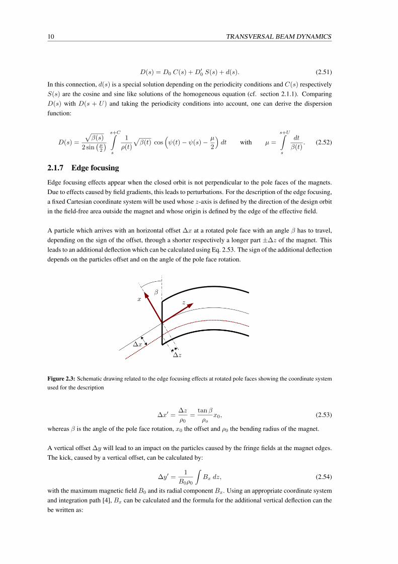
2.1.7 Edge focusing
Edge focusing effects appear when the closed orbit is not perpendicular to the pole faces of the magnets.Due to effects caused by field gradients, this leads to perturbations. For the description of the edge focusing,a fixed Cartesian coordinate system will be used whose z-axis is defined by the direction of the design orbitin the field-free area outside the magnet and whose origin is defined by the edge of the effective field.
A particle which arrives with an horizontal offset ∆x at a rotated pole face with an angle β has to travel,depending on the sign of the offset, through a shorter respectively a longer part ±∆z of the magnet. Thisleads to an additional deflection which can be calculated using Eq. 2.53. The sign of the additional deflectiondepends on the particles offset and on the angle of the pole face rotation.
β
∆z
∆x
xz
Figure 2.3: Schematic drawing related to the edge focusing effects at rotated pole faces showing the coordinate systemused for the description
∆x′ =∆z
ρ0=
tanβ
ρox0, (2.53)
whereas β is the angle of the pole face rotation, x0 the offset and ρ0 the bending radius of the magnet.
A vertical offset ∆y will lead to an impact on the particles caused by the fringe fields at the magnet edges.The kick, caused by a vertical offset, can be calculated by:
∆y′ =1
B0ρ0
∫Bx dz, (2.54)
with the maximum magnetic field B0 and its radial component Bx. Using an appropriate coordinate systemand integration path [4], Bx can be calculated and the formula for the additional vertical deflection can thebe written as:
2.1.8 Horizontal painting 11
∆y′ = −y0tanβ
ρ0. (2.55)
The transfer matrix for edge focusing can then be expressed as:
EF =
1 0 0 0 0 0tan βρ0
1 0 0 0 0
0 0 1 0 0 0
0 0 − tan βρ0
1 0 0
0 0 0 0 1 0
0 0 0 0 0 1
. (2.56)
2.1.8 Horizontal painting
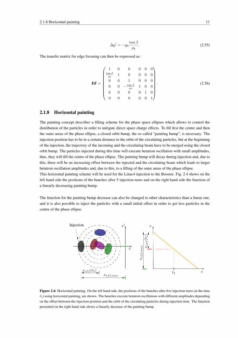
The painting concept describes a filling scheme for the phase space ellipses which allows to control thedistribution of the particles in order to mitigate direct space charge effects. To fill first the centre and thenthe outer areas of the phase ellipse, a closed orbit bump, the so called "painting bump", is necessary. Theinjection position has to be in a certain distance to the orbit of the circulating particles, but at the beginningof the injection, the trajectory of the incoming and the circulating beam have to be merged using the closedorbit bump. The particles injected during this time will execute betatron oscillation with small amplitudes,thus, they will fill the centre of the phase ellipse. The painting bump will decay during injection and, due tothis, there will be an increasing offset between the injected and the circulating beam which leads to largerbetatron oscillation amplitudes and, due to this, to a filling of the outer areas of the phase ellipse.This horizontal painting scheme will be used for the Linac4 injection to the Booster. Fig. 2.4 shows on theleft hand side the positions of the bunches after 5 injection turns and on the right hand side the function ofa linearly decreasing painting bump.
The function for the painting bump decrease can also be changed to other characteristics than a linear one,and it is also possible to inject the particles with a small initial offset in order to get less particles in thecentre of the phase ellipse.
xoff,max
xoff (t5)t5
xoff(t
5)
xoff,max
x
x′ x
t
Injection
Figure 2.4: Horizontal painting. On the left hand side, the positions of the bunches after five injection turns (at the timet5) using horizontal painting, are shown. The bunches execute betatron oscillations with different amplitudes dependingon the offset between the injection position and the orbit of the circulating particles during injection time. The functionpresented on the right hand side shows a linearly decrease of the painting bump.
12 LONGITUDINAL BEAM DYNAMICS
2.2 Longitudinal beam dynamics
This section will be concerned with the longitudinal beam dynamics as observed in a synchrotron withRF acceleration cavities. The acceleration and the synchrotron oscillations will be discussed and a fillingscheme for the buckets, the longitudinal painting as used for the Linac4 injection, will be presented as well.
2.2.1 Acceleration and synchrotron movement
To accelerate particles in a synchrotron using a radio frequency field, the following condition between therotational frequency of the particles ωs and the accelerating radio frequency ωRF has to be fulfilled:
ωHF = h ωs. (2.57)
The harmonic number h has to be an integer value in order to allow constant acceleration during the cycle.The rotational frequencies in the Booster during injection with 160 MeV and ejection with 1.4 GeV are:
ωs, 160 MeV = 6.23× 1061
sand ωs, 1.4 GeV = 10.98× 10⁶
1
s. (2.58)
As the main harmonic number h = 1 is used in the Booster (cf. section 3.1), these numbers are the samefor the RF-frequency ωRF for the respective particle energies.Passing the acceleration cavities, the particles will gain a certain amount of energy which is related to thepeak voltage of the RF U0 and to the synchrotron phase φ which describes the relative position of theparticle in comparison to the sine like RF wave:
∆E = q U0 sinφ. (2.59)
A particle which has a certain phase φ = φs is called the synchronous particle. This particle will passthe RF wave at each turn at exactly the same position and will gain the same energy every time. In eachperiod of the RF, one can find two positions with the same voltage, one at the flank with positive and theother on the flank with negative slope, which means, that there are two positions where the particles withφ = φs could be accelerated. More about the decision which slope of the RF has to be chosen – it dependson the behavior of the particles with φ 6= φs – will be presented below. Assuming that the particles withhigher energy than the synchronous particle accomplish one circulation in less time and arrive earlier atthe cavity, i.e. they have a phase with φ > φs, then, the position of φs has to be chosen at the decreasingslope of the RF wave in order to accelerate particles with higher energy less and particles with lower energymore than the synchronous particle. Due to this, particles will carry out longitudinal oscillations around thesynchronous phase φs which are called the synchrotron oscillations. For those oscillations, it is essentialthat the angular frequency ω is related to the momentum p of the particles:
∆ω
ω=
(1
γ2rel− 1
γ2tr
)∆p
p0. (2.60)
Eq. 2.60 shows that the relative frequency deviation ∆ω is related on the particles energy. Particles withan energy below the so called transition energy Etr = γtr E0 and with an positive momentum offset willcirculate the machine in a shorter time than particles with the same energy and a negative momentum offset.This is the other way around for particles with an Energy above Etr. The velocity of the particles with anenergy below transition energy is still far away enough from the speed of light that means the velocity ofthese particles is increased significantly passing an acceleration cavity. Due to this, the particles with anpositive momentum offset need less time for one turn than the particles with smaller or negative momentumoffsets. The second effect, which is dominant for particle energies above the transition energy, is thatparticles with positive momentum offset will be bend on a larger radius than those with negative ∆p/p0.
2.2.1 Acceleration and synchrotron movement 13
This leads to a larger circumference and, as a result, to longer circulation times. The threshold value forthe particle energy between the dominance of the two effects is the transition energy. Eq. 2.60 shows alsothat there will be no synchrotron movement and, due to this, no longitudinal focusing for γrel = γtr. Forthis reason, the particles have to cross the transition energy during acceleration as fast as possible in orderto avoid a divergence of the bunch. γtr is related to the momentum compaction factor:
αP =1
γ2tr=
∮U
D(s)
ρds (2.61)
with the dispersion D(s), the bending radius of the machine ρ and the machine circumference U .
For the calculations of the synchrotron oscillations, the particle movement will be described relative to thesynchronous particle, using
∆φ = φ− φs, ∆p = p− ps, ∆E = E − Es, ∆ω = ω − ωs. (2.62)
For the variations of ∆φ and ∆E, one can calculate [4]:
δ(∆φ) = −ηs∆p
psh 2π (2.63)
δ(∆E) = qU0(sinφ− sinφs). (2.64)
Divide this equations by the cycle period Ts = 2π/ωs:
d
dt∆φ = − 1
Tsηs
∆p
psh 2π = −hηsωs
psvs∆E (2.65)
d
dt∆E =
1
TsqU0(sinφ− sinφs) =
ωs2πqU0(sinφ− sinφs). (2.66)
The variables ηs, ωs, ps, U0 and φs vary hardly and will be used as constants in order to simplify the calcu-lation.
An additional differentiation d/dt applied on Eq. 2.65 gives the possibility to insert Eq. 2.66 and to combineboth equations to one:
d2
dt2∆φ = −hηsωs
psvs
d
dt∆E (2.67)
= − hηsω2s
2πpsvsqUo(sinφ− sinφs). (2.68)
Applying a linear approximation on sinφ − sinφs, valid for small φ, using sinφ = φ and cosφ = 1, onegets:
sinφ− sinφs ≈ cos (φ)∆φ. (2.69)
Inserting this approximations to Eq. 2.68, one gets a differential equation for a harmonic oscillator:
d2
dt2∆φ+ Ω2 ∆φ = 0 with Ω =
√hηsω2
s
2πpsvsqUo cosφs. (2.70)
The particles will carry out synchrotron oscillations with the frequency fsyn = Ω/2π if Ω is real. Thecondition for a real Ω is η cosφs > 0. Furthermore, one calculates the longitudinal tune with:
14 LONGITUDINAL BEAM DYNAMICS
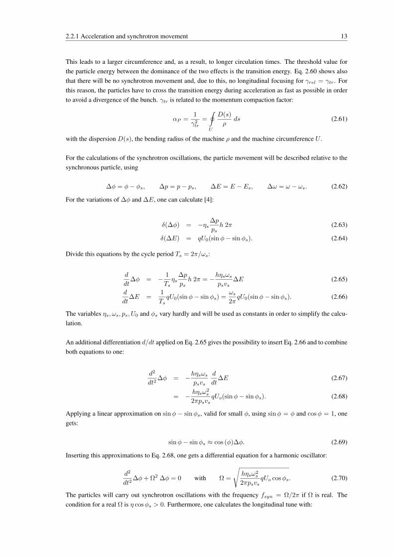
Figure 2.5: The upper plot shows the sine like RF wave and the lower plot the separatrix of the bucket which dividesthe areas for stable and unstable oscillation in the longitudinal phase space. The phase for the synchronous particle islabelled with φs.
Qsyn =Ω
ω=
√hηs
2πpsvsqUo cosφs. (2.71)
Using ∆φ = ∆φ0 cos (Ωt) as a solution of an harmonic oscillator and inserting to Eq. 2.65, one gets:
∆E = ∆E0 sin Ωt with ∆E0 =Ω
ωs
psvshηs
∆φ0. (2.72)
The solution of the harmonic oscillator ∆φ = ∆φ0 cos (Ωt) and Eq. 2.72 build a parametric equation of anellipse as presented in Fig. 2.5. The synchrotron oscillation is a coupled oscillation in the (∆φ,∆E)-planeand the amplitudes are depending on each other in the way as shown in Eq. 2.73 [4].
∆E0 = Qsynpsvshηs
∆φ0. (2.73)
2.2.2 The physical emittance during acceleration
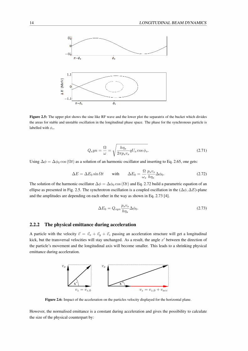
A particle with the velocity ~v = ~vx + ~vy + ~vz passing an acceleration structure will get a longitudinalkick, but the transversal velocities will stay unchanged. As a result, the angle x′ between the direction ofthe particle’s movement and the longitudinal axis will become smaller. This leads to a shrinking physicalemittance during acceleration.
vx vx
vz = vz,0 vz = vz,0 + vacc
x’ x’
Figure 2.6: Impact of the acceleration on the particles velocity displayed for the horizontal plane.
However, the normalised emittance is a constant during acceleration and gives the possibility to calculatethe size of the physical counterpart by:
2.2.3 Longitudinal painting 15
ε =ε∗
βrelγrel. (2.74)
2.2.3 Longitudinal painting
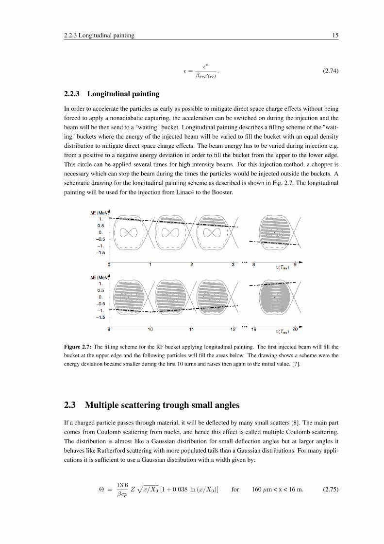
In order to accelerate the particles as early as possible to mitigate direct space charge effects without beingforced to apply a nonadiabatic capturing, the acceleration can be switched on during the injection and thebeam will be then send to a "waiting" bucket. Longitudinal painting describes a filling scheme of the "wait-ing" buckets where the energy of the injected beam will be varied to fill the bucket with an equal densitydistribution to mitigate direct space charge effects. The beam energy has to be varied during injection e.g.from a positive to a negative energy deviation in order to fill the bucket from the upper to the lower edge.This circle can be applied several times for high intensity beams. For this injection method, a chopper isnecessary which can stop the beam during the times the particles would be injected outside the buckets. Aschematic drawing for the longitudinal painting scheme as described is shown in Fig. 2.7. The longitudinalpainting will be used for the injection from Linac4 to the Booster.
Figure 2.7: The filling scheme for the RF bucket applying longitudinal painting. The first injected beam will fill thebucket at the upper edge and the following particles will fill the areas below. The drawing shows a scheme were theenergy deviation became smaller during the first 10 turns and raises then again to the initial value. [7].
2.3 Multiple scattering trough small angles
If a charged particle passes through material, it will be deflected by many small scatters [8]. The main partcomes from Coulomb scattering from nuclei, and hence this effect is called multiple Coulomb scattering.The distribution is almost like a Gaussian distribution for small deflection angles but at larger angles itbehaves like Rutherford scattering with more populated tails than a Gaussian distributions. For many appli-cations it is sufficient to use a Gaussian distribution with a width given by:
Θ =13.6
βcpZ√x/X0 [1 + 0.038 ln (x/X0)] for 160 µm < x < 16 m. (2.75)
16 DIRECT SPACE CHARGE EFFECTS
Here, βc is the velocity, p the momentum of the particle, Z the charge number of the incident particle inunits of proton charge and x/X0 the thickness of the scattering medium in radiation length which is 16 cmfor carbon [9]. Eq. 2.75 consists of two parts, the first part gives Θ ∝
√xwhich is according to scattering at
a thick foil and the second part with the additional lnx/X0 term takes the coulomb scattering into account.The second term leads to a smaller width and higher peaks. Using the parameters for protons and for acarbon foil with 300 µg
cm2 , applying Eq. 2.75 one calculates a width of:
Θ1 = 0.0734. (2.76)
If the additional logarithmic term is not considered, which leads to a width proportional to the square rootof x, one gets a width of:
Θ2 = 0.1321. (2.77)
The particle distribution after passing the foil can be represented by a Gaussian approximation with mean0 and width Θ1 = 0.0734 using the formula as specified or with mean 0 and width Θ2 = 0.1321, if the sec-ond part of Eq. 2.75 is neglected. The reason to neglect the second term for the calculation of Θ2 was theassumption that one of the scattering models implemented to ORBIT uses this approximation as well. Thewidth Θ2 was calculated to compare the theoretical value with the width of a distribution after a scatteringwith the ORBIT model (cf. section 5.3.4).
2.4 Direct space charge effects
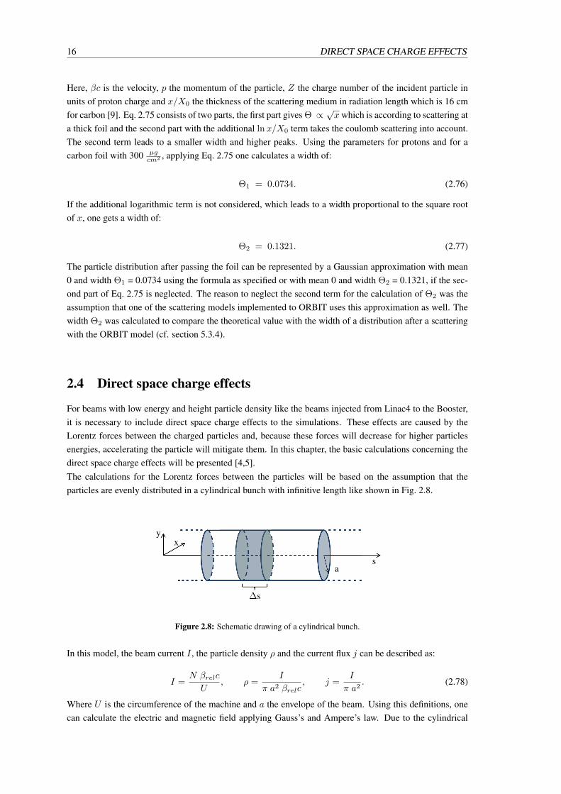
For beams with low energy and height particle density like the beams injected from Linac4 to the Booster,it is necessary to include direct space charge effects to the simulations. These effects are caused by theLorentz forces between the charged particles and, because these forces will decrease for higher particlesenergies, accelerating the particle will mitigate them. In this chapter, the basic calculations concerning thedirect space charge effects will be presented [4,5].The calculations for the Lorentz forces between the particles will be based on the assumption that theparticles are evenly distributed in a cylindrical bunch with infinitive length like shown in Fig. 2.8.
xy
sa
∆s
Figure 2.8: Schematic drawing of a cylindrical bunch.
In this model, the beam current I , the particle density ρ and the current flux j can be described as:
I =N βrelc
U, ρ =
I
π a2 βrelc, j =
I
π a2. (2.78)
Where U is the circumference of the machine and a the envelope of the beam. Using this definitions, onecan calculate the electric and magnetic field applying Gauss’s and Ampere’s law. Due to the cylindrical
17
symmetry of the bunch with an infinite length, there are just radial components for the electric and az-imuthal components for the magnetic field caused by the particle distribution.
The electric field can be calculated by:
ε0
∫∂S
~E d~S =
∫∂V
dV (2.79)
⇔ 2π r s ε0 Er = ρ π r2 s
⇔ Er =ρ r
2ε0Insert ρ from Eq.2.78
=I r
π a2 βrelc, , (2.80)
and the magnetic field can be calculated by:
∫∂r
~B d~r = µ0
∫∂S
~j d~S (2.81)
⇔ 2 s Bφ = µ0 j r s
⇔ Bφ =µ0 j r
2. (2.82)
Use Bφ = βrel
c Er to calculate the Lorentz forces on the particles which will be needed for the equation ofmotion:
~F = q( ~E − ~v × ~B) (2.83)
= q(Er − βrelγBφ)
= q(1− β2rel)Er
=qErγ2rel
. (2.84)
Insert d2rdt2 = β2
relc2 d2rds2 and Eq. 2.80 to the equation of motion which is given by Eq. 2.85:
γrelmd2r
dt2=
q Erγ2rel
(2.85)
⇔ d2r
ds2=
q I
2π mε0 a2 β3rel γ
3rel c
3r
=κ
a2r. (2.86)
The general perveance
κ =q I
2π mε0 β3rel γ
3rel c
3, (2.87)
is a notion used in the description of charged particle beams. The value of the perveance indicates how sig-nificant the space charge effect is on the beam’s motion. The term is used primarily for low-energy beams,in which motion is dominated by the space charge [10].

18 DIRECT SPACE CHARGE EFFECTS
κ can also be defined as:
using the Alven-current:
κ =2 I
I0β3relγ
3rel
, (2.88)
I0 =4π ε0 mc
3
q. (2.89)
For the further calculations, the smooth approximation model will be used with the same tune in both planesQ = Qx = Qy , also the same emittances ε = εx = εy and the same focusing strength at all positions of thelattice k0 = kx(s) = ky(s).
The focusing strength is expressed by: k0 = 2π Q0
U .
Due to the fact that the focusing strength is the same at all positions, also the beta function is constant.
β(s) = β0 =1
k0=
U
2π Q0. (2.90)
Then, the envelope equation is given by:
K a− ε2
a3= 0 with (2.91)
K = k0 a−κ
a2. (2.92)
The combined focusing strength K shows that the space charge effects affect on the beam like a defocusingquadrupole with strength κ.Using this fact, the calculations of the tune shift caused by the direct space charge effects can be achieved.
The general formula for the tune shift is:
∆Q =1
4π
∮β(s) ∆k(s) ds (2.93)
and for the smooth approximation model:
∆Q =1
4π
∮β0
κ
a2ds Insert Eq. 2.88 (2.94)
= − C4π
I q β0a2 β3
relγ3relI0
. (2.95)
Using I from Eq. 2.78 and ε∗ = ε βrelγrel, one gets the formula for the tune shift:
∆Q = − Ne
2π I0 ε∗βrelγ2. (2.96)
The tune shift caused by the direct space charge effects is proportional to the number of particles in the ringN and inverse proportional to the normalised emittance ε and to the relativistic factors βrel and γ2rel.
∆Q ∝ N
ε∗ βrelγ2. (2.97)
19
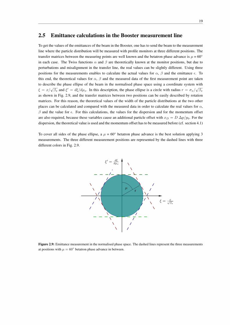
2.5 Emittance calculations in the Booster measurement line
To get the values of the emittances of the beam in the Booster, one has to send the beam to the measurementline where the particle distribution will be measured with profile monitors at three different positions. Thetransfer matrices between the measuring points are well known and the betatron phase advance is µ = 60
in each case. The Twiss functions α and β are theoretically known at the monitor positions, but due toperturbations and misalignment in the transfer line, the real values can be slightly different. Using threepositions for the measurements enables to calculate the actual values for α, β and the emittance ε. Tothis end, the theoretical values for α, β and the measured data of the first measurement point are takento describe the phase ellipse of the beam in the normalised phase space using a coordinate system withξ = x/
√βx and ξ′ = dξ/dµs. In this description, the phase ellipse is a circle with radius r = σx/
√βx
as shown in Fig. 2.9, and the transfer matrices between two positions can be easily described by rotationmatrices. For this reason, the theoretical values of the width of the particle distributions at the two otherplaces can be calculated and compared with the measured data in order to calculate the real values for α,β and the value for ε. For this calculations, the values for the dispersion and for the momentum offsetare also required, because these variables cause an additional particle offset with xD = D ∆p/p0. For thedispersion, the theoretical value is used and the momentum offset has to be measured before (cf. section 4.1)
To cover all sides of the phase ellipse, a µ = 60 betatron phase advance is the best solution applying 3measurements. The three different measurement positions are represented by the dashed lines with threedifferent colors in Fig. 2.9.
ξ′ = dξdµx
ξ = x√βx
µr
Figure 2.9: Emittance measurement in the normalised phase space. The dashed lines represent the three measurementsat positions with µ = 60 betatron phase advance in between.

20 EMITTANCE CALCULATIONS IN THE BOOSTER MEASUREMENT LINE
21
Chapter 3
The linear accelerators and the ProtonSynchrotron Booster at CERN
3.1 Proton Synchrotron Booster
In this chapter, all accelerators used for the simulations will be described. This includes Linac2 and Linac4as well as the PS Booster and, for both linacs, the injection to the Booster. Furthermore, the reason tochange from Linac2 to Linac4 and with it from a conventional multiturn injection for protons to a H− chargeexchange injection as well as the change from 50 MeV to 160 MeV injection energy will be described.
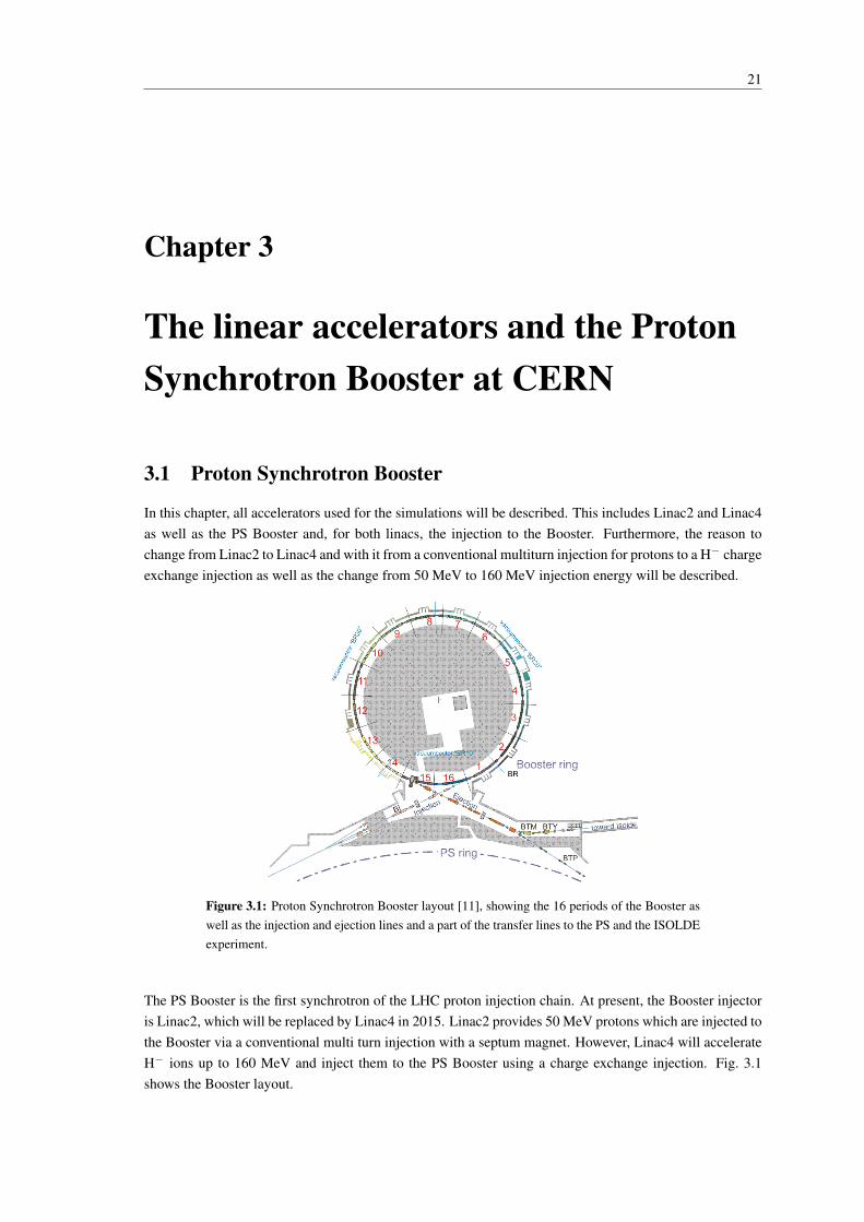
Figure 3.1: Proton Synchrotron Booster layout [11], showing the 16 periods of the Booster aswell as the injection and ejection lines and a part of the transfer lines to the PS and the ISOLDEexperiment.
The PS Booster is the first synchrotron of the LHC proton injection chain. At present, the Booster injectoris Linac2, which will be replaced by Linac4 in 2015. Linac2 provides 50 MeV protons which are injected tothe Booster via a conventional multi turn injection with a septum magnet. However, Linac4 will accelerateH− ions up to 160 MeV and inject them to the PS Booster using a charge exchange injection. Fig. 3.1shows the Booster layout.

22 PROTON SYNCHROTRON BOOSTER
L1 B1 QF QD QF B2
s
βx
βy
D
Figure 3.2: Regular period of the PS Booster.
The Booster consists of four rings, one upon the other, with a circumference of 157.08 m and a distance of36 cm between them. Each Booster ring is subdivided in 16 periods with a length of 9.82 m and all rings arefilled by one linac. As a result, fast vertical distributor and septum magnets (cf. section 3.2.1) are requiredto fill them one after the other. The motivation to stack four accelerator rings on top of each other is that thebeam intensity, provided by the Booster, can be four times higher than for one ring using the same repetitionrate. Fig. 3.2 shows a regular Booster period.
Due to the small distances between the rings, the magnets of each ring will also affect on the rings nextto them. This leads to additional multipole components, especially in ring 1 and 4, caused by the missingvertical symmetry of the magnetic fields. Thus, the performances of the Booster rings 1 and 4 is not asgood as the performance of the inner rings, in particular with the "old" working point (vertical tune one unithigher than at present) used up to 2005.
Each period contains two bending magnets as well as two horizontal focusing and one horizontal defo-cusing quadrupole magnet. The defocusing quadrupole is thereby longer than the focusing magnets. Thedrift spaces are filled with additional magnets to mitigate non-linear effects, beam diagnostic equipmentand with the acceleration cavities. The elements used for injection and ejection are in the periods 1 and 16respectively.
The injection energy with Linac2 is 50 MeV. In 1972, the Booster was built to accelerate the protons upto 800 MeV, but in the meanwhile, the Booster ejection energy has been increased and the protons get
Figure 3.3: Flatted bucket of the applied double harmonic system [7].
3.1.1 Booster improvement programme 23
accelerated up to 1.4 GeV. There are also discussions about to increase the maximum energy again up to2 GeV. Either 1.4 GeV or 2 GeV will be the maximum energy with Linac4 protons, obtained by the H−
stripping, although the injection energy is higher than with Linac2. One machine circle, lasts 1.2 secondsand of which the acceleration of the protons will take a bit less than 500 ms. The protons need roughly1 µs to 0.6 µs for one turn in the Booster, due to this, they circle the Booster 500 000 times during theacceleration. To accelerate the protons, a double harmonic system with two cavities is used. The maincavity with a harmonic number h = 1 and a second cavity, positioned in period 13, with h = 2. This leadsto flatter buckets and to mitigated direct space charge effects. After accelerating the particles in the Booster,they can be directed either to the next synchrotron of the accelerator chain, the Proton Synchrotron (PS), ordirectly to the experiment ISOLDE. Fig. 3.3 shows a bucket for a double harmonic system calculated andused for the simulations like presented in this thesis.
3.1.1 Booster improvement programme
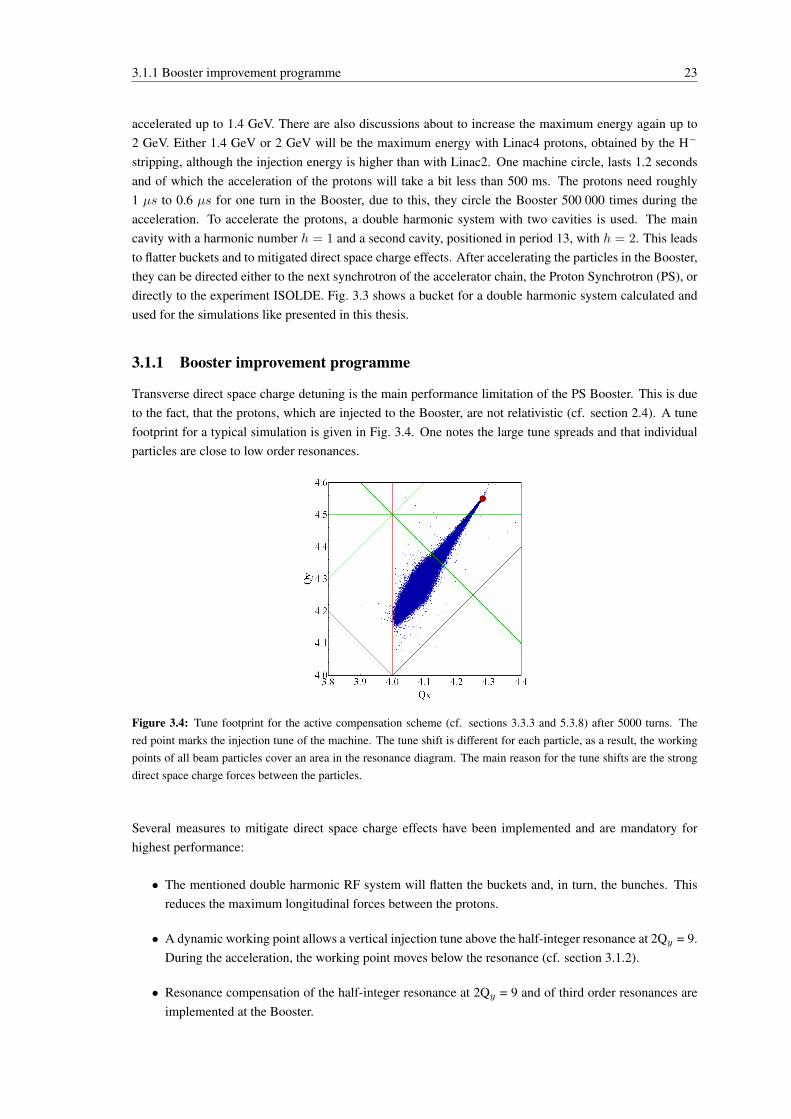
Transverse direct space charge detuning is the main performance limitation of the PS Booster. This is dueto the fact, that the protons, which are injected to the Booster, are not relativistic (cf. section 2.4). A tunefootprint for a typical simulation is given in Fig. 3.4. One notes the large tune spreads and that individualparticles are close to low order resonances.
Figure 3.4: Tune footprint for the active compensation scheme (cf. sections 3.3.3 and 5.3.8) after 5000 turns. Thered point marks the injection tune of the machine. The tune shift is different for each particle, as a result, the workingpoints of all beam particles cover an area in the resonance diagram. The main reason for the tune shifts are the strongdirect space charge forces between the particles.
Several measures to mitigate direct space charge effects have been implemented and are mandatory forhighest performance:
• The mentioned double harmonic RF system will flatten the buckets and, in turn, the bunches. Thisreduces the maximum longitudinal forces between the protons.
• A dynamic working point allows a vertical injection tune above the half-integer resonance at 2Qy = 9.During the acceleration, the working point moves below the resonance (cf. section 3.1.2).
• Resonance compensation of the half-integer resonance at 2Qy = 9 and of third order resonances areimplemented at the Booster.
24 PSB INJECTION WITH LINAC2
• The Laslett tune shift, caused by the direct space charge effects (cf. section 2.4), is depending on therelativistic factors βrel and γrel, the normalised emittance ε∗ and on the number of particles N in thering:
∆Q =N
ε∗ βrel γ2rel(3.1)
A higher beam energy leads to a smaller Laslett tune shift. If the same ∆Q can be accepted and thesame normalised emittance should be used, a higher injection energy allows higher intensity. It isessential for 50 MeV and 160 MeV protons that:
(βrel γ2rel)160MeV = 2 (βrel γ
2rel)50MeV . (3.2)
The factor 2 for the βrel γ2rel allows to double the beam intensity keeping the same emittances andLaslett tune shifts. As a result, the launch of the Linac4 will allow higher intensity beams acceleratedin the Booster.
3.1.2 Variable tune
To avoid a tune footprint crossing of the integer resonances at Qx = 4 or Qy = 4, in spite of a tune shift ofroughly ∆Q = −0.5 in vertical plane, the injection working point of the PS Booster has to be, at least forhight intensity beam, above the vertical half-integer resonance at 2Qy = 9. Due to this, the tune footprintwill cross the half-integer resonance which can lead to particle losses. But the number of lost particles willbe smaller than for a crossing of an integer resonance.
The direct space charge effects and the size of the tune footprint are related to the energy of the beam (cfEq. 3.1.1). During acceleration, the tune footprint will shrink and the machine tune can be moved below thehalf-integer resonance without pushing the particles over one of the integer resonances Qy = 4 or Qx = 4.
3.2 PSB injection with Linac2
Linac2 provides pulsed 0.83 Hz proton beams with a maximum beam current of 175 mA and an energyof 50 Mev. First beam in Linac2 was accelerated to 50 MeV on September 6th in 1978 and the operationwith Linac2 started in 1979. Linac2 is a three tank, post coupled stabilised, drift tube linac based on anAlvarez structure and with quadrupole focusing. The first pre-accelerator for Linac2 was a Cockcroft-Walton accelerator which is now replaced by a four vane radio frequency quadrupole with injection energyof 92 KeV and ejection energy of 750 KeV. The source of Linac2 is of duoplasmatron type delivering amaximum current of 300 mA [12]. The RF voltage of the Booster cavities is set to the minimum possibleduring injection (negligible for beam dynamics). After injection, the capturing of the beam takes about 1ms which is in the range of the synchrotron oscillation period and not adiabatic. The duration of the captureprocess is the compromise between two contrarily requirements:
• The magnetic field ramp rate at injection should be large to accelerate the beam and, as a result,reduce direct space charge effects quickly. This leads to short duration of the capture process.
• Capture should be slow to reduce non-adiabatic effects.
3.2.1 Injection and ejection hardware 25
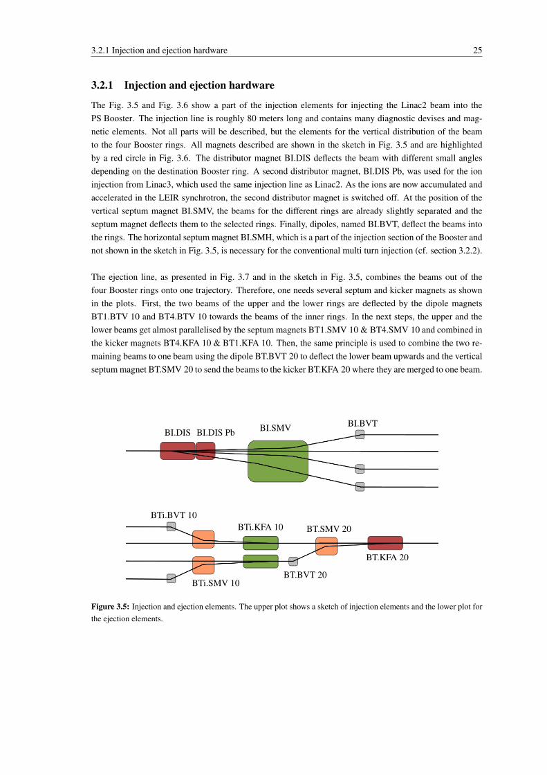
3.2.1 Injection and ejection hardware
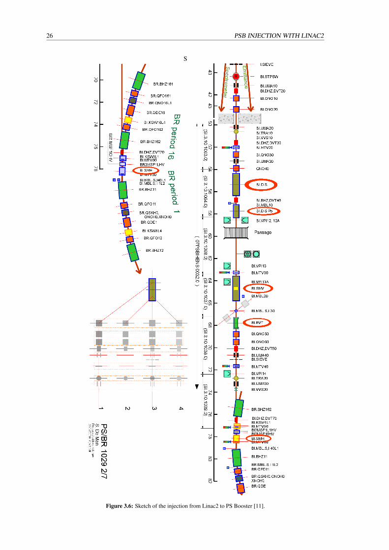
The Fig. 3.5 and Fig. 3.6 show a part of the injection elements for injecting the Linac2 beam into thePS Booster. The injection line is roughly 80 meters long and contains many diagnostic devises and mag-netic elements. Not all parts will be described, but the elements for the vertical distribution of the beamto the four Booster rings. All magnets described are shown in the sketch in Fig. 3.5 and are highlightedby a red circle in Fig. 3.6. The distributor magnet BI.DIS deflects the beam with different small anglesdepending on the destination Booster ring. A second distributor magnet, BI.DIS Pb, was used for the ioninjection from Linac3, which used the same injection line as Linac2. As the ions are now accumulated andaccelerated in the LEIR synchrotron, the second distributor magnet is switched off. At the position of thevertical septum magnet BI.SMV, the beams for the different rings are already slightly separated and theseptum magnet deflects them to the selected rings. Finally, dipoles, named BI.BVT, deflect the beams intothe rings. The horizontal septum magnet BI.SMH, which is a part of the injection section of the Booster andnot shown in the sketch in Fig. 3.5, is necessary for the conventional multi turn injection (cf. section 3.2.2).
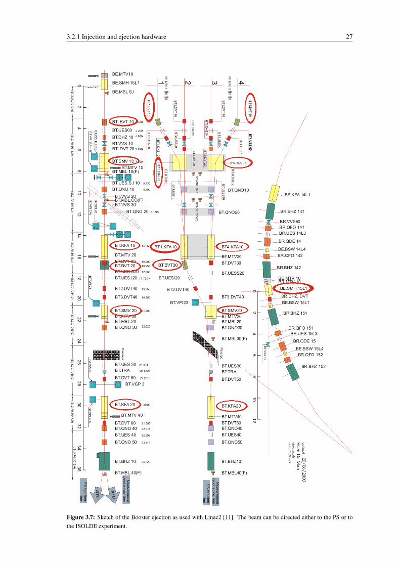
The ejection line, as presented in Fig. 3.7 and in the sketch in Fig. 3.5, combines the beams out of thefour Booster rings onto one trajectory. Therefore, one needs several septum and kicker magnets as shownin the plots. First, the two beams of the upper and the lower rings are deflected by the dipole magnetsBT1.BTV 10 and BT4.BTV 10 towards the beams of the inner rings. In the next steps, the upper and thelower beams get almost parallelised by the septum magnets BT1.SMV 10 & BT4.SMV 10 and combined inthe kicker magnets BT4.KFA 10 & BT1.KFA 10. Then, the same principle is used to combine the two re-maining beams to one beam using the dipole BT.BVT 20 to deflect the lower beam upwards and the verticalseptum magnet BT.SMV 20 to send the beams to the kicker BT.KFA 20 where they are merged to one beam.
BI.DIS BI.DIS Pb BI.SMV BI.BVT
BTi.BVT 10
BTi.SMV 10
BTi.KFA 10
BT.BVT 20
BT.SMV 20
BT.KFA 20
Figure 3.5: Injection and ejection elements. The upper plot shows a sketch of injection elements and the lower plot forthe ejection elements.
26 PSB INJECTION WITH LINAC2
S
Figure 3.6: Sketch of the injection from Linac2 to PS Booster [11].
3.2.1 Injection and ejection hardware 27
Figure 3.7: Sketch of the Booster ejection as used with Linac2 [11]. The beam can be directed either to the PS or tothe ISOLDE experiment.
28 PSB INJECTION WITH LINAC4
3.2.2 Conventional multi turn injection
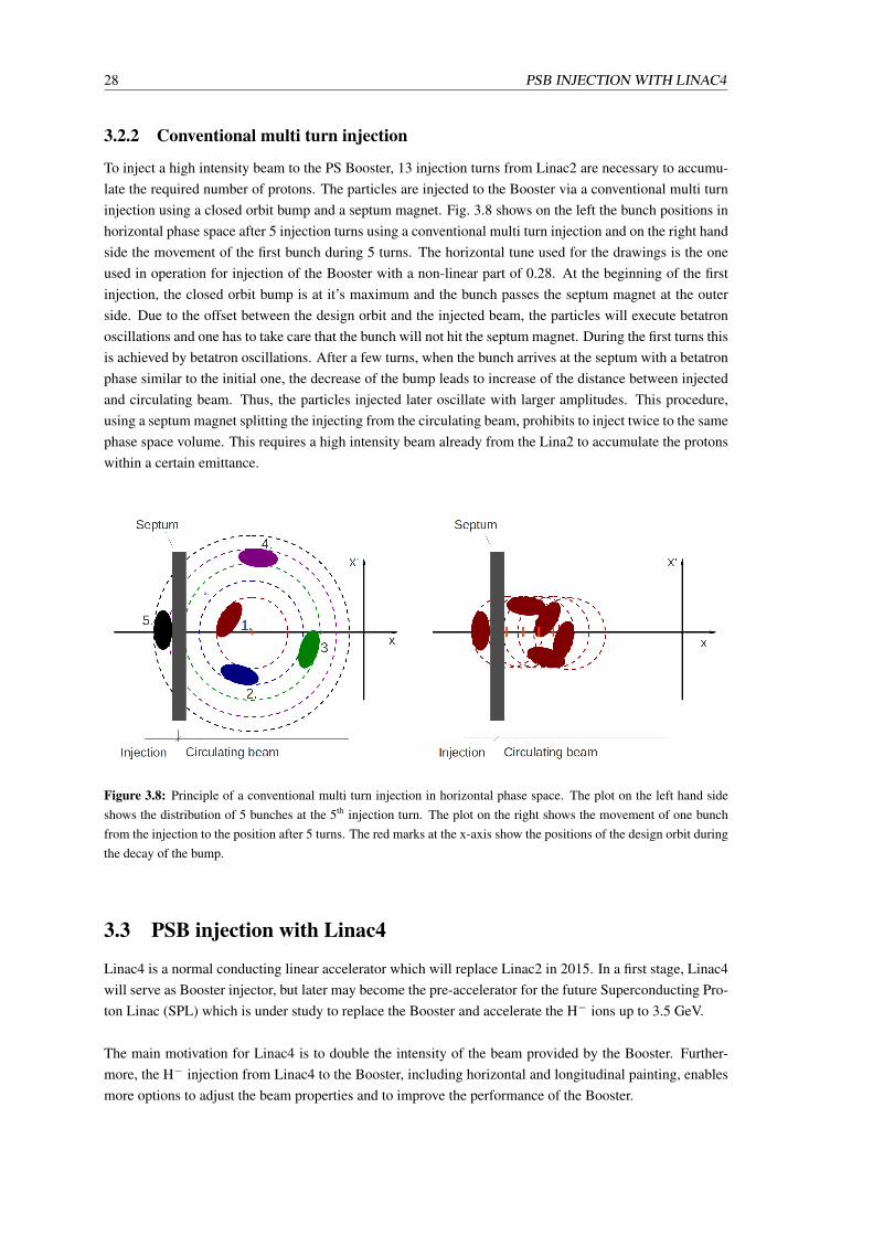
To inject a high intensity beam to the PS Booster, 13 injection turns from Linac2 are necessary to accumu-late the required number of protons. The particles are injected to the Booster via a conventional multi turninjection using a closed orbit bump and a septum magnet. Fig. 3.8 shows on the left the bunch positions inhorizontal phase space after 5 injection turns using a conventional multi turn injection and on the right handside the movement of the first bunch during 5 turns. The horizontal tune used for the drawings is the oneused in operation for injection of the Booster with a non-linear part of 0.28. At the beginning of the firstinjection, the closed orbit bump is at it’s maximum and the bunch passes the septum magnet at the outerside. Due to the offset between the design orbit and the injected beam, the particles will execute betatronoscillations and one has to take care that the bunch will not hit the septum magnet. During the first turns thisis achieved by betatron oscillations. After a few turns, when the bunch arrives at the septum with a betatronphase similar to the initial one, the decrease of the bump leads to increase of the distance between injectedand circulating beam. Thus, the particles injected later oscillate with larger amplitudes. This procedure,using a septum magnet splitting the injecting from the circulating beam, prohibits to inject twice to the samephase space volume. This requires a high intensity beam already from the Lina2 to accumulate the protonswithin a certain emittance.
Figure 3.8: Principle of a conventional multi turn injection in horizontal phase space. The plot on the left hand sideshows the distribution of 5 bunches at the 5th injection turn. The plot on the right shows the movement of one bunchfrom the injection to the position after 5 turns. The red marks at the x-axis show the positions of the design orbit duringthe decay of the bump.
3.3 PSB injection with Linac4
Linac4 is a normal conducting linear accelerator which will replace Linac2 in 2015. In a first stage, Linac4will serve as Booster injector, but later may become the pre-accelerator for the future Superconducting Pro-ton Linac (SPL) which is under study to replace the Booster and accelerate the H− ions up to 3.5 GeV.
The main motivation for Linac4 is to double the intensity of the beam provided by the Booster. Further-more, the H− injection from Linac4 to the Booster, including horizontal and longitudinal painting, enablesmore options to adjust the beam properties and to improve the performance of the Booster.
3.3.1 Injection to the 4 Booster rings 29
Figure 3.9: Structure of Linac4 [14].
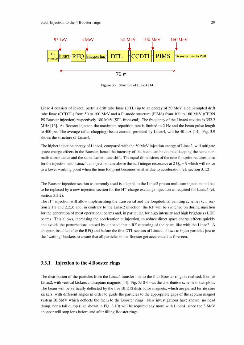
Linac 4 consists of several parts: a drift tube linac (DTL) up to an energy of 50 MeV, a cell-coupled drifttube linac (CCDTL) from 50 to 100 MeV and a Pi-mode structure (PIMS) from 100 to 160 MeV (CERNPS Booster injection) respectively 180 MeV (SPL front-end). The frequency of the Linac4 cavities is 352.2MHz [13]. As Booster injector, the maximum repetition rate is limited to 2 Hz and the beam pulse lengthto 400 µs. The average (after chopping) beam current, provided by Linac4, will be 40 mA [14]. Fig. 3.9shows the structure of Linac4.
The higher injection energy of Linac4, compared with the 50 MeV injection energy of Linac2, will mitigatespace charge effects in the Booster, hence the intensity of the beam can be doubled keeping the same nor-malised emittance and the same Laslett tune shift. The equal dimensions of the tune footprint requires, alsofor the injection with Linac4, an injection tune above the half integer resonance at 2 Qy = 9 which will moveto a lower working point when the tune footprint becomes smaller due to acceleration (cf. section 3.1.2).
The Booster injection section as currently used is adapted to the Linac2 proton multiturn injection and hasto be replaced by a new injection section for the H− charge exchange injection as required for Linac4 (cf.section 3.3.2).The H− injection will allow implementing the transversal and the longitudinal painting schemes (cf. sec-tion 2.1.8 and 2.2.3) and, in contrary to the Linac2 injection, the RF will be switched on during injectionfor the generation of most operational beams and, in particular, for high intensity and high brightness LHCbeams. This allows, increasing the acceleration at injection, to reduce direct space charge effects quicklyand avoids the perturbations caused by a nonadiabatic RF capturing of the beam like with the Linac2. Achopper, installed after the RFQ and before the first DTL section of Linac4, allows to inject particles just tothe "waiting" buckets to assure that all particles in the Booster get accelerated as foreseen.
3.3.1 Injection to the 4 Booster rings
The distribution of the particles from the Linac4 transfer line to the four Booster rings is realised, like forLinac2, with vertical kickers and septum magnets [14]. Fig. 3.10 shows the distribution scheme in two plots.The beam will be vertically deflected by the five BI.DIS distributor magnets, which are pulsed ferrite corekickers, with different angles in order to guide the particles to the appropriate gaps of the septum magnetsystem BI.SMV which deflects the them to the Booster rings. New investigations have shown, no headdump, nor a tail dump (like shown in Fig. 3.10) will be required any more with Linac4, since the 3 MeVchopper will stop ions before and after filling Booster rings.
30 PSB INJECTION WITH LINAC4
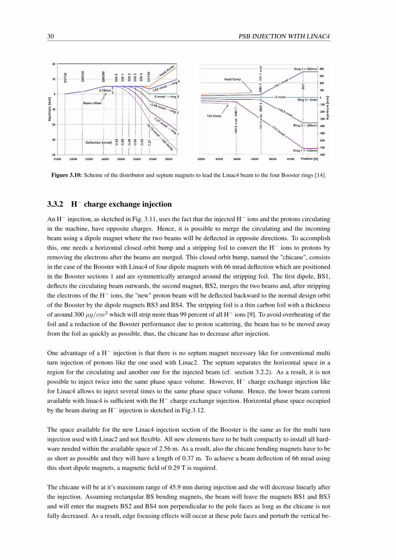
Figure 3.10: Scheme of the distributor and septum magnets to lead the Linac4 beam to the four Booster rings [14].
3.3.2 H− charge exchange injection
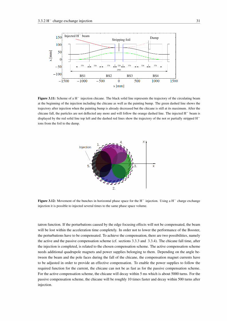
An H− injection, as sketched in Fig. 3.11, uses the fact that the injected H− ions and the protons circulatingin the machine, have opposite charges. Hence, it is possible to merge the circulating and the incomingbeam using a dipole magnet where the two beams will be deflected in opposite directions. To accomplishthis, one needs a horizontal closed orbit bump and a stripping foil to convert the H− ions to protons byremoving the electrons after the beams are merged. This closed orbit bump, named the "chicane", consistsin the case of the Booster with Linac4 of four dipole magnets with 66 mrad deflection which are positionedin the Booster sections 1 and are symmetrically arranged around the stripping foil. The first dipole, BS1,deflects the circulating beam outwards, the second magnet, BS2, merges the two beams and, after strippingthe electrons of the H− ions, the "new" proton beam will be deflected backward to the normal design orbitof the Booster by the dipole magnets BS3 and BS4. The stripping foil is a thin carbon foil with a thicknessof around 300 µg/cm2 which will strip more than 99 percent of all H− ions [9]. To avoid overheating of thefoil and a reduction of the Booster performance due to proton scattering, the beam has to be moved awayfrom the foil as quickly as possible, thus, the chicane has to decrease after injection.
One advantage of a H− injection is that there is no septum magnet necessary like for conventional multiturn injection of protons like the one used with Linac2. The septum separates the horizontal space in aregion for the circulating and another one for the injected beam (cf. section 3.2.2). As a result, it is notpossible to inject twice into the same phase space volume. However, H− charge exchange injection likefor Linac4 allows to inject several times to the same phase space volume. Hence, the lower beam currentavailable with linac4 is sufficient with the H− charge exchange injection. Horizontal phase space occupiedby the beam during an H− injection is sketched in Fig.3.12.
The space available for the new Linac4 injection section of the Booster is the same as for the multi turninjection used with Linac2 and not flexible. All new elements have to be built compactly to install all hard-ware needed within the available space of 2.56 m. As a result, also the chicane bending magnets have to beas short as possible and they will have a length of 0.37 m. To achieve a beam deflection of 66 mrad usingthis short dipole magnets, a magnetic field of 0.29 T is required.
The chicane will be at it’s maximum range of 45.9 mm during injection and she will decrease linearly afterthe injection. Assuming rectangular BS bending magnets, the beam will leave the magnets BS1 and BS3and will enter the magnets BS2 and BS4 non perpendicular to the pole faces as long as the chicane is notfully decreased. As a result, edge focusing effects will occur at these pole faces and perturb the vertical be-
3.3.2 H− charge exchange injection 31
BS1 BS2 BS3 BS4
Injected H− beamStripping foil Dump
370 370 370 370326 220 326
2560
Figure 3.11: Scheme of a H− injection chicane. The black solid line represents the trajectory of the circulating beamat the beginning of the injection including the chicane as well as the painting bump. The green dashed line shows thetrajectory after injection when the painting bump is already decreased but the chicane is still at its maximum. After thechicane fall, the particles are not deflected any more and will follow the orange dashed line. The injected H− beam isdisplayed by the red solid line top left and the dashed red lines show the trajectory of the not or partially stripped H−
ions from the foil to the dump.
Figure 3.12: Movement of the bunches in horizontal phase space for the H− injection. Using a H− charge exchangeinjection it is possible to injected several times to the same phase space volume.
tatron function. If the perturbations caused by the edge focusing effects will not be compensated, the beamwill be lost within the acceleration time completely. In order not to lower the performance of the Booster,the perturbations have to be compensated. To achieve the compensation, there are two possibilities, namelythe active and the passive compensation scheme (cf. sections 3.3.3 and 3.3.4). The chicane fall time, afterthe injection is completed, is related to the chosen compensation scheme. The active compensation schemeneeds additional quadrupole magnets and power supplies belonging to them. Depending on the angle be-tween the beam and the pole faces during the fall of the chicane, the compensation magnet currents haveto be adjusted in order to provide an effective compensation. To enable the power supplies to follow therequired function for the current, the chicane can not be as fast as for the passive compensation scheme.For the active compensation scheme, the chicane will decay within 5 ms which is about 5000 turns. For thepassive compensation scheme, the chicane will be roughly 10 times faster and decay within 500 turns afterinjection.
32 PSB INJECTION WITH LINAC4
In addition to the injection chicane, the painting bump is required to implement the horizontal painting.The painting bump is, such as the chicane, a closed orbit bump around the injection area. The height of thepainting bump at the beginning of the injection is, depending on the beam and other injection parameters,35 mm and he is realised with 4 bumper magnets in the sections 1,2 and 16. Due to the larger distance ofthe magnets from the injection point, the deflections of the magnets can be smaller than for the BS mag-nets, thus, there are no significant perturbations due to edge focusing effects caused by the painting bump.Contrary to the chicane, the painting bump starts to decay already during the injection to control the fillingof the horizontal phase ellipse. For a hight intensity beam with 1.6 × 10¹³ protons per ring, injected within100 turns and with a maximum painting bump height of 25 mm, the painting bump decreases within 280 µs.
3.3.3 Active compensation
The active compensation is realised with additional quadrupole components at existing quadrupole magnetsin the Booster lattice. Focusing errors, like the edge focusing effects at the BS magnets of the chicane, canbe compensated efficiently at ± 90 (n ∈ N) betatron phase advance from the perturbation. It is necessaryto choose quadrupole magnets which fulfill these requirements for the vertical phase space, where latticeperturbations are strong, since the tune is close to a half-integer resonance. Appropriate locations for ad-ditional quadrupole components are the defocusing quadrupole magnets in the sections 3 and 14. Tab. 3.1shows the beta function and the betatron phase advances at the chosen positions.
Table 3.1: Beta functions and betatron phase advance at the position of the active compensation. µx and µy show thebetatron phase advance between the edge focusing at the BS magnets and the magnets where the compensation takesplace.
Period βx [m] βy [m] µx [2π] µy [2π]3 3.709 16.574 0.668 0.72014 3.708 16.584 -0.668 -0.720
The beta function in the periods 3 and 14 are slightly different, in spite of the same positions in the respectiveperiods, this is due to the fact that the painting bump is not completely symmetric around the injection point.As the compensation will be placed on defocusing magnets, the vertical beta functions are larger than thehorizontal ones. This leads to effective compensation of the perturbations in vertical plane and to smallperturbations in horizontal plane. The betatron phase advances at the compensation positions are:
0.720 2π = 1.44 π ≈ 1.5 π (3.3)
0.668 2π = 1.34 π ≈ 1.5 π, (3.4)
so that, the betatron phase advances at the compensation positions are almost at the required values of± n × 90 with n ∈ N.
3.3.4 Passive compensation
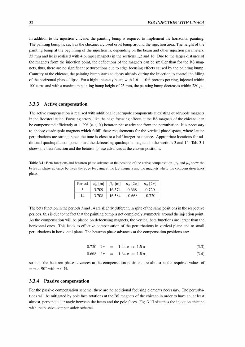
For the passive compensation scheme, there are no additional focusing elements necessary. The perturba-tions will be mitigated by pole face rotations at the BS magnets of the chicane in order to have an, at leastalmost, perpendicular angle between the beam and the pole faces. Fig. 3.13 sketches the injection chicanewith the passive compensation scheme.
33
BS1 BS2 BS3 BS4
Figure 3.13: Passive compensation scheme with pole face rotations. The rotated pole faces avoid almost the edgefocusing due to the fact, that the beam is nearly perpendicular to the magnets pole faces.
Due to the tight space available, there is not enough space left to realise the pole face rotations. Hence, thedecision was made to implement the passive compensation by adding gradients to the magnetic field of theBS magnet, which is equivalent to pole face rotations.
Due to the fact that the chicane decreases after injection and the pole face rotations are fixed, it is notpossible to mitigate the perturbations during injection and during the chicane fall. As a result, one has tofind a compensation setting which gives the best results (cf. section 5.3.7 and 5.3.8).
3.4 PS Booster measurement line
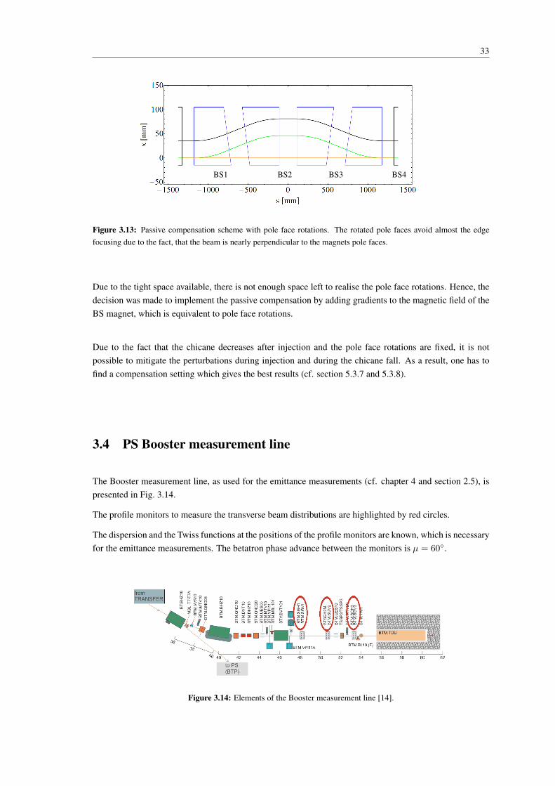
The Booster measurement line, as used for the emittance measurements (cf. chapter 4 and section 2.5), ispresented in Fig. 3.14.
The profile monitors to measure the transverse beam distributions are highlighted by red circles.
The dispersion and the Twiss functions at the positions of the profile monitors are known, which is necessaryfor the emittance measurements. The betatron phase advance between the monitors is µ = 60.
Figure 3.14: Elements of the Booster measurement line [14].

34 PS BOOSTER MEASUREMENT LINE

Chapter 4
Measurements
4.1 Beam properties
To run simulations of the injection and acceleration of a beam in the Booster for the results which are pre-sented in this thesis, it was necessary to know the desired beam properties and, in particular, the emittancesto adapt the simulation settings to this values. As the PS Booster has been running for many years usingLinac2 as injector and as the beam parameters are the same for Linac2 and linac4 injection, it is possible tomeasure the standard emittances of different operational beams and apply them to simulations for Linac4.These measurements were carried out for a high intensity beam required for the CNGS (CERN Neutrinos toGran Sasso) experiment and for the LHC25A (LHC nominal) beam. The emittances for the high intensitybeam are required for the simulations presented in this thesis and the LHC nominal beam emittances forsimulations which will be carried out in further studies.
To study the emittances, the beam investigated has to be sent to the measurement line of the Booster. Note,that just one out of the four Booster rings was used for the measurements to avoid effects by overlappingbeams of the different rings. To have, at least, two sets of data, the measurements were carried out withbeams from the Booster rings 3 and 4.
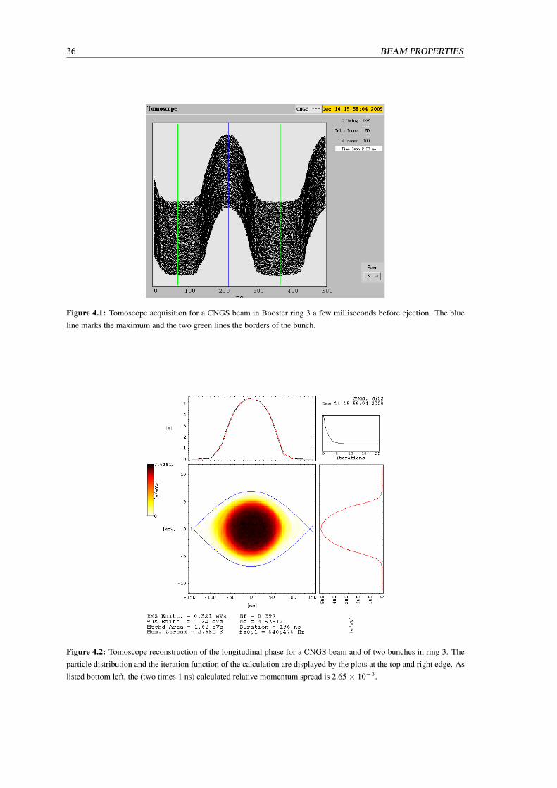
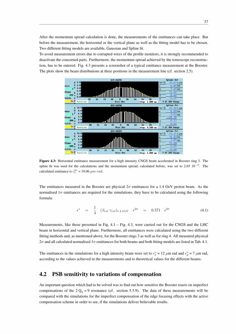
Before the emittance measurement can be started, the relative momentum spread of the beam, necessary forthe calculation of the particles offset due to dispersion (cf. section 2.5), has to be evaluated. To this end, atool called the Tomoscope has to be used to define the bucket. Fig. 4.1 shows several bunch shape measure-ments done at regular intervals (every 50th revolution) during about one and a half synchrotron oscillationperiods. These data serve to reconstruct the longitudinal phase space distribution depicted in Fig. 4.2 bytomographic reconstruction.
36 BEAM PROPERTIES
Figure 4.1: Tomoscope acquisition for a CNGS beam in Booster ring 3 a few milliseconds before ejection. The blueline marks the maximum and the two green lines the borders of the bunch.
Figure 4.2: Tomoscope reconstruction of the longitudinal phase for a CNGS beam and of two bunches in ring 3. Theparticle distribution and the iteration function of the calculation are displayed by the plots at the top and right edge. Aslisted bottom left, the (two times 1 ns) calculated relative momentum spread is 2.65 × 10⁻³.
37
After the momentum spread calculation is done, the measurements of the emittances can take place. Butbefore the measurement, the horizontal or the vertical plane as well as the fitting model has to be chosen.Two different fitting models are available, Gaussian and Spline fit.To avoid measurement errors due to corrupted wires of the profile monitors, it is strongly recommended todeactivate the concerned parts. Furthermore, the momentum spread achieved by the tomoscope reconstruc-tion, has to be entered. Fig. 4.3 presents a screenshot of a typical emittance measurement at the Booster.The plots show the beam distributions at three positions in the measurement line (cf. section 2.5).
Figure 4.3: Horizontal emittance measurement for a high intensity CNGS beam accelerated in Booster ring 3. Thespline fit was used for the calculations and the momentum spread, calculated before, was set to 2.65 10−3. Thecalculated emittance is ε2σx = 19.06 µm rad.
The emittances measured in the Booster are physical 2σ emittances for a 1.4 GeV proton beam. As thenormalised 1σ emittances are required for the simulations, they have to be calculated using the followingformula:
ε∗ =1
4(βrel γrel)1.4 GeV ε2σ = 0.571 ε2σ (4.1)
Measurements, like those presented in Fig. 4.1 – Fig. 4.3, were carried out for the CNGS and the LHCbeam in horizontal and vertical plane. Furthermore, all emittances were calculated using the two differentfitting methods and, as mentioned above, for the Booster rings 3 as well as for ring 4. All measured physical2σ and all calculated normalised 1σ emittances for both beams and both fitting models are listed in Tab. 4.1.
The emittances in the simulations for a high intensity beam were set to ε∗x = 12 µm rad and ε∗y = 7 µm rad,according to the values achieved in the measurements and to theoretical values for the different beams.
4.2 PSB sensitivity to variations of compensation
An important question which had to be solved was to find out how sensitive the Booster reacts on imperfectcompensations of the 2 Qy = 9 resonance (cf. section 5.3.9). The data of these measurements will becompared with the simulations for the imperfect compensation of the edge focusing effects with the activecompensation scheme in order to see, if the simulations deliver believable results.
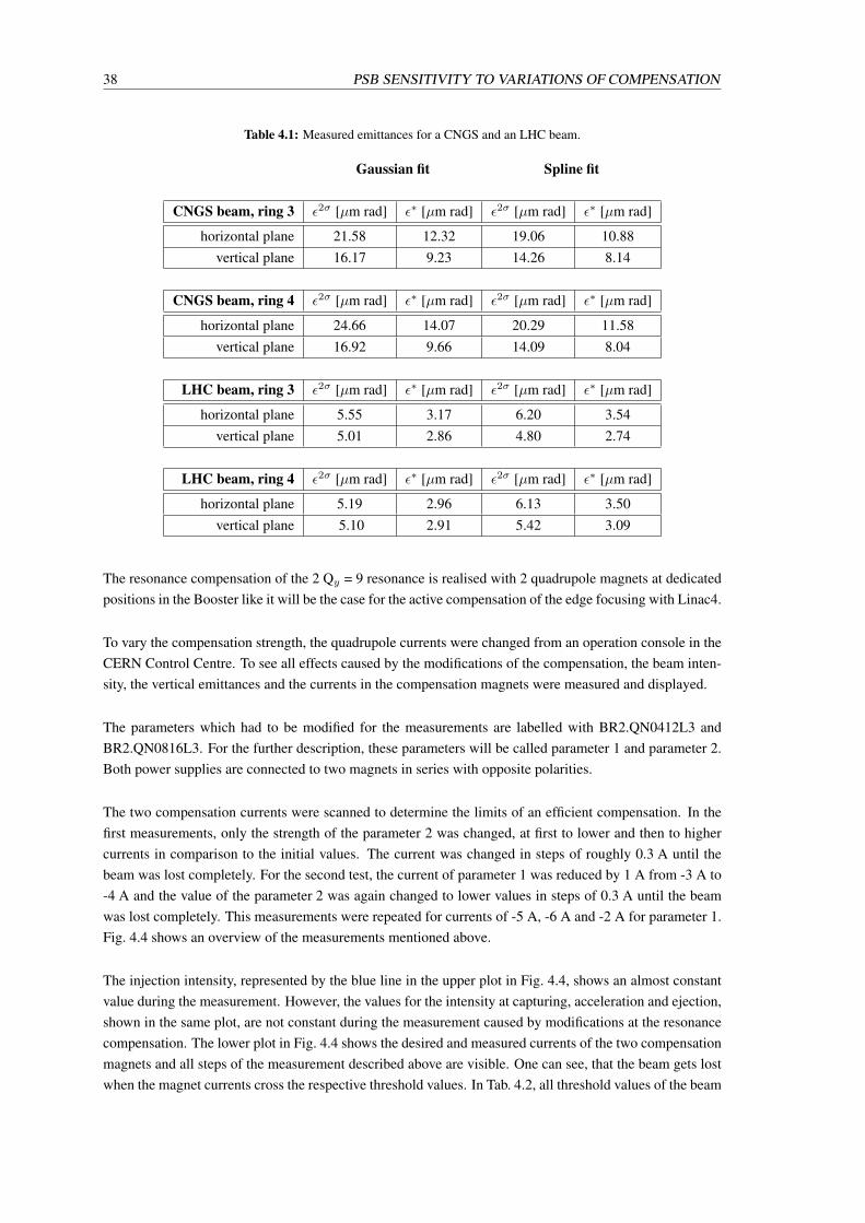
38 PSB SENSITIVITY TO VARIATIONS OF COMPENSATION
Table 4.1: Measured emittances for a CNGS and an LHC beam.
Gaussian fit Spline fit
CNGS beam, ring 3 ε2σ [µm rad] ε∗ [µm rad] ε2σ [µm rad] ε∗ [µm rad]
horizontal plane 21.58 12.32 19.06 10.88vertical plane 16.17 9.23 14.26 8.14
CNGS beam, ring 4 ε2σ [µm rad] ε∗ [µm rad] ε2σ [µm rad] ε∗ [µm rad]
horizontal plane 24.66 14.07 20.29 11.58vertical plane 16.92 9.66 14.09 8.04
LHC beam, ring 3 ε2σ [µm rad] ε∗ [µm rad] ε2σ [µm rad] ε∗ [µm rad]
horizontal plane 5.55 3.17 6.20 3.54vertical plane 5.01 2.86 4.80 2.74
LHC beam, ring 4 ε2σ [µm rad] ε∗ [µm rad] ε2σ [µm rad] ε∗ [µm rad]
horizontal plane 5.19 2.96 6.13 3.50vertical plane 5.10 2.91 5.42 3.09
The resonance compensation of the 2 Qy = 9 resonance is realised with 2 quadrupole magnets at dedicatedpositions in the Booster like it will be the case for the active compensation of the edge focusing with Linac4.
To vary the compensation strength, the quadrupole currents were changed from an operation console in theCERN Control Centre. To see all effects caused by the modifications of the compensation, the beam inten-sity, the vertical emittances and the currents in the compensation magnets were measured and displayed.
The parameters which had to be modified for the measurements are labelled with BR2.QN0412L3 andBR2.QN0816L3. For the further description, these parameters will be called parameter 1 and parameter 2.Both power supplies are connected to two magnets in series with opposite polarities.
The two compensation currents were scanned to determine the limits of an efficient compensation. In thefirst measurements, only the strength of the parameter 2 was changed, at first to lower and then to highercurrents in comparison to the initial values. The current was changed in steps of roughly 0.3 A until thebeam was lost completely. For the second test, the current of parameter 1 was reduced by 1 A from -3 A to-4 A and the value of the parameter 2 was again changed to lower values in steps of 0.3 A until the beamwas lost completely. This measurements were repeated for currents of -5 A, -6 A and -2 A for parameter 1.Fig. 4.4 shows an overview of the measurements mentioned above.
The injection intensity, represented by the blue line in the upper plot in Fig. 4.4, shows an almost constantvalue during the measurement. However, the values for the intensity at capturing, acceleration and ejection,shown in the same plot, are not constant during the measurement caused by modifications at the resonancecompensation. The lower plot in Fig. 4.4 shows the desired and measured currents of the two compensationmagnets and all steps of the measurement described above are visible. One can see, that the beam gets lostwhen the magnet currents cross the respective threshold values. In Tab. 4.2, all threshold values of the beam
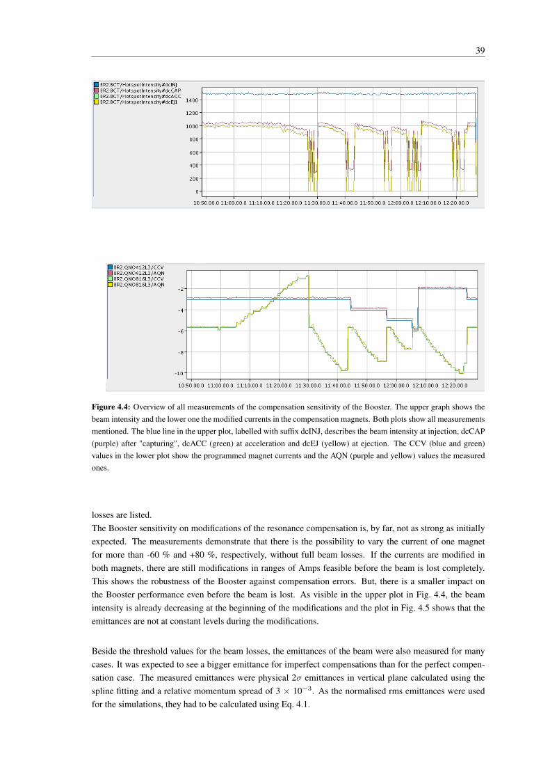
39
Figure 4.4: Overview of all measurements of the compensation sensitivity of the Booster. The upper graph shows thebeam intensity and the lower one the modified currents in the compensation magnets. Both plots show all measurementsmentioned. The blue line in the upper plot, labelled with suffix dcINJ, describes the beam intensity at injection, dcCAP(purple) after "capturing", dcACC (green) at acceleration and dcEJ (yellow) at ejection. The CCV (blue and green)values in the lower plot show the programmed magnet currents and the AQN (purple and yellow) values the measuredones.
losses are listed.The Booster sensitivity on modifications of the resonance compensation is, by far, not as strong as initiallyexpected. The measurements demonstrate that there is the possibility to vary the current of one magnetfor more than -60 % and +80 %, respectively, without full beam losses. If the currents are modified inboth magnets, there are still modifications in ranges of Amps feasible before the beam is lost completely.This shows the robustness of the Booster against compensation errors. But, there is a smaller impact onthe Booster performance even before the beam is lost. As visible in the upper plot in Fig. 4.4, the beamintensity is already decreasing at the beginning of the modifications and the plot in Fig. 4.5 shows that theemittances are not at constant levels during the modifications.
Beside the threshold values for the beam losses, the emittances of the beam were also measured for manycases. It was expected to see a bigger emittance for imperfect compensations than for the perfect compen-sation case. The measured emittances were physical 2σ emittances in vertical plane calculated using thespline fitting and a relative momentum spread of 3 × 10⁻³. As the normalised rms emittances were usedfor the simulations, they had to be calculated using Eq. 4.1.
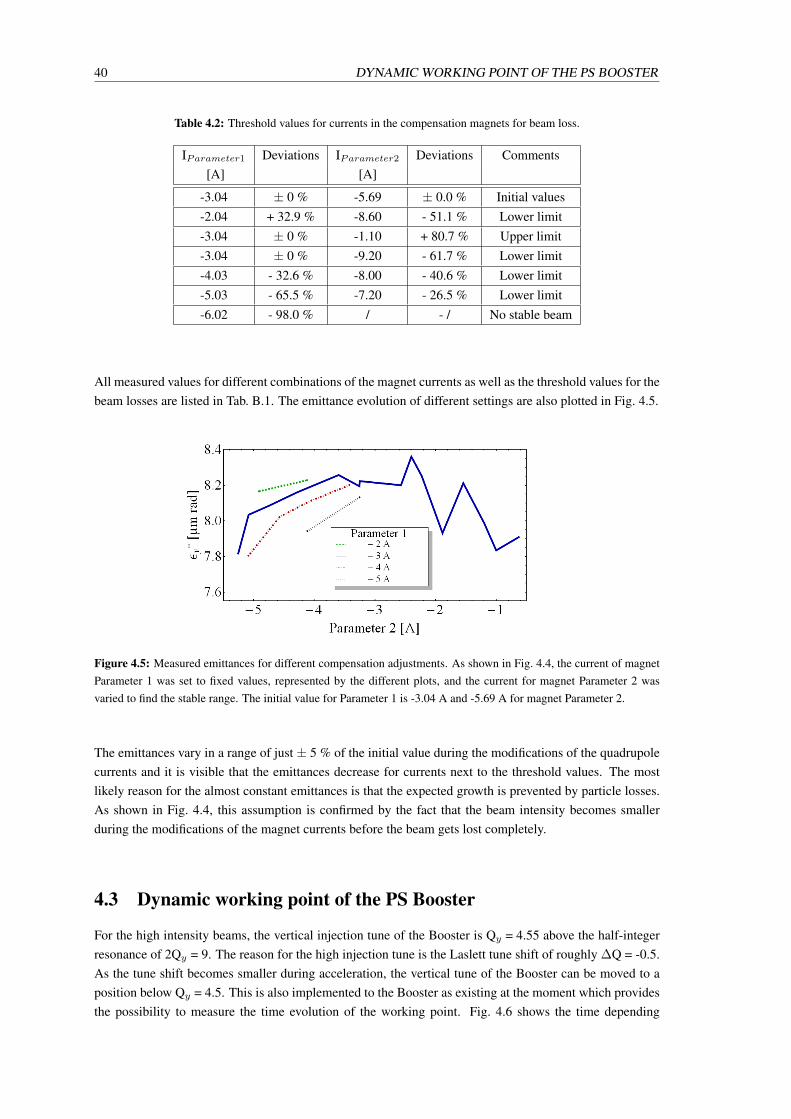
40 DYNAMIC WORKING POINT OF THE PS BOOSTER
Table 4.2: Threshold values for currents in the compensation magnets for beam loss.
IParameter1 Deviations IParameter2 Deviations Comments[A] [A]
-3.04 ± 0 % -5.69 ± 0.0 % Initial values-2.04 + 32.9 % -8.60 - 51.1 % Lower limit-3.04 ± 0 % -1.10 + 80.7 % Upper limit-3.04 ± 0 % -9.20 - 61.7 % Lower limit-4.03 - 32.6 % -8.00 - 40.6 % Lower limit-5.03 - 65.5 % -7.20 - 26.5 % Lower limit-6.02 - 98.0 % / - / No stable beam
All measured values for different combinations of the magnet currents as well as the threshold values for thebeam losses are listed in Tab. B.1. The emittance evolution of different settings are also plotted in Fig. 4.5.
Figure 4.5: Measured emittances for different compensation adjustments. As shown in Fig. 4.4, the current of magnetParameter 1 was set to fixed values, represented by the different plots, and the current for magnet Parameter 2 wasvaried to find the stable range. The initial value for Parameter 1 is -3.04 A and -5.69 A for magnet Parameter 2.
The emittances vary in a range of just ± 5 % of the initial value during the modifications of the quadrupolecurrents and it is visible that the emittances decrease for currents next to the threshold values. The mostlikely reason for the almost constant emittances is that the expected growth is prevented by particle losses.As shown in Fig. 4.4, this assumption is confirmed by the fact that the beam intensity becomes smallerduring the modifications of the magnet currents before the beam gets lost completely.
4.3 Dynamic working point of the PS Booster
For the high intensity beams, the vertical injection tune of the Booster is Qy = 4.55 above the half-integerresonance of 2Qy = 9. The reason for the high injection tune is the Laslett tune shift of roughly ∆Q = -0.5.As the tune shift becomes smaller during acceleration, the vertical tune of the Booster can be moved to aposition below Qy = 4.5. This is also implemented to the Booster as existing at the moment which providesthe possibility to measure the time evolution of the working point. Fig. 4.6 shows the time depending
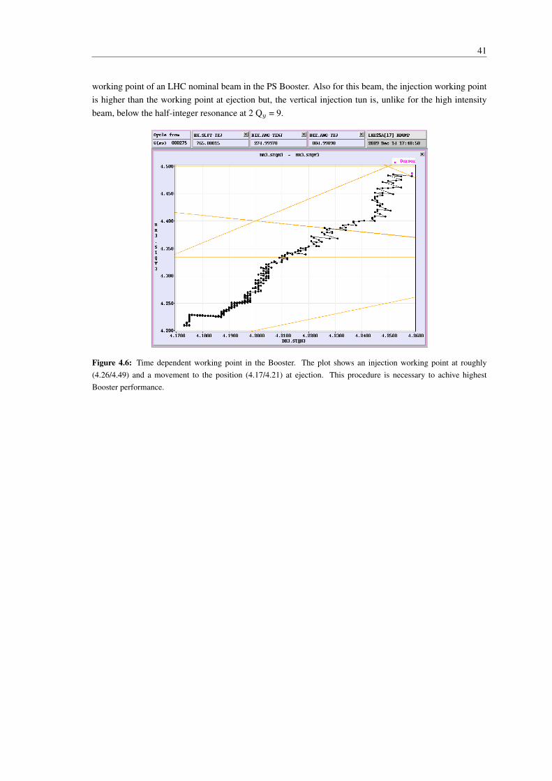
41
working point of an LHC nominal beam in the PS Booster. Also for this beam, the injection working pointis higher than the working point at ejection but, the vertical injection tun is, unlike for the high intensitybeam, below the half-integer resonance at 2 Qy = 9.
Figure 4.6: Time dependent working point in the Booster. The plot shows an injection working point at roughly(4.26/4.49) and a movement to the position (4.17/4.21) at ejection. This procedure is necessary to achive highestBooster performance.

42 DYNAMIC WORKING POINT OF THE PS BOOSTER
Chapter 5
ORBIT Simulations
5.1 About ORBIT simulations
All simulations presented in this thesis were executed using the particle tracking code ORBIT [2] (ObjectiveRing Beam Injection and Tracking). Written for studying the Spallation Neutron Source SNS which is anaccelerator- based neutron source in Oak Ridge, Tennessee, USA [15]. ORBIT was programmed to simu-late H− charge exchange injection via stripping foil from a linac to a storage ring and to simulate dynamicsof beams with strong direct space charge forces. ORBIT is capable to use multiple processing to speed upthe simulations and it is also possible to calculate the direct space charge effects between the protons.
For ORBIT runs with ”non-linear tracking”, a non documented feature, the lattice of the accelerator has tobe described in teapot [16] format. Those are generated by first using MAD8 allowing matching to tunelattice parameters and, then, processing MAD8 generated output files with the help of python [17] scriptsto generate the teapot style input files for ORBIT.
To launch an ORBIT simulation, a main file has to be called up inside the shell together with the informationhow many cores should be used. In the main file, all information about the simulation are given or they areimplemented via other files called up by the main file. One of those files is the lattice file which containsall information about elements in the ring.
Two different bumps are needed for the injection from Linac4 to the Booster (cf. section 3.3.2). The paintingbump is implemented to the simulation using the bump routing of ORBIT and the simulated magnets aredefined as thin lenses. Unfortunately, this is not possible for the chicane, because it is necessary to simulatethe edge focusing at the pole faces of the chicane magnets. It is therefore important to use bending magnetsto simulate the chicane. The injection chicane and, as a result, focusing properties introduced as well as, incase of ”active compensation”, additional compensation quadrupole components, vary with time. Such timevariations of the lattice properties were not foreseen by the ORBIT authors, but a procedure for simulationswith magnet properties varying with time has been identified [18] and applied.For this procedure, several scripts and programmes have to be used in the following order:
• Injection
– Before the injection, the particle distribution has to be generated with a Mathematica [19] filewhich creates a list of particle coordinates in 6-dim phase space including the longitudinalpainting. There is also the possibility to match the injected beam to desired Twiss parametersand the dispersion. The coordinates for each injection turn are saved to a separate file.
44 ABOUT ORBIT SIMULATIONS
– The main file which controls all further operational sequences defines all given parameters andloads a lattice file, using the initial parameters, where all lattice elements are defined. The mainfile implements also the files necessary for the acceleration of the particles.
– The next step is the start of the injection by calling each single file with the initial particledistributions in the desired order, tracking the particles between two injections for one turn anddumping the coordinates of all particles in the ring after each turn.
– The painting bump is implemented to the code as a time depending closed orbit bump whichstarts to decrease already during the injection takes place.
• Chicane fall
– After the injection is finished, the chicane will start to decrease in order to move the beam offthe foil as early as possible. To this end, all lattice elements will be deleted at each turn andreinstalled with modified values for the required magnets. All variations concerning the chicaneare depending on the deflection in the chicane magnets and this value is defined in the main fileas a variable depending on the number of turns accomplished. After the lattice is reinstalled,the acceleration files have to be installed again as well.
– The particle coordinates, the coordinates of aperture hits and the information about the particlesenergy can be dumped to files at chosen numbers of turns and all files can be saved in specifiedfolders.
• After chicane fall
– When the chicane is completely decreased, it is not necessary anymore to reload the latticeincluding all elements at each turn. Due to this, the lattice will be installed one more time withvalues adjusted to a zero deflection in the chicane magnets and again the acceleration has to beinstalled separately.
– The particle distribution as well as the other simulation parameters can still be dumped as before.
• End of simulation
– The simulation can be ended using a quit command in the main file. Before quitting, all beamparameters can be dumped again.
– To calculate the Twiss parameters, the emittances and the dispersion, which are used for allplots and further calculations in this thesis, out of the particle distribution, a Python [17] scriptis used.
– Mathematica files are used for the evaluation of the data and to produce all plots.
Limited by computer power, it is not possible to track, for example, a high intensity beam with 1.6× 10¹³
protons around the machine. To avoid this problems, a smaller number of macro particles representingthe protons are injected and tracked around the machine. A reasonable number of macro particles with anappropriate simulation duration is 500 000 (cf. section 5.3.3). Attention has been paid to make sure thatemittance blow-up and particle losses are not dominated by numerical artefacts due to a too small numberof macro particles.
The typical number of cores used for simulations with half a million macro particles and all elements in-cluded is 24. A benchmarking comparing runs using different numbers of cores led to the conclusion thatthere is no big benefit with more cores due to the fact that then the communication between the cores will
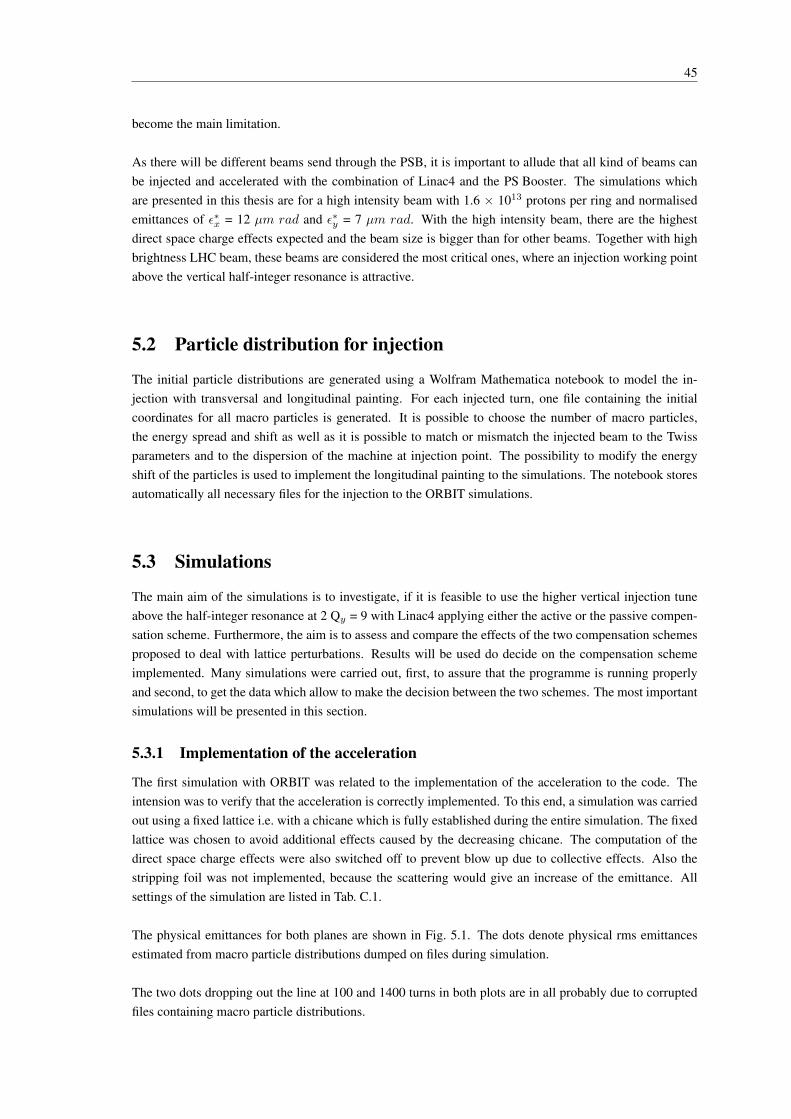
45
become the main limitation.
As there will be different beams send through the PSB, it is important to allude that all kind of beams canbe injected and accelerated with the combination of Linac4 and the PS Booster. The simulations whichare presented in this thesis are for a high intensity beam with 1.6 × 10¹³ protons per ring and normalisedemittances of ε∗x = 12 µm rad and ε∗y = 7 µm rad. With the high intensity beam, there are the highestdirect space charge effects expected and the beam size is bigger than for other beams. Together with highbrightness LHC beam, these beams are considered the most critical ones, where an injection working pointabove the vertical half-integer resonance is attractive.
5.2 Particle distribution for injection
The initial particle distributions are generated using a Wolfram Mathematica notebook to model the in-jection with transversal and longitudinal painting. For each injected turn, one file containing the initialcoordinates for all macro particles is generated. It is possible to choose the number of macro particles,the energy spread and shift as well as it is possible to match or mismatch the injected beam to the Twissparameters and to the dispersion of the machine at injection point. The possibility to modify the energyshift of the particles is used to implement the longitudinal painting to the simulations. The notebook storesautomatically all necessary files for the injection to the ORBIT simulations.
5.3 Simulations
The main aim of the simulations is to investigate, if it is feasible to use the higher vertical injection tuneabove the half-integer resonance at 2 Qy = 9 with Linac4 applying either the active or the passive compen-sation scheme. Furthermore, the aim is to assess and compare the effects of the two compensation schemesproposed to deal with lattice perturbations. Results will be used do decide on the compensation schemeimplemented. Many simulations were carried out, first, to assure that the programme is running properlyand second, to get the data which allow to make the decision between the two schemes. The most importantsimulations will be presented in this section.
5.3.1 Implementation of the acceleration
The first simulation with ORBIT was related to the implementation of the acceleration to the code. Theintension was to verify that the acceleration is correctly implemented. To this end, a simulation was carriedout using a fixed lattice i.e. with a chicane which is fully established during the entire simulation. The fixedlattice was chosen to avoid additional effects caused by the decreasing chicane. The computation of thedirect space charge effects were also switched off to prevent blow up due to collective effects. Also thestripping foil was not implemented, because the scattering would give an increase of the emittance. Allsettings of the simulation are listed in Tab. C.1.
The physical emittances for both planes are shown in Fig. 5.1. The dots denote physical rms emittancesestimated from macro particle distributions dumped on files during simulation.
The two dots dropping out the line at 100 and 1400 turns in both plots are in all probably due to corruptedfiles containing macro particle distributions.
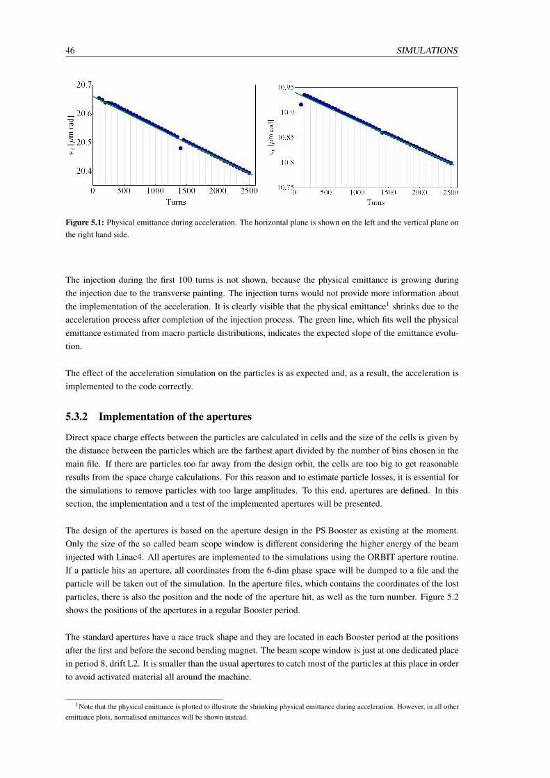
46 SIMULATIONS
Figure 5.1: Physical emittance during acceleration. The horizontal plane is shown on the left and the vertical plane onthe right hand side.
The injection during the first 100 turns is not shown, because the physical emittance is growing duringthe injection due to the transverse painting. The injection turns would not provide more information aboutthe implementation of the acceleration. It is clearly visible that the physical emittance1 shrinks due to theacceleration process after completion of the injection process. The green line, which fits well the physicalemittance estimated from macro particle distributions, indicates the expected slope of the emittance evolu-tion.
The effect of the acceleration simulation on the particles is as expected and, as a result, the acceleration isimplemented to the code correctly.
5.3.2 Implementation of the apertures
Direct space charge effects between the particles are calculated in cells and the size of the cells is given bythe distance between the particles which are the farthest apart divided by the number of bins chosen in themain file. If there are particles too far away from the design orbit, the cells are too big to get reasonableresults from the space charge calculations. For this reason and to estimate particle losses, it is essential forthe simulations to remove particles with too large amplitudes. To this end, apertures are defined. In thissection, the implementation and a test of the implemented apertures will be presented.
The design of the apertures is based on the aperture design in the PS Booster as existing at the moment.Only the size of the so called beam scope window is different considering the higher energy of the beaminjected with Linac4. All apertures are implemented to the simulations using the ORBIT aperture routine.If a particle hits an aperture, all coordinates from the 6-dim phase space will be dumped to a file and theparticle will be taken out of the simulation. In the aperture files, which contains the coordinates of the lostparticles, there is also the position and the node of the aperture hit, as well as the turn number. Figure 5.2shows the positions of the apertures in a regular Booster period.
The standard apertures have a race track shape and they are located in each Booster period at the positionsafter the first and before the second bending magnet. The beam scope window is just at one dedicated placein period 8, drift L2. It is smaller than the usual apertures to catch most of the particles at this place in orderto avoid activated material all around the machine.
1Note that the physical emittance is plotted to illustrate the shrinking physical emittance during acceleration. However, in all otheremittance plots, normalised emittances will be shown instead.
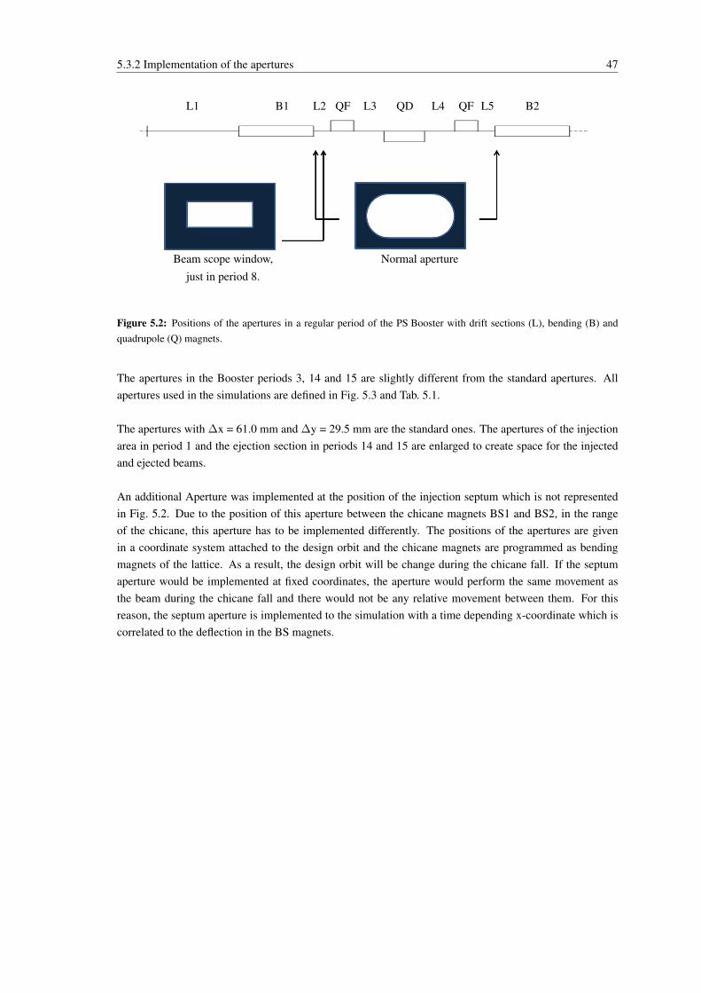
5.3.2 Implementation of the apertures 47
Beam scope window,just in period 8.
Normal aperture
L1 B1 L2 QF L3 QD L4 QF L5 B2
Figure 5.2: Positions of the apertures in a regular period of the PS Booster with drift sections (L), bending (B) andquadrupole (Q) magnets.
The apertures in the Booster periods 3, 14 and 15 are slightly different from the standard apertures. Allapertures used in the simulations are defined in Fig. 5.3 and Tab. 5.1.
The apertures with ∆x = 61.0 mm and ∆y = 29.5 mm are the standard ones. The apertures of the injectionarea in period 1 and the ejection section in periods 14 and 15 are enlarged to create space for the injectedand ejected beams.
An additional Aperture was implemented at the position of the injection septum which is not representedin Fig. 5.2. Due to the position of this aperture between the chicane magnets BS1 and BS2, in the rangeof the chicane, this aperture has to be implemented differently. The positions of the apertures are givenin a coordinate system attached to the design orbit and the chicane magnets are programmed as bendingmagnets of the lattice. As a result, the design orbit will be change during the chicane fall. If the septumaperture would be implemented at fixed coordinates, the aperture would perform the same movement asthe beam during the chicane fall and there would not be any relative movement between them. For thisreason, the septum aperture is implemented to the simulation with a time depending x-coordinate which iscorrelated to the deflection in the BS magnets.
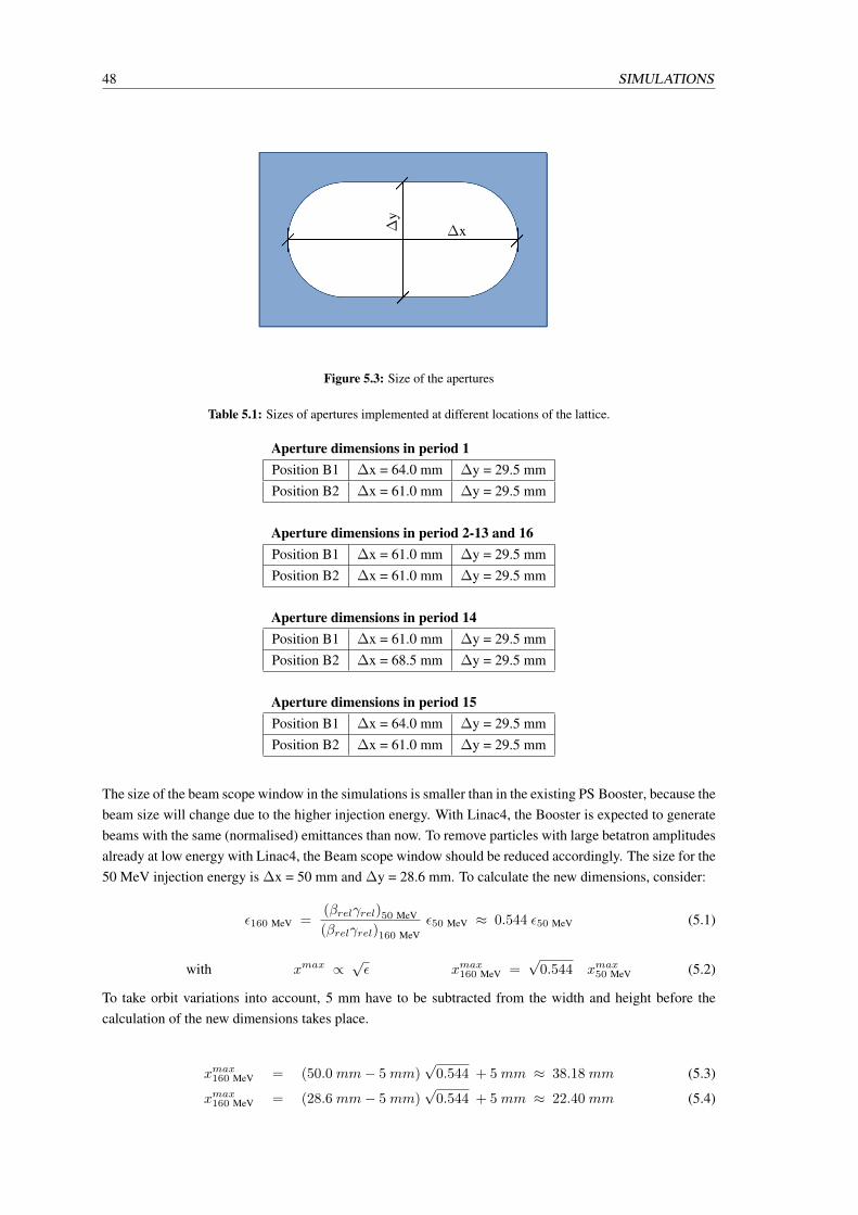
48 SIMULATIONS
∆x∆y
Figure 5.3: Size of the apertures
Table 5.1: Sizes of apertures implemented at different locations of the lattice.
Aperture dimensions in period 1Position B1 ∆x = 64.0 mm ∆y = 29.5 mmPosition B2 ∆x = 61.0 mm ∆y = 29.5 mm
Aperture dimensions in period 2-13 and 16Position B1 ∆x = 61.0 mm ∆y = 29.5 mmPosition B2 ∆x = 61.0 mm ∆y = 29.5 mm
Aperture dimensions in period 14Position B1 ∆x = 61.0 mm ∆y = 29.5 mmPosition B2 ∆x = 68.5 mm ∆y = 29.5 mm
Aperture dimensions in period 15Position B1 ∆x = 64.0 mm ∆y = 29.5 mmPosition B2 ∆x = 61.0 mm ∆y = 29.5 mm
The size of the beam scope window in the simulations is smaller than in the existing PS Booster, because thebeam size will change due to the higher injection energy. With Linac4, the Booster is expected to generatebeams with the same (normalised) emittances than now. To remove particles with large betatron amplitudesalready at low energy with Linac4, the Beam scope window should be reduced accordingly. The size for the50 MeV injection energy is ∆x = 50 mm and ∆y = 28.6 mm. To calculate the new dimensions, consider:
ε160 MeV =(βrelγrel)50 MeV
(βrelγrel)160 MeVε50 MeV ≈ 0.544 ε50 MeV (5.1)
with xmax ∝√ε xmax160 MeV =
√0.544 xmax50 MeV (5.2)
To take orbit variations into account, 5 mm have to be subtracted from the width and height before thecalculation of the new dimensions takes place.
xmax160 MeV = (50.0 mm− 5 mm)√
0.544 + 5 mm ≈ 38.18 mm (5.3)
xmax160 MeV = (28.6 mm− 5 mm)√
0.544 + 5 mm ≈ 22.40 mm (5.4)
5.3.2 Implementation of the apertures 49
Due to this, the size of the beam scope window in the simulations for 160 MeV protons is ∆x = 38.18 mmand ∆y = 22.40 mm.
To control the implementation of the apertures, a test simulation with one standard aperture and a rectan-gular shaped particle distribution was carried out. The test beam was created with an equal distribution of200 000 macro particles over a 200 mm times 120 mm rectangle with zero deflection in x and y plane. Ascatter plot with coordinates of macro particles which hit the aperture, is shown in Fig. 5.4.
Figure 5.4: Aperture hits with a rectangular particle distribution and a standard Booster aperture.
The distribution of the particle hits on the aperture looks like expected. Hence, the assumption was madethat the routine to simulate apertures and the routine to dump the aperture hit coordinates work properly.
50 SIMULATIONS
5.3.3 Benchmarking on the number of macro particles
The number of macro particles required for simulations and more general appropriate simulation parametersare a delicate topic. To get an idea about the effects of the number of macro particles, similar simulationswere run varying the number of macro particles and keeping all other parameters fixed. The used numbersof macro particles were 250 000, 500 000 and 750 000. All settings are listed in Tab. C.2.
In Fig 5.5, the emittances calculated with the distribution of the different numbers of macro particle areplotted as function of time.
Figure 5.5: Normalised emittances for different numbers of macro particles. The first line represents the emittances inhorizontal plane, the second line the emittances in vertical plane. Emittance evolutions during the injection turns areshown on the left and the ones for the rest of the simulation on the right hand side.
The emittance evolution is very similar for all three cases during injection, but after injection, small differ-ences are visible in both planes. The oscillation of the emittance evolution in the horizontal plane is causedby dispersion of the injected beam and by the longitudinal painting.
More information to compare the simulations provide the numbers of lost particles. The plots in Fig. 5.6show loss rates as function of time. The accumulated losses for all three cases are shown in Fig. 5.7.
The more macro particles in the simulation, the smaller are the relative losses. The difference between250 000 and 500 000 macro particles is bigger than the difference between 500 000 and 750 000 macroparticles. Particularly the behaviour of the simulation for 250 000 macro particles towards 10 000 turns isdifferent from the behaviour of the two other simulations. Both, emittance evolutions and loss rates duringthe first part of the simulation, where lattice perturbations are expected to cause emittance blow up, aresimilar at least for 500 000 and 750 000 macro particles. Thus, one concludes that the results for 500 000macro particle are not dominated by numerical artefacts caused by a too small number of macro particles.
5.3.4 Different scattering models for the injection foil 51
Figure 5.6: Relative losses per turn for different numbers of macro particles. The plot on the left shows the data for theinjection and up to 250 turns and the plot on the right shows the data up to 10 000 turns.
Figure 5.7: Accumulated losses for different numbers of macro particles. The plot on the left hand side shows theinjection and the first turns up to 250 and the plot on the right hand side shows the data up to 10 000 turns
After this benchmarking the decision was made to use 500 000 macro particles for all further simulations.
5.3.4 Different scattering models for the injection foil
The injection foil is a necessary element for the H− injection to strip the electrons from the H− ions. Unfor-tunately, the foil will also cause scattering which leads to emittance growth and therefore to beam qualitydegradation. As a result, it is important to get the beam off the foil as fast as possible. However, there willbe scattering at least during the demotion of injection and it is unavoidable to implement the scattering tothe simulations to take these effects into account.
ORBIT provides two different scattering models for the foil named ”model 1” and ”model 2”. To decidewhich model will be used, two simulations were carried out to see how the different scattering models effecton the beam.
For these investigations, a particle distribution with 10 000 macro particles was created, all at positionx = 0, y = 0 and with zero deflection in both planes. This distribution was ”injected”, send through thefoil and directly behind the foil, the particle coordinates in 6-dim phase space were dumped and the dataevaluated. Scattering due to a thin carbon foil generates multiple Coulomb scattering distributions (cf. sec-tion 2.3) with strongly populated tails and a narrow central peak. To see the scattering effects of ORBIT”model 1”, ”model 2” and of the expected distribution for multiple Coulomb scattering, the distributionsfor x’ and y’ coordinates are shown in Fig. 5.8.
52 SIMULATIONS
Figure 5.8: Comparison of the particle distributions after scattering simulations with different scattering models. Theplots in the first line are for the ORBIT scattering ”model 1” and the plots in the second line for ORBIT ”model 2”.The green lines represent the distributions after scattering simulations using the models in ORBIT. The red and theblue lines represent the expected distributions for multiple Coulomb scattering as described in section 2.3. The red lineshows a distribution with width Θ1 and the blue line with width Θ2.
The scattering distribution expected for a thin foil, as described in section 2.3 using the width Θ1 calculatedwith a formula for multiple Coulomb scattering, is represented by the red line in Fig. 5.8. The blue linerepresents a Gaussian scattering distribution with width Θ2, calculated without the logarithmic term of theformula mentioned before. The used formula is valid for foil thicknesses of 160 µm < d < 16 m. The foilthickness used for the simulations is:
d = 300µg
cm2= 1.33 µm (5.5)
and below the minimum level of the formula’s domain of definition. Compared to a foil with thickness of160 µm, one expects for a thinner foil a scattering distribution with a higher, thinner peak. This is exactlyshown by the ORBIT scattering ”model 1”. The distribution of ORBIT ”model 2” shows a smaller andwider peak and fits well to the distribution calculated with Θ2.
Tab. 5.2 shows the theoretical values Θ1 and Θ2 as well as the values calculated using the macro particledistribution after scattering simulated with the ORBIT "model 1" respectively "model 2".
Table 5.2: Theoretical and simulated widths of the particle distributions after scattering at the foil.
Θ1 = 0.0734 Θmodel1,x′ = 0.0953 Θmodel1,y′ = 0.0876
Θ2 = 0.1321 Θmodel2,x′ = 0.1587 Θmodel2,y′ = 0.1387
Interesting is also that the energy losses caused by the scattering at the foil is modelled in two differentways. In ORBIT’s scattering "model 1", there is no energy loss at all and in the second model, all particles
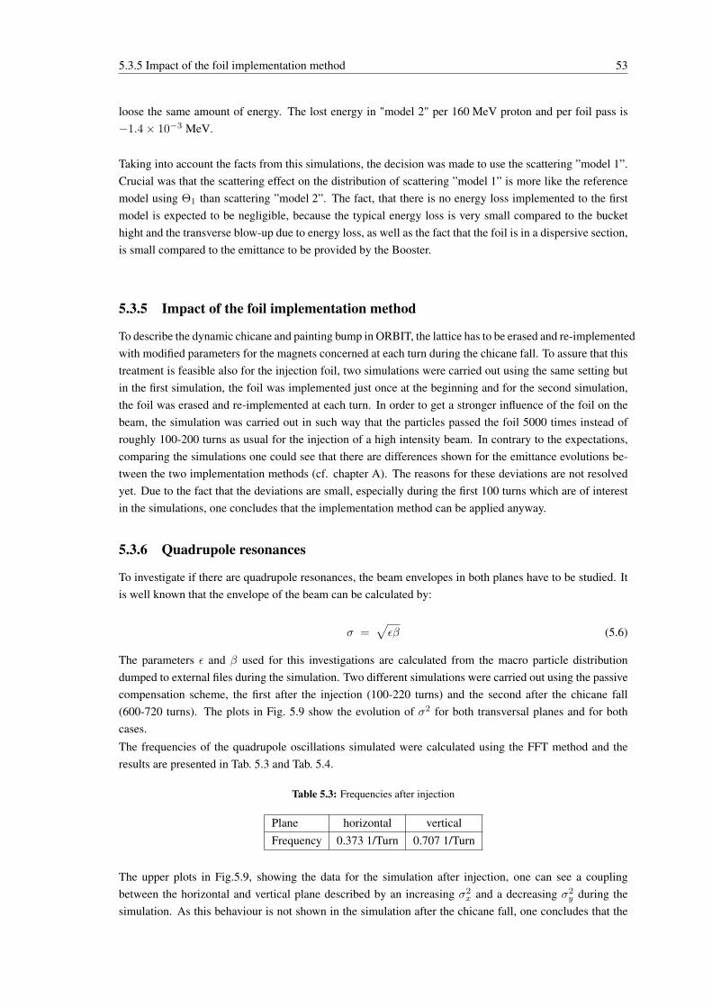
5.3.5 Impact of the foil implementation method 53
loose the same amount of energy. The lost energy in "model 2" per 160 MeV proton and per foil pass is−1.4× 10⁻³ MeV.
Taking into account the facts from this simulations, the decision was made to use the scattering ”model 1”.Crucial was that the scattering effect on the distribution of scattering ”model 1” is more like the referencemodel using Θ1 than scattering ”model 2”. The fact, that there is no energy loss implemented to the firstmodel is expected to be negligible, because the typical energy loss is very small compared to the buckethight and the transverse blow-up due to energy loss, as well as the fact that the foil is in a dispersive section,is small compared to the emittance to be provided by the Booster.
5.3.5 Impact of the foil implementation method
To describe the dynamic chicane and painting bump in ORBIT, the lattice has to be erased and re-implementedwith modified parameters for the magnets concerned at each turn during the chicane fall. To assure that thistreatment is feasible also for the injection foil, two simulations were carried out using the same setting butin the first simulation, the foil was implemented just once at the beginning and for the second simulation,the foil was erased and re-implemented at each turn. In order to get a stronger influence of the foil on thebeam, the simulation was carried out in such way that the particles passed the foil 5000 times instead ofroughly 100-200 turns as usual for the injection of a high intensity beam. In contrary to the expectations,comparing the simulations one could see that there are differences shown for the emittance evolutions be-tween the two implementation methods (cf. chapter A). The reasons for these deviations are not resolvedyet. Due to the fact that the deviations are small, especially during the first 100 turns which are of interestin the simulations, one concludes that the implementation method can be applied anyway.
5.3.6 Quadrupole resonances
To investigate if there are quadrupole resonances, the beam envelopes in both planes have to be studied. Itis well known that the envelope of the beam can be calculated by:
σ =√εβ (5.6)
The parameters ε and β used for this investigations are calculated from the macro particle distributiondumped to external files during the simulation. Two different simulations were carried out using the passivecompensation scheme, the first after the injection (100-220 turns) and the second after the chicane fall(600-720 turns). The plots in Fig. 5.9 show the evolution of σ2 for both transversal planes and for bothcases.
The frequencies of the quadrupole oscillations simulated were calculated using the FFT method and theresults are presented in Tab. 5.3 and Tab. 5.4.
Table 5.3: Frequencies after injection
Plane horizontal verticalFrequency 0.373 1/Turn 0.707 1/Turn
The upper plots in Fig.5.9, showing the data for the simulation after injection, one can see a couplingbetween the horizontal and vertical plane described by an increasing σ2
x and a decreasing σ2y during the
simulation. As this behaviour is not shown in the simulation after the chicane fall, one concludes that the
54 SIMULATIONS
Figure 5.9: σ oscillations. The first line shows the oscillations after the injection and the second line after the chicanefall.
Table 5.4: Frequencies after chicane fall
Plane horizontal verticalFrequency 0.361 1/Turn 0.601 1/Turn
coupling is probably caused by the decreasing chicane, the painting bump or the injection.
Quadrupole resonances in both planes are related to the incoherent space charge tune shift and can becalculated with the following formulas [20]:
Q2,x = 2Q0,x −(
1.5− 0.5ax
ax + ay
)|∆Qinc,x| (5.7)
Q2,y = 2Q0,y −(
1.5− 0.5ay
ax + ay
)|∆Qinc,y| (5.8)
With the frequency of the quadrupole oscillations Q2,x and Q2,y , the frequency of the betatron oscillationsQ0,x and Q0,y , the incoherent tune shifts in both planes ∆Qinc,x and ∆Qinc,y and the horizontal andvertical beam dimensions ax and ay . This formulas were used to calculate the expected tune shift for thegiven quadrupole resonances to compare them with the tune shifts given in the simulations. The expectedvalues are (cf. Fig. 5.18):
∆Qinc,x ≈ −0.35 and ∆Qinc,y ≈ −0.5. (5.9)
The absolute values for the tune shift calculated by the simulated quadrupole resonances are listed inTab. 5.5.
5.3.7 Passive compensation with different pole face rotations 55
Table 5.5: Calculated absolute values for the incoherent tune shift.
Horizontal plane Vertical planeAfter injection 0.31 0.62After chicane fall 0.30 0.47
The values for the incoherent tune shift calculated by the simulated data fits well with the expected tuneshifts for the Booster which explains the frequencies of the quadrupole resonances.
5.3.7 Passive compensation with different pole face rotations
To investigate the impact of the pole face rotations used for the passive compensation on the performanceand to find the best setting, several simulations were carried out using different angles of 0, 20, 40, 50, 60,64, 66 and 70 mrad. The maximum deflection of the beam in the chicane magnets was 66 mrad.
All simulations were run with the same set of macro particles and with the same offset between injected andcirculating beam in both planes. Due to varying focusing effects caused by different pole face rotations, thefall time of the painting bump had to be modified to adjust the horizontal emittance to the required values.Unfortunately, there is no possibility to do such a compensation for the vertical emittance which leads todifferent values. Smaller emittances will lead to less losses during injection and therefore it is necessary totake this effect into account interpreting the data. Table 5.6 shows the normalised emittances after injectionfor all cases. The desired normalised emittances are ε∗x = 12 µm rad and ε∗y = 7 µm rad.
Table 5.6: Normalised emittances after injection for all simulations with different pole face rotations.
0 mrad 20 mrad 40 mrad 50 mrad 60 mrad 64 mrad 66 mrad 70 mradε∗x µm rad 12.04 12.09 12.18 12.20 11.76 12.15 11.93 11.94ε∗y µm rad 6.25 6.54 6.86 6.98 6.97 7.05 7.00 6.39
The vertical emittances for 0, 20 and 70 mrad are much smaller than required. As mentioned above, this willlead to smaller vertical beam sizes (the vertical beta functions are almost the same at the end of injection)and, due to this, to smaller losses during injection. However, these simulations will be compared with theother simulations as well to see what are the effects caused by those angles.
As the fast chicane used for the passive compensation decays between turn 100 and 600, it was sufficientto run this simulations up to 750 turns, because all effects caused by the chicane can be investigated withinthis range. Fig. 5.10 shows the horizontal emittances for all pole face rotations.In the horizontal plane, all emittances are similar at the end of injection due to accordingly modified paint-ing schemes. The different evolutions of these values are caused by different beta functions depending onthe pole face rotations. The smaller the angle of the pole faces, the bigger is the horizontal beta functionand the smaller is the emittance.
In Fig. 5.11, the emittances in the vertical plane are presented. It was not possible to obtain the same valuesfor the vertical emittances at the end of injection for all cases, because there is no vertical painting bump tokeep the emittances at the same values in spite of the different perturbations. The evolution of the verticalemittance during injection is again, like in the horizontal plane, due to the evolution of the beta functions.In vertical plane, the smallest angle of the pole face rotations leads to the smallest beta function and to thebiggest emittance. The data for the horizontal and the vertical beta functions between injection and up to
56 SIMULATIONS
750 turns are presented on the right hand side in Fig. 5.12.
The emittance evolution in the vertical plane after injection is almost the same for the angles between 60-70mrad. For the smaller angles below 60 mrad, the emittances are shrinking due to more particle losses causedby the not compensated part of the perturbations.
Fig. 5.13 shows the loss rates per turn for all different pole face rotations. There are losses during injectioncaused by the used linear decreasing painting bump. The losses for the simulations with angels between60 and 70 mrad are much smaller than the loss rates for pole face rotations below 60 mrad. Due to this,the best setting has to be found within this range. More information about the losses are provided in theplots for the accumulated losses shown in Fig. 5.14. The one on the left shows clearly that out of the set ofangles up to 50 mrad, the 50 mrad pole face rotation leads to the smallest number of losses. In the plots onthe right hand side, the number of lost particles for a pole face rotation of 70 mrad is the smallest. This isa surprisingly result, because a 70 mrad angle is already over compensation for a maximum deflection of66 mrad. Probably this result is caused by another effect which was not taken into account. One possibilityis that the normalised emittance for the 70 mrad pole face rotation was smaller than for other angles. Thisleads to a smaller beam size and possibly to less losses. Also the the emittances for the 66 mrad case, whichshows also a relative low loss rate, was smaller then the nominal value. However, the emittance for the 64mrad case was bigger than the desired values in both planes and the accumulated losses are in the samerange as for the 66 mrad pole face rotation. This fact leaded to the decision to use the 64 mrad pole facerotation for further simulations.
Tab. 5.7 shows the particle losses in percentage of the beam for simulations with different pole face rota-tions. The first line presents the numbers of losses for all turns up to 750, the second line the losses duringinjection and the third line all losses between the end of injection and 750 turns.
Table 5.7: The loss rate for different pole face rotations in percentage of the beam for the injection, for the time afterthe injection and for the whole time of the simulation.
0 mrad 20 mrad 40 mrad 50 mrad 60 mrad 64 mrad 66 mrad 70 mradAll 25.02 % 16.30 % 9.26 % 6.59 % 4.16 % 4.20 % 4.00 % 3.43 %
Injection 17.64 % 12.15 % 6.92 % 4.44 % 2.04 % 1.57 % 1.25 % 0.76 %After Injection 7.39 % 4.16 % 2.34 % 2.15 % 2.12 % 2.63 % 2.75 % 2.67 %
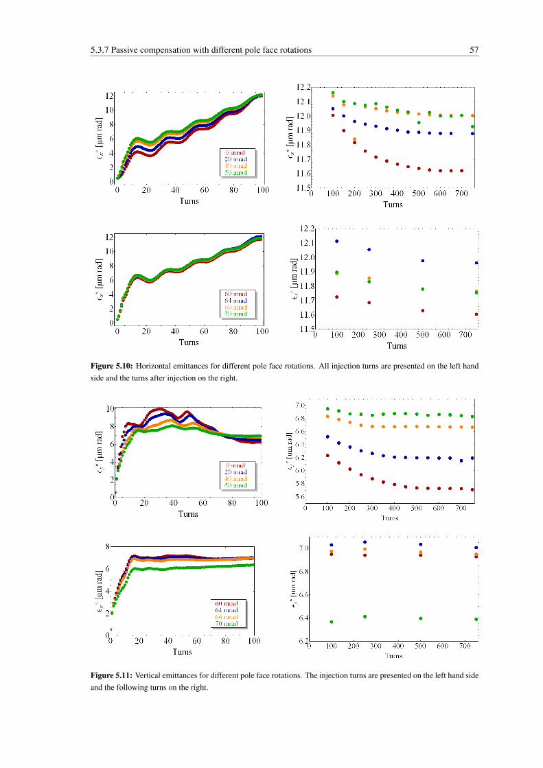
5.3.7 Passive compensation with different pole face rotations 57
Figure 5.10: Horizontal emittances for different pole face rotations. All injection turns are presented on the left handside and the turns after injection on the right.
Figure 5.11: Vertical emittances for different pole face rotations. The injection turns are presented on the left hand sideand the following turns on the right.
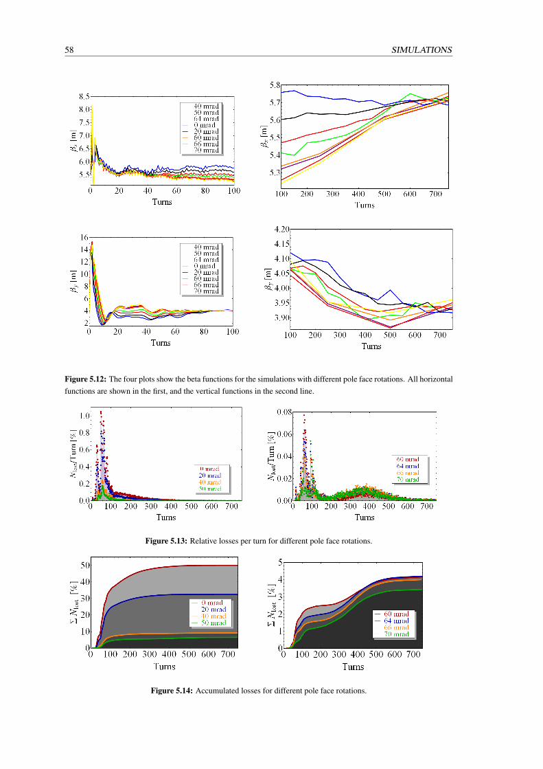
58 SIMULATIONS
Figure 5.12: The four plots show the beta functions for the simulations with different pole face rotations. All horizontalfunctions are shown in the first, and the vertical functions in the second line.
Figure 5.13: Relative losses per turn for different pole face rotations.
Figure 5.14: Accumulated losses for different pole face rotations.
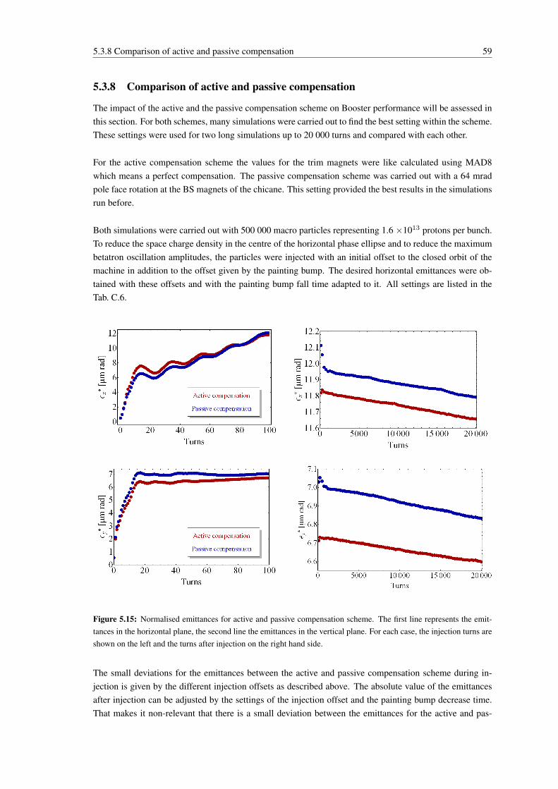
5.3.8 Comparison of active and passive compensation 59
5.3.8 Comparison of active and passive compensation
The impact of the active and the passive compensation scheme on Booster performance will be assessed inthis section. For both schemes, many simulations were carried out to find the best setting within the scheme.These settings were used for two long simulations up to 20 000 turns and compared with each other.
For the active compensation scheme the values for the trim magnets were like calculated using MAD8which means a perfect compensation. The passive compensation scheme was carried out with a 64 mradpole face rotation at the BS magnets of the chicane. This setting provided the best results in the simulationsrun before.
Both simulations were carried out with 500 000 macro particles representing 1.6 ×10¹³ protons per bunch.To reduce the space charge density in the centre of the horizontal phase ellipse and to reduce the maximumbetatron oscillation amplitudes, the particles were injected with an initial offset to the closed orbit of themachine in addition to the offset given by the painting bump. The desired horizontal emittances were ob-tained with these offsets and with the painting bump fall time adapted to it. All settings are listed in theTab. C.6.
Figure 5.15: Normalised emittances for active and passive compensation scheme. The first line represents the emit-tances in the horizontal plane, the second line the emittances in the vertical plane. For each case, the injection turns areshown on the left and the turns after injection on the right hand side.
The small deviations for the emittances between the active and passive compensation scheme during in-jection is given by the different injection offsets as described above. The absolute value of the emittancesafter injection can be adjusted by the settings of the injection offset and the painting bump decrease time.That makes it non-relevant that there is a small deviation between the emittances for the active and pas-
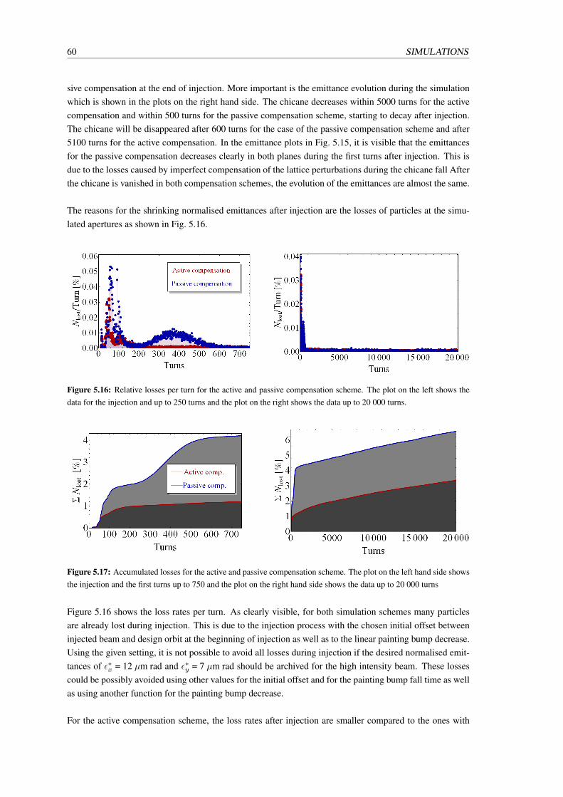
60 SIMULATIONS
sive compensation at the end of injection. More important is the emittance evolution during the simulationwhich is shown in the plots on the right hand side. The chicane decreases within 5000 turns for the activecompensation and within 500 turns for the passive compensation scheme, starting to decay after injection.The chicane will be disappeared after 600 turns for the case of the passive compensation scheme and after5100 turns for the active compensation. In the emittance plots in Fig. 5.15, it is visible that the emittancesfor the passive compensation decreases clearly in both planes during the first turns after injection. This isdue to the losses caused by imperfect compensation of the lattice perturbations during the chicane fall Afterthe chicane is vanished in both compensation schemes, the evolution of the emittances are almost the same.
The reasons for the shrinking normalised emittances after injection are the losses of particles at the simu-lated apertures as shown in Fig. 5.16.
Figure 5.16: Relative losses per turn for the active and passive compensation scheme. The plot on the left shows thedata for the injection and up to 250 turns and the plot on the right shows the data up to 20 000 turns.
Figure 5.17: Accumulated losses for the active and passive compensation scheme. The plot on the left hand side showsthe injection and the first turns up to 750 and the plot on the right hand side shows the data up to 20 000 turns
Figure 5.16 shows the loss rates per turn. As clearly visible, for both simulation schemes many particlesare already lost during injection. This is due to the injection process with the chosen initial offset betweeninjected beam and design orbit at the beginning of injection as well as to the linear painting bump decrease.Using the given setting, it is not possible to avoid all losses during injection if the desired normalised emit-tances of ε∗x = 12 µm rad and ε∗y = 7 µm rad should be archived for the high intensity beam. These lossescould be possibly avoided using other values for the initial offset and for the painting bump fall time as wellas using another function for the painting bump decrease.
For the active compensation scheme, the loss rates after injection are smaller compared to the ones with
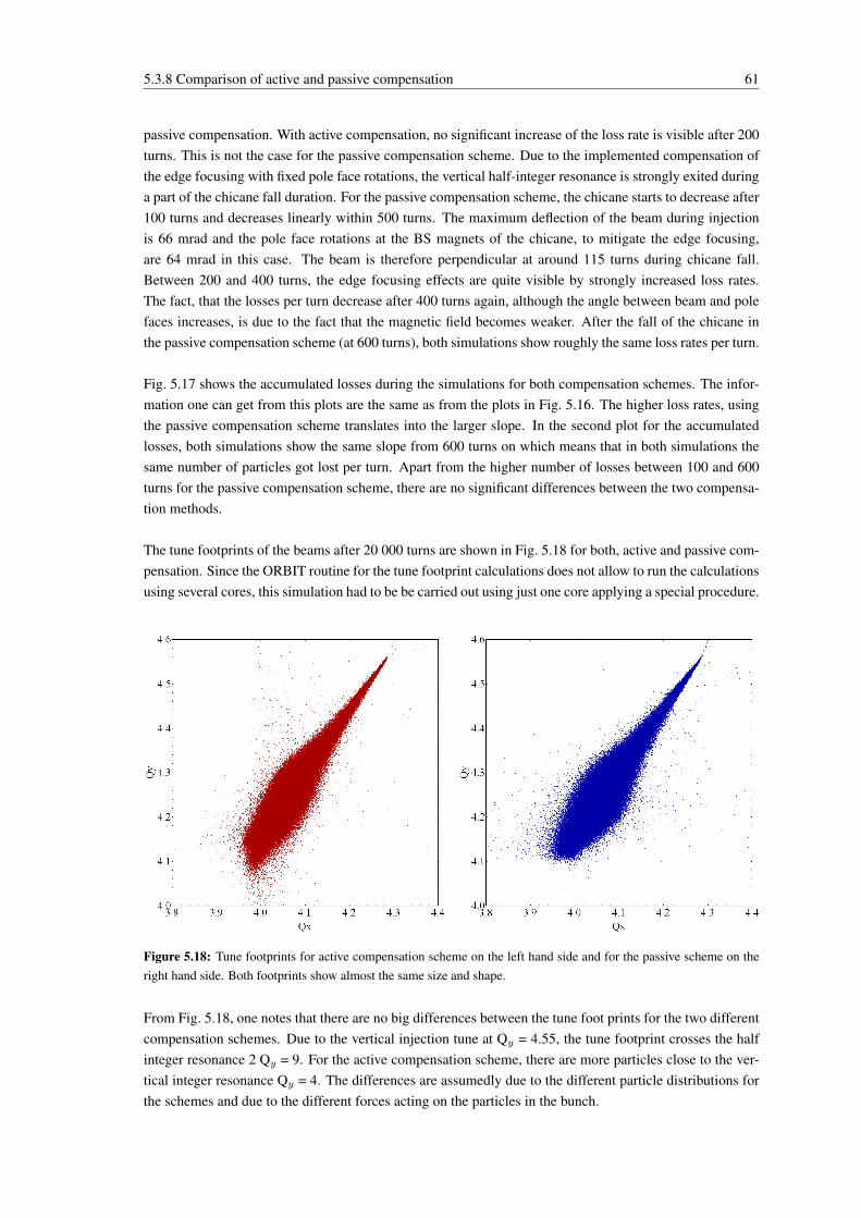
5.3.8 Comparison of active and passive compensation 61
passive compensation. With active compensation, no significant increase of the loss rate is visible after 200turns. This is not the case for the passive compensation scheme. Due to the implemented compensation ofthe edge focusing with fixed pole face rotations, the vertical half-integer resonance is strongly exited duringa part of the chicane fall duration. For the passive compensation scheme, the chicane starts to decrease after100 turns and decreases linearly within 500 turns. The maximum deflection of the beam during injectionis 66 mrad and the pole face rotations at the BS magnets of the chicane, to mitigate the edge focusing,are 64 mrad in this case. The beam is therefore perpendicular at around 115 turns during chicane fall.Between 200 and 400 turns, the edge focusing effects are quite visible by strongly increased loss rates.The fact, that the losses per turn decrease after 400 turns again, although the angle between beam and polefaces increases, is due to the fact that the magnetic field becomes weaker. After the fall of the chicane inthe passive compensation scheme (at 600 turns), both simulations show roughly the same loss rates per turn.
Fig. 5.17 shows the accumulated losses during the simulations for both compensation schemes. The infor-mation one can get from this plots are the same as from the plots in Fig. 5.16. The higher loss rates, usingthe passive compensation scheme translates into the larger slope. In the second plot for the accumulatedlosses, both simulations show the same slope from 600 turns on which means that in both simulations thesame number of particles got lost per turn. Apart from the higher number of losses between 100 and 600turns for the passive compensation scheme, there are no significant differences between the two compensa-tion methods.
The tune footprints of the beams after 20 000 turns are shown in Fig. 5.18 for both, active and passive com-pensation. Since the ORBIT routine for the tune footprint calculations does not allow to run the calculationsusing several cores, this simulation had to be be carried out using just one core applying a special procedure.
Figure 5.18: Tune footprints for active compensation scheme on the left hand side and for the passive scheme on theright hand side. Both footprints show almost the same size and shape.
From Fig. 5.18, one notes that there are no big differences between the tune foot prints for the two differentcompensation schemes. Due to the vertical injection tune at Qy = 4.55, the tune footprint crosses the halfinteger resonance 2 Qy = 9. For the active compensation scheme, there are more particles close to the ver-tical integer resonance Qy = 4. The differences are assumedly due to the different particle distributions forthe schemes and due to the different forces acting on the particles in the bunch.
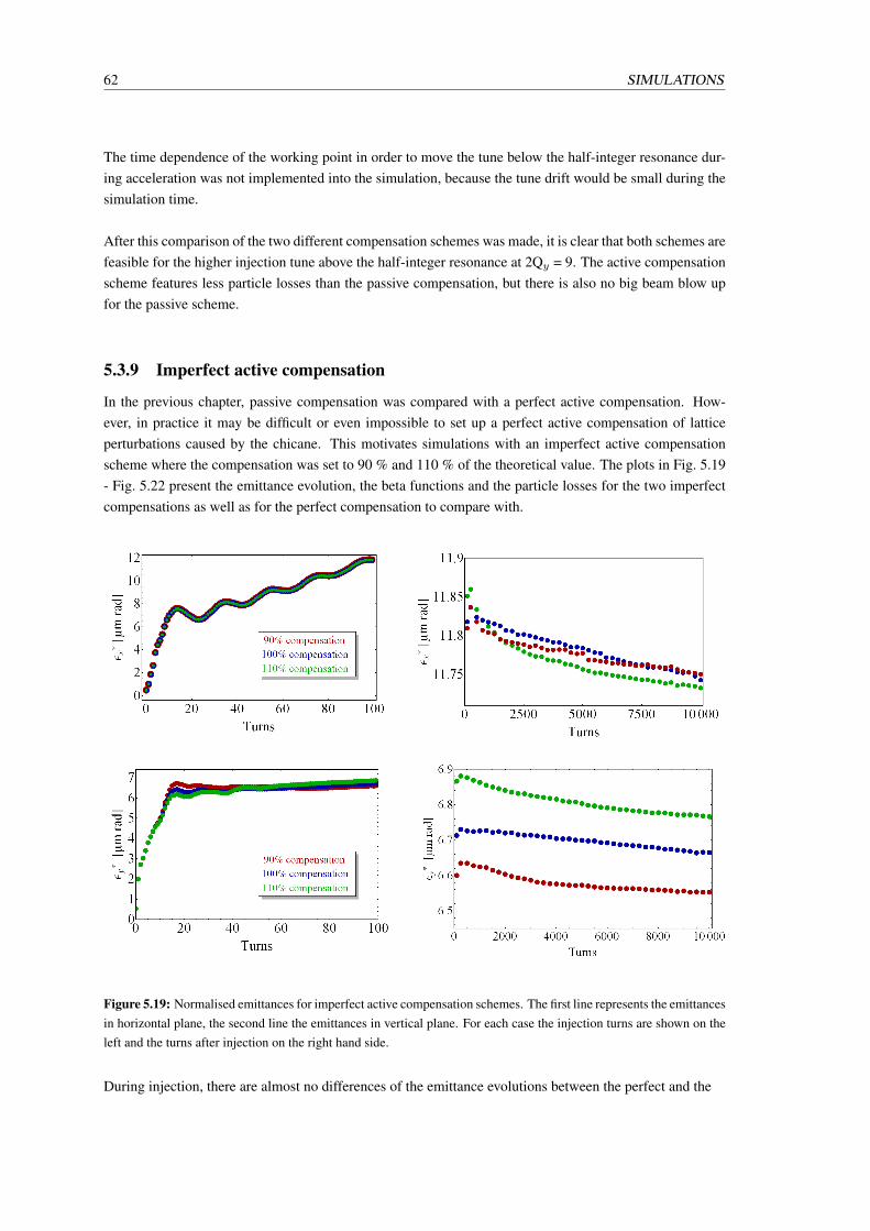
62 SIMULATIONS
The time dependence of the working point in order to move the tune below the half-integer resonance dur-ing acceleration was not implemented into the simulation, because the tune drift would be small during thesimulation time.
After this comparison of the two different compensation schemes was made, it is clear that both schemes arefeasible for the higher injection tune above the half-integer resonance at 2Qy = 9. The active compensationscheme features less particle losses than the passive compensation, but there is also no big beam blow upfor the passive scheme.
5.3.9 Imperfect active compensation
In the previous chapter, passive compensation was compared with a perfect active compensation. How-ever, in practice it may be difficult or even impossible to set up a perfect active compensation of latticeperturbations caused by the chicane. This motivates simulations with an imperfect active compensationscheme where the compensation was set to 90 % and 110 % of the theoretical value. The plots in Fig. 5.19- Fig. 5.22 present the emittance evolution, the beta functions and the particle losses for the two imperfectcompensations as well as for the perfect compensation to compare with.
Figure 5.19: Normalised emittances for imperfect active compensation schemes. The first line represents the emittancesin horizontal plane, the second line the emittances in vertical plane. For each case the injection turns are shown on theleft and the turns after injection on the right hand side.
During injection, there are almost no differences of the emittance evolutions between the perfect and the
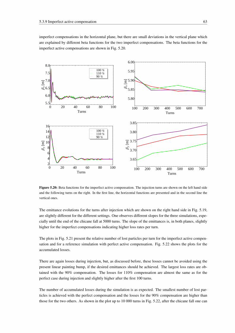
5.3.9 Imperfect active compensation 63
imperfect compensations in the horizontal plane, but there are small deviations in the vertical plane whichare explained by different beta functions for the two imperfect compensations. The beta functions for theimperfect active compensations are shown in Fig. 5.20.
0 20 40 60 80 1005.5
6.0
6.5
7.0
7.5
8.0
Turns
Βx
@mD 90 %
110 %100 %
100 200 300 400 500 600 700
5.80
5.85
5.90
5.95
6.00
Turns
Βx
@mD
0 20 40 60 80 1002
4
6
8
10
12
14
16
Turns
Βy
@mD 90 %
110 %100 %
100 200 300 400 500 600 700
3.65
3.70
3.75
3.80
3.85
Turns
Βy
@mD
Figure 5.20: Beta functions for the imperfect active compensation. The injection turns are shown on the left hand sideand the following turns on the right. In the first line, the horizontal functions are presented and in the second line thevertical ones.
The emittance evolutions for the turns after injection which are shown on the right hand side in Fig. 5.19,are slightly different for the different settings. One observes different slopes for the three simulations, espe-cially until the end of the chicane fall at 5000 turns. The slope of the emittances is, in both planes, slightlyhigher for the imperfect compensations indicating higher loss rates per turn.
The plots in Fig. 5.21 present the relative number of lost particles per turn for the imperfect active compen-sation and for a reference simulation with perfect active compensation. Fig. 5.22 shows the plots for theaccumulated losses.
There are again losses during injection, but, as discussed before, these losses cannot be avoided using thepresent linear painting bump, if the desired emittances should be achieved. The largest loss rates are ob-tained with the 90% compensation. The losses for 110% compensation are almost the same as for theperfect case during injection and slightly higher after the first 100 turns.
The number of accumulated losses during the simulation is as expected. The smallest number of lost par-ticles is achieved with the perfect compensation and the losses for the 90% compensation are higher thanthose for the two others. As shown in the plot up to 10 000 turns in Fig. 5.22, after the chicane fall one can
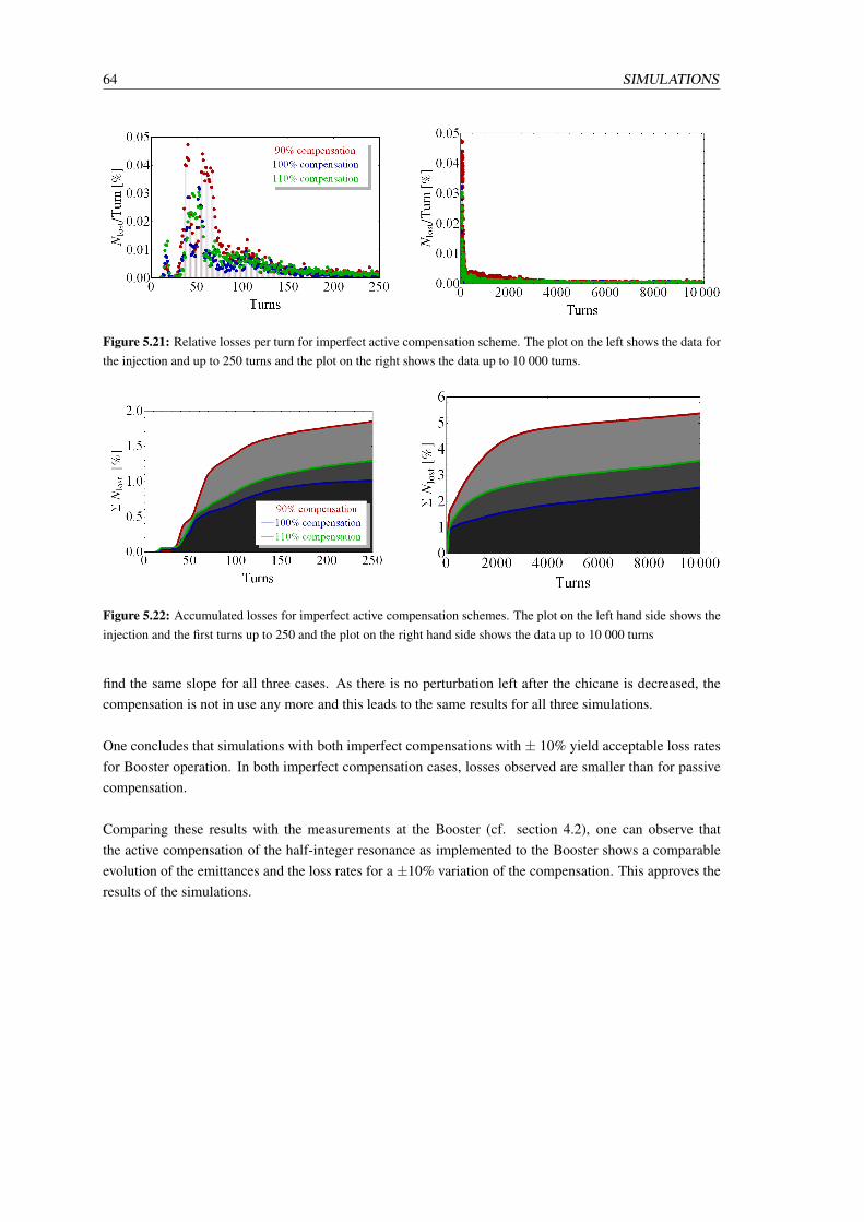
64 SIMULATIONS
Figure 5.21: Relative losses per turn for imperfect active compensation scheme. The plot on the left shows the data forthe injection and up to 250 turns and the plot on the right shows the data up to 10 000 turns.
Figure 5.22: Accumulated losses for imperfect active compensation schemes. The plot on the left hand side shows theinjection and the first turns up to 250 and the plot on the right hand side shows the data up to 10 000 turns
find the same slope for all three cases. As there is no perturbation left after the chicane is decreased, thecompensation is not in use any more and this leads to the same results for all three simulations.
One concludes that simulations with both imperfect compensations with ± 10% yield acceptable loss ratesfor Booster operation. In both imperfect compensation cases, losses observed are smaller than for passivecompensation.
Comparing these results with the measurements at the Booster (cf. section 4.2), one can observe thatthe active compensation of the half-integer resonance as implemented to the Booster shows a comparableevolution of the emittances and the loss rates for a ±10% variation of the compensation. This approves theresults of the simulations.
Chapter 6
Conclusions and prospects
The most important conclusion of the simulations presented in this thesis is that the injection of a highintensity beam from Linac4 to the PS Booster and the acceleration of the particles is feasible with bothcompensation schemes for the higher vertical tune above the half integer resonance at 2Qy = 9.
Furthermore, the single simulations and the comparison of the data led to the following conclusions:
• The first test were concerning to basic implementations to the ORBIT code like the accelerationfunction. Testing the impact of this tool, one could see that the acceleration is well implemented tothe code.
• The apertures are implemented with dimensions corresponding to the PS Booster as existing at themoment and the size of the beam scope window is adapted to the higher injection energy with Linac4.An additional aperture was implemented to the injection area to simulate the injection septum at thesecond chicane magnet. A test simulation showed that the apertures are implemented properly.
• The benchmarking on the number of macro particles showed that 500 000 macro particles are enoughto avoid statistical effects and the size of the dumped files are still in a rage one can handle.
• The comparison of the different foil scattering models implemented to ORBIT led to the decisionto use scattering "model 1" which represents the expected scattering distribution much better than"model 2". It was decided that the disregard of the energy loss for scattered particles in "model 1"can be neglected due to the fact that the expected effects are small.
• To simulate the dynamic chicane in the injection area running ORBIT simulations, the lattice elementshave to be erased and reinstalled each turn during the chicane fall. The simulation to investigateimpacts caused by the continuously re-installation of the foil showed unexpected deviations betweenthe simulations with a lattice which was installed just once and a lattice which was reinstalled duringeach turn. The reasons for the deviations were not completely understood and it may be interestingto continue with further investigation on this topic.
• The quadrupole resonances documented for one simulation applying the passive compensation schemeshow the frequencies which were expected due to the fact that those frequencies are related to the tunespread.
• Simulating the passive compensation scheme for the perturbations at the chicane magnets, one inves-tigated that it is feasible to run the machine applying this compensation method. A benchmarking onthe pole face rotations aiming to find the angle which leads to the smallest particle losses led to the
66 CHAPTER 6. CONCLUSIONS AND PROSPECTS
surprisingly large angle of 64 mrad. Further studies could confirm this value and one could run addi-tional simulations to explore the best pole face rotation angle for other beams like the LHC nominalbeam.
• Running simulations for both compensation schemes and comparing the results, one could find outthat the active compensation scheme leads to less losses than the passive one. Both compensationschemes show losses during the injection which are related to the fact that some particles are alreadyinjected outside the machine acceptance. This was not avoidable using a linear painting bump ifthe required emittances for a high intensity beam should be achieved. One possibility to reducethe number of lost particles during injection is eventually to modify the function of the paintingbump. Further losses occurred in case of the passive compensation during the chicane fall causedby the fact that the compensation of the edge focusing effects cannot be realised with a fixed passivecompensation during the whole fall of the chicane. The losses during the chicane fall plus the lossesduring injection lead to higher loss rates for the passive compensation compared with the activecounterpart, but still the losses for both schemes are in an acceptable range.
• The simulation treating a perfect active compensation demonstrated the feasibility of the scheme, butit was also of note to see the results for an imperfect active compensation. Two simulations with± 10 % variation of the compensation magnet strength showed that the loss rates are higher than forthe perfect case, but still acceptable. The simulation for the 110 % focusing strength in the trims ledto roughly 30 % more losses and the 90 % focusing strength doubled the number of lost particlescompared to the perfect compensation.
Due to different fall times of the chicane for the two compensation schemes, there are also different re-quirements on the lattice elements. Both schemes have different demands on the power supplies, the activecompensation scheme for the additional trim magnets which have to follow a pre-programmed time evo-lution in order to compensate the varying edge focusing effects during the chicane fall, and the passivecompensation needs fast and powerful power supplies to realise the chicane fall within 0.5 ms. The fastchicane applied for the passive compensation scheme requires also special vacuum chambers, otherwise,the fast ramped magnets will induce currents which will then lead to further perturbations. This problemscan be solved with ceramic vacuum chambers. Eventually, the ceramic vacuum chambers or corrugatedvacuum chambers have to be used also with the active compensation. One should also consider, that thepassive compensation scheme will be fixed whereas the active compensation will be flexible which couldbe once an advantage if something will be changed in the Booster lattice or in the operating schedule.
A further tasks concerning the simulations of the H− charge exchange injection from Linac4 to the Boostercould be the implementation of imperfections caused by additional multipolar components and misalign-ment of lattice elements in order to investigate the impact of these perturbations on the Booster performance.
Furthermore, it could be interesting to get a modified ORBIT code which gives the possibility to changethe strength of quadrupole and dipole magnets in order to realise the dynamic lattice without erasing andreinstalling the lattice at each turn. Another useful implementation would be a function to calculate theemittances and other beam parameters in ORBIT without dumping the particle coordinates which requiresa lot of memory space and time for the calculation.
Appendix A
Deviations due to the re-installation ofthe lattice
During the chicane fall, the lattice has to be erased and re-implemented at each turn with modified valuesfor the magnets related to the chicane and, in case of the active compensation, for the magnets related to thetrim quadrupols. No artefacts were expected with this procedure [21]. Nevertheless, to investigate if thereare unusual impacts from the fact that the lattice, and especially the foil, is reinstalled at each turn, twosimulations were carried out and compared. The two runs started for this comparison were exactly the samebut in the first one, the lattice was installed just once at the beginning and in the second run, the installationtook place at each turn.
The used lattice was fixed which means without decaying bumps. Thus, there are no disturbing factors bychicane modifications and the beam passed through the foil during the whole simulation and not just forthe injection turns. This will enlarge the effect of the foil on the beam and, if there are differences betweenthe two ways to install the lattice, they will be more developed. The desired emittances were archived byan offset in both planes between the injected beam and the design orbit. To speed up the simulations, theywere run with 100 000 macro particles instead of half a million like usual. This should be no problem,because the reason to run this simulations is just to find differences between the two simulations if existing.If there is any impact caused by the smaller number of macro particles, it will occur in both simulations. Allsimulation settings are summarised in Tab. C.3. The plots in Fig. A.1 show the emittance evolution duringthe simulation.
The emittance evolution is the same for both simulations during injection. After the injection and due toscattering at the injection foil, there is an emittances growth up to approximately 300 turns in both planesand for both simulations. After the beam reaches a certain size, more and more particles get lost at theapertures and the emittance starts to shrink again. Small deviations between the two injection schemes takeplace for higher turn numbers which was not expected. The reasons for the different result are not clear yetand have to be investigated later.
One notes that the accumulated losses for the two simulations, presented in Fig. A.2, are almost identical.From this observation and the almost similar emittance evolutions during the injection, one concludes thatthe procedure with regular re-installation of the lattice has negligible impact on the results of the simulation.
67
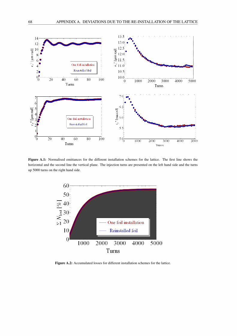
68 APPENDIX A. DEVIATIONS DUE TO THE RE-INSTALLATION OF THE LATTICE
Figure A.1: Normalised emittances for the different installation schemes for the lattice. The first line shows thehorizontal and the second line the vertical plane. The injection turns are presented on the left hand side and the turnsup 5000 turns on the right hand side.
Figure A.2: Accumulated losses for different installation schemes for the lattice.

Appendix B
Measurements at the PS Booster
All data of the emittance measurements at the PS Booster (cf. chapter 4), are listed in the following Tab. B.1.
69
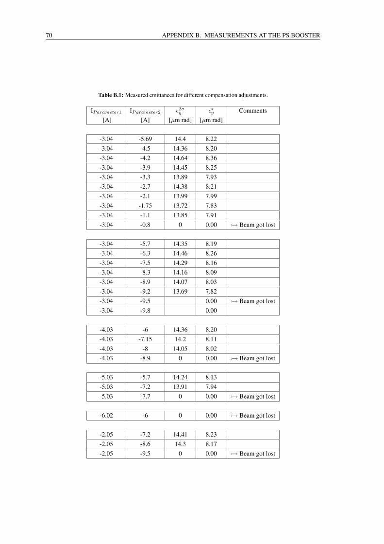
70 APPENDIX B. MEASUREMENTS AT THE PS BOOSTER
Table B.1: Measured emittances for different compensation adjustments.
IParameter1 IParameter2 ε2σy ε∗y Comments[A] [A] [µm rad] [µm rad]
-3.04 -5.69 14.4 8.22-3.04 -4.5 14.36 8.20-3.04 -4.2 14.64 8.36-3.04 -3.9 14.45 8.25-3.04 -3.3 13.89 7.93-3.04 -2.7 14.38 8.21-3.04 -2.1 13.99 7.99-3.04 -1.75 13.72 7.83-3.04 -1.1 13.85 7.91-3.04 -0.8 0 0.00 Beam got lost
-3.04 -5.7 14.35 8.19-3.04 -6.3 14.46 8.26-3.04 -7.5 14.29 8.16-3.04 -8.3 14.16 8.09-3.04 -8.9 14.07 8.03-3.04 -9.2 13.69 7.82-3.04 -9.5 0.00 Beam got lost-3.04 -9.8 0.00
-4.03 -6 14.36 8.20-4.03 -7.15 14.2 8.11-4.03 -8 14.05 8.02-4.03 -8.9 0 0.00 Beam got lost
-5.03 -5.7 14.24 8.13-5.03 -7.2 13.91 7.94-5.03 -7.7 0 0.00 Beam got lost
-6.02 -6 0 0.00 Beam got lost
-2.05 -7.2 14.41 8.23-2.05 -8.6 14.3 8.17-2.05 -9.5 0 0.00 Beam got lost

Appendix C
Simulation settings
In the following tables, one can find all settings used for the simulations presented in chapter 5.
71
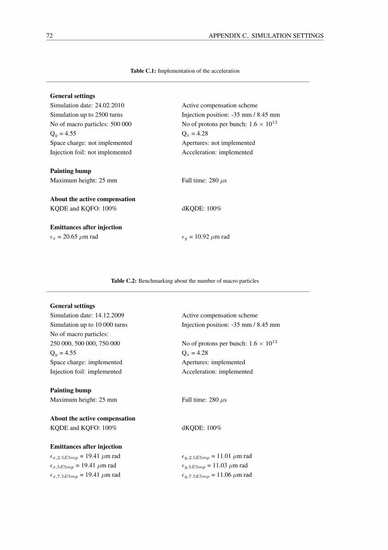
72 APPENDIX C. SIMULATION SETTINGS
Table C.1: Implementation of the acceleration
General settingsSimulation date: 24.02.2010 Active compensation schemeSimulation up to 2500 turns Injection position: -35 mm / 8.45 mmNo of macro particles: 500 000 No of protons per bunch: 1.6 × 10¹³
Qy = 4.55 Qx = 4.28Space charge: not implemented Apertures: not implementedInjection foil: not implemented Acceleration: implemented
Painting bumpMaximum height: 25 mm Fall time: 280 µs
About the active compensationKQDE and KQFO: 100% dKQDE: 100%
Emittances after injectionεx = 20.65 µm rad εy = 10.92 µm rad
Table C.2: Benchmarking about the number of macro particles
General settingsSimulation date: 14.12.2009 Active compensation schemeSimulation up to 10 000 turns Injection position: -35 mm / 8.45 mmNo of macro particles:250 000, 500 000, 750 000 No of protons per bunch: 1.6 × 10¹³
Qy = 4.55 Qx = 4.28Space charge: implemented Apertures: implementedInjection foil: implemented Acceleration: implemented
Painting bumpMaximum height: 25 mm Fall time: 280 µs
About the active compensationKQDE and KQFO: 100% dKQDE: 100%
Emittances after injectionεx,2.5E5mp = 19.41 µm rad εy,2.5E5mp = 11.01 µm radεx,5E5mp = 19.41 µm rad εy,5E5mp = 11.03 µm radεx,7.5E5mp = 19.41 µm rad εy,7.5E5mp = 11.06 µm rad

73
Table C.3: Simulations to investigate deviations caused by the re-installation of the stripping foil.
General settingsSimulation date: 10.05.2010 Active compensation schemeSimulation up to 10 000 turns Injection position: -14.95 mm / 8.45 mmNo of macro particles: 100 000 No of protons per bunch: 1.6 × 10¹³
Qy = 4.55 Qx = 4.28Space charge: implemented Apertures: implementedInjection foil: implemented Acceleration: implemented
Painting bumpA fixed lattice without painting bump was used
About the active compensationKQDE and KQFO: 100% dKQDE: 100%
Emittances after injectionεx,one implementation = 20.12 µm rad εy,one implementation = 11.04 µm radεx,reimplementation = 20.12 µm rad εy,reimplementation = 11.04 µm rad
Table C.4: Investigation of quadrupole resonances after injection and after chicane fall.
General settingsSimulation date: 19.02.2010 Passive compensation schemeSimulation up to 220 respectively to 720 turns Injection position: -14.95 mm / 8.45 mmNo of macro particles: 100 000 No of protons per bunch: 1.6 × 10¹³
Qy = 4.55 Qx = 4.28Space charge: implemented Apertures: implementedInjection foil: implemented Acceleration: implemented
Painting bumpA fixed lattice without painting bump was used
About the passive compensationPole face rotation: 64 mrad
Emittances after injectionεx = 19.90 µm rad εy = 11.55 µm rad
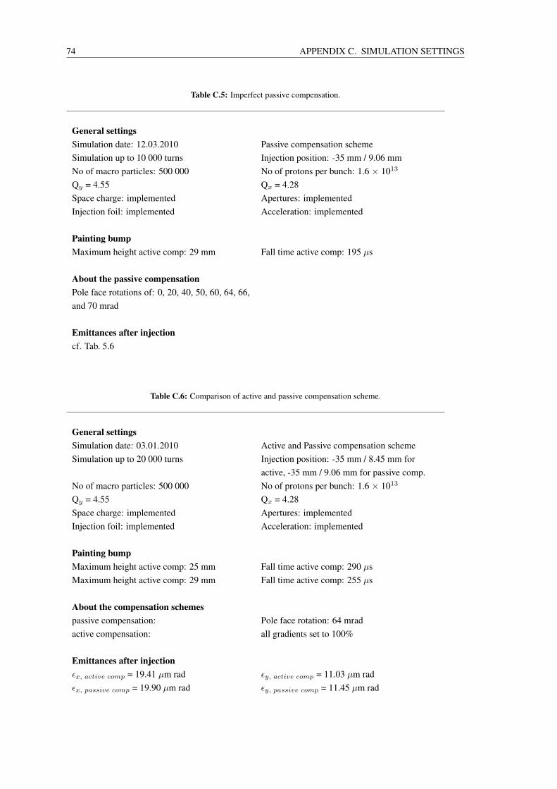
74 APPENDIX C. SIMULATION SETTINGS
Table C.5: Imperfect passive compensation.
General settingsSimulation date: 12.03.2010 Passive compensation schemeSimulation up to 10 000 turns Injection position: -35 mm / 9.06 mmNo of macro particles: 500 000 No of protons per bunch: 1.6 × 10¹³
Qy = 4.55 Qx = 4.28Space charge: implemented Apertures: implementedInjection foil: implemented Acceleration: implemented
Painting bumpMaximum height active comp: 29 mm Fall time active comp: 195 µs
About the passive compensationPole face rotations of: 0, 20, 40, 50, 60, 64, 66,and 70 mrad
Emittances after injectioncf. Tab. 5.6
Table C.6: Comparison of active and passive compensation scheme.
General settingsSimulation date: 03.01.2010 Active and Passive compensation schemeSimulation up to 20 000 turns Injection position: -35 mm / 8.45 mm for
active, -35 mm / 9.06 mm for passive comp.No of macro particles: 500 000 No of protons per bunch: 1.6 × 10¹³
Qy = 4.55 Qx = 4.28Space charge: implemented Apertures: implementedInjection foil: implemented Acceleration: implemented
Painting bumpMaximum height active comp: 25 mm Fall time active comp: 290 µsMaximum height active comp: 29 mm Fall time active comp: 255 µs
About the compensation schemespassive compensation: Pole face rotation: 64 mradactive compensation: all gradients set to 100%
Emittances after injectionεx, active comp = 19.41 µm rad εy, active comp = 11.03 µm radεx, passive comp = 19.90 µm rad εy, passive comp = 11.45 µm rad
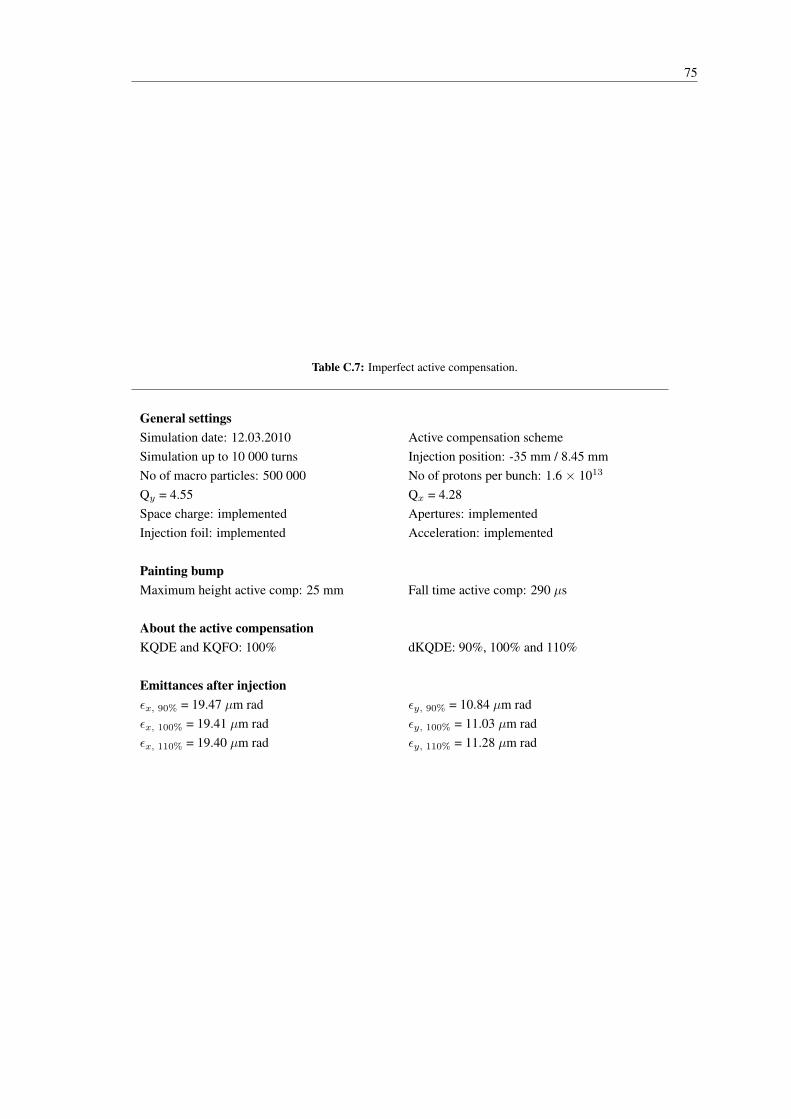
75
Table C.7: Imperfect active compensation.
General settingsSimulation date: 12.03.2010 Active compensation schemeSimulation up to 10 000 turns Injection position: -35 mm / 8.45 mmNo of macro particles: 500 000 No of protons per bunch: 1.6 × 10¹³
Qy = 4.55 Qx = 4.28Space charge: implemented Apertures: implementedInjection foil: implemented Acceleration: implemented
Painting bumpMaximum height active comp: 25 mm Fall time active comp: 290 µs
About the active compensationKQDE and KQFO: 100% dKQDE: 90%, 100% and 110%
Emittances after injectionεx, 90% = 19.47 µm rad εy, 90% = 10.84 µm radεx, 100% = 19.41 µm rad εy, 100% = 11.03 µm radεx, 110% = 19.40 µm rad εy, 110% = 11.28 µm rad

76 APPENDIX C. SIMULATION SETTINGS

List of Figures
1.1 All Accelerators at CERN [?]. . . . . . . . . . . . . . . . . . . . . . . . . . . . . . . . . 1
2.1 Used Coordinate system . . . . . . . . . . . . . . . . . . . . . . . . . . . . . . . . . . . 32.2 Phase ellipse. . . . . . . . . . . . . . . . . . . . . . . . . . . . . . . . . . . . . . . . . . 82.3 Edge focusing. . . . . . . . . . . . . . . . . . . . . . . . . . . . . . . . . . . . . . . . . 102.4 Horizontal painting. . . . . . . . . . . . . . . . . . . . . . . . . . . . . . . . . . . . . . . 112.5 RF wave and bucket. . . . . . . . . . . . . . . . . . . . . . . . . . . . . . . . . . . . . . 142.6 Impact of the acceleration on the particles velocity. . . . . . . . . . . . . . . . . . . . . . 142.7 Longitudinal painting. [7]. . . . . . . . . . . . . . . . . . . . . . . . . . . . . . . . . . . 152.8 Schematic drawing of a cylindrical bunch. . . . . . . . . . . . . . . . . . . . . . . . . . . 162.9 Emittance measurement in the normalised phase space. . . . . . . . . . . . . . . . . . . . 19
3.1 Proton Synchrotron Booster layout [11]. . . . . . . . . . . . . . . . . . . . . . . . . . . . 213.2 Regular period of the PS Booster. . . . . . . . . . . . . . . . . . . . . . . . . . . . . . . . 223.3 Flatted bucket of the applied double harmonic system [7]. Date: 14.04.2010 . . . . . . . . 223.4 Tune footprint for active compensation scheme after 5000 turns. Date: 03.01.2010 . . . . . 233.5 Injection and ejection elements. . . . . . . . . . . . . . . . . . . . . . . . . . . . . . . . 253.6 Sketch of the injection from Linac2 to PS Booster [11]. . . . . . . . . . . . . . . . . . . . 263.7 Sketch of the Booster ejection as used with Linac2 [11]. . . . . . . . . . . . . . . . . . . . 273.8 Multi turn injection. . . . . . . . . . . . . . . . . . . . . . . . . . . . . . . . . . . . . . . 283.9 Structure of Linac4 [14]. . . . . . . . . . . . . . . . . . . . . . . . . . . . . . . . . . . . 293.10 Scheme of the distributor and septum magnets [14]. . . . . . . . . . . . . . . . . . . . . . 303.11 Scheme of a H− charge exchange injection [14]. . . . . . . . . . . . . . . . . . . . . . . . 313.12 Movement of the bunches in horizontal phase space for the H− injection. . . . . . . . . . 313.13 Passive compensation scheme with pole face rotations. . . . . . . . . . . . . . . . . . . . 333.14 Elements of the Booster measurement line [14]. . . . . . . . . . . . . . . . . . . . . . . . 33
4.1 Tomoscope acquisition for a CNGS beam. Date: 14.12.2009 . . . . . . . . . . . . . . . . 364.2 Tomoscope reconstruction. Date: 14.12.2009 . . . . . . . . . . . . . . . . . . . . . . . . 364.3 Horizontal emittance measurement for a CNGS beam at the Booster. Date: 14.12.2009 . . 374.4 Overview of all measurements of the compensation sensitivity of the Booster. Date: 16.11.2009 394.5 Measured emittances for different compensation adjustments. Date: 16.11.2009 . . . . . . 404.6 Time depending working point of a LHC nominal beam of the Booster for a LHC nominal
beam. Date: 14.12.2009 . . . . . . . . . . . . . . . . . . . . . . . . . . . . . . . . . . . 41
5.1 Physical emittance during acceleration, date: 24.02.2010 . . . . . . . . . . . . . . . . . . 465.2 Positions of the apertures . . . . . . . . . . . . . . . . . . . . . . . . . . . . . . . . . . . 475.3 Size of the apertures . . . . . . . . . . . . . . . . . . . . . . . . . . . . . . . . . . . . . . 48
77
78 LIST OF FIGURES
5.4 Aperture hits with a rectangular particle distribution. Date: 21.102010 . . . . . . . . . . . 495.5 Normalised emittances for different numbers of macro particles. date: 24.02.2010 . . . . . 505.6 Relative losses per turn. Date: 14.12.2009 . . . . . . . . . . . . . . . . . . . . . . . . . . 515.7 Accumulated losses. Date: 14.12.2009 . . . . . . . . . . . . . . . . . . . . . . . . . . . . 515.8 Comparison of the scattering models, date: 13.11.2009 . . . . . . . . . . . . . . . . . . . 525.9 σ oscillations. Date: 19.02.2010 . . . . . . . . . . . . . . . . . . . . . . . . . . . . . . . 545.10 Horizontal emittances for different pole face rotations. Date: 12.03.2010 . . . . . . . . . . 575.11 Vertical emittances for different pole face rotations. Date: 12.03.2010 . . . . . . . . . . . 575.12 Beta functions for different pole face rotations. date: 04.02.2010 . . . . . . . . . . . . . . 585.13 Relative losses per turn for different pole face rotations. Date: 10.02.2010 . . . . . . . . . 585.14 Accumulated losses for different pole face rotations. Date: 10.02.2010 . . . . . . . . . . . 585.15 Normalised emittances for active and passive compensation scheme. date: 03.01.2010 . . . 595.16 Relative losses per turn for the active and passive compensation scheme. Date: 03.01.2010 605.17 Accumulated losses for the active and passive compensation scheme. Date: 03.01.2010 . . 605.18 Tune footprints for active and passive compensation scheme. Date: 03.01.2010 . . . . . . 615.19 Normalised emittances for imperfect active compensation schemes. date: 10.02.2010 . . . 625.20 Beta functions for the imperfect active compensation. date: 07.04.2010 . . . . . . . . . . 635.21 Relative losses per turn for imperfect active compensation schemes. Date: 10.02.2010 . . . 645.22 Accumulated losses for imperfect active compensation schemes. Date: 10.02.2010 . . . . 64
A.1 Normalised emittances for different installations schemes for the lattice. date: . . . . . . . 68A.2 Accumulated losses for the different installation schemes for the lattice. Date: 14.12.2009 68
Bibliography
[1] Web site: http://en.wikipedia.org/wiki/CERN, May 2010.
[2] ORBIT user manual version 1.10, J.D. Galambos, J.A. Holmes, D.K. Olsen, SNS Building MS-8218,Oak Ridge National Laboratory, A. Luccio, J. Beebee-Wang, Brookhaven National Laboratory,Upton, NY, Juli 16, 1999.
[3] Web site: http://www.electronicsweekly.com/blogs/electronics-weekly-blog/CERN-Accelerators.gif, April 2010.
[4] Physik der Teilchenbeschleuniger und Ionenoptik, 2. Auflage von Frank Hinterberger, Springer Ver-lag.
[5] Particle Accelerator Physics, Third Edition, Helmut Wiedemann, Springer Verlag.
[6] Basic course on Accelerator physics, J. Rossbach, P. Schmüser.
[7] Active longitudinal painting for the H− charge exchange injection of the Linac4 beam into the PSBooster, AB-Note-2008-011 ABP, C. Carli, R. Garoby.
[8] Particle Physics Booklet, July 2008, Elsevier, Available from LBNL and CERN.
[9] Stripping foils for the PSB H− injection system, CERN sLHC Project Node 005, M.Aiba, C.Carli,B.Goddard, W.Weterings.
[10] Web site: http://en.wikipedia.org/wiki/Perveance, April 2010.
[11] PS Booster Web site: http://psb-machine.web.cern.ch/psb-machine/default.asp, March 2010.
[12] Linac2 Web site: http://linac2.home.cern.ch/linac2/default.htm, April 2010.
[13] Superconducting Proton Linac development at CERN, K. Hanke, R. Garoby, F. Gerigk, A.M. Lom-bardi, C. Rossi, M. Vretenar (CERN, Geneva, Switzerland) S. Chel, R. Duperrier, D. Uriot (CEASaclay Gif-sur-Yvette, France), P. Pierini (INFN Milano, Italy).
[14] Technical design report for Linac4, 2006.
[15] SNS Web site: http://neutrons.ornl.gov/aboutsns/aboutsns.shtml, Feb. 2010.
[16] L. Schachinger and R. Talman, TEAPOT: A thin element accelerator program for optics and tracking,Particle Accelerators 22, 35 (1987).
[17] Pythen Programming Language, official website: http://www.python.org/, April 2010
[18] Masamitsu Aiba, privat communication.
[19] Web site: http://www.wolfram.com/products/mathematica/index.html, May 2010.
[20] Measures avec pick-up quadripolare a Lear, PS/AR/Note 95-15, M. Chanel.
[21] SNS, privat communication.
79

80 BIBLIOGRAPHY
Erklärung:
Hiermit bestätige ich, dass die vorliegende Arbeit von mir selbstständig verfasstwurde und ich keine anderen als die angegebenen Hilfsmittel – insbesondere keineim Quellenverzeichnis nicht benannte Internet-Quellen – benutzt habe und dieArbeit von mir vorher nicht einem anderen Prüfungsverfahren eingereicht wurde.Ich bin damit einverstanden, dass die Diplomarbeit veröffentlicht wird.
Genf, 13.Mai 2010
Matthias Scholz

82 BIBLIOGRAPHY
Acknowledgments
Zunächst möchte ich mich herzlich bei Christian Carli, meinem Betreuer am CERN, für die große Mühe,die Er sich gegeben hat, und für die guten Tipps sowie Hilfen, die ich während meiner Arbeit erhalten habe,bedanken. Ohne die gute Betreuung währe es mir nicht möglich gewesen, diese Arbeit so zu schreiben, wiesie jetzt vorliegt. Während unzähliger Kaffee- und Teegespräche hat Er mir alle Fragen beantwortet und esspielte dabei keine Rolle, ob ich diese zum ersten oder zum wiederholten Mal gestellt habe.
Herzlichen Dank auch an Eckhard Elsen, meinen Betreuer der Uni Hamburg, der mir stets mit gutenRatschlägen beigestanden hat und sich bei jedem Besuch am CERN viel Zeit nahm, meine Arbeit zu be-sprechen und mir wertvolle Tipps gab. Auch die vielen Emails, die in dieser Zeit geschrieben wurden,beantworteten viele meiner Fragen.
Beiden Betreuern möchte ich außerdem noch dafür danken, dass Sie es mir ermöglicht haben zu denBeschleunigerphysik-Schulen der CAS und TAS sowie zur Tagung der DPG zu fahren. Alle drei Veranstal-tungen haben mir viel Freude bereitet und ich konnte Erfahrungen sammeln, die ich nicht mehr missenmöchte.
Un grande grazie alle mie dolcissime compagne di ufficio Barbara e Simona. E‘ stato un piacere condi-videre l’ufficio e le pause pranzo con voi. Sono stato accolto benissimo fin dal primo giorno e sono moltocontento di aver trovato due amiche cosi‘. Grazie a voi, ho vissuto il tempo trascorso in ufficio quasi comese fossi stato in vacanza in Italia invece che al lavoro. Inoltre, vorrei ringraziare Marco per essere statosempre cosi‘ gentile e rilassato tutte le volte che veniva in ufficio. Ho apprezzato molto la tua capacita‘ difare sentire a proprio agio le persone attorno a te! Thank you Elena for the translation!
A big THANK YOU goes to the "lunch group" I was allowed to join every day in restaurant 1. I still can’tbelieve that it was possible to find so many good friends in such a short time. Well, very often I was theonly non Italian during lunch, but you were so nice that each lunch was like one day of holiday in Italy.Thank you all for the nice time we spend together.
Einen „urgroßen” Dank auch an die Östereicher bei der Arbeit und deren Freundinnen. Ihr habt mich als„Piefke” jederzeit herzlich aufgenommen und immer dafür gesorgt, dass ich mich wohlgefühlt habe. VielenDank für die schöne Zeit und Eure herzliche Gastfreundschaft, es war immer „urgut”.
A big thanks goes to my colleagues Michel Chanel, Michel Martini, Masamitsu Aiba and Frank Stulle forall the helpful discussions about my work. I felt always welcome in your offices and you helped me withall the questions I asked.
The first time in a new country and in a new office is always exciting, but thanks to Anneline who helpedme to find my apartment and who was a good neighbour and friend during the time we stayed at the sameplace, I felt myself comfortable from the first moment on.
84 BIBLIOGRAPHY
Ohne Jörg Rossbach und seine interessante Vorlesung zur Beschleunigerphysik wäre ich nie zu diesemwunderbaren Thema gekommen. Auch die Übungsgruppe von Bernhard Schmidt und seine kniffligen Auf-gaben haben unbedingt dazu geführt, dass ich von diesem Thema nicht mehr lassen kann, wofür ich michausdrücklich bedanken möchte.
Die Verbindung zum CERN und zur Gruppe ABP kam über meinen Mentor Peter Schleper zustande, dermir auch schon zuvor während des Studiums stets mit gutem Rat zur Seite stand. Vielen Dank für die Be-treuung und für den entscheidenden Anruf bei Eckhard Elsen.
Einen herzlichen Dank möchte ich noch Alexander Gewering Peine aussprechen, der mich in vielen Emailsund Telefonaten unterstützt sowie über alles Neue in Hamburg auf dem Laufenden gehalten hat. Ich freuemich schon darauf in Kürze mit Dir zusammen am DESY anzufangen!
Liebe Ursula, lieber Bernhard, ohne Euch währe es absolut überhaupt nicht gegangen... Danke, für Eureliebe Unterstützung in den letzten drei Jahrzehnten. Ich bin froh Euch als meine Eltern zu haben. Außer-dem besten Dank an meine lieben Schwestern Merit, Astrid und Manuela, die immer fest an Ihren großenBruder geglaubt haben.
Ich möchte außerdem Jutta und Heiz Jürgen Schmidt für Ihre herzliche Art und für all die Unterstützungwährend der letzten Jahre danken. Es währe mir vieles schwerer gefallen ohne Eure Hilfe.
Liebe Sonja, ohne Dich währe trotzt guter Betreuung und guter Freunde alles nicht machbar gewesen! IchDanke Dir von ganzem Herzen für all Deine Unterstützung und den Rückhalt, den Du mir immer gegebenhast. Deine Offenheit und Deine Selbstverständlichkeit, mit der Du mir begegnest, sind wunderbar undhaben mir in unserer gemeinsamen Zeit viele neue Einblicke und Erfahrungen ermöglicht. All das möchteich nicht mehr missen. Ich freue mich ganz besonders, bald wieder bei Dir in Buxtehuder zu sein!