SIMULATION TECHNIQUES. Introduction What is digital simulation? – Design a model for a real or proposed system – Execute the model on a computer – Analyze

SIMULATION TECHNIQUESSIMULATION TECHNIQUES

Introduction Introduction What is digital simulation?

– Design a model for a real or proposed system – Execute the model on a computer– Analyze the execution output

Purpose of digital simulation– Evaluate the behavior of the system under

different sets of conditions by using the models to carry out groups of experiments

Advantage of digital simulation– Cost reduction and time saving: draw inference

about new systems without actually building them and evaluate changes in existing systems without actually disturbing them.

– The only tool that will allow system interactions to be analyzed for complex systems.

– Permits managers to visualize the operation of a new or existing system under a variety of conditions.

Objective of the course– Digital simulation modeling using

SIMAN/ARENA– System Applications of digital simulation– Performance analysis of manufacturing and

service systems and processes

What is a system?A collection of elements that cooperate to accomplish some stated objectives.

– Examples: Bank tellers + customer queues Supermarket cashiers + customer queues Hospital emergency room + patients Machines + parts Cities + Highways Telephones + connection networks Materials + handling equipment

What is a model?A collection of symbols and ideas that approximately represent the functional relationship of the elements in a system.

Examples: Queuing models: queues, servers, interarrival times,

service times, distributions,... Network models: nodes, links, traveling times,

capacities,...

Discrete simulation: State of system changes only at “discrete event” times. Examples: Customers arrive at a bank branch; parts moving in a production systems; trucks travel on a highway network; …

Continuous simulation: State of system represented by algebraic or differential equations with variables that change continuously over time. Examples: Nuclear reactions; chemical processes; ocean waves, etc.

Mixed simulation: The system has discrete elements as well as continue elements. Examples: Metal moulding and casting, ecosystems, etc.

Dynamic simulation: The system status changes over time. Stochastic simulation: Models operate with random inputs.

Types of Simulation

What simulation can do for you:– Provide estimates of the statistics of system

performance– Evaluate the effects of system condition

changes

What simulation cannot do for you:– It cannot optimize the system’s performance; it

can only describe the system behavior under the given conditions

– It cannot provide accurate simulation results if the data and the model are not accurate

Modeling strategy– Start with simple models and evolve to

complex ones– Focus on important issues and screen out

unimportant issues

People Involved in a Simulation Project

•Simulation project team•System design team•Data/information sources•Implementation team•Contractors•Decision maker/management

Establish Responsibility

•Project manager•Representatives from each major groups•Project milestones and checkpoints

Stages of Simulation Modeling and Analysis

– Identify Problem– State Objectives– Collect/Prepare Data– Formulate Model– Verify/Validate Model– Modify/Refine Model (Repeat the previous two

steps if necessary)– Simulation Experiment Design – Simulation Execution– Output Analysis and Interpretation of Results– Conclusions and Implementation

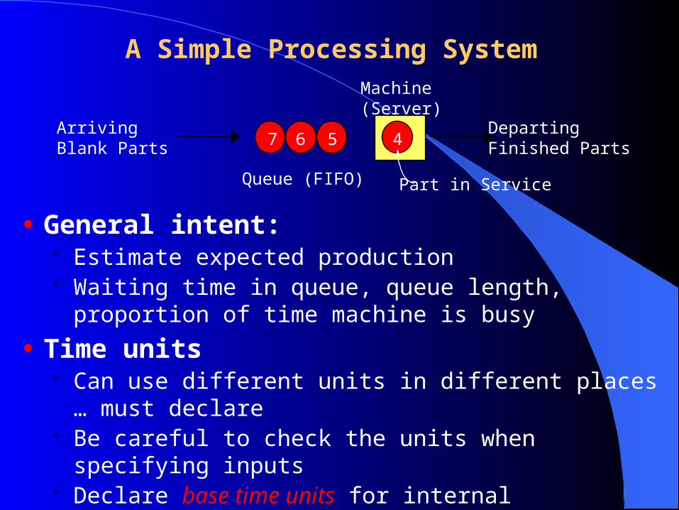
A Simple Processing System

ArrivingBlank Parts

DepartingFinished Parts

Machine(Server)

Queue (FIFO) Part in Service

4567

• General intent: Estimate expected production Waiting time in queue, queue length, proportion of time

machine is busy

• Time units Can use different units in different places … must declare Be careful to check the units when specifying inputs Declare base time units for internal calculations, outputs Be reasonable (interpretation, roundoff error)

Model Specifics

Initially (time 0) empty and idle Base time units: minutes Input data (assume given for now …), in minutes:

Part NumberArrival Time Interarrival Time Service Time1 0.00 1.73 2.902 1.73 1.35 1.763 3.08 0.71 3.394 3.79 0.62 4.525 4.41 14.28 4.466 18.69 0.70 4.367 19.39 15.52 2.078 34.91 3.15 3.369 38.06 1.76 2.3710 39.82 1.00 5.3811 40.82 . .. . . .. . . .

Stop when 20 minutes of (simulated) time have passed

N

WQN

ii

1

Output Performance Measures

Total production of parts over the run (P) Average waiting time of parts in queue:

Maximum waiting time of parts in queue:

N = no. of parts completing queue waitWQi = waiting time in queue of ith partKnow: WQ1 = 0 (why?)

N > 1 (why?)

iNi

WQmax,...,1

20

)(200 dttQ

Output Performance Measures

Time-average number of parts in queue:

Maximum number of parts in queue: Average and maximum total time in system of parts

(a.k.a. cycle time):

Q(t) = number of parts in queue at time t

)(max200

tQt

iPi

P

ii

TSP

TS

max,...,1

1 ,

TSi = time in system of part i

Output Performance MeasuresOutput Performance Measures

Utilization of the machine (proportion of time busy)

Many others possible (information overload?)

t

ttB

dttB

timeat idle is machine the if0

timeat busy is machine the if1)(,

20

)(200

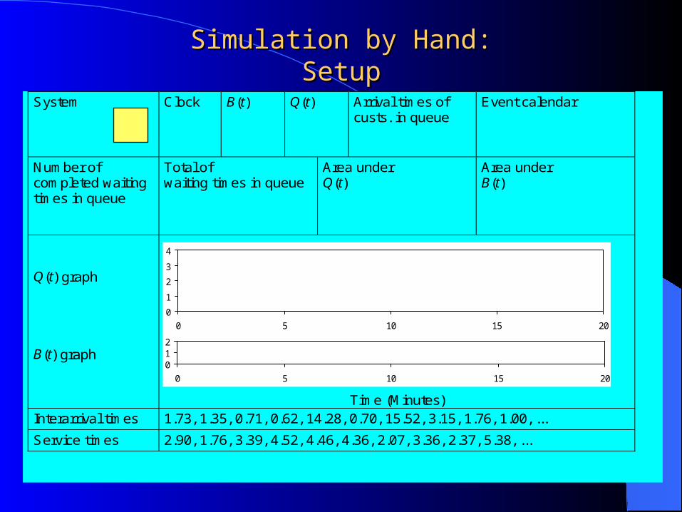
System

Clock

B(t)

Q(t)

Arrival times of custs. in queue

Event calendar

Number of completed waiting times in queue

Total of waiting times in queue

Area under Q(t)

Area under B(t)

Q(t) graph B(t) graph

Time (Minutes) Interarrival times 1.73, 1.35, 0.71, 0.62, 14.28, 0.70, 15.52, 3.15, 1.76, 1.00, ...

Service times 2.90, 1.76, 3.39, 4.52, 4.46, 4.36, 2.07, 3.36, 2.37, 5.38, ...

Simulation by Hand:Simulation by Hand:SetupSetup

0

1

2

3

4

0 5 10 15 20

012

0 5 10 15 20

System

Clock 0.00

B(t) 0

Q(t) 0


<empty>

Event calendar [1, 0.00, Arr] [–, 20.00, End]

Number of completed waiting times in queue 0

Total of waiting times in queue 0.00

Area under Q(t) 0.00

Area under B(t) 0.00



Service times 2.90, 1.76, 3.39, 4.52, 4.46, 4.36, 2.07, 3.36, 2.37, 5.38, ...

Simulation by Hand:Simulation by Hand:tt = 0.00, Initialize = 0.00, Initialize

0

1

2

3

4

0 5 10 15 20

012

0 5 10 15 20

System

Clock 0.00

B(t) 1

Q(t) 0


<empty>

Event calendar [2, 1.73, Arr] [1, 2.90, Dep] [–, 20.00, End]







Service times 2.90, 1.76, 3.39, 4.52, 4.46, 4.36, 2.07, 3.36, 2.37, 5.38, ...

Simulation by Hand:Simulation by Hand: tt = 0.00, Arrival of Part 1 = 0.00, Arrival of Part 1

0

1

2

3

4

0 5 10 15 20

012

0 5 10 15 20

1

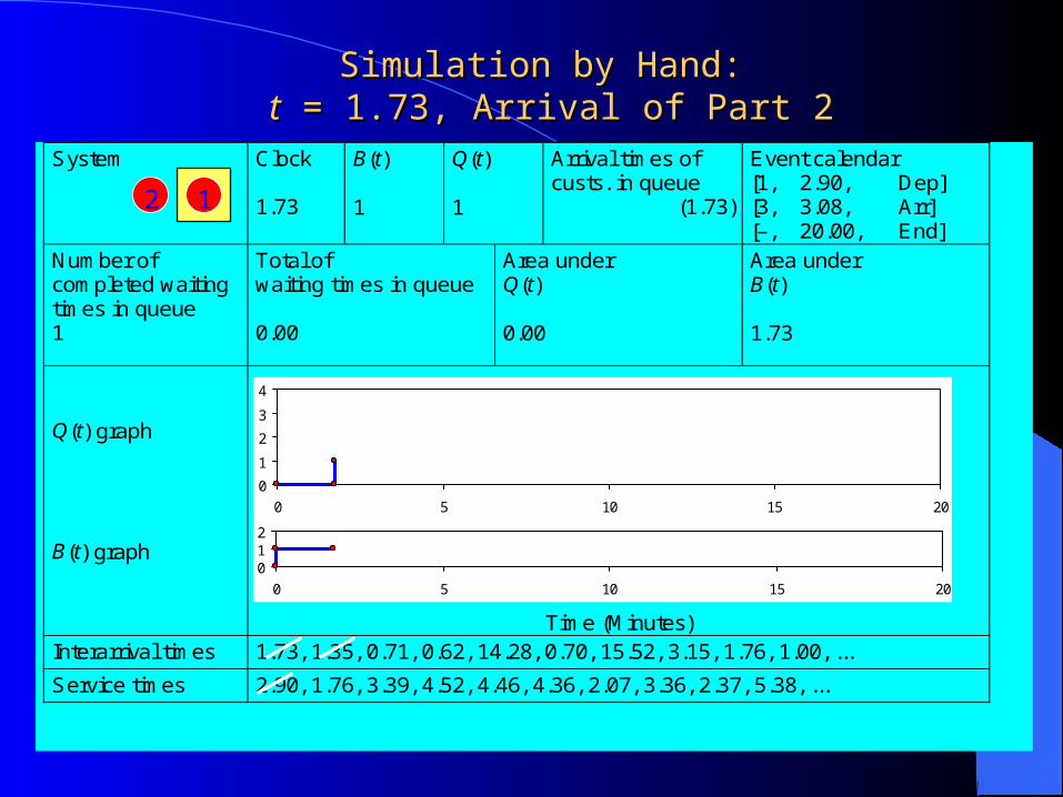
System

Clock 1.73

B(t) 1

Q(t) 1


(1.73)

Event calendar [1, 2.90, Dep] [3, 3.08, Arr] [–, 20.00, End]







Service times 2.90, 1.76, 3.39, 4.52, 4.46, 4.36, 2.07, 3.36, 2.37, 5.38, ...


0

1

2

3

4

0 5 10 15 20

012

0 5 10 15 20

12

System

Clock 2.90

B(t) 1

Q(t) 0


<empty>








Service times 2.90, 1.76, 3.39, 4.52, 4.46, 4.36, 2.07, 3.36, 2.37, 5.38, ...

Simulation by Hand:Simulation by Hand: tt = 2.90, Departure of Part 1 = 2.90, Departure of Part 1

0

1

2

3

4

0 5 10 15 20

012

0 5 10 15 20

2

System

Clock 3.08

B(t) 1

Q(t) 1


(3.08)








Service times 2.90, 1.76, 3.39, 4.52, 4.46, 4.36, 2.07, 3.36, 2.37, 5.38, ...


0

1

2

3

4

0 5 10 15 20

012

0 5 10 15 20

23

System

Clock 3.79

B(t) 1

Q(t) 2


(3.79, 3.08)








Service times 2.90, 1.76, 3.39, 4.52, 4.46, 4.36, 2.07, 3.36, 2.37, 5.38, ...


0

1

2

3

4

0 5 10 15 20

012

0 5 10 15 20

234

System

Clock 4.41

B(t) 1

Q(t) 3


(4.41, 3.79, 3.08)







Time (Minutes)

Interarrival times 1.73, 1.35, 0.71, 0.62, 14.28, 0.70, 15.52, 3.15, 1.76, 1.00, ...

Service times 2.90, 1.76, 3.39, 4.52, 4.46, 4.36, 2.07, 3.36, 2.37, 5.38, ...


0

1

2

3

4

0 5 10 15 20

012

0 5 10 15 20

2345

System

Clock 4.66

B(t) 1

Q(t) 2


(4.41, 3.79)







Time (Minutes)


Service times 2.90, 1.76, 3.39, 4.52, 4.46, 4.36, 2.07, 3.36, 2.37, 5.38, ...


0

1

2

3

4

0 5 10 15 20

012

0 5 10 15 20

345

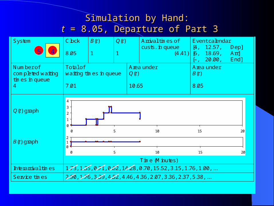
System

Clock 8.05

B(t) 1

Q(t) 1


(4.41)







Time (Minutes)


Service times 2.90, 1.76, 3.39, 4.52, 4.46, 4.36, 2.07, 3.36, 2.37, 5.38, ...


0

1

2

3

4

0 5 10 15 20

012

0 5 10 15 20

45

System

Clock 12.57

B(t) 1

Q(t) 0


()







Time (Minutes)


Service times 2.90, 1.76, 3.39, 4.52, 4.46, 4.36, 2.07, 3.36, 2.37, 5.38, ...


0

1

2

3

4

0 5 10 15 20

012

0 5 10 15 20

5

System

Clock 17.03

B(t) 0

Q(t) 0

Arrival times of custs. in queue ()

Event calendar [6, 18.69, Arr] [–, 20.00, End]






Time (Minutes)


Service times 2.90, 1.76, 3.39, 4.52, 4.46, 4.36, 2.07, 3.36, 2.37, 5.38, ...


0

1

2

3

4

0 5 10 15 20

012

0 5 10 15 20

System

Clock 18.69

B(t) 1

Q(t) 0

Arrival times of custs. in queue ()

Event calendar [7, 19.39, Arr] [–, 20.00, End] [6, 23.05, Dep]






Time (Minutes)


Service times 2.90, 1.76, 3.39, 4.52, 4.46, 4.36, 2.07, 3.36, 2.37, 5.38, ...


0

1

2

3

4

0 5 10 15 20

012

0 5 10 15 20

6

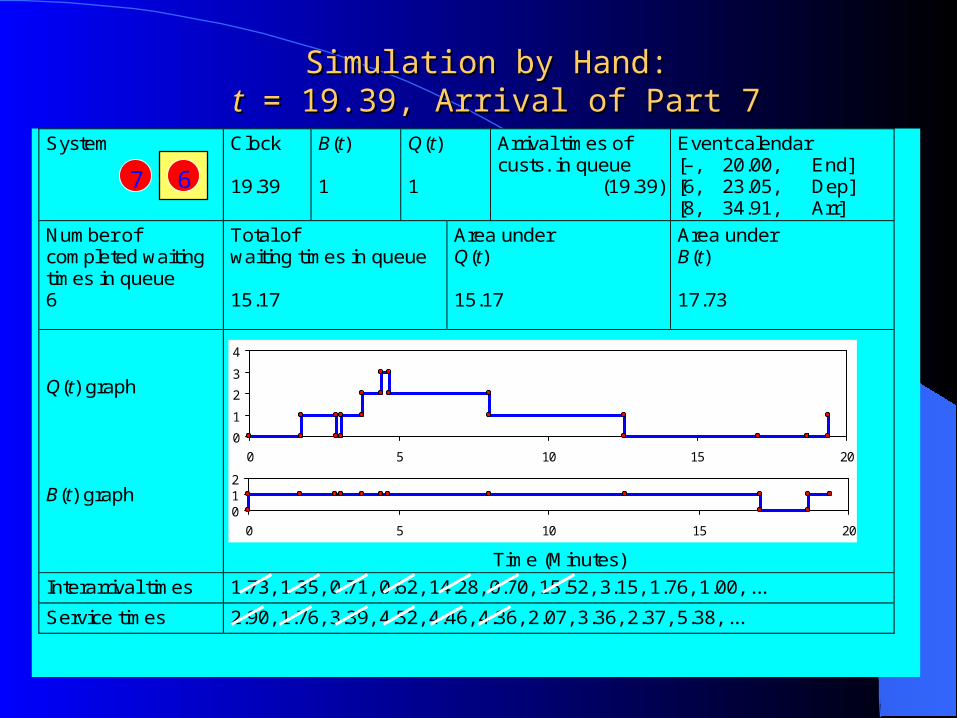
System

Clock 19.39

B(t) 1

Q(t) 1


(19.39)

Event calendar [–, 20.00, End] [6, 23.05, Dep] [8, 34.91, Arr]






Time (Minutes)


Service times 2.90, 1.76, 3.39, 4.52, 4.46, 4.36, 2.07, 3.36, 2.37, 5.38, ...


0

1

2

3

4

0 5 10 15 20

012

0 5 10 15 20

67

System

Clock 20.00

B(t) 1

Q(t) 1


(19.39)

Event calendar [6, 23.05, Dep] [8, 34.91, Arr]






Time (Minutes)


Service times 2.90, 1.76, 3.39, 4.52, 4.46, 4.36, 2.07, 3.36, 2.37, 5.38, ...

Simulation by Hand:Simulation by Hand: tt = 20.00, The End = 20.00, The End

0

1

2

3

4

0 5 10 15 20

012

0 5 10 15 20

67

Simulation by Hand:Simulation by Hand:Finishing UpFinishing Up

Average waiting time in queue:

Time-average number in queue:

Utilization of drill press:

part per minutes 53261715

queue in times of No.queue in times of Total

..

part 79020

7815value clock Final

curve under Area.

.)( tQ

less)(dimension 92020

3418value clock Final

curve under Area.

.)( tB

Comparing AlternativesComparing Alternatives

Usually, simulation is used for more than just a single model “configuration”

Often want to compare alternatives, select or search for the best (via some criterion)

Simple processing system: What would happen if the arrival rate were to double?– Cut interarrival times in half

– Rerun the model for double-time arrivals

– Make five replications

Results: Original vs. Double-Time ArrivalsResults: Original vs. Double-Time Arrivals

Original – circles Double-time – triangles Replication 1 – filled in Replications 2-5 – hollow Note variability Danger of making decisions

based on one (first) replication Hard to see if there are really

differences Need: Statistical analysis of

simulation output data

SIMAN SIMULATION LANGUAGE

– The Model Frame: Describes the logical flow of events within the system. The program should have the extension MOD (i.e., filename.MOD). Statements in the MODEL file are called BLOCKS.

– The Experiment Frame: Specifies the experimental conditions for executing the model. The program should have the extension EXP (i.e., filename.EXP). Statements in the EXPERIMENT file are called ELEMENTS.

A complete SIMAN model consists of a MODEL frame and an EXPERIMENT frame.

SIMAN RUNTIME PROCEDURESIMAN RUNTIME PROCEDURE

TEXTNAME.MOD

TEXTNAME.EXP

NAME.M NAME.E

NAME.P

NAME.OUT

MODEL EXPMT

LINKER

SIMAN

BASIC SIMAN MODELING

– ENTITIES: Items that flow through a system, such as customers, parts, trucks, etc.

– QUEUES: Waiting areas where the movement of entities is temporarily suspended.

– RESOURCES: System components that may be allocated to entities, such as machines, workers, bank tellers, etc.

– ATTRIBUTES: Represent values associated with individual entities, such as job type, arrival times, etc.

– GLOBAL VARIABLES: Represent values that describe the state of the system, such as number of job in the system, number of machines available, shift number, etc.

Example 1: The single Machine ProblemExample 1: The single Machine Problem

A single-Machine job shop processes two distinct products (or part types). Type 1 parts arrive every 10 minutes and require 4 minutes to process on the machine. Type 2 parts begin to arrive at time 5 and continue arriving every 6 minutes thereafter. Each type 2 part requires 3 minutes to process.

Determine the number of parts of each type that are processed in one 8-hour shift.

MachineBuffer

OutType 1 arrivals

Type 2 arrivals

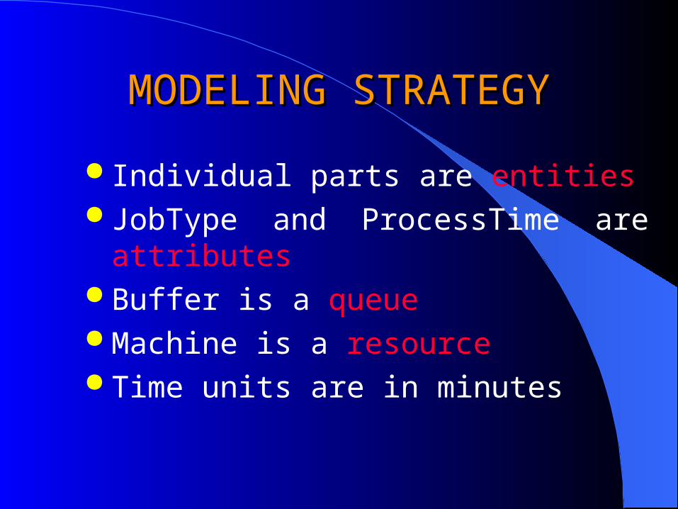
MODELING STRATEGYMODELING STRATEGY

Individual parts are entities JobType and ProcessTime are attributes Buffer is a queue Machine is a resource Time units are in minutes

FLOW LOGICFLOW LOGIC

– CREATE arriving jobs– ASSIGN values to ProcessTime and JobType– QUEUE the jobs for the machine in the Buffer– SEIZE the machine– DELAY by ProcessTime– RELEASE the machine– COUNT the JobType completed– DISPOSE of the finished jobs

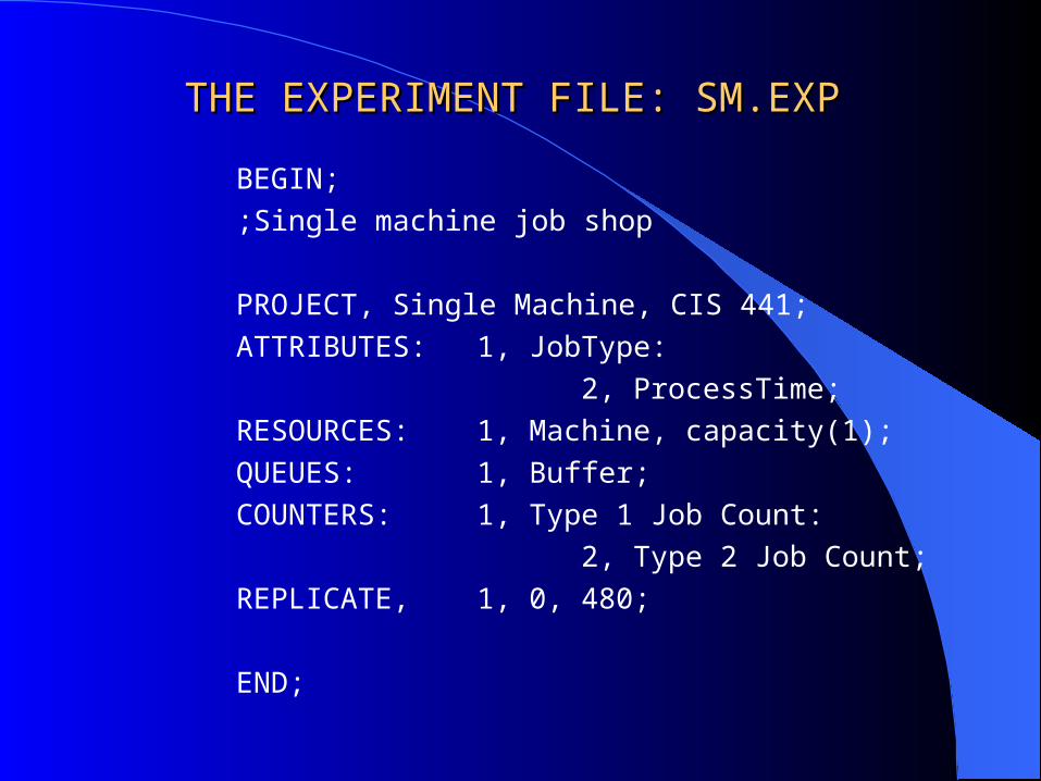
THE EXPERIMENT FILE: SM.EXPTHE EXPERIMENT FILE: SM.EXP

BEGIN;

;Single machine job shop

PROJECT, Single Machine, CIS 441;

ATTRIBUTES: 1, JobType:

2, ProcessTime;

RESOURCES: 1, Machine, capacity(1);

QUEUES: 1, Buffer;

COUNTERS: 1, Type 1 Job Count:

2, Type 2 Job Count;

REPLICATE, 1, 0, 480;

END;

THE MODEL FILE: SM.MOD

BEGIN;;Single machine job shop;Attributes: JobType, ProcessTime;Resource: Machine;Queue: Buffer

CREATE: 10; Create type 1 jobsASSIGN: JobType=1: ProcessTime=4:

NEXT(process);

CREATE, 1, 5: 6; Create type 2 jobsASSIGN: JobType=2:

ProcessTime=3;

process QUEUE, Buffer;SEIZE, 1: machine, 1;DELAY: ProcessTime;RELEASE: machine;

COUNT: JobType;DISPOSE;

END;

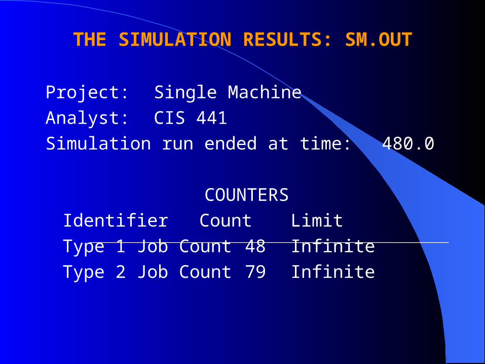
THE SIMULATION RESULTS: SM.OUT

Project: Single Machine

Analyst: CIS 441

Simulation run ended at time: 480.0

COUNTERS

Identifier Count Limit

Type 1 Job Count 48Infinite

Type 2 Job Count 79Infinite

Example 2: Modified SM ProblemExample 2: Modified SM Problem

Modify the single machine model such that the time between arrivals is exponentially distributed with means of 10 minutes and 6 minutes for job types 1 and 2 respectively. The processing times are uniformly distributed between 2 and 6 minutes for part type 1 and between 1.5 and 4.5 minutes for part type 2.

Collect statistics on the machine utilization, number of jobs waiting, job flowtime, and time between exits.

THE EXPERIMENT FILE: SM2.EXP

BEGIN;;Modified single machine job shop

PROJECT, Single Machine, CIS 441;

ATTRIBUTES: JobType: ProcessTime: ArrTime;RESOURCES: Machine;QUEUES: Buffer;COUNTERS: Type 1 Job Count:

Type 2 Job Count;

TALLIES: Flowtime:ExitPeriod;

DSTATS: NQ(Buffer), Queue Length:NR(Machine), Machine Utilization;

REPLICATE, 1, 0, 480;

END;

THE MODEL FILE: SM2.MOD

BEGIN;;Modified single machine job shop

CREATE: EXPO(10): MARK(ArrTime);ASSIGN: JobType=1: ProcessTime=UNIF(2,6):

NEXT(process);CREATE, 1, 5: EXPO(6):

MARK(ArrTime); ASSIGN: JobType=2:

ProcessTime=UNIF(1.5, 4.5);process QUEUE, Buffer;

SIEZE: machine;DELAY: ProcessTime;RELEASE: machine;

TALLY: 1, INTERVAL(ArrTime);TALLY: 2, BETWEEN;

COUNT: JobType;DISPOSE;

END;

THE SIMULATION RESULTS: SM2.OUT

Project: Single MachineAnalyst: CIS 441Simulation run ended at time: 480.0

TALLY VARIABLES

Identifier Average Variation Minimum Maximum ObservationsFlowtime 7.6548 .56697 1.5940 18.866 116ExitPeriod 4.1138 .61447 1.5089 18.022 115

DISCRETE CHANGE VARIABLES

Identifier Average Variation Minimum Maximum Final ValueQueue Length 1.0583 1.1847 .00000 5.0000 1.0000

Machine Utilization .80701 .48902 .00000 1.0000 1.0000

COUNTERS

Identifier Count LimitType 1 Job Count 43 InfiniteType 2 Job Count 73 Infinite

HW #1

1. Reading Chapters 1 and 2

2. 2-4

3. 2-5

4. Consider a manufacturing system comprising two different machines and a single operator who is shared between the two machines. Parts arrive with an exponentially distributed interarrival time with a mean of 3 minutes. The arriving parts are one of two types. Sixty percent of the arriving parts are type 1and are processed on machine 1. These parts require the operator for a one-minute setup operation. The remaining 40 percent are part type 2 and are processed on machine 2. These parts require the operator for a 1.5-minute setup operation. The service times (excluding the setup time) are normally distributed with a mean of 4.5 minutes and a standard deviation of 1 minute for type 1 parts and a mean of 7.5 minutes and a standard deviation of 1.5 minutes for type 2 parts.

Two different priority schemes have been proposed for allocating the operator between the two types of waiting jobs. The first scheme is to assign priority to the type 1 jobs. Under this proposal, a job type 2 setup will only be performed if there is no type 1 setups waiting to be performed. The second proposed scheme is to alternate the priority between the two job types.

Simulate each of these systems, using SIMAN language, for a 80-hour period; and collect statistics on the machine and operator utilization, the average number of parts waiting for each machine, and the average flow time for all parts.

Documents

SIMULATION TECHNIQUES. Introduction What is digital simulation? – Design a model for a real or proposed system – Execute the model on a computer – Analyze