Simulation Technique of Velocity-Based Discrete-time ... · discrete-time control system for an open architectural industrial robot, it is required from the points of view concerning

The Open Automation and Control Systems Journal, 2008, 1, 31-43 31123

Open Access

Simulation Technique of Velocity-Based Discrete-time Control System

with Intelligent Control Concepts for Open Architectural Industrial

Robots

Fusaomi Nagata∗

Department of Electronics and Computer Science, Tokyo University of Science, Yamaguchi

Abstract: Industrial robots have drastically rationalized many kinds of manufacturing processes in

industrial fields. For this decade, open architectural industrial robots have been produced from several

industrial robot makers such as KAWASAKI Heavy Industries, Ltd., MITSUBISHI Heavy Industries, Ltd.

and YASKAWA Electric Corp. and so on. Open architecture described in this article means that the

servo system and kinematics of the robot are technically opened, so that various applications required in

industrial fields are allowed to be planned and developed at the user side. For example, non-taught oper-

ation by using a CAD/CAM system can be considered due to the opened accurate kinematics. Also, force

control strategy using a force sensor can be implemented due to the opened servo system. In this article, a

simulation technique of velocity-based discrete-time control system for open architectural industrial robots

is introduced by giving examples of intelligent control methods. In order to develop a novel velocity-based

discrete-time control system for an open architectural industrial robot, it is required from the points of

view concerning safety, cost and easiness to preliminarily examine and evaluate the characteristics and

performance. In such a case, the proposed simulation technique is useful.

INTRODUCTIONIndustrial robots have drastically rationalized many kinds

of manufacturing processes in industrial fields. The user in-

terface provided by the robot maker has been almost limited

to so-called the teaching pendant. The teaching pendant is

a useful and safe tool to obtain positions and orientations at

the tip of a robot along a desired trajectory, but the teaching

task is very complicated and time-consuming task. Espe-

cially, when the target trajectory is a free curved line, many

through points must be given to acquire a smooth trajectory;

the task is further not easy.

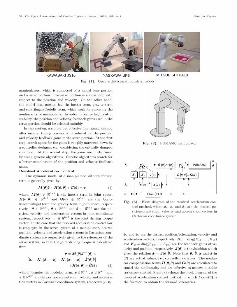
For this decade, open architectural industrial robots as

shown in Fig. (1) have been produced from several industrial

robot makers such as KAWASAKI Heavy Industries, Ltd.,

MITSUBISHI Heavy Industries, Ltd. and YASKAWA Elec-

tric Corp. and so on. Open architecture described in this

article means that the servo system and kinematics of the

robot are technically opened, so that various applications

required in industrial fields are allowed to be planned and

developed at the user side. For example, non-taught opera-

tion by using a CAD/CAM system can be considered due to

the opened accurate kinematics. Also, force control strategy

using a force sensor can be easily implemented due to the

technically opened discrete-time servo system.

It is now possible to model and simulate many types

of robots. For example, Chen et al. presented a new de-

sign of an environment for simulation, animation, and vi-

Address corresponding to this author at the Department of Electronics and

Computer Science, Tokyo University of Science, Yamaguchi;

E-mail: [email protected]

sualization of sensor-driven robots. Although conventional

computer-graphics-based robot simulation and animation

software packages lacked of capabilities for robot sensing sim-

ulation, the system was designed to overcome the deficiency

[1]. Also, Benimeli et al. addressed the implementation and

comparison of an indirect and a direct identification proce-

dures on an industrial robot provided with an open control

architecture. The estimation of dynamic parameters in me-

chanical systems constituted an issue of crucial importance

for dynamic simulation applications where high accuracy was

required [2].

In this article, we present a simulation technique of

velocity-based discrete-time control system for open archi-

tectural industrial robots by giving and combining examples

of intelligent control concepts such as genetic algorithms,

fuzzy control and neural network. In order to develop a

novel velocity-based control system represented in discrete-

time domain for an open architectural industrial robot, it is

required from the points of view concerning safety, cost and

easiness to preliminarily examine and evaluate the character-

istics and performance. In such a case, the proposed simu-

lation techniques will be useful. The validation and promise

are evaluated through simulations by using a dynamic model

of PUMA560 manipulator as shown in Fig. (2) [3], [4].

BASIC SERVO SYSTEMIn order to simulate an industrial robot, first of all, a servo

system is considered and designed. Here, the resolved accel-

eration controller [5] is picked up in a servo system. The

resolved acceleration control method or computed torque

control method is used for nonlinear control of industrial

1874-4443/08 2008 Bentham Open

32 The Open Automation and Control Systems Journal, 2008, Volume 1 Fusaomi Nagata

KAWASAKI JS10 YASKAWA UP6 MITSUBISHI PA10

Fig. (1). Open architectural industrial robots.

manipulators, which is composed of a model base portion

and a servo portion. The servo portion is a close loop with

respect to the position and velocity. On the other hand,

the model base portion has the inertia term, gravity term

and centrifugal/Coriolis term, which work for canceling the

nonlinearity of manipulator. In order to realize high control

stability, the position and velocity feedback gains used in the

servo portion should be selected suitably.

In this section, a simple but effective fine tuning method

after manual tuning process is introduced for the position

and velocity feedback gains in the servo portion. At the first

step, search space for the gains is roughly narrowed down by

a controller designer, e.g. considering the critically damped

condition. At the second step, the gains are finely tuned

by using genetic algorithms. Genetic algorithms search for

a better combination of the position and velocity feedback

gains.

Resolved Acceleration Control

The dynamic model of a manipulator without friction

term is generally given by

M(„)„ + H(„, „) + G(„) = fi (1)

where, M(„) ∈ ℜ6×6 is the inertia term in joint space.

H(„, „) ∈ ℜ6×1 and G(„) ∈ ℜ6×1 are the Corio-

lis/centrifugal term and gravity term in joint space, respec-

tively. „ ∈ ℜ6×1, „ ∈ ℜ6×1 and „ ∈ ℜ6×1 are the po-

sition, velocity and acceleration vectors in joint coordinate

system, respectively. fi ∈ ℜ6×1 is the joint driving torque

vector. In the case that the resolved acceleration control law

is employed in the servo system of a manipulator, desired

position, velocity and acceleration vectors in Cartesian coor-

dinate system are respectively given to the references of the

servo system, so that the joint driving torque is calculated

from

fi = M(„)J−1(„) ×[xr + Kv{xr − x} + Kp{xr − x} − J(„)„

]+H(„, „) + G(„) (2)

where,ˆdenotes the modeled term. x ∈ ℜ6×1, x ∈ ℜ6×1 and

x ∈ ℜ6×1 are the position/orientation, velocity and accelera-

tion vectors in Cartesian coordinate system, respectively. xr,

Fig. (2). PUMA560 manipulator.

PUMA560

( )θJ

θθ&( ) ( )θJθM 1ˆ −

( ) ( )θGθθH ˆ,ˆ +&

( )θFkine

( )θJ&

τ

+ +

+

+ −

−

−++

+

pK

rxx

x&rx&

rx&&

vK

Fig. (3). Block diagram of the resolved acceleration con-

trol method, where xr, xr and xr are the desired po-

sition/orientation, velocity and acceleration vectors in

Cartesian coordinate system.

xr and xr are the desired position/orientation, velocity and

acceleration vectors, respectively. Kv = diag(Kv1, . . . , Kv6)

and Kp = diag(Kp1, . . . , Kp6) are the feedback gains of ve-

locity and position, respectively. J(„) is the Jacobian which

gives the relation x = J(„)„. Note that „, „, x and x in

(2) are actual values, i.e., controlled variables. The nonlin-

ear compensation terms H(„, „) and G(„) are calculated to

cancel the nonlinearity and are effective to achieve a stable

trajectory control. Figure (3) shows the block diagram of the

resolved acceleration control method, in which Fkine(„) is

the function to obtain the forward kinematics.

Simulation Technique of Velocity-Based The Open Automation and Control Systems Journal, 2008, Volume 1 33

Fine Gain Tuning Considering the Critically Damped

Condition

A basic gain tuning method considering the critically

damped condition is explained giving an example. If it is

assumed that the modeled termsˆare exact, then the nonlin-

earity of the robot dynamics can be canceled. Substituting

(2) into (1) gives the following second order error system.

e + Kve + Kpe = 0 (3)

where, e = xr − x. Accordingly, Kv and Kp are selected

suitably, e.g., considering the critically dumped condition

given by

Kvi = 2√

Kpi (i = 1, . . . , 6) (4)

so that desirable responses can be obtained if under the ideal

condition as given by (3). It should be noted, however, that

there exists nonlinearity such as Coulomb friction and vis-

cous friction. The robotic dynamic model with the friction

term is written by

M(„)„ + H(„, „) + G(„) + F r(„, „) = fi (5)

where, F r(„, „) ∈ ℜ6×1 is the friction term composed of

viscous friction and Coulomb friction. Also, because M(„),

H(„, „) and G(„) in (2) implicitly include undesirable mod-

eled treatment error, the velocity and position gains in the

servo portion should be more finely tuned after basic gain

tuning. In the reminder of this section, genetic algorithms

are applied to search for more suitable gains.

Desired Trajectory

For instance, in order to apply the resolved acceleration

control method to the manipulator, the desired trajectory

composed of xr, xr and xr in Cartesian coordinate system

must be prepared. First of all, the desired trajectory in

Cartesian coordinate system is designed as shown in Fig.

(4), in which the manipulator moves from the initial pose to

the final pose. In this case, the robot stretches the arm tip

500 mm to the x-direction. The manipulator is still in initial

and final poses. The desired trajectory xr, xr and xr are cal-

culated through a 4-1-4 order polynomial equation. We can

design various trajectories with combination of acceleration

time, constant velocity time and deceleration time. Desired

angle „r, angle velocity „r and acceleration „r in joint space

are transformed from xr, xr and xr by respectively using the

inverse kinematics, Jacobian J(θ) and sampling width ∆t.

An example that consists of desired joint angle, angle

velocity and acceleration is shown in Fig. (5), which are

transformed from the xr, xr and xr in Fig. (4). The tra-

jectory in joint space makes the robot follow the motion as

shown in Fig. (4). To obtain satisfactory and safe control

performance without falling a singularity, Kv and Kp are

roughly tuned in advance with trial and error, considering

the combination around critically damped condition. We call

Initial pose Final pose

Fig. (4). Trajectory following control problem.

0 1 2 3

Joint

veloc

ity ra

d/s

-0.5

-1

0

0.5

Desir

ed an

gle ra

d

Time s

J1, J4, J6

J2J5

J3

J1, J4, J6

J2J5

J3

-0.5-1

00.5

1

-1.5

Joint

acce

lerati

on ra

d/s2

J3

J2J5 J1, J4, J6

-0.5-1

00.5

1.51

2

Fig. (5). Desired joint angle „r, velocity „r and accelera-

tion „r in joint space.

this the initial manual tuning process. Two search spaces for

Kv and Kp are obtained after the manual tuning process,

so that Kv and Kp must be further tuned finely within the

searched spaces to achieve a desirable motion without large

overshoots and oscillations. In the next subsection, we pro-

pose a systematic tuning method using genetic algorithms

which can be applied to after the manual tuning process.

Fine Gain Tuning by Using Genetic Algorithms

The gain tuning after designing a robotic servo controller

is an important and indispensable task to realize a smooth

motion control system. The proposed gain tuning process

consists of two steps. The first step is conducted to nar-

row down the search space for gains by operator’s manual

gain tuning while considering the circumference of the crit-

ically damped conditions given by (4). The ranges for gain


1vK 5vK2vK 3vK 4vK 6vK 1pK 5pK2pK 3pK 4pK 6pK

Fig. (6). Genotype of Kv and Kp which means an indi-

vidual.

search are narrowed down between the minimum Kvi, Kpi

and maximum Kvi, Kpi. The objective of the second step is

to finely search for a more superior combination of Kvi and

Kpi within the search space by using genetic algorithms [6],

[7].

The genetic algorithm is used to optimize Kvi and

Kpi(i = 1, . . . , 6) which are the diagonal elements of Kv

and Kp. In order to apply genetic algorithms, Kvi and

Kpi are transformed into a genotype. Diagonal elements

Kvi and Kpi are encoded into 8 bits binary code and an

individual is composed of 96(= 8 × 12) bits. A population

has 60 individuals. Each individual in initial population is

generated within expectable range considered in the initial

manual tuning process. For example, we have preliminar-

ily confirmed by randomly conducted manual tuning that if

each element of Kv and Kp in (2) is set to 50 ≤ Kvi ≤ 200

and 10 ≤ Kpi ≤ 50000 (i = 1, . . . , 6) then an undesirable

singularity does not tend to occur. The singularity is a rep-

resentative result after the system becomes unstable.

The elite survivable strategy is adopted in the selection

process, where superior six individuals can survive to next

generation as elites. Crossover and mutation which are the

representative GA operations are not applied to the geno-

types of the elites. Other remained 54 individuals are yielded

by tournament selection. The genotype including the Kv

and Kp is shown in Fig. (6). Each individual is evaluated

by applying (2) to the trajectory following control problem

shown in Fig. (4). The evaluation value Ev is calculated

based on the square root of the sum of each directional error

squared every sampling time, which is obtained by

Ev =

T∆t∑

k=1

√√√√ 3∑i=1

{ei(k)}2 (6)

where the error ei(k) (i = 1, 2, 3) is the x-, y- and z-

directional position errors in Cartesian space. T and ∆t are

the simulation time needed for a trajectory following control

and sampling period, respectively. This is a minimization

problem, where individuals with smaller fitness Ev can sur-

vive as elites to the next generation.

Tuning Result

Simulations were carried out by using the dynamic model

of PUMA560 manipulator on MATLAB system. The robotic

dynamics with the friction torque term given by (5) is ap-

plied. The friction torque term F r consists of the viscous

friction torque and Coulomb friction torque, which is repre-

sented by

F r(„, „) = BG2r„ + Grfi c{sign(„)} (7)

Table 1. Parameters of GA operation in case of resolved

acceleration control law

Population size 60

Number of elites 6

Selection Tournament selection

Crossover Uniform crossover (rate=87.5%)

Mutation Random mutation (rate=4.17%)

Search space of Kvi 0.001 ≤ Kvi ≤ 220

Search space of Kpi 0.001 ≤ Kpi ≤ 40000

Maximum generation 100

where B is the coefficient matrix of viscous friction at each

motor, Gr is the reduction gear ratio matrix which repre-

sents the motor speed to joint speed, and fi c{sign(„)} is

the Coulomb friction torque appeared at each motor. If

sign(θi) > 0, then τci = τ+ci ; if sign(θi) < 0, then τci = τ−

ci .

In simulations, B and Gr are set to diag(0.0015, 0.0008,

0.0014, 0.0001, 0.0001, 0.0000) and diag(-62.6, 107.8, -53.7,

76.0, 71.9, 76.7), respectively; fi +c and fi−

c are set to [0.395

0.126 0.132 0.011 0.009 0.004]T and [-0.435 -0.071 -0.105 -

0.017 -0.015 -0.011]T , respectively [3].

Before applying the GA operation, we broadly inves-

tigated the characteristics of the trajectory following con-

trol, while changing the combination of Kv and Kp. As the

result, the ranges in which the robot could move without

falling a singularity were respectively 0.001 ≤ Kvi ≤ 220

and 0.001 ≤ Kpi ≤ 40000 (i = 1, . . . , 6), so that the search

space for GA was limited within these ranges. The uniform

crossover was employed to the individuals with a high proba-

bility rate 87.5% (7/8) and the reverse action with mutation

rate 4.17% (1/24) is given to all bits forming 54 individuals.

Other parameters for GA operations are tabulated in Table

1. As an example of the tuning effectiveness, the variation

of minimum fitness is shown in Fig. (7). It is observed that

more excellent individuals have been selected through the

alternation of generations with GA operations. After 100

generations, the phenotype of the best individual is repre-

sented by

Kv = diag(157, 204, 171, 181, 192, 76) (8)

Kp = diag(23137, 7412, 24471, 7922, 13725, 5882) (9)

When above gains were given, the minimum fitness Ev be-

came 0.5241 by (6).

Figure (8) shows the simulation results which are per-

formed by the gains with the minimum fitness. The upper

figure in Fig. (8) shows the controlled angle trajectories

of joints 2 and 3. The second figure similarly shows the

angle velocities. The third and lower figures respectively

illustrate the friction torques acting at the joints 2 and 3

which are given by (7). For example, it can be observed


20 40 60 80 1000.520.53

0.540.55

0.56

Generation No.

Best

fitn

ess

Ev

0

With considering friction torques

0.570.580.59

Fig. (7). Evolutionary history in case that the resolved

acceleration control law was employed.

from the second figure in Fig. (8) that sign(θ2) and sign(θ3)

are frequently changed around the start time and end time.

According to the changes of sign(θ2) and sign(θ3), the large

influence of Coulomb friction can be also observed around

the corresponding time area in the third and lower figures.

It is also observed that the best combination of Kvi and Kpi

among obtained through the GA operation almost has the

under damped condition given by

Kvi < 2√

Kpi (i = 1, . . . , 6) (10)

This suggests that under damped situation is suitable for

such a robotic trajectory following control with time-varying

references as shown in Fig. (5).

In this section, we have preliminarily described the re-

solved acceleration controller as an example of robotic servo

system which is surely incorporated in open architectural in-

dustrial robots. A simple but effective finely tuning method

using genetic algorithms has been also introduced as one

of intelligent control methodologies. Such a servo system

is technically opened when an open architectural industrial

robot is provided, so that we have only to make the desired

trajectory xr, xr and xr according to each task. Therefore,

when a force control method is implemented, we have only

to design the system so that the manipulated variables of

the force control method are represented by xr, xr and xr

in discrete-time domain.

DYNAMIC SIMULATIONWhen a computer is used to control an industrial robot, the

control law is generally represented by a discrete-time control

system. In this section, it is described on how to simulate

and evaluate the velocity-based discrete-time control system

which is implemented into an open architectural industrial

robot. Let’s consider the impedance model following force

control as an example of velocity-based discrete-time control

systems. In order to conduct a simulation with a robotic

dynamic model, manipulated variables written by velocity

commands in discrete-time domain must be transformed into

0 1 2 3

Joint

veloc

ity ra

d/s

-1

0

0.8

Contr

olled

angle

rad

Time s

J2

J3

J2

J3

-0.5

-1

0

0.5

1

-1.5

J3

-10

J2

0

10

20

Fricti

on to

rque a

t J2

NmFri

ction

torqu

e at J

3 Nm

0

-8-6-4-2

246

J2

J3

Fig. (8). Simulation result in case of using the gains with

minimum fitness.

joint driving torques.

Impedance Model Following Force Control

Impedance control is one of the effective control strategies

for a manipulator to desirably reduce or absorb the external

force from an environment [8]. It is characterized by an abil-

ity which controls the mechanical impedance such as mass,

damping and stiffness acting at joints. Impedance control

does not have a force control mode or a position control

mode but it is a combination of force and velocity. In or-

der to control the contact force acting between the arm tip

and environment, we have proposed the impedance model

following force control methods (IMFFC) that can be easily

implemented in industrial robots with an open architecture

controller [9]. The desired impedance equation in Cartesian

space for a robot manipulator is designed by

Md(x − xd) + Bd(x − xd) + SKd(x − xd)

= SF + (I − S)Kf (F − F d) (11)

where x ∈ ℜ3, x ∈ ℜ3 and x ∈ ℜ3 are the position, ve-

locity and acceleration vectors, respectively. Md ∈ ℜ3×3,


Bd ∈ ℜ3×3 and Kd ∈ ℜ3×3 are the coefficient matrices of

desired mass, damping and stiffness, respectively. F ∈ ℜ3

is the force vector. Kf ∈ ℜ3×3 if the force feedback gain

matrix. xd, xd, xd and F d are the desired position, velocity,

acceleration and force vectors, respectively. S is the switch

matrix to select force control mode or compliance control

mode. If S = 0, (11) becomes force control mode in all di-

rections; whereas if S = I it becomes compliance control

mode in all directions. Here, I is the identity matrix. Md,

Bd, Kd and Kf are set to positive-definite diagonal matri-

ces.

When force control mode is selected in all directions, i.e.,

S = 0, defining X = x − xd gives

X = −M−1d BdX + M−1

d Kf (F − F d) (12)

Here, the stability of (12) is briefly considered at the equi-

librium by using Lyapunov stability analysis. The candidate

of Lyapunov function [10] is proposed by

V (X) =1

2XT X (13)

which is continuous and everywhere nonnegative. Differen-

tiating (13) gives

V (X) = XT X = XT (−M−1d BdX)

= −XT M−1d BdX (14)

which is everywhere non-positive since M−1d Bd is a positive

definite diagonal matrix. Therefore, (13) is indeed a Lya-

punov function for the system given by (12). V (X) can be

zero only at X = 0, everywhere else V (X) decreases, so that

(12) is asymptotically stable.

In general, (12) can be resolved as

X = e−M−1d

BdtX(0)

+

∫ t

0

e−M−1d

Bd(t−τ)M−1d Kf (F − F d)dτ (15)

In the following, we consider the form in the discrete time

k using a sampling time ∆t. If it is assumed that Md, Bd,

Kf , F and F d are constant at ∆t(k − 1) ≤ t < ∆tk, then

defining X(k) = X(t)|t=∆tk leads to the recursive equation

given by

X(k) = e−M−1d

Bd∆t X(k − 1)

−(e−M−1

dBd∆t − I

)B−1

d Kf{F (k) − F d} (16)

Remembering X = x− xd, giving xd = 0 in the direction of

force control, and adding an integral action, the equation of

velocity command in terms of Cartesian space is derived by

x(k) = e−M−1d

Bd∆t x(k − 1)

−(e−M−1

dBd∆t − I

)B−1

d Kf{F (k) − F d}

+Ki

k∑n=1

{F (n) − F d} (17)

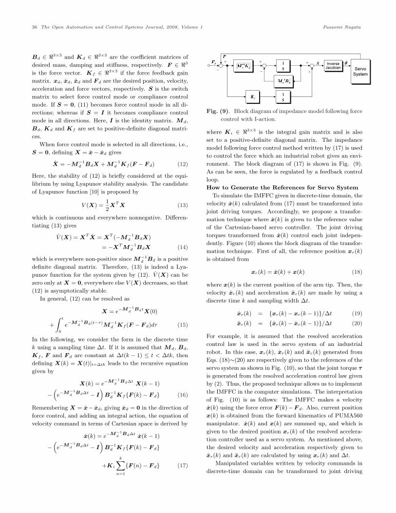
ServoSystemServoSystem

+_

+_

+

+

iK

x& InverseJacobianInverseJacobian

θ&

Fig. (9). Block diagram of impedance model following force

control with I-action.

where Ki ∈ ℜ3×3 is the integral gain matrix and is also

set to a positive-definite diagonal matrix. The impedance

model following force control method written by (17) is used

to control the force which an industrial robot gives an envi-

ronment. The block diagram of (17) is shown in Fig. (9).

As can be seen, the force is regulated by a feedback control

loop.

How to Generate the References for Servo System

To simulate the IMFFC given in discrete-time domain, the

velocity x(k) calculated from (17) must be transformed into

joint driving torques. Accordingly, we propose a transfor-

mation technique where x(k) is given to the reference value

of the Cartesian-based servo controller. The joint driving

torques transformed from x(k) control each joint indepen-

dently. Figure (10) shows the block diagram of the transfor-

mation technique. First of all, the reference position xr(k)

is obtained from

xr(k) = x(k) + x(k) (18)

where x(k) is the current position of the arm tip. Then, the

velocity xr(k) and acceleration xr(k) are made by using a

discrete time k and sampling width ∆t.

xr(k) = {xr(k) − xr(k − 1)}/∆t (19)

xr(k) = {xr(k) − xr(k − 1)}/∆t (20)

For example, it is assumed that the resolved acceleration

control law is used in the servo system of an industrial

robot. In this case, xr(k), xr(k) and xr(k) generated from

Eqs. (18)∼(20) are respectively given to the references of the

servo system as shown in Fig. (10), so that the joint torque fi

is generated from the resolved acceleration control law given

by (2). Thus, the proposed technique allows us to implement

the IMFFC in the computer simulations. The interpretation

of Fig. (10) is as follows: The IMFFC makes a velocity

x(k) using the force error F (k)−F d. Also, current position

x(k) is obtained from the forward kinematics of PUMA560

manipulator. x(k) and x(k) are summed up, and which is

given to the desired position xr(k) of the resolved accelera-

tion controller used as a servo system. As mentioned above,

the desired velocity and acceleration respectively given to

xr(k) and xr(k) are calculated by using xr(k) and ∆t.

Manipulated variables written by velocity commands in

discrete-time domain can be transformed to joint driving


IMFFC

PUMA560+

_

ResolvedAccelerationController

z1

t∆1

z1

t∆1

+( )kx&

( )kx

( )krx

( )krx&

( )krx&&

τ

( )kF

dF+

+

+_

_

: Current position

IMFFC : Impedance Model Following Force Controller

: Force sensor measurement

Fig. (10). Block diagram of impedance model following force controller, in which xr(k), xr(k) and xr(k) are transformed into

the joint driving torque fi .

torques due to the proposed scheme as shown in Fig. (10),

so that various velocity-based control methodologies writ-

ten in discrete-time domain developed for open architectural

industrial robots have been able to be easily simulated.

IN CASE OF FUZZY CONTROLFuzzy Force Control

To improve the force control performance in the envi-

ronment with unknown dynamics or curved surface, how

to construct the fuzzy controller by using the servo system

introduced in the previous section is first described. The

main feature of the fuzzy force controller is that it gener-

ates proper position compensations as feedforward command

so that overshoots and oscillations in the direction of force

control can be suppressed satisfactorily. A profiling control

simulation using the dynamics of PUMA560 manipulator is

shown to demonstrates the effectiveness under an environ-

ment with time-varying stiffness.

If a force controlled manipulator is applied to a pro-

filing task, the change of environmental stiffness or shape

causes undesirable force error. The fuzzy force controller

works to reduce the force error. The fuzzy controller gen-

erates velocity vector, i.e., position compensation vector

∆x(k) = [∆x(k) ∆y(k) ∆z(k)]T as a feedforward control ac-

cording to the force error and its rate every sampling time.

For example, let’s consider the x-directional compensation.

Fuzzy inputs are the force error and its rate defined as

ex(k) = Fdx − Fx(k) (21)

∆ex(k) ={ex(k) − ex(k − 1)}

∆t(22)

where Fdx and Fx(k) are the desired force and sensed force,

respectively. Following the fuzzy approach, if the informa-

tion on only x-direction is used, the fuzzy rules are described

by

Rule 1 IF ex(k) is A1 and ∆ex(k) is B1, THEN ∆x(k) = c1



...

Rule L IF ex(k) is AL and ∆ex(k) is BL, THEN ∆x(k) = cL

where Ai(i = 1, ..., L) and Bi are the i-th antecedent fuzzy

sets for two fuzzy inputs ex(k) and ∆ex(k); ci is the con-

sequent constant value at the i-th rule; L is the fuzzy rule

number. The confidence of the antecedent part at the i-th

rule is obtained by

ωi = µAi{ex(k)} ∧ µBi{∆ex(k)} (23)

where µX(•) denotes the confidence of a fuzzy set labeled by

X. Therefore, the fuzzy position compensation is calculated

by

∆x(k) =

∑L

i=1ωici∑L

j=1ωj

(24)

The position compensation of other directions, ∆y(k) or

∆z(k) is similarly calculated by the same procedure. Note

that, the fuzzy set used is the following Gaussian type mem-

bership function

µX(x) = exp{log(0.5)(x − α)2β2} (25)

where α is the center of membership function and β is the

reciprocal value of standard deviation. Figures (11) and

(12) show the designed antecedent membership functions for

ex(k) and ∆ex(k), respectively. Each reciprocal value of the

standard deviation are 66.7 and 100, respectively. The cor-

responding constant values in consequent part are tabulated

in Table 2. It is expected that the proposed fuzzy force con-

troller will improve the force control performance.

Simulation of Fuzzy Force Control

In this subsection, a profiling control as shown in Fig. (13)

is conducted and analyzed in detail. And the promise of the

proposed method shown in Fig. (15) is evaluated through the

profiling control simulation.There are two important factors

that prevent the stable profiling control. The one is that


-9 -6 -3 0 3 6 9 x 10 - 2

NB NM NS PS PM PB

0

0.5

1

Fig. (11). Antecedent membership functions for ex(k).

NB NM NS PS PM PB

0

0.5

1

-6 -4 -2 0 2 4 6 x 10 - 2

Fig. (12). Antecedent membership functions for ∆ex(k).

the dynamics of the object is almost unknown, and perhaps

changes frequently. The other is that how curved surface

the object has. In practice, robots for polishing and sanding

must deal with such objects. It is assumed that the object

with an inclined and flat plane is fixed in the robot workspace

as shown in Fig. (13). The end-effector contacts with the

object; it is tried to control the contact force from normal

direction of the slope to converge to a reference of 1 N. It is

also assumed that the contact force F (k) is generated by

F (k) = −Bmx(k) − Km{x(k) − xm} (26)

where Bm Ns/m and Km N/m are the viscosity and stiff-

ness coefficients of the object to be positive definite diag-

onal matrices, and xm is the initial contact position. In

the following simulation, the stiffness of the object Km =

diag(Kmx, Kmy, Kmz) varies as follows:

Kmx = 100000 + 30000 × sin(3kπ) (27)

Table 2. Constant values in consequent part [×10−4 mm]

PPPPPPPPex(k)

∆ex(k)NB NM NS PS PM PB

NB -16.0 -14.0 -12.0 -8.0 -6.0 -4.0

NM -9.6 -8.4 -7.2 -4.8 -3.6 -2.4

NS -3.2 -2.8 -2.4 -1.6 -1.2 -0.8

PS 0.8 1.2 1.6 2.4 2.8 3.2

PM 2.4 3.6 4.8 7.2 8.4 9.6

PB 4.0 6.0 8.0 12.0 4.0 16.0

Top of a robot armQ

6π

P

sz

Bm : ViscosityKm : Siffness

so -sx sy sz : Sensor coordinate system

sy

sxso

Fig. (13). Profiling control situation.

0 1 2 3 4Time s

7

8

9

10

11

12

Stiffn

ess o

f work

piece

x 104

N/m

13X-direction Z-direction

Fig. (14). Time histories of environmental stiffness in x-

and z-directions.

Kmz = 100000 + 30000 × sin(4kπ + π/2) (28)

which is illustrated as shown in Fig. (14). The viscosity is

fixed to Bm = diag(15, 15, 15) Ns/m. Here, we control the

z-directional contact force and y-directional trajectory (i.e.,

from point P to Q shown in Fig. (13)) in sensor coordinate

system. Also, we set up the manipulator as PUMA560 [3],

its dynamics is given by

Mx(„)x + Hx(„, „) + Gx(„) = J−T („)fi + F (29)

where Hx(„) is the Coriolis and centrifugal forces, Gx(„)

is the gravity term, J(„) is the Jacobian matrix, and fi is

the joint driving torque. Note that the subscript x means

the value in Cartesian space. The dynamics is solved by the

Runge-Kutta method on Matlab system. In this case, the

resolved acceleration controller is used in the servo system

shown in Fig. (15), and the xr(k) is generated by

xr(k) = x(k) + ∆x(k) + x(k) (30)


IMFFCPUMA560

+

+

_

ResolvedAcceleration

Controller

Fuzzy Force Controller

z1

t∆1

z1

t∆1

+( )kx&

( )kx

( )krx

( )krx&

( )krx&&

τ

( )kF

dF+

z1

t∆1

+

( )kx∆

+

+

_

_

_

( )ke

( )ke∆

: Current position



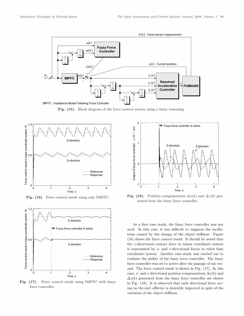
Fig. (15). Block diagram of the force control system using a fuzzy reasoning.

0.5

Force

contr

ol res

ult in

base

coord

inate

syste

m N

1.0

X-direction

Z-direction

0

ReferenceResponse

0 1 2 3 4Time s

Fig. (16). Force control result using only IMFFC.

Force

contr

ol res

ult in

base

coord

inate

syste

m N

X-direction

Z-direction

Fuzzy force controller is active

0.5

1.0

0

ReferenceResponse

0 1 2 3 4Time s

Fig. (17). Force control result using IMFFC with fuzzy

force controller.

1

2

X-direction Z-direction

0

Fuzzy force controller is active

Outpu

t of fu

zzy f

orce c

ontro

ller

x 10

-4 mm

-1 0 1 2 3 4Time s

Fig. (18). Position compensations ∆x(k) and ∆z(k) gen-

erated from the fuzzy force controller.

As a first case study, the fuzzy force controller was not

used. In this case, it was difficult to suppress the oscilla-

tions caused by the change of the object stiffness. Figure

(16) shows the force control result. It should be noted that

the z-directional contact force in sensor coordinate system

is represented by x- and z-directional forces in robot base

coordinate system. Another case study was carried out to

evaluate the ability of the fuzzy force controller. The fuzzy

force controller was set to active after the passage of one sec-

ond. The force control result is shown in Fig. (17). In this

case, x- and z-directional position compensations ∆x(k) and

∆z(k) generated from the fuzzy force controller are shown

in Fig. (18). It is observed that each directional force act-

ing on the end -effector is desirably improved in spite of the

variation of the object stiffness.


Table 3. Simulation condition for acquiring teaching signals

Approaching velocity 18.4 mm/s

Desired contact force Fd 20 N

Stiffness of object 100, 500, 1000 N/m,

Desired damping of IMFFC Bd Trial and error

IN CASE OF NEURAL NETWORKNeural Network Force Control

Next, a force control system using a neural network (NN)

is presented to realize a desirable contact motion with high

speed response characteristics between a manipulator and

an environment. For example, the PC-based controller used

in the robot sander provides API (Application Programming

Interface) functions to control the position/orientation of the

arm tip with velocity commands [11]. Making good use of

the API functions, it is expected that if the control method

is described by a velocity-based command, then the method

can be easily applied to actual open architectural industrial

robots. Thus, if the neural network considered in this sec-

tion is made up of a model whose output is the quantity of

velocity, it will be used for the actual robot with the open

architectural controller without difficulty.

First of all, in order to acquire teaching signals, we con-

sider a contact control problem as shown in Fig. (13), in

which the tip of the PUMA560 comes in contact with the

environment from normal direction with a low speed and

then it is stabilized with a desired contact force by using

the IMFFC. The desired teaching signals are ideal responses

without overshoots and oscillations, which are suitable for

training patterns of the neural network. Simulations on con-

tact motion were repeatedly conducted with trial and er-

ror under the condition tabulated in Table 3. Through the

simulation with an environmental stiffness Km=1000 N/m,

a desirable response of force error sefz(k) = Fdz − Fz(k)

as shown in Fig. (19) was obtained along normal direc-

tion. Note that s denotes the sensor coordinate system andsef (k) is composed of [sefx(k) sefy(k) sefz(k)]T . In this case,

the z-directional velocity sz(k) yielding at the arm tip was

shown in Fig. (20). The results given by Figs. (19) and

(20) are one pattern of teaching signals for input and out-

put, respectively. Other two teaching signals for inputs are

∆sefz = sefz(k)−sefz(k−1) and sz(k−1), respectively. Sim-

ilarly, other teaching signals with the condition of Km=500

and 100 N/m were respectively obtained through simula-

tions.

As an example, we design a neural network model with

three inputs and one output in z-direction of sensor coordi-

nate system. The three inputs are the force error sefz(k),

its increment ∆sefz(k) and velocity of arm tip sz(k − 1) in

z-direction of sensor coordinate system as illustrated in Fig.

(13). Also, the output of NN is the velocity sznn(k). In

0

Forc

e er

ror

N

0 0.2 0.4 0.6 0.8 1.0 1.2Time s

5

10

Km = 1000 N/m

Fig. (19). A desirable force response sEfz(k) for a teaching

signal obtained through simulation.

0 0.2 0.4 0.6 0.8 1.0 1.20

Veloc

ity c

m/s

Time s

4

5

3

2

1

Km = 1000 N/m

Fig. (20). Velocity of arm tip sz(k), which is the teaching

signal of output of neural network.

order to learn the ideal contact motion, a four-layered recur-

rent neural network composed of an input layer, two hidden

layers and an output layer is used as shown in Fig. (21).

The two hidden layers have twenty units respectively. The

input to the hidden layers or the output layer is a weighted

sum of the previous layer. The sum is squashed into ±0.5

by the following nonlinear activation function:

f(X) =1

1 + exp(−X)− 0.5 (31)

The input/output relation of each unit is given by

Xi,l =

n∑j=1

wi,lj,l−1oj,l−1 (32)

where Xi,l is the state of ith unit in lth layer. wi,lj,l−1 is the

interconnection weight between the ith unit in lth layer and

the jth unit in (l− 1)th layer. oj,l−1 is the output of the jth

unit in (l − 1)th layer. n is the number of units in (l − 1)th

layer. The neural network was trained by the back prop-

agation algorithm to learn the mapping between force and

velocity responses without overshoot and oscillation. The


)(ke fzs

)(ke fzs∆ )(kznns&

)1( −kznns&

Input

Output

Input layer

2nd layer 3rd layer

Outputlayer

Fig. (21). Neural network for dynamics learning of contact

motion.

0 100 200Trial number

0.04

Erro

r fun

ctio

n E

0.02

0

0.03

0.01

Fig. (22). Learning history of error function E.

learning was iterated until error function E became small

sufficiently. Figure (22) shows the learning history, in which

the error function E is calculated by

E =

N∑k=1

|sz(k) − sznn(k)|N

(33)

where N is the number of the training patter, i.e., total dis-

crete time in the simulation. After the learning process, the

NN could give an output as shown in Fig. (23) similar to

the teaching signal.

Simulation of Neural Network Force Controller

Figure (25) shows the block diagram of the force con-

trol system using the learned neural network, in which the

output from the neural network is feedforwardly added to

the output of the IMFFC. A force control result in case of

Km=1000 N/m is shown in Fig. (24). It is observed that

the response is improved and the raising time is shortened by

using the learned neural network. In this case, IMFFC+NN,

NN only and IMFFC only generate manipulated variables as

shown in Fig. (26), rspectively. The neural network feedfor-

wardly generates desired manipulated variables. However,

if the environment had a stiffer dynamics than the learned

environment, then the contact characteristics tended to be-

come worse. In such a case, an adaptability against to un-

learned environment should be considered. As an example,

0 0.2 0.4 0.6 0.8 1.0 1.20

Veloc

ity c

m/s

Time s

4

5

3

2

1

Km = 1000 N/m

Fig. (23). Output sznn(k) generated from the learned neu-

ral network.

0 0.5 1.0 1.5Time s

Forc

e er

ror

N

0

5

10

Fig. (24). An example of force control result by feedfor-

wardly using the learned NN.

the feedback error learning of neural network will be effective

to carry out an on-line learning [12], [13].

CONCLUSIONSIn this article, a simulation technique of velocity-based

discrete-time control system for open architectural industrial

robots has been presented by giving and combining exam-

ples of intelligent controls such as genetic algorithms, fuzzy

control and neural network. In order to develop a novel

control system for an open architectural industrial robot, it

is required from the points of view concerning safety, cost

and easiness to preliminarily examine and evaluate the char-

acteristics and performance. In such a case, the proposed

simulation technique will be useful.

It is important and required to realize a simple and ac-

curate simulation environment for industrial robots with an

open architectural controller. When a computer is used to

control an industrial robot, the control law is generally rep-

resented by a discrete-time control system. For this reason,

it has been considered on how to simulate and evaluate the

discrete-time control system which will be implemented into

an open architectural industrial robot. In order to carry

out a simulation with a robotic dynamic model, we have


IMFFC

PUMA560

+

+

_

ResolvedAcceleration

Controller

Neural NetworkForce Controller

z1

t∆1

z1

t∆1

+( )kfx&

( )kx

( )krx

( )krx&

( )krx&&

τ

( )kF

dF+

z1

t∆1

+

( )knnx&

+

+

_

_

_

( )ke

( )ke∆

: Current position



z1

t∆1( )kx& +

_

Fig. (25). Block diagram of the force control system using a neural network.

0 0.5 1.0 1.5Time s

0

Veloc

ity c

m/s

4.5

3.0

1.5

Veloc

ity c

m/s

Veloc

ity c

m/s

0

0

3.0

2.0

1.0

0.2

0.4

0.6

Output of IMFCC+NN

Output of NN

Output of IMFCC

Fig. (26). The upper, middle and lower figures show the

outputs from IMFFC+NN, NN only and IMFFC only,

respectively.

shown the scheme in detail which transforms the velocity-

based manipulated variables into joint driving torques. The

effectiveness and promise have been also demonstrated by

simulations using a dynamic model of the PUMA560 ma-

nipulator. Preliminary evaluation of various new control

approaches will be realized easily and safely for industrial

robots with an open architectural controller due to the pro-

posed simulation technique.

REFERENCES[1] C. Chen, M.M. Trivedi, C.R. Bidlack, “Simulation and animation

of sensor-driven robots,” IEEE Trans. on Robotics and Automa-

tion, vol. 10, no. 5, pp. 684–704, 1994.

[2] F. Benimeli, V. Mata, F. Valero, “A comparison between direct

and indirect dynamic parameter identification methods in indus-

trial robots,” Robotica, vol. 24, no. 5, pp. 579–590, 2006.

[3] P. Corke, “A Robotics Toolbox for MATLAB,” IEEE Robotics &

Automation Magazine, vol. 3, no. 1, pp. 24–32, 1996.

[4] P. Corke, “MATLAB Toolboxes: robotics and vision for students

and teachers,” IEEE Robotics & Automation Magazine, vol. 14,

no. 4, pp. 16–17, 2007.

[5] J.Y.S. Luh, M.H. Walker, R.P.C. Paul, “Resolved acceleration

control of mechanical Manipulator,” IEEE Trans. on Automatic

Control, vol. 25, no. 3, pp. 468–474, 1980.

[6] F. Nagata, K. Kuribayashi, K. Kiguchi and K. Watanabe, “Sim-

ulation of fine gain tuning using genetic algorithms for model-

based robotic servo controllers,” Procs. of the IEEE Int. Symp.

on Computational Intelligence in Robotics and Automation, pp.

196–201, 2007.

[7] F. Nagata, I. Okabayashi, M. Matsuno, et al., “Fine gain tun-

ing for model-based robotic servo controllers using genetic algo-

rithms,” Procs. of the 13th Int. Conf. on Advanced Robotics, pp.

987–992, 2007.

[8] N. Hogan, “Impedance control: An approach to manipulation:

Part I - Part III,” Trans. of the ASME, Journal of Dynamic

Systems, Measurement and Control, vol. 107, pp. 1–24, 1985.

[9] F. Nagata, K. Watanabe, S. Hashino, et al., “Polishing robot using

a joystick controlled teaching system,” Procs. of the IEEE Int.

Conf. on Industrial Electronics, Control and Instrumentation,

pp. 632–637, 2000.

[10] J.J. Craig, Introduction to ROBOTICS —Mechanics and Control

Second Edition—, Reading MA: Addison Wesley Publishing Co.,

1989.

[11] F. Nagata, Y. Kusumoto, Y. Fujimoto and K. Watanabe,

“Robotic sanding system for new designed furniture with free-

formed surface,” Robotics and Computer-Integrated Manufactur-

ing, vol. 23, no. 4, pp. 371–379, 2007.

[12] M. Kawato, “The feedback-error-learning neural network for su-

pervised motor learning,” Advanced Neural Computers, Elsevier

Amsterdam, pp. 365–373, 1990.

[13] J. Nakanishi, S. Schaal, “Feedback error learning and nonlinear

adaptive control,” Neural Networks, vol. 17, no. 10, pp. 1453–

1465, 2004.


Received: June 12, 2008 Revised: June 30, 2008 Accepted: July 10, 2008

c⃝Fusaomi Nagata; Licensee Bentham Open.

This is an open accees article licenced under the terms of the Creative Commons Attribution Non-Commercial License

(http://creativecommons.org/licensesby-nc/3.0/) which permits unrestricted, non-commercial use, distribution and reproduction in any medium, provided the

work is properly cited.

Documents

Simulation Technique of Velocity-Based Discrete-time ... · discrete-time control system for an open architectural industrial robot, it is required from the points of view concerning