Simulation of Wind Generation in Resource Adequacy Assessments Mary Johannis, Bonneville Power Administration

Simulation of Wind Generation in Resource Adequacy

Assessments

Mary Johannis, Mary Johannis,

Bonneville Power AdministrationBonneville Power Administration

November 14, 2008 PNW Resource Adequacy Technical Committee Meeting

2

Topics of Discussion

• Backcast of Wind Generation

• Correlation of Wind Generation and Temperature

• Creation of Synthetic Wind Generation Records

– Correlated with temperature– Exhibiting observed persistence

• Do recent Extreme Temperature Events Capture Historical Variability?

Backcast of Wind Generation This topic and others investigated by

Ben Kujala, BPA Student Intern


4

Backcast Prerequisites

• Borismetrics Contract identified problem with trying to backcast wind generation using off-site anemometer data: no unique function

• In order to backcast, prerequisites include:– Long-term clean anemometer data record, on-site if possible– Good correlation between anemometer data & wind generation


5

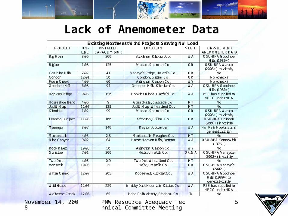
Lack of Anemometer Data

Existing Northwest Wind Projects Serving NW Load PROJECT ON-

LINE INSTALLED

CAPACITY (MW) LOCATION STATE ON-SITE WIND

ANEMOMETER DATA Big Horn 8/06 200 Bickleton, Klickitat Co. WA OSU-BPA Goodnoe

Hills (1980+) Biglow 1/08 125 Wasco, Sherman Co. OR OSU-BPA Wasco

(2005+) in vicinity Combine Hills 2/07 41 Vansycle Ridge, Umatilla Co. OR No Condon 12/01 50 Condon, Gilliam Co. OR No (check) Foote Creek 4/99 60 Arlington, Carbon Co. WY No (check) Goodnoe Hills 6/08 94 Goodnoe Hills, Klickitat Co. WA OSU-BPA Goodnoe

Hills (1980+) Hopkins Ridge 9/05 150 Hopkins Ridge, Garfield Co. WA PSE has supplied to

NPCC under NDA Horseshoe Bend 4/06 9 Great Falls, Cascade Co. MT No Judith Gap 12/05 135 Judith Gap, Wheatland Co. MT No Klondike 1/02 99 Wasco, Sherman Co. OR OSU-BPA Wasco

(2005+) in vicinity Leaning Juniper 11/06 100 Arlington, Gilliam Co. OR OSU-BPA Chinook

(2006+) in vicinity Marengo 8/07 140 Dayton, Columbia WA No (PSE Hopkins is in

general vicinity) Martinsdale 4/05 2.8 Martinsdale, Meagher Co. MT No Nine Canyon 9/02 64 Horse Heaven Hills, Benton WA OSU-BPA Kennewick

(1976+) Rock River 10/03 50 Arlington, Carbon Co. WY No Stateline 7/01 300 Helix, Umatilla Co. OR/WA OSU-BPA Vansycle

(2002+) in vicinity Two Dot 4/05 0.9 Two Dot, Wheatland Co. MT No Vansycle 10/98 25 Helix, Umatilla Co. OR OSU-BPA Vansycle

(2002+) White Creek 12/07 205 Roosevelt, Klickitat Co. WA OSU-BPA Goodnoe

Hills (1980+) in general vicinity

Wild Horse 12/06 229 Whisky Dick Mountain, Kittitas Co. WA PSE has supplied to NPCC under NDA

Wolverine Creek 12/05 65 Idaho Falls vicinity, Bingham Co. ID No


6

Vansycle Backcast Case Study

• Vansycle has an anemometer on-site– ½ mile from the nearest generator– 6 miles from the furthest generator

• Wind speed data is available in 10 minute intervals for period• Scada data is available in 5 minute intervals for period• Vansycle Backcast should be doable

– Relatively long-term Generation Record – Relatively clean Anemometer Record

• Wind Turbine Power Characteristics:– Cut-in wind speed 4 m/s (8.9 mph)– Nominal wind speed 15 m/s (33.6 mph)– Stop wind speed 25 m/s (55.9 mph)


7

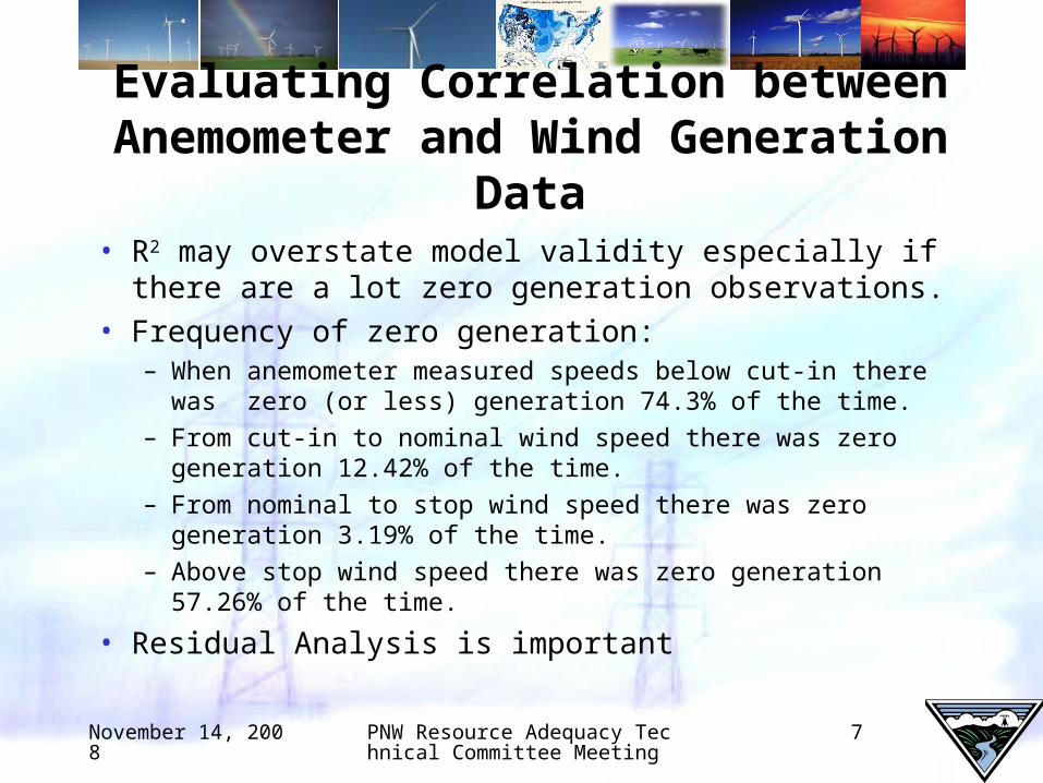
Evaluating Correlation between Anemometer and Wind Generation Data

• R2 may overstate model validity especially if there are a lot zero generation observations.

• Frequency of zero generation:– When anemometer measured speeds below cut-in there

was zero (or less) generation 74.3% of the time.– From cut-in to nominal wind speed there was zero

generation 12.42% of the time.– From nominal to stop wind speed there was zero generation

3.19% of the time.– Above stop wind speed there was zero generation 57.26%

of the time.

• Residual Analysis is important


8

Developing the Model

• Model needs to respect wind turbine characteristics– If wind speed < 8.95 mph then adjusted wind capacity = 0– If wind speed >= 8.95 and <= 33.6 then wind capacity (rolling

average) is correlated with a function of (wind speed – 8.95)/(33.55-8.95)

– If wind speed > 33.6 and <= 55.9 then adjusted wind capacity = 1

– If wind speed > 55.9 then adjusted wind capacity = 0

• Cubic polynomial regression was applied to the adjusted wind speed (after centering) and used to predict the rolling capacity– Initial R2 = .7266 after excluding zero generation– Residual analysis indicates problem with initial model


9

Residual Analysis

• Residuals are the difference between the observation and the proposed model (fits).– Ideally residuals should be evenly scattered about zero for

any given wind speed. That is the model should pass through the “middle” of the observed data.

– Rather than simply looking at the model, it is sometimes easier to examine a residual plot where residuals are plotted against various other variables. A good model will have evenly scattered residuals that are roughly in a rectangular region about the zero line in a residual plot.


10

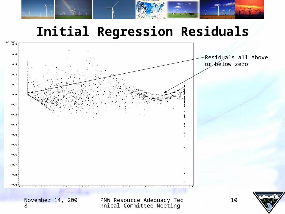
Initial Regression Residuals

Residuals all above or below zero


11

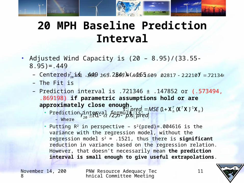
20 MPH Baseline Prediction Interval

• Adjusted Wind Capacity is (20 – 8.95)/(33.55-8.95)=.449– Centered is .449 - .284 = .165

– The Fit is

– Prediction interval is .721346 ± .147852 or (.573494, .869198) if parametric assumptions hold or are approximately close enough.

• Prediction interval formula is:– Where

• Putting R2 in perspective – s2{pred}=.004616 is the variance with the regression model, without the regression model s2 = .1521, thus there is significant reduction in variance based on the regression relation. However, that doesn’t necessarily mean the prediction interval is small enough to give useful extrapolations.

721346.22107.202817.609.1465.165.165.165.1ˆ 3220 TY

predspntY ;2/12̂0 ))(1( 12

hTT

hMSEpreds XXXX


12

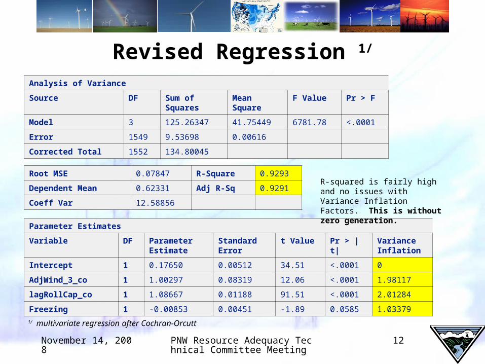
Revised Regression 1/

Analysis of Variance

Source DF Sum ofSquares

MeanSquare

F Value Pr > F

Model 3 125.26347 41.75449 6781.78 <.0001

Error 1549 9.53698 0.00616

Corrected Total 1552 134.80045

Root MSE 0.07847 R-Square 0.9293

Dependent Mean 0.62331 Adj R-Sq 0.9291

Coeff Var 12.58856

Parameter Estimates

Variable DF ParameterEstimate

StandardError

t Value Pr > |t| VarianceInflation

Intercept 1 0.17650 0.00512 34.51 <.0001 0

AdjWind_3_co 1 1.00297 0.08319 12.06 <.0001 1.98117

lagRollCap_co 1 1.08667 0.01188 91.51 <.0001 2.01284

Freezing 1 -0.00853 0.00451 -1.89 0.0585 1.03379

R-squared is fairly high and no issues with Variance Inflation Factors. This is without zero generation.

1/ multivariate regression after Cochran-Orcutt


13

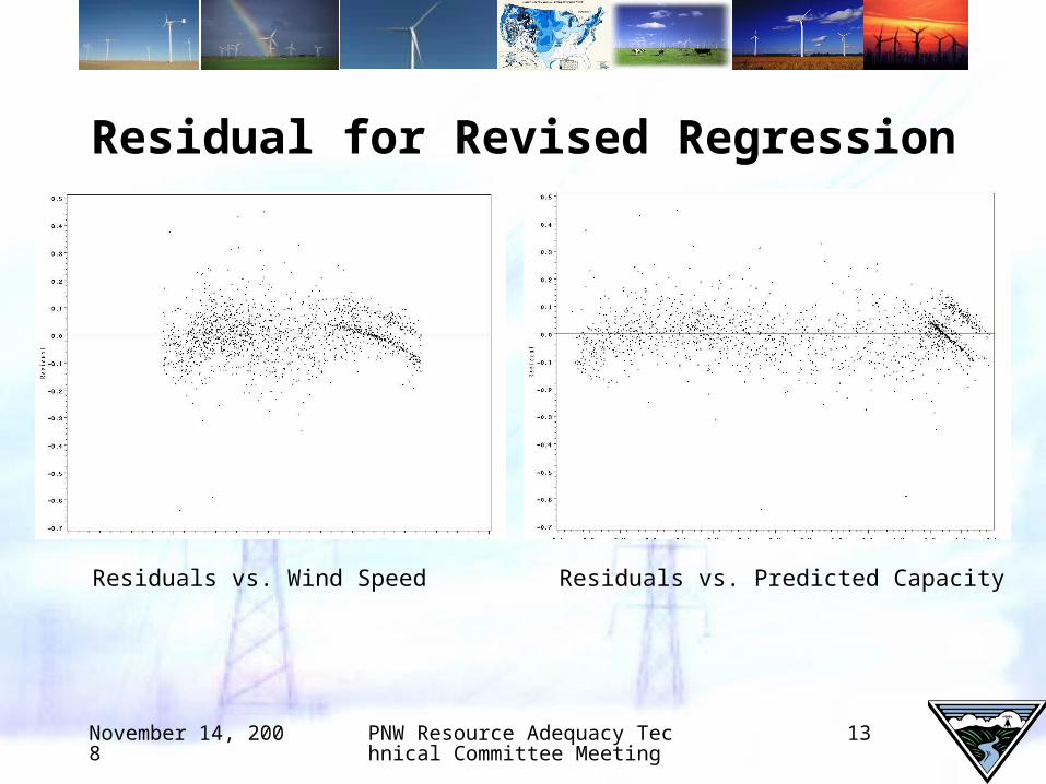
Residual for Revised Regression

Residuals vs. Wind Speed Residuals vs. Predicted Capacity


14

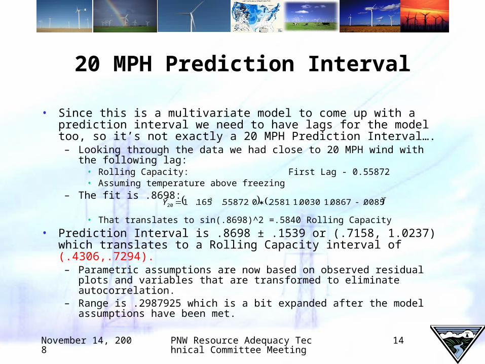
20 MPH Prediction Interval

• Since this is a multivariate model to come up with a prediction interval we need to have lags for the model too, so it’s not exactly a 20 MPH Prediction Interval….

– Looking through the data we had close to 20 MPH wind with the following lag:

• Rolling Capacity: First Lag - 0.55872• Assuming temperature above freezing

– The fit is .8698:

• That translates to sin(.8698)^2 =.5840 Rolling Capacity

• Prediction Interval is .8698 ± .1539 or (.7158, 1.0237) which translates to a Rolling Capacity interval of (.4306,.7294).

– Parametric assumptions are now based on observed residual plots and variables that are transformed to eliminate autocorrelation.

– Range is .2987925 which is a bit expanded after the model assumptions have been met.

TY 0085.0867.10030.12581.055872.165.1ˆ 320


15

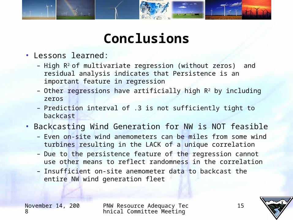
Conclusions• Lessons learned:

– High R2 of multivariate regression (without zeros) and residual analysis indicates that Persistence is an important feature in regression

– Other regressions have artificially high R2 by including zeros– Prediction interval of .3 is not sufficiently tight to backcast

• Backcasting Wind Generation for NW is NOT feasible – Even on-site wind anemometers can be miles from some

wind turbines resulting in the LACK of a unique correlation – Due to the persistence feature of the regression cannot use

other means to reflect randomness in the correlation– Insufficient on-site anemometer data to backcast the entire

NW wind generation fleet

Correlation of Wind Generation and Temperature


17

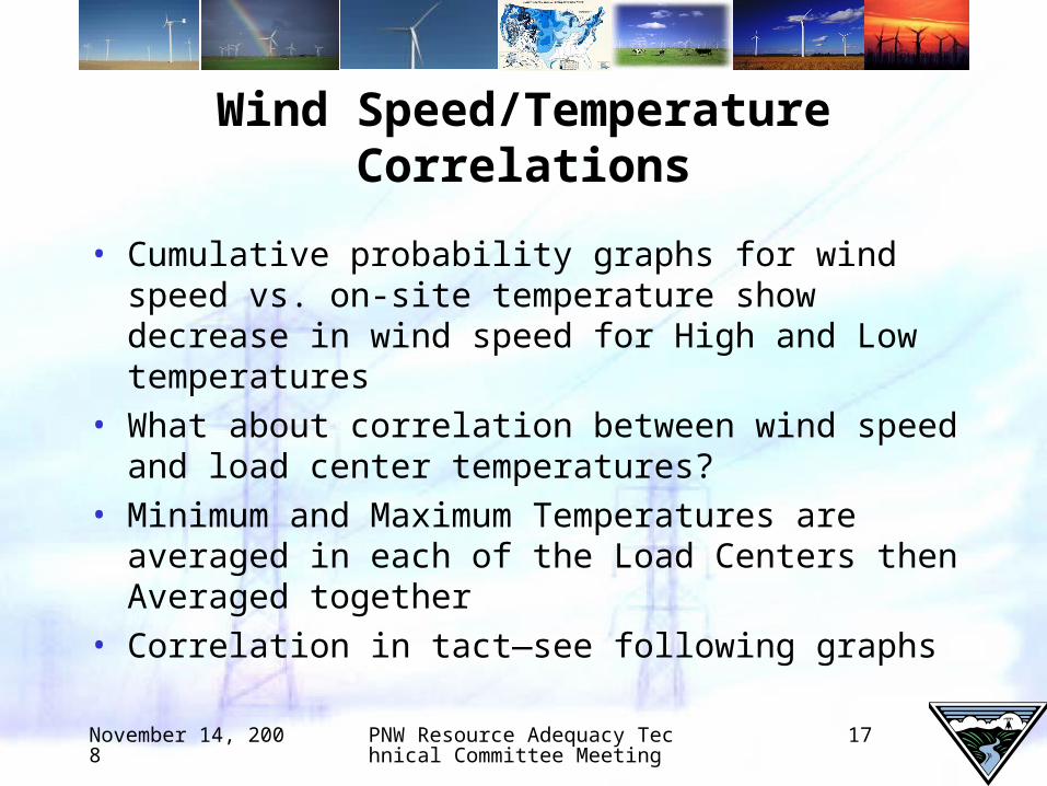
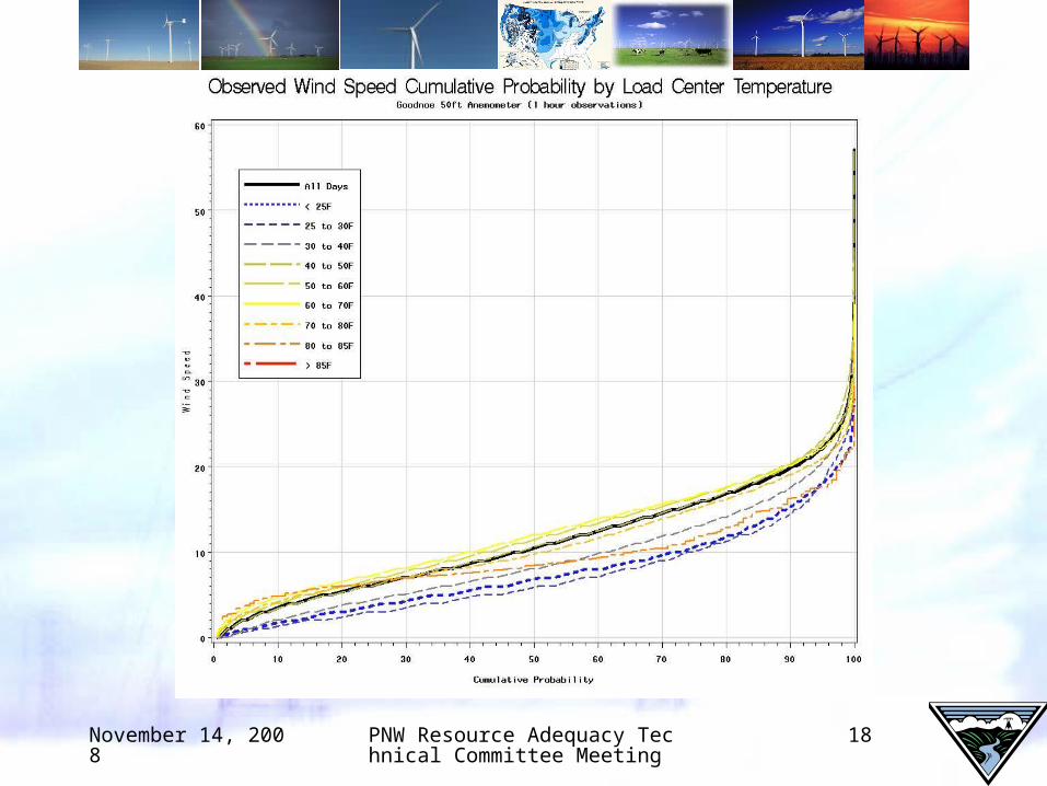
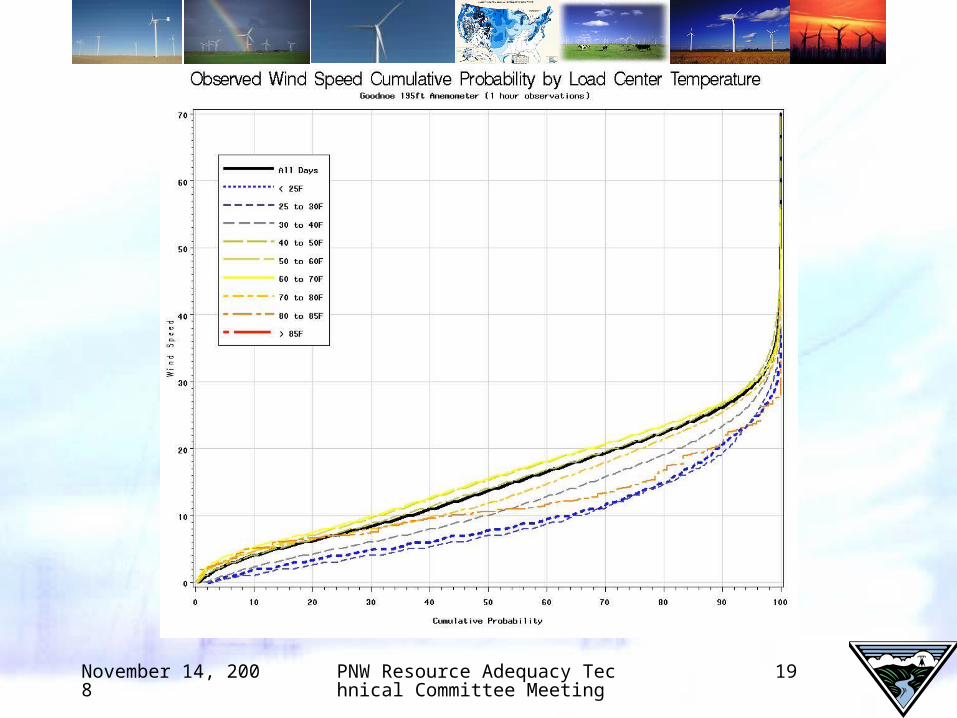
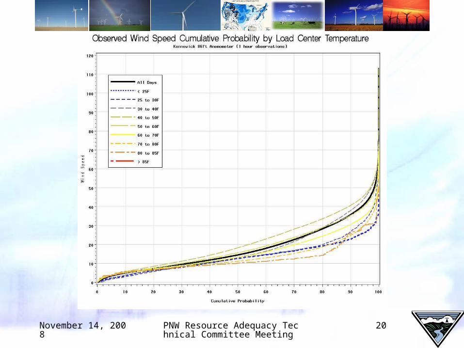
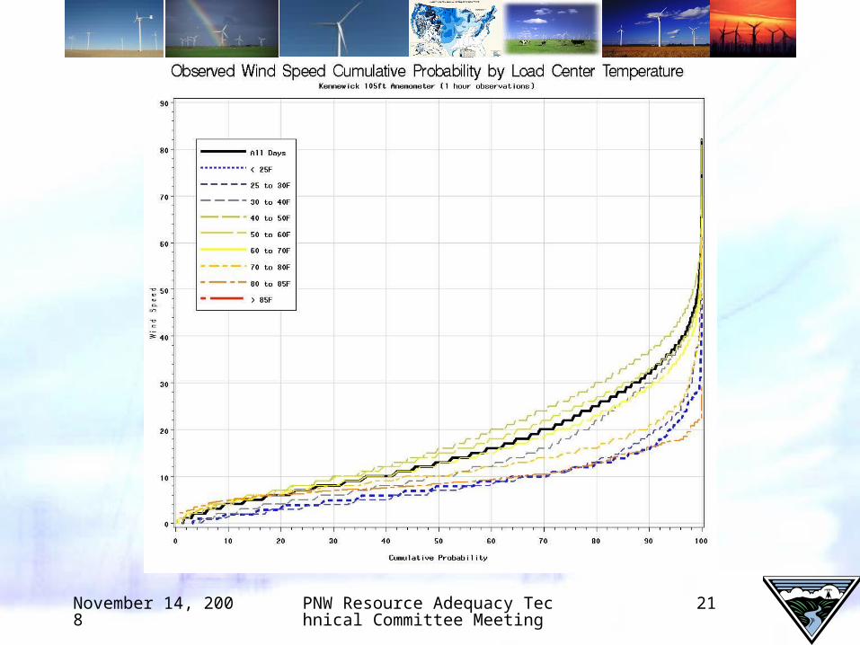
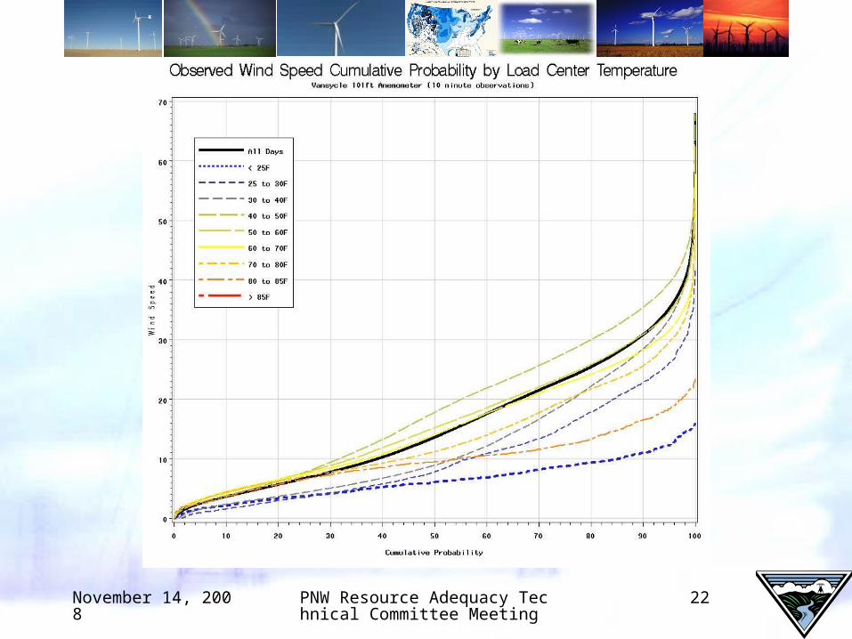
Wind Speed/Temperature Correlations

• Cumulative probability graphs for wind speed vs. on-site temperature show decrease in wind speed for High and Low temperatures

• What about correlation between wind speed and load center temperatures?

• Minimum and Maximum Temperatures are averaged in each of the Load Centers then Averaged together

• Correlation in tact—see following graphs


18


19


20


21


22

Recommendation to Create Synthetic Wind Generation Records Correlated

with Historic Temperature


24

Creating Valid Long-term Synthetic Data Records

• Kennewick Presentation at 8/14/08 Forum Wind Assessment Team Meeting provides support that short-term wind attributes ~ long-term wind attributes historical wind generation can be used to create synthetic data that mimics long-term record

• Synthetic data should have the same, or at least a very similar distribution as observed data.

• Synthetic data should preserve the structure of observed data.– For instance, with wind generation data it is important to maintain

persistence.

• Purely Synthetic data should not lead to fundamentally different conclusions than the observed data would warrant.


25

Creating a Synthetic Historical Record with the Question in Mind

• What questions are the studies trying to answer?– Is wind generation related to hydro generation?– Is wind generation related to demand because both are

correlated to temperature?– Is there seasonality in wind generation?– How can wind uncertainty be correctly modeled in the tails,

i.e. when Loss of Load may occur?

• The problem with using something other than a time span as the selection criteria is that wind generation is a time series, so to break apart the observations and not maintain order means that there must be some other way to maintain the structure of the data


26

What is the Kth Nearest Neighbor Method?

• Given a time series of size N, a possible approach to creating synthetic data is to randomly select a single or two consecutive of the N observations then select the third based on how “close” the lag(s) for the selected observation are to the randomly selected observation(s).– For example, if we select two hours where the capacity is .3

the first and .4 the second, then look through the data and pull from observations that have capacities that are close to .3 for the observation 2 hours prior and .4 for the hour prior.

– Creating a subset of the K “closest” observations to draw from maintains the structure that is expected in the time series.


27

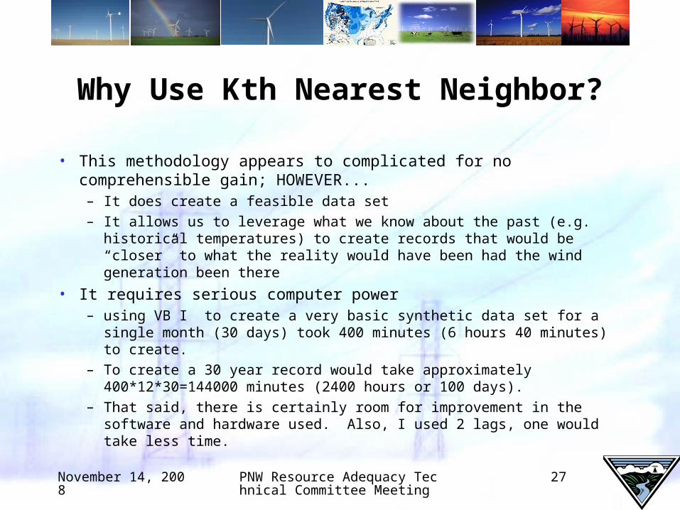
Why Use Kth Nearest Neighbor?

• This methodology appears to complicated for no comprehensible gain; HOWEVER...– It does create a feasible data set

– It allows us to leverage what we know about the past (e.g. historical temperatures) to create records that would be “closer” to what the reality would have been had the wind generation been there

• It requires serious computer power– using VB I to create a very basic synthetic data set for a single

month (30 days) took 400 minutes (6 hours 40 minutes) to create.

– To create a 30 year record would take approximately 400*12*30=144000 minutes (2400 hours or 100 days).

– That said, there is certainly room for improvement in the software and hardware used. Also, I used 2 lags, one would take less time.


28

Comparability

• All synthetic data sets should be compared to one another. Creating data sets without some sort of baseline comparison is definitely not recommended. They should be consistent with actual observations and other synthetic data. The improvements should be seen in specific areas such as load comparison where there is a rational explanation for simulated effects.


29

Develop Proof of Concept of Kth Nearest Neighbor Synthetic Data

Methodology

• BPA is pursuing Contract with contract with Portland State University to provide statistical review of methodology– Ben Kujala will develop proof of concept

• Long-term Alternatives– If Proof of Concept successful, create long-term

Synthetic Wind Generation set that is correlated to temperature for partial or entire data set

– Explore other Synthetic Data Alternatives

An Examination of Historical Temperature Extremes

BPA Investigation

by Peggy Miller

10/16/08


31

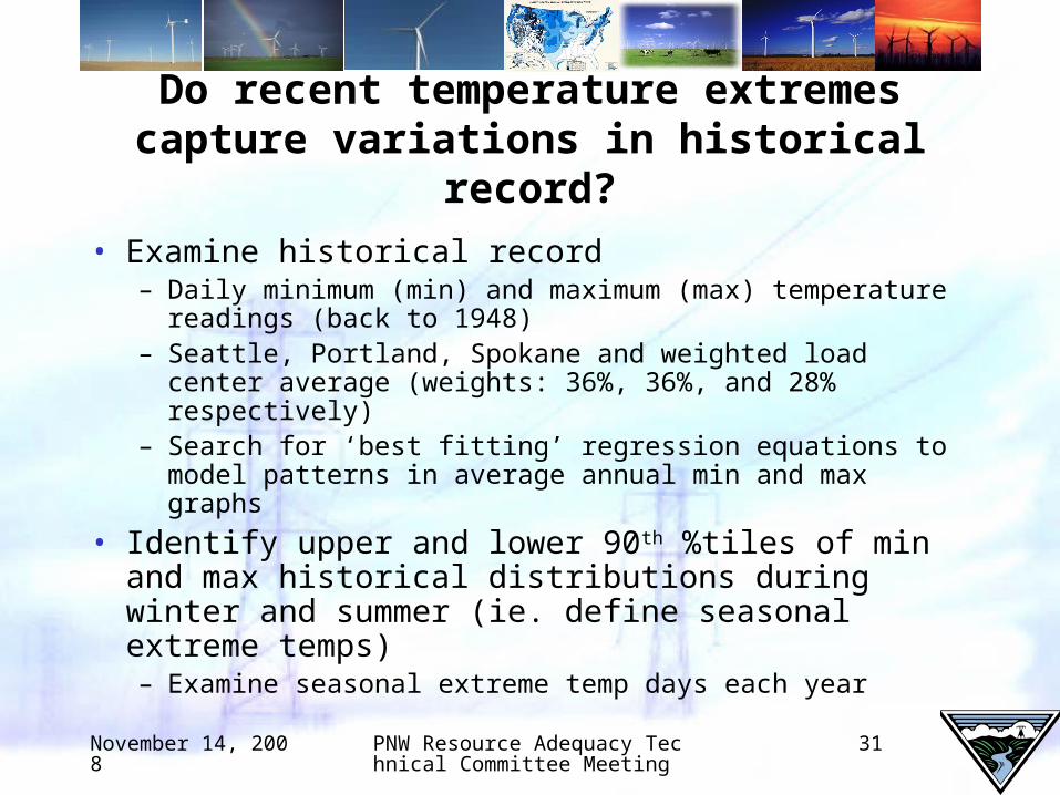
Do recent temperature extremes capture variations in historical record?

• Examine historical record– Daily minimum (min) and maximum (max) temperature

readings (back to 1948)– Seattle, Portland, Spokane and weighted load center

average (weights: 36%, 36%, and 28% respectively)– Search for ‘best fitting’ regression equations to model

patterns in average annual min and max graphs

• Identify upper and lower 90th %tiles of min and max historical distributions during winter and summer (ie. define seasonal extreme temps)– Examine seasonal extreme temp days each year


32

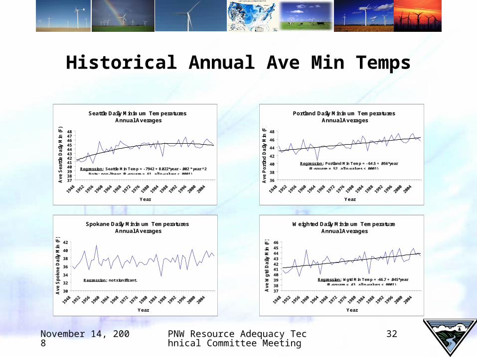
Historical Annual Ave Min Temps

Seattle Daily Minimum Temperatures Annual Averages

373839404142434445464748

Year

Av

e S

ea

ttle

Da

ily

Min

(F

)

Regression: Seattle Min Temp = - 7942 + 8.022*year - .002 * year ^2 Note: non-linear, (R-square = .61 , all p-values < .0001)

Portland Daily Minimum Temperatures Annual Averages

36

38

40

42

44

46

48

Year

Av

e P

ort

lnd

Da

ily

Min

(F

)

Regression: Portland Min Temp = - 64.5 + .056*year (R-square = .52 , all p-values < .0001)

Spokane Daily Minimum Temperatures Annual Averages

30

32

34

36

38

40

42

Year

Av

e S

po

kn

e D

ail

y M

in (

F)

Regression: not significant.

Weighted Daily Minimum Temperature Annual Averages

37383940414243444546

Year

Av

e W

gtd

Da

ily

Min

(F

)

Regression: Wgtd Min Temp = -46.7 + .045*year (R-square = .43 , all p-values < .0001)


33

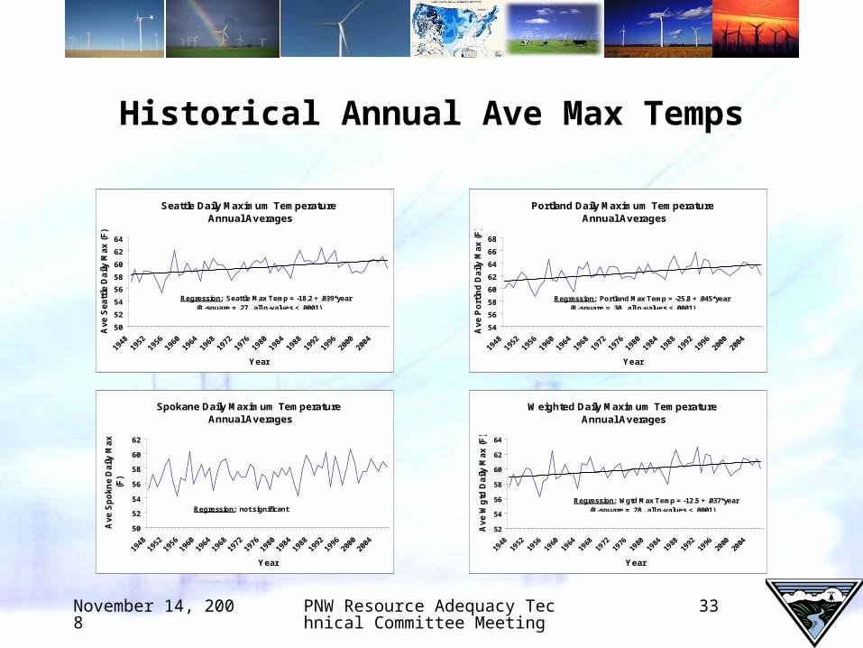
Historical Annual Ave Max Temps

Seattle Daily Maximum Temperature Annual Averages

50

52

54

56

58

60

62

64

Year

Av

e S

ea

ttle

Da

ily

Ma

x (

F)

Regression: Seattle Max Temp = -18.2 + .039*year (R-square = .27 , all p-values < .0001)

Portland Daily Maximum Temperature Annual Averages

54

56

58

60

62

64

66

68

Year

Av

e P

ort

lnd

Da

ily

Ma

x (

F)

Regression: Portland Max Temp = -25.8 + .045*year (R-square = .30 , all p-values < .0001)

Spokane Daily Maximum Temperature Annual Averages

50

52

54

56

58

60

62

Year

Av

e S

po

kn

e D

ail

y M

ax

(F

)

Regression: not significant

Weighted Daily Maximum Temperature Annual Averages

52

54

56

58

60

62

64

Year

Av

e W

gtd

Da

ily

Ma

x (

F)

Regression: Wgtd Max Temp = -12.5 + .037*year (R-square = .28 , all p-values < .0001)


34

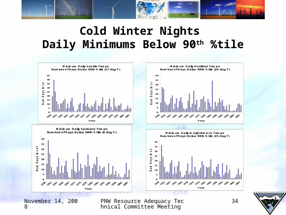
Cold Winter Nights Daily Minimums Below 90th %tile

Minimum Daily Seattle Temps Number of Days Below 90th %tile (27 deg F)

0

5

10

15

20

25

30

35

40

45

Year

Nu

m D

ay

s in

Le

ft T

ail

Minimum Daily Portland Temps Number of Days Below 90th %tile (26 deg F)

0

5

10

15

20

25

30

35

40

Year

Nu

m D

ay

s in

Le

ft T

ail

Minimum Daily Spokane Temps Number of Days Below 90th %tile (8 deg F)

0

5

10

15

20

25

30

35

40

Year

Nu

m D

ay

s in

Le

ft T

ail

Minimum Daily Weighted Ave Temps Number of Days Below 90th %tile (23 deg F)

0

5

10

15

20

25

30

35

40

Year

Nu

m D

ay

s in

Le

ft T

ail


35

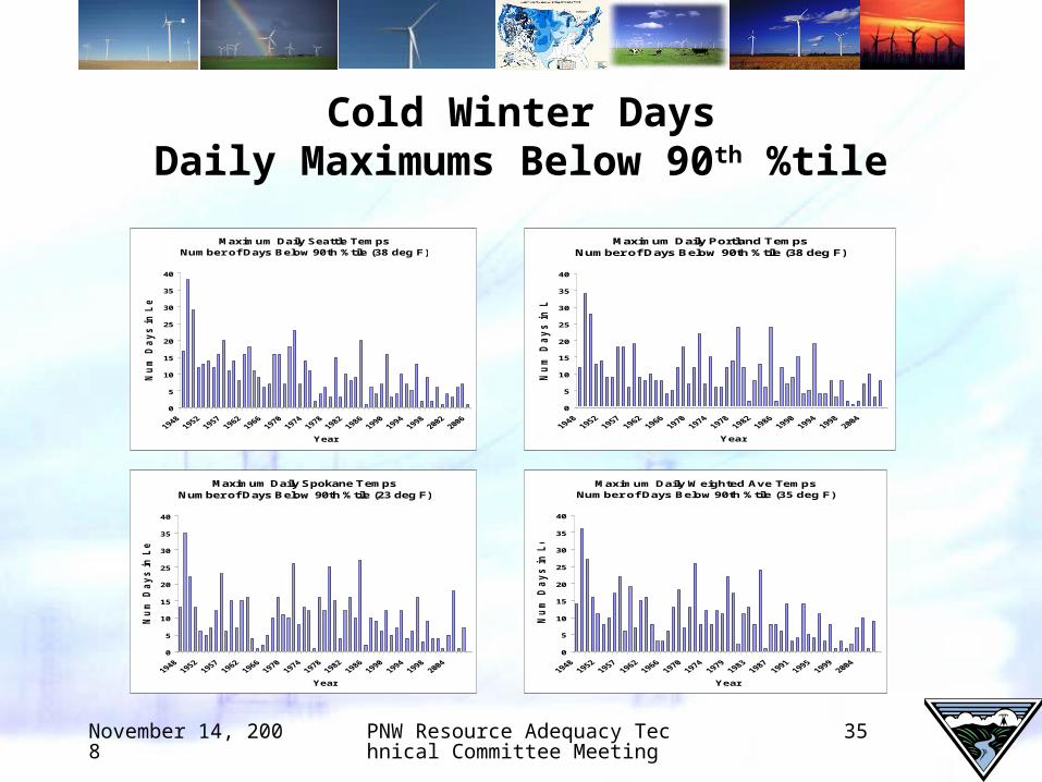
Cold Winter DaysDaily Maximums Below 90th %tile

Maximum Daily Seattle Temps Number of Days Below 90th %tile (38 deg F)

0

5

10

15

20

25

30

35

40

Year

Nu

m D

ay

s in

Le

ft T

ail

Maximum Daily Portland Temps Number of Days Below 90th %tile (38 deg F)

0

5

10

15

20

25

30

35

40

Year

Nu

m D

ay

s in

Le

ft T

ail

Maximum Daily Spokane Temps Number of Days Below 90th %tile (23 deg F)

0

5

10

15

20

25

30

35

40

Year

Nu

m D

ay

s in

Le

ft T

ail

Maximum Daily Weighted Ave Temps Number of Days Below 90th %tile (35 deg F)

0

5

10

15

20

25

30

35

40

Year

Nu

m D

ay

s in

Le

ft T

ail


36

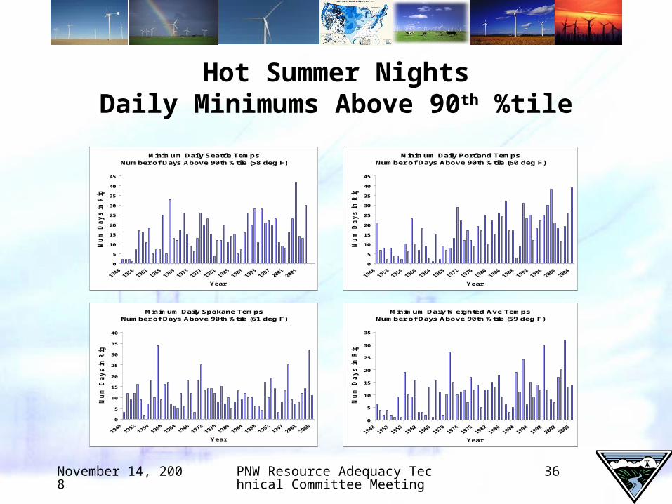
Hot Summer NightsDaily Minimums Above 90th %tile

Minimum Daily Seattle Temps Number of Days Above 90th %tile (58 deg F)

0

5

10

15

20

25

30

35

40

45

Year

Nu

m D

ay

s in

Rig

ht

Ta

il

Minimum Daily Portland Temps Number of Days Above 90th %tile (60 deg F)

0

5

10

15

20

25

30

35

40

45

Year

Nu

m D

ay

s in

Rig

ht

Ta

il

Minimum Daily Spokane Temps Number of Days Above 90th %tile (61 deg F)

0

5

10

15

20

25

30

35

40

Year

Nu

m D

ay

s in

Rig

ht

Ta

il

Minimum Daily Weighted Ave Temps Number of Days Above 90th %tile (59 deg F)

0

5

10

15

20

25

30

35

Year

Nu

m D

ay

s in

Rig

ht

Ta

il


37

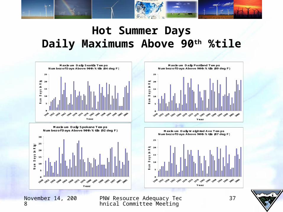
Hot Summer DaysDaily Maximums Above 90th %tile

Maximum Daily Seattle Temps Number of Days Above 90th %tile (84 deg F)

0

5

10

15

20

25

Year

Nu

m D

ay

s in

Rig

ht

Ta

il

Maximum Daily Portland Temps Number of Days Above 90th %tile (89 deg F)

0

5

10

15

20

25

Year

Nu

m D

ay

s in

Rig

ht

Ta

il

Maximum Daily Spokane Temps Number of Days Above 90th %tile (92 deg F)

0

5

10

15

20

25

30

Year

Nu

m D

ay

s in

Rig

ht

Ta

il

Maximum Daily Weighted Ave Temps Number of Days Above 90th %tile (87 deg F)

0

5

10

15

20

25

Year

Nu

m D

ay

s in

Rig

ht

Ta

il


38

Conclusions

• The data suggest that the average annual mins and maxes have significantly increased about 2.4 °F (~0.04 °F * 60 years) since 1948 in Portland, Seattle and on a weighted load center basis. (Note that these temp increases are not necessarily due to global warming. Variables such as population, urbanization, albedo, possible long term cyclical nature, etc. were not included in the model)

• Overall, temp extremes during recent years do capture historical variations in temp extremes, but are slightly warmer than the 60-year mean in keeping with the trend of increasing temperature

Documents

Simulation of Wind Generation in Resource Adequacy Assessments Mary Johannis, Bonneville Power Administration