Simulation of Ultrasound Pulse Propagation in Lossy Media

114 ieee transactions on ultrasonics, ferroelectrics, and frequency control, vol. 45, no. 1, january 1998

Simulation of Ultrasound Pulse Propagation inLossy Media Obeying a Frequency Power Law

Ping He, Member, IEEE

Abstract—A method is proposed to simulate the propa-gation of a broadband ultrasound pulse in a lossy mediumwhose attenuation exhibits a power law frequency depen-dence. Using a bank of Gaussian filters, the broadband pulseis first decomposed into narrowband components. The ef-fects of the attenuation and dispersion are then appliedto each component based on the superposition principle.When the bandwidth of each component is narrow enough,these effects can be evaluated at the center frequency ofthe component, resulting in a magnitude reduction, a con-stant phase angle lag, and a relative time delay. The accu-racy of the proposed method is tested by comparing themodel-produced pulses with the experimentally measuredpulses using two different phantoms. The first phantom hasan attenuation function which exhibits a nearly linear fre-quency dependence. The second phantom has an attenua-tion function which exhibits a nearly quadratic frequencydependence. In deriving the dispersion from the measuredattenuation, a nearly local model and a time causal modelare used. For linear attenuation, the two models convergeand both predict accurately the waveform of the transmit-ted pulse. For nonlinear attenuation, the time causal modelis found more accurate than the nearly local model in pre-dicting the waveform of the transmitted pulse.

I. Introduction

When a broadband ultrasound pulse passes through alayer of medium, the waveform of the pulse changes

as a result of the attenuation and dispersion of themedium. Many media, including soft tissues, have beenobserved to have an attenuation function which increaseswith frequency. As a result, the higher frequency compo-nents of the pulse are attenuated more than the lower fre-quency components. After passing through the layer, thetransmitted pulse is not just a scaled down version of theincident pulse, but will have a different shape. Dispersionrefers to the phenomenon that the phase velocity of a prop-agating wave also changes with frequency [1]. Dispersioncauses additional change in the waveform of the propa-gating pulse because the wave components with differentfrequencies travel at different speeds. An understanding ofthe interaction of ultrasound with tissue medium in boththe time and frequency domains and the ability to de-termine the waveform change of propagating ultrasoundpulses should be valuable in the design of array trans-ducer and in quantitative ultrasound tissue characteriza-tion [2], [3].

Manuscript received December 10, 1996; accepted July 14, 1997.The author is with the Department of Biomedical and Human

Factors Engineering, Wright State University, Dayton, OH 45435 (e-mail: [email protected]).

The classical method for predicting the waveformchange of a signal passing through a medium relies on theimpulse response of the system. According to the theoryof linear systems, the output signal is the convolution ofthe input signal and the system’s impulse response. Theimpulse response can be obtained by taking the inverseFourier transform of the frequency response of the systemwhich generally takes the following form:

H(ω) = A(ω)e−jθ(ω)x = e−α(ω)xe−jxω/Vp(ω) (1)

where H(ω) is the frequency response, A(ω) is the magni-tude function, θ(ω) is the phase angle per unit distance,α(ω) is the attenuation function, Vp(ω) is the phase veloc-ity, and x is the thickness of the layer. If α(ω) and Vp(ω)are both known, the impulse response of the medium canfirst be synthesized and the output signal can then be de-termined.

The attenuation function of many soft tissues have beenextensively measured and tabled [4]. In general, tissue at-tenuation can be expressed by a power law function [5], [6]:

α(ω) = α0ωy (2)

where α0 and y are tissue-dependent attenuation parame-ters. On the other hand, the dispersion has been foundvery small and difficult to measure directly [5]. As afirst approximation, one may ignore the dispersion andassume a linear-with-frequency phase term [7]. Unfortu-nately, the impulse response of such a system is not causal[2]. To ensure the causality while avoiding a direct mea-surement of the dispersion, Gurumurthy and Arthur [2]proposed a minimum-phase model for a layer of tissue.For a minimum-phase system, the attenuation and phaseof its frequency response are related to each other by a pairof Hilbert transforms [8]. Because of this property, the en-tire frequency response, and the impulse response as well,of the layer can be obtained based on the knowledge ofthe medium’s attenuation only. When such an approach isused to model a layer of tissue, two problems arise. Firstof all, the Hilbert transform relations between the atten-uation and dispersion are defined in such a way that, inorder to obtain the value of one of them at any single fre-quency, it is necessary to know the values of the other atall frequencies [2], [8]. Tissue attenuation, however, is usu-ally measured over a limited frequency range, e.g. from 1to 10 MHz. The first problem, therefore, is to validate theassumption that the values of α at all other frequenciescan be correctly extrapolated from the measured values.The second problem is related to a so-called Paley-Wiener

0885–3010/97$10.00 c© 1998 IEEE

he: ultrasound pulse propagation in lossy media 115

condition which states that for A(ω) to be the Fourierspectrum of a causal function, a necessary and sufficientcondition is that the following inequality is satisfied [8]:

∞∫−∞

| lnA(ω)|1 + ω2 dw <∞ (3)

For most soft tissues, the attenuation function α defined in(2) is approximately a linear function of frequency (y = 1)[5]. Some tissues, however, have been observed to exhibita nonlinear frequency dependence [9], [10]. In general, theexponent y for soft tissues is in the range 1 ≤ y ≤ 2.For such an attenuation function, the Paley-Wiener con-dition is not satisfied. To overcome this problem, Guru-murthy and Arthur [2] modified the high frequency be-havior of the attenuation function by imposing a high-frequency limit that beyond which the magnitude functiondoes not go to zero faster than an exponential. Kuc [3] cir-cumvented the problem associated with the Paley-Wienercondition by implementing the minimum phase model inthe discrete-time domain. In such a case, the folding fre-quency (1/2 of the sampling frequency) becomes the nat-ural high-frequency limit. The phase function between thezero and folding frequencies is derived from the attenua-tion function within the same frequency range by employ-ing the Hilbert transform in the discrete-time domain. Be-yond the folding frequency, however, it is assumed thatthe magnitude function is mirror symmetric with respectto the folding frequency (i.e., the attenuation function de-creases with frequency and reaches zero at the samplingfrequency) so that the impulse response is a real function.While both approaches avoid the problem associated withthe Paley-Wiener condition, the assumption made on theattenuation function in a certain frequency range remainsto be validated.

In this paper, we present an alternative method fordetermining the output signal that does not invoke theimpulse response of the system and does not need theassumption about the attenuation beyond a certain fre-quency. The method is based on the superposition prin-ciple for a linear system: if we consider the input signalas a combination of many narrowband components, eachpropagating in the medium at a certain speed (dispersion)and subjecting to a frequency-dependent attenuation, theoutput signal can then be obtained by regrouping the in-dividually transmitted components. In implementing themethod, the attenuation is measured over the frequencyrange of the input signal, and the dispersion is derivedfrom the measured attenuation over the same frequencyrange. In determining the dispersion from the attenua-tion, two models are used. The first model, which wasderived by O’Donnell et al. [11], does not explicitly em-phasize the dependence of the degree of dispersion on theexponent y in (2). The second model was proposed by Sz-abo [12], [13] more recently. According to Szabo’s model,the degree of dispersion is strongly dependent upon theexponent y: when y = 1, the dispersion is maximized;when y approaches 2, the dispersion vanishes. The accu-

racy of the proposed method will be tested by comparingthe model-produced pulses with the experimentally mea-sured pulses using two different phantoms. The first phan-tom has an attenuation function which exhibits a nearlylinear frequency dependence. The second phantom has anattenuation function which exhibits a nearly quadratic fre-quency dependence. Because the two models used to derivethe dispersion from attenuation deviate from each otherwhen y > 1, the transmitted waveforms predicted by thetwo models are expected to show noticeable difference forthe second phantom. By comparing the measured and pre-dicted waveforms, the relative accuracy of the two modelsalso can be tested.

II. Method

A. Decomposition of a Broadband Pulse

Biological tissues appear to respond linearly to diag-nostic ultrasound [2]. For such a linear system, the su-perposition principle holds. Consequently, the propagationof a broadband ultrasound pulse can be studied by firstdecomposing the pulse into many wave components, andthen analyzing the propagation of each wave component.There are different ways to decompose a signal. Classi-cal Fourier transform decomposes a signal into sinusoidalwaveforms, each having a single frequency and oscillatingforever. Modern wavelet analysis decomposes a signal intoa set of wavelet components by dilating and translatinga mother wavelet. Wavelet analysis is more efficient thanFourier analysis when the signal is dominated by transientbehavior or discontinuities. Because the ultrasound pulsestypically used in B-scan imaging are relatively smooth, wechoose to use a simpler time-frequency representation inthat each wave component will have a finite constant band-width which is narrow enough so that the attenuation anddispersion can be evaluated at a single frequency.

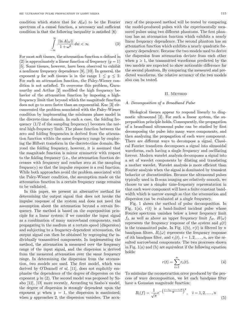
Fig. 1 shows the method of pulse decomposition. InFig. 1(a), r(t) is a band-limited incident pulse whoseFourier spectrum vanishes below a lower frequency limitfL as well as above an upper frequency limit fH . H(ω)represents the frequency response of the system and g(t)is the transmitted pulse. In Fig. 1(b), r(t) is filtered by nbandpass filters. Bi(ω) represents the frequency responseof ith bandpass filter, and ri(t), i = 1, 2, . . . , n, are the re-sulted narrowband components. The two processes shownin Fig. 1(a) and (b) are equivalent if the following equationholds:

r(t) =n∑i=1

ri(t). (4)

To minimize the reconstruction error produced by the pro-cess of wave decomposition, we let each bandpass filterhave a Gaussian magnitude function:

Bi(f) =1√πe−(f−fL−(i−1)B

B

)2

, i = 1, 2, . . . , n(5)


Fig. 1. (a) A broadband pulse r(t) passes through a layer of mediumhaving a frequency response of H(ω) and produces a transmittedpulse g(t). (b) Based on the superposition principle, r(t) is first de-composed into n narrowband components by a bank of bandpassfilters. Each component ri(t) then passes through the same mediumand the transmitted signals are added together to produce g(t).

where B = (fH − fL)/(n− 1). Fig. 2 shows the individualBi(f) of the bandpass filters which are actually used inthis study. In Fig. 2, fL = 0.5 MHz, fH = 5.5 MHz, n =11, and B = 0.5 MHz (the choice of n and B will bediscussed later). Fig. 2 also shows that the combined filterresponse

∑iBi(f) which is very close to a constant one

in the midband (from 1.5 MHz to 4.5 MHz, it is within1±0.00011) and drops 2.1 dB at fL and fH . We will showlater (in Fig. 5) that by using these Gaussian filters, thereconstruction error associated with the process of wavedecomposition is negligible.

B. Transformation of the System Response

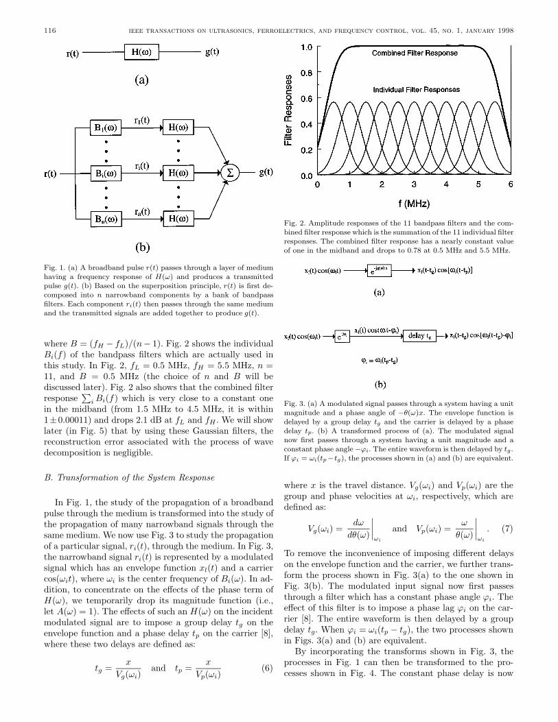
In Fig. 1, the study of the propagation of a broadbandpulse through the medium is transformed into the study ofthe propagation of many narrowband signals through thesame medium. We now use Fig. 3 to study the propagationof a particular signal, ri(t), through the medium. In Fig. 3,the narrowband signal ri(t) is represented by a modulatedsignal which has an envelope function xl(t) and a carriercos(ωit), where ωi is the center frequency of Bi(ω). In ad-dition, to concentrate on the effects of the phase term ofH(ω), we temporarily drop its magnitude function (i.e.,let A(ω) = 1). The effects of such an H(ω) on the incidentmodulated signal are to impose a group delay tg on theenvelope function and a phase delay tp on the carrier [8],where these two delays are defined as:

tg =x

Vg(ωi)and tp =

x

Vp(ωi)(6)

Fig. 2. Amplitude responses of the 11 bandpass filters and the com-bined filter response which is the summation of the 11 individual filterresponses. The combined filter response has a nearly constant valueof one in the midband and drops to 0.78 at 0.5 MHz and 5.5 MHz.

Fig. 3. (a) A modulated signal passes through a system having a unitmagnitude and a phase angle of −θ(ω)x. The envelope function isdelayed by a group delay tg and the carrier is delayed by a phasedelay tp. (b) A transformed process of (a). The modulated signalnow first passes through a system having a unit magnitude and aconstant phase angle−ϕi. The entire waveform is then delayed by tg.If ϕi = ωi(tp−tg), the processes shown in (a) and (b) are equivalent.

where x is the travel distance. Vg(ωi) and Vp(ωi) are thegroup and phase velocities at ωi, respectively, which aredefined as:

Vg(ωi) =dω

dθ(ω)

∣∣∣∣ωi

and Vp(ωi) =ω

θ(ω)

∣∣∣∣ωi

. (7)

To remove the inconvenience of imposing different delayson the envelope function and the carrier, we further trans-form the process shown in Fig. 3(a) to the one shown inFig. 3(b). The modulated input signal now first passesthrough a filter which has a constant phase angle ϕi. Theeffect of this filter is to impose a phase lag ϕi on the car-rier [8]. The entire waveform is then delayed by a groupdelay tg. When ϕi = ωi(tp − tg), the two processes shownin Figs. 3(a) and (b) are equivalent.

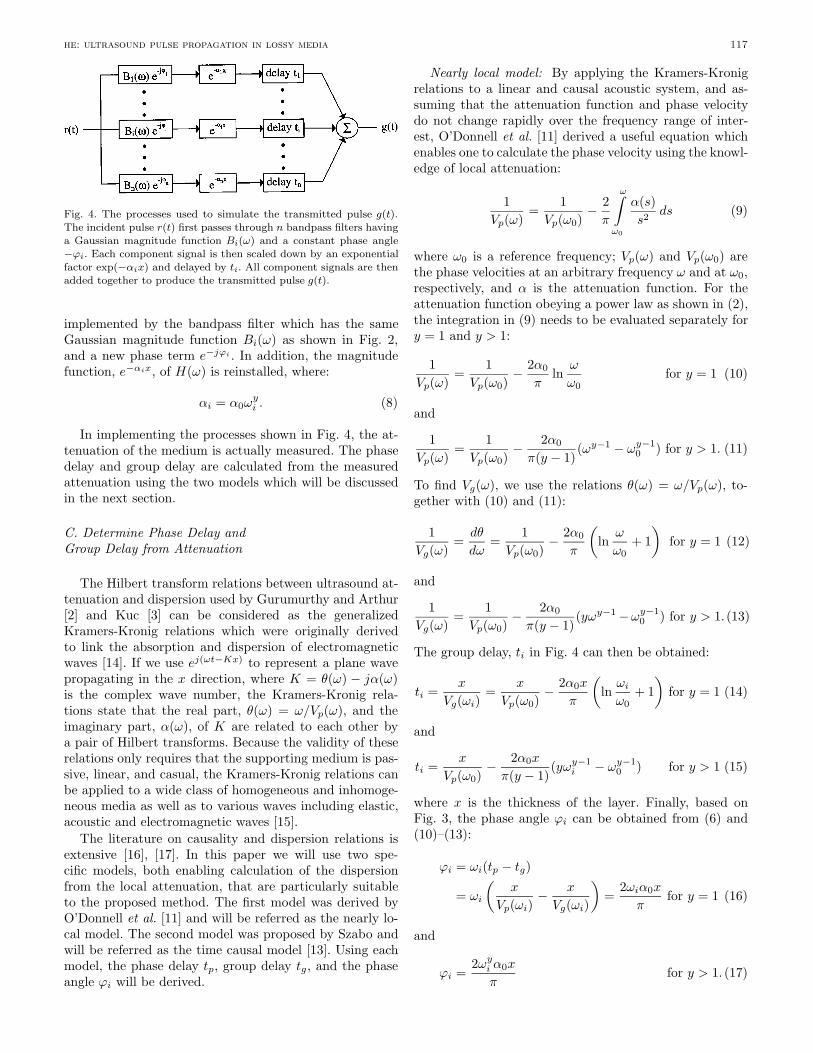
By incorporating the transforms shown in Fig. 3, theprocesses in Fig. 1 can then be transformed to the pro-cesses shown in Fig. 4. The constant phase delay is now


Fig. 4. The processes used to simulate the transmitted pulse g(t).The incident pulse r(t) first passes through n bandpass filters havinga Gaussian magnitude function Bi(ω) and a constant phase angle−ϕi. Each component signal is then scaled down by an exponentialfactor exp(−αix) and delayed by ti. All component signals are thenadded together to produce the transmitted pulse g(t).

implemented by the bandpass filter which has the sameGaussian magnitude function Bi(ω) as shown in Fig. 2,and a new phase term e−jϕi . In addition, the magnitudefunction, e−αix, of H(ω) is reinstalled, where:

αi = α0ωyi . (8)

In implementing the processes shown in Fig. 4, the at-tenuation of the medium is actually measured. The phasedelay and group delay are calculated from the measuredattenuation using the two models which will be discussedin the next section.

C. Determine Phase Delay andGroup Delay from Attenuation

The Hilbert transform relations between ultrasound at-tenuation and dispersion used by Gurumurthy and Arthur[2] and Kuc [3] can be considered as the generalizedKramers-Kronig relations which were originally derivedto link the absorption and dispersion of electromagneticwaves [14]. If we use ej(ωt−Kx) to represent a plane wavepropagating in the x direction, where K = θ(ω) − jα(ω)is the complex wave number, the Kramers-Kronig rela-tions state that the real part, θ(ω) = ω/Vp(ω), and theimaginary part, α(ω), of K are related to each other bya pair of Hilbert transforms. Because the validity of theserelations only requires that the supporting medium is pas-sive, linear, and casual, the Kramers-Kronig relations canbe applied to a wide class of homogeneous and inhomoge-neous media as well as to various waves including elastic,acoustic and electromagnetic waves [15].

The literature on causality and dispersion relations isextensive [16], [17]. In this paper we will use two spe-cific models, both enabling calculation of the dispersionfrom the local attenuation, that are particularly suitableto the proposed method. The first model was derived byO’Donnell et al. [11] and will be referred as the nearly lo-cal model. The second model was proposed by Szabo andwill be referred as the time causal model [13]. Using eachmodel, the phase delay tp, group delay tg, and the phaseangle ϕi will be derived.

Nearly local model: By applying the Kramers-Kronigrelations to a linear and causal acoustic system, and as-suming that the attenuation function and phase velocitydo not change rapidly over the frequency range of inter-est, O’Donnell et al. [11] derived a useful equation whichenables one to calculate the phase velocity using the knowl-edge of local attenuation:

1Vp(ω)

=1

Vp(ω0)− 2π

ω∫ω0

α(s)s2 ds (9)

where ω0 is a reference frequency; Vp(ω) and Vp(ω0) arethe phase velocities at an arbitrary frequency ω and at ω0,respectively, and α is the attenuation function. For theattenuation function obeying a power law as shown in (2),the integration in (9) needs to be evaluated separately fory = 1 and y > 1:

1Vp(ω)

=1

Vp(ω0)− 2α0

πln

ω

ω0for y = 1 (10)

and

1Vp(ω)

=1

Vp(ω0)− 2α0

π(y − 1)(ωy−1 − ωy−1

0 ) for y > 1. (11)

To find Vg(ω), we use the relations θ(ω) = ω/Vp(ω), to-gether with (10) and (11):

1Vg(ω)

=dθ

dω=

1Vp(ω0)

− 2α0

π

(ln

ω

ω0+ 1)

for y = 1 (12)

and

1Vg(ω)

=1

Vp(ω0)− 2α0

π(y − 1)(yωy−1−ωy−1

0 ) for y > 1. (13)

The group delay, ti in Fig. 4 can then be obtained:

ti =x

Vg(ωi)=

x

Vp(ω0)− 2α0x

π

(lnωiω0

+ 1)

for y = 1 (14)

and

ti =x

Vp(ω0)− 2α0x

π(y − 1)(yωy−1

i − ωy−10 ) for y > 1 (15)

where x is the thickness of the layer. Finally, based onFig. 3, the phase angle ϕi can be obtained from (6) and(10)–(13):

ϕi = ωi(tp − tg)

= ωi

(x

Vp(ωi)− x

Vg(ωi)

)=

2ωiα0x

πfor y = 1 (16)

and

ϕi =2ωyi α0x

πfor y > 1. (17)


Time causal model: Szabo [12] derived a time do-main expression of causality analogous in function to theKramers-Kronig relations in the frequency domain. Basedon this new time casual model, an equation similar to (11)was derived which enables one to calculate the phase veloc-ity from the attenuation values near a reference frequencyω0 [13]. The original form of equation 27 shown in Szabo’spaper [13] is recasted here as:

1Vp(ω)

=1

Vp(ω0)+ α0 tan

(yπ

2

)(ωy−1 − ωy−1

0 ).(18)

By comparing (11) and (18), one finds a simple procedureto transform the results obtained by the nearly local modelto the corresponding results predicted by the time casualmodel. That is to perform the following conversion:

2π(y − 1)

−→ − tan(yπ

2

). (19)

When y approaches 1 from the right side (y > 1),

2π(y − 1)

∼= − tan(yπ

2

). (20)

As a result, when y = 1, the two models converge and thetime causal model will predict the same results as shown in(12), (14), and (16). When y > 1, the two models deviatefrom each other, and the time causal model predicts thefollowing results:

1Vg(ω)

=1

Vp(ω0)+ α0 tan

(yπ

2

)(yωy−1 − ωy−1

0 )(21)

ti =x

Vp(ω0)+ α0x tan

(yπ

2

)(yωy−1

i − ωy−10 )

(22)

ϕi = −(y − 1)ωyi α0x tan(yπ

2

). (23)

III. Measurement and Simulation Results

To test the processes shown in Fig. 4 for predicting thewaveform of the transmitted pulse, two phantoms are usedin through-transmission measurements. The first phan-tom is a Plexiglas block, which has an almost linear-with-frequency attenuation. The speed of sound of the materialis measured as 2736 m/s. The second phantom, which ismanufactured by ATS Laboratories (Bridgeport, CT), ismade of a special rubber material having a speed of soundof 1465 m/s. The ATS phantom material has an attenua-tion function which exhibits a highly nonlinear frequencydependence. The thickness of both phantoms is 8.0 cm.

Two transducers are situated 25 cm apart in a watertank and are aligned properly. The transmitting trans-ducer (Panametrics V309, 13-mm aperture) has a nom-inal center frequency of 5.0 MHz and a focal length of89 mm. The receiving transducer (Panametrics V382, 13-mm aperture) has a nominal center frequency of 3.5 MHz

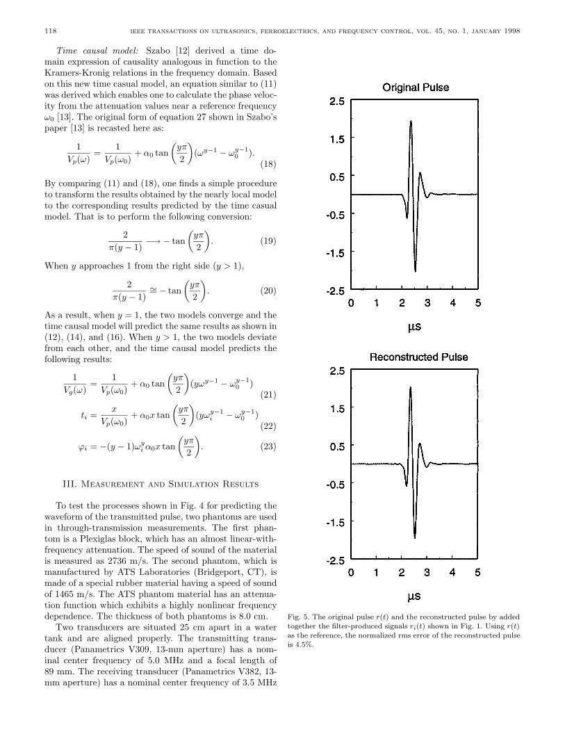
Fig. 5. The original pulse r(t) and the reconstructed pulse by addedtogether the filter-produced signals ri(t) shown in Fig. 1. Using r(t)as the reference, the normalized rms error of the reconstructed pulseis 4.5%.


and a focal length of 76 mm. The pulser/receiver used inthe study is Panametrics 5052PR. The RF data ampli-fied by the receiver are digitized by a SONY/TEK 390ADprogrammable digitizer which has a 10-bit resolution anda sampling frequency of 60 MHz. With only a water pathbetween the two transducers, the pulse waveform receivedby the receiving transducer is recorded which will be usedas the incident pulse, r(t), in the following processes.

By taking the Fourier transform, r(t) is found tobe band limited in the frequency range of 0.5 MHz to5.5 MHz. Based on this frequency range, 11 bandpass fil-ters are used to decompose r(t) into its components (thechoice of the number of bands will be discussed later). Themagnitude transfer functions of these filters are expressedby (5) and plotted in Fig. 2. As a first test, we use the11 bandpass filters as shown in Fig. 1 to decompose theincident pulse r(t) and then reconstruct a pulse by addingthe resulted components together according to (4). Fig. 5compares the waveforms of the original pulse r(t) and thereconstructed pulse. In these plots, as well as in the restwaveform plots, the ordinate shows only the relative mag-nitude without a specific unit. We now define a normalizedroot-mean-square (rms) error which will be used through-out this paper for pulse comparisons:

ε =

√N∑i=1

[x(i)− xo(i)]2/N√N∑i=1

[xo(i)]2/N

=

√√√√√√√√N∑i=1

[x(i)− xo(i)]2

N∑i=1

[xo(i)]2 (24)

where x(i) is a sample of the signal to be tested, x0(i) isthe corresponding sample of the reference signal, and Nis the total number of samples. Using the original pulser(t) as the reference, the normalized rms error of the re-constructed pulse shown in Fig. 5 is 4.5%.

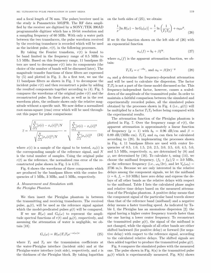
Fig. 6 shows the waveforms of three components whichare produced by the bandpass filters with the center fre-quencies of 1 MHz, 3 MHz, and 5 MHz, respectively.

A. Measurement and Simulation withthe Plexiglas Phantom

We then insert the Plexiglas phantom in betweenthe transmitting and receiving transducers. The receivedpulse, g0(t), will be used as the reference signal againstwhich the model-predicated pulses g(t) will be compared.

If we use R(ω) and G0(ω) to represent the ampli-tude spectral functions of r(t) and g0(t), respectively, andassuming the attenuation of water is negligible, we ob-tain [18]:

Go(ω) = R(ω)T1T2e−α(ω)x (25)

where T1 and T2 are the transmission coefficients atthe water-Plexiglas interface (incident side) and at thePlexiglas-water interface (exit side), respectively, and x isthe thickness of the Plexiglas block. By taking logarithm

on the both sides of (25), we obtain:

1x

[lnR(ω)− lnG0(ω)] =1x

ln(

1T1T2

)+ α0ω

y.(26)

If we fit the function shown on the left side of (26) withan exponential function

αa(f) = b0 + βfy. (27)

where αa(f) is the apparent attenuation function, we ob-tain:

T1T2 = e−xb0 , and α0 = β(2π)−y (28)

α0 and y determine the frequency-dependent attenuationand will be used to calculate the dispersion. The factorT1T2 is not a part of the tissue model discussed so far. Thisfrequency-independent factor, however, causes a scaled-down of the amplitude of the transmitted pulse. In order tomaintain a faithful comparison between the simulated andexperimentally recorded pulses, all the simulated pulsesobtained by the processes shown in Fig. 4 (i.e., g(t)) willbe multiplied by a factor T1T2 before being compared withthe experimental results.

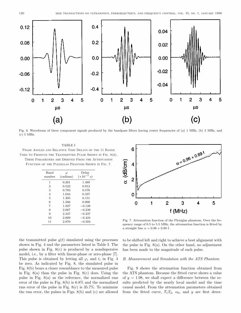
The attenuation function of the Plexiglas phantom isplotted in Fig. 7. Over the frequency range of r(t), theapparent attenuation is approximately a linear functionof frequency (y = 1) with b0 = 0.96 dB/cm and β =0.89 dB/(MHz cm). T1T2 and α0 can then be calculatedaccording to (28). In implementing the processes shownin Fig. 4, 11 bandpass filters are used with center fre-quencies of 0.5, 1.0, 1.5, 2.0, 2.5, 3.0, 3.5, 4.0, 4.5, 5.0,and 5.5 MHz, respectively. αi are determined by (8) andϕi are determined by (16). To calculate ti using (14), wechoose the midband frequency, (fL + fH)/2 = 3.0 MHz,as the reference frequency (i.e., ω0/2π), and let Vp(ω0) =2736 m/s. Because we are only interested in the relativedelays among the component signals, we let the midband(i = 6, fc = 3.0 MHz) have zero delay and express the de-lays of all other bands as the relative delays with respectto the midband. Table I lists the calculated phase anglesand relative time delays based on the measured attenua-tion of the Plexiglas phantom. A positive delay means thatthe component signal of the particular band travels slowerthan that of the reference band (midband) and a negativedelay means a faster traveling speed. As indicated by Ta-ble I, the Plexiglas has an anomalous dispersion [2]: thesignal having a higher center frequency travels faster thanthe one having a lower center frequency. To reconstructthe transmitted pulse g(t), the signal of the midband isnot changed, while the signals of all other bands are eithershifted backward (for positive delay) or forward (for nega-tive delay) with respect to the reference signal, accordingto the calculated relative delays. The shifted signals arethen added together to produce the transmitted pulse g(t).

Fig. 8 compares the simulated pulses with the measuredone. The pulse shown in Fig. 8(a) is the transmitted pulseg0(t) which is experimentally measured. Fig. 8(b) shows


Fig. 6. Waveforms of three component signals produced by the bandpass filters having center frequencies of (a) 1 MHz, (b) 3 MHz, and(c) 5 MHz.

TABLE IPhase Angles and Relative Time Delays of the 11 Bands

Used to Produce the Transmitted Pulse Shown in Fig. 8(b).

These Parameters are Derived From the Attenuation

Function of the Plexiglas Phantom Shown in Fig. 7.

Band ϕ Delaynumber (radians) (×10−7 s)

1 0.261 1.4892 0.522 0.9123 0.783 0.5764 1.044 0.3375 1.305 0.1516 1.566 0.0007 1.827 −0.1288 2.087 −0.2399 2.347 −0.33710 2.609 −0.42411 2.870 −0.503

the transmitted pulse g(t) simulated using the processesshown in Fig. 4 and the parameters listed in Table I. Thepulse shown in Fig. 8(c) is produced by a nondispersivemodel, i.e., by a filter with linear-phase or zero-phase [7].This pulse is obtained by letting all ϕi and ti in Fig. 4be zero. As indicated by Fig. 8, the simulated pulse inFig. 8(b) bears a closer resemblance to the measured pulsein Fig. 8(a) than the pulse in Fig. 8(c) does. Using thepulse in Fig. 8(a) as the reference, the normalized rmserror of the pulse in Fig. 8(b) is 6.8% and the normalizedrms error of the pulse in Fig. 8(c) is 35.7%. To minimizethe rms error, the pulses in Figs. 8(b) and (c) are allowed

Fig. 7. Attenuation function of the Plexiglas phantom. Over the fre-quency range of 0.5 to 5.5 MHz, the attenuation function is fitted bya straight line α = 0.96 + 0.89 f.

to be shifted left and right to achieve a best alignment withthe pulse in Fig. 8(a). On the other hand, no adjustmenthas been made to the magnitude of each pulse.

B. Measurement and Simulation with the ATS Phantom

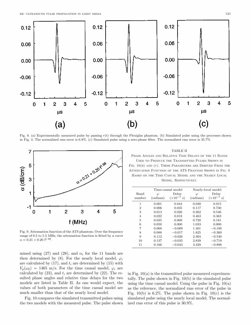
Fig. 9 shows the attenuation function obtained fromthe ATS phantom. Because the fitted curve shows a valueof y = 1.98, we shall expect a difference between the re-sults predicted by the nearly local model and the timecausal model. From the attenuation parameters obtainedfrom the fitted curve, T1T2, α0, and y are first deter-


Fig. 8. (a) Experimentally measured pulse by passing r(t) through the Plexiglas phantom. (b) Simulated pulse using the processes shownin Fig. 4. The normalized rms error is 6.8%. (c) Simulated pulse using a zero-phase filter. The normalized rms error is 35.7%.

Fig. 9. Attenuation function of the ATS phantom. Over the frequencyrange of 0.5 to 5.5 MHz, the attenuation function is fitted by a curveα = 0.21 + 0.20 f1.98.

mined using (27) and (28), and αi for the 11 bands arethen determined by (8). For the nearly local model, ϕiare calculated by (17), and ti are determined by (15) withVp(ω0) = 1465 m/s. For the time causal model, ϕi arecalculated by (23), and ti are determined by (22). The re-sulted phase angles and relative time delays for the twomodels are listed in Table II. As one would expect, thevalues of both parameters of the time casual model aremuch smaller than that of the nearly local model.

Fig. 10 compares the simulated transmitted pulses usingthe two models with the measured pulse. The pulse shown

TABLE IIPhase Angles and Relative Time Delays of the 11 Bands

Used to Produce the Transmitted Pulses Shown in

Fig. 10(b) and (c). These Parameters are Derived From the

Attenuation Function of the ATS Phantom Shown in Fig. 9

Based on the Time Casual Model and the Nearly Local

Model, Respectively.

Time-causal model Nearly-local modelBand ϕ Delay ϕ Delay

number (radians) (×10−7 s) (radians) (×10−7 s)

1 0.001 0.044 0.030 0.9152 0.006 0.035 0.117 0.7303 0.013 0.026 0.262 0.5464 0.022 0.018 0.463 0.3635 0.035 0.009 0.720 0.1816 0.050 0.000 1.033 0.0007 0.068 −0.009 1.401 −0.1808 0.088 −0.017 1.825 −0.3609 0.112 −0.026 2.304 −0.54010 0.137 −0.035 2.839 −0.71911 0.166 −0.043 3.429 −0.898

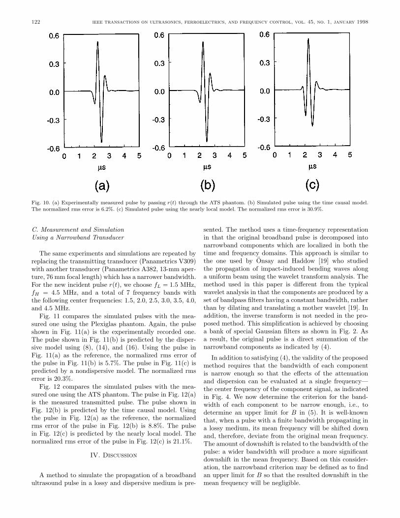
in Fig. 10(a) is the transmitted pulse measured experimen-tally. The pulse shown in Fig. 10(b) is the simulated pulseusing the time casual model. Using the pulse in Fig. 10(a)as the reference, the normalized rms error of the pulse inFig. 10(b) is 6.2%. The pulse shown in Fig. 10(c) is thesimulated pulse using the nearly local model. The normal-ized rms error of this pulse is 30.9%.


Fig. 10. (a) Experimentally measured pulse by passing r(t) through the ATS phantom. (b) Simulated pulse using the time causal model.The normalized rms error is 6.2%. (c) Simulated pulse using the nearly local model. The normalized rms error is 30.9%.

C. Measurement and SimulationUsing a Narrowband Transducer

The same experiments and simulations are repeated byreplacing the transmitting transducer (Panametrics V309)with another transducer (Panametrics A382, 13-mm aper-ture, 76 mm focal length) which has a narrower bandwidth.For the new incident pulse r(t), we choose fL = 1.5 MHz,fH = 4.5 MHz, and a total of 7 frequency bands withthe following center frequencies: 1.5, 2.0, 2.5, 3.0, 3.5, 4.0,and 4.5 MHz.

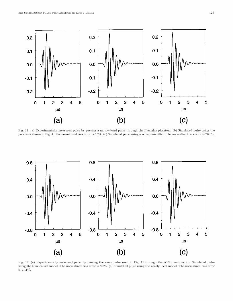
Fig. 11 compares the simulated pulses with the mea-sured one using the Plexiglas phantom. Again, the pulseshown in Fig. 11(a) is the experimentally recorded one.The pulse shown in Fig. 11(b) is predicted by the disper-sive model using (8), (14), and (16). Using the pulse inFig. 11(a) as the reference, the normalized rms error ofthe pulse in Fig. 11(b) is 5.7%. The pulse in Fig. 11(c) ispredicted by a nondispersive model. The normalized rmserror is 20.3%.

Fig. 12 compares the simulated pulses with the mea-sured one using the ATS phantom. The pulse in Fig. 12(a)is the measured transmitted pulse. The pulse shown inFig. 12(b) is predicted by the time causal model. Usingthe pulse in Fig. 12(a) as the reference, the normalizedrms error of the pulse in Fig. 12(b) is 8.8%. The pulsein Fig. 12(c) is predicted by the nearly local model. Thenormalized rms error of the pulse in Fig. 12(c) is 21.1%.

IV. Discussion

A method to simulate the propagation of a broadbandultrasound pulse in a lossy and dispersive medium is pre-

sented. The method uses a time-frequency representationin that the original broadband pulse is decomposed intonarrowband components which are localized in both thetime and frequency domains. This approach is similar tothe one used by Onsay and Haddow [19] who studiedthe propagation of impact-induced bending waves alonga uniform beam using the wavelet transform analysis. Themethod used in this paper is different from the typicalwavelet analysis in that the components are produced by aset of bandpass filters having a constant bandwidth, ratherthan by dilating and translating a mother wavelet [19]. Inaddition, the inverse transform is not needed in the pro-posed method. This simplification is achieved by choosinga bank of special Gaussian filters as shown in Fig. 2. Asa result, the original pulse is a direct summation of thenarrowband components as indicated by (4).

In addition to satisfying (4), the validity of the proposedmethod requires that the bandwidth of each componentis narrow enough so that the effects of the attenuationand dispersion can be evaluated at a single frequency—the center frequency of the component signal, as indicatedin Fig. 4. We now determine the criterion for the band-width of each component to be narrow enough, i.e., todetermine an upper limit for B in (5). It is well-knownthat, when a pulse with a finite bandwidth propagating ina lossy medium, its mean frequency will be shifted downand, therefore, deviate from the original mean frequency.The amount of downshift is related to the bandwidth of thepulse: a wider bandwidth will produce a more significantdownshift in the mean frequency. Based on this consider-ation, the narrowband criterion may be defined as to findan upper limit for B so that the resulted downshift in themean frequency will be negligible.


Fig. 11. (a) Experimentally measured pulse by passing a narrowband pulse through the Plexiglas phantom. (b) Simulated pulse using theprocesses shown in Fig. 4. The normalized rms error is 5.7%. (c) Simulated pulse using a zero-phase filter. The normalized rms error is 20.3%.

Fig. 12. (a) Experimentally measured pulse by passing the same pulse used in Fig. 11 through the ATS phantom. (b) Simulated pulseusing the time causal model. The normalized rms error is 8.8%. (c) Simulated pulse using the nearly local model. The normalized rms erroris 21.1%.


Let us consider a particular component in Fig. 4 whichhas a center frequency of fc. Because the component isproduced by passing a broadband r(t) through a narrowbandpass filter having a Gaussian spectrum, the spectrumof the resulted component is also approximately a Gaus-sian function:

S0(f) = Ae−(f−fc)2

B2 (29)

where A is the amplitude of S0(f) at the center frequencyfc, and B is the same bandwidth parameter ofBi(f) in (5).After passing through a tissue layer having an attenuationfunction α(f) = βfy and a thickness x, the spectrum ofthe attenuated pulse becomes:

S1(f) = Ae−(f−fc)2

B2 e−βfyx. (30)

We now consider the two extreme cases: y = 1 and y = 2.For y = 1, it can be shown that:

S1(f) = Ae−(f−fc)2

B2 (31)

where A is the new amplitude which is independent offrequency, and fc is the down-shifted new center frequency:

fc = fc −βB2x

2. (32)

We may then require that the relative down-shift of thecenter frequency is less than a predetermined threshold δ:

fc − fcfc

=βB2x

2fc< δ (33)

which leads to the following limitation for B:

B <

√2fcδβx

. (34)

For y = 2, it can be shown that the new spectrum of theattenuated pulse becomes:

S1(f) = Ae− (f−fc)2

(B/√

1+βB2x)2 (35)

where A is another new amplitude independent of fre-quency, and fc is the new down-shifted center frequency:

fc =fc

1 + βB2x. (36)

In this case, the narrowband conditions become:

fc − fcfc

= 1− 11 + βB2x

< δ (37)

and

B <

√δ

(1− δ)βx. (38)

When 1 < y < 2, the down-shift in the center frequencyis more difficult to formulate. Because we only need toknow the upper limit rather than a precise value for B, thefollowing simplified procedure may be used to determinea suitable upper limit for B. If y < 1.5, one may fit theattenuation function with a straight line and then use theresulted β value and (34) to determine the upper limit ofB. If y ≥ 1.5, one may fit the attenuation function witha quadratic function and then use the resulted β valueand (38) to determine the upper limit for B. Finally, fromthe values of B, fL and fH , the number of band can bedetermined:

n ≥ 1 +fH − fL

B. (39)

As an example, we will choose the parameter B for thebandpass filters used in this study. We first set the thresh-old as δ = 5%. For the Plexiglas phantom, y = 1 andβ = 0.9/8.686 = 0.104 Np/(MHz cm), and x = 8.0 cm.If we let fc = 3.0 MHz, the narrowband criterion basedon (34) is B < 0.6 MHz. For the ATS phantom, y ∼= 2,β = 0.2/8.686 = 0.023 Np/(MHzycm), and x = 8.0 cm.The narrowband criterion based on (38) is B < 0.53 MHz.To meet both conditions, a B = 0.5 MHz is used in thisstudy. For the wideband transducer (Panametrics V309),fL = 0.5 MHz and fH = 5.5 MHz. The total number of thebandpass filters is 11, according to (39). For the narrow-band transducer (Panametrics A382), fL = 1.5 MHz andfH = 4.5 MHz. The total number of the bandpass filtersis 7.

Despite the conceptual simplicity, the proposed methodaccurately predicts the change in the waveform of a pulsetransmitting through a layer of lossy medium. When themedium (Plexiglas) has a linear-with-frequency attenua-tion, Table I indicates that the effects of dispersion, interms of phase lag and relative time delay, are significant.Fig. 8 shows that the transmitted pulse predicted by themodel [Fig. 8(b)] accurately resembles the actually mea-sured pulse [Fig. 8(a)] with a normalized rms error of 6.8%.On the other hand, if the dispersion is ignored, the error isincreased to 35.7% [Fig. 8(c)]. Similar results also are ob-tained when a narrowband transducer is used (Fig. 11): anormalized rms error of 5.7% for the dispersive model andan error of 20.3% for the nondispersive model. These ob-servations, which are consistent with the results reportedby Kuc [3], indicate that, although the magnitude of dis-persion is very small, its effect in changing the waveformof a propagating pulse is significant.

The ATS phantom has an attenuation which is nearlya quadratic function of frequency (y = 1.98). As shown inTable II, the time causal model predicts negligible effectsof dispersion while the nearly local model predicts signifi-cant effects of dispersion. Because the two models predictsignificantly different dispersion effects, the transmittedpulses simulated by the two models are expected to havesignificantly different waveforms. Figs. 10 and 12 indeedshow these differences. When compared with the measuredpulses, the normalized rms errors of the pulses predicted


by the time causal model are 6.2% for the wideband trans-ducer and 8.8% for the narrowband transducer, respec-tively. The corresponding errors produced by the nearlylocal modes are 30.9% and 21.1%, respectively. These re-sults suggest that the time casual model is more accuratethan the nearly local model in predicting dispersion whenthe attenuation function is nearly a quadratic function offrequency.

In the literature, experimental verification of the nearlylocal model has been reported by two groups. O’Donnellet al. [11] measured the attenuation and sound velocitiesof a solution of CoSO4 (1 Mole/L) as well as of polyethy-lene over the frequency range of 1 to 10 MHz and showedexcellent agreement between the measured and predicteddispersion. In these experiments, the attenuation of thetested materials was found to have a nearly linear fre-quency dependence. More recently, Lee et al. [18] used animproved method to measure the attenuation and used amethod developed by Sachse and Pao to measure the dis-persion. They then used a pair of equations derived fromthe nearly local model to predict the dispersion from themeasured attenuation, and vice versa. Although the speci-mens they used (loaded and unloaded polyurethane) havean attenuation which is significantly nonlinear with fre-quency (y ∼= 1.7), their results showed a good agreementbetween the measured and the predicted values over thefrequency range of 0.5 to 5.0 MHz. On the other hand,based on the data reported by Zeqiri for the measurementsof the attenuation and dispersion of castor oil (y = 1.66)and Dow Corning 710 silicone fluid (y = 1.79), Szabo [13]showed that the predicted dispersions using the time ca-sual model are closer to the measured values than thatpredicted by the nearly local model. The discrepancy be-tween the results reported by Lee et al. [18] and Szabo [13]may originate from the fact that the magnitude of disper-sion is very small and, therefore, is difficult to measureprecisely. Consequently, it may be difficult to examine theaccuracy of the model by directly measuring the disper-sion. On the other hand, the method presented in this pa-per only requires the measurements of two pulses: a pulsetransmitted through a water path and a pulse transmittedthrough a specimen. From the two pulses, the attenuationof the specimen can be determined accurately [18]. Thesame pulses also are used to examine the accuracy of themodel prediction. Because no separate measurement of dis-persion is needed, the associated uncertainty is eliminated.Consequently, the proposed method may provide a moresensitive means for the comparison of different models.

References

[1] W. Sachse and Y. H. Pao, “On the determination of phase andgroup velocities of dispersive waves in solids,” J. Appl. Phys.,vol. 49, pp. 4320–4327, 1978.

[2] K. V. Gurumurthy and R. M. Arthur, “A dispersive model forthe propagation of ultrasound in soft tissue,” Ultrason. Imaging,pp. 355–377, 1982.

[3] R. Kuc, “Modeling acoustic attenuation of soft tissue with aminimum-phase filter,” Ultrason. Imaging, pp. 24–36, 1984.

[4] S. A. Goss, R. L. Johnston, and F. Dunn, “Compilation of empir-ical ultrasonic properties of mammalian tissues. II,” J. Acoust.Soc. Amer., vol. 68, pp. 93–108, 1980.

[5] P. N. T. Wells, “Review: Absorption and dispersion of ultra-sound in biological tissue,” Ultrason. Med. Biol., vol. 1, pp. 369–376, 1975.

[6] C. R. Hill, “Ultrasonic attenuation and scattering by tissues,”in Handbook of Clinical Ultrasound. New York: Wiley, 1978, pp.91–98.

[7] A. C. Kak and K. A. Dines, “Signal processing of broadbandpulsed ultrasound: measurement of attenuation of soft biologicaltissues,” IEEE Trans. Biomed. Eng., vol. BME-25, pp. 321–344,1978.

[8] A. Papoulis, The Fourier Integral and Its Applications. NewYork: McGraw-Hill, 1962, pp. 120–143, pp. 192–217.

[9] J. C. Bamber and C. R. Hill, “Acoustic properties of normaland cancerous human liver—I. Dependence on pathological con-dition,” Ultrason. Med. Biol., vol. 7, pp. 121–133, 1981.

[10] P. A. Narayana and J. Ophir, “On the validity of the linearapproximation in the parametric measurement of attenuation intissues,” Ultrason. Med. Biol., vol. 9, pp. 357–361, 1983.

[11] M. O’Donnell, E. T. Jaynes, and J. G. Miller, “Kramers-Kronigrelationship between ultrasonic attenuation and phase velocity,”J. Acoust. Soc. Amer., vol. 69, pp. 696–701, 1981.

[12] T. L. Szabo, “Time domain wave equations for lossy media obey-ing a frequency power law,” J. Acoust. Soc. Amer., vol. 96, pp.491–500, 1994.

[13] ——, “Causal theories and data for acoustic attenuation obeyinga frequency power law,” J. Acoust. Soc. Amer., vol. 97, pp. 14–24, 1995.

[14] R. de L. Kronig, “On the theory of dispersion of x-rays,” J. Opt.Soc. Amer., vol. 12, pp. 547–557, 1926.

[15] R. L. Weaver and Y. H. Pao, “Dispersion relations for linearwave propagation in homogeneous and inhomogeneous media,”J. Math. Phys., vol. 22, pp. 1909–1918, 1981.

[16] J. S. Toll, “Causality and the dispersion relation: logical foun-dations,” Phys. Rev., vol. 104, pp. 1760–1770, 1956.

[17] H. M. Nussenzveig, Causality and Dispersion Relations. NewYork: Academic, 1972.

[18] C. C. Lee, M. Lahham, and B. G. Martin, “Experimental veri-fication of the Kramers-Kronig relationship for acoustic waves,”IEEE Trans. Ultrason., Ferroelect., Freq. Contr., vol. 37, pp.286–294, 1990.

[19] T. Onsay and A. G. Haddow, “Wavelet transform analysis oftransient wave propagation in a dispersive medium,” J. Acoust.Soc. Amer.vol. 95, pp. 1441–1449, 1994.

Ping He (M’85) received the B.S. degree inphysics in 1968 from Fudan University, Shang-hai, China, and the M.S. and Ph.D. degreesin biomedical engineering in 1981 and 1984,respectively, from Drexel University, Philadel-phia, PA.

He was a Research Fellow in BiodynamicResearch Unit, Mayo Clinic, from 1984 to1985, where he worked on ultrasonic tissuecharacterization. Since 1985, he has been withthe Department of Biomedical and HumanFactors Engineering, where he is currently an

associate professor.Dr. He’s research interests are in medical imaging, biological sig-

nal processing, and bioinstrumentation. He is a member of IEEE,AIUM, and ASEE.

Documents

Simulation of Ultrasound Pulse Propagation in Lossy Media