1

Simulation of Turbulent Flow over the Ahmed Body

ME:5160 Intermediate Mechanics of Fluids CFD LAB 4

(ANSYS 18.1; Last Updated: Aug. 18, 2016)

By Timur Dogan, Michael Conger, Dong-Hwan Kim, Maysam Mousaviraad, Tao Xing and Fred Stern

IIHR-Hydroscience & Engineering

The University of Iowa C. Maxwell Stanley Hydraulics Laboratory

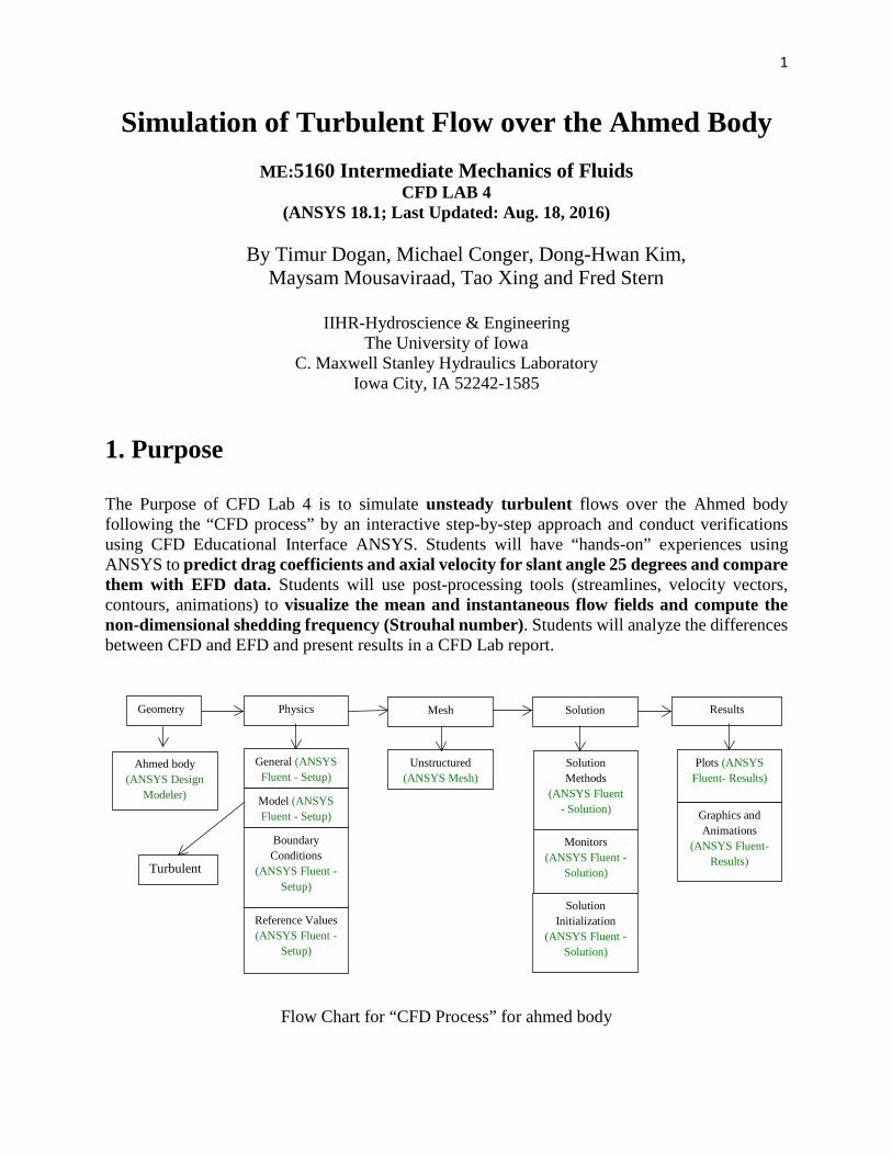
Iowa City, IA 52242-1585 1. Purpose The Purpose of CFD Lab 4 is to simulate unsteady turbulent flows over the Ahmed body following the “CFD process” by an interactive step-by-step approach and conduct verifications using CFD Educational Interface ANSYS. Students will have “hands-on” experiences using ANSYS to predict drag coefficients and axial velocity for slant angle 25 degrees and compare them with EFD data. Students will use post-processing tools (streamlines, velocity vectors, contours, animations) to visualize the mean and instantaneous flow fields and compute the non-dimensional shedding frequency (Strouhal number). Students will analyze the differences between CFD and EFD and present results in a CFD Lab report.

Flow Chart for “CFD Process” for ahmed body

Geometry Physics Mesh Solution Results

Ahmed body (ANSYS Design

Modeler)

Unstructured (ANSYS Mesh)

General (ANSYS Fluent - Setup) Model (ANSYS Fluent - Setup)

Boundary Conditions

(ANSYS Fluent -Setup)

Reference Values (ANSYS Fluent -

Setup)

Turbulent

Solution Methods

(ANSYS Fluent - Solution)

Monitors (ANSYS Fluent -

Solution)

Plots (ANSYS Fluent- Results)

Graphics and Animations

(ANSYS Fluent- Results)

Solution Initialization

(ANSYS Fluent -Solution)

2

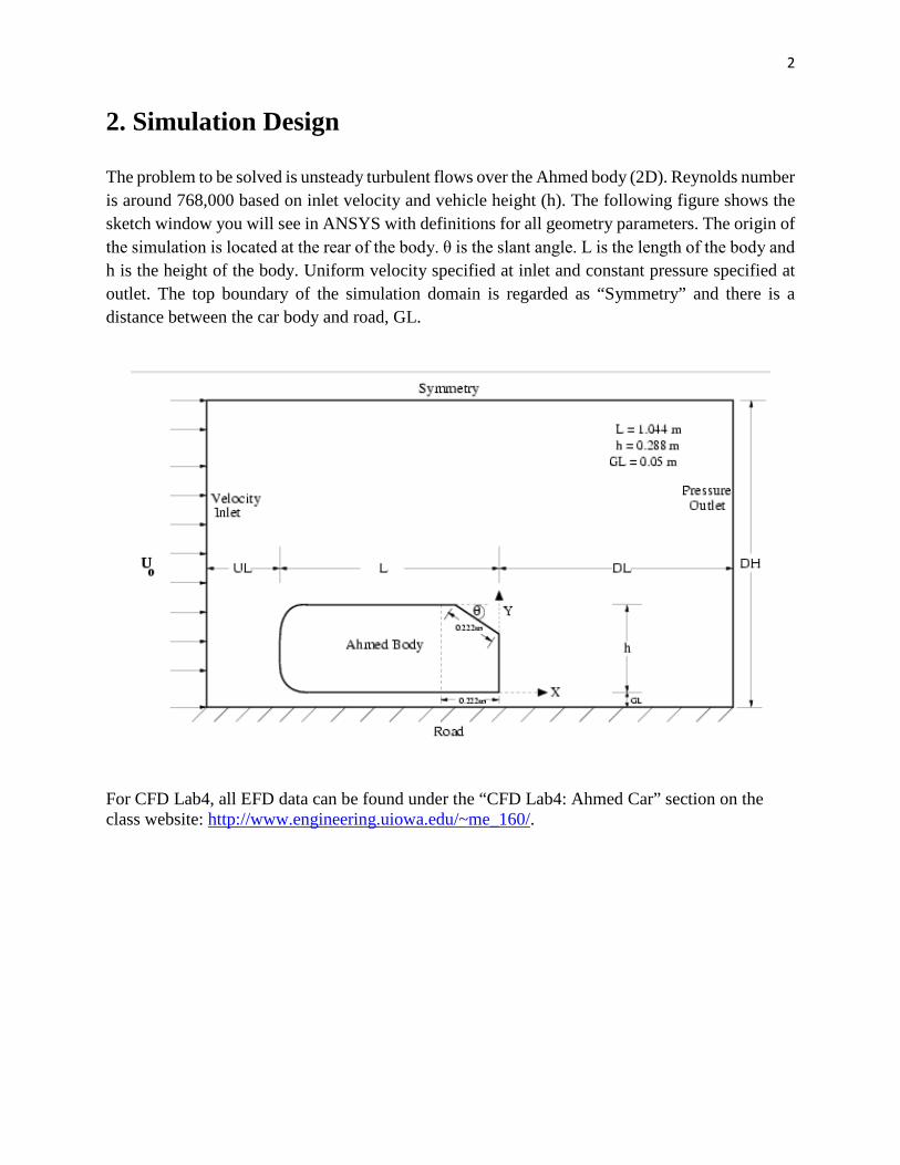
2. Simulation Design The problem to be solved is unsteady turbulent flows over the Ahmed body (2D). Reynolds number is around 768,000 based on inlet velocity and vehicle height (h). The following figure shows the sketch window you will see in ANSYS with definitions for all geometry parameters. The origin of the simulation is located at the rear of the body. θ is the slant angle. L is the length of the body and h is the height of the body. Uniform velocity specified at inlet and constant pressure specified at outlet. The top boundary of the simulation domain is regarded as “Symmetry” and there is a distance between the car body and road, GL.

For CFD Lab4, all EFD data can be found under the “CFD Lab4: Ahmed Car” section on the class website: http://www.engineering.uiowa.edu/~me_160/.

3

3. Opening ANSYS Workbench Software

3.1. Start > All Programs > ANSYS 18.1 > Workbench 18.1

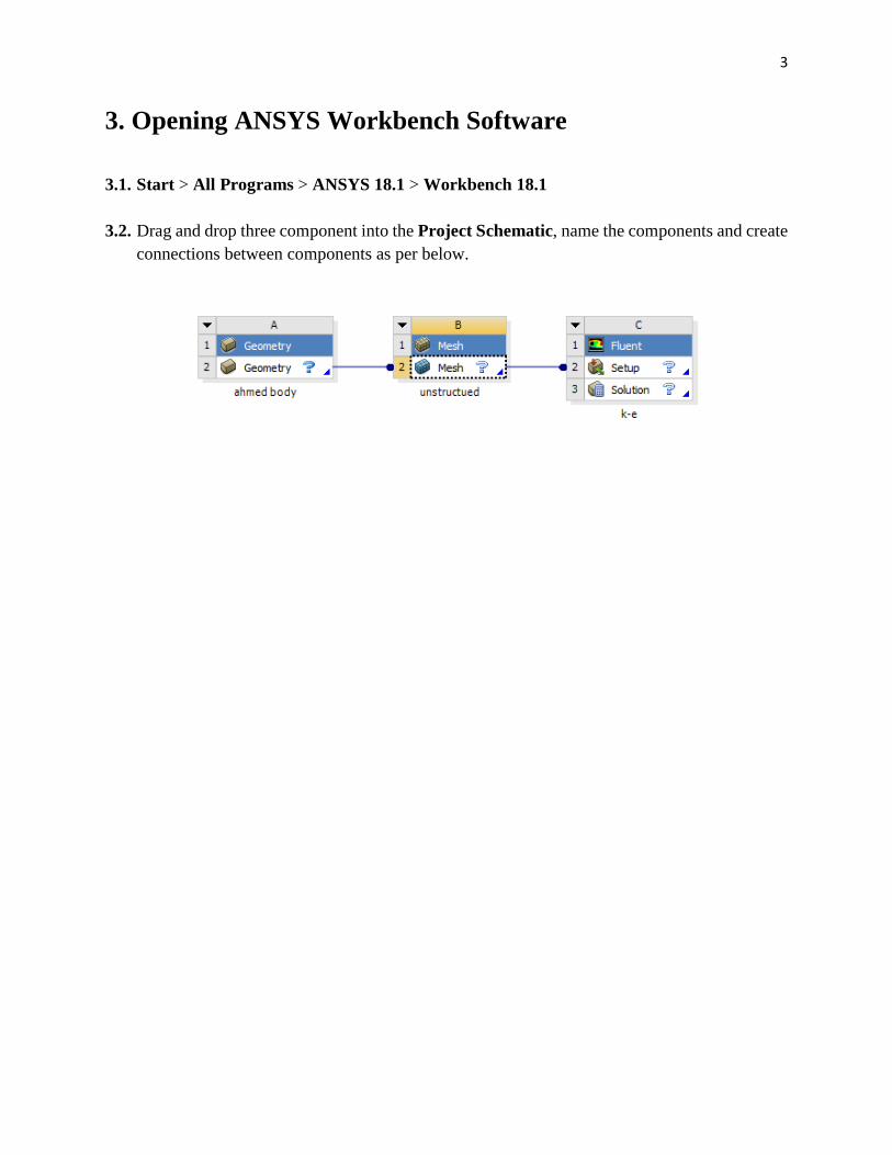
3.2. Drag and drop three component into the Project Schematic, name the components and create connections between components as per below.

4

4. Geometry Creation

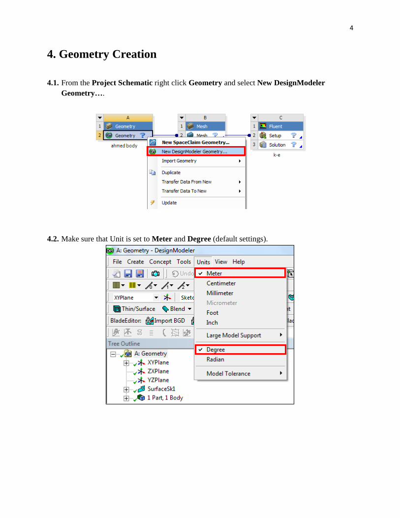
4.1. From the Project Schematic right click Geometry and select New DesignModeler Geometry….

4.2. Make sure that Unit is set to Meter and Degree (default settings).

5

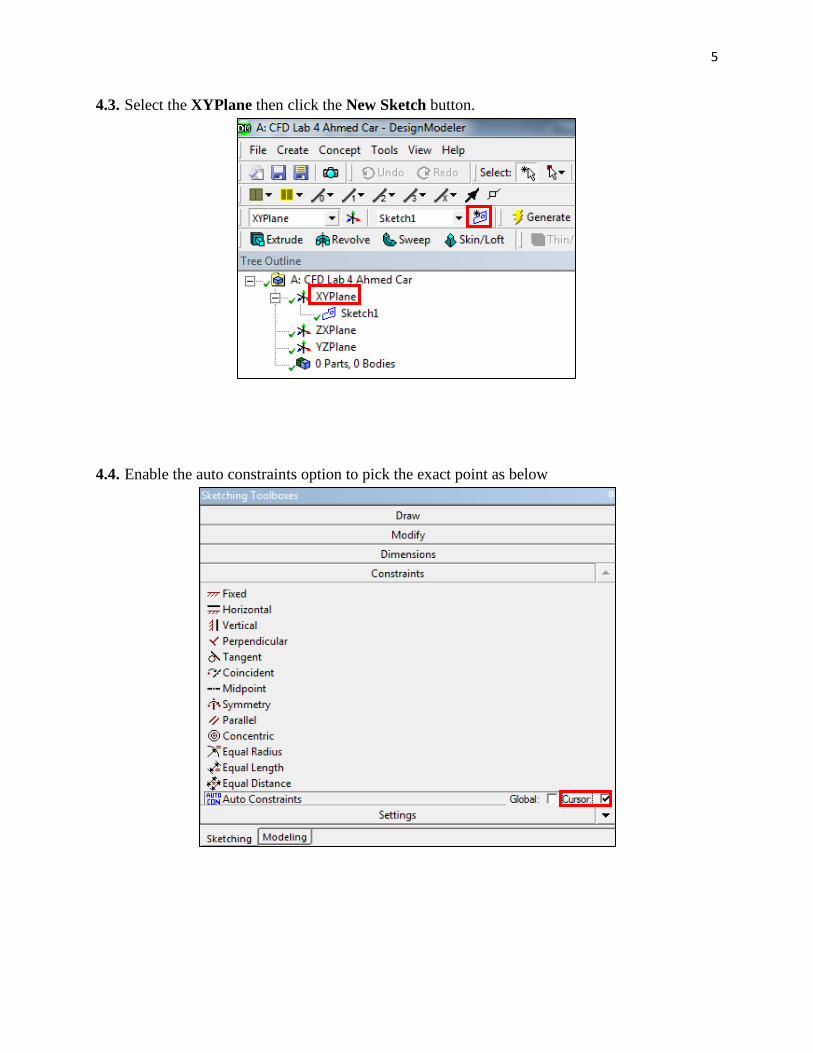
4.3. Select the XYPlane then click the New Sketch button.

4.4. Enable the auto constraints option to pick the exact point as below

6

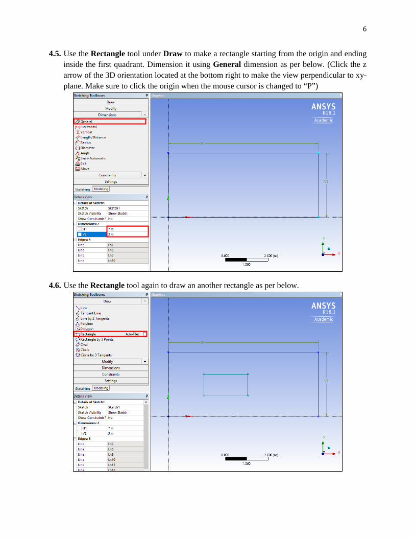
4.5. Use the Rectangle tool under Draw to make a rectangle starting from the origin and ending inside the first quadrant. Dimension it using General dimension as per below. (Click the z arrow of the 3D orientation located at the bottom right to make the view perpendicular to xy-plane. Make sure to click the origin when the mouse cursor is changed to “P”)

4.6. Use the Rectangle tool again to draw an another rectangle as per below.

7

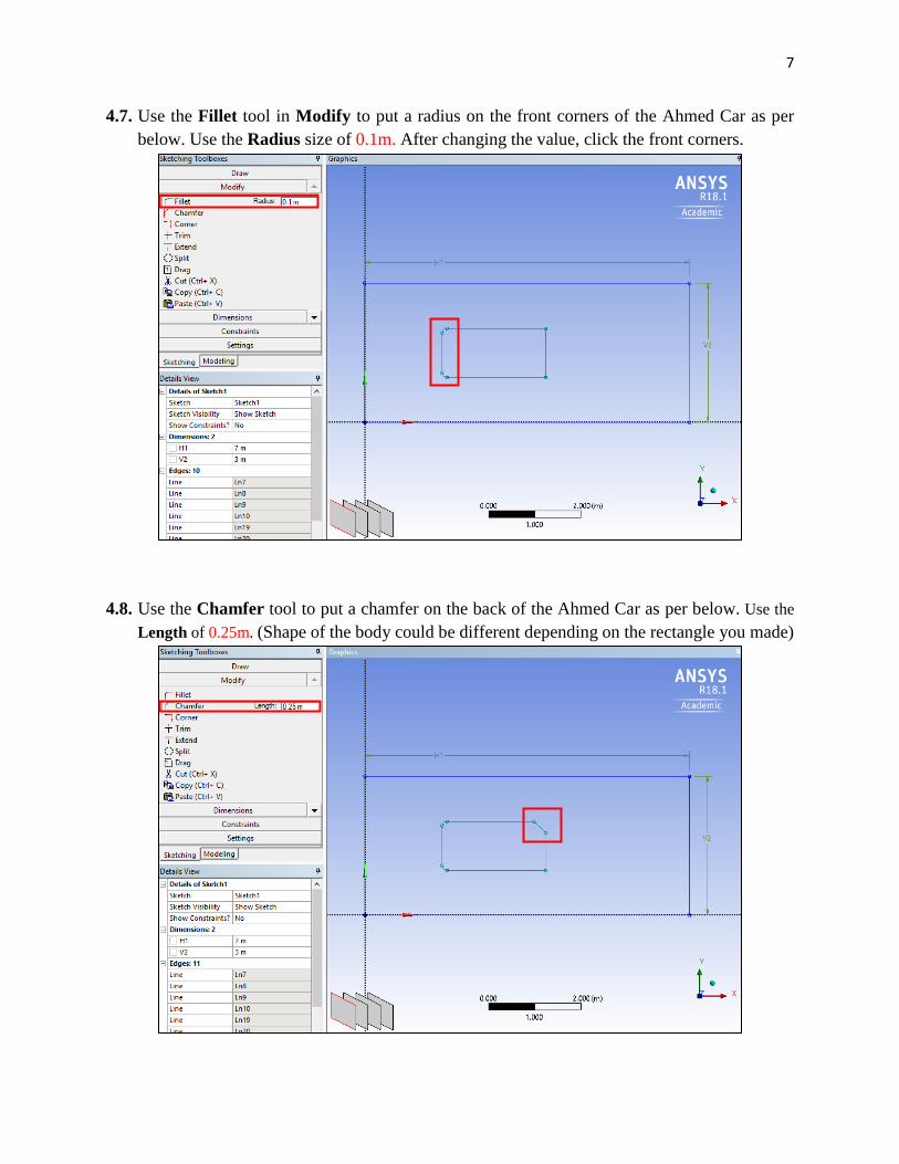
4.7. Use the Fillet tool in Modify to put a radius on the front corners of the Ahmed Car as per below. Use the Radius size of 0.1m. After changing the value, click the front corners.

4.8. Use the Chamfer tool to put a chamfer on the back of the Ahmed Car as per below. Use the Length of 0.25m. (Shape of the body could be different depending on the rectangle you made)

8

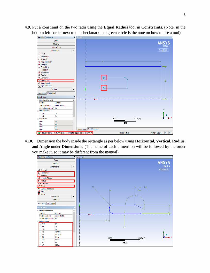
4.9. Put a constraint on the two radii using the Equal Radius tool in Constraints. (Note: in the bottom left corner next to the checkmark in a green circle is the note on how to use a tool)

4.10. Dimension the body inside the rectangle as per below using Horizontal, Vertical, Radius, and Angle under Dimensions. (The name of each dimension will be followed by the order you make it, so it may be different from the manual)

9

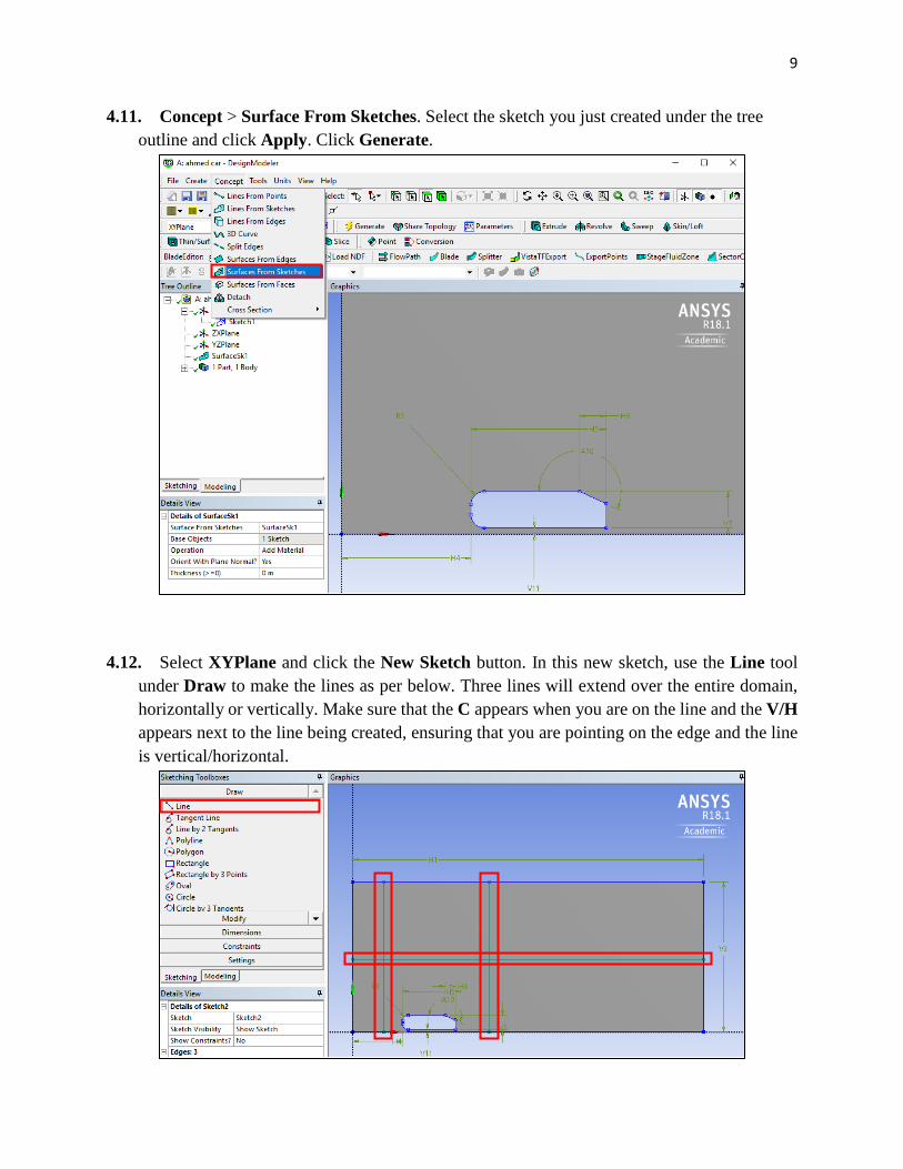
4.11. Concept > Surface From Sketches. Select the sketch you just created under the tree outline and click Apply. Click Generate.

4.12. Select XYPlane and click the New Sketch button. In this new sketch, use the Line tool under Draw to make the lines as per below. Three lines will extend over the entire domain, horizontally or vertically. Make sure that the C appears when you are on the line and the V/H appears next to the line being created, ensuring that you are pointing on the edge and the line is vertical/horizontal.

10

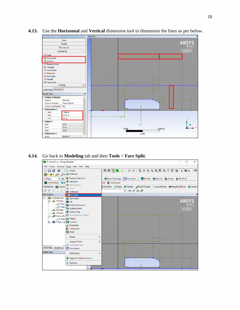
4.13. Use the Horizontal and Vertical dimension tool to dimension the lines as per below.

4.14. Go back to Modeling tab and then Tools > Face Split.

11

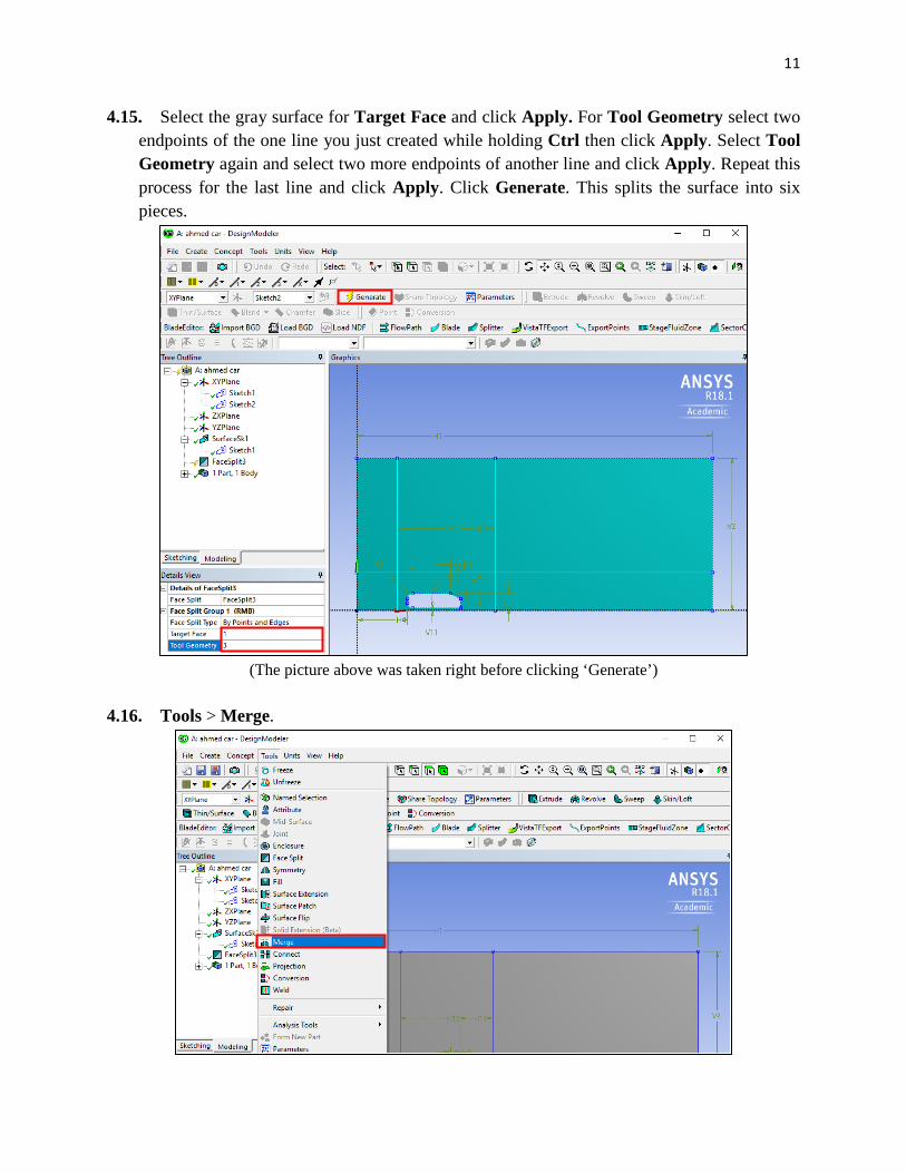
4.15. Select the gray surface for Target Face and click Apply. For Tool Geometry select two endpoints of the one line you just created while holding Ctrl then click Apply. Select Tool Geometry again and select two more endpoints of another line and click Apply. Repeat this process for the last line and click Apply. Click Generate. This splits the surface into six pieces.

(The picture above was taken right before clicking ‘Generate’)

4.16. Tools > Merge.

12

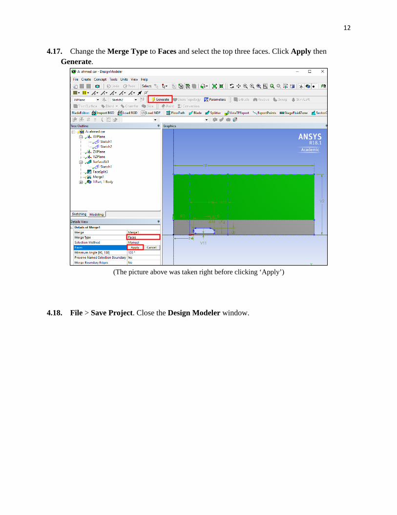
4.17. Change the Merge Type to Faces and select the top three faces. Click Apply then Generate.

(The picture above was taken right before clicking ‘Apply’)

4.18. File > Save Project. Close the Design Modeler window.

13

5. Mesh

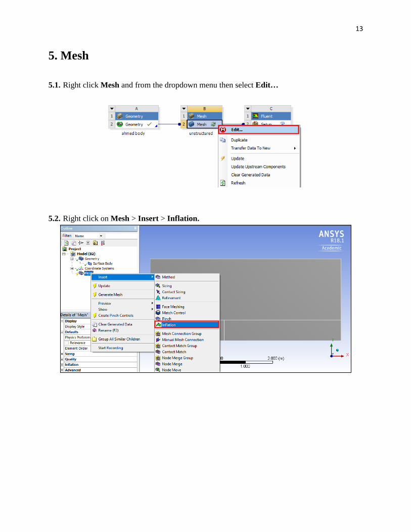
5.1. Right click Mesh and from the dropdown menu then select Edit…

5.2. Right click on Mesh > Insert > Inflation.

14

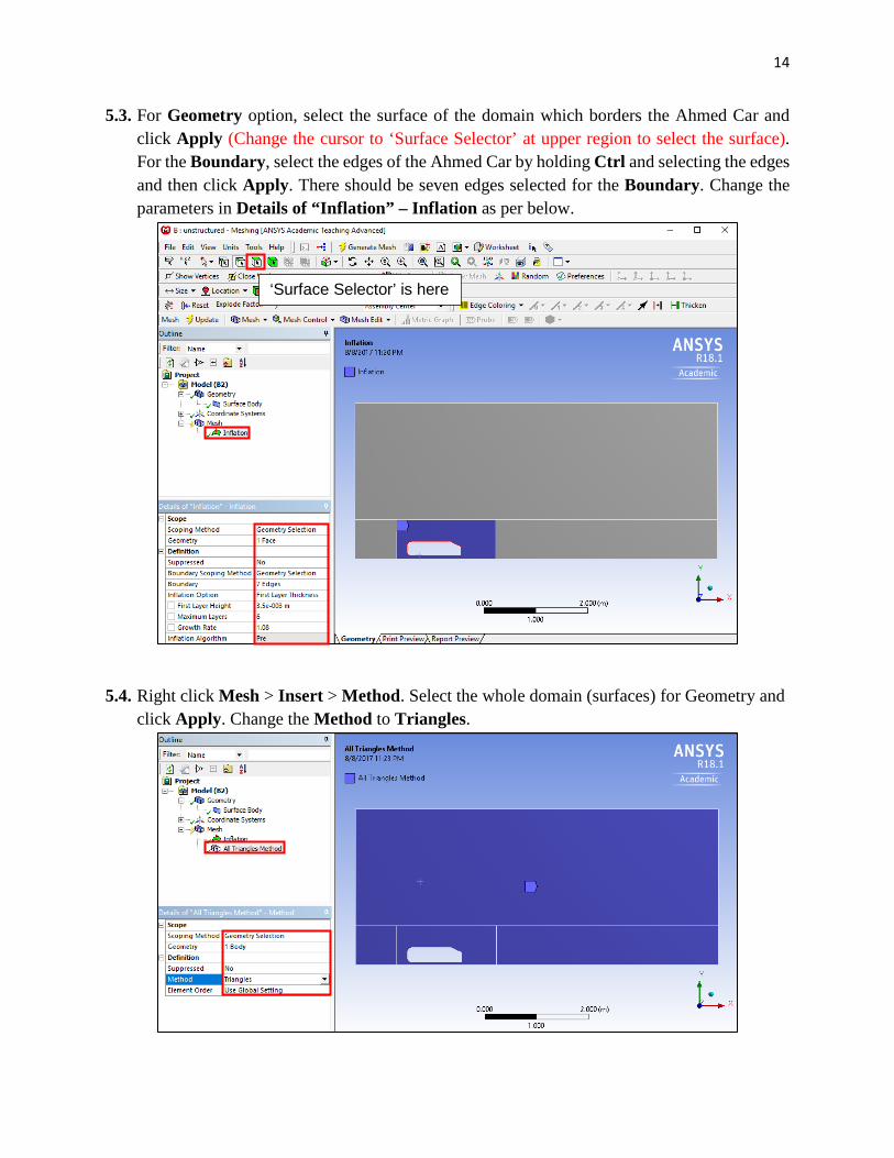
5.3. For Geometry option, select the surface of the domain which borders the Ahmed Car and click Apply (Change the cursor to ‘Surface Selector’ at upper region to select the surface). For the Boundary, select the edges of the Ahmed Car by holding Ctrl and selecting the edges and then click Apply. There should be seven edges selected for the Boundary. Change the parameters in Details of “Inflation” – Inflation as per below.

5.4. Right click Mesh > Insert > Method. Select the whole domain (surfaces) for Geometry and

click Apply. Change the Method to Triangles.

‘Surface Selector’ is here

15

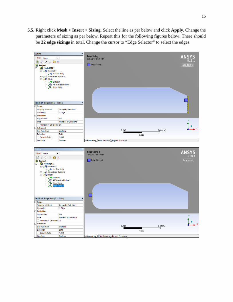
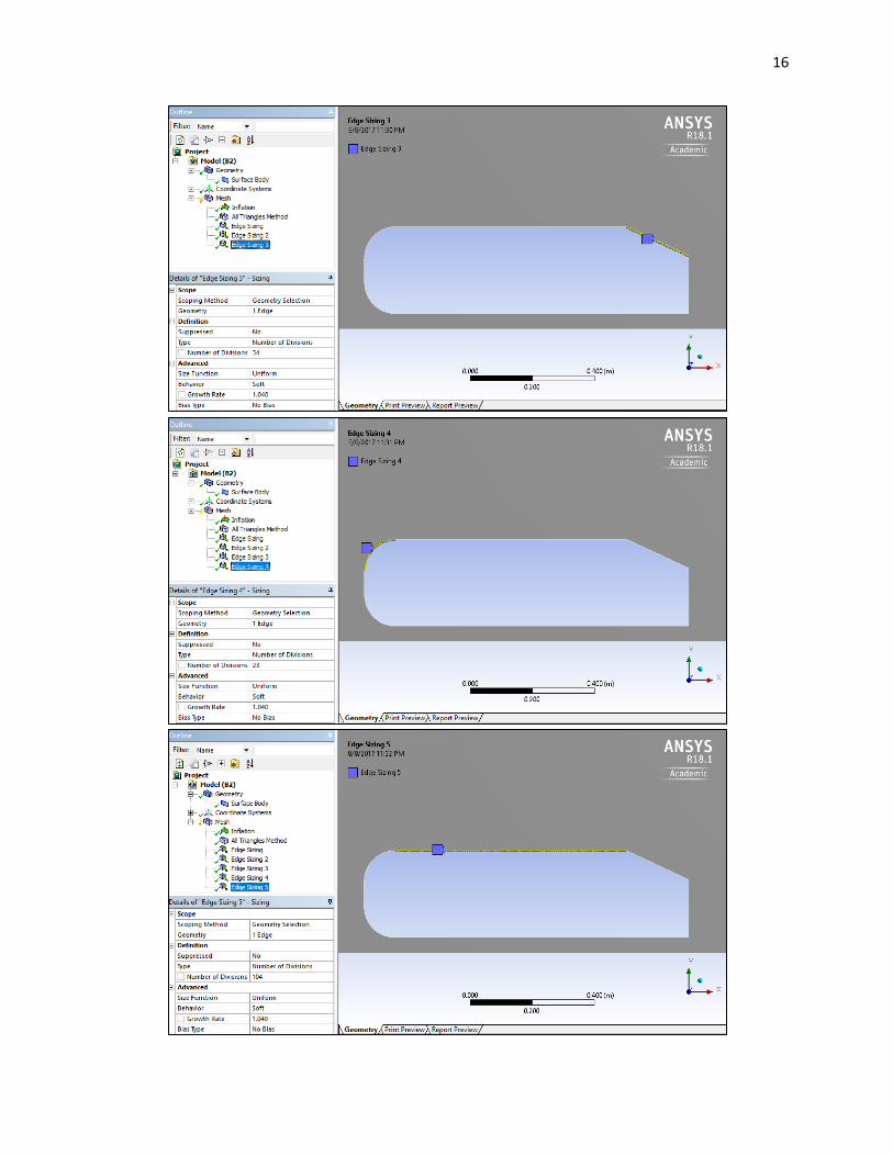
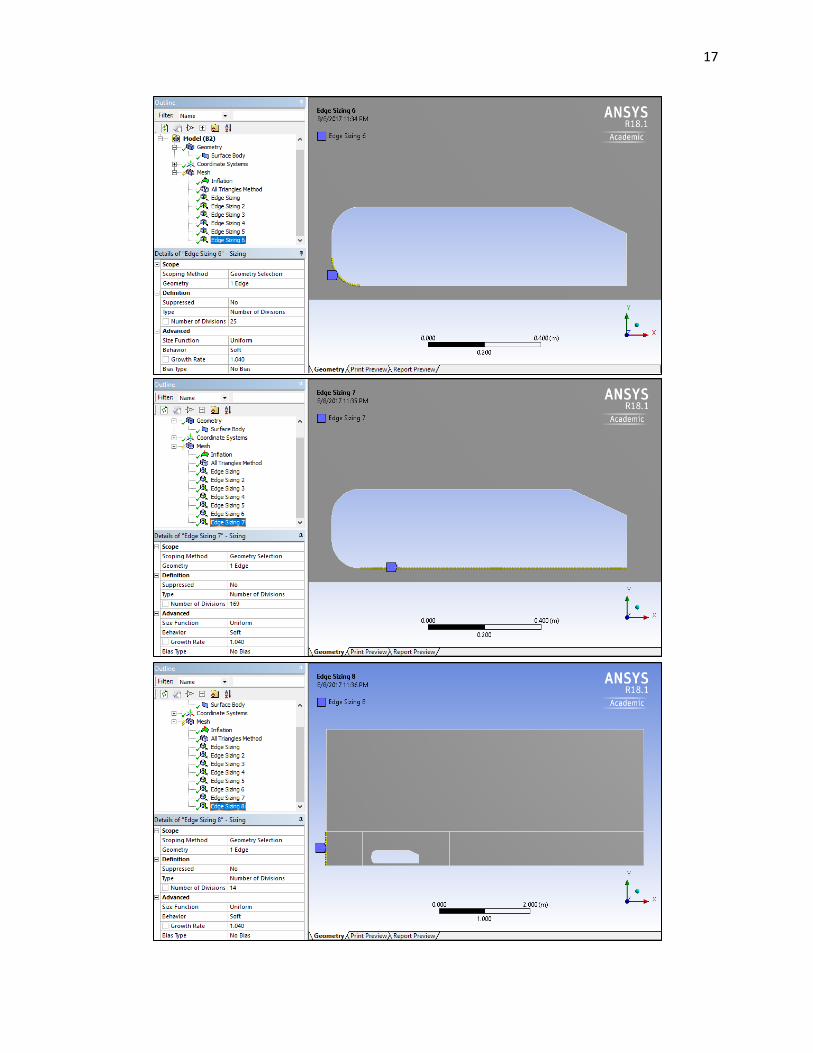
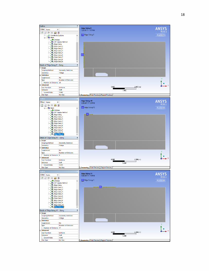
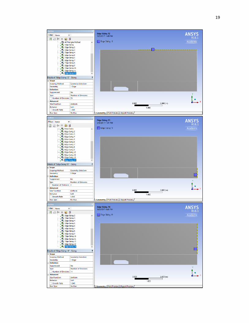
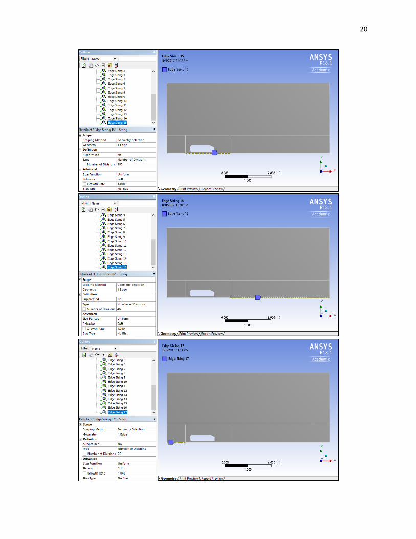
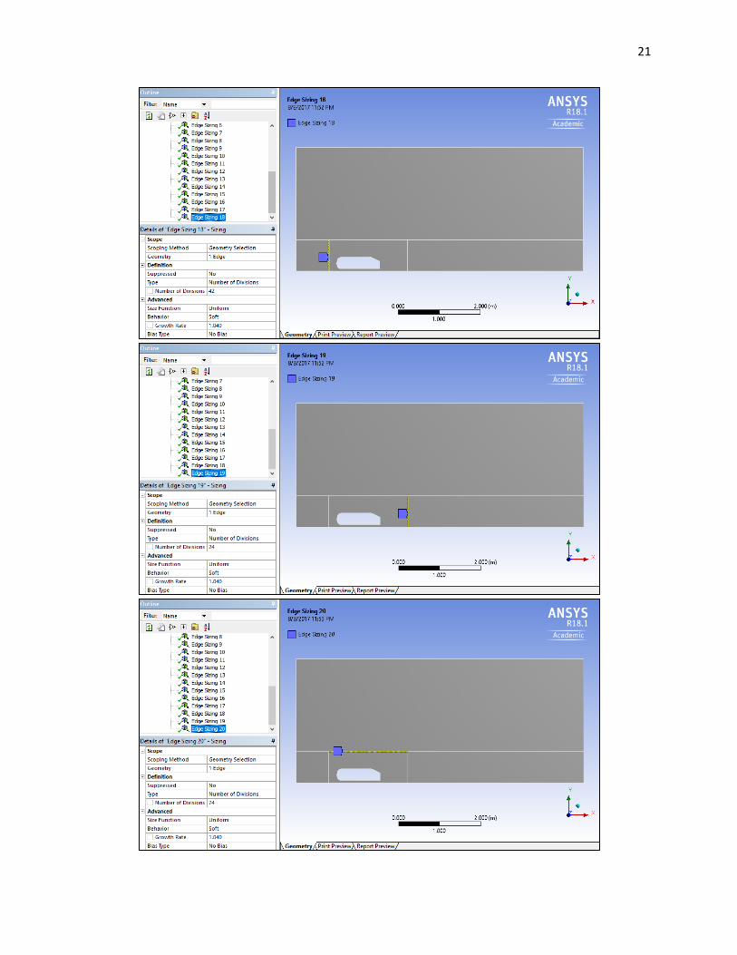
5.5. Right click Mesh > Insert > Sizing. Select the line as per below and click Apply. Change the parameters of sizing as per below. Repeat this for the following figures below. There should be 22 edge sizings in total. Change the cursor to “Edge Selector” to select the edges.

16

17

18

19

20

21

22

23

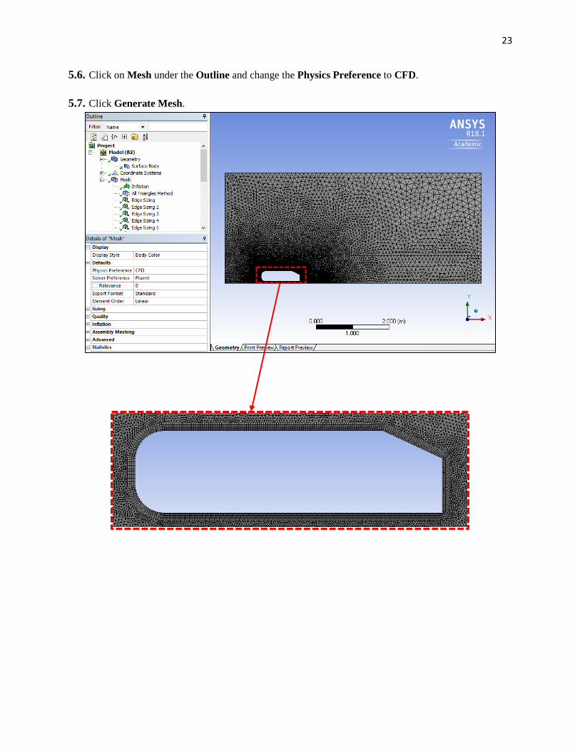
5.6. Click on Mesh under the Outline and change the Physics Preference to CFD.

5.7. Click Generate Mesh.

24

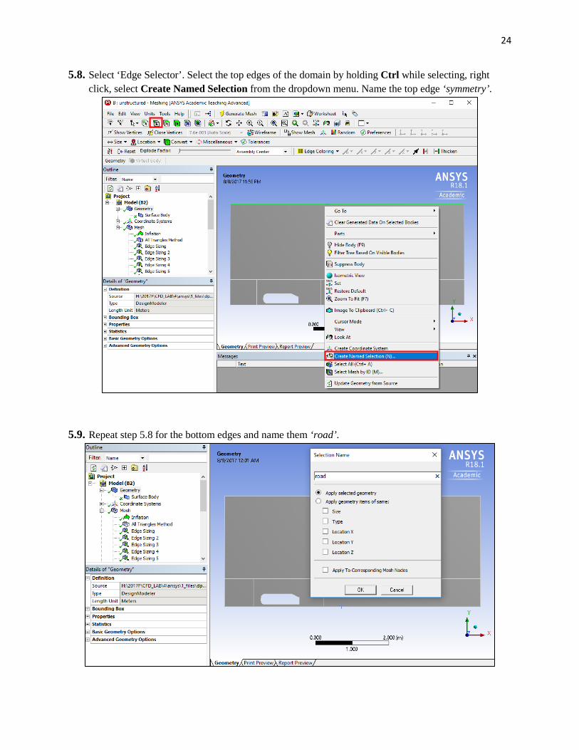
5.8. Select ‘Edge Selector’. Select the top edges of the domain by holding Ctrl while selecting, right click, select Create Named Selection from the dropdown menu. Name the top edge ‘symmetry’.

5.9. Repeat step 5.8 for the bottom edges and name them ‘road’.

25

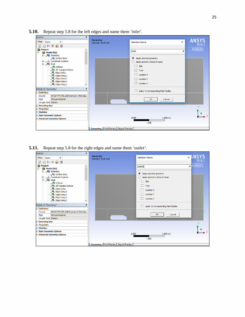
5.10. Repeat step 5.8 for the left edges and name them ‘inlet’.

5.11. Repeat step 5.8 for the right edges and name them ‘outlet’.

26

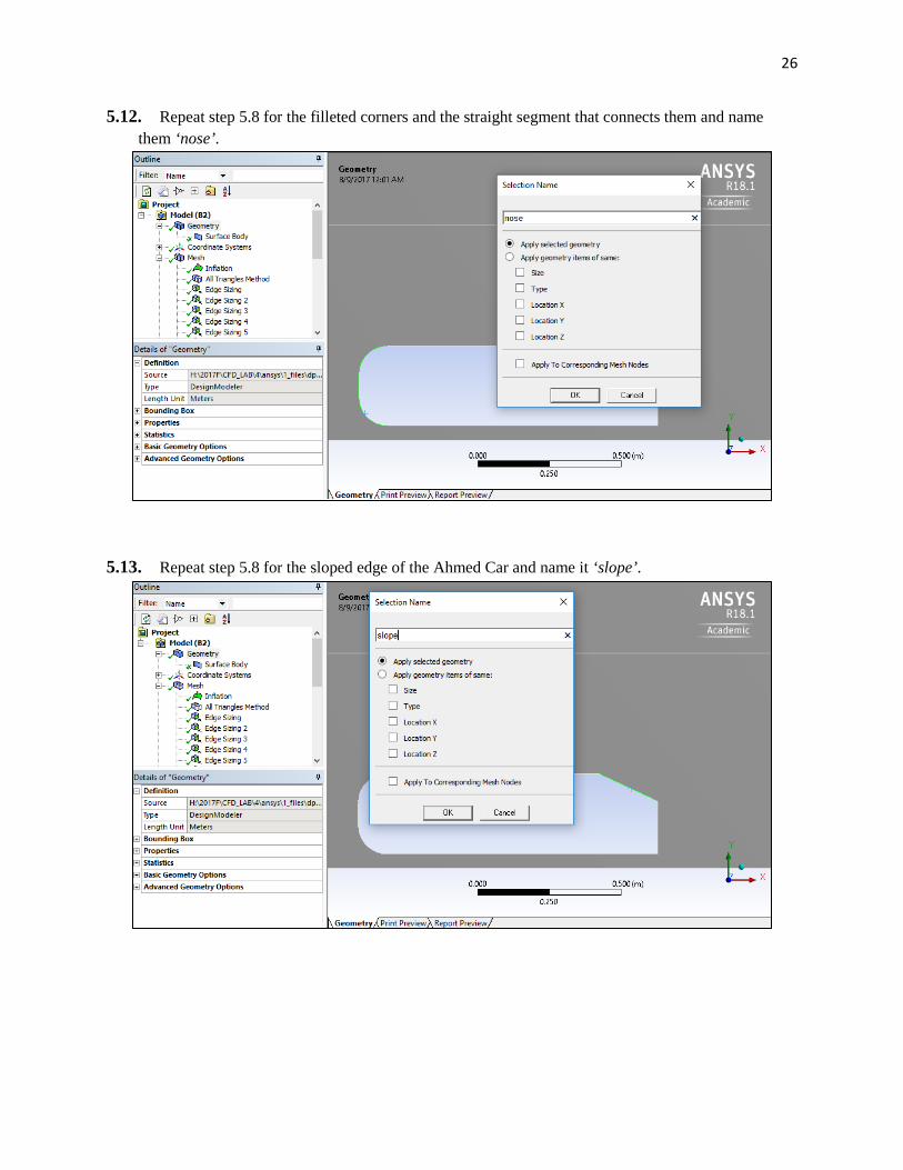
5.12. Repeat step 5.8 for the filleted corners and the straight segment that connects them and name them ‘nose’.

5.13. Repeat step 5.8 for the sloped edge of the Ahmed Car and name it ‘slope’.

27

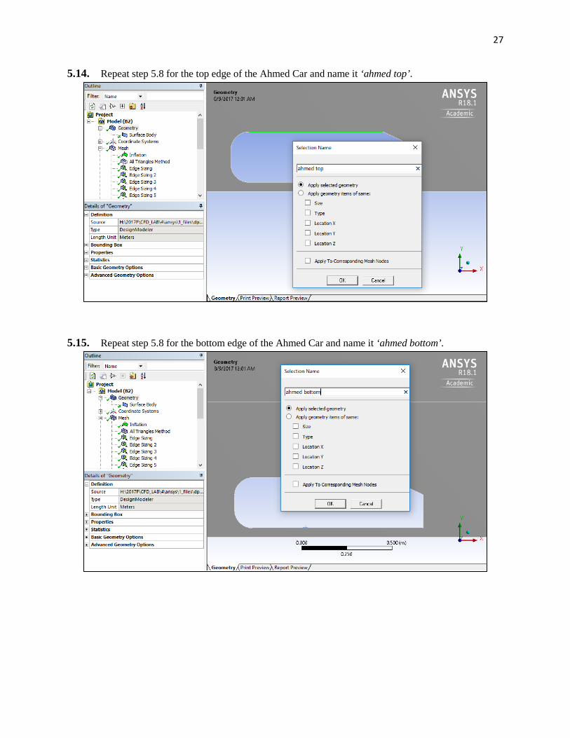
5.14. Repeat step 5.8 for the top edge of the Ahmed Car and name it ‘ahmed top’.

5.15. Repeat step 5.8 for the bottom edge of the Ahmed Car and name it ‘ahmed bottom’.

28

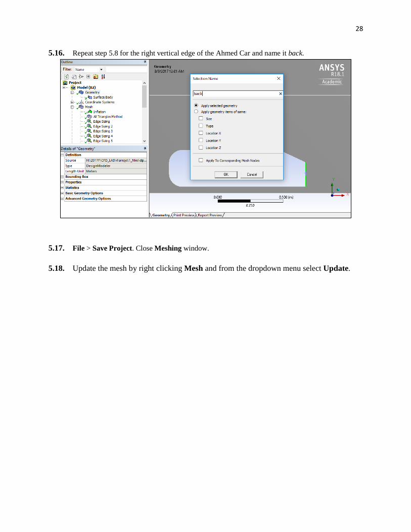
5.16. Repeat step 5.8 for the right vertical edge of the Ahmed Car and name it back.

5.17. File > Save Project. Close Meshing window.

5.18. Update the mesh by right clicking Mesh and from the dropdown menu select Update.

29

6. Setup

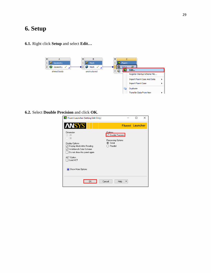
6.1. Right click Setup and select Edit…

6.2. Select Double Precision and click OK.

30

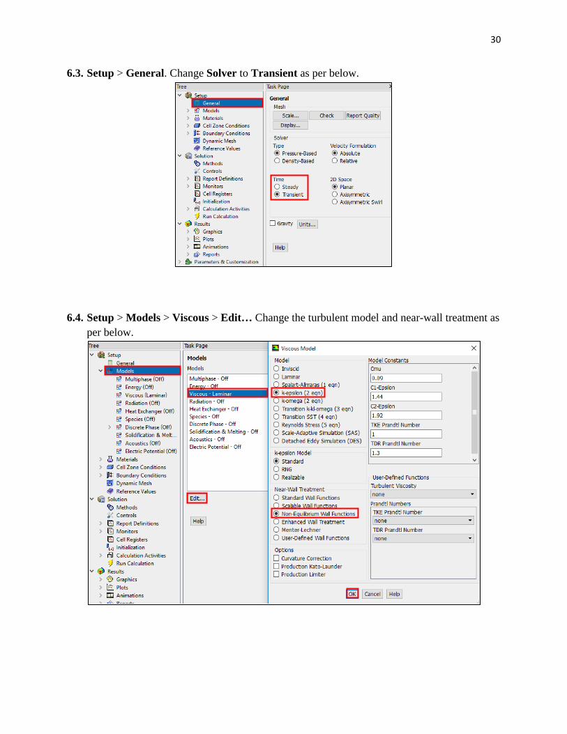
6.3. Setup > General. Change Solver to Transient as per below.

6.4. Setup > Models > Viscous > Edit… Change the turbulent model and near-wall treatment as per below.

31

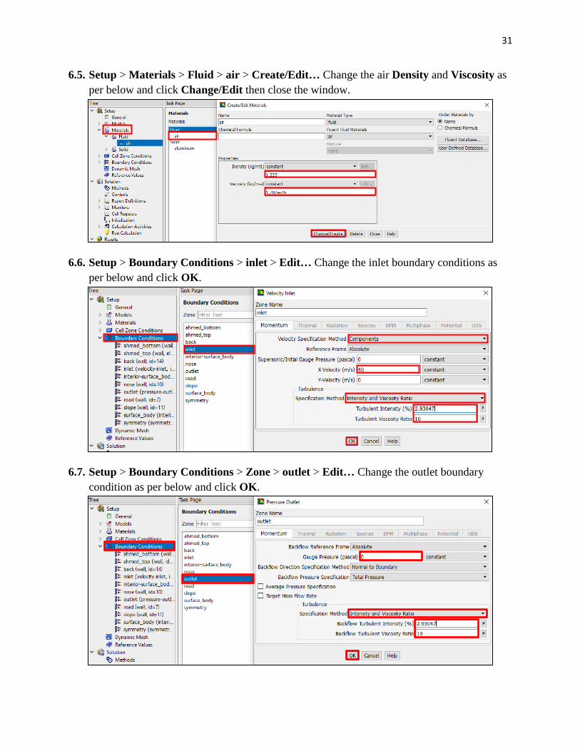
6.5. Setup > Materials > Fluid > air > Create/Edit… Change the air Density and Viscosity as per below and click Change/Edit then close the window.

6.6. Setup > Boundary Conditions > inlet > Edit… Change the inlet boundary conditions as

per below and click OK.

6.7. Setup > Boundary Conditions > Zone > outlet > Edit… Change the outlet boundary condition as per below and click OK.

32

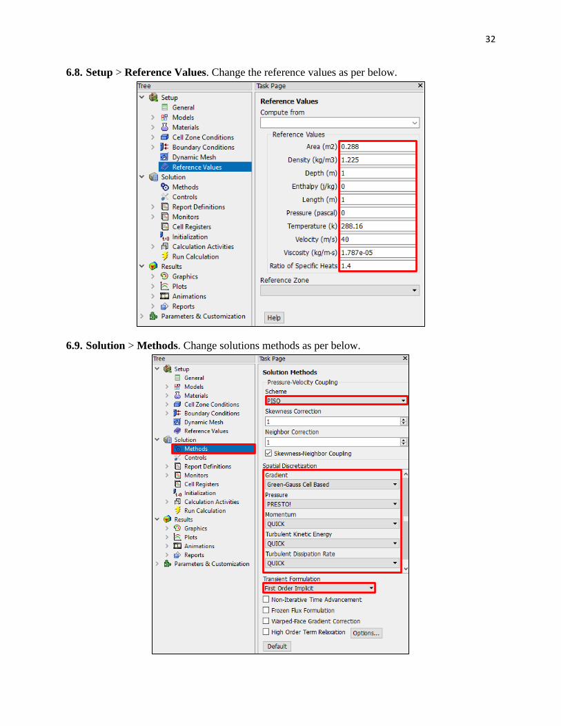
6.8. Setup > Reference Values. Change the reference values as per below.

6.9. Solution > Methods. Change solutions methods as per below.

33

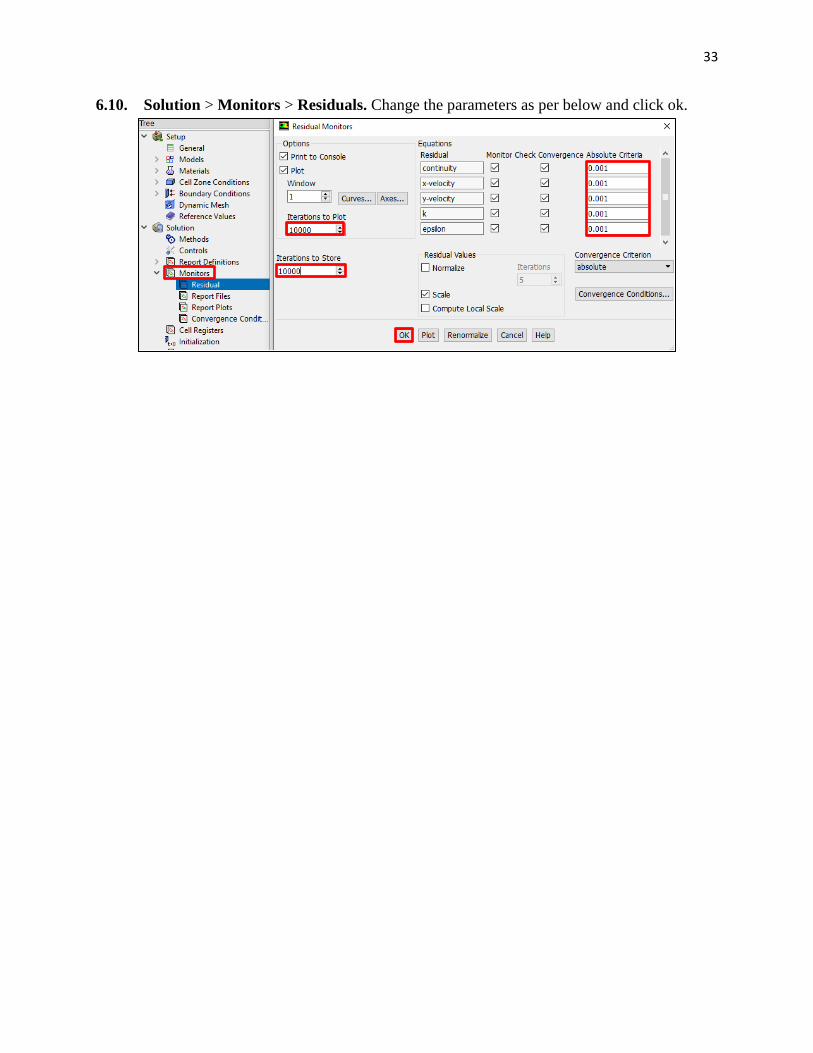
6.10. Solution > Monitors > Residuals. Change the parameters as per below and click ok.

34

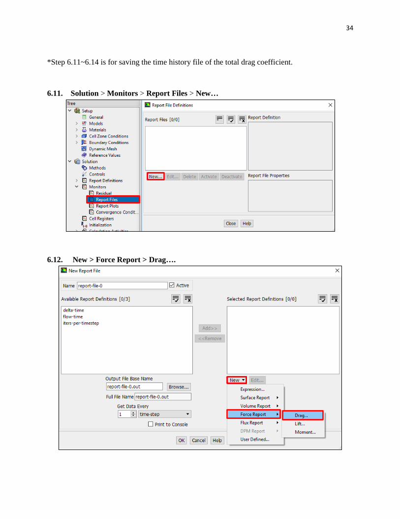
*Step 6.11~6.14 is for saving the time history file of the total drag coefficient. 6.11. Solution > Monitors > Report Files > New…

6.12. New > Force Report > Drag….

35

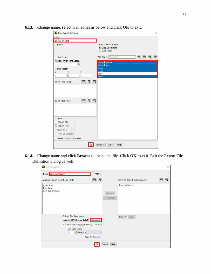
6.13. Change name, select wall zones as below and click OK to exit.

6.14. Change name and click Browse to locate the file. Click OK to exit. Exit the Report File Definition dialog as well.

36

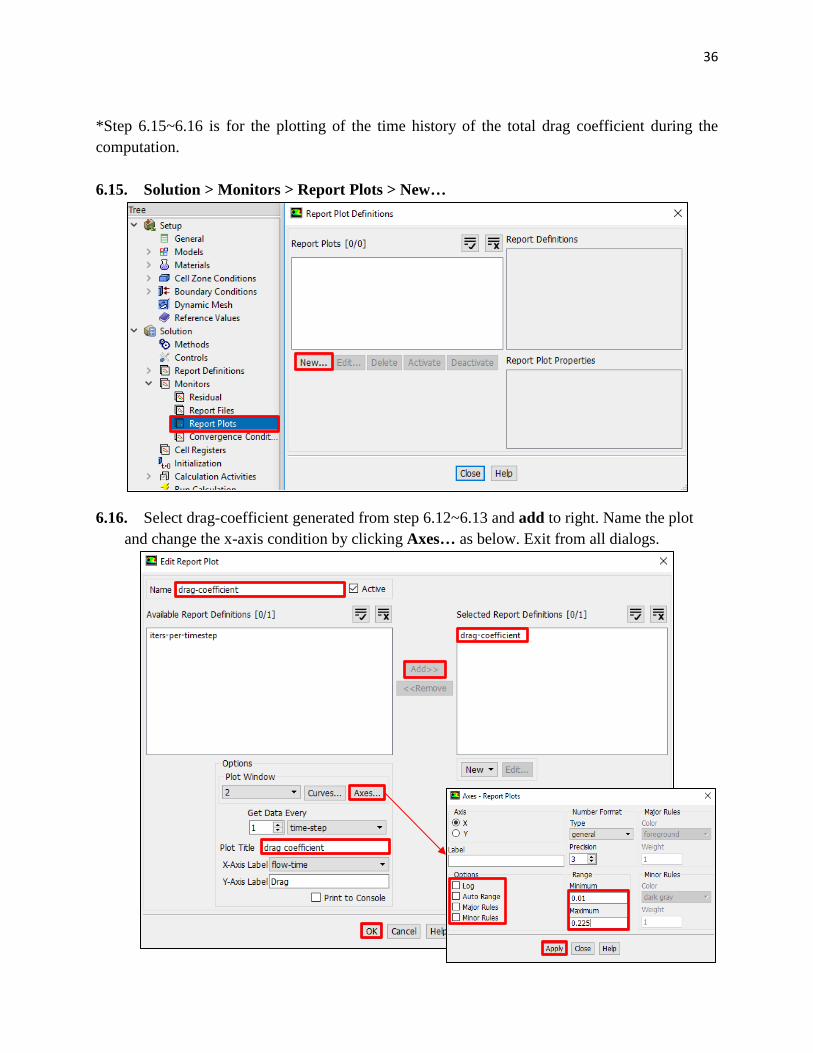
*Step 6.15~6.16 is for the plotting of the time history of the total drag coefficient during the computation.

6.15. Solution > Monitors > Report Plots > New…

6.16. Select drag-coefficient generated from step 6.12~6.13 and add to right. Name the plot and change the x-axis condition by clicking Axes… as below. Exit from all dialogs.

37

6.17. Solution > Initialization. Change X-Velocity and turbulent parameters as per below. Click Initialize.

38

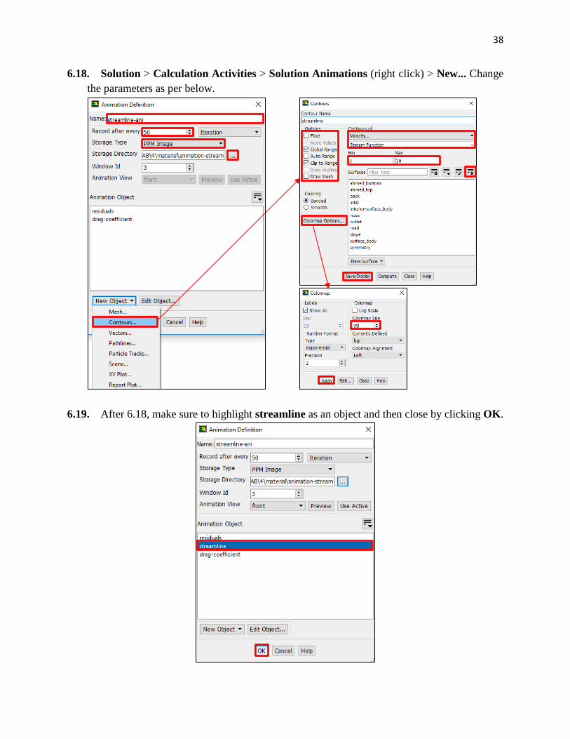
6.18. Solution > Calculation Activities > Solution Animations (right click) > New... Change the parameters as per below.

6.19. After 6.18, make sure to highlight streamline as an object and then close by clicking OK.

39

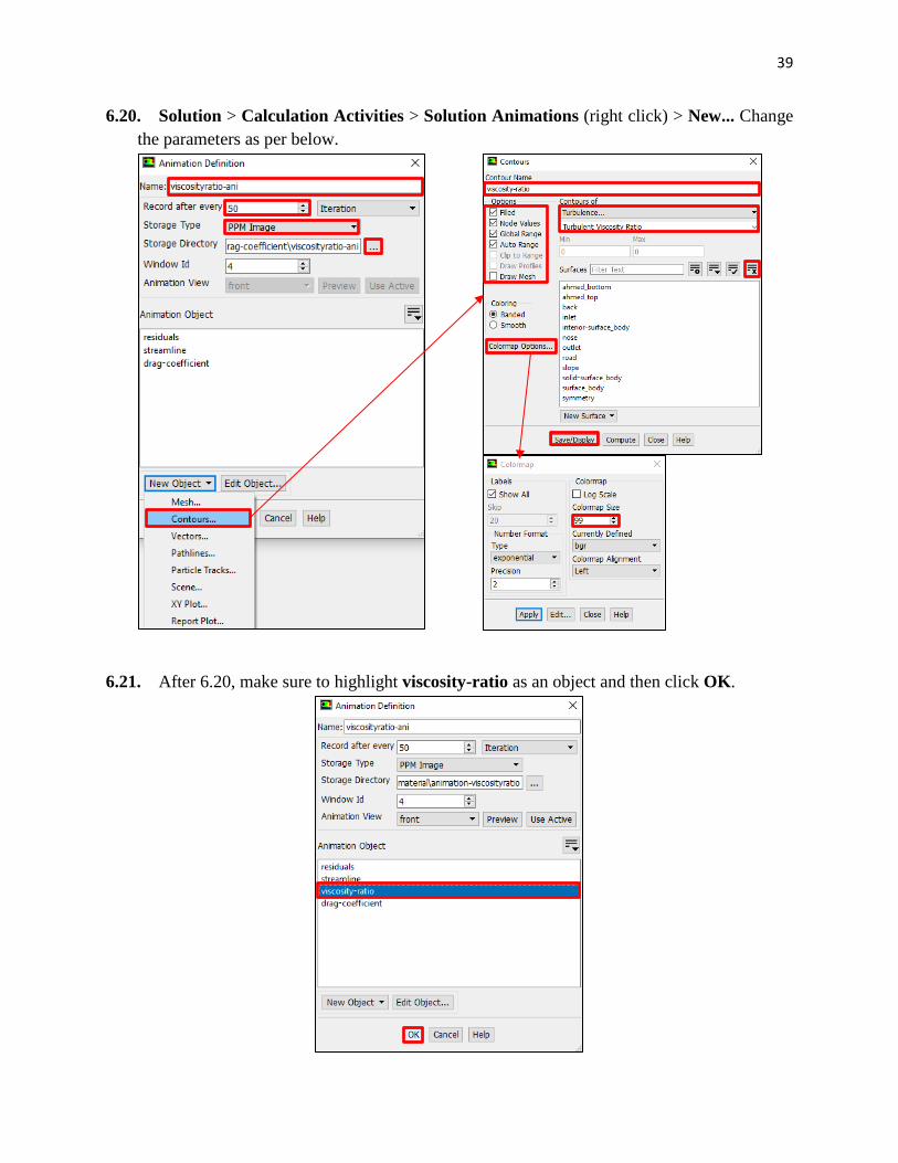
6.20. Solution > Calculation Activities > Solution Animations (right click) > New... Change the parameters as per below.

6.21. After 6.20, make sure to highlight viscosity-ratio as an object and then click OK.

40

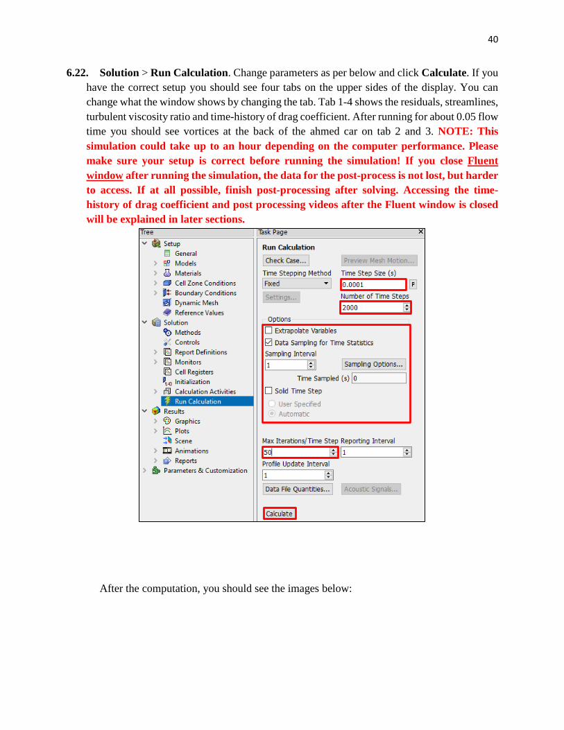
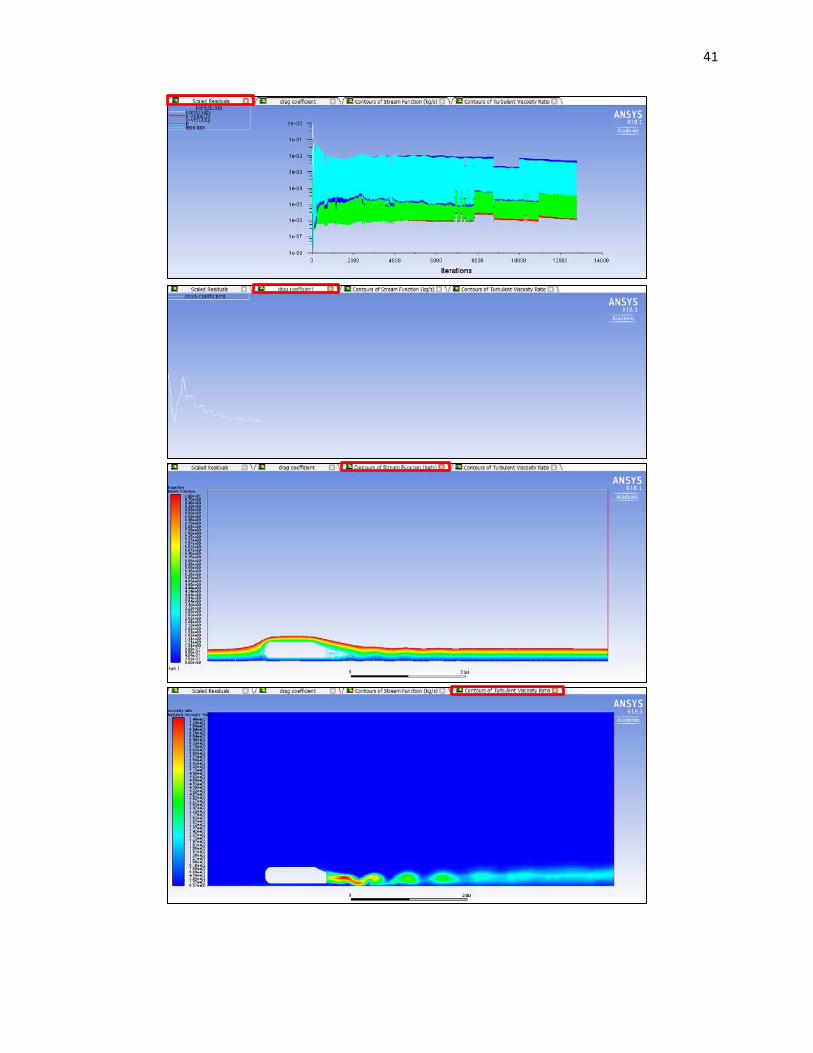
6.22. Solution > Run Calculation. Change parameters as per below and click Calculate. If you have the correct setup you should see four tabs on the upper sides of the display. You can change what the window shows by changing the tab. Tab 1-4 shows the residuals, streamlines, turbulent viscosity ratio and time-history of drag coefficient. After running for about 0.05 flow time you should see vortices at the back of the ahmed car on tab 2 and 3. NOTE: This simulation could take up to an hour depending on the computer performance. Please make sure your setup is correct before running the simulation! If you close Fluent window after running the simulation, the data for the post-process is not lost, but harder to access. If at all possible, finish post-processing after solving. Accessing the time-history of drag coefficient and post processing videos after the Fluent window is closed will be explained in later sections.

After the computation, you should see the images below:

41

42

7. Results

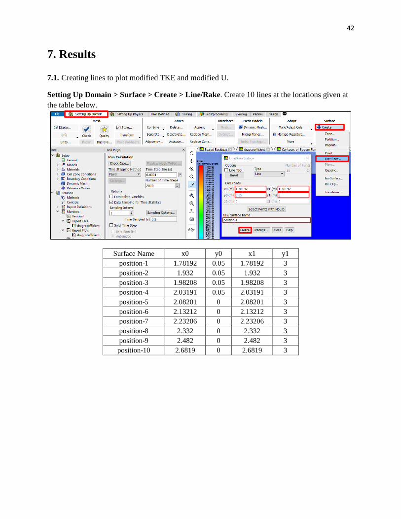
7.1. Creating lines to plot modified TKE and modified U.

Setting Up Domain > Surface > Create > Line/Rake. Create 10 lines at the locations given at the table below.

Surface Name x0 y0 x1 y1 position-1 1.78192 0.05 1.78192 3 position-2 1.932 0.05 1.932 3 position-3 1.98208 0.05 1.98208 3 position-4 2.03191 0.05 2.03191 3 position-5 2.08201 0 2.08201 3 position-6 2.13212 0 2.13212 3 position-7 2.23206 0 2.23206 3 position-8 2.332 0 2.332 3 position-9 2.482 0 2.482 3 position-10 2.6819 0 2.6819 3

43

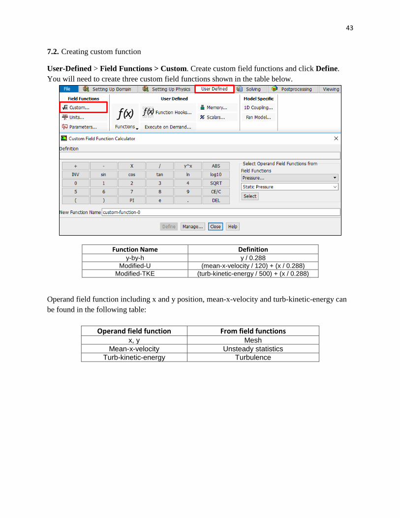
7.2. Creating custom function

User-Defined > Field Functions > Custom. Create custom field functions and click Define. You will need to create three custom field functions shown in the table below.

Function Name Definition y-by-h y / 0.288

Modified-U (mean-x-velocity / 120) + (x / 0.288) Modified-TKE (turb-kinetic-energy / 500) + (x / 0.288)

Operand field function including x and y position, mean-x-velocity and turb-kinetic-energy can be found in the following table:

Operand field function From field functions x, y Mesh

Mean-x-velocity Unsteady statistics Turb-kinetic-energy Turbulence

44

7.3. Plotting values along the lines created

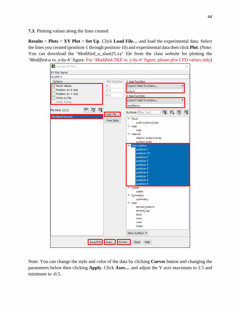
Results > Plots > XY Plot > Set Up. Click Load File… and load the experimental data. Select the lines you created (position-1 through position-10) and experimental data then click Plot. (Note: You can download the ‘Modified_u_slant25.xy’ file from the class website for plotting the ‘Modified-u vs. y-by-h’ figure. For ‘Modified-TKE vs. y-by-h’ figure, please plot CFD values only)

Note: You can change the style and color of the data by clicking Curves button and changing the parameters below then clicking Apply. Click Axes… and adjust the Y axis maximum to 2.5 and minimum to -0.5.

45

Result:

46

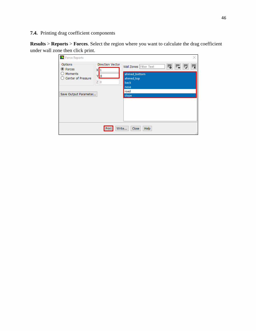
7.4. Printing drag coefficient components Results > Reports > Forces. Select the region where you want to calculate the drag coefficient under wall zone then click print.

47

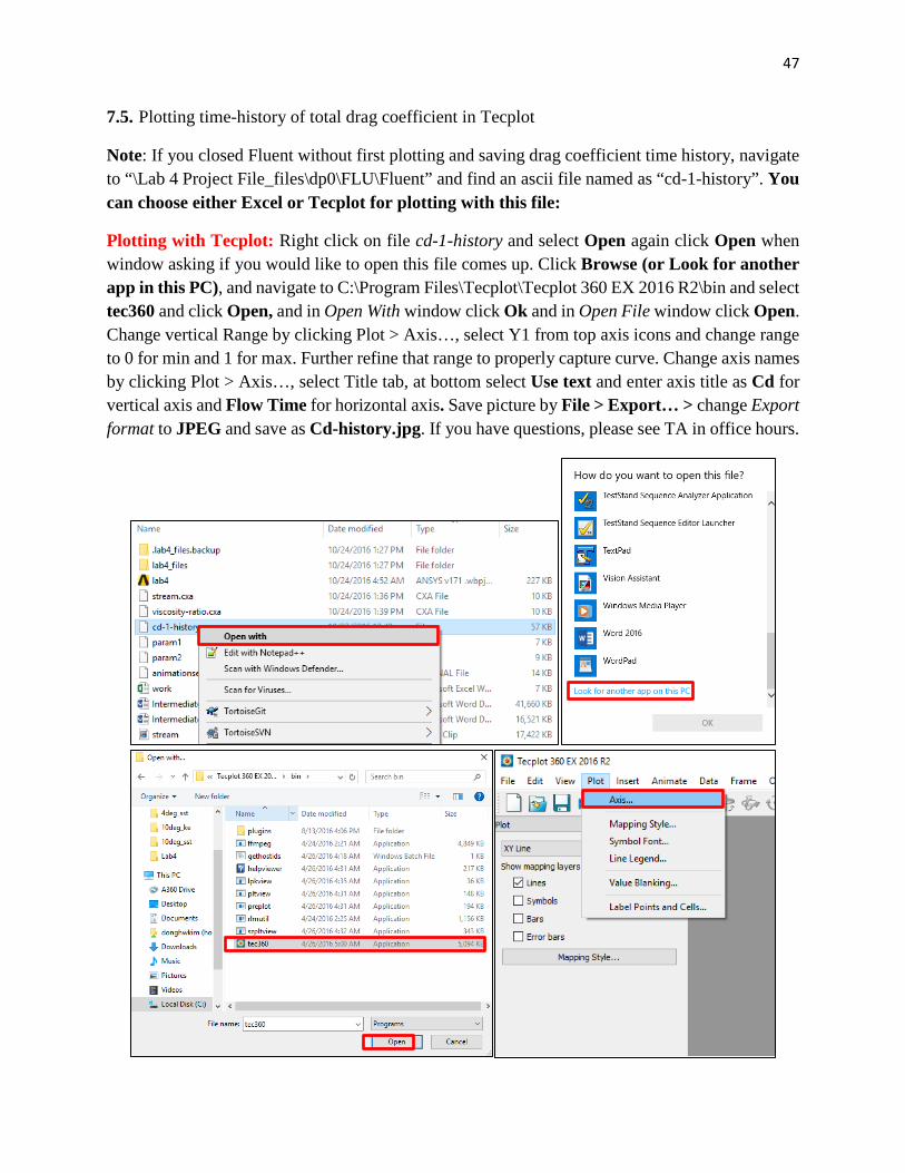
7.5. Plotting time-history of total drag coefficient in Tecplot Note: If you closed Fluent without first plotting and saving drag coefficient time history, navigate to “\Lab 4 Project File_files\dp0\FLU\Fluent” and find an ascii file named as “cd-1-history”. You can choose either Excel or Tecplot for plotting with this file:

Plotting with Tecplot: Right click on file cd-1-history and select Open again click Open when window asking if you would like to open this file comes up. Click Browse (or Look for another app in this PC), and navigate to C:\Program Files\Tecplot\Tecplot 360 EX 2016 R2\bin and select tec360 and click Open, and in Open With window click Ok and in Open File window click Open. Change vertical Range by clicking Plot > Axis…, select Y1 from top axis icons and change range to 0 for min and 1 for max. Further refine that range to properly capture curve. Change axis names by clicking Plot > Axis…, select Title tab, at bottom select Use text and enter axis title as Cd for vertical axis and Flow Time for horizontal axis. Save picture by File > Export… > change Export format to JPEG and save as Cd-history.jpg. If you have questions, please see TA in office hours.

48

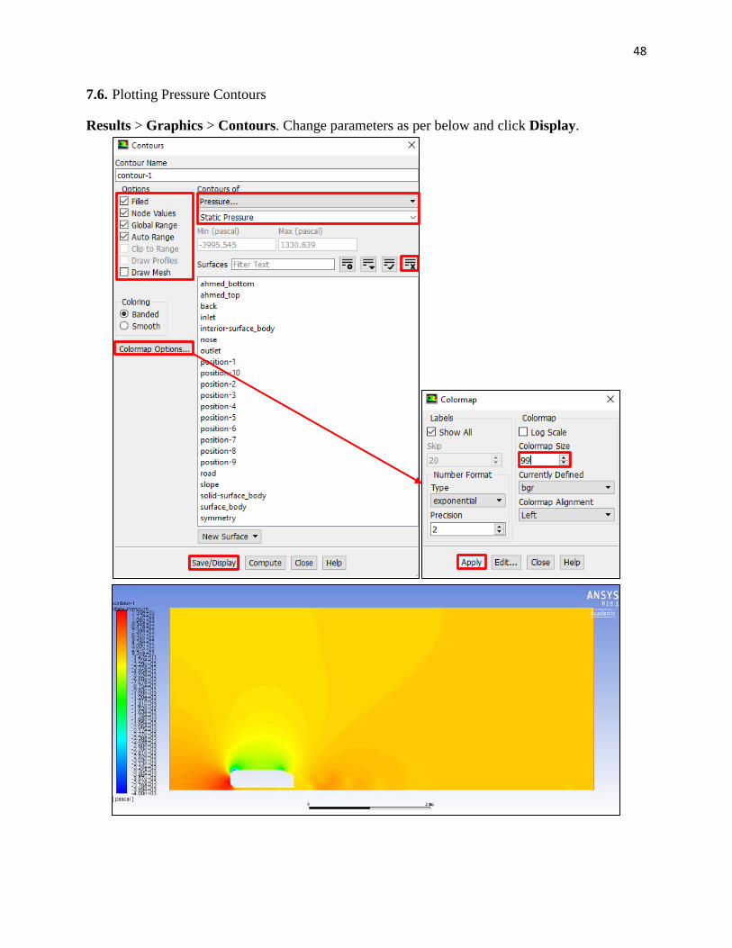
7.6. Plotting Pressure Contours Results > Graphics > Contours. Change parameters as per below and click Display.

49

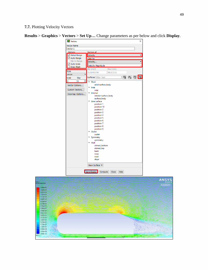
7.7. Plotting Velocity Vectors Results > Graphics > Vectors > Set Up… Change parameters as per below and click Display.

50

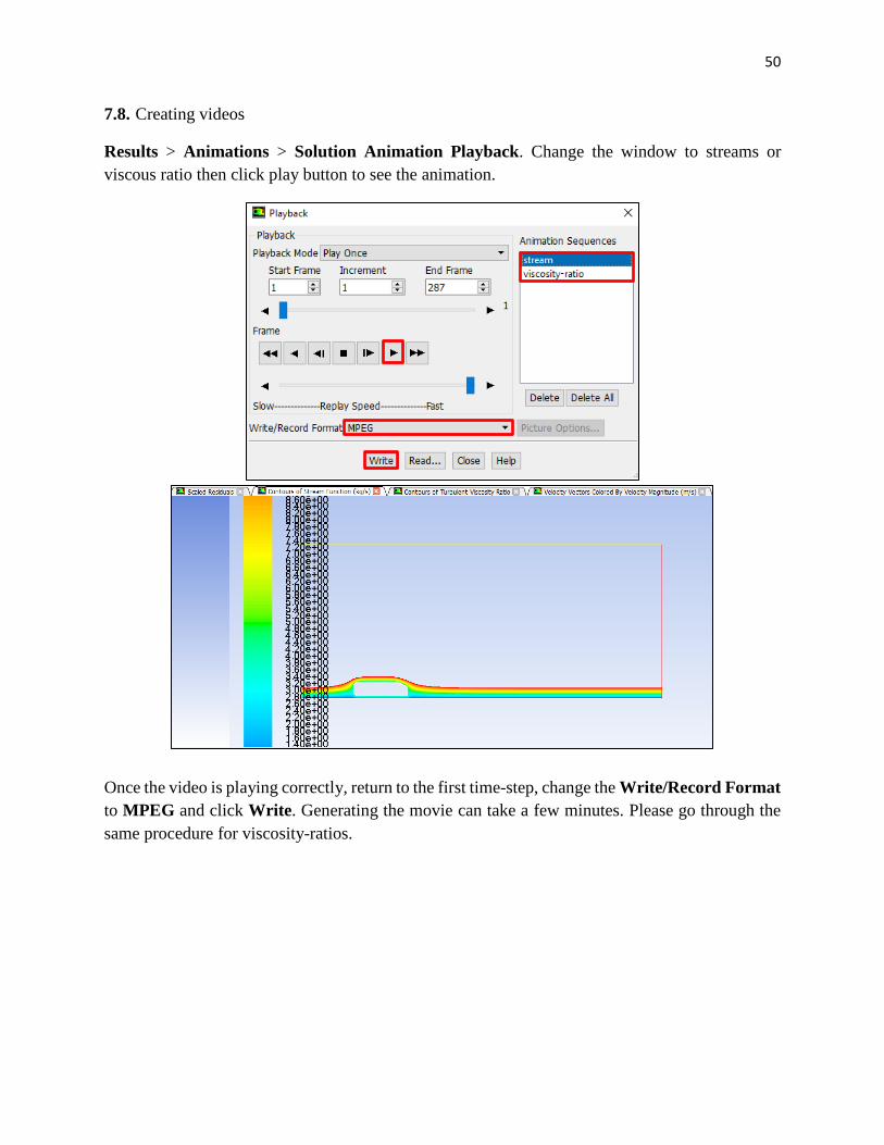
7.8. Creating videos

Results > Animations > Solution Animation Playback. Change the window to streams or viscous ratio then click play button to see the animation.

Once the video is playing correctly, return to the first time-step, change the Write/Record Format to MPEG and click Write. Generating the movie can take a few minutes. Please go through the same procedure for viscosity-ratios.

51

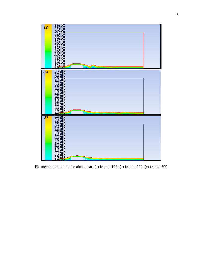
Stream

Pictures of streamline for ahmed car: (a) frame=100; (b) frame=200; (c) frame=300

(a)

(b)

(c)

52

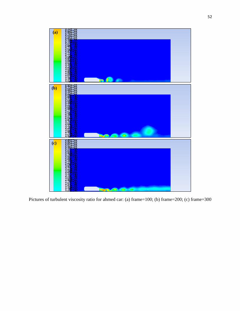
Pictures of turbulent viscosity ratio for ahmed car: (a) frame=100; (b) frame=200; (c) frame=300

(a)

(b)

(c)

53

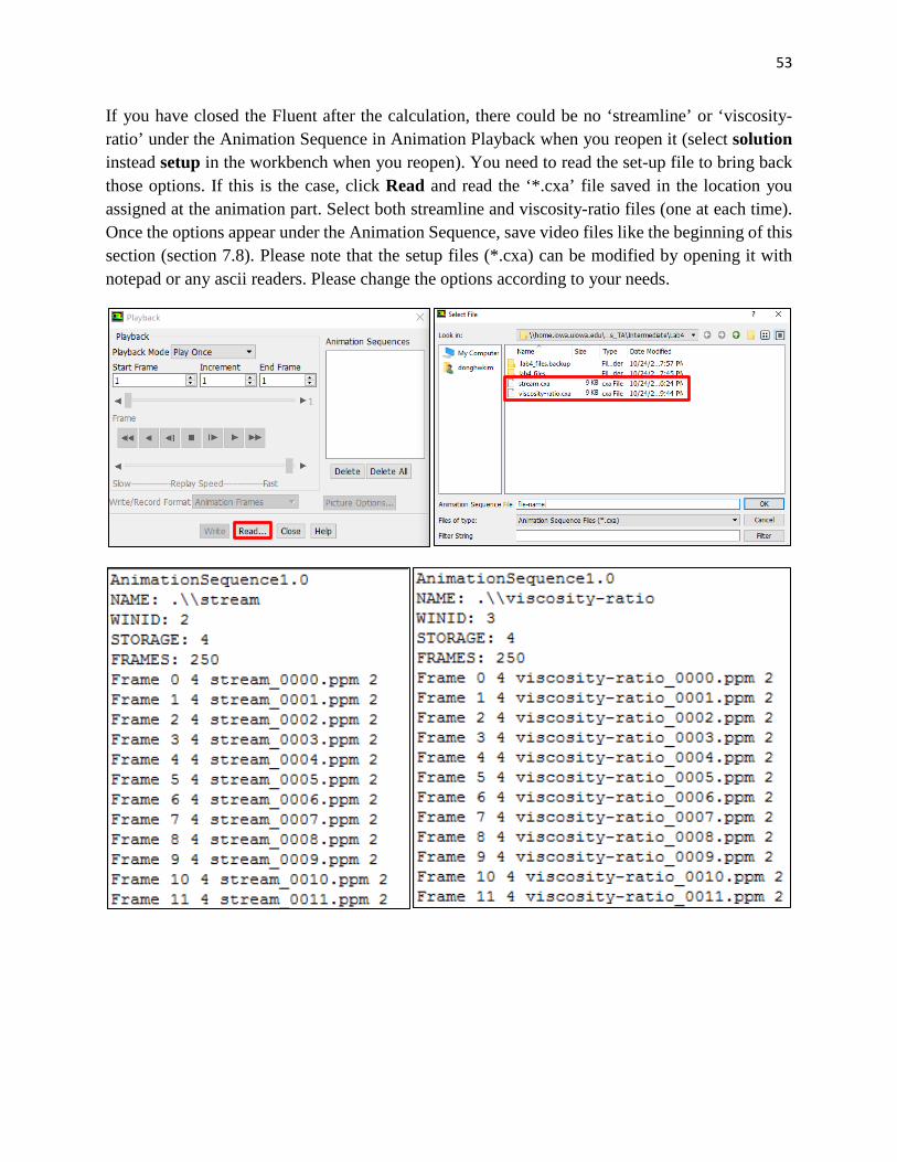
If you have closed the Fluent after the calculation, there could be no ‘streamline’ or ‘viscosity-ratio’ under the Animation Sequence in Animation Playback when you reopen it (select solution instead setup in the workbench when you reopen). You need to read the set-up file to bring back those options. If this is the case, click Read and read the ‘*.cxa’ file saved in the location you assigned at the animation part. Select both streamline and viscosity-ratio files (one at each time). Once the options appear under the Animation Sequence, save video files like the beginning of this section (section 7.8). Please note that the setup files (*.cxa) can be modified by opening it with notepad or any ascii readers. Please change the options according to your needs.

54

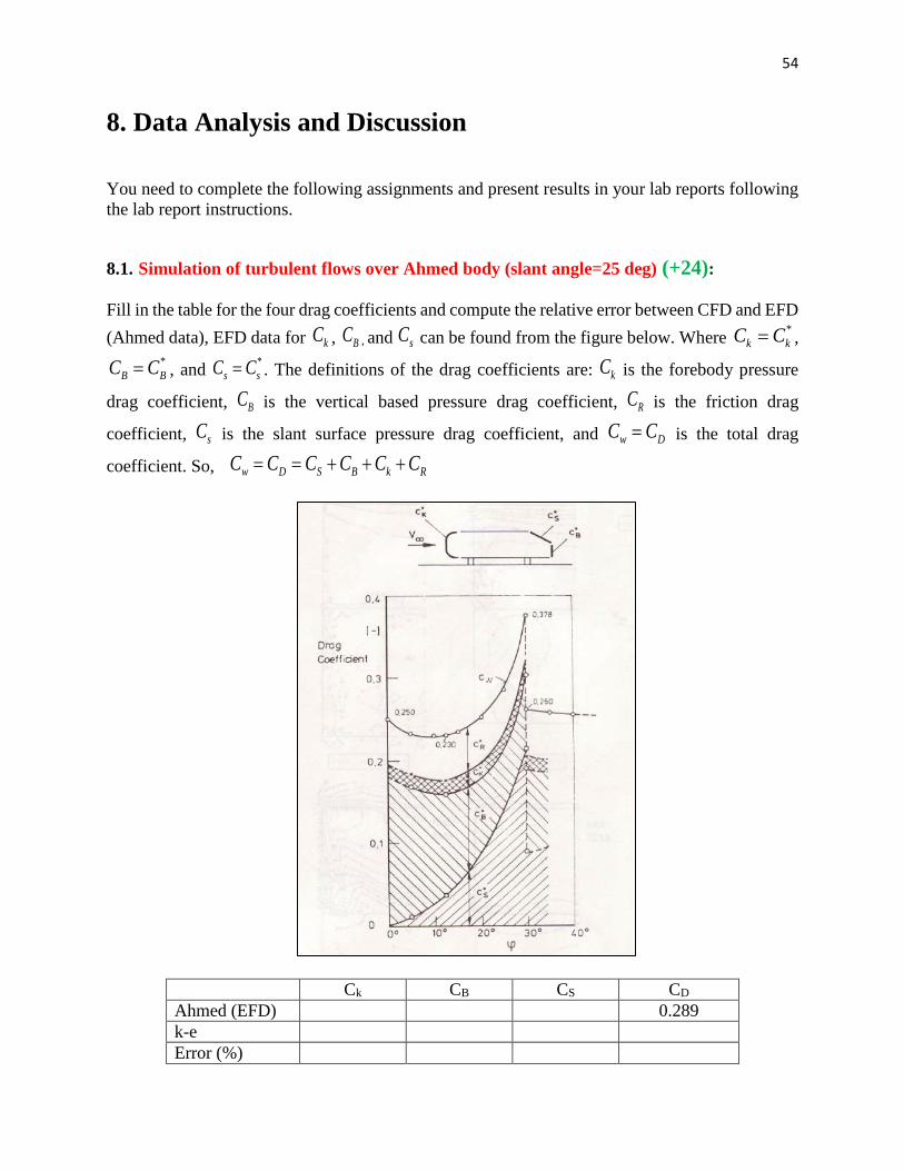
8. Data Analysis and Discussion

You need to complete the following assignments and present results in your lab reports following the lab report instructions.

8.1. Simulation of turbulent flows over Ahmed body (slant angle=25 deg) (+24): Fill in the table for the four drag coefficients and compute the relative error between CFD and EFD (Ahmed data), EFD data for kC , BC , and sC can be found from the figure below. Where *

k kC C= , *

B BC C= , and *s sC C= . The definitions of the drag coefficients are: kC is the forebody pressure

drag coefficient, BC is the vertical based pressure drag coefficient, RC is the friction drag

coefficient, sC is the slant surface pressure drag coefficient, and w DC C= is the total drag

coefficient. So, w D S B k RC C C C C C= = + + +

Ck CB CS CD Ahmed (EFD) 0.289 k-e Error (%)

55

Questions (+21): • Do you observe separations in the wake region (use streamlines)? If yes, where is the

location of separation point? • What is the Strouhal number based on the shedding frequency (CD vs. time), the height of

the Ahmed body and the inlet velocity? Note: the shedding frequency f=1/T where T is the typical period of the oscillation of CD that can be evaluated using the peaks between 0.1<time<0.14.

• Figures need to be reported: (1) XY plots for residual history, (2) modified U vs. y-by-h (with EFD), (3) Modified-TKE vs. y-by-h, (4) time history of drag coefficient, (5) Contour of pressure, (6) contour of velocity magnitude, (7) velocity vectors, (8) 3 or 4 snapshots of animations for turbulent-viscosity-ratio and streamlines (hints: you can use <<Alt+print Screen>> during the play of the animations).

• Data need to be reported: the above table with values.

56

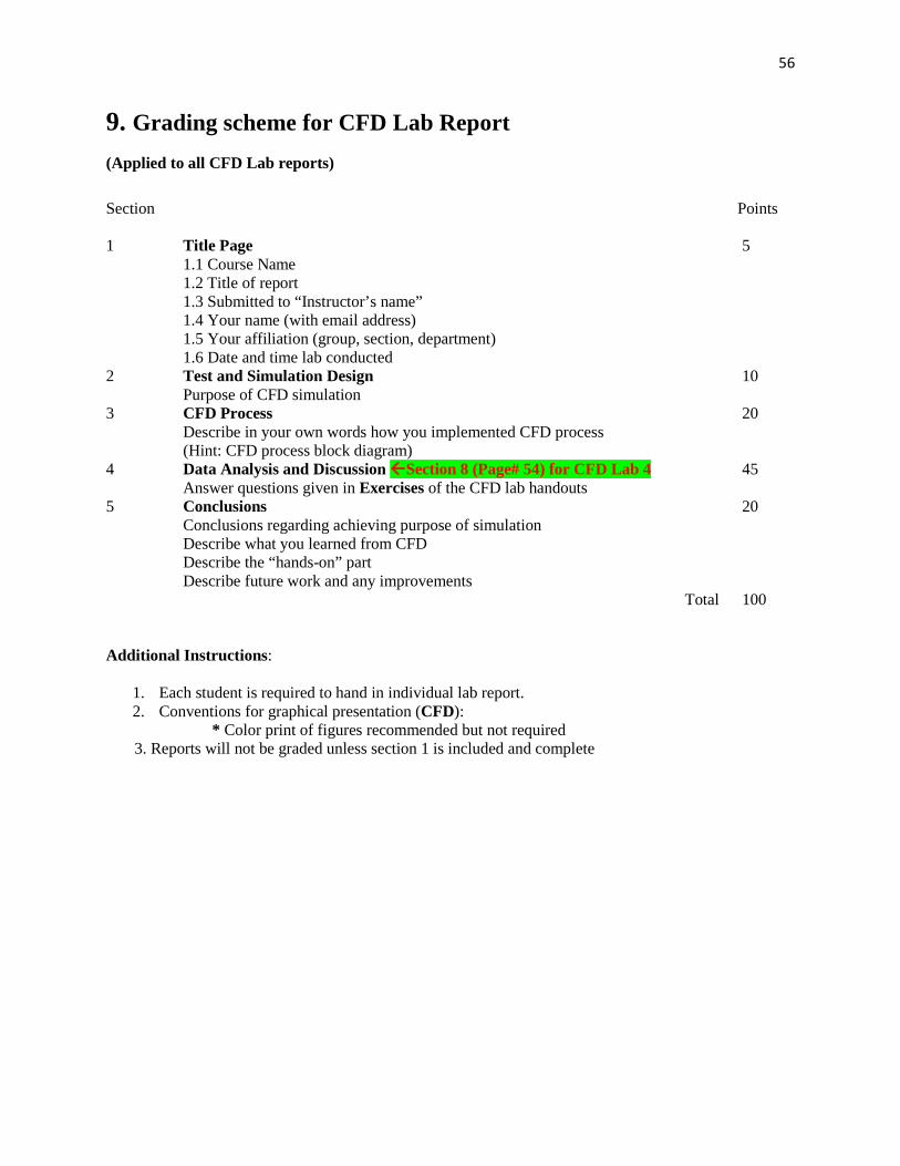
9. Grading scheme for CFD Lab Report (Applied to all CFD Lab reports)

Section Points 1 Title Page 5 1.1 Course Name 1.2 Title of report 1.3 Submitted to “Instructor’s name” 1.4 Your name (with email address) 1.5 Your affiliation (group, section, department) 1.6 Date and time lab conducted 2 Test and Simulation Design 10 Purpose of CFD simulation 3 CFD Process 20 Describe in your own words how you implemented CFD process (Hint: CFD process block diagram) 4 Data Analysis and Discussion Section 8 (Page# 54) for CFD Lab 4 45 Answer questions given in Exercises of the CFD lab handouts 5 Conclusions 20 Conclusions regarding achieving purpose of simulation Describe what you learned from CFD Describe the “hands-on” part Describe future work and any improvements Total 100 Additional Instructions:

1. Each student is required to hand in individual lab report. 2. Conventions for graphical presentation (CFD):

* Color print of figures recommended but not required 3. Reports will not be graded unless section 1 is included and complete