Simulation of the Martian dust cycle with the GFDL Mars GCMSimulation of the Martian dust cycle with the GFDL Mars GCM Shabari Basu and Mark I. Richardson Division of Geological and

Simulation of the Martian dust cycle with the GFDL Mars GCM

Shabari Basu and Mark I. RichardsonDivision of Geological and Planetary Sciences, California Institute of Technology, Pasadena, California, USA

R. John WilsonGeophysical Fluid Dynamics Laboratory, National Oceanic and Atmospheric Administration, Princeton, New Jersey, USA

Received 29 January 2004; revised 26 August 2004; accepted 16 September 2004; published 24 November 2004.

[1] The Martian seasonal dust cycle is examined with a general circulation model (GCM)that treats dust as a radiatively and dynamically interactive trace species. Dust injection isparameterized as being due to convective processes (such as dust devils) and model-resolved wind stresses. Size-dependent dust settling, transport by large-scale winds andsubgrid scale diffusion, and radiative heating due to the predicted dust distribution aretreated. Multiyear Viking and Mars Global Surveyor air temperature data are used toquantitatively assess the simulations. Varying the three free parameters for the two dustinjection schemes (rate parameters for the two schemes and a threshold for wind-stresslifting), we find that the highly repeatable northern spring and summer temperatures canbe reproduced by the model if the background dust haze is supplied by either convectivelifting or by stress lifting with a very low threshold and a low injection rate. Dust injectiondue to high-threshold, high-rate stress lifting must be added to these to generatespontaneous and variable dust storms. In order to supply the background haze, widespreadand ongoing lifting is required by the model. Imaging data provide a viable candidatemechanism for convective lifting, in the form of dust devils. However, observednonconvective lifting systems (local storms, etc.) appear insufficiently frequent andwidespread to satisfy the role. On the basis of the model results and thermal and imagingdata, we suggest that the background dust haze on Mars is maintained by convectiveprocesses, specifically, dust devils. Combining the convective scheme and high-thresholdstress lifting, we obtain a ‘‘best fit’’ multiyear simulation, which produces a realisticthermal state in northern spring and summer and, for the first time, spontaneous andinterannually variable global dust storms. INDEX TERMS: 6225 Planetology: Solar System

Objects: Mars; 5445 Planetology: Solid Surface Planets: Meteorology (3346); 5409 Planetology: Solid Surface

Planets: Atmospheres—structure and dynamics; 3319 Meteorology and Atmospheric Dynamics: General

circulation; 0305 Atmospheric Composition and Structure: Aerosols and particles (0345, 4801); KEYWORDS:

climate, dust, Mars

Citation: Basu, S., M. I. Richardson, and R. J. Wilson (2004), Simulation of the Martian dust cycle with the GFDL Mars GCM,

J. Geophys. Res., 109, E11006, doi:10.1029/2004JE002243.

1. Introduction

[2] Atmospheric dust is a very important component ofthe Martian climate system. The suspended mineral aerosolinteracts with both visible and infrared radiation, andthrough this interaction, modifies atmospheric heating rates[Gierasch and Goody, 1968; Kahn et al., 1992]. A richpotential for feedback exists due to the nonlinear relation-ship between the dust distribution, heating rates, and theatmospheric circulation that transports dust. The mostdramatic example of such feedback is the Martian globaldust storm, which over a matter of weeks can completelyenshroud the planet with haze [Leovy et al., 1972; Briggs etal., 1979; Martin and Richardson, 1993; Smith et al., 2002].

Of likely equal or greater importance for the mean climateof Mars is the control of the perpetual, but seasonallyvarying, ‘‘background’’ haze of dust. Models suggest thatthis haze produces at minimum roughly 5–10K of warmingin midlevel air temperatures compared to a clear atmo-sphere. The means by which this haze is maintained isunknown, but it now seems unlikely that it is maintained byslow fallout of dust following global dust storms: the highdegree of repeatability of air temperatures in northern springand summer [Richardson, 1998; Clancy et al., 2000; Liu etal., 2003; Smith, 2004] contrasts sharply with the interan-nual variability of global storms.[3] The seasonal cycle of dust has been observed in a

number of ways. Air temperatures have been measured fromorbit discontinuously since 1971 [Hanel et al., 1972;Martin, 1981; Conrath et al., 2000; Liu et al., 2003; Smith,2004]. These data provide a powerful and highly quantita-

JOURNAL OF GEOPHYSICAL RESEARCH, VOL. 109, E11006, doi:10.1029/2004JE002243, 2004

Copyright 2004 by the American Geophysical Union.0148-0227/04/2004JE002243$09.00

E11006 1 of 25

tive constraint on the dust cycle, but one that is convolvedwith the seasonal cycle of insolation. Dust opacities havebeen directly measured from these same orbital platforms[Martin, 1986; Fenton et al., 1997; Smith et al., 2001; Liu etal., 2003; Smith, 2004] and for more limited periods fromthe ground [Colburn et al., 1989; see also Toigo andRichardson, 2000; Smith and Lemmon, 1999]. Germane tothe issue of dust injection to support this annual cycle ofhaze are orbiter imaging of dust storms and dust devils.Local and regional dust storms have been observed from theViking Orbiter camera [Briggs et al., 1979], and mostrecently from the Mars Global Surveyor (MGS) MarsOrbiter Camera (MOC) [Cantor et al., 2001]. The coverageand resolution of MOC is such that the catalog of local andregional storms provided by Cantor et al. [2001] nowprovides a good climatology for a limited portion of oneyear. Dust devils have been observed in Viking Orbiterimages [Thomas and Gierasch, 1985], Mars Pathfindermeteorological and imaging data [Murphy and Nelli,2002; Metzger et al., 1999; Ferri et al., 2003], and MOCimages [Malin and Edgett, 2001; Cantor et al., 2002; Fisheret al., 2002].[4] Dust is included in all modern numerical models of the

Martian atmosphere, but usually as a prescribed opacity. Thisopacity is either held constant over the course of a givensimulation [Haberle et al., 1993, 2003] or prescribed to varyas a fixed function of season [Forget et al., 1999]. Suchapproaches are valuable as they allow the dust to be con-trolled as a free parameter when investigating a variety ofatmospheric phenomena. However, these approaches areobviously very limiting when it comes to examining the dustcycle itself. Interactive dust experiments, which involve thecoupling between the modeled winds, the dust distribution,and the calculation of atmospheric radiative heating rateswere first undertaken in General Circulation Models (GCM)in the mid-1990s [Murphy et al., 1990;Wilson, 1997]. Thesestudies were directly focused on the simulation of forcedglobal dust storms and resulting polar warming phenomena;prescribed surface sources of dust were used to trigger thestorms. Annual and interannual GCM simulations describedby Fenton and Richardson [2001], Richardson and Wilson[2002], and Richardson et al. [2002] used interactive dustwith an injection scheme based on surface-atmosphere tem-perature differences to simulate the seasonal cycle of non-dust-storm opacities and air temperature, performing well incomparison with observations [Richardson and Wilson,2002]. However, simulation of large dust storms hasremained the key focus of GCM dust studies to the presenttime. Most recently, Newman et al. [2002a, 2002b] imple-mented a set of interactive dust injection parameterizations,allowing interactions between the circulation, radiativeenvironment, and dust injection to be examined for the firsttime. Critically, this allowed dust injection and dust storms tobe generated as prognostic, ‘‘emergent’’ features of eachsimulation (in contrast to the ‘‘forced’’ nature of previousstudies). The Newman et al. [2002b] simulations generatedstorms similar to the 1999 ‘‘flushing storm’’ event observedby MGS [Cantor et al., 2001; Smith et al., 2001; Liu et al.,2003], likely due to the mechanism described byWang et al.[2003].[5] In future papers describing our studies, the dynamics

of global dust storms and their interannual variability will

be a major focus. However, in order to generate meaningfulsimulations of global dust storms, we believe it is crucial toproperly simulate the ‘‘background’’ state from which thesestorms are spawned. The reason for this, as describedfurther in a companion paper (S. Basu et al., manuscriptin preparation, 2004) (hereinafter referred to as B04), is thatthe background dustiness of the atmosphere strongly medi-ates the response of the atmospheric circulation to a givenamount of injected dust, as would be expected as a possibleoutcome for such a complex nonlinear system. This meansthat one could develop major storms too easily, or with toogreat a difficulty if the background state of the model isincorrectly (unrealistically) defined. Conversely, generationof a global dust storm in southern summer is meaningless ifas a natural consequence of the required dust injectionparameters, the model generates global dust storms innorthern summer, which is inconsistent with observations[Newman et al., 2002b].[6] Aside from its control of dust storm genesis, the

seasonally varying haze is a critical component of climateon Mars, moderating mean air temperatures and thecorresponding circulation. Attaining understanding of themechanisms controlling this cycle is critical if we are toexamine how Martian climate may have differed in the pastwhen forced by different patterns of insolation (such asassociated with changes in obliquity [Kieffer and Zent,1992]). Despite its direct and indirect importance, relativelylittle effort has been expended directly studying the ‘‘back-ground’’ seasonal cycle of dust and hence air temperatureswithout prescription. This paper focuses on this cycle.[7] This study takes advantage of dust injection parame-

terizations inspired by those developed and used byNewman et al. [2002a]. These schemes focus on twoinjection mechanisms: lifting by convective processes(based on a thermodynamic theory of dust devils), andlifting directly related to the model resolved winds. Theseschemes are still quite primitive in the sense that their scaledependence has not been exhaustively studied. As such, wesee this work as a first explorative step. In this light, weuse only three free parameters to control the schemes, withthe hope that the scale dependence is folded into theseconstants. As described in section 3, these free parametersare injection rate coefficients applied to convective andwind stress lifting, and a stress-threshold for wind stresslifting. We have extensively explored the phase-space ofthese free parameters, simultaneously targeting a realisticbackground (non-dust-storm) climate and generation ofrealistic global dust storms. Realism in the former case istested through the use of observed global air temperatures asa quantitative constraint. Realism in this latter case isdefined as generation of spontaneous and interannuallyvariable global dust storms in southern spring and summer(and not in northern spring and summer). The twin require-ments of continuous haze and distinctly noncontinuousdust storm generation places constraints on the model dustinjection parameters that would not be in force if eitherrequirement were imposed alone. The solution that arises inthe model is that while stress lifting could create either abackground haze or global storms, it cannot do bothsimultaneously with the same injection parameters. Con-versely, dust devil injection cannot generate spontaneousand variable storms regardless of the rate coefficient value.

E11006 BASU ET AL.: SIMULATION OF THE MARTIAN DUST CYCLE

2 of 25

E11006

As a result, an idea that emerges in this paper, is one of anatural separation between the roles of convective and windstress lifting. However, it seems plausible that convectivelifting is not important and that two or more different sets ofstress-lifting parameter values could be used simultaneouslyinstead. We examine both hypotheses in light of availableobservations, which appear to favor convective (and spe-cifically dust devil) supply over supply by local dust stormsor other wind stress related lifting.[8] In this paper, we provide a brief introduction to the

observational constraints, and then proceed to describe theGeophysical Fluid Dynamics Laboratory (GFDL) MarsGCM, and the dust lifting schemes specifically added forthis study. The model is then used to explore the areas ofphase space wherein a realistic cycle of background dustopacity (as gauged by the air temperatures) is obtained. Theresults of our experiments suggest that a steady (yet slowly,seasonally varying) and widespread source is necessary.This widespread and persistent source can be generated byconvective or wind stress driven sources. We will argue thatobservational constraints favor the convective source, in theform of widespread dust devil activity, though this is notconclusive, and further effort needs to be applied to obser-vationally constrain the roles of the potential steady andwidespread sources. In the latter part of this paper, we pick aset of dust lifting parameters that provide a ‘‘best fit’’ to theseasonal air temperature cycle, and that also yield interann-ually variable, spontaneous global dust storms in southernspring and summer. The non-dust-storm seasonal cycle ofthis simulation is examined in detail and compared withobservations. Finally, we look at the patterns of net dustlifting generated by this model for current orbital parame-ters. These simulations provide by far the best modelestimates of net dust lifting/deposition to date since themodel uses a fully interactive dust cycle and this cycle hasbeen strongly constrained by the thermal observations.

2. Observations

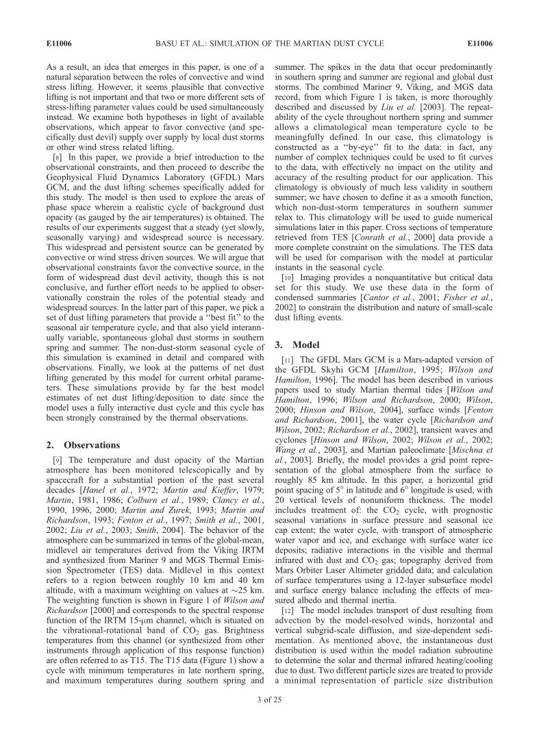
[9] The temperature and dust opacity of the Martianatmosphere has been monitored telescopically and byspacecraft for a substantial portion of the past severaldecades [Hanel et al., 1972; Martin and Kieffer, 1979;Martin, 1981, 1986; Colburn et al., 1989; Clancy et al.,1990, 1996, 2000; Martin and Zurek, 1993; Martin andRichardson, 1993; Fenton et al., 1997; Smith et al., 2001,2002; Liu et al., 2003; Smith, 2004]. The behavior of theatmosphere can be summarized in terms of the global-mean,midlevel air temperatures derived from the Viking IRTMand synthesized from Mariner 9 and MGS Thermal Emis-sion Spectrometer (TES) data. Midlevel in this contextrefers to a region between roughly 10 km and 40 kmaltitude, with a maximum weighting on values at �25 km.The weighting function is shown in Figure 1 of Wilson andRichardson [2000] and corresponds to the spectral responsefunction of the IRTM 15-mm channel, which is situated onthe vibrational-rotational band of CO2 gas. Brightnesstemperatures from this channel (or synthesized from otherinstruments through application of this response function)are often referred to as T15. The T15 data (Figure 1) show acycle with minimum temperatures in late northern spring,and maximum temperatures during southern spring and

summer. The spikes in the data that occur predominantlyin southern spring and summer are regional and global duststorms. The combined Mariner 9, Viking, and MGS datarecord, from which Figure 1 is taken, is more thoroughlydescribed and discussed by Liu et al. [2003]. The repeat-ability of the cycle throughout northern spring and summerallows a climatological mean temperature cycle to bemeaningfully defined. In our case, this climatology isconstructed as a ‘‘by-eye’’ fit to the data: in fact, anynumber of complex techniques could be used to fit curvesto the data, with effectively no impact on the utility andaccuracy of the resulting product for our application. Thisclimatology is obviously of much less validity in southernsummer; we have chosen to define it as a smooth function,which non-dust-storm temperatures in southern summerrelax to. This climatology will be used to guide numericalsimulations later in this paper. Cross sections of temperatureretrieved from TES [Conrath et al., 2000] data provide amore complete constraint on the simulations. The TES datawill be used for comparison with the model at particularinstants in the seasonal cycle.[10] Imaging provides a nonquantitative but critical data

set for this study. We use these data in the form ofcondensed summaries [Cantor et al., 2001; Fisher et al.,2002] to constrain the distribution and nature of small-scaledust lifting events.

3. Model

[11] The GFDL Mars GCM is a Mars-adapted version ofthe GFDL Skyhi GCM [Hamilton, 1995; Wilson andHamilton, 1996]. The model has been described in variouspapers used to study Martian thermal tides [Wilson andHamilton, 1996; Wilson and Richardson, 2000; Wilson,2000; Hinson and Wilson, 2004], surface winds [Fentonand Richardson, 2001], the water cycle [Richardson andWilson, 2002; Richardson et al., 2002], transient waves andcyclones [Hinson and Wilson, 2002; Wilson et al., 2002;Wang et al., 2003], and Martian paleoclimate [Mischna etal., 2003]. Briefly, the model provides a grid point repre-sentation of the global atmosphere from the surface toroughly 85 km altitude. In this paper, a horizontal gridpoint spacing of 5� in latitude and 6� longitude is used, with20 vertical levels of nonuniform thickness. The modelincludes treatment of: the CO2 cycle, with prognosticseasonal variations in surface pressure and seasonal icecap extent; the water cycle, with transport of atmosphericwater vapor and ice, and exchange with surface water icedeposits; radiative interactions in the visible and thermalinfrared with dust and CO2 gas; topography derived fromMars Orbiter Laser Altimeter gridded data; and calculationof surface temperatures using a 12-layer subsurface modeland surface energy balance including the effects of mea-sured albedo and thermal inertia.[12] The model includes transport of dust resulting from

advection by the model-resolved winds, horizontal andvertical subgrid-scale diffusion, and size-dependent sedi-mentation. As mentioned above, the instantaneous dustdistribution is used within the model radiation subroutineto determine the solar and thermal infrared heating/coolingdue to dust. Two different particle sizes are treated to providea minimal representation of particle size distribution


3 of 25

E11006

changes. The radiation scheme treats dust as an absorbersand scatterers in the visible (with a single scattering albedo of0.92). In the thermal infrared, only absorption and emissionare considered (see Wilson and Hamilton [1996], and notethat in some versions of the GFDL model, a more detailedradiative scheme has been used [Hinson and Wilson, 2004]).Using fixed dust distributions or finely tuned interactivedust injection, it has proven possible to simultaneously fitair temperatures and observed TES dust opacities.[13] The new components of the model for this study

relate to dust injection. Dust injection in the real Martianatmosphere takes place in association with motions on avariety of scales, running the gamut from synoptic motionsto those associated with boundary layer turbulence. Obvi-ously, this full spectrum cannot be explicitly treated in a

model with grid spacing of order hundreds of kilometers.We therefore are faced with choices about how we param-eterize lifting processes that are not model resolved. Imag-ing observations suggest that dust lifting is at least sensitiveto the ‘‘mean wind’’ (on some scale) and to convectivemotions. The former is indicated, for example, by duststreaks and the latter by dust devils captured in spacecraftimages [e.g., Fenton and Richardson, 2001; Cantor et al.,2002]. On this basis, it seems plausible to base liftingaround schemes that are related to the strength of theresolved wind (or actually the imparted stress) and the vigorof boundary layer convection. This is not necessarilyunique; on the mesoscale and microscale, the ‘‘mean wind’’can be modified by local topography and surface thermalcontrasts such that a number of different stresses are

Figure 1. The seasonal variation of midlevel atmospheric temperatures between 40�S and 40�N derivedfrom spacecraft infrared observations and from selected GCM simulations. The data are taken from theViking Infrared Thermal Mapper (IRTM) 15-mm channel (corrected [see Wilson and Richardson, 2000;Liu et al., 2003]) and from the Mars Global Surveyor Thermal Emission Spectrometer (TES) spectra afterconvolution with the IRTM 15-mm channel spectral response function. The corresponding IRTM 15-mmchannel weighting function peaks at roughly 25 km, with contribution primarily from 10 to 40 km. Thisweighting function has been applied to the GCM output for optimal comparison with data. A meanseasonal climatology of air temperature (the ‘‘background cycle,’’ which excludes large dust stormeffects) has been defined via a ‘‘by-eye’’ fit to the observations. GCM simulations corresponding to the‘‘best fit’’ dust devil source, and a simulation with no atmospheric dust opacity. The background hazegenerates about 5–10K of warming compared to a clear atmosphere. Note that the minima near thesolstices correspond to the relative deposition of more solar heating poleward of 40� at these seasons thanduring the equinoxes.


4 of 25

E11006

working within a single GCM grid cell. It again seemsplausible that these subresolved winds would scale withthe strength of the grid-resolved mean wind, but it is notnecessarily so (profoundly nonlinear acceleration processescan be at work in some circumstances [Magalhaes andYoung, 1995]). A detailed mesoscale modeling study isnecessary to address the importance of microscale andmesoscale influences on ‘‘mean wind’’ dust lifting. In anycase, for our initial study of the Martian dust cycle, it wouldseem to be prudent to devise parameterizations that representsome dependence on mean winds and on convective vigor,while at the same time, keeping the schemes sufficientlysimple that they can readily be comprehended. No doubtmore complex and realistic schemes will emerge in thefuture; their impact in changing the results of this study (ornot) will be of great importance for developing an increas-ingly complete understanding of the Martian dust cycle.[14] The two schemes used in this paper are inspired by

those first implemented in a GCM by Newman et al. [2002a,2002b]. The first relates lifting to the model-resolved windvia relationships worked out in wind tunnel experiments[e.g., Shao, 2001]. The second uses the Renno et al. [1998]thermodynamic theory of dust devils as the basis forpredicting convective lifting. The representations of liftingare incomplete in that there is no scale dependence (noexplicit dependence on grid spacing) such that the schemesneed to be adjusted for model runs with different resolution.Our experience suggests that the stress scheme requireslarger-scale correction than does the convective scheme. Inany case, parameterizations in the future should account forresolution variations. More importantly, we have intention-ally chosen to take only the functional forms for the liftingschemes from wind tunnel results and from theory: We havechosen to use free parameters to scale the functions as anactive part of our experiments. We feel this is an honestreflection of our ignorance of the microscale processesinvolved in dust lifting. Tunable free parameters allow usto sidestep this ignorance (or rather contain this ignorancewithin a parameter, whose meaning may be examined atsome later time). The connection to reality is provided bywell-known constraints: the large-scale atmospheric temper-atures and the functional forms of the lifting parameter-izations that are based on the observed physics. In the nexttwo subsections, we describe these parameterizations.

3.1. Convective (‘‘Dust Devil’’) Parameterization

[15] The parameterization of small-scale convectivemotions is based on thermodynamic theory of dust devils[Renno et al., 1998]. This choice is rooted in our bias thatdust devils are likely the dominant form of convectivelifting (not proven and in need of observational testing).However, this choice is actually quite general and reason-able since the functional form relates lifting to the stabilityof the boundary layer and the vigor of heat transfer betweenthe surface and the atmosphere: more generally, the schemelinks lifting to the strength of convective motions and assuch should capture the nature of any convective lifting.[16] The convective scheme (hereinafter generally

referred to as the dust devil lifting or DDL scheme) isimplemented using a simple fixed function that is based onthe thermodynamics of dust devils [Renno et al., 1998]. TheRenno et al. [1998] heat engine theory of dust devils relates

the dust lifting intensity to the sensible heat input, Fheat, atthe surface and the thermodynamic efficiency, h, whichdepends on the depth of the Planetary Boundary Layer(PBL). The lifting rate is then related to the intensity withthe application of a multiplicative injection rate constant,RDDL. This free parameter allows for potential (and likely)offsets between the lifting of a single dust devil respondingto a local heat flux and thermodynamic efficiency, and thatof an ensemble of dust devils responding to a range of localenvironments within a model grid box of roughly 300 kmwidth, and with grid-average values of sensible heat fluxand thermodynamic efficiency. Since this multiplier isunknown a priori, we use it as one of the available tuningparameters in the model, with the seasonal cycle of airtemperatures defining the ‘‘target’’ for tuning, as describedlater in this paper. The dust devil injection function isspecifically defined as

FDDL ¼ RDDL � Fheat � h:

The dust injection rate scheme is implemented in the GCMsuch that, so long as the function is positive at a given gridpoint, there is some lifting at that grid point; there is noactivation threshold defined for DDL. There is no inherenttime/space variation or randomness in this function.[17] The relationship between the GCM DDL and the

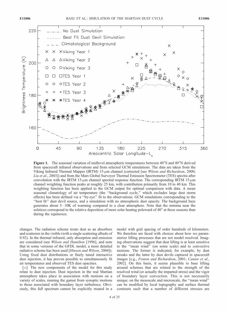
model variables upon which it depends are illustrated inFigure 2. These output are taken from a specific grid pointin the model at a specific time (lat, lon, season), but arerepresentative of the behavior of the DDL scheme generallywithin the model. The ground temperature (Figure 2a)provides a direct drive for the sensible heat flux betweenthe surface and the atmosphere, Fheat (Figure 2b). As such,there is a clear diurnal cycle of sensible heat flux that is inphase with that of the surface temperature. The h function(Figure 2c) is related to the ground temperature through theconvective boundary layer depth (Figure 2d), which has asimilar shape to the diurnal cycle of surf ace temperature,but offset by a few hours to later local times (since airtemperatures lag the surface temperature). The combinationof the sensible heat flux and the h function result in a shift inpeak dust devil activity, and hence dust devil lifting in thisparameterization, to the early afternoon. This phase shift isin keeping with (results directly from) the predictions of thethermodynamic theory [Renno et al., 1998]. Clearing ofdust from the atmosphere is accomplished in the model bygravitational sedimentation. The settling associated with theparticle sizes used in this study have been shown to allowthe atmosphere to relax back from prescribed dust storms ina realistic manner [see Wilson and Richardson, 1999].[18] The spatial relationship between the net dust injec-

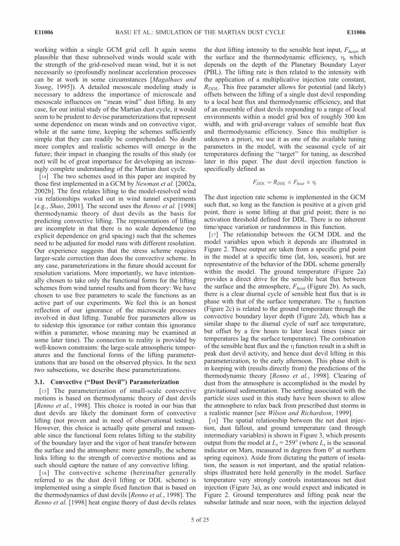
tion, dust fallout, and ground temperature (and throughintermediary variables) is shown in Figure 3, which presentsoutput from the model at Ls = 259� (where Ls is the seasonalindicator on Mars, measured in degrees from 0� at northernspring equinox). Aside from dictating the pattern of insola-tion, the season is not important, and the spatial relation-ships illustrated here hold generally in the model. Surfacetemperature very strongly controls instantaneous net dustinjection (Figure 3a), as one would expect and indicated inFigure 2. Ground temperatures and lifting peak near thesubsolar latitude and near noon, with the injection delayed


5 of 25

E11006

slightly with respect to ground temperatures. The spatialpattern of convective PBL height is illustrated in Figure 3b.This is similar to plots for other Mars GCMs [e.g., Haberleet al., 1993]. The PBL parameterization in the GCM doesnot make an explicit prediction of the PBL height, so thisvalue must be calculated. This is done on each time step andfor each grid point by deriving the potential temperature foreach layer in each model atmospheric column (i.e., at alllevels above each grid point) for the predicted air temper-atures prior to convective adjustment. Working upwardfrom the surface, when a layer is found whose potentialtemperature exceeds that of the near surface layer, thepressure of the interface between this higher potentialtemperature layer and the one below it is recorded as the

local PBL top pressure. PBL geometric height is easilyrecovered by upward hydrostatic integration.[19] The sensible heat flux (Figure 3c) and h function

(Figure 3d) patterns follow those of the ground temperatureand PBL depth, much as would be expected from Figure 1.The deviations from a smooth spatial pattern, with valuesmonotonically falling with increasing latitudinal and longi-tudinal distance from the subsolar point reflect surfacevariations in the thermal inertia and albedo of the surfacevia their influence upon ground temperature. In addition, thesensible heat flux pattern is influenced by the circulationthrough the surface wind stress. These functions combine toyield the net DDL, illustrated in Figure 3e. This figureprovides a map of the model-predicted dust devil activity

Figure 2. The relationship between predicted dust devil lifting (DDL) rates and various model variablesas a function of local time for a point at 0� longitude and 0� latitude for Ls = 259�. (a) Solar heating of thesurface and subsequent convective motions to shed this heat provide the primary drive for dust devilactivity. (b) The sensible heat flux peaks earlier than the ground temperature peak (i.e., in the morning).At this time of day there is greatest contrast between the surface and atmospheric temperatures andconsequently the strongest convective drive. (c and d) The thermodynamic theory of dust devils [Rennoet al., 1998] suggests a strong dependence upon an ‘‘efficiency function’’ that is itself dependent upon thedepth of the planetary boundary layer (PBL). The PBL depth peaks later than the ground temperaturemaximum (in the afternoon) as it takes time for the PBL to entrain successively higher portions of the freeatmosphere. (e) The resulting dust devil injection is a convolution of the sensible heat flux and the PBLdepth. (f ) The net effect of dust devils can be determined only when the dust fallout rate is alsoconsidered. While the fallout is about an order of magnitude lower, the fallout never falls below 80% ofits maximum value (at this location), providing a very steady sink. The instantaneous spatial pattern,shown in Figure 3, is therefore much smoother than that of injection.


6 of 25

E11006

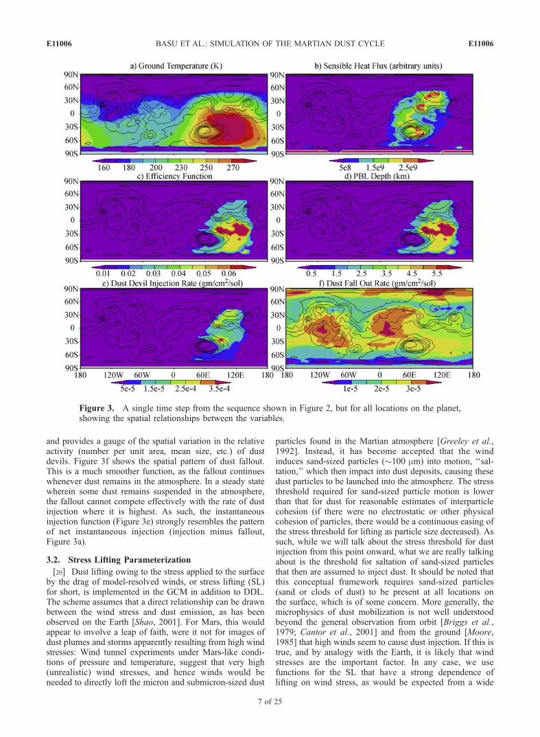
and provides a gauge of the spatial variation in the relativeactivity (number per unit area, mean size, etc.) of dustdevils. Figure 3f shows the spatial pattern of dust fallout.This is a much smoother function, as the fallout continueswhenever dust remains in the atmosphere. In a steady statewherein some dust remains suspended in the atmosphere,the fallout cannot compete effectively with the rate of dustinjection where it is highest. As such, the instantaneousinjection function (Figure 3e) strongly resembles the patternof net instantaneous injection (injection minus fallout,Figure 3a).

3.2. Stress Lifting Parameterization

[20] Dust lifting owing to the stress applied to the surfaceby the drag of model-resolved winds, or stress lifting (SL)for short, is implemented in the GCM in addition to DDL.The scheme assumes that a direct relationship can be drawnbetween the wind stress and dust emission, as has beenobserved on the Earth [Shao, 2001]. For Mars, this wouldappear to involve a leap of faith, were it not for images ofdust plumes and storms apparently resulting from high windstresses: Wind tunnel experiments under Mars-like condi-tions of pressure and temperature, suggest that very high(unrealistic) wind stresses, and hence winds would beneeded to directly loft the micron and submicron-sized dust

particles found in the Martian atmosphere [Greeley et al.,1992]. Instead, it has become accepted that the windinduces sand-sized particles (�100 mm) into motion, ‘‘sal-tation,’’ which then impact into dust deposits, causing thesedust particles to be launched into the atmosphere. The stressthreshold required for sand-sized particle motion is lowerthan that for dust for reasonable estimates of interparticlecohesion (if there were no electrostatic or other physicalcohesion of particles, there would be a continuous easing ofthe stress threshold for lifting as particle size decreased). Assuch, while we will talk about the stress threshold for dustinjection from this point onward, what we are really talkingabout is the threshold for saltation of sand-sized particlesthat then are assumed to inject dust. It should be noted thatthis conceptual framework requires sand-sized particles(sand or clods of dust) to be present at all locations onthe surface, which is of some concern. More generally, themicrophysics of dust mobilization is not well understoodbeyond the general observation from orbit [Briggs et al.,1979; Cantor et al., 2001] and from the ground [Moore,1985] that high winds seem to cause dust injection. If this istrue, and by analogy with the Earth, it is likely that windstresses are the important factor. In any case, we usefunctions for the SL that have a strong dependence oflifting on wind stress, as would be expected from a wide

Figure 3. A single time step from the sequence shown in Figure 2, but for all locations on the planet,showing the spatial relationships between the variables.


7 of 25

E11006

variety of wind related lifting mechanisms, be it via salta-tion or direct lifting.[21] The parameterization generally used in this study

defines the dust injection flux FSL as follows:

FSL ¼ RSL � f Udrag

� �; u > uthresh;

FSL ¼ 0; u < uthresh;

where RSL is a multiplicative rate parameter, r is the airdensity,Udrag is the frictional velocity, and where f(Udrag) canbe a simple function of the wind velocity, u, boundary layereddy diffusivity, and the threshold wind speed, uthresh. SL isthreshold dependent; there is lifting only when the windstress t (t = rUdrag

2 ) is greater than tSL, the threshold windstress corresponding to uthresh. There is no dust lifting whenthe wind stress is below tSL. The threshold stress can be takenfrom wind tunnel experiments [see Greeley et al., 1992].However, due to concerns over the ability of any numericalatmospheric model to accurately predict the absolute valuesof surface stress, the possibility that wind tunnel experimentsmiss some important physics (such as electrostatic effects),and the applicability of local thresholds to the average windover modeled spatial scales of hundreds of kilometers, webelieve it more prudent to use the threshold as a freeparameter. Thus the activation threshold wind stress, tSL, andthe multiplicative injection rate factor RSL, yield two freeparameters associated with our dust SL scheme.[22] A variety of functional forms for f (Udrag) have been

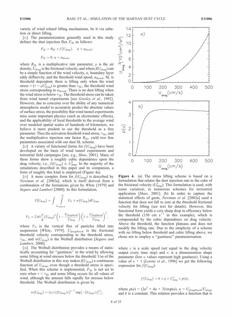
developed on the basis of wind tunnel experiments andterrestrial field campaigns [see, e.g., Shao, 2001]. Many ofthese forms show a roughly cubic dependence upon thedrag velocity, i.e., f (Udrag) / Udrag

3 . In the majority of thesimulations described in this paper and its companion, aform of roughly this kind is employed (Figure 4a).[23] A more complex form for f (Udrag) is described by

Newman et al. [2002a], which is itself derived from acombination of the formations given by White [1979] andSeguro and Lambert [2000]. In this formulation,

f Udrag

� �¼

Z Z1

Udragthresh

VN � w Udrag

� �dUdrag;

VN ¼ 2:61rg

Udrag

� �31� Udragthresh

Udrag

� �1þ Udragthresh

Udrag

� �2

;

where VN is the vertical flux of particles lifted intosuspension [White, 1979], Udragthresh is the frictionalthreshold velocity corresponding to the threshold stress,tSL, and w(Udrag) is the Weibull distribution [Seguro andLambert, 2000].[24] The Weibull distribution provides a means of statis-

tically accounting for ‘‘gustiness’’ in the wind by allowingsome lifting at wind stresses below the threshold. Use of theWeibull distribution in this way makes f(Udrag) a continuousfunction of Udrag, even though a threshold stress is speci-fied. When this scheme is implemented, FSL is not set tozero when t < tSL and some lifting occurs for all values ofwind, although the amount falls rapidly for stresses belowthreshold. The Weibull distribution is given by

w Udrag

� �¼ k=cð Þ Udrag=c

� �k�1exp � Udrag=c

� �k� �;

where c is a scale speed (set equal to the drag velocityoutput every time step) and k is a dimensionless shapeparameter (low k values represent high gustiness). Using avalue of k = 1 [Lorenz et al., 1996] we get the followingexpression for f (Udrag):

f Udrag

� �¼ k � r� U3

drag � p uð Þ;

where p(u) = (2u2 + 4u + 3)/exp(u), u = Udragthresh/Udrag,and k is a constant. This relation provides a function that is

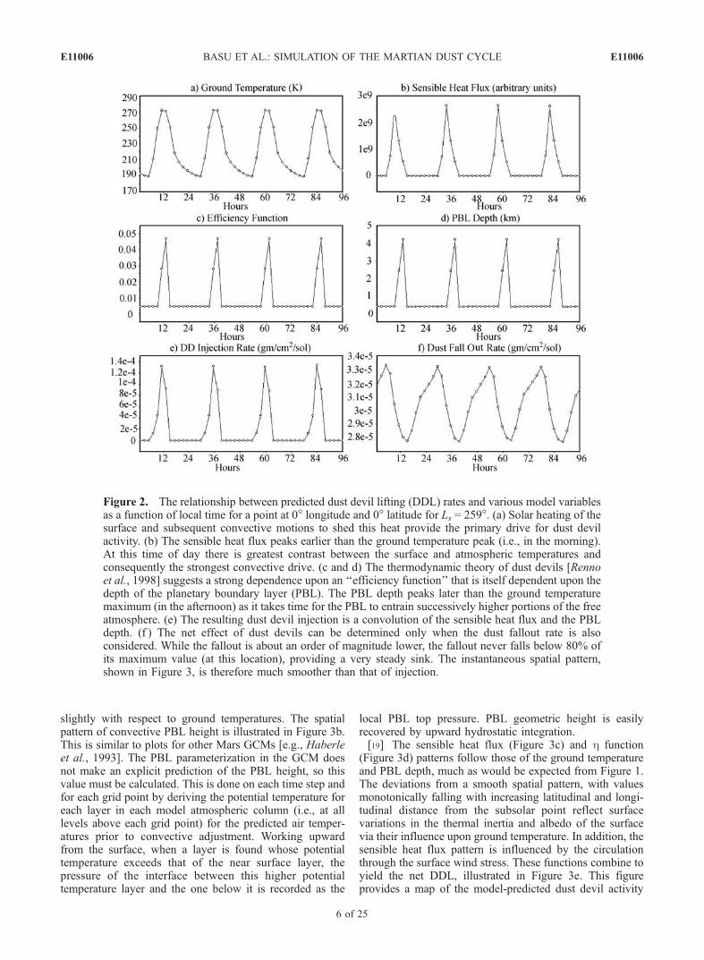
Figure 4. (a) The stress lifting scheme is based on aformulation that relates the dust injection rate to the cube ofthe frictional velocity (Udrag

3 ). This formulation is used, withsome variation, in numerous schemes for terrestrialapplication [Shao, 2001]. (b) In order to capture thestatistical effects of gusts, Newman et al. [2002a] used afunction that does not fall to zero at the threshold frictionalvelocity for lifting (see text for details). However, thisfunctional form yields a very sharp drop in efficiency belowthe threshold (150 cm s�1 in this example), which iscompounded by the cubic dependence on drag velocity.Above the threshold, the function plateaus and does notmodify the lifting rate. Due to the simplicity of a schemewith no lifting below threshold and cubic lifting above, wechose not to employ a ‘‘gustiness’’ parameterization.


8 of 25

E11006

zero for Udrag = 0, and grows, dominated by theexponential term, to a value at u = Udragthresh/Udrag = 1, atwhich the function essentially plateaus for Udrag >Udragthresh (Figure 4b). The prediction of some lifting forUdrag < Udragthesh with this function is an attempt to capturelifting due to gusts at scales not resolved by the model. Thevalue of k chosen determines how sharply lifting declines asthe Udrag decreases below the threshold.[25] In either case, for values of wind stress above the

threshold, the lifting rate is / Udrag3 and the only difference

is the sharpness of the stress threshold cut off for lifting forUdrag < Udragthesh. Partly because a very much simplerinterpretation of the results emerge if the threshold is sharp,partly because it seems useful to employ a physically simpleparameterization for a system that is poorly understood, andpartly because the observations in hand [e.g., Moore, 1985,Zurek et al., 1992] do not appear to readily support thewidespread, low-rate dust injection that the continuousscheme generates, we chose to use the simple, threshold-dependent, Udrag

3 scheme.[26] A consequence of the threshold-dependent scheme is

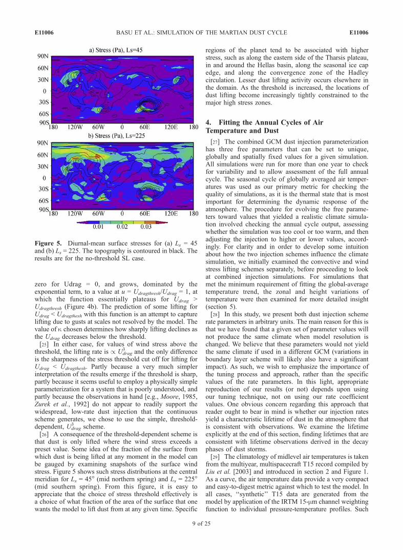
that dust is only lifted where the wind stress exceeds apreset value. Some idea of the fraction of the surface fromwhich dust is being lifted at any moment in the model canbe gauged by examining snapshots of the surface windstress. Figure 5 shows such stress distributions at the centralmeridian for Ls = 45� (mid northern spring) and Ls = 225�(mid southern spring). From this figure, it is easy toappreciate that the choice of stress threshold effectively isa choice of what fraction of the area of the surface that onewants the model to lift dust from at any given time. Specific

regions of the planet tend to be associated with higherstress, such as along the eastern side of the Tharsis plateau,in and around the Hellas basin, along the seasonal ice capedge, and along the convergence zone of the Hadleycirculation. Lesser dust lifting activity occurs elsewhere inthe domain. As the threshold is increased, the locations ofdust lifting become increasingly tightly constrained to themajor high stress zones.

4. Fitting the Annual Cycles of AirTemperature and Dust

[27] The combined GCM dust injection parameterizationhas three free parameters that can be set to unique,globally and spatially fixed values for a given simulation.All simulations were run for more than one year to checkfor variability and to allow assessment of the full annualcycle. The seasonal cycle of globally averaged air temper-atures was used as our primary metric for checking thequality of simulations, as it is the thermal state that is mostimportant for determining the dynamic response of theatmosphere. The procedure for evolving the free parame-ters toward values that yielded a realistic climate simula-tion involved checking the annual cycle output, assessingwhether the simulation was too cool or too warm, and thenadjusting the injection to higher or lower values, accord-ingly. For clarity and in order to develop some intuitionabout how the two injection schemes influence the climatesimulation, we initially examined the convective and windstress lifting schemes separately, before proceeding to lookat combined injection simulations. For simulations thatmet the minimum requirement of fitting the global-averagetemperature trend, the zonal and height variations oftemperature were then examined for more detailed insight(section 5).[28] In this study, we present both dust injection scheme

rate parameters in arbitrary units. The main reason for this isthat we have found that a given set of parameter values willnot produce the same climate when model resolution ischanged. We believe that these parameters would not yieldthe same climate if used in a different GCM (variations inboundary layer scheme will likely also have a significantimpact). As such, we wish to emphasize the importance ofthe tuning process and approach, rather than the specificvalues of the rate parameters. In this light, appropriatereproduction of our results (or not) depends upon usingour tuning technique, not on using our rate coefficientvalues. One obvious concern regarding this approach thatreader ought to bear in mind is whether our injection ratesyield a characteristic lifetime of dust in the atmosphere thatis consistent with observations. We examine the lifetimeexplicitly at the end of this section, finding lifetimes that areconsistent with lifetime observations derived in the decayphases of dust storms.[29] The climatology of midlevel air temperatures is taken

from the multiyear, multispacecraft T15 record compiled byLiu et al. [2003] and introduced in section 2 and Figure 1.As a curve, the air temperature data provide a very compactand easy-to-digest metric against which to test the model. Inall cases, ‘‘synthetic’’ T15 data are generated from themodel by application of the IRTM 15-mm channel weightingfunction to individual pressure-temperature profiles. Such

Figure 5. Diurnal-mean surface stresses for (a) Ls = 45and (b) Ls = 225. The topography is contoured in black. Theresults are for the no-threshold SL case.


9 of 25

E11006

model output have been shown by Wilson and Richardson[2000] and Richardson and Wilson [2002].

4.1. Dust Devil Source

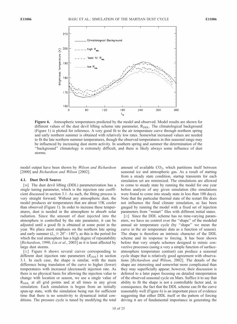
[30] The dust devil lifting (DDL) parameterization has asingle tuning parameter, which is the injection rate coeffi-cient discussed in section 3.1. As such, the fitting process isvery straight forward. Without any atmospheric dust, themodel produces air temperatures that are about 15K coolerthan observed (Figure 1). In order to increase these temper-atures, dust is needed in the atmosphere to absorb solarradiation. Since the amount of dust injected into theatmosphere is controlled by the rate parameter, it can beadjusted until a good fit is obtained at some point in theyear. We place most emphasis on the northern late springand early summer (Ls ffi 20�–140�), as this is the period forwhich the real atmosphere has a high degree of repeatability[Richardson, 1998; Liu et al., 2003] as it is least affected bylarge dust storms.[31] Figure 6 shows several curves corresponding to

different dust injection rate parameters (RDDL) in section3.1. In each case, the shape is similar, with the maindifference being translation of the curve to higher (lower)temperatures with increased (decreased) injection rate. Asthere is no physical basis for allowing the injection value tochange with location or season, we use a single value ofRDDL at all grid points and at all times in any givensimulation. Each simulation is begun from an initiallyspun-up state, with the simulation being run for sufficienttime that there is no sensitivity to dynamical initial con-ditions. The pressure cycle is tuned by modifying the total

amount of available CO2, which partitions itself betweenseasonal ice and atmospheric gas. As a result of startingfrom a steady state condition, startup transients for eachsimulation set are minimized. The simulations are allowedto come to steady state by running the model for one yearbefore analysis of any given simulation (the simulationswere found to come into steady state in less than 100 days).Note that the particular thermal state of the restart file doesnot influence the final climate simulation, as has beengauged by running the model with a fixed set of injectionparameters from ‘‘restart’’ files with different initial states.[32] Since the DDL scheme has no time-varying param-

eters, we have no control over the ‘‘shape’’ of the modeledannual air temperature cycle (by ‘‘shape’’ we mean thecurve in the air temperature data as a function of season).The shape is therefore an intrinsic character of the DDLscheme and its response to forcing. It has been shownbefore that very simple schemes designed to mimic con-vective processes (using a very a simple function of surface-atmosphere temperature contrast) can produce a seasonalcycle shape that is relatively good agreement with observa-tions [Richardson and Wilson, 2002]. The details of theshape are interesting and somewhat more complicated thanthey may superficially appear; however, their discussion isdeferred to a later paper focusing on detailed interpretationof the observed seasonal cycle on Mars. Suffice it to say thatability to fit the shape is not a controllable factor and, inconsequence, the fact that the DDL scheme can fit the curvereasonably well (Figure 6) is an important piece of evidencesuggesting that either DDL itself or the pattern of forcingdriving it are of fundamental importance in generating the

Figure 6. Atmospheric temperatures predicted by the model and observed. Model results are shown fordifferent values of the dust devil lifting scheme rate parameter, RDDL. The climatological background(Figure 1) is plotted for reference. A very good fit to the air temperature curve through northern springand early northern summer is obtained with relatively low rates. Somewhat increased values are neededto fit the late northern summer temperatures, though the observed temperatures in this seasonal range maybe influenced by increasing dust storm activity. In southern spring and summer the determination of the‘‘background’’ climatology is extremely difficult, and there is likely always some influence of duststorms.


10 of 25

E11006

annual cycle of air temperatures via the dust loading. Incontrast, constant opacity simulations yield quite differentcurves, with dual temperature maxima in southern springand summer. It should be noted that no matter how high theRDDL parameter was set, variable global dust storms couldnot be generated (we take the firm view that a simulationwith interannually repeatable high dust loading in bothsummers is not generating global dust storms, but insteadis simply generating a climate with unrealistically highbackground dustiness). Further, as the RDDL value wasincreased above the ‘‘realistic’’ range shown in Figure 6,the shape of the northern summer temperature trend wors-ened progressively.[33] As shown in Figure 6, it is possible to find values of

RDDL that provide a good fit to the climatology curve, to thelevel of precision of the climatology (the dust devil fits do

show a slight deviation in shape in northern spring, wherethey can be up to 3–5K too warm). The particular RDDL

value that gives the fit (in fact there is a range of valueswithin which it is difficult to pick due to uncertainty in thedata and noise in a given year’s simulation) is provided inthe figure caption (but see the note at the beginning ofsection 4 for our advice on use of this value).

4.2. Model-Resolved Wind Stress Source

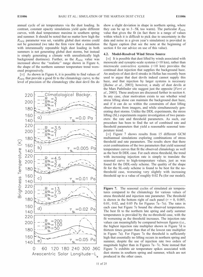
[34] It is possible that dust lifted by winds associated withmesoscale and synoptic-scale systems (>10 km), rather thanmicroscale convective systems (<10 km) provides thecontinual dust injection that supplies the background haze.An analysis of dust devil streaks in Hellas has recently beenused to argue that dust devils indeed cannot supply thishaze, and that injection by larger systems is necessary[Balme et al., 2003]; however, a study of dust devils atthe Mars Pathfinder site suggest just the opposite [Ferri etal., 2003]. These analyses are discussed further in section 6.In any case, clear motivation exists to see whether windstress lifting alone can maintain the background dust haze,and if it can do so within the constraints of dust liftingobservations from imagers, and while simultaneously gen-erating dust storms. Unlike the DDL experiments, the stresslifting (SL) experiments require investigation of two param-eters: the rate and threshold parameters. As such, ourprocedure has been to find the set of combined rate andthreshold parameters that yield a reasonable seasonal tem-perature trend.[35] Figure 7 shows results from 15 different GCM

multiannual simulations exploring combinations of stressthreshold and rate parameters. The results show that thereexist combinations of the two parameters that yield seasonaltemperature curves that fit the observed climatology as wellas the best fit DDL case. For each stress threshold, the trendwith increasing injection rate is simply to translate theseasonal curve to high-temperature values, just as wasfound for the DDL-only scheme. The quality of the shapefit for the SL-only scheme is found to be best for the no-threshold case, worsening very slightly with increasingthreshold up to a value of roughly 0.02 Pa (for our model).

Figure 7. The seasonal cycles of simulated air tempera-tures compared to the climatology for various values ofstress threshold and injection rate parameter. The thresholdis shown in the bottom right of each panel (t = 0, 0.005,0.01, 0.02, and 0.05 Pa for Figures 7a–7e). The rates ineach case but Figure 7e bound the observed temperatures.The best fit to the northern late spring and early summertemperatures is provided by the no-threshold case, with thefit worsening as the threshold increases. The injection ratevalues can meaningfully be compared between figures (i.e.,the highest injection rate multiplier shown in Figure 7d isthirteen times greater than that of the lowest rate multiplierin Figure 7a). For Figure 7e the threshold is sufficientlyhigh that essentially no lifting occurs in northern spring andsummer, despite the use of injection rate two orders ofmagnitude higher than in Figures 7a–7c. Note instead thatFigure 7e exhibits air temperature spikes associated withdust storms in southern spring and summer, which are notproduced in the other cases.


11 of 25

E11006

By the time a threshold of 0.05 Pa is reached, no amount ofdust injection will allow the model to fit the observations. Inthis case, the threshold is too high for the surface winds toactivate dust lifting. The temperature curves for the periodsbetween Ls = 60� and Ls = 180� for this threshold corre-spond to that of a completely dust free atmosphere.[36] The effect of increasing the threshold is to decrease

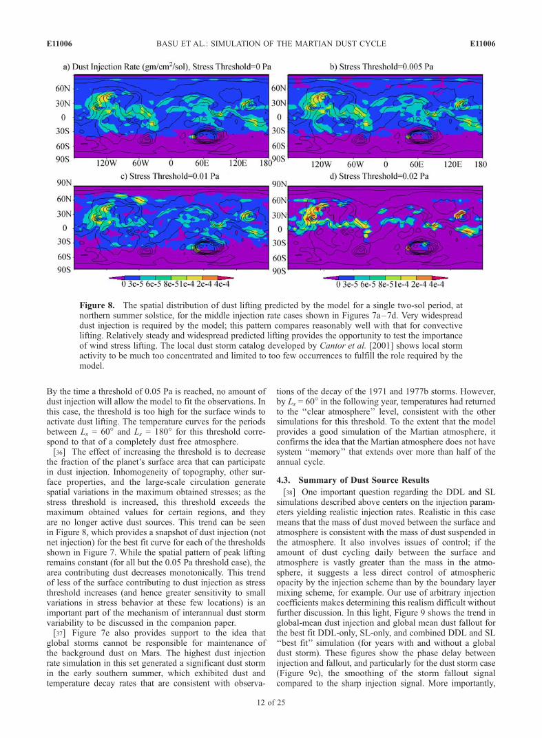
the fraction of the planet’s surface area that can participatein dust injection. Inhomogeneity of topography, other sur-face properties, and the large-scale circulation generatespatial variations in the maximum obtained stresses; as thestress threshold is increased, this threshold exceeds themaximum obtained values for certain regions, and theyare no longer active dust sources. This trend can be seenin Figure 8, which provides a snapshot of dust injection (notnet injection) for the best fit curve for each of the thresholdsshown in Figure 7. While the spatial pattern of peak liftingremains constant (for all but the 0.05 Pa threshold case), thearea contributing dust decreases monotonically. This trendof less of the surface contributing to dust injection as stressthreshold increases (and hence greater sensitivity to smallvariations in stress behavior at these few locations) is animportant part of the mechanism of interannual dust stormvariability to be discussed in the companion paper.[37] Figure 7e also provides support to the idea that

global storms cannot be responsible for maintenance ofthe background dust on Mars. The highest dust injectionrate simulation in this set generated a significant dust stormin the early southern summer, which exhibited dust andtemperature decay rates that are consistent with observa-

tions of the decay of the 1971 and 1977b storms. However,by Ls = 60� in the following year, temperatures had returnedto the ‘‘clear atmosphere’’ level, consistent with the othersimulations for this threshold. To the extent that the modelprovides a good simulation of the Martian atmosphere, itconfirms the idea that the Martian atmosphere does not havesystem ‘‘memory’’ that extends over more than half of theannual cycle.

4.3. Summary of Dust Source Results

[38] One important question regarding the DDL and SLsimulations described above centers on the injection param-eters yielding realistic injection rates. Realistic in this casemeans that the mass of dust moved between the surface andatmosphere is consistent with the mass of dust suspended inthe atmosphere. It also involves issues of control; if theamount of dust cycling daily between the surface andatmosphere is vastly greater than the mass in the atmo-sphere, it suggests a less direct control of atmosphericopacity by the injection scheme than by the boundary layermixing scheme, for example. Our use of arbitrary injectioncoefficients makes determining this realism difficult withoutfurther discussion. In this light, Figure 9 shows the trend inglobal-mean dust injection and global mean dust fallout forthe best fit DDL-only, SL-only, and combined DDL and SL‘‘best fit’’ simulation (for years with and without a globaldust storm). These figures show the phase delay betweeninjection and fallout, and particularly for the dust storm case(Figure 9c), the smoothing of the storm fallout signalcompared to the sharp injection signal. More importantly,

Figure 8. The spatial distribution of dust lifting predicted by the model for a single two-sol period, atnorthern summer solstice, for the middle injection rate cases shown in Figures 7a–7d. Very widespreaddust injection is required by the model; this pattern compares reasonably well with that for convectivelifting. Relatively steady and widespread predicted lifting provides the opportunity to test the importanceof wind stress lifting. The local dust storm catalog developed by Cantor et al. [2001] shows local stormactivity to be much too concentrated and limited to too few occurrences to fulfill the role required by themodel.


12 of 25

E11006

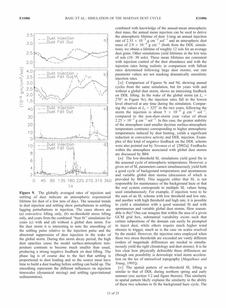
combined with knowledge of the annual-mean atmosphericdust mass, the annual mean injection can be used to derivethe atmospheric lifetime of dust. Using an annual injectionrate of 2.35 � 10�5 g cm�2 sol�1 and an atmospheric dustmass of 2.9 � 10�4 g cm�2 (both from the DDL simula-tion), we obtain a lifetime of roughly 12 sols for an averagedust grain. Other simulations yield lifetimes in the low tensof sols (10–30 sols). These mean lifetimes are consistentwith injection control of the dust abundance and with theinjection rates being realistic in comparison with falloutrates determined following large dust storms; our rateparameter values are not masking dramatically unrealisticinjection rates.[39] Comparison of Figures 9c and 9d, showing annual

cycles from the same simulation, but for years with andwithout a global dust storm, shows an interesting feedbackon DDL lifting. In the wake of the global storm (at Ls =270� in Figure 9c), the injection rates fall to the lowestlevel observed at any time during the simulation. Compar-ing the values at Ls = 325� in the two years, following thestorm the injection is about 5 � 10�6 g cm�2 sol�1,compared to the non-dust-storm year value of about2.25 � 10�5 g cm�2 sol�1. In this case, the greater stabilityof the atmosphere (and smaller daytime surface-atmospheretemperature contrasts) corresponding to higher atmospherictemperatures induced by dust heating, yields a significantreduction in convective activity and DDL injection. Exam-ples of this kind of negative feedback on the DDL schemewere also pointed out by Newman et al. [2002a]. Feedbackswithin the atmosphere associated with global dust stormsare discussed by B04.[40] The low-threshold SL simulations yield good fits to

the seasonal cycle of atmospheric temperatures. However, agiven set of SL parameters cannot simultaneously yield botha good cycle of background temperatures and spontaneousand variable global dust storms (discussion of which isprovided by B04). This suggests either that SL is notresponsible for maintenance of the background haze or thatthe real system corresponds to multiple SL values beingused simultaneously. For example, if injection were to bethe sum of an SL scheme with low threshold and low rate,and another with high threshold and high rate, it is possibleto yield a simulation with a good seasonal fit and withspontaneous and variable global dust storms. How reason-able is this? One can imagine that within the area of a givenGCM grid box, substantial variability exists such thatcertain subportions of the domain can easily be promptedto inject dust, while others require much higher windstresses to trigger, much as is the case on scales resolvedby the model. However, the injection rates employed whenthese two stress thresholds are exceeded are vastly different(orders of magnitude differences are needed to simulta-neously yield the right climatology and dust storms). It is farless clear how physically defensible these differences are(though one possibility is downslope wind storm accelera-tion on the lee of unresolved topography [Magalhaes andYoung, 1995]).[41] The spatial pattern of no-threshold SL lifting is

similar to that of DDL during northern spring and earlysummer (see section 5.2 and figure therein). This similarityin spatial pattern likely explains the similarity in the abilityof these two schemes to fit the background haze cycle. The

Figure 9. The globally averaged rates of injection andsettling of dust indicate an atmospheric exponentiallifetime for dust of a few tens of days. The seasonal trendsin dust injection and settling show perturbations in settlinglagging perturbations in injection. The cases shown are(a) convective lifting only, (b) no-threshold stress liftingonly, and years from the combined ‘‘best fit’’ simulations foryears (c) with and (d) without a global dust storm. Forthe dust storm it is interesting to note the smoothing ofthe settling pulse relative to the injection pulse and theabnormal suppression of dust injection in the wake ofthe global storm. During this storm decay period, the highdust opacities cause the model surface-atmosphere tem-perature contrasts to become much smaller than usual,producing a strong negative feedback on dust lifting. Thephase lag is of course due to the fact that settling isproportional to dust loading and so the source must havetime to build a dust loading before settling can build up. Thesmoothing represents the different influences on injectiontimescales (dynamical mixing) and settling (gravitationalsedimentation).


13 of 25

E11006

dominant control of this pattern for DDL is clearly associ-ated with the spatial variation of thermal convective vigor,as discussed in section 3.1. That the no-threshold case SLand DDL produce a very similar spatial pattern suggests thata major control on the injection, via the imparted windstress, is through the variation of the drag parameterassociated with variations in the vigor of convective activityduring the day. This similarity does not argue for oneinjection process over the other, but suggests instead thatthe controlling physical processes might not be as distinct inthe two schemes as one might expect at first glance.[42] Discrimination between DDL and SL roles in the

maintenance of background haze most likely can be madeon the basis of observations. The DDL scheme predictswidespread and ongoing dust devil activity, and particularseasonal variation of injection. Images of Mars from orbitand from landers show abundant dust devil activity in theform of dust devils and dust devil tracks across the planet[Metzger et al., 1999;Malin and Edgett, 2001; Cantor et al.,2002; Fisher et al., 2002; Balme et al., 2003; Ferri et al.,2003]. As shown at the end of section 5.2, the modelpredictions of dust injection during northern summer agreesremarkably well with the estimates of dust devil lifting fromImager for Mars Pathfinder data analysis [Ferri et al.,2003].[43] The model also predicts that if low- or no-threshold

SL controls the background haze, widespread and continu-ously ongoing non-dust-devil lifting should be active.Figure 8 shows low-threshold injection averaged over 2sols, requiring dust lifting within each grid box over a verylarge fraction of the planet’s surface. However, in theexhaustive survey of local dust storms described by Cantoret al. [2001], for the period near Ls = 110�, on any givenday, only two or three storms with areas over 103 km2 werecounted over the entire planet. This is a vastly smaller areaof dust lifting than that predicted by the no-threshold SLcase, and more in keeping with the very much higherthreshold SL cases required to generate large storms.Systems smaller than about 100 km2 cannot be observedin the MOC daily global map images, but are very rarelyeven seen in the MOC narrow angle images (at 1–10 mresolution), which would seem to be inconsistent with thewidespread, regular lifting predicted by the no-threshold SLsimulation (the low resolution of the daily global mapimages also precludes the use of this data to capture thetotal number of dust devils occurring on a given day belowthe spacecraft track).[44] Other types of dust lifting, apart from dust devils and

local storms are possible. Dust streaks are evident on thesurface associated with craters and other forms of sharptopography [Thomas et al., 1981, 1984], and the highstresses in the lee of these objects might be important(obviously it is only dark, erosional wind streaks that areof interest as potential sources of dust). One factor arguingagainst the role of lee stresses is frequency of activity:fitting of wind directions to observed streaks suggest thatthey form rapidly by eroding nonequilibrium dust deposits(such as those deposited following a large dust storm) atspecific times of day when the stresses are highest [Fentonand Richardson, 2001; Thomas et al., 2003]. However,lifting can only be sustained until these very limited areasare depleted (yielding the dark streak). We are therefore

dubious of the role of such lifting, but this is a bias thatrequires a focused study before conclusions can be drawn.Finally, it is possible that some microscale lifting process isat work that is below the resolution of orbiting cameras, butis also never seen in lander images. To determine if such‘‘stealth’’ lifting is ongoing to the degree required by the SLscheme, it may be necessary to measure the net vertical fluxof dust on future landers.[45] In summary, the observed lack of dust motion at the

Viking Lander sites except during extreme wind events[Moore, 1985], and the only observation of dust lifting atthe Pathfinder site being associated with dust devils[Metzger et al., 1999], also argue that nonconvective liftingof dust is rare at most locations on Mars. Local dust stormsare insufficiently active, based on comparison with theCantor et al. [2001] catalog. Given the abundant evidencefor dust devils across the surface, and the lack of observa-tions of an adequate non-dust-devil lifting mechanism, itseems that the dust devil lifting mechanism is the mostplausible. This interpretation is further supported by theease with which the annual cycle can be fit with a combi-nation of DDL and high-threshold SL, but that a combina-tion of high and low SL is needed if DDL does notdominate the haze maintenance, and that these two SLmodes require orders-of-magnitude different injection rateparameters. Plausibility would currently seem to us tostrongly support a dominant role for dust devils in themaintenance of the background haze. However, furtherobservational study is needed before this opinion can beestablished as a fact.

5. Characteristics of the ‘‘Best Fit’’ ModelAnnual Cycle

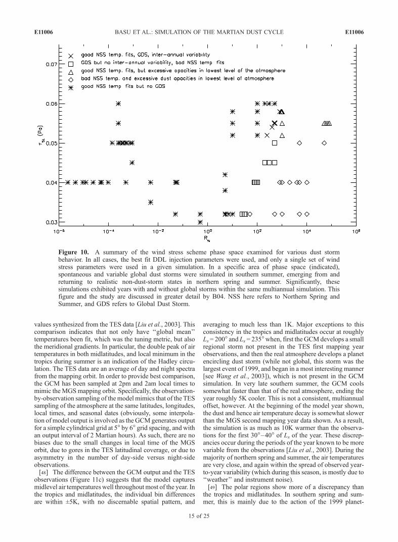
[46] Examination of the model seasonal cycles describedin section 4 and associated arguments can lead to aparadigm for a ‘‘best fit’’ model climate in which DDLlifting provides control of the seasonal haze cycle andSL control of dust storms. In this way, a ‘‘best fit’’ annualcycle simulation can be found by varying the RDDL untilthe background seasonal air temperature cycle is fit(with emphasis on northern spring and summer), and thenvarying the RSL and tSL values until variable dust stormsare generated in southern spring and summer. A very largeamount of phase space was examined, as shown inFigure 10. This figure summarizes the dust storm simula-tions (all using the same DDL parameters), categorizingthem on the basis of whether they yielded realistic non-dust-storm climates and the nature of the dust storm activitygenerated. An area of phase space was found in whichspontaneous and interannually (and intra-annually) variableglobal dust storms were produced in southern spring andsummer, and which would relax back to a realistic thermalstate after these events. Output from such a ‘‘best fit’’ case isdescribed in this section. The dust storms generated by thissimulation are described in some detail by B04.

5.1. Meridional and Vertical Distribution of AirTemperature

[47] For a year without a major dust storm, Figure 11shows the comparison of the seasonal cycle of meridionalmidlevel air temperatures with observations (IRTM T15


14 of 25

E11006

values synthesized from the TES data [Liu et al., 2003]. Thiscomparison indicates that not only have ‘‘global mean’’temperatures been fit, which was the tuning metric, but alsothe meridional gradients. In particular, the double peak of airtemperatures in both midlatitudes, and local minimum in thetropics during summer is an indication of the Hadley circu-lation. The TES data are an average of day and night spectrafrom the mapping orbit. In order to provide best comparison,the GCM has been sampled at 2pm and 2am local times tomimic the MGSmapping orbit. Specifically, the observation-by-observation sampling of the model mimics that of the TESsampling of the atmosphere at the same latitudes, longitudes,local times, and seasonal dates (obviously, some interpola-tion of model output is involved as the GCMgenerates outputfor a simple cylindrical grid at 5� by 6� grid spacing, and withan output interval of 2 Martian hours). As such, there are nobiases due to the small changes in local time of the MGSorbit, due to gores in the TES latitudinal coverage, or due toasymmetry in the number of day-side versus night-sideobservations.[48] The difference between the GCM output and the TES

observations (Figure 11c) suggests that the model capturesmidlevel air temperatures well throughout most of the year. Inthe tropics and midlatitudes, the individual bin differencesare within ±5K, with no discernable spatial pattern, and

averaging to much less than 1K. Major exceptions to thisconsistency in the tropics and midlatitudes occur at roughlyLs = 200� and Ls = 235�when, first the GCMdevelops a smallregional storm not present in the TES first mapping yearobservations, and then the real atmosphere develops a planetencircling dust storm (while not global, this storm was thelargest event of 1999, and began in a most interesting manner[see Wang et al., 2003]), which is not present in the GCMsimulation. In very late southern summer, the GCM coolssomewhat faster than that of the real atmosphere, ending theyear roughly 5K cooler. This is not a consistent, multiannualoffset, however. At the beginning of the model year shown,the dust and hence air temperature decay is somewhat slowerthan the MGS second mapping year data shown. As a result,the simulation is as much as 10K warmer than the observa-tions for the first 30�–40� of Ls of the year. These discrep-ancies occur during the periods of the year known to be morevariable from the observations [Liu et al., 2003]. During themajority of northern spring and summer, the air temperaturesare very close, and again within the spread of observed year-to-year variability (which during this season, is mostly due to‘‘weather’’ and instrument noise).[49] The polar regions show more of a discrepancy than

the tropics and midlatitudes. In southern spring and sum-mer, this is mainly due to the action of the 1999 planet-

Figure 10. A summary of the wind stress scheme phase space examined for various dust stormbehavior. In all cases, the best fit DDL injection parameters were used, and only a single set of windstress parameters were used in a given simulation. In a specific area of phase space (indicated),spontaneous and variable global dust storms were simulated in southern summer, emerging from andreturning to realistic non-dust-storm states in northern spring and summer. Significantly, thesesimulations exhibited years with and without global storms within the same multiannual simulation. Thisfigure and the study are discussed in greater detail by B04. NSS here refers to Northern Spring andSummer, and GDS refers to Global Dust Storm.


15 of 25

E11006

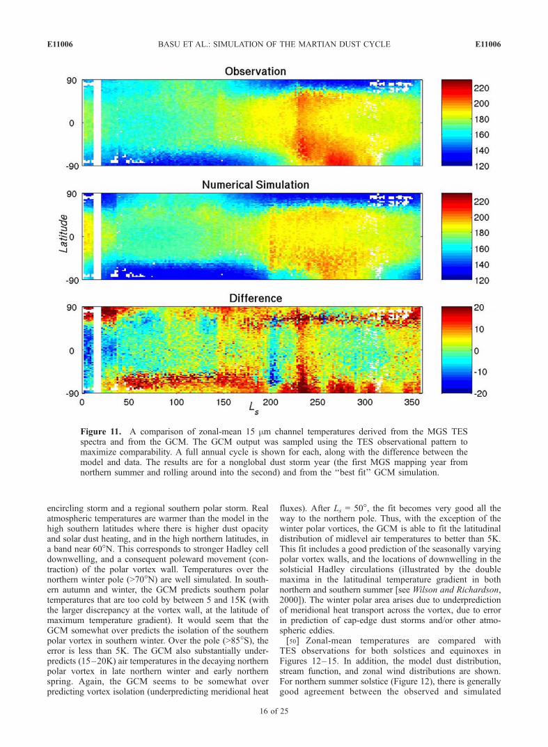
encircling storm and a regional southern polar storm. Realatmospheric temperatures are warmer than the model in thehigh southern latitudes where there is higher dust opacityand solar dust heating, and in the high northern latitudes, ina band near 60�N. This corresponds to stronger Hadley celldownwelling, and a consequent poleward movement (con-traction) of the polar vortex wall. Temperatures over thenorthern winter pole (>70�N) are well simulated. In south-ern autumn and winter, the GCM predicts southern polartemperatures that are too cold by between 5 and 15K (withthe larger discrepancy at the vortex wall, at the latitude ofmaximum temperature gradient). It would seem that theGCM somewhat over predicts the isolation of the southernpolar vortex in southern winter. Over the pole (>85�S), theerror is less than 5K. The GCM also substantially under-predicts (15–20K) air temperatures in the decaying northernpolar vortex in late northern winter and early northernspring. Again, the GCM seems to be somewhat overpredicting vortex isolation (underpredicting meridional heat

fluxes). After Ls = 50�, the fit becomes very good all theway to the northern pole. Thus, with the exception of thewinter polar vortices, the GCM is able to fit the latitudinaldistribution of midlevel air temperatures to better than 5K.This fit includes a good prediction of the seasonally varyingpolar vortex walls, and the locations of downwelling in thesolsticial Hadley circulations (illustrated by the doublemaxima in the latitudinal temperature gradient in bothnorthern and southern summer [see Wilson and Richardson,2000]). The winter polar area arises due to underpredictionof meridional heat transport across the vortex, due to errorin prediction of cap-edge dust storms and/or other atmo-spheric eddies.[50] Zonal-mean temperatures are compared with

TES observations for both solstices and equinoxes inFigures 12–15. In addition, the model dust distribution,stream function, and zonal wind distributions are shown.For northern summer solstice (Figure 12), there is generallygood agreement between the observed and simulated

Figure 11. A comparison of zonal-mean 15 mm channel temperatures derived from the MGS TESspectra and from the GCM. The GCM output was sampled using the TES observational pattern tomaximize comparability. A full annual cycle is shown for each, along with the difference between themodel and data. The results are for a nonglobal dust storm year (the first MGS mapping year fromnorthern summer and rolling around into the second) and from the ‘‘best fit’’ GCM simulation.


16 of 25

E11006

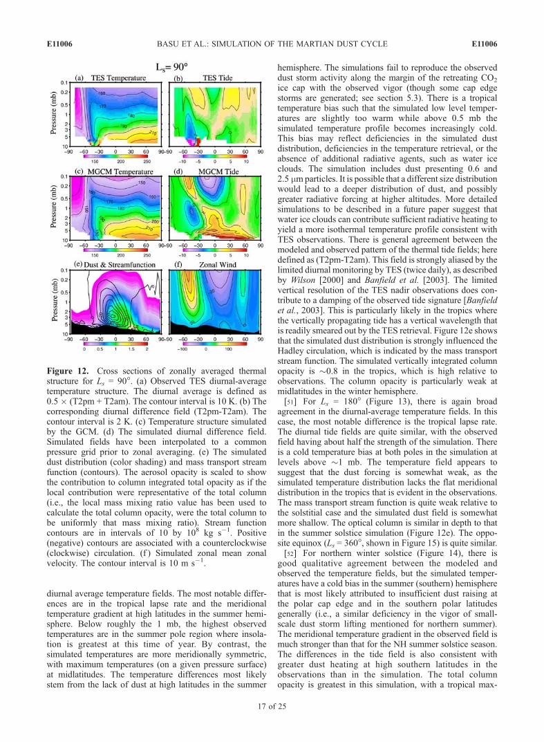
diurnal average temperature fields. The most notable differ-ences are in the tropical lapse rate and the meridionaltemperature gradient at high latitudes in the summer hemi-sphere. Below roughly the 1 mb, the highest observedtemperatures are in the summer pole region where insola-tion is greatest at this time of year. By contrast, thesimulated temperatures are more meridionally symmetric,with maximum temperatures (on a given pressure surface)at midlatitudes. The temperature differences most likelystem from the lack of dust at high latitudes in the summer

hemisphere. The simulations fail to reproduce the observeddust storm activity along the margin of the retreating CO2

ice cap with the observed vigor (though some cap edgestorms are generated; see section 5.3). There is a tropicaltemperature bias such that the simulated low level temper-atures are slightly too warm while above 0.5 mb thesimulated temperature profile becomes increasingly cold.This bias may reflect deficiencies in the simulated dustdistribution, deficiencies in the temperature retrieval, or theabsence of additional radiative agents, such as water iceclouds. The simulation includes dust presenting 0.6 and2.5 mmparticles. It is possible that a different size distributionwould lead to a deeper distribution of dust, and possiblygreater radiative forcing at higher altitudes. More detailedsimulations to be described in a future paper suggest thatwater ice clouds can contribute sufficient radiative heating toyield a more isothermal temperature profile consistent withTES observations. There is general agreement between themodeled and observed pattern of the thermal tide fields; heredefined as (T2pm-T2am). This field is strongly aliased by thelimited diurnal monitoring by TES (twice daily), as describedby Wilson [2000] and Banfield et al. [2003]. The limitedvertical resolution of the TES nadir observations does con-tribute to a damping of the observed tide signature [Banfieldet al., 2003]. This is particularly likely in the tropics wherethe vertically propagating tide has a vertical wavelength thatis readily smeared out by the TES retrieval. Figure 12e showsthat the simulated dust distribution is strongly influenced theHadley circulation, which is indicated by the mass transportstream function. The simulated vertically integrated columnopacity is �0.8 in the tropics, which is high relative toobservations. The column opacity is particularly weak atmidlatitudes in the winter hemisphere.[51] For Ls = 180� (Figure 13), there is again broad

agreement in the diurnal-average temperature fields. In thiscase, the most notable difference is the tropical lapse rate.The diurnal tide fields are quite similar, with the observedfield having about half the strength of the simulation. Thereis a cold temperature bias at both poles in the simulation atlevels above �1 mb. The temperature field appears tosuggest that the dust forcing is somewhat weak, as thesimulated temperature distribution lacks the flat meridionaldistribution in the tropics that is evident in the observations.The mass transport stream function is quite weak relative tothe solstitial case and the simulated dust field is somewhatmore shallow. The optical column is similar in depth to thatin the summer solstice simulation (Figure 12e). The oppo-site equinox (Ls = 360�, shown in Figure 15) is quite similar.[52] For northern winter solstice (Figure 14), there is

good qualitative agreement between the modeled andobserved the temperature fields, but the simulated temper-atures have a cold bias in the summer (southern) hemispherethat is most likely attributed to insufficient dust raising atthe polar cap edge and in the southern polar latitudesgenerally (i.e., a similar deficiency in the vigor of small-scale dust storm lifting mentioned for northern summer).The meridional temperature gradient in the observed field ismuch stronger than that for the NH summer solstice season.The differences in the tide field is also consistent withgreater dust heating at high southern latitudes in theobservations than in the simulation. The total columnopacity is greatest in this simulation, with a tropical max-

Figure 12. Cross sections of zonally averaged thermalstructure for Ls = 90�. (a) Observed TES diurnal-averagetemperature structure. The diurnal average is defined as0.5 � (T2pm + T2am). The contour interval is 10 K. (b) Thecorresponding diurnal difference field (T2pm-T2am). Thecontour interval is 2 K. (c) Temperature structure simulatedby the GCM. (d) The simulated diurnal difference field.Simulated fields have been interpolated to a commonpressure grid prior to zonal averaging. (e) The simulateddust distribution (color shading) and mass transport streamfunction (contours). The aerosol opacity is scaled to showthe contribution to column integrated total opacity as if thelocal contribution were representative of the total column(i.e., the local mass mixing ratio value has been used tocalculate the total column opacity, were the total column tobe uniformly that mass mixing ratio). Stream functioncontours are in intervals of 10 by 108 kg s�1. Positive(negative) contours are associated with a counterclockwise(clockwise) circulation. (f ) Simulated zonal mean zonalvelocity. The contour interval is 10 m s�1.


17 of 25

E11006

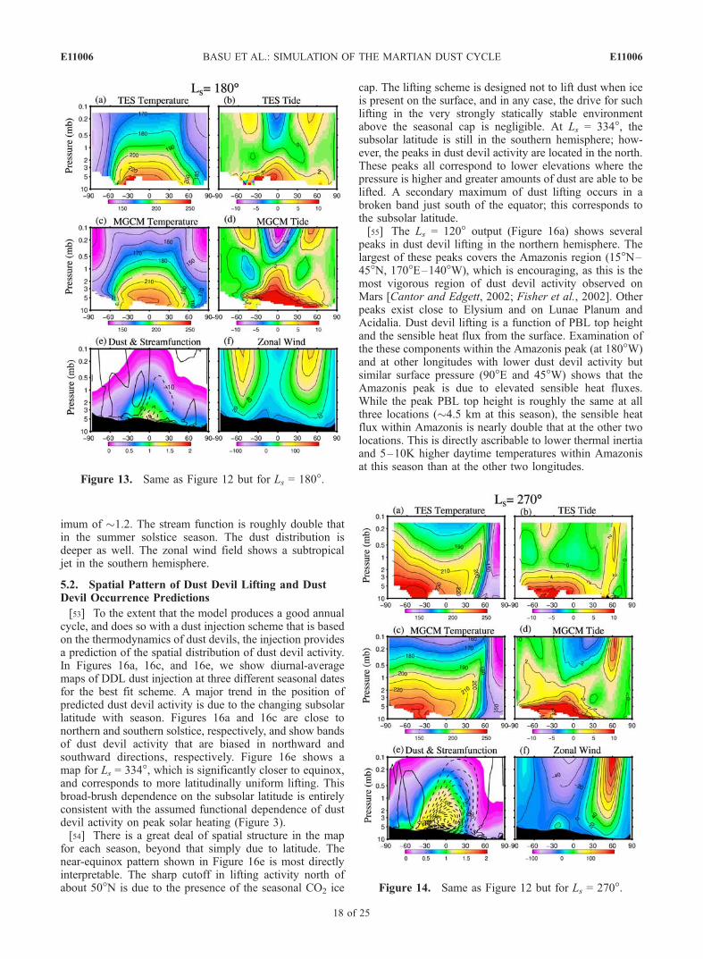
imum of �1.2. The stream function is roughly double thatin the summer solstice season. The dust distribution isdeeper as well. The zonal wind field shows a subtropicaljet in the southern hemisphere.

5.2. Spatial Pattern of Dust Devil Lifting and DustDevil Occurrence Predictions

[53] To the extent that the model produces a good annualcycle, and does so with a dust injection scheme that is basedon the thermodynamics of dust devils, the injection providesa prediction of the spatial distribution of dust devil activity.In Figures 16a, 16c, and 16e, we show diurnal-averagemaps of DDL dust injection at three different seasonal datesfor the best fit scheme. A major trend in the position ofpredicted dust devil activity is due to the changing subsolarlatitude with season. Figures 16a and 16c are close tonorthern and southern solstice, respectively, and show bandsof dust devil activity that are biased in northward andsouthward directions, respectively. Figure 16e shows amap for Ls = 334�, which is significantly closer to equinox,and corresponds to more latitudinally uniform lifting. Thisbroad-brush dependence on the subsolar latitude is entirelyconsistent with the assumed functional dependence of dustdevil activity on peak solar heating (Figure 3).[54] There is a great deal of spatial structure in the map

for each season, beyond that simply due to latitude. Thenear-equinox pattern shown in Figure 16e is most directlyinterpretable. The sharp cutoff in lifting activity north ofabout 50�N is due to the presence of the seasonal CO2 ice

cap. The lifting scheme is designed not to lift dust when iceis present on the surface, and in any case, the drive for suchlifting in the very strongly statically stable environmentabove the seasonal cap is negligible. At Ls = 334�, thesubsolar latitude is still in the southern hemisphere; how-ever, the peaks in dust devil activity are located in the north.These peaks all correspond to lower elevations where thepressure is higher and greater amounts of dust are able to belifted. A secondary maximum of dust lifting occurs in abroken band just south of the equator; this corresponds tothe subsolar latitude.[55] The Ls = 120� output (Figure 16a) shows several

peaks in dust devil lifting in the northern hemisphere. Thelargest of these peaks covers the Amazonis region (15�N–45�N, 170�E–140�W), which is encouraging, as this is themost vigorous region of dust devil activity observed onMars [Cantor and Edgett, 2002; Fisher et al., 2002]. Otherpeaks exist close to Elysium and on Lunae Planum andAcidalia. Dust devil lifting is a function of PBL top heightand the sensible heat flux from the surface. Examination ofthe these components within the Amazonis peak (at 180�W)and at other longitudes with lower dust devil activity butsimilar surface pressure (90�E and 45�W) shows that theAmazonis peak is due to elevated sensible heat fluxes.While the peak PBL top height is roughly the same at allthree locations (�4.5 km at this season), the sensible heatflux within Amazonis is nearly double that at the other twolocations. This is directly ascribable to lower thermal inertiaand 5–10K higher daytime temperatures within Amazonisat this season than at the other two longitudes.

Figure 13. Same as Figure 12 but for Ls = 180�.



18 of 25

E11006

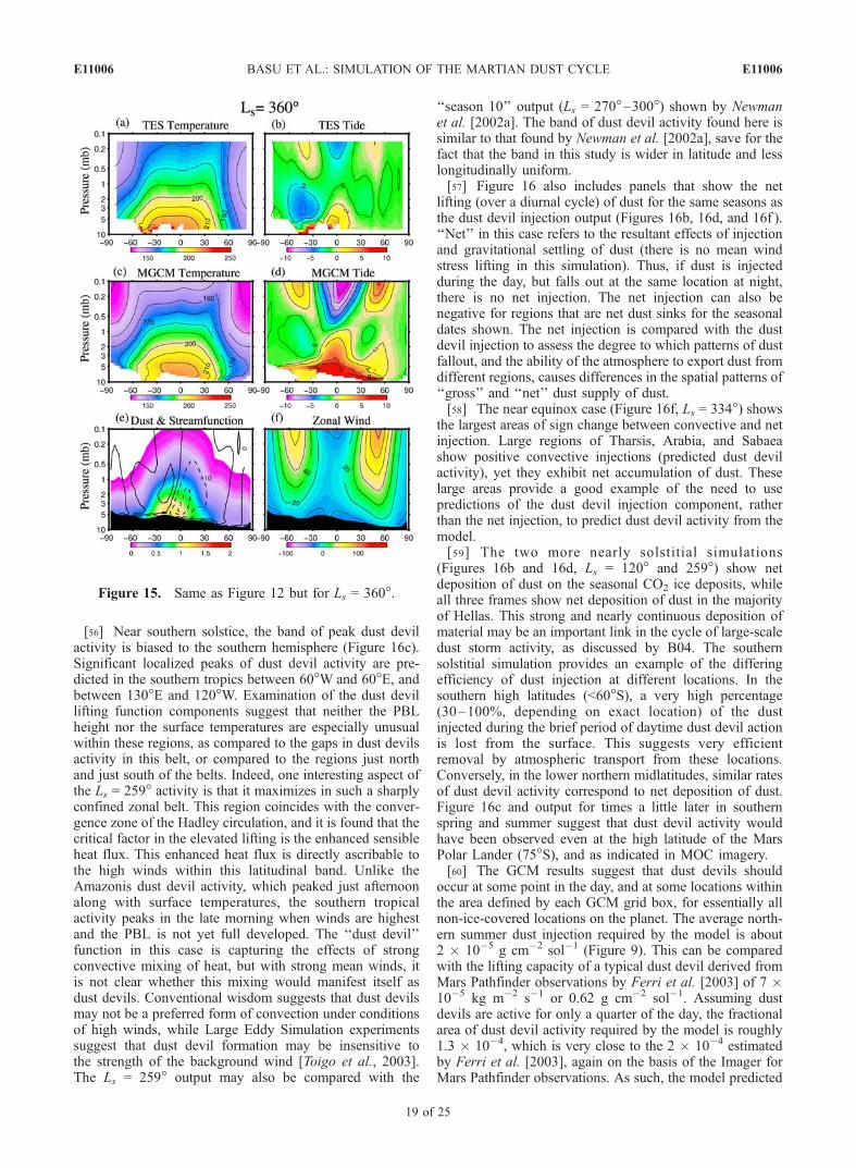
[56] Near southern solstice, the band of peak dust devilactivity is biased to the southern hemisphere (Figure 16c).Significant localized peaks of dust devil activity are pre-dicted in the southern tropics between 60�W and 60�E, andbetween 130�E and 120�W. Examination of the dust devillifting function components suggest that neither the PBLheight nor the surface temperatures are especially unusualwithin these regions, as compared to the gaps in dust devilsactivity in this belt, or compared to the regions just northand just south of the belts. Indeed, one interesting aspect ofthe Ls = 259� activity is that it maximizes in such a sharplyconfined zonal belt. This region coincides with the conver-gence zone of the Hadley circulation, and it is found that thecritical factor in the elevated lifting is the enhanced sensibleheat flux. This enhanced heat flux is directly ascribable tothe high winds within this latitudinal band. Unlike theAmazonis dust devil activity, which peaked just afternoonalong with surface temperatures, the southern tropicalactivity peaks in the late morning when winds are highestand the PBL is not yet full developed. The ‘‘dust devil’’function in this case is capturing the effects of strongconvective mixing of heat, but with strong mean winds, itis not clear whether this mixing would manifest itself asdust devils. Conventional wisdom suggests that dust devilsmay not be a preferred form of convection under conditionsof high winds, while Large Eddy Simulation experimentssuggest that dust devil formation may be insensitive tothe strength of the background wind [Toigo et al., 2003].The Ls = 259� output may also be compared with the

‘‘season 10’’ output (Ls = 270�–300�) shown by Newmanet al. [2002a]. The band of dust devil activity found here issimilar to that found by Newman et al. [2002a], save for thefact that the band in this study is wider in latitude and lesslongitudinally uniform.[57] Figure 16 also includes panels that show the net

lifting (over a diurnal cycle) of dust for the same seasons asthe dust devil injection output (Figures 16b, 16d, and 16f ).‘‘Net’’ in this case refers to the resultant effects of injectionand gravitational settling of dust (there is no mean windstress lifting in this simulation). Thus, if dust is injectedduring the day, but falls out at the same location at night,there is no net injection. The net injection can also benegative for regions that are net dust sinks for the seasonaldates shown. The net injection is compared with the dustdevil injection to assess the degree to which patterns of dustfallout, and the ability of the atmosphere to export dust fromdifferent regions, causes differences in the spatial patterns of‘‘gross’’ and ‘‘net’’ dust supply of dust.[58] The near equinox case (Figure 16f, Ls = 334�) shows

the largest areas of sign change between convective and netinjection. Large regions of Tharsis, Arabia, and Sabaeashow positive convective injections (predicted dust devilactivity), yet they exhibit net accumulation of dust. Theselarge areas provide a good example of the need to usepredictions of the dust devil injection component, ratherthan the net injection, to predict dust devil activity from themodel.[59] The two more nearly solstitial simulations

(Figures 16b and 16d, Ls = 120� and 259�) show netdeposition of dust on the seasonal CO2 ice deposits, whileall three frames show net deposition of dust in the majorityof Hellas. This strong and nearly continuous deposition ofmaterial may be an important link in the cycle of large-scaledust storm activity, as discussed by B04. The southernsolstitial simulation provides an example of the differingefficiency of dust injection at different locations. In thesouthern high latitudes (<60�S), a very high percentage(30–100%, depending on exact location) of the dustinjected during the brief period of daytime dust devil actionis lost from the surface. This suggests very efficientremoval by atmospheric transport from these locations.Conversely, in the lower northern midlatitudes, similar ratesof dust devil activity correspond to net deposition of dust.Figure 16c and output for times a little later in southernspring and summer suggest that dust devil activity wouldhave been observed even at the high latitude of the MarsPolar Lander (75�S), and as indicated in MOC imagery.[60] The GCM results suggest that dust devils should

occur at some point in the day, and at some locations withinthe area defined by each GCM grid box, for essentially allnon-ice-covered locations on the planet. The average north-ern summer dust injection required by the model is about2 � 10�5 g cm�2 sol�1 (Figure 9). This can be comparedwith the lifting capacity of a typical dust devil derived fromMars Pathfinder observations by Ferri et al. [2003] of 7 �10�5 kg m�2 s�1 or 0.62 g cm�2 sol�1. Assuming dustdevils are active for only a quarter of the day, the fractionalarea of dust devil activity required by the model is roughly1.3 � 10�4, which is very close to the 2 � 10�4 estimatedby Ferri et al. [2003], again on the basis of the Imager forMars Pathfinder observations. As such, the model predicted



19 of 25

E11006

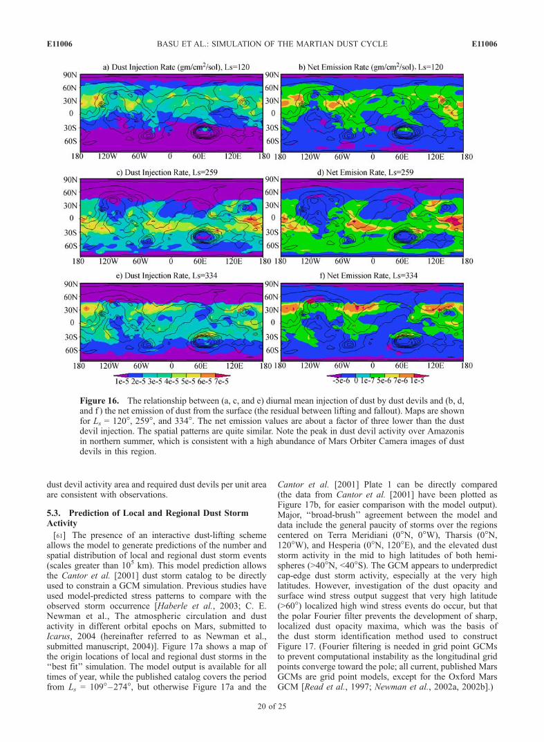
dust devil activity area and required dust devils per unit areaare consistent with observations.

5.3. Prediction of Local and Regional Dust StormActivity

[61] The presence of an interactive dust-lifting schemeallows the model to generate predictions of the number andspatial distribution of local and regional dust storm events(scales greater than 105 km). This model prediction allowsthe Cantor et al. [2001] dust storm catalog to be directlyused to constrain a GCM simulation. Previous studies haveused model-predicted stress patterns to compare with theobserved storm occurrence [Haberle et al., 2003; C. E.Newman et al., The atmospheric circulation and dustactivity in different orbital epochs on Mars, submitted toIcarus, 2004 (hereinafter referred to as Newman et al.,submitted manuscript, 2004)]. Figure 17a shows a map ofthe origin locations of local and regional dust storms in the‘‘best fit’’ simulation. The model output is available for alltimes of year, while the published catalog covers the periodfrom Ls = 109�–274�, but otherwise Figure 17a and the

Cantor et al. [2001] Plate 1 can be directly compared(the data from Cantor et al. [2001] have been plotted asFigure 17b, for easier comparison with the model output).Major, ‘‘broad-brush’’ agreement between the model anddata include the general paucity of storms over the regionscentered on Terra Meridiani (0�N, 0�W), Tharsis (0�N,120�W), and Hesperia (0�N, 120�E), and the elevated duststorm activity in the mid to high latitudes of both hemi-spheres (>40�N, <40�S). The GCM appears to underpredictcap-edge dust storm activity, especially at the very highlatitudes. However, investigation of the dust opacity andsurface wind stress output suggest that very high latitude(>60�) localized high wind stress events do occur, but thatthe polar Fourier filter prevents the development of sharp,localized dust opacity maxima, which was the basis ofthe dust storm identification method used to constructFigure 17. (Fourier filtering is needed in grid point GCMsto prevent computational instability as the longitudinal gridpoints converge toward the pole; all current, published MarsGCMs are grid point models, except for the Oxford MarsGCM [Read et al., 1997; Newman et al., 2002a, 2002b].)

Figure 16. The relationship between (a, c, and e) diurnal mean injection of dust by dust devils and (b, d,and f ) the net emission of dust from the surface (the residual between lifting and fallout). Maps are shownfor Ls = 120�, 259�, and 334�. The net emission values are about a factor of three lower than the dustdevil injection. The spatial patterns are quite similar. Note the peak in dust devil activity over Amazonisin northern summer, which is consistent with a high abundance of Mars Orbiter Camera images of dustdevils in this region.


20 of 25

E11006

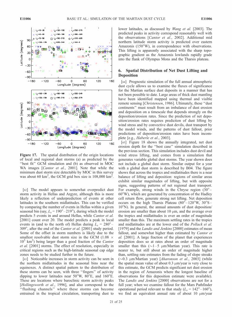
[62] The model appears to somewhat overpredict duststorm activity in Hellas and Argyre, although this is morelikely a reflection of underprediction of events at otherlatitudes in the southern midlatitudes. This can be verifiedby comparing the number of events in Hellas within a givenseasonal bin (say, Ls = 190�–219�), during which the modelpredicts 5 events in and around Hellas, while Cantor et al.[2001] count over 20. The model predicts a peak in localevents in (and to the north of) Hellas during Ls = 280�–309�, after the end of the Cantor et al. [2001] study period.Some of the offset in storm numbers is likely due to thesmallest resolvable dust storm size in the GCM (1.08 �105 km2) being larger than a good fraction of the Cantoret al. [2001] storms. The effect of resolution, especially incritical regions such as the high-latitude seasonal cap edgezones needs to be studied further in the future.[63] Noticeable increases in storm activity can be seen in

the northern midlatitudes in the seasonal bins near theequinoxes. A distinct spatial pattern to the distribution ofthese storms can be seen, with three ‘‘fingers’’ of activitydipping to lower latitudes near 50�W, 80�E, and 160�E.These are locations where baroclinic storm activity peaks[Hollingsworth et al., 1996], and also correspond to the‘‘flushing channels’’ where these storms can becomeentrained in the tropical circulation, transporting dust to

lower latitudes, as discussed by Wang et al. [2003]. Thepredicted peaks in activity correspond reasonably well withthe observations [Cantor et al., 2002]. Additional midnorthern latitude storm activity is predicted over easternAmazonis (150�W), in correspondence with observations.This lifting is apparently associated with the sharp topo-graphic gradient as the Amazonis lowlands rapidly gradeinto the flank of Olympus Mons and the Tharsis plateau.

6. Spatial Distribution of Net Dust Lifting andDeposition

[64] Prognostic simulation of the full annual atmosphericdust cycle allows us to examine the fluxes of significancefor the Martian surface dust deposits in a manner that hasnot been possible to date. Large areas of thick dust mantlinghave been identified mapped using thermal and visibleremote sensing [Christensen, 1986]. Ultimately, these ‘‘dustcontinents’’ must result from an imbalance of dust erosionand deposition on a timescale that depends strongly on thedeposition/erosion rates. Since the prediction of net depo-sition/erosion rates requires prediction of dust lifting bywind stress and by convective dust devils, dust transport bythe model winds, and the patterns of dust fallout, priorpredictions of deposition/erosion rates have been incom-plete [e.g., Haberle et al., 2003].[65] Figure 18 shows the annually integrated, net dust

erosion depth for the ‘‘best case’’ simulation described inthe previous section. This simulation includes dust devil andwind stress lifting, and comes from a simulation thatgenerates variable global dust storms. The year shown doesnot include a global dust storm. Similar output for a yearwith a global dust storm is described by B04. The figureshows that across the tropics and midlatitudes there is a nearbalance of lifting and deposition: regions of similar areasexhibit similar magnitudes of lifting, but with oppositesigns, suggesting patterns of net regional dust transport.For example, strong winds in the Chryse region (30�–60�W), which are generated by concentration of the Hadleycell return flow, generate strong net lifting. Net depositionoccurs on the high Tharsis Plateau (80�–120�W, 30�S–10�N). In general, the annual amounts of dust deposition/erosion are smaller than about 10 mm, and the average overthe tropics and midlatitudes is over an order of magnitudesmaller than this. The maximum settling rates in the tropicsand midlatitudes are at the lower end of the Pollack et al.[1979] and the Landis and Jenkins [2000] estimates of meanfallout, and somewhat higher than estimated by Cantor etal. [2001]. A large fraction of the planet that experiencesdeposition does so at rates about an order of magnitudesmaller than this (�1–5 mm/Martian year). This rate isnearer to, but still about an order of magnitude higherthan, settling rate estimates from the fading of slope streaks(�0.3 mm/Martian year) [Aharonson et al., 2003] (whilethe spatial mean value of about 0.3 mm/year is very close tothis estimate, the GCM predicts significant net dust erosionin the region of Amazonis where the longest baseline ofobservations for this deposition estimate were available).The Landis and Jenkins [2000] observations are not for afull year; when we examine fallout for the Mars Pathfinderoperational period relevant to that study (Ls = 142�–160�),we find an equivalent annual rate of about 10 mm/year

Figure 17. The spatial distribution of the origin locationsof local and regional dust storms (a) as predicted by the‘‘best fit’’ GCM simulation and (b) as observed in MOCWA images [Cantor et al., 2001]. Note that while theminimum dust storm size detectable by MOC in this surveywas about 60 km2, the GCM grid box size is 108,000 km2.


21 of 25

E11006

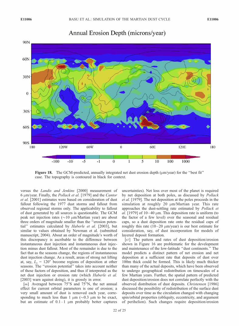
versus the Landis and Jenkins [2000] measurement of6 mm/year. Finally, the Pollack et al. [1979] and the Cantoret al. [2001] estimates were based on consideration of dustfallout following the 1977 dust storms and fallout fromobserved regional storms only. The applicability to falloutof dust generated by all sources is questionable. The GCMpeak net injection rates (�10 mm/Martian year) are aboutthree orders of magnitude smaller than the ‘‘erosion poten-tial’’ estimates calculated by Haberle et al. [2003], butsimilar to values obtained by Newman et al. (submittedmanuscript, 2004). About an order of magnitude’s worth ofthis discrepancy is ascribable to the difference betweeninstantaneous dust injection and instantaneous dust injec-tion minus dust fallout. Most of the remainder is due to thefact that as the seasons change, the regions of instantaneousdust injection change. As a result, areas of strong net liftingat, say, Ls = 120� become regions of deposition at otherseasons. The ‘‘erosion potential’’ takes into account neitherof these factors of deposition, and thus if interpreted as thenet dust injection or erosion rate (which Haberle et al.[2003] warn against doing), it is grossly in error.[66] Averaged between 75�S and 75�N, the net annual

effect for current orbital parameters is one of erosion; avery small amount of dust is removed each year, corre-sponding to much less than 1 mm (�0.3 mm to be exact,but an estimate of 0.1–1 mm probably better captures

uncertainties). Net loss over most of the planet is requiredby net deposition at both poles, as discussed by Pollacket al. [1979]. The net deposition at the poles proceeds in thesimulation at roughly 20 mm/Martian year. This rateapproaches the dust-settling rate estimated by Pollack etal. [1979] of 10–40 mm. This deposition rate is uniform (tothe factor of a few level) over the seasonal and residualcaps, so a dust deposition rate onto the residual caps ofroughly this rate (10–20 mm/year) is our best estimate forconsideration, say, of dust incorporation for models oflayered deposit formation.[67] The pattern and rates of dust deposition/erosion

shown in Figure 16 are problematic for the developmentand maintenance of the low-latitude ‘‘dust continents.’’ Themodel predicts a distinct pattern of net erosion and netdeposition at a sufficient rate that deposits of dust over100m thick could be formed. This is likely much thickerthan many of the actual deposits, which have been observedto undergo geographical redistribution on timescales of afew Martian years. Further, the spatial pattern of predicteddust deposition/erosion does not correlate perfectly with theobserved distribution of dust deposits. Christensen [1986]discussed the possibility of redistribution of the surface dustdeposits over time as the circulation changed with changingspin/orbital properties (obliquity, eccentricity, and argumentof perihelion). Such changes require deposition/erosion

Figure 18. The GCM-predicted, annually integrated net dust erosion depth (mm/year) for the ‘‘best fit’’case. The topography is contoured in black for context.


22 of 25

E11006

rates of �10 mm/year, which are not far from the highervalues found over a good fraction (maybe a quarter) of theplanet between 50�S and 50�N.

7. Summary and Conclusions

[68] This paper presents results from GCM simulations ofan interactive dust cycle on Mars. The version of the GFDLMars GCM used in this study differs from that described byFenton and Richardson [2001], Richardson and Wilson[2002], Richardson et al. [2002], and Mischna et al.[2003]. Instead of a dust injection scheme based only onthe surface-air temperature contrast, the present modelincludes detailed, physically based parameterizations ofdust lifting, similar to the approach of Newman et al.[2002a]. These schemes represent the injection of dust byconvective motions, using thermodynamic theory of dustdevils [Renno et al., 1998, 2000], applied on the coarseresolution of the GCM grid, and by large-scale windstresses, using a functional dependence on the frictionalvelocity [Shao, 2001]. As before, the model treats dust as atransportable trace species, the dust distribution beingaffected by the model-resolved winds, subgrid-scale diffu-sion, and particle-mass-dependent sedimentation. The dustis radiatively active in the GCM, influencing thermalinfrared and visible radiative heating of the atmosphere.[69] The convective and resolved-wind dust injection

schemes introduce three free parameters. A given simula-tion, extending for multiple Martian years, uses spatiallyand temporally fixed values for each of these free param-eters. These parameters are the rate constants applied to thetwo injection schemes (simple multipliers) and the thresholdlifting stress for the resolved-wind lifting scheme. Convec-tive lifting is prescribed without a threshold. We chose touse the seasonal cycle of globally averaged air temperaturesas our primary quantitative means of assessing the quality ofthe GCM simulations. The first question we address withthe model is whether the injection schemes can generate adust cycle in agreement with observations, and what com-bination(s) of parameters allow the best fit. We find that theshape of the seasonal air temperature curve in northernspring and summer, when air temperatures are observed tobe highly repeatable [Liu et al., 2003], can be fit either bythe convective lifting scheme or by the stress-lifting schemewith low values of stress-threshold and lifting rate. Thenorthern spring and summer temperatures cannot be fit ifthe dust opacity only results from the fallout of dust from aglobal storm in the previous southern summer. Both theconvective and low-threshold stress-lifting schemes requiresteady and widespread dust lifting throughout northernspring and summer. Widespread convective (dust devil)lifting seems consistent with the widespread observationof dust devils and dust devil tracks, and indeed the modelpredicts injection rates that are in good agreement withanalysis of Imager for Mars Pathfinder data [Ferri et al.,2003]. Widespread wind stress lifting seems much lessconsistent with the relatively few and sporadic local duststorms observed in northern summer [Cantor et al., 2001].Specifically, cap edge storms, other local dust storms, andlifting associated with dust streak formation appear insuffi-ciently frequent. Further work is needed to provide quanti-tative support for these qualitative arguments. However, on

the basis of the model results and inferences from observa-tions, we propose that dust devils are the primary dynamicalsystem providing the dust injection necessary to sustain thebackground haze on Mars.[70] Regardless of the convective scheme rate parameter,

dust storms cannot be generated in the model. From this wesuggest that dust devils are not the precursors of duststorms, in agreement with imaging observations. It is alsonot possible to generate dust storms with the stress-liftingscheme set with parameter values necessary to sustain thebackground dust haze. Conversely, with stress values andinjection rates high enough to initiate storm activity, liftingdoes not occur throughout much of northern spring andsummer. Simulation of the dust cycle involving storms andthe background haze requires two schemes: a combinationof high-rate, high-threshold lifting, and either convectivelifting or low-threshold, low-rate stress lifting. Justificationfor the use of two different sets of injection parameters intwo parallel stress-lifting schemes is possible, but seems amore complex and observationally less-well supportedsolution than the convective plus high-threshold injectionscheme option. When run with a combination of convectiveand high-threshold dust injection schemes, the model is ableto generate both a realistic background dust cycle, and forthe first time, spontaneous and interannually (and intra-annually) variable global dust storms. These storms arediscussed in greater detail by B04.[71] Varying injection parameters, a multiyear ‘‘best fit’’

simulation can been produced with optimal air temperatureand dust storm emulation. This simulation uses convectiveand high-threshold stress lifting. The model develops arange of local and regional storms, the variety and distri-bution of which compares reasonably well with observa-tions [Cantor et al., 2001]. Specifically, seasonal ice-capedge dust storms are simulated, as are storms associatedwith various topographic features. Comparison with airtemperature cross section data suggest that cap edge liftingis somewhat underpredicted. Several small dust storms aregenerated in the northern early autumn and later winter,associated with low-pressure frontal storms, as described byWang et al. [2003], and also generated in the Oxford MarsGCM [Newman et al., 2002b]. One such storm developsinto a large regional event, resembling the 1999 storm andthe dust storm that preceded the Mars Exploration Roverlandings (B04). The model also predicts the distribution andseasonal variation of dust devil activity (if the convectivelifting is ascribed to dust devils). A distinct peak in activityis found in the model in Amazonis, a region of observedenhanced dust devil activity.[72] The rates of dust injection and the net removal/

deposition of dust on the surface are predictions of themodel. It has not been possible to predict annuallyintegrated net dust deposition/erosion rates until this pointas it requires a validated dust cycle that includes interactivelifting, transport, and deposition of dust. Previous estimatesof dust erosion have had to rely on ‘‘lifting potential’’derived from the model wind stresses to predict liftingand have ignored the other side of the cycle: deposition[Haberle et al., 2003]. Our results suggest that net, annuallyintegrated erosion/deposition rates are roughly one to twoorders of magnitude lower when the full dust cycle is takeninto account. Thus extreme caution must be taken when


23 of 25

E11006

interpreting the previously generated ‘‘lifting potential’’erosion values. Net annual erosion/deposition rates com-pare well with estimates from the Mars Pathfinder solarpanel experiment [Landis and Jenkins, 2000] and fromanalysis of the darkening of slope streaks [Aharonson etal., 2003]. Between 75�S and 75�N, the net annualerosion rate is 0.3 mm/Martian year (0.1–1 mm/Martianyear, conservatively), which is balanced by net polardeposition at roughly 20 mm/Martian year, consistent withestimates from Pollack et al. [1979]. Although thesevalues are the best possible GCM estimate at this time,the model still neglects processes of potential importance,including dust-ice interactions. These must be assessed infuture models.

[73] Acknowledgments. S.B. and M.I.R. were supported by NSFPlanetary Astronomy Award number 0406653. R.J.W. was supported bythe NASA Planetary Atmospheres program grant. We thank our referees,Richard Zurek and anonymous reviewer, for useful suggestions. We alsothank Claire E. Newman and A. P. Ingersoll for useful discussions.

ReferencesAharonson, O., N. Schorghofer, and M. F. Gerstell (2003), Slope streakformation and dust deposition rates on Mars, J. Geophys. Res., 108(E12),5138, doi:10.1029/2003JE002123.

Balme, M. R., P. L. Whelley, and R. Greeley (2003), Mars: Dust devil tracksurvey in Argyre Planitia and Hellas Basin, J. Geophys. Res., 108(E8),5086, doi:10.1029/2003JE002096.

Banfield, D., et al. (2003), Forced waves in the Martian atmosphere fromMGS TES nadir data, Icarus, 161, 319–345.

Briggs, G. A., W. A. Baum, and J. Barnes (1979), Viking Orbiter imagingobservations of dust in the Martian atmosphere, J. Geophys. Res., 84,2795–2820.

Cantor, B. A., and K. S. Edgett (2002), Martian dust devils: 2 Mars years ofMGS MOC observations, Eos Trans. AGU, 83(47), Fall Meeting Suppl.,Abstract P51A-0331.

Cantor, B. A., P. B. James, M. Caplinger, and M. J. Wolff (2001), Martiandust storms: 1999 Mars Orbiter Camera observations, J. Geophys. Res.,106, 23,653–23,687.

Cantor, B., M. Malin, and K. S. Edgett (2002), Multiyear Mars OrbiterCamera (MOC) observations of repeated Martian weather phenomenaduring the northern summer season, J. Geophys. Res., 107(E3), 5014,doi:10.1029/2001JE001588.

Christensen, P. R. (1986), Regional dust deposits on Mars: Physical proper-ties, age and history, J. Geophys. Res., 91, 3533–3545.

Clancy, R. T., D. O. Muhleman, and G. L. Berge (1990), Global changes inthe 0–70 km thermal structure of the Mars atmosphere derived from1975 to 1989 microwave CO spectra, J. Geophys. Res., 95, 14,543–14,554.

Clancy, R. T., A. W. Grossman, M. J. Wolff, P. B. James, D. J. Rudy, Y. N.Billawala, B. J. Sandor, S. W. Lee, and D. O. Muhleman (1996), Watervapor saturation at low altitudes around Mars aphelion: A key to Marsclimate?, Icarus, 122, 36–62.

Clancy, R. T., B. J. Sandor, M. J. Wolff, P. R. Christensen, M. D. Smith,J. C. Pearl, B. J. Conrath, and R. J. Wilson (2000), An intercomparison ofground-based millimeter, MGS TES, and Viking atmospheric temperaturemeasurements: Seasonal and interannual variability of temperatures anddust loading in the global Mars atmosphere, J. Geophys. Res., 105(E4),9553–9572.

Colburn, D. S., J. B. Pollack, and R. M. Haberle (1989), Diurnal variationsin optical depth at Mars, Icarus, 79, 159–189.

Conrath, B. J., J. C. Pearl, M. D. Smith, W. C. Maguire, P. R. Christensen,S. Dason, and M. S. Kaelberer (2000), Mars Global Surveyor ThermalEmission Spectrometer (TES) observations: Atmospheric temperaturesduring aerobraking and science phasing, J. Geophys. Res., 105, 9509–9519.

Fenton, L. K., and M. I. Richardson (2001), Martian surface winds: Insen-sitivity to orbital changes and implications for aeolian processes, J. Geo-phys. Res., 106, 32,885–32,902.

Fenton, L. K., J. C. Pearl, and T. Z. Martin (1997), Mapping Mariner 9 dustopacities, Icarus, 130, 115–124.

Ferri, F., P. H. Smith, M. Lemmon, and N. O. Renno (2003), Dust devils asobserved by Mars Pathfinder, J. Geophys. Res., 108(E12), 5133,doi:10.1029/2000JE001421.

Fisher, J., et al. (2002), A survey of Martian dust devil activity using MarsGlobal Surveyor Mars Orbiter camera images, Eos Trans. AGU, 83(47),Fall Meet. Suppl., Abstract P01-5742.

Forget, F., F. Hourdin, R. Fournier, C. Hourdin, O. Talagrand, M. Collins,S. R. Lewis, P. L. Read, and J. P. Huot (1999), Improved general circula-tion model of the Martian atmosphere from the surface to above 80 km,J. Geophys. Res., 104, 24,155–24,175.

Gierasch, P. J., and R. M. Goody (1968), A study of the thermal anddynamical structure of the Martian lower atmosphere, Planet. SpaceSci., 16, 615–646.

Greeley, R., N. Lancaster, S. Lee, and P. Thomas (1992), Martian Aeolianprocesses, sediments and features, in Mars, edited by H. H. Kieffer et al.,pp. 730–776, Univ. of Ariz. Press, Tucson.

Haberle, R. M., J. B. Pollack, J. R. Barnes, R. W. Zurek, C. B. Leovy, J. R.Murphy, H. Lee, and J. Schaeffer (1993), Mars atmospheric dynamiccirculation as simulated by the NASA Ames general circulation model:The zonal mean circulation, J. Geophys. Res., 98, 3093–3123.

Haberle, R. M., J. R. Murphy, and J. Schaeffer (2003), Orbital changeexperiments with a Mars general circulation model, Icarus, 161, 66–89.

Hamilton, K. (1995), Interannual variability in the northern hemispherewinter middle atmosphere in control and perturbed experiments withthe GFDL SKYHI general circulation model, J. Atmos. Sci., 52, 44–66.

Hanel, R. C., et al. (1972), Investigation of Martian environment by infraredspectroscopy on Mariner 9, Icarus, 17, 423–442.

Hinson, D. P., and R. J. Wilson (2002), Transient eddies in the southernhemisphere of Mars, Geophys. Res. Lett., 29(7), 1154, doi:10.1029/2001GL014103.

Hinson, D. P., and R. J. Wilson (2004), Temperature inversions, thermaltides, and water ice clouds in the Martian tropics, J. Geophys. Res., 109,E01002, doi:10.1029/2003JE002129.

Hollingsworth, J. L., R. M. Haberle, J. R. Barnes, A. F. C. Brider, J. B.Pollack, H. Lee, and J. Schaeffer (1996), Orographic control of stormzones on Mars, Nature, 380, 413–416.

Kahn, R. A., T. Z. Martin, R. W. Zurek, and S. W. Lee (1992), The Martiandust cycle, in Mars, edited by H. H. Kieffer et al., pp. 1017–1053, Univ.of Ariz. Press, Tucson.

Kieffer, H. H., and A. P. Zent (1992), Quasi-periodic climate change onMars, in Mars, edited by H. H. Kieffer et al., pp. 1180–1220, Univ. ofAriz. Press, Tucson.

Landis, G. A., and P. P. Jenkins (2000), Measurement of the settling rate ofatmospheric dust on Mars by the MAE instrument on Mars Pathfinder,J. Geophys. Res., 105, 1855–1857.

Leovy, C. B., G. Briggs, A. Young, B. Smith, J. Pollack, E. Shipley,and R. Widley (1972), The Martian atmosphere: Mariner 9 televisionexperiment progress report, Icarus, 17, 373–393.

Liu, J., M. I. Richardson, and R. J. Wilson (2003), An assessment of theglobal, seasonal, and interannual spacecraft record of Martian climate inthe thermal infrared, J. Geophys. Res., 108(E8), 5089, doi:10.1029/2002JE001921.

Lorenz, R. D., J. I. Lunine, J. A. Grier, and M. A. Fisher (1996), Martiansurface wind speeds described by the Weibull distribution, J. Spacecr.Rockets, 33, 754–756.

Magalhaes, J. A., and R. E. Young (1995), Downslope windstorms in thelee of ridges on Mars, Icarus, 113, 277–294.

Malin, M., and K. S. Edgett (2001), Mars Global Surveyor Mars OrbiterCamera: Interplanetary cruise through primary mission, J. Geophys. Res.,106, 23,429–23,570.

Martin, L. J., and R. W. Zurek (1993), An analysis of the history of dustactivity on Mars, J. Geophys. Res., 98, 3221–3246.

Martin, T. Z. (1981), Mean thermal and albedo behavior of the Mars surfaceand atmosphere over a Martian year, Icarus, 45, 427–446.

Martin, T. Z. (1986), Thermal Infrared opacity of the Mars atmosphere,Icarus, 66, 2–21.

Martin, T. Z., and H. H. Kieffer (1979), Thermal infrared properties of theMartian atmosphere: 2. The 15-mm band measurements, J. Geophys. Res.,84, 2843–2852.

Martin, T. Z., and M. I. Richardson (1993), New dust opacity mapping fromViking infrared thermal mapper data, J. Geophys. Res., 98, 10,941–10,949.

Metzger, S. M., J. R. Carr, J. R. Johnson, T. J. Parker, and M. T. Lemmon(1999), Dust devil vortices seen by Mars Pathfinder Camera, Geophys.Res. Lett., 26, 2781–2784.

Mischna, M. A., M. I. Richardson, R. J. Wilson, and D. J. McCleese (2003),On the orbital forcing of Martian water and CO2 cycles: A generalcirculation model study with simplified volatile schemes, J. Geophys.Res., 108(E6), 5062, doi:10.1029/2003JE002051.

Moore, H. J. (1985), The Martian dust storm of Sol-1742, Proc. LunarPlanet. Sci. Conf. 16th, Part 1, J. Geophys. Res., 90, suppl., D163–D174.


24 of 25

E11006

Murphy, J. R., and S. Nelli (2002), Mars Pathfinder convective vortices:Frequency of occurrence, Geophys. Res. Lett., 29(23), 2103, doi:10.1029/2002GL015214.

Murphy, J. R., O. B. Toon, R. M. Haberle, and J. B. Pollack (1990),Numerical simulations of the decay of Martian global dust storms,J. Geophys. Res., 95, 14,629–14,648.

Newman, C. E., S. R. Lewis, P. L. Read, and F. Forget (2002a), Modelingthe Martian dust cycle, 1. Representations of dust transport processes,J. Geophys. Res., 107(E12), 5123, doi:10.1029/2002JE001910.

Newman, C. E., S. R. Lewis, P. L. Read, and F. Forget (2002b), Modelingthe Martian dust cycle 2. Multiannual radiatively active dust transportsimulations, J. Geophys. Res., 107(E12), 5124, doi:10.1029/2002JE001920.

Pollack, J. B., D. Colburn, F. M. Flasar, R. Kahn, C. E. Carlston, andD. Pidek (1979), Properties and effects of dust particles suspended inthe Martian atmosphere, J. Geophys. Res., 84, 2929–2945.

Read, P. L., M. Collins, F. Forget, R. Fournier, F. Hourdin, S. R. Lewis,O. Talagrand, F. W. Taylor, and N. P. J. Thomas (1997), A GCM climatedatabase for Mars: For mission planning and scientific studies, Adv.Space Res., 19, 1213–1222.

Renno, N. O., M. L. Burket, and M. P. Larkin (1998), A simple thermo-dynamic theory for dust devils, J. Atmos. Sci., 55, 3244–3252.

Renno, N. O., A. A. Nash, J. Lunine, and J. Murphy (2000), Martian andterrestrial dust devils: Test of a scaling theory using Pathfinder data,J. Geophys. Res., 105, 1859–1865.

Richardson, M. I. (1998), Comparison of microwave and infrared measure-ments of Martian atmosphere temperatures: Implications for short termclimate variability, J. Geophys. Res., 103, 5911–5918.

Richardson, M. I., and R. J. Wilson (2002), Investigation of the nature andstability of the Martian seasonal water cycle with a general circulationmodel, J. Geophys. Res., 107(E5), 5031, doi:10.1029/2001JE001536.

Richardson, M. I., R. J. Wilson, and A. V. Rodin (2002), Water ice cloudsin the Martian atmosphere: General circulation model experiments witha simple cloud scheme, J. Geophys. Res., 107(E9), 5064, doi:10.1029/2001JE001804.

Seguro, J. V., and T. W. Lambert (2000), Modern estimation of theparameters of the Weibull wind speed distribution for wind energyanalysis, J. Wind Eng. Ind. Aerodyn., 85, 75–84.

Shao, Y. (2001), Physics and Modeling of Wind Erosion, pp. 113–316,Kluwer Acad., Norwell, Mass.

Smith, M. D. (2004), Inerannual variability in TES atmospheric observa-tions of Mars during 1999–2003, Icarus, 167, 148–165.

Smith, M. D., J. C. Pearl, B. J. Conrath, and P. R. Christensen (2001),Thermal Emission Spectrometer results: Mars atmospheric thermalstructure and aerosol distribution, J. Geophys. Res., 106, 23,929–23,945.

Smith, M. D., R. J. Conrath, J. C. Pearl, and P. R. Christensen (2002),Thermal Emission Spectrometer observations of Martian planetencircling dust storm 2001A, Icarus, 157, 259–263.

Smith, P. H., and M. Lemmon (1999), Opacity of the Martian atmospheremeasured by the images from Mars Pathfinder, J. Geophys. Res., 104,8975–8985.

Thomas, P., and P. J. Gierasch (1985), Dust devils on Mars, Science, 230,175–177.

Thomas, P., J. Veverka, S. Lee, and A. Bloom (1981), Classification ofwind streaks on Mars, Icarus, 45, 124–153.

Thomas, P., J. Veverka, D. Gineris, and L. Wong (1984), Dust streaks onMars, Icarus, 60, 161–179.

Thomas, P. C., P. Gierasch, R. Sullivan, D. S. Miller, E. A. del Castillo,B. Cantor, and M. T. Mellon (2003), Meso-scale linear streaks on Mars:Environments of dust entrainment, Icarus, 162, 242–258.

Toigo, A. D., and M. I. Richardson (2000), Seasonal variation of aerosols inthe Martian atmosphere, J. Geophys. Res., 105, 4109–4121.

Toigo, A. D., M. I. Richardson, S. P. Ewald, and P. J. Gierasch (2003),Numerical simulation of Martian dust devils, J. Geophys. Res., 108(E6),5047, doi:10.1029/2002JE002002.

Wang, H., M. I. Richardson, R. J. Wilson, A. P. Ingersoll, A. D. Toigo, andR. W. Zurek (2003), Cyclones, tides, and the origin of a cross-equatorialdust storm on Mars, Geophys. Res. Lett., 30(9), 1488, doi:10.1029/2002GL016828.

White, B. R. (1979), Soil transport by winds on Mars, J. Geophys. Res., 84,4643–4651.

Wilson, R. J. (1997), A general circulation model simulation of the Martianpolar warming, Geophys. Res. Lett., 24, 123–127.

Wilson, R. J. (2000), Evidence for diurnal period Kelvin waves in theMartian atmosphere from Mars Global Surveyor TES data, Geophys.Res. Lett., 27, 3889–3892.

Wilson, R. J., and K. Hamilton (1996), Comprehensive model simulationsof thermal tides in the Martian atmosphere, J. Atmos. Sci., 53, 1290–1326.

Wilson, R. J., and M. I. Richardson (1999), Comparison of Mars GCM duststorm simulations with Viking mission observations, in Fifth Interna-tional Conference on Mars [CD-ROM], LPI Contrib. 972, abstract6234, Lunar and Planet. Inst., Houston, Tex.

Wilson, R. J., and M. I. Richardson (2000), The Martian atmosphere duringthe Viking mission, 1, Infrared measurements of atmospheric tempera-tures revisited, Icarus, 145, 555–579.

Wilson, R. J., D. Banfield, B. J. Conrath, and M. D. Smith (2002), Travel-ing waves in the northern hemisphere of Mars, Geophys. Res. Lett.,29(14), 1684, doi:10.1029/2002GL014866.

Zurek, R. W., J. R. Barnes, R. M. Haberle, J. B. Pollack, J. E. Tillman, andC. B. Leovy (1992), Dynamics of the atmosphere of Mars, in Mars,edited by H. H. Kieffer, pp. 835–933, Univ. of Ariz. Press, Tucson.

��S. Basu and M. I. Richardson, Division of Geological and Planetary

Sciences, California Institute of Technology, MC 150-21 Caltech, 1200 EastCalifornia Boulevard, Pasadena, CA 91125, USA. ([email protected])R. J. Wilson, Geophysical Fluid Dynamics Laboratory, National Oceanic

and Atmospheric Administration, P.O. Box 308, Princeton, NJ 08542,USA.


25 of 25

E11006

Documents

Simulation of the Martian dust cycle with the GFDL Mars GCMSimulation of the Martian dust cycle with the GFDL Mars GCM Shabari Basu and Mark I. Richardson Division of Geological and