SIMULATION OF THE FEED-IN POWER OF DISTRIBUTED PV SYSTEMS

LISA GROSSI(1) • GEORG WIRTH(1) • ELKE LORENZ(2) • ANDREAS SPRING(1) • GERD BECKER(1)

(1) University of Applied Sciences Munich · Department of Electrical Engineering · 80335 Munich · Germany ·

Phone +49 (0) 89 1265-4412 · lgrossi@hm.edu

(2) Carl von Ossietzky Universität Oldenburg · Fakultät V · Institut für Physik · AG Energiemeteorologie · Germany

ABSTRACT: In Southern Germany a high number of photovoltaic (PV) plants feeds into the grid. New load patterns

occur and with them changed grid requirements. Feed-in management is one possibility to maintain grid stability and

safety. Nowadays feed-in management measures are carried out in defined steps (typically: 100%, 60%, 30%, 0% of

PSTC). As the power produced by PV plants depends on the current irradiance situation, the reduction of the feed-in

power according to a predefined level mostly does not lead to the desired effect in the grid. Thus, the network operator

needs detailed knowledge of the condition of the grid in order to be able to carry out targeted regulating measures.

This paper presents a simulation model that allows to model the feed-in power of a distributed PV fleet and to

characterize the consumption in the medium and low voltage grid of the investigated area. On the one hand, the

simulation is carried out on the basis of irradiance data recorded by a spatially distributed high resolution measurement

system. On the other hand, satellite data is used as simulation input. Simulation accuracy of both variants is compared

and their advantages and disadvantages discussed.

Keywords: Grid-Connected, Grid Integration, Grid Management, Grid Stability, Simulation

1 INTRODUCTION

The increasing share of renewable energies in the

German power supply leads to changed grid requirements

that must be met by the network operator to maintain grid

stability and safety [6]. In this context Bayernwerk AG

has initiated the project “Netz der Zukunft” (“Grid of the

Future”) in cooperation with the University of Applied

Sciences München and Technische Universität München.

A medium voltage grid is analysed in order to examine

the impact of photovoltaic (PV) systems on the grid. The

investigated grid is situated in a rural area in Northern

Bavaria and characterized by a very high PV penetration.

Altogether 36 MW of PV capacity are installed. This

amounts to ca. 5.6 kW per house connection. Smart

meters record data at every substation (110-20 kV and

20-0.4 kV) and at many house connections with and

without PV power plants. Thus, highly resolved grid

measurements are available.

In order to determine the behaviour of a distributed PV

fleet, the spatial distribution of the irradiation in the

investigated area is analysed. A special focus thereby is

to characterize the geographic smoothing of the feed-in

power on days with fluctuating cloud covers.

Therefore, a high resolution measurement system records

global irradiation and temperature. The distributed fleet

and the ten measurement stations are spread over an area

of ca. 11x15 km. The acquired data is being used to

simulate the power generation of the distributed PV fleet

in the project area.

A second approach is to use satellite data as simulation

input. The satellite data features a different time and

spatial resolution than the distributed measurement

system.

In the following, the simulation approach in general is

described. Then, the two input data variants are compared

and simulation results are presented.

2 SIMULATION APPROACH

The project area is divided into subareas of which each is

simulated separately. The simulation model is efficiency-

based and uses a PT1 element to model the geographic

smoothing of the feed-in power on days with fluctuating

cloud covers. Its time constant depends on the installed

PV capacity of the corresponding subarea. The approach

is similar to the one presented in [2]. Figure 1 illustrates

the schematic of the simulation process.

Figure 1: Schematic of the simulation process. Each

subarea is simulated separately.

The following variables are used as input: The spatially

distributed measurement devices record global horizontal

irradiance and ambient temperature. First, horizontal

irradiance is converted into global tilted irradiance using

the model presented in Perez et al. [3]. Then, by means of

the recorded ambient temperature, tilted irradiance and

the module-specific parameter γ, the module temperature

is calculated:

The parameter γ depends on the mounting type of the PV

plant [1].

In the next step module efficiency η is determined:

with the parameters α1,α2,α3 describing the part load

behaviour of the modules for a module temperature of

25° C. The parameters depend on the cell type. The

parameter αp corresponds to the temperature coefficient

and describes the module behaviour at module

temperature Tmod. For the simulation model, weighted

average values of α1,α2,α3 and αp representing the

different cell types on the market are used.

Module efficiency η and the installed PV capacity AG

determine the proportional gain Kp. The time constants

have been empirically determined and optimized in

dependency of the size of the subareas. [5] The used

highly resolved data has been recorded in Jülich in

Germany within the framework of the project

HD(CP)²/HOPE. Proportional gain Kp and the time

constant tpt1 are the input parameters of the PT1 element.

Its output is the DC power of the single subareas and

finally the power of the whole distributed PV fleet.

( ( - )) ( - ) (3)

∑ (4)

DC power is converted into AC power using the model

presented by Schmidt and Sauer [4]. Additionally, system

losses of 9.5% are considered [1]

On the basis of the simulated feed-in power and the

cumulated power of the area measured over the 110 kV

substation, that we have at our disposal, a reference load

can be calculated. The load curve is calculated for a clear

sky day and serves as reference for the simulation of

further days. The application of the calculated reference

load requires that the simulation model provides correct

results on a clear day. This assumption has to be made as

no detailed measurement of the load exists. Further,

standard load profiles cannot be applied as too many

special contract customers are situated in the grid area

and strongly influence the area’s load behaviour.

Therefore, simulation accuracy has been validated using

measured PV data. [5] Figure 2 illustrates the simulated

feed-in power, the measured load curve and the resultant

calculated reference load.

Figure 2: Simulated feed-in power (green), cumulated

power of the area measured over the 110 kV

substation (red) and calculated reference load (blue)

on 18 June 2012.

3 THE DISTRIBUTED MEASUREMENT SYSTEM

Ten spatially distributed measurement devices record

global irradiation and temperature. It is a ground based

simulation. Figure 3 illustrates the distributed

measurement in the area.

Figure 3: Ground based measurement points in the

investigated area and the ten subareas. Each subarea

is simulated separately by means of the corresponding

device’s data and installed PV capacity.

Time resolution of the measurement devices amounts to

3 seconds and spatial resolution is ca. 10 km². The single

subareas are simulated using their device’s data and

installed PV capacity and a time constant depending on

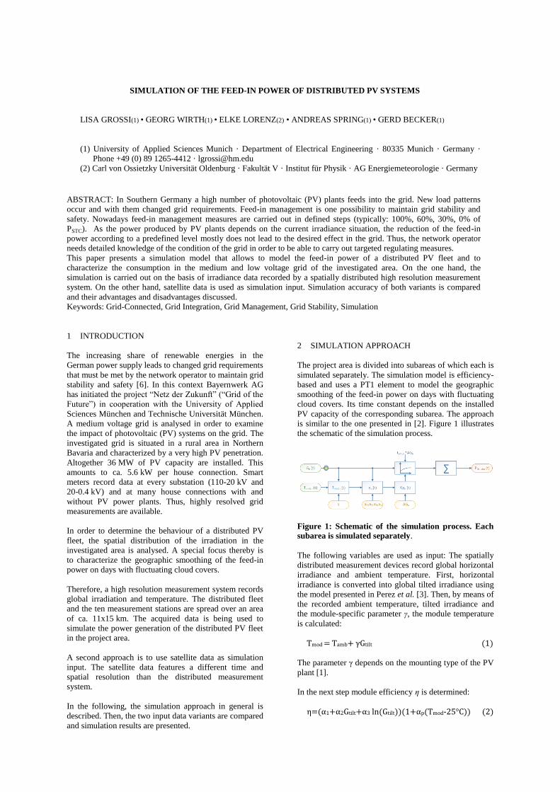
the size of the subarea. Figure 4 illustrates a day with

fluctuating cloud cover simulated on the basis of the

distributed measurement. Measurement and simulation

match rather well. In comparison, figure 5 shows the

same day simulated using just one irradiance value. The

simulated curve differs strongly from the measured one.

One measurement device is not sufficient to model the

smoothing effect of the feed-in power of the distributed

PV systems on days with fluctuating cloud covers. The

grid condition is not described properly.

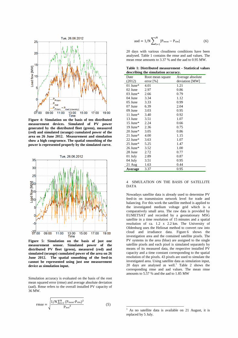
Figure 4: Simulation on the basis of ten distributed

measurement devices. Simulated of PV power

generated by the distributed fleet (green), measured

(red) and simulated (orange) cumulated power of the

area on 26 June 2012. Measurement and simulation

show a high congruence. The spatial smoothing of the

power is represented properly by the simulated curve.

Figure 5: Simulation on the basis of just one

measurement sensor. Simulated power of the

distributed PV fleet (green), measured (red) and

simulated (orange) cumulated power of the area on 26

June 2012. The spatial smoothing of the feed-in

cannot be represented using just one measurement

device as simulation input.

Simulation accuracy is evaluated on the basis of the root

mean squared error (rmse) and average absolute deviation

(aad). Rmse refers to the overall installed PV capacity of

36 MW.

√ ∑

∑

20 days with various cloudiness conditions have been

analysed. Table 1 contains the rmse and aad values. The

mean rmse amounts to 3.37 % and the aad to 0.95 MW.

Table 1: Distributed measurement - Statistical values

describing the simulation accuracy.

Date

(2012)

Root mean square

error [%]

Average absolute

deviation [MW]

01 June* 4.01 1.21

02 June 2.97 0.86

03 June* 2.66 0.79

04 June 3.34 1.12

05 June 3.33 0.99

07 June 6.39 2.04

09 June 3.03 0.95

11 June* 3.40 0.92

13 June 3.51 1.07

15 June* 2.24 0.66

19 June* 2.36 0.75

20 June* 3.05 0.86

21 June* 4.00 1.15

22 June* 3.63 1.07

25 June* 5.25 1.47

26 June* 3.52 1.00

28 June 2.72 0.77

01 July 2.89 0.87

04 July 3.51 0.95

21 Aug 1.63 0.44

Average 3.37 0.95

4 SIMULATION ON THE BASIS OF SATELLITE

DATA

Nowadays satellite data is already used to determine PV

feed-in on transmission network level for trade and

balancing. For this work the satellite method is applied to

the investigated medium voltage grid which is a

comparatively small area. The raw data is provided by

EUMETSAT and recorded by a geostationary MSG

satellite in a time resolution of 15 minutes and a spatial

resolution of ca. 1.2 x 2.2 km. The University of

Oldenburg uses the Heliosat method to convert raw into

cloud and irradiance data. Figure 6 shows the

investigation area and the contained satellite pixels. The

PV systems in the area (blue) are assigned to the single

satellite pixels and each pixel is simulated separately by

means of its measured data, the respective installed PV

capacity and a time constant corresponding to the spatial

resolution of the pixels. 43 pixels are used to simulate the

investigated area. Using satellite data as simulation input,

20 days are analysed as well.1 Table 2 shows the

corresponding rmse and aad values. The mean rmse amounts to 5.57 % and the aad to 1.85 MW

1 As no satellite data is available on 21 August, it is

replaced by 5 July.

Figure 6: Investigation area and measurement points

(red) covered by satellite. The blue markers indicate

PV systems.

Table 2: Satellite data - Statistical values describing

the simulation accuracy.

Date

(2012)

Root mean square

error [%]

Average absolute

deviation [MW]

01 June 6.77 2.09

02 June 5.35 1.61

03 June 5.03 2.76

04 June 4.86 1.57

05 June 3.92 1.19

07 June 5.71 1.83

09 June 8.43 2.87

11 June 4.94 1.23

13 June 5.88 1.88

15 June 4.09 1.49

19 June 6.67 2.17

20 June 4.02 1.83

21 June 5.79 1.71

22 June 6.49 2.21

25 June 4.34 1.77

26 June 5.81 1.85

28 June 6.74 2.10

01 July 8.33 2.26

04 July 3.66 1.19

05 July 4.56 1.35

Average 5.57 1.85

5 COMPARISON OF THE TWO APPROACHES

The evaluation of the 20 exemplary days shows that the

simulation on the basis of the distributed ground based

measurement features a higher accuracy than the one

based on satellite data. This is mainly due to the fact that

cloud shadows cannot be precisely assigned to one single

pixel. To determine the cloud shadows, an average height

of the clouds is assumed leading to inaccuracies in a

small scale simulation. The advantage of satellite data is

that no measurement system has to be built up and

maintained. The data is available anyway. Figure 7

illustrates a cloudy day simulated with the data of the

distributed measurement. Figure 8 shows the same day

based on the satellite data. Measurement and simulation

show a good match. Simulated load flow is located

slightly below the measured curve.

Figure 7: Simulation on the basis of the ten ground

based distributed measurement devices in 15 minute

resolution. Simulated power of the distributed PV

fleet (green), measured (red) and calculated (orange)

cumulated power of the area on 26 June 2012. Data

from the distributed measurement is used as input.

Figure 8: Simulation on the basis of satellite data.

Simulated power of generated by the distributed PV

fleet (green), measured (red) and calculated (orange)

cumulated power of the area on 26 June 2012 based

on the satellite data.

Figure 9 shows the simulation accuracy of the distributed

system in 3 second resolution depending on the number

of measurement devices used as simulation input. Only

days marked with an asterisk (*) in Table 1 are evaluated.

The simulation with ten devices features a high accuracy

of about 3.5 % in average. Using only one measurement

sensor leads to low accuracy values as already seen in

figure 5. Average rmse amounts to ca. 11.5 %. The

satellite based simulation features an average rmse of

5.6 %, which is approximately as high as the distributed

simulation in 3 second resolution with 6 measurement

devices.

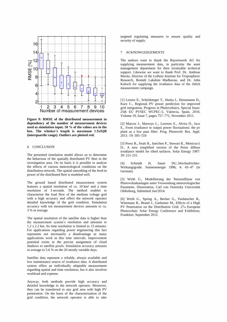
Figure 9: RMSE of the distributed measurement in

dependency of the number of measurement devices

used as simulation input. 50 % of the values are in the

box. The whisker’s length is maximum 1.5xIQR

(interquartile range). Outliers are plotted red.

6 CONCLUSION

The presented simulation model allows us to determine

the behaviour of the spatially distributed PV fleet in the

investigation area. On its basis it is possible to analyse

the effects of various meteorological conditions on the

distribution network. The spatial smoothing of the feed-in

power of the distributed fleet is modeled well.

The ground based distributed measurement system

features a spatial resolution of ca. 10 km² and a time

resolution of 3 seconds. The method enables to

characterize the load flow of the medium voltage grid

with a high accuracy and offers the network operator

detailed knowledge of the grid condition. Simulation

accuracy with ten measurement devices amounts to ca.

3 % in average.

The spatial resolution of the satellite data is higher than

the measurement system’s resolution and amounts to

1.2 x 2.2 km. Its time resolution is limited to 15 minutes.

For applications regarding power engineering this fact

represents not necessarily a disadvantage as many

applications work in this time intervals. Improvement

potential exists in the precise assignment of cloud

shadows to satellite pixels. Simulation accuracy amounts

in average to 5.6 % on the 20 mostly variable days.

Satellite data represent a reliable, always available and

low maintenance source of irradiance data. A distributed

system offers an individually adaptable measurement

regarding spatial and time resolution, but it also involves

workload and expense.

Anyway, both methods provide high accuracy and

detailed knowledge to the network operator. Moreover,

they can be transferred to any grid area with high PV

penetration. On the basis of the characterization of the

grid condition, the network operator is able to take

targeted regulating measures to ensure quality and

security of supply.

7 ACKNOWLEDGEMENTS

The authors want to thank the Bayernwerk AG for

supplying measurement data, in particular the asset

management department for their invaluable technical

support. Likewise we want to thank Prof. Dr. Andreas

Macke, Director of the Leibniz Institute for Tropospheric

Research, Bomidi Lakshmi Madhavan, and Dr. John

Kalisch for supplying the irradiance data of the Jülich

measurement campaign.

[1] Lorenz E., Scheidsteger T., Hurka J., Heinemann D.,

Kurz C., Regional PV power prediction for improved

grid integration, Progress in Photovoltaics, Special Issue:

25th EU PVSEC WCPEC-5, Valencia, Spain, 2010,

Volume 19, Issue 7, pages 757–771, November 2011.

[2] Marcos J., Marroyo L., Lorenzo E., Alvira D., Izco

E., From irradiance to output power fluctuations: the pv

plant as a low pass filter. Prog. Photovolt: Res. Appl.

2011: 19: 505–510

[3] Perez R., Seals R., Ineichen P., Stewart R., Menicucci

D., A new simplified version of the Perez diffuse

irradiance model for tilted surfaces. Solar Energy 1987:

39: 221-231.

[4] Schmidt H, Sauer DU.,Wechselrichter-

Wirkungsgrade. Sonnenenergie 1996; 4: 43–47 (in

German).

[5] Wirth G., Modellierung der Netzeinflüsse von

Photovoltaikanlagen unter Verwendung meteorologischer

Parameter, Dissertation, Carl von Ossietzky Universität

Oldenburg, Submitted Jun/2014.

[6] Wirth G., Spring A., Becker G., Pardatscher R.,

Witzmann R., Brantl J., Garhamer M., Effects of a High

PV Penetration on the Distribution Grid. 27th European

Photovoltaic Solar Energy Conference and Exhibition,

Frankfurt, September 2012.