Simulation of the density of states in isothermal and adiabatic ensembles

Simulation of the density of states in isothermal and adiabatic ensembles

Fernando A. EscobedoSchool of Chemical and Biomolecular Engineering, Cornell University, Ithaca, New York 14853, USA

�Received 4 February 2006; published 8 May 2006�

This paper provides a unified treatment of the fundamental methods used to obtain the density of states � viamolecular simulations with isothermal ensembles �IEs� and adiabatic ensembles �AEs�. Our analysis andresults show that � provides a natural bridge to go back and forth between IE and AE simulation data. Theyalso underline the difference between the density of states of potential energy macrostates � and that of totalenergy macrostates �, even though both provide access to the thermodynamic properties of the system.Visited-states approaches and transition matrix methods are described and applied to the Lennard-Jones fluid totarget � and � as functions of energy and volume macrostates. It is shown that one can obtain � via ageneralized acceptance-ratio formula that is applicable regardless of the conditions at which the ensemble issimulated. In this way, one can obtain � while performing conventional IE or AE simulations, and do it at noextra cost and with a higher accuracy than is achievable with histogram methods.

DOI: 10.1103/PhysRevE.73.056701 PACS number�s�: 02.70.Tt, 05.10.Ln, 02.70.�c

I. INTRODUCTION

Molecular simulations with conventional statistical me-chanical ensembles are still the main route to access the ther-modynamic properties of a system �1,2�. In such simulations,one primarily collects information about ensemble averagesof key quantities of the system which can, directly or indi-rectly, be connected to macroscopic, thermodynamic proper-ties. Such key quantities will be denoted macrostate variablesor macrovariables and are extensive properties that fluctuatein the simulation. In recent years, it has been recognized thatsimulation methods able to extract density of states � data�as a function of the macrovariables� are particularly efficientin mapping out thermodynamic properties over broad rangesof conditions �1–10�. Ensemble averages can be easily ob-tained from � by using straightforward statistical mechanicalformulas. One of the best-known approaches relies on esti-mating � from the histogram�s� that record�s� the variationsof the ensemble macrovariables �3�. In practice, multiple his-tograms, corresponding to simulations at different statepoints, are collected and combined via the multihistogramreweighting �MHR� method �4�; � is extracted �within amultiplicative factor� that is usable over the macrovariabledomain sampled during the simulations. Often, � itself is notobtained or reported but remains implicit in the equationsused for reweighing the thermodynamic properties of inter-est. In some applications, a free-energy function I, ratherthan �, is the property of interest or is the underlying func-tion that allows the reweighting �9–16�. MHR is a “visited-states” method in that � or I comes from data on the fre-quency with which the system visited different macrostates.More recently, another class of methods has been developedwherein one gets � or I not from histogram data but fromdata on the attempted transitions between macrostates�17–25�. Such transition probability or transition matrix�TM� methods have been shown to be more robust and ac-curate than visited-states methods but, as of now, are still farless popular than visited-states methods.

The methods described above have been extensively usedwith isothermal ensembles �IEs�, i.e., those where the tem-perature is fixed in the simulation. The MHR method has

been used with the canonical and grand canonical ensembles�2–8,16�. TM methods have been used, for example, with thecanonical ensemble as the core from which I functions aregenerated and reweighted to get properties associated withgrand canonical, isobaric-isothermal, and semigrand en-sembles �20–25�. Recently �26�, it has been shown that MHRand a particular type of TM method can also be used withany adiabatic ensemble �AE�, i.e., ensembles where the sys-tem is not in contact with a thermal bath and therefore thetemperature is not fixed �26–28�. Aside from the microca-nonical ensemble or NVE ensemble, AEs are not as wellknown or easy to implement as IEs but have been used in anumber of studies �see, for example, Refs. �26–42��. Thepractical relevance of AEs may increase in the future as ther-mally insulated, small systems can be experimentally real-ized in microenvironments.

Because � does not depend on thermodynamic fields,there also exist iterative schemes, like the multicanonical�43,44�, entropy �45�, density of states �46–49�, and TM uni-form ensemble �20,50,51� methods, that can target � in asystem without the need of specifying an ensemble, just theconstraints on the values of some extensive properties �e.g.,to fix the size of the system�. In such a case, the distinctionbetween an IE and an AE vanishes. Such ensemble-weight-independent methods, which can make use of either visited-states or TM methods to estimate �, have been extensivelydescribed elsewhere and will not be reviewed here. Instead,we focus on methods to target � that do depend on the speci-fication and simulation of an ensemble �that can be isother-mal or adiabatic�. Both ensemble-weight-independent andensemble-weight-dependent routes to � are important be-cause both are extensively used, have complementarystrengths, and the best choice is often system dependent.Ensemble-weight-independent methods, e.g., work better forunidimensional paths �when � is mapped out as a function ofa single varying property�, require some preliminary workwith conventional ensembles to identify the relevant macro-variable domain, and involve an iterative scheme to con-verge. Ensemble-weight-dependent methods, on the otherhand, work well even with multidimensional paths, areoften easily set up since the relevant macrovariable domain

PHYSICAL REVIEW E 73, 056701 �2006�

1539-3755/2006/73�5�/056701�15� ©2006 The American Physical Society056701-1

http://dx.doi.org/10.1103/PhysRevE.73.056701

“follows” from the specification of thermodynamic states,and can be less iterative.

The goal of this paper is thus to provide a unified frame-work for the �ensemble-weight-dependent� simulation of �and I with IEs and AEs. Both MHR and TM methods aredescribed that can be equally used with IEs and AEs to gen-erate �. In particular, it is shown how by simulating multiplestate points with any conventional IE or AE, one can advan-tageously use a TM scheme to generate � with higher accu-racy than using MHR. Several proof-of-principle examplesare presented using the Lennard-Jones system as testbed, pri-marily to illustrate how simulations with the less-known AEscan be used to generate different types of density of statesfunctions and to pinpoint phase coexistence. These applica-tions also underline some possible advantages of AEs overIEs.

II. FORMULATION OF ISOTHERMALAND ADIABATIC ENSEMBLES

In Refs. �26,52� we described suitable notations to repre-sent generalized IEs and AEs, respectively. Those notationswere not the same since their main purpose was conciseness.For this discussion, however, we adopt the notation used inRef. �26� for both AEs and IEs. Let us denote as E the totalenergy and as U the potential energy of the system, so thatE=U+K where K is the kinetic energy. Let us also define theset of extensive properties Y= �V ,N1 , . . . ,Nc� and the set ofconjugate extensive fields f= �−P ,�1 , . . . ,�c�, where V is thevolume, Ni is the number of molecules of species i, P is thepressure, and �i is the chemical potential of component i.The fundamental thermodynamic equation

dE = T dS − P dV + �i=1

c

�idNi

becomes

dE = T dS + f · dY . �1�

Clearly

f i = ��E/�Yi�S,Yj�i

and since

E = TS + f · Y , �2�

the Gibbs-Duhem equation takes the form 0=S dT+Y ·df.The total density of macrostates can be written by factoringout its ideal-gas and “excess” contributions:

�tot�K,U,Y� = �ig�K,Y��ex�U,Y�

= �igAE�Y�KF/2−1��K��ex�U,Y� �3�

where F is the number of degrees of freedom, and

�igAE =

VN

��F/2��i=1

cai

Ni

Ni!�4�

where � is the gamma function and ai is a constantspecific to component i �e.g., for a single-site particle

ai= �2�mi /2�3/2 where mi is the mass and is de Broglie’swavelength�. The step function � in Eq. �3� simply con-strains K to have positive values.

In specifying different ensembles, we are basically settingalternative representations of thermodynamic states whichcan be suitably described by using Legendre transformations.This has been explained in detail in �26,52�. Here we simplysummarize the key results. In any given ensemble, we canidentify some key extensive properties that, by construction,are fixed and some that are allowed to fluctuate: the fixed

ones are called Y �a subset of Y�, while the fluctuating ones

are �U , Y� where Y is the “rest” of the Y variables, i.e.,

Y� Y=Y. The fluctuations in Y are “controlled” by speci-fying �fixing� the corresponding conjugate f fields which are

placed in f �a subset of f so that f� f= f�. The fluctuationsin U are controlled by specifying �fixing� a further“special” property which we will denote as D. For IEs,D==1/kT �k is Boltzmann’s constant�, while for AEs it isan extensive property defined by

D = DAE = E − f · Y �AE only� . �5�

Consistent with Eq. �3�, the probability of �K ,U , Y�macrostates for an AE specified by the properties being fixed

�Y, f, and D� is

��K,U,YD,Y, f� = ��U,YD,Y, f� � �tot�U,YY� , �6�

where the K dependence of � became implicit in �U ,Y�given that

K = D − U + f · Y �AE only� . �7�

For an IE, the probability of �K ,U , Y� macrostates resultsfrom multiplying �tot by the appropriate ensemble Boltz-mann factor:

��K,U,Y,Y, f� � �tot�K,U,YY�exp�− �E − f · Y�� .

�8�

Substituting Eq. �3� into Eq. �8�, integrating over K, andrecalling that 0

KF/2−1 exp�−K�dK=−F/2��F /2�, we get

��U,Y,Y, f� � �igIE�YY��ex�U,YY�exp�− �U − f · Y��

�9�

where

�igIE = VN�

i=1

c�ai

−3/2�Ni

Ni!. �10�

Equations �3�, �6�, and �9� allow us to write a general expres-

sion for the probability of �U , Y� macrostates for any such IEor AE as

��U,YD, f,Y� � ��U,YY�W�U,YD, f� �11�

where � is a configurational density of states,

FERNANDO A. ESCOBEDO PHYSICAL REVIEW E 73, 056701 �2006�

056701-2

��U,YY� = �ig�YY��ex�U,YY� �12�

where for �ig one uses Eq. �4� or �10� depending on theensemble type �AE or IE, respectively�. In Eq. �11�, W is anensemble weight function given by

W = �exp�− �� for IEs,

�D − ��F/2−1��D − �� for AEs,� �13�

where �=U− f · Y. Likewise, the probability of a particular

microstate or configuration �= �r , Y� where r is the set ofatomic coordinates is

p��D,Y, f� � �ig�YY�W�U�r�,YD, f� �14�

where again �ig is given by Eq. �4� �for AEs� or Eq. �10� �forIEs�. Table I summarizes the expressions for �ig and W inAEs and IEs. It should be noted, however, that in simula-tions, W often absorbs some of the terms in �ig so that allproperties needed are “configurational” quantities; explicitequations that account for this have been presented in Ref.�9�. The generalized partition function Q is given by integra-tion of either Eq. �11�,

Q�D,Y, f� = U,Y

dU dY ��U,YY�W�U,YD, f� , �15�

or Eq. �14�,

Q�D,Y, f� = Y

dY �ig�YY� z

dz W�U�z�,YD, f� , �15��

where z is the set of reduced particle coordinates. The ther-modynamic bridge function I is

I = ln Q�D,Y, f� . �16�

For IEs, I is related to the familiar free energies �whichdepend on the specific ensemble� while for AEs I is alwaysthe entropy �see Table I�. For both IEs and AEs, the “equi-librium” state always corresponds to a maximum in the I

function. That the entropy is always a maximum in AEs isreadily seen by using Eqs. �1� and �5� to write the Clausiusinequality as

dD − T dS + f · dY + Y · df � 0,

and since by construction Y, f, and D are fixed in the AE, itfollows that dS�0. At equilibrium, the adiabatic condition��q=dS /T=0� implies dS=0.

Multiensemble �ME� approaches involve an extended par-tition function that combines different systems, each defined

by the same type of partition function Q�D , Y , f� but fordifferent conditions �states� wherein one or several of those

properties in �D , Y , f� change from one ensemble to the next.If the set of variables that define each system in the MEscheme is called �,

TABLE I. Summary of ensemble formulas. a, substance-specific constant, F, number of degrees offreedom, �, gamma function, �, unit step function, K, kinetic energy, E, total energy, U, potential energy, V,volume, N, number of molecules, � chemical potential, P, pressure, W, ensemble weight, and Q, partition

function. �=U− f · Y, f� f= f= �−P ,�1 , . . . ,�c�, and Y� Y=Y= �V ,N1 , . . . ,Nc�. In any ensemble, properties

f �a subset of f�, Y �a subset of Y�, and D are fixed.

Isothermal ensembles Adiabatic ensembles

D==1/kT D=E+�−U

W=exp�−�� W=KF/2−1��K� K=D−�

�ig = VN�i=1

c�ai

−3/2�Ni

Ni!�ig =

VN

��F/2��i=1

cai

Ni

Ni!

ln Q=I=−Df · Y ln Q=ln �=I=S /k

Examples �always D=� Examples �always I=S /k�NVT ensemble NVE ensemble

Y= �N ,V� Y=0 f=0 I=−A D=E Y= �N ,V� Y=0 f=0

W=exp�−U� W= �E−U�F/2−1��E−U�NPT ensemble NPH ensemble

Y=N, Y=V, f=−P, I=−G D=H Y=N Y=V f=−P

W=exp�−�U+ PV�� W= �H−U− PV�F/2−1��H−U− PV��VT ensemble �VL ensemble

Y=V, Y=N, f=�, I=PV D=L=E−�N Y=V Y=N f=�

W=exp�−�U−�N�� W= �L−U+�N�F/2−1��L−U+�N�

SIMULATION OF THE DENSITY OF STATES IN¼ PHYSICAL REVIEW E 73, 056701 �2006�

056701-3

�i � �Di,Yi, fi� �17�

then each single-system “partition function” in the ME canbe denoted as Qi=Q��i�, with each Q fully defined by Eq.�15�. ME approaches can be classified into parallel MEs �or“replica exchange” methods� �14–16� and serial MEs likeexpanded-ensemble methods �11–13�.

III. SIMULATION OF THE DENSITY OF STATES

There exist many iterative schemes �like the multicanoni-cal and uniform-ensemble sampling �43–51�� that can target

��U , Y Y� in a system without fully specifying an ensemble,

just the constraints in Y. But as indicated in Sec. I, suchensemble-weight-independent methods lie beyond the scopeof this work. Here we restrict ourselves to ensemble-weight-dependent routes to � or �ex, noting that � and �ex aretrivially related via Eq. �12�. In principle any method used toextract � with an IE should also be applicable to an AE andin Secs. III B and III C, we will review two such generalmethods. But first, we clarify the distinction between � andother density of states functions.

A. Relating AEs and IEs via the density of states

The partition function of an AE can be associated with adensity of states function, to be denoted �. If we write Eq.�15� for an AE we have

��D,Y, f� = U,Y

dU dY �tot�U,YY�

= U,Y

dU dY ��U,YY�W . �18�

Clearly � and � in Eq. �18� are different in that � describesthe degeneracy of macrostates defined �at least partially� byU while � does not. For illustration, consider the case of amicrocanonical ensemble �see Table I� for which

��EN,V� = �igAE

−

E

dU �ex�UN,V��E − U�F/2−1 �19�

where �igAE is a now a constant. The notation ��E N ,V�

highlights the constancy of N and V in the ��N ,V ,E� func-tion. Equation �19� makes plain the key difference betweentwo seemingly identical densities of states ��E N ,V� and�=�ig

AE �ex�U N ,V�. The function �ex is in principle acces-sible through simulations in IEs or AEs; e.g., for fixed N andV, canonical and microcanonical ensemble runs can access�ex�U N ,V�. Equation �19� then shows how one can get��E N ,V� via numerical integration of the simulated�ex�U N ,V� data. Likewise, one could get the canonical par-tition function from the numerical integration of �ex�U N ,V�from

Q�N,V,� = �igIE

−

dU �ex�UN,V�exp�− U� . �20�

Equations �19� and �20� reflect the fact that �ex�U ,N ,V� isthe fundamental function that allows us to access either IE or

AE partition functions and any other ensemble-related prop-erty. This conclusion follows more generally from Eqs. �11�and �12� that show that �ex is the same function �within aconstant factor� regardless of ensemble type:

Isothermal ensemble

fixed Yf↔ �ex�U,YY� ↔

Adiabatic ensemble

fixed YfDAE

�21�

Note that it is also possible to get ��U N ,V� from��E N ,V� �or from Q�N ,V ,�� data but this entails solvingan integral equation via an “inversion” method. For example,Eq. �19� is a Volterra equation of the first kind that can besolved for �ex via a numerical procedure �53�. Such indirectroutes, however, lie beyond the scope of this work.

Finally, we present two additional AI-AE connectingequations that will be important for later reference. UsingK=E−U in Eq. �3�, it follows from Eqs. �8� and �18� that

��E,Y,Y, f� � exp�− �E − f · Y�� U

dU �tot�U,YY�

� exp�− �E − f · Y��E,YY� . �22�

Likewise, using K=DAE−U+ f · Y in Eq. �3�, it follows fromEqs. �8� and �18� that

��DAE,Y, f� � exp�− DAE� U,Y

dU dY �tot�U,YY�

� exp�− DAE��DAEY, f� . �23�

Equations �22� and �23� are instances wherein one can getthe probability density for an IE �left-hand sides� based oninformation obtained in an AE simulation �� data�.

B. Estimating � and I from visited-statesor multihistogram reweighting methods

Histogram methods estimate � from simulation data onthe frequency with which the system visits different mac-rostates �2,4�. Reference �26� provided a general formulationfor multihistogram reweighting with AEs using the notationalready introduced in Sec. II. Consider s different histogramsH1 ,H2 , . . . ,Hs collected from simulations performed at

states defined by properties �Dj , f j�, j=1, . . . ,s, respectively,

and all for fixed Y. These histograms can be combined byusing the Swedsen and Ferrenberg prescription �4�. One canthen show that

��U,YY� =� j=1

s H�U,YDj, f jY�

� j=1

s K jW�U,YDj, f j�exp�− I j��24�

where K j is the number of entries in the jth histogram andthe I values are found self-consistently from


056701-4

I j = ln� U,Y

dU dY ��U,YY�W�U,YDj, f j�� . �25�

But since only I differences are meaningful, one can set I1=0. Equation �11� can be used to “extrapolate” the �unnor-

malized� probability of �U , Y� macrostates for arbitrary val-

ues of D and f �but the same Y�. In Ref. �9� MHR wasadvantageously used to get � even with ensemble-weight-independent approaches �i.e., when W does not individualizean IE or AE�.

C. Estimating � and I with transition matrix methods

Transition matrix methods estimate � and I functions us-ing simulation data on probabilities of attempted transitions�among microstates�. Let macrostate I encompass a set ofmicrostates or configurations �i� I� that correspond to someprespecified value of the property �. This property can be anyof those included in � �Eq. �17�� but can also include U andother configuration-dependent order parameters; i.e.,

�� D , f , Y ,U , . . . �. If the probability density of a microstateis denoted by p�i�, then the probability of such a macrostateI is ��I�=�i�Ip�i�. Consider now two macrostates I and Jeach encompassing a number of configurations or mi-crostates �i� and �j�, respectively. The detailed balance con-dition for transitions between microstates i and j is

�i,jPacc�i → j�p�i� = � j,iPacc�j → i�p�j� �26�

where �i,j =��i→ j� and Pacc�i→ j� are the probabilities ofproposing and accepting the moves between microstates iand j, respectively. Starting from the equation above, it wasshown in Ref. �54� that the “broad histogram” formula �55�and the generalized “Bennett’s acceptance ratio” formula�56� are the same and take the form

��J��I�

=CI,J/nI

CJ,I/nJ�27�

where

nK = �all L

no. of attempts K → L , �28�

CL,K � CL→K = �l�L

�1 + �l,k/�k,l�Pacc�l → k� . �29�

If �� D , f , Y� �i.e., �=�=the ME reaction coordinate�, thena particular value of � �together with any other imposed con-straints� determines a thermodynamic state and a partitionfunction, so that ln ��i�=ln Q��i�=Ii �see Eq. �16��, andEq. �27� is the �unoptimized� acceptance ratio method �57� toestimate free-energy differences. Of particular interest here,however, is the case when � is or includes U so that it doesnot determine a thermodynamic state. In such a case, if forall microstates k�K we assign the same average probabilityp�K�, i.e.,

p�K� = �p�k�� " k � K , �30�

then for any macrostate K there exists a density of states��K� associated with it:

��K� = ��k�K

p�k�� = p�K��K� . �31�

Consistent with Eqs. �11� and �12�, in Eq. �31� and thereafter,� may denote the excess ��ex� or the configutational functiondepending on whether or not �ig is included in p�K�. Equa-tion �31� can be seen as the definition of p�K�. SubstitutingEq. �31� into Eq. �27�, we get

��J��I�

=p�J�−1CI,J/nI

p�I�−1CJ,I/nJ

,

which can be conveniently rewritten as

exp�SJ − SI� =��J��I�

=CI,J/nI

CJ,I/nJ

�32�

with

CL,K = �l�L

�1 + �l,k/�k,l�Pacc�l → k�

Pacc�L → K�. �32��

Here Pacc�L→K�, which only depends on the macrostate val-ues �not on the microstates�, can take the Metropolis-ruleform:

Pacc�L → K� = PK/max�PL,PK� , �33�

or Baker’s rule form �58�

Pacc�L → K� = PK/�PL + PK� . �34�

If furthermore

p�k� = p�K� " k � K , �35�

and the �’s are symmetrical ��i,j =� j,i�, then Pacc�l→k�= Pacc�L→K�, and Eq. �32� simplifies to

��J��I�

= ln� nI,J/nI

nJ,I/nJ� �36�

where nI,J�nJ,I� is the number of times that a transition start-ing with a microstate belonging to I�J� resulted in a mi-crostate belonging to J�I�. Equation �36�, a special case ofEq. �32�, is a form of the broad-histogram formula �20�. Theestimation of �relative values of� � or � from the use of Eq.�27�, �32� or �36� is an overdetermined problem which hasbeen described in detail and solved elsewhere �20,51,54� �itrequires an optimization procedure where one minimizes thevariance of the estimations of ln ��.

The great appeal of Eq. �32� is that the sums CI,J and nIcan be accumulated regardless of ensemble weight and couldthen be used to consolidate the contributions to � from mul-tiple simulation state points; e.g., from those performed in aME wherein ��. To illustrate this idea, consider the case ofan NVT simulation with �=U �suitably discretized in bins� sothat � in Eq. �32� is ��U N ,V�. If we are interested in��U N ,V� over a broader range of U �for fixed N and Vvalues�, then one could run a ME�T NV� for multiple valuesof �=T. From these simulations, one simply needs to accu-

mulate the counters CI,J and nI �regardless of the value of T�and add them together to get � via Eqs. �32� and �32��.


056701-5

If � is a continuous variable and macrostates have beendiscretized into bins, then condition �35� does not strictlyapply but if the bin width is not too wide one can use

p�K� = �p�k�� p��k�� , �37�

i.e., each p�K� is evaluated at the average values of the kmicrostates belonging to bin K. Note that if one forces Eq.�35� to be obeyed, then Eq. �36� will give valid � values butthe simulated state points will no longer �exactly� correspondto the specified ensemble states �the calculation would thenbe analogous to a non-Boltzmann sampling scheme�.

The most important application of Eq. �32� is when amacrostate is defined by combinations of values of all fluc-tuating properties in the ensemble; in that case � is a multi-dimensional vector

� = �U,Y�, �� = �ex�U,YY� , �38�

so that ��K�=��UK , YK D , Y , f� and p�K��ig�YK Y��W�UK , YK D , f�, consistent with Eqs. �11� and �14�. A keyfeature of Eq. �38� is that � does not depend directly on anythermodynamic field used in the simulation.

IV. SIMULATION OF PHASE COEXISTENCEWITH MULTI-ENSEMBLES

In general, if we denote two phases as I and II, then atcoexistence all thermodynamic fields must be the same:

f iI = f i

I � f i " f i � f , �39�

TI = TII � Tcoex. �40�

And the equality of the fields in f can be established by directspecification. While there are several approaches to enactEqs. �39� and �40� via simulation �e.g., via Gibbs ensembles�2,58,36��, we focus here on the use of MEs as a means toaccess the thermodynamic properties of a system, includingphase equilibrium.

A. Isothermal ensembles

Several MEs have been used to map out phase coexist-ence with the IE �e.g., see �11–16��. The case when �=�recall Eq. �17�� has been extensively used with an expandedensemble and replica exchange �REX� algorithm �paralleltempering� �11–16� to improve conformational sampling andidentify conformation transitions �e.g., in proteins�. For com-pleteness, we simply review another popular case of MEwherein one conducts a ME where T is fixed and only one

extensive property �=Y� is varied: Y�� Y�= Y, so that each

IE in the ME has partition function Q�Y��=Q�Y� , Y� , , f�.Using methods such as those in Sec. III one can obtain thedifference in the I�Y�� values associated with these Q’s. If f�

is the field conjugate to Y�, one can then readily obtain theprobability of Y� macrostates in the “expanded” ensemble

Q�f��=Q�Y� , , f , f�� from

��Y�f�� = exp�I�Y�� + f�Y��/Q�f��, fixed Y�,, f ,

�41�

where

Q�f�� = dY��Y�f�� . �42�

Then if for a particular value of f� the ��Y� f�� functionexhibits a bimodal distribution with equal area under each

hump, one has located a state where besides T, f, and f�, also

the free-energy function I�f��=ln Q�f��=−f� · Y� is thesame in both phases. The latter implies phase coexistence if

the vector Y� �or f�� has only one component. This procedurehas been employed for Y�=N, V, or N2−N1 in several studies�e.g., in Refs. �21–25��.

B. Adiabatic ensembles

For concreteness, we only consider here a particular caseof ME wherein just one extensive property is the reactioncoordinate; namely, when �=D so that different states along

the ME path correspond to different values of D �while f and

Y are fixed�. Examples of this ME have been reported before�26� and extensions to multidimensional �’s can be pursuedby following similar arguments. For the AEs, since D=E

− f · Y, using Eq. �2� we get

D = TS + f · Y . �43�

At phase coexistence where Eqs. �39� and �40� apply, Eq.�43� leads to

DI − TcoexSI = DII − TcoexS

II. �44�

And using Eq. �1� one finds �26�

T−1 = � �S

�D�

Y,f, �45�

�S = T−1dD, Y, f constant, �46�

which when integrated between DI and DII and combinedwith Eq. �44� leads to

DI

DII � 1

Tcoex−

1

T�dD = 0. �47�

In a T−1 vs D plot, Eq. �47� can be seen as a generalizedequal area Maxwell construction. Note that in AEs, theaverage T value for a given simulation point is obtained from�26�

kT = 2�K/�F − 2�� . �48�

The ME�D Y , f� runs can generate relative values of

S /k=ln ��D Y , f� by either the thermodynamic integrationembodied by Eq. �46� or by using one of the methods inSec. III.


056701-6

The most complete and systematic AE↔ IE connection is

given by using as bridge the �ex�U , Y Y� function as de-scribed in Sec. III. Another, albeit more limited, connectionis to use Eq. �23� to go from AE runs with partition function

��Y , f ,D� and �=D=DAE to simulation data for an IE with

partition function Q�Y , f ,�. Since differences in S /k

=ln ��D Y , f� are accessible from the ME�D Y , f� runs,then Eq. �23� allows us to get the probability of DAB mac-

rostates ��DAE Y , f ,� with which the average of a propertyX could be projected into the IE by using

�X�Y,f, � DAE

dDAEX�DAE,Y, f��DAEY, f,� . �49�

Formulas �23� and �49�, which are applicable within a lim-ited range of temperatures �� corresponding to the simu-lated DAE domain, can be useful in pinpointing phase coex-istence by allowing calculations for different T values �seeSec. VI�.

V. SIMULATION DETAILS

All the simulation tests were performed for a single-component Lennard-Jones �LJ� system in a cubic box withperiodic boundary conditions. All properties for this systemwill be reported dimensionless as they have been reduced bysuitable combinations of the standard LJ energy � and dis-tance � parameters and Boltzmann constant k �1,2�. The pair-wise potential energy interactions were cut off at a distanceof 2.5 and standard long-range tail correction added �2�.Configurational sampling �at constant volume� consisted oftranslation moves where randomly chosen particles attemptto move in a random direction by a maximum distance dmax.The value of dmax was chosen to maintain an acceptance ratein the 30–40% range. Volume moves, when needed, entailedincremental expansions or contractions of the simulation boxdimensions while the positions of the particles were rescaledby maintaining their reduced coordinates �with respect to thebox length� unchanged �2�. The maximum volume change�Vmax was tuned to give a 30% acceptance rate. Both trans-lation and volume moves �going from microstate o to n�were accepted using the Metropolis criterion

Pacc = min�1,�ig,nWn

�ig,oWo� . �50�

Because Eq. �32� overspecifies � ratios for any given pairof macrostates, optimal values were obtained via an explicitorder-N formula described in Ref. �54�.

Most ME simulations were performed using a replica ex-

change algorithm. For REX, the Y properties in � �Eq. �17��are fixed so that each individual replica corresponds to an

ensemble with a distinct �� D , f�. The overall partitionfunction for Ns replicas with such a REX scheme is Q*��=�i=1

Ns Q��i� and the probability density of a � state is

��i� = Q��i�/Q*�� . �51�

To sample states according to Eq. �51�, we performedconfigurational moves as described above and “swap”

moves between neighboring replicas. If a swap is attempted

between replicas i and j having identical Y parameters

but with �i= �Di , fi� and � j = �Dj , f j�, and having microstates

�i= �Yi ,ri� and � j = �Y j ,r j�, respectively, then the Metropolisrule is

Pacc = min�1,W�� j,�i�W��i,� j�W��i,�i�W�� j,� j�

� , �52�

Successive � values were manually chosen so that Paccranged between 0.1 and 0.3. Note that our ME runs did notneed to be performed in parallel with REX; however, thisimproves ergodic sampling and gives as a by-product thevalues of �I. In fact, the change in property I �see Eq. �16��between any pair of neighboring states i and j can be readilyobtained with Bennett’s method, at no extra cost, from thereplica swap attempts by simply using Eq. �27� and realizingthat I��i�=ln ��i� with �i=�i. In our applications, the I’sthus obtained were almost indistinguishable from those ob-tained from the self-consistent MHR relation �Eq. �25��.

VI. RESULTS

Because N will always be constant in the ensuing appli-cations, we will omit it in the notation of �, S, and ME sothat, e.g., ��U N ,V� will just appear as ��U V�.

A. Targeting the � density of states

First we demonstrate the AI-AE connection of Eq. �21� byusing as AI the NVT ensemble and as AE the NVE ensemble�see Table I�. Note that for either ensemble, �ex and �agree within a constant factor. In both cases, F=3N and

Y= �N ,V� with N=110 LJ particles and V=125 �liquid-like density�; the ME runs involved 10 state points and3�105 cycles per replica where each cycle consisted of 250translation moves and 1 swap move. Also in both cases, wetargeted the ��U V� function in the range of U from −700 to−500 using a discretized scale with �U=1 �i.e., 200 mac-rostates�. For the NVT runs, the temperatures were 0.73,0.84, 0.97, 1.11, 1.28, 1.47, 1.69, 1.94, 2.23, and 2.57 �ap-prox. Ti+1=1.15Ti� which gave REX swap acceptance ratesbetween 20% and 30%. For the NVE runs, the energies were−600, −572, −540, −505, −465, −418, −360, −290, −210,and −110; the REX swap acceptance rates ranged between12% and 15%. For these two MEs, the Pacc�L→K� �fortranslation moves� were discretized �with �U=1� to allow

the collection of CI,J data for direct use with Eq. �32� to get��U V�. For comparison, additional conventional MEs wereconducted where ��U V� was obtained via the MHR Eqs.�24� and �25� �instead of Eq. �32��.

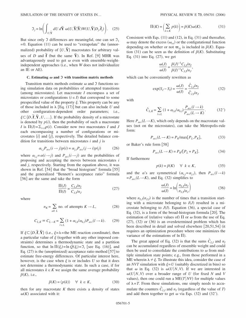
Figure 1 shows the results for the incremental values ofln � obtained for the ME�T V� runs. Clearly � obtained viaEq. �32� ME agrees quantitatively with that obtained with theconventional ME �obtained via the MHR Eq. �24��, althoughthe latter exhibits noticeable larger noise than the former.The improved statistical accuracy in � estimates from TMmethods �like Eq. �32�� relative to those from visited-states


056701-7

methods �like MHR� has been thoroughly quantified before

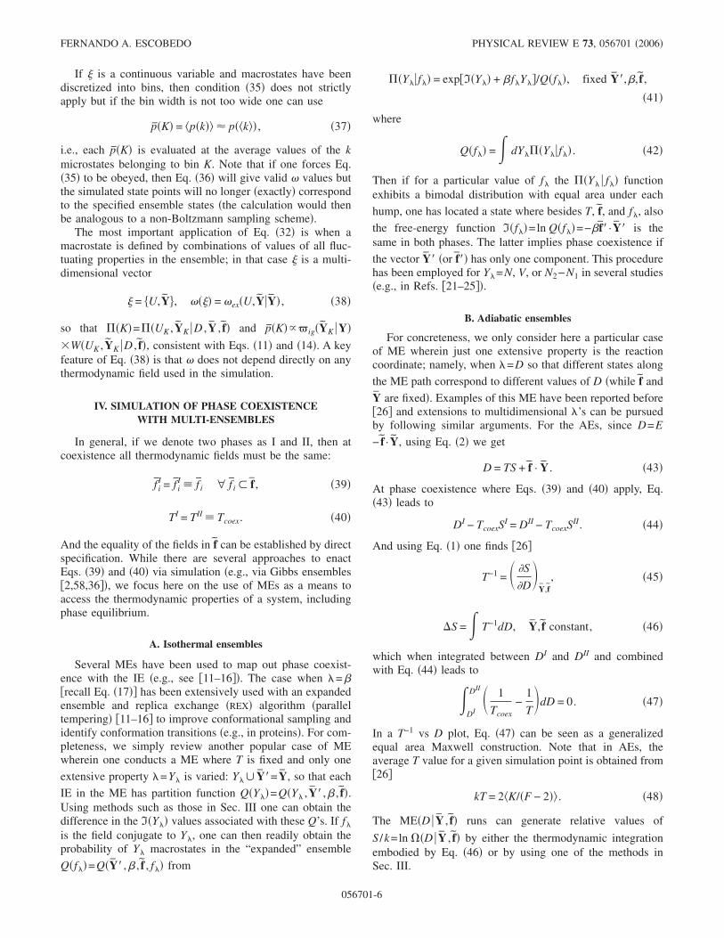
�20,51,54�. The importance of using the appropriate CI,J defi-nition is illustrated by obtaining � via Eq. �36� instead of the“correct” Eq. �32�; clearly, Eq. �36� leads to results exhibit-ing systematic errors. Similar outcomes were obtained whenwe performed the corresponding comparison with data fromadiabatic ME runs �not shown�. Further, the � values ob-tained from isothermal MEs agree completely with thosefrom adiabatic MEs, whether one uses Eq. �32� or Eq. �24��with the latter always exhibiting larger noise�. This agree-ment is illustrated in Fig. 2 where we show that the energyhistograms for several temperatures collected with the stan-dard isothermal MEs, match well those reweighted �e.g.,with Eq. �11�� from the � obtained via Eq. �32� with theadiabatic ME.

The simulations described above were also used to testthe validity of Eq. �19�. Because the results for �

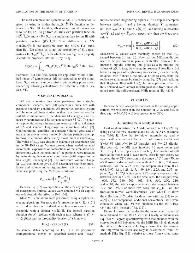
��ex�U V� found before �from either ME series� targeted theU range �−700,−500�, the two integration limits in Eq. �19�pose some limitations: �1� the resulting ��E V� will be ap-proximate because �ex is not known down to U→ �lowerlimit�, and �2� we can only get results for � up to E=−500�upper limit�. In Fig. 3 we plot the results obtained fromthis integration and for I=S /k=ln ��E V� as obtained fromthe use of Eq. �27� for the ME�E V� REX swaps. It can beseen that both sets of data agree well in the overlappingrange of E.

If we are interested in obtaining a “two-dimensional”�2D� ��U ,V� over a broad �U ,V� domain, an economic wayto do so is by assembling several ��U V� isochores, gener-ated for different volumes, via multiple NVE or NVT runs.Such a “multiple 1D paths” approach to � has been illus-trated before �54� wherein the ��U V� isochores were firstfound using an �ensemble-weight-independent�multicanonical-type TM method, and then “stitched” to-gether via a ME�V T� run. Of course, one can use insteadmultiple NVE or NVT ensemble runs to get the ��U V�curves �instead of an ensemble-weight-independent ap-proach�. We tested two such schemes for the N=128 LJ sys-tem, one relying exclusively on IEs and the other on AEs.Since the results from both are comparable, we will onlydescribe the adiabatic scheme wherein we used ME�E V�runs to get the isochoric �’s and stitched them with aME�V E� run. For each volume, we performed the ME�E V�using REX with 28 E values ranging from −600 to +1400�with intervals gradually increasing�, monitored the U rangebetween −806� and 64� discretized in 435 bins ��U=��=2�, and used Eq. �32� to get ��U V�; each ensemble statewas run for 15 000 cycles, where each cycle consisted ofattempting 700 translations and four REX swaps. We simu-lated 40 such isochores for volumes ranging from 129.43to 9878.4 with a nearly logarithmic spacing. For the�stitching� volume-varying ME run, we let V adopt 195discrete values in the same range as before with Vi=127.996 exp�0.022 345�i−0.5�� for i=1,2 , . . . ,195. In thiscase we used a serial ME wherein volume transitions in-volved only two neighbor ensembles at a time �similar to

FIG. 1. �Color online� Density of states function ln ��U V� forthe LJ fluid obtained from ten NVT ensemble runs �for T=0.73,0.84, 0.97, 1.11, 1.28, 1.47, 1.69, 1.94, 2.23, and 2.57� and fixedN=110, V=125. Results are shown for the MHR technique �gray�red� lines�, for the correct TM method �Eq. �32�, full lines�, and forthe “incorrect” TM method �Eq. �36�, dashed lines�.

FIG. 2. Comparison of energy histograms for the LJ fluid ob-tained from standard canonical simulations for temperatures 0.97,1.11, 1.28, 1.47, 1.69, and 1.94 �circles� and by reweighting of the��U V� function obtained from ME�E N ,V� �lines�. The lattercomprised ten runs with E=−600, −572, −540, −505, −465, −418,−360, −290, −210, and −110. In all cases N=110, V=125.

FIG. 3. Comparison of the simulated entropy �ln ��E V�� forthe LJ fluid as obtained from multiple NVE runs �circles� and fromthe integration �via Eq. �19�� of the ��U V� data shown in Fig. 1�lines�.


056701-8

“successive umbrella sampling” �59�� so that in average, ev-ery ensemble point was run for 15 000 cycles, each consist-ing of attempting 200 single-particle translations and eightvolume changes. For this stitching ME, we set E=Es=150and used Eq. �27� to obtain the ratios of successive ��V�values.

The scheme described above also allows us to get ��E ,V�if we collect the �I=�S�E V� values from the REX swaps�isochoric runs�. The stitching can be done by using

S�E,V� = S�EV� + �S�VEs� − S�V0Es��

− �S�EsV� − S�EsV0�� 53�

where V0 is an arbitrary volume used as reference, and theterms in the first square brackets are from the ME�V Es� runwhile all the others in the right hand side of Eq. �53� arefrom the ME�E V� runs. To get S�U ,V�=k ln ��U ,V�, it canbe shown that the stitching can be done with

S�U,V� = S�UV� + �S�VEs� − S�V0Es��

− �S� �EsV� − S� �EsV0�� 54�

where the S� terms are found by integration of the simulated

��U V�=exp�S�U V�� data �from the ME�E V� run� via Eq.�19�; i.e.,

S� �EsV� = ln ��EsV� = ln� −

Es

dU��U�V��Es − U��F/2−1� .

�55�

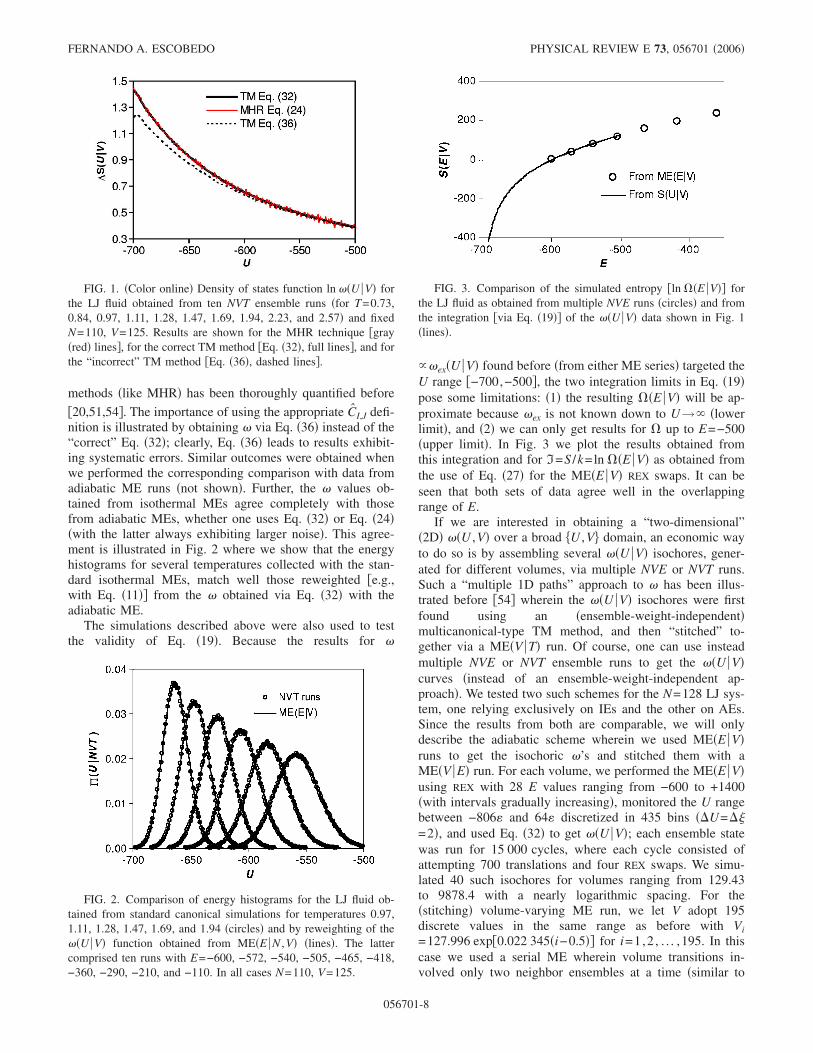
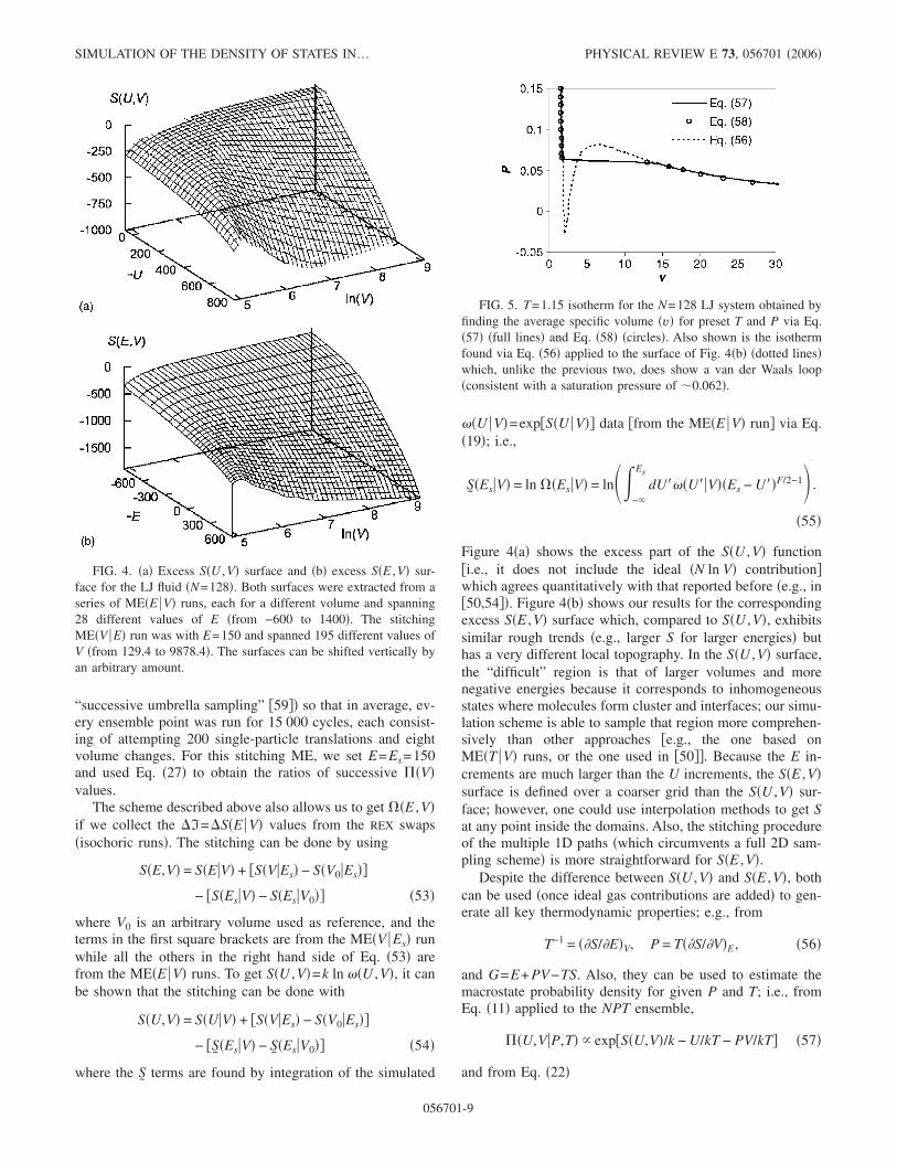
Figure 4�a� shows the excess part of the S�U ,V� function�i.e., it does not include the ideal �N ln V� contribution�which agrees quantitatively with that reported before �e.g., in�50,54��. Figure 4�b� shows our results for the correspondingexcess S�E ,V� surface which, compared to S�U ,V�, exhibitssimilar rough trends �e.g., larger S for larger energies� buthas a very different local topography. In the S�U ,V� surface,the “difficult” region is that of larger volumes and morenegative energies because it corresponds to inhomogeneousstates where molecules form cluster and interfaces; our simu-lation scheme is able to sample that region more comprehen-sively than other approaches �e.g., the one based onME�T V� runs, or the one used in �50��. Because the E in-crements are much larger than the U increments, the S�E ,V�surface is defined over a coarser grid than the S�U ,V� sur-face; however, one could use interpolation methods to get Sat any point inside the domains. Also, the stitching procedureof the multiple 1D paths �which circumvents a full 2D sam-pling scheme� is more straightforward for S�E ,V�.

Despite the difference between S�U ,V� and S�E ,V�, bothcan be used �once ideal gas contributions are added� to gen-erate all key thermodynamic properties; e.g., from

T−1 = ��S/�E�V, P = T��S/�V�E, �56�

and G=E+ PV−TS. Also, they can be used to estimate themacrostate probability density for given P and T; i.e., fromEq. �11� applied to the NPT ensemble,

��U,VP,T� � exp�S�U,V�/k − U/kT − PV/kT� �57�

and from Eq. �22�

FIG. 4. �a� Excess S�U ,V� surface and �b� excess S�E ,V� sur-face for the LJ fluid �N=128�. Both surfaces were extracted from aseries of ME�E V� runs, each for a different volume and spanning28 different values of E �from −600 to 1400�. The stitchingME�V E� run was with E=150 and spanned 195 different values ofV �from 129.4 to 9878.4�. The surfaces can be shifted vertically byan arbitrary amount.

FIG. 5. T=1.15 isotherm for the N=128 LJ system obtained byfinding the average specific volume �v� for preset T and P via Eq.�57� �full lines� and Eq. �58� �circles�. Also shown is the isothermfound via Eq. �56� applied to the surface of Fig. 4�b� �dotted lines�which, unlike the previous two, does show a van der Waals loop�consistent with a saturation pressure of �0.062�.


056701-9

��E,VP,T� � exp�S�E,V�/k − E/kT − PV/kT� �58�

with which average properties �X�=X��U ,V�dU dV and�X�=X��E ,V�dE dV can be found. Figure 5 shows PV datafor a subcritical isotherm found using Eqs. �56�–�58�. Al-though phase coexistence could be estimated from such iso-therms, Eqs. �57� and �58� allow a more direct route via the“equal-probability-volume” criterion wherein one finds P-Tpairs of values that give a bimodal probability density havingequal “volume” �total probability� under each peak. Unre-ported sample coexistence results using Eqs. �57� and �58��see, however, Fig. 6�b�� agree with each other and withthose given in Ref. �50�. Note that ��U+K ,V P ,T� from Eq.�57� with K=3NkT /2 �a maximum term approximation� isnot the same as ��E ,V P ,T� from Eq. �58� since the formerdoes not capture the variability of K.

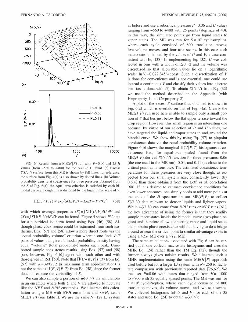
We can also sample a portion of ��U ,V� via simulationsin an ensemble where both U and V are allowed to fluctuatelike the NPT and NPH ensembles. We illustrate this calcu-lation using a ME with NPH ensembles and �=H, i.e., aME�H P� �see Table I�. We use the same N=128 LJ system

as before and use a subcritical pressure P=0.06 and H valuesranging from −560 to +400 with 25 points �step size of 40�;in this way, the simulated points go from liquid states tovapor states. The ME was run for 5�104 cycles/replica,where each cycle consisted of 800 translation moves,five volume moves, and four REX swaps. In this case eachmacrostate is defined by the values of U and V, a case con-sistent with Eq. �38�. In implementing Eq. �32�, U was col-lected in bins with a width of �U=2 and the volume wasdiscretized so that allowable values lie on a logarithmicscale: ln Vi=0.022 345i+const. Such a discretization of Vis done for convenience and is not essential; one could useinstead a continuous V and classify their values into discretebins �as is done with U�. To obtain S�U ,V� from Eq. �32�we used the method described in the Appendix �withV=property 1 and U=property 2�.

A plot of the excess S surface thus obtained is shown inFig. 6�a� which is overlaid on that of Fig. 4�a�. Clearly theME�H P� run used here is able to sample only a small por-tion of S that lies just below the flat upper terrace toward thedrop region. However, this small region is an interesting onebecause, by virtue of our selection of P and H values, wehave targeted the liquid and vapor states in and around thebinodal curve. We show this by using Eq. �57� to pinpointcoexistence data via the equal-probability-volume criterion.Figure 6�b� shows the marginal ��V P ,T� histograms at co-existence �i.e., for equal-area peaks� found from theME�H P�-derived S�U ,V� function for three pressures: 0.06�the one used in the ME run�, 0.04, and 0.11 �as close to thecritical point as is sensible�. The estimated coexistence tem-peratures for these pressures are very close though, as ex-pected from our small system size, consistently lower �by0.6%� than those obtained from the Lotfi et al. correlation�60�. If it is desired to estimate coexistence conditions foreven lower pressures, one simply needs to add more points atthe ends of the H spectrum in our ME�H P� to collectS�U ,V� data relevant to denser liquids and lighter vapors.While ��U ,V� can come from NPH runs or NPT runs �61�,the key advantage of using the former is that they readilysample macrostates inside the bimodal curve �two-phase re-gion� and therefore allow connecting vapor and liquid statesand pinpoint phase coexistence without having to do a bridgearound or near the critical point �a similar advantage exists inusing a VL� ME over a VT� ME�.

The same calculations associated with Fig. 6 can be car-ried out if one collects macrostate histograms and uses theMHR Eq. �24� rather than the TM Eq. �32�, though theformer always gives noisier results. We illustrate such aMHR implementation using the same ME�H P� approachused before but for a larger LJ system with N=250 to facili-tate comparison with previously reported data �26,62�. Wethus set P=0.06 with states that ranged from H=−1000to +700 with 35 equally spaced points. The ME was run for5�104 cycles/replica, where each cycle consisted of 800translation moves, six volume moves, and two REX swaps.We collected histograms �of U and V� for each of the 35states and used Eq. �24� to obtain ��U ,V�:

FIG. 6. Results from a ME�H P� run with P=0.06 and 25 Hvalues �from −560 to +400� for the N=128 LJ fluid. �a� ExcessS�U ,V� surface from this ME is shown by full lines; for reference,the surface from Fig. 4�a� is also shown by dotted lines. �b� Volumeprobability density at coexistence for three pressures obtained fromthe S of Fig. 6�a�; the equal-area criterion is satisfied by each bi-modal curve although this is distorted by the logarithmic scale of V.


056701-10

��U,V� =� j=1

s H�U,VHj,Pj�

� j=1

s K jW�U,VHj,Pj�exp�− Sj/k�, �24��

where W is given in Table I, and Sj is the �relative� entropyof the jth state �found from either Eq. �25� or from Bennett’sEq. �27� applied to the REX swaps�. We then obtained theprobability density of macrostates at other conditions of Hand P, from

��U,VH,P� � ��U,V�W�U,VH,P� , �11��

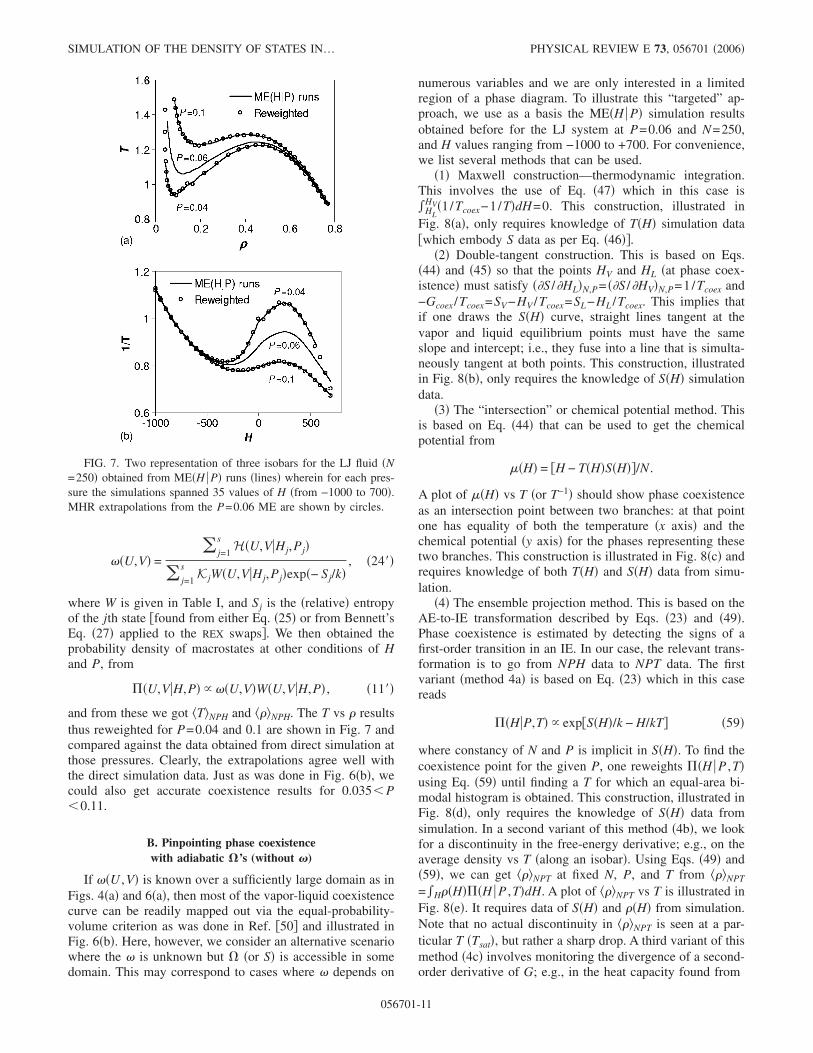
and from these we got �T�NPH and ��NPH. The T vs � resultsthus reweighted for P=0.04 and 0.1 are shown in Fig. 7 andcompared against the data obtained from direct simulation atthose pressures. Clearly, the extrapolations agree well withthe direct simulation data. Just as was done in Fig. 6�b�, wecould also get accurate coexistence results for 0.035� P�0.11.

B. Pinpointing phase coexistencewith adiabatic �’s (without �)

If ��U ,V� is known over a sufficiently large domain as inFigs. 4�a� and 6�a�, then most of the vapor-liquid coexistencecurve can be readily mapped out via the equal-probability-volume criterion as was done in Ref. �50� and illustrated inFig. 6�b�. Here, however, we consider an alternative scenariowhere the � is unknown but � �or S� is accessible in somedomain. This may correspond to cases where � depends on

numerous variables and we are only interested in a limitedregion of a phase diagram. To illustrate this “targeted” ap-proach, we use as a basis the ME�H P� simulation resultsobtained before for the LJ system at P=0.06 and N=250,and H values ranging from −1000 to +700. For convenience,we list several methods that can be used.

�1� Maxwell construction—thermodynamic integration.This involves the use of Eq. �47� which in this case isHL

HV�1/Tcoex−1/T�dH=0. This construction, illustrated inFig. 8�a�, only requires knowledge of T�H� simulation data�which embody S data as per Eq. �46��.

�2� Double-tangent construction. This is based on Eqs.�44� and �45� so that the points HV and HL �at phase coex-istence� must satisfy ��S /�HL�N,P= ��S /�HV�N,P=1/Tcoex and−Gcoex /Tcoex=SV−HV /Tcoex=SL−HL /Tcoex. This implies thatif one draws the S�H� curve, straight lines tangent at thevapor and liquid equilibrium points must have the sameslope and intercept; i.e., they fuse into a line that is simulta-neously tangent at both points. This construction, illustratedin Fig. 8�b�, only requires the knowledge of S�H� simulationdata.

�3� The “intersection” or chemical potential method. Thisis based on Eq. �44� that can be used to get the chemicalpotential from

��H� = �H − T�H�S�H��/N .

A plot of ��H� vs T �or T−1� should show phase coexistenceas an intersection point between two branches: at that pointone has equality of both the temperature �x axis� and thechemical potential �y axis� for the phases representing thesetwo branches. This construction is illustrated in Fig. 8�c� andrequires knowledge of both T�H� and S�H� data from simu-lation.

�4� The ensemble projection method. This is based on theAE-to-IE transformation described by Eqs. �23� and �49�.Phase coexistence is estimated by detecting the signs of afirst-order transition in an IE. In our case, the relevant trans-formation is to go from NPH data to NPT data. The firstvariant �method 4a� is based on Eq. �23� which in this casereads

��HP,T� � exp�S�H�/k − H/kT� �59�

where constancy of N and P is implicit in S�H�. To find thecoexistence point for the given P, one reweights ��H P ,T�using Eq. �59� until finding a T for which an equal-area bi-modal histogram is obtained. This construction, illustrated inFig. 8�d�, only requires the knowledge of S�H� data fromsimulation. In a second variant of this method �4b�, we lookfor a discontinuity in the free-energy derivative; e.g., on theaverage density vs T �along an isobar�. Using Eqs. �49� and�59�, we can get ��NPT at fixed N, P, and T from ��NPT

=H��H��H P ,T�dH. A plot of ��NPT vs T is illustrated inFig. 8�e�. It requires data of S�H� and ��H� from simulation.Note that no actual discontinuity in ��NPT is seen at a par-ticular T �Tsat�, but rather a sharp drop. A third variant of thismethod �4c� involves monitoring the divergence of a second-order derivative of G; e.g., in the heat capacity found from

FIG. 7. Two representation of three isobars for the LJ fluid �N=250� obtained from ME�H P� runs �lines� wherein for each pres-sure the simulations spanned 35 values of H �from −1000 to 700�.MHR extrapolations from the P=0.06 ME are shown by circles.


056701-11

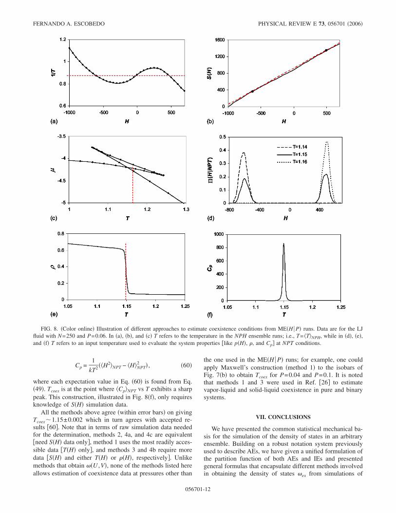
Cp =1

kT2 ��H2�NPT − �H�NPT2 � , �60�

where each expectation value in Eq. �60� is found from Eq.�49�. Tcoex is at the point where �Cp�NPT vs T exhibits a sharppeak. This construction, illustrated in Fig. 8�f�, only requiresknowledge of S�H� simulation data.

All the methods above agree �within error bars� on givingTcoex�1.15±0.002 which in turn agrees with accepted re-sults �60�. Note that in terms of raw simulation data neededfor the determination, methods 2, 4a, and 4c are equivalent�need S�H� data only�, method 1 uses the most readily acces-sible data �T�H� only�, and methods 3 and 4b require moredata �S�H� and either T�H� or ��H�, respectively�. Unlikemethods that obtain ��U ,V�, none of the methods listed hereallows estimation of coexistence data at pressures other than

the one used in the ME�H P� runs; for example, one couldapply Maxwell’s construction �method 1� to the isobars ofFig. 7�b� to obtain Tcoex for P=0.04 and P=0.1. It is notedthat methods 1 and 3 were used in Ref. �26� to estimatevapor-liquid and solid-liquid coexistence in pure and binarysystems.

VII. CONCLUSIONS

We have presented the common statistical mechanical ba-sis for the simulation of the density of states in an arbitraryensemble. Building on a robust notation system previouslyused to describe AEs, we have given a unified formulation ofthe partition function of both AEs and IEs and presentedgeneral formulas that encapsulate different methods involvedin obtaining the density of states �ex from simulations of

FIG. 8. �Color online� Illustration of different approaches to estimate coexistence conditions from ME�H P� runs. Data are for the LJfluid with N=250 and P=0.06. In �a�, �b�, and �c� T refers to the temperature in the NPH ensemble runs; i.e., T= �T�NPH, while in �d�, �e�,and �f� T refers to an input temperature used to evaluate the system properties �like p�H�, �, and Cp� at NPT conditions.


056701-12

AEs and IEs. Once �ex is obtained, whether it was fromIE or AE runs, we showed that one can reweight �exvia Eq. �11� to obtain probability densities and other pro-perties for the suitable ensemble. For example one couldgo from NVT �multi�ensemble data→�ex�U N ,V�→NVEensemble data, or vice versa; i.e., from NVE �multi�ensembledata→�ex�U N ,V�→NVT ensemble data.

Using the Lennard-Jones system as a testbed, we haveapplied and compared the calculation of � based on MHR �avisited-states method� and a TM scheme �a transition prob-ability method�. We found that the latter generates resultswith less statistical noise than the former, an advantage thathas been associated with TM methods before and is expectedto hold for more complex systems. We have also shown thatby a suitable generalization of the acceptance-ratio methodone arrives at a simple formula �Eq. �32�� that allows theinformation on microstate transitions from different simula-tion points to be simply added to global counters. In thisway, the TM route to � is not only more accurate than theMHR route but it provides a convenient bookkeepingscheme to consolidate all the statistical data needed to get �.

Unlike multiple NPT runs �for varying T�, the use of mul-tiple NPH runs �for varying H� allows one to bridge twocoexistence phases for any P. This leads to the collection ofa more complete � function for the reweighting of data overa broad range of T and P; in particular, to obtain vapor-liquidcoexistence data over a wide pressure range. Finally, we il-lustrated the use of different approaches to pinpoint vapor-liquid coexistence in the LJ fluid from the information ofmultiple NPH runs at constant pressure. Such methods arenot confined to the NPH ensemble nor to pure componentsand could be especially valuable in cases where insertion ordeletion of particles is troublesome �e.g., for large or cyclicmolecules�.

It is expected that the IE↔�ex↔AE connection will helpidentify instances where one can harness the strengths of AIsand AEs. Generating S�E ,V� rather than S�U ,V�, for ex-ample, may be advantageous in some cases. While we fo-cused on mapping S�U ,V� and S�E ,V�, similar approachescan be used to map S�U ,N� and S�E ,N�. For convenience,we have employed the simplest possible systems to validatethe advocated methods. Some algorithmic refinements maybe needed to simulate systems with more components orwith macrostates defined by structure-dependent order pa-rameters. For example, within the framework of REX andBennett’s acceptance-ratio methods, data from virtual swapmoves could be used to optimize the estimation of the J or �function as was done in Ref. �63�.

ACKNOWLEDGMENTS

Support is acknowledged from the Sloan Foundation andfrom the National Science Foundation, Grant No. BES-0093769.

APPENDIX: IMPLEMENTATION OF EQ. (32)FOR A 2D DOMAIN

The determination of S differences from Eq. �32� is anoverdetermined problem because for any macrostates I and

J, SJ−SI can be found not only from the direct transitionsbetween I and J but also from the results of other jumps; i.e.,via any path that starts at I and ends at J in more than 1 step.The solution to the problem of finding “optimal” S differ-ences has been described before for cases when a “mac-rostate” is defined by the values of a single macrovariable�20,51,54�. It involves the minimization of the total varianceof the estimation of S differences via a least-squares analysis.In principle, the same procedure can be used when each mac-rostate is defined by two or more macrovariables but the sizeof the arrays can become very large and cumbersome tohandle. We describe here an alternative procedure for a casewith two macrovariables that takes advantage of the fact thatfor one of the macrovariables, denoted here “property 1,”transitions can at most take the system between macrostateshaving neighboring values of such a property. Property 1could be for instance V or any other property �like N� whosevalues �and transition between them� can be directly speci-fied. On the other hand, “property 2” is a macrovariable likeU for which transition end points cannot be directly specified�due to its coupling with the system configuration�.

Every macrostate can then be specified by two indexes so

that the terms C and n in Eq. �32� are denoted C�i ,�i , j ,k�and n�i ,�i , j� where the index i gives the current state ofproperty 1, and �i gives its change as a result of by theproposed transition; �i= ±1 if a change in property 1 isproposed and �i=0 otherwise. The indices j and k denotethe current and new values of property 2, respectively.The entropy change associated with any transition �i , j�→ �i+�i ,k� is therefore denoted as S�i+�i ,k�−S�i , j�. In-stead of solving for all the optimal S values at once, weadopted the following two-step process.

�1� Find first the optimal S�i ,k�−S�i , j� values, i.e., forevery “slice” of macrophase space with fixed value of prop-erty 1. For each value of i �and with �i=0�, this involves thesolution of a 1D problem for the �i , j�→ �i ,k� transitionswhich is identical to previous applications of the optimiza-tion method and to the one we used to get S in Fig. 1 �whereV was fixed and only transitions between U macrostates wereconsidered�. In the present case Eq. �32� takes the form

S�i,k� − S�i, j� = ln� C�i,0, j,k�/n�i,0, j�

C�i,0,k, j�/n�i,0,k�� . �A1�

The redundancy in the information on �i , j�→ �i ,k� transi-tions was used to estimate optimal S*�i ,k�−S*�i , j� values asreported in Ref. �54� �the asterisks are used to denote optimalS values found in this step�.

�2� Find the relative shifts �S between successive S slicesfound in step 1; i.e.,

�Si+1 = Sopt�i + 1,k� − Sopt�i,k�

− �S*�i + 1,k� − S*�i,k�� " k . �A2�

In other words, �Si+1 is the quantity that we need to add toSopt�i ,k� to get the best value for the next slice Sopt�i+1,k�.Note that the differences �S*�i+1,k�−S*�i ,k�� obtained fromstep 1 are arbitrary. Meaningful estimates for �S�i+1,k�−S�i ,k�� can be obtained from transitions that involved


056701-13

changes of property 1 �only� between values i and i+1; thesecan be estimated using Eq. �32�:

�Sj,k = S�i + 1,k� − S�i, j�

= ln� C�i, + 1, j,k�/n�i, + 1, j�

C�i + 1,− 1,k, j�/n�i + 1,− 1,k�� . �A3�

Thus estimates for the �S shift can be found from

�Si+1 = �Sj,k − �Sj,k*

where �Sj,k is from Eq. �A3� and �Sj,k* =S*�i+1,k�−S*�i , j�.

Since �S must be the same regardless of the values of prop-erty 2 �i.e., for any j and k values�, we can find the optimalshift �Si+1

opt by minimizing the total variance given by

�i,tot2 = �

j,k

��Si+1opt − ��Sj,k − �Sj,k

* ��2

� j,k2 �A4�

where

� j,k2 = 1/C�i, + 1, j,k� + 1/C�i + 1,− 1,k, j�

+ 1/n�i, + 1, j� + 1/n�i + 1,− 1,k� . �A5�

Setting d�i,tot2 /d��Si+1

opt�=0 we find the sought-after solution:

�Si+1opt = �

j,k

��Sj,k − �Sj,k* �

� j,k2 ��

j,k

1

� j,k2 . �A6�

Once �Si+1opt is found, one then uses Eq. �A2� to find the op-

timal values for Sopt�i+1,k� for all k values, and going se-quentially from i=2,3 , . . ., having set Sopt�1,k�=S*�1,k�.Note that in some respects, this two-step procedure is remi-niscent of the multiple 1D paths+stitching approach de-scribed in Sec. VI �regarding Fig. 4�, except that here the MErun involved 2D transitions so that the information for thestitching �step 2 here� does not require a separate run. Thistwo-step process is not restricted to ME runs but can also beapplied to ensemble-weight-independent multicanonical-typesimulations and generalized for more than two macrovariables.

�1� M. P. Allen and D. J. Tildesley, Computer Simulation ofLiquids �Clarendon Press, Oxford, 1987�.

�2� D. Frenkel and B. Smit, Understanding Molecular Simulation:From Algorithms to Applications �Academic, San Diego,2000�.

�3� A. M. Ferrenberg and R. H. Swendsen, Phys. Rev. Lett. 61,2635 �1988�.

�4� A. M. Ferrenberg and R. H. Swendsen, Phys. Rev. Lett. 63,1195 �1989�; P. Labastie and R. L. Whetten, ibid. 65, 1567�1990�.

�5� N. B. Wilding, Phys. Rev. E 52, 602 �1995�.�6� A. Z. Panagiotopoulos, J. Phys.: Condens. Matter 12, R25

�2000�.�7� J. J. de Pablo, Q. Yan, and F. A. Escobedo, Annu. Rev. Phys.

Chem. 50, 377 �1999�.�8� A. D. Bruce and N. B. Wilding, Adv. Chem. Phys. 127, 1

�2003�.�9� C. H. Abreu and F. A. Escobedo, J. Chem. Phys. 124, 054116

�2006�.�10� C. Bartels, M. Schaefer, and M. Karplus, J. Chem. Phys. 111,

8048 �1999�.�11� P. Lyubartsev, A. A. Martinovski, S. V. Shevkunov, and P. N.

Vorontsov Velyaminov, J. Chem. Phys. 96, 1776 �1992�.�12� N. B. Wilding and M. Muller, J. Chem. Phys. 101, 4324

�1994�.�13� F. A. Escobedo and J. J. de Pablo, J. Chem. Phys. 103, 2703

�1995�.�14� M. C. Tesi, E. J. J. van Rensburg, E. Orlandini, and S. G.

Whittington, J. Stat. Phys. 82, 155 �1996�.�15� U. H. E. Hansmann, Chem. Phys. Lett. 281, 140 �1997�.�16� Q. Yan and J. J. de Pablo, J. Chem. Phys. 111, 9509 �1999�;

113, 1276 �2000�.�17� M. Fitzgerald, R. R. Picard, and R. N. Silver, Europhys. Lett.

46, 282 �1999�.�18� M. Fitzgerald, R. R. Picard, and R. N. Silver, J. Stat. Phys. 98,

321 �2000�.�19� G. R. Smith and A. D. Bruce, J. Phys. A 28, 6623 �1995�.�20� J.-S. Wang and R. H. Swendsen, J. Stat. Phys. 106, 245

�2002�.�21� J. R. Errington, Phys. Rev. E 67, 012102 �2003�.�22� J. R. Errington, J. Chem. Phys. 118, 9915 �2003�.�23� M. K. Fenwick and F. A. Escobedo, J. Chem. Phys. 119,

11998 �2003�.�24� M. K. Fenwick and F. A. Escobedo, J. Chem. Phys. 120, 3066

�2004�.�25� I. D. Gospodinov and F. A. Escobedo, J. Chem. Phys. 122,

164103 �2005�.�26� F. Escobedo, J. Chem. Phys. 123, 044110 �2005�.�27� H. W. Graben and J. R. Ray, Phys. Rev. A 43, 4100 �1991�.�28� H. W. Graben and J. R. Ray, Mol. Phys. 80, 1183 �1993�.�29� M. Parrinello and A. Rahman, Phys. Rev. Lett. 45, 1196

�1980�.�30� J. R. Ray and H. W. Graben, J. Chem. Phys. 75, 4077 �1981�.�31� J. R. Ray, Phys. Rev. A 44, 4061 �1991�.�32� J. R. Ray and H. W. Graben, J. Chem. Phys. 93, 4296 �1990�.�33� R. Lustig, J. Chem. Phys. 109, 8816 �1998�.�34� Z. Zhou, J. Chem. Phys. 114, 8769 �2001�.�35� T. Kristof and J. Liszi, Chem. Phys. Lett. 261, 620 �1996�.�36� T. Kristof and J. Liszi, Mol. Phys. 94, 519 �1998�.�37� L. Merenyi and T. Kristof, Mol. Phys. 30, 549 �2004�.�38� F. Calvo and P. Labastie, Chem. Phys. Lett. 247, 395 �1995�.�39� F. Calvo and P. Labastie, Eur. Phys. J. D 3, 229 �1998�.�40� F. Calvo, J. P. Neirotti, D. L. Freeman, and J. D. Doll, J. Chem.

Phys. 112, 10350 �2000�.�41� F. Calvo, Mol. Phys. 100, 3421 �2002�.�42� L. I. Kioupis, G. Arya, and E. J. Maginn, Fluid Phase Equilib.

200, 93 �2002�.�43� B. A. Berg and T. Neuhaus, Phys. Rev. Lett. 68, 9 �1992�.�44� B. A. Berg and T. Celik, Phys. Rev. Lett. 69, 2292 �1992�.�45� J. Lee, Phys. Rev. Lett. 71, 211 �1993�; 71, 2353 �1993�.


056701-14

�46� F. Wang and D. P. Landau, Phys. Rev. Lett. 86, 2050 �2001�.�47� F. Wang and D. P. Landau, Phys. Rev. E 64, 056101 �2001�.�48� Q. Yan, R. Faller, and J. J. de Pablo, J. Chem. Phys. 116, 8745

�2002�.�49� Q. Yan and J. J. de Pablo, Phys. Rev. Lett. 90, 035701 �2003�.�50� M. S. Shell, P. G. Debenedetti, and A. Z. Panagiotopoulos,

Phys. Rev. E 66, 056703 �2002�.�51� M. S. Shell, P. G. Debenedetti, and A. Z. Panagiotopoulos, J.

Chem. Phys. 119, 9406 �2003�.�52� F. A. Escobedo, J. Chem. Phys. 15, 5642 �2001�.�53� W. H. Press, W. T. Vetterling, S. A. Teukolsky, and B. P. Flan-

nery, Numerical Recipes in Fortran 77: The Art of ScientificComputing, 2nd ed. �Cambridge University Press, New York,2001�, p. 786.

�54� F. A. Escobedo and C. H. Abreu, J. Chem. Phys. 124, 104110

�2006�.�55� P. M. C. de Oliveira, T. J. P. Penna, and H. J. Herrmann, Braz.

J. Phys. 26, 677 �1996�.�56� C. H. Bennett, J. Comput. Phys. 22, 245 �1976�.�57� A. A. Barker, Aust. J. Phys. 18, 119 �1965�.�58� A. Z. Panagiotopoulos, Mol. Phys. 61, 813 �1987�.�59� P. Virnau and M. Muller, J. Chem. Phys. 120, 10925 �2004�.�60� A. Lofti, J. Vrabec, and J. Fischer, Mol. Phys. 76, 1319

�1992�.�61� P. B. Conrad and J. J. de Pablo, Fluid Phase Equilib. 150, 51

�1998�.�62� In Ref. �26�, the data for P=0.02 in Figs. 4 and 5 are for a

system with 200 �not 250� particles.�63� I. Coluzza and D. Frenkel, ChemPhysChem 6, 1779 �2005�.


056701-15

Documents

Simulation of the density of states in isothermal and adiabatic ensembles