Simulation of spatial and temporal variations of dissolved oxygen …€¦ · Simulation of spatial and temporal variations of dissolved oxygen of Baynespruit stream in South Africa

Simulation of spatial and temporal variations of dissolved oxygen of Baynespruit stream in South Africa

Muthukrishnavellaisamy Kumarasamy School of Civil Engineering Surveying and Construction, University of KwaZulu-Natal, Durban, South Africa

Abstract

Water is essential for life processes of all species in the environment and for the socio-economic development of the human community. Without proper water quality, the life sustainability of many species is definitely doubtful. Pollutants from various sources enter river systems and cause serious river water pollution. In this situation, we need to understand how pollutants are transported along the water course, the types and sources of these pollutants and their effects on water quality. By understanding the water pollution and self-cleaning capacity of a river system, one can make an appropriate decision for managing pollutant disposal. While a non-conservative pollutant enters a water course, depletion of dissolved oxygen (DO) takes place due to the consumption of oxygen in addition to advection and dispersion. At the same time, depending on the deficit of DO, re-aeration process takes place at a specific rate. There are many ways to solve DO and non-conservative pollutant relationships, such as the Streeter–Phelps model, many other concepts and experimental studies. The limitations of the previous studies on DO are that they are primarily based on the advection principle and first order decay only. In this study, considering first order decay along with advection and dispersion, DO concentration has been simulated by making use of mathematical mixing cells model incorporating de-oxygenation and re-aeration. In order for the validation, the results of the proposed model are compared with that of advection-dispersion based DO model. The spatial and temporal distribution of dissolved oxygen concentrations of Baynespruit stream in South Africa has been simulated having some input data and compared with large set of dissolved oxygen data at various locations of the stream. Keywords: dissolved oxygen, mixing cells concept, Baynespruit stream.

Water Resources Management VI 403

www.witpress.com, ISSN 1743-3541 (on-line) WIT Transactions on Ecology and the Environment, Vol 145, © 2011 WIT Press

doi:10.2495/WRM110351

1 Introduction

Water is the most valuable resource that we have on Earth and it is required to sustain essential life processes for all species and organisms in the world, for social development and economic progress for humans. Water is the most abundant liquid around the world, but the quantity of water that is potable (drinkable) is less than three percent of all surface water on Earth. Storm water is often drained into nearby streams and rivers or the treated effluents from wastewater treatment plants are passed through a stream or river so as to increase the properties of the treated water. Pollutants, that enter streams or rivers without proper treatment, cause pollution of the respective system and river water quality deteriorates. These external pollutants pose a great threat to the quality of water. Water pollution is the main cause of poor water quality around the world. Thus we need to understand the sources of these pollutants, how pollutants are transported to a water system, and how they affect the quality of the water. This study on pollutant transport will lead to advanced pollution control and appropriate decision making for the management of pollution effluents and availability of potable water. Typical pollutants that are found are classed into Physical, Chemical and Biological pollutants. This study focuses on non-conservative pollutant transport and dissolved oxygen concentration which are main water quality parameters in assessing water quality status of rivers. The pollutants most commonly associated with decay are: effluents from wastewater treatment plants (Biological Oxygen Demand and sludge), human and animal faeces, and chemicals from household and industrial use, fertilizers and pesticides from agricultural use. These non-conservative pollutants are generated by: urban runoff, failing septic systems, straight pipes, agriculture, forestry, mining, and construction and stream projects. Water quality problems that arise from these non-conservative pollutants and pollutant sources are odour, increase in pathogens into a stream, destruction of the aquatic environment and the decrease in the availability of oxygen that is naturally present in streams. The key characteristic of non-conservative pollutants in the process of decay is that the oxygen is used as energy to break down the pollutant. Many authors, [3, 19, 20, 28], stated that measuring dissolved oxygen is the most significant water quality test to determine the suitability of a stream. According to Cox [10], the major DO sources (i.e. the areas in which oxygen is introduced into the river or stream) include aeration due to the atmospheric interaction with the water surface; wind and wave action; photosynthesis and human activities. These human activities, which is not a natural phenomena in comparison to the other typical sources comprise of structural elements such as weirs, dams and constructed tributaries. On the other hand, the major causes of ‘oxygen depletion’ are due to respiration of aquatic plants; certain chemicals and the decay of organic material and ‘other reduced matter’ in the water column [10]. The depletion of oxygen that interests us is due to decay of pollutants. A readily available bacterium in the water requires oxygen to break down the particles of pollutants. The rise in DO concentration as the increase in length is due to re-aeration after equilibrium is reached between the pollutant concentration and the

404 Water Resources Management VI


DO concentration. Re-aeration could be due to turbulence of the stream or due to the atmospheric interaction of the water as discussed by Cox [10]. As we have seen, the impacts of water quality from the interaction of non-conservative pollutants and dissolved oxygen is of vital importance to man and more importantly to all living species. There are various ways to solve DO and non-conservative pollutant relationships, such as the Streeter–Phelps model, other models, experiments and computer programs. A rather interesting phenomenon does exist however, in which non-conservative pollutants has a relationship with the amount of Dissolved Oxygen in a water body [26]. The Streeter–Phelps model was a ground breaking approach to evaluate the relationship between constant pollutant loading and resulting sag of the dissolved oxygen (DO) concentration in the downstream water. It can be seen by the Streeter–Phelps model equation and agreed upon by other authors [3, 17] that Streeter and Phelps employed their equations in the form of a first-order partial differential equation model under steady-state conditions, with two processes only, viz. the re-aeration of the stream and the consumption of DO in the oxidation (decay) of BOD (biological oxygen demand). This was expanded upon by Beck and Young [3], in that the implications of suggesting a steady-state model for the description of DO-BOD interaction are based on the assumptions that the concentrations of DO and BOD and the flow rate are “time-invariant” at all points along the longitudinal reach of the river. This assumption of time-invariance conditions such as quantities governing the system’s behaviour remains constant with time is by ‘no means a reasonable assumption’ [3], as the inputs to the model are time-invariant. This is due to the time dependency of the DO and BOD concentrations. The Streeter–Phelps model, however, did break the mould for the study of water quality with regard to DO-BOD interaction models. Over the years from 1925, models which incorporated the basic ideology of the Streeter–Phelps model, achieved better results and understanding due to the model. Many investigators, [3, 12–15, 17, 21], have adapted the Streeter–Phelps model in various ways by adding different parameters and applying different mathematical approaches but fundamentally using the same basic principles of first order kinetics and dissolved oxygen sag. The limitations to the Streeter–Phelps models are that they are primarily based on the advection principle. The limitations of having no dispersion have shown that the models are not as accurate to the reality [1, 4, 5, 9, 11, 16, 25]. After Streeter and Phelps, several concepts were introduced [2, 6–8, 18, 27]. All these approaches assumed that the substances, present in the water, decay according to a first order reaction, i.e., the rate of loss of the substance is proportional to its concentration at any time. Young and Beck [30] proposed continuously stirred tank reactor (CSTR) by joining assumptions of hydrology and chemical engineering to account the BOD-DO reactions and the dispersion in the channel. Rinaldi et al. [23] defined the auxiliary variable which relates the dissolved oxygen deficit and BOD load to get the solution for the approximated Streeter–Phelps dispersion model. In this paper, considering first order decay along with advection and dispersion, DO concentration has been simulated by making use of mixing cells model incorporating de-



oxygenation and re-aeration. The model will also analyse the parameters associated with dissolved oxygen and decaying pollutants with respect to advection, dispersion, decay and re-aeration with spatial and temporal boundaries. The understanding of pollutant transport and the properties of dissolved oxygen are also the basis for formulation of the models so as to determine reasonable water quality results. Ordinary differential equations describe the pollutant and DO mass balance in a series of mixing cells into which the flow domain is discretized. Many authors formulated similar type of models namely compartment model [29], box model, and tanks-in-series model [22, 24]. Mixing-cell models have been used extensively for water quality modeling and chemical engineering applications. The reasons for using mixing cells model are such as 1) it is very simple model which uses 1st order ODE instead 2nd order PDE, 2) it has only one time parameter which can be determined by having flow velocity and the size of mixing unit and 3) it is capable of incorporating any processes of pollutant transport. In this study, it has been aimed to use mixing cells concept to simulate advection, dispersion, decay and re-aeration processes by solving equations for one mixing cell and using discrete kernel co-efficient. Having the pollutant’s and DO concentrations; one can have an opportunity to manage the water quality status of a water body.

2 Description and formulation of model

Consider a series of mixing cells as shown in fig. 1. Let the initial concentration of pollutant in each mixing cells be C0. The boundary concentration changes from C0 to Ci. Let initially the DO concentration, CDO(x, 0) be equal to SDO, where SDO is saturated DO concentration. In each mixing cells, the fluid gets thoroughly mixed before entering to the next cell. The pollutant loses some fraction of its concentration due to decay at a certain rate, k1 while transported to downstream.

Figure 1: Conceptual mixing cells model.

In order for the decay of pollutant, oxygen, which present in the form of dissolved oxygen, is consumed depends upon pollutant concentration. At the same time, re-aeration takes place depending upon the DO deficit. In other words, oxygen gets replenished to the water from atmosphere at a specific rate, k2. De-oxygenation and re-aeration processes take place in all the cells of the model, and both follow the first order reaction kinetics. The flow rate is Q m3 / unit time and is under steady state condition. Let the concentration of pollutant be C and dissolved oxygen be CDO. Under a steady state flow condition, the mass balance equation for pollutant and dissolved oxygen respectively are

1st cell 2nd cell 3rd cell nth cell

Re-aeration Deoxygenation



1iC Q t CQ t k VC t V C (1)

, 1 2DO i DO i DO DO DOC Q t C Q t k VC t k V S C t V C (2)

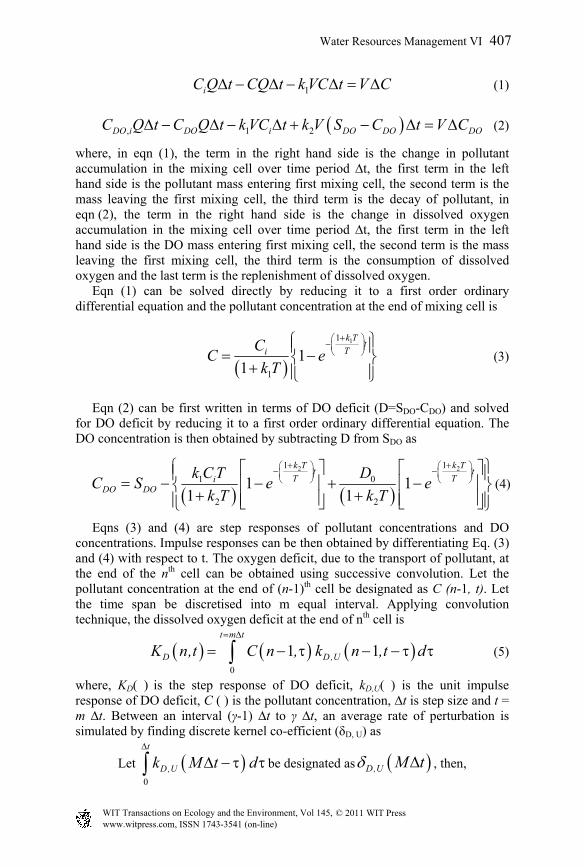
where, in eqn (1), the term in the right hand side is the change in pollutant accumulation in the mixing cell over time period ∆t, the first term in the left hand side is the pollutant mass entering first mixing cell, the second term is the mass leaving the first mixing cell, the third term is the decay of pollutant, in eqn (2), the term in the right hand side is the change in dissolved oxygen accumulation in the mixing cell over time period ∆t, the first term in the left hand side is the DO mass entering first mixing cell, the second term is the mass leaving the first mixing cell, the third term is the consumption of dissolved oxygen and the last term is the replenishment of dissolved oxygen. Eqn (1) can be solved directly by reducing it to a first order ordinary differential equation and the pollutant concentration at the end of mixing cell is

11

1

11

k Tt

TiCC e

k T

(3)

Eqn (2) can be first written in terms of DO deficit (D=SDO-CDO) and solved for DO deficit by reducing it to a first order ordinary differential equation. The DO concentration is then obtained by subtracting D from SDO as

2 21 1

1 0

2 2

1 11 1

k T k Tt t

T TiDO DO

k C T DC S e e

k T k T

(4)

Eqns (3) and (4) are step responses of pollutant concentrations and DO concentrations. Impulse responses can be then obtained by differentiating Eq. (3) and (4) with respect to t. The oxygen deficit, due to the transport of pollutant, at the end of the nth cell can be obtained using successive convolution. Let the pollutant concentration at the end of (n-1)th cell be designated as C (n-1, t). Let the time span be discretised into m equal interval. Applying convolution technique, the dissolved oxygen deficit at the end of nth cell is

0

1 1t m t

D D,UK n,t C n , k n ,t d

(5)

where, KD( ) is the step response of DO deficit, kD,U( ) is the unit impulse response of DO deficit, C ( ) is the pollutant concentration, ∆t is step size and t = m ∆t. Between an interval (γ-1) ∆t to γ ∆t, an average rate of perturbation is simulated by finding discrete kernel co-efficient (δD, U) as

Let 0

t

D,Uk M t d

be designated as D,U M t , then,



1

1 1m

D D,UK n,m t C n , t m , t , n 2

(6)

At the end of the nth cell unit, the dissolved oxygen concentration is then obtained by: CDO (n, m ∆t) = SDO - KD (n, m ∆t) (7)

3 Application to Natural River

The quantity of pollutants entering streams in South African’s rivers has increased tremendously and as result degrading the quality of water downstream. Water quality models are therefore necessary to as they will aid governments in controlling and monitoring stream quality. The study focuses on Baynespruit River situated in Pietermaritzburg, South Africa show in fig. 2. The Baynespruit is a stream passing through the city of Pietermaritzburg in KwaZulu-Natal is devastated by continual solid and liquid waste pollution. The pollution is in the form of sewage discharged from wastewater treatment plants, industrial discharge and household pollution. The river covers a large area and flows through the Pietermaritzburg city’s industrial area before flowing down to a low income area. Due to the poor quality of the water, the residents are no longer able to use the water for domestic, small agricultural and recreational purposes. The flow and other important parameters observed from the stream are presented in table 1.

Table 1: List of parameters obtained on site.

Parameters Values Decay Coefficient k1 (Estimated) 0.0045/s Re-aeration rate k2 (Estimated) 0.0038/s

Width of stream 6.0m Mean stream velocity 0.6m/s

Stream depth 0.25m Dispersion Coefficient, DL

(Estimated) 7.18 m2/s

Stream slope 0.09

4 Simulation of BOD and DO and discussion of results

The water quality data BOD and DO are collected from Baynespruit stream on particular days and tabulated in table 2 and 3 respectively. These tables also show the simulated concentrations of BOD and DO using mixing cells model.



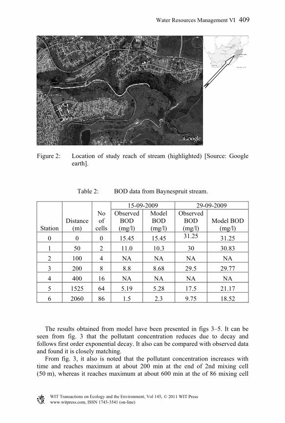
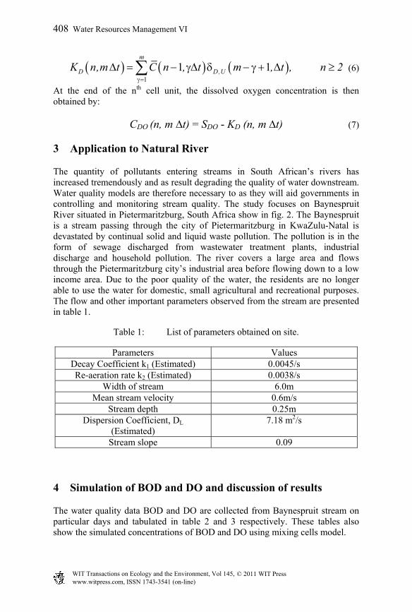
Figure 2: Location of study reach of stream (highlighted) [Source: Google earth].

Table 2: BOD data from Baynespruit stream.

Station Distance

(m)

No of

cells

15-09-2009 29-09-2009 Observed

BOD (mg/l)

Model BOD (mg/l)

Observed BOD (mg/l)

Model BOD (mg/l)

0 0 0 15.45 15.45 31.25 31.25

1 50 2 11.0 10.3 30 30.83

2 100 4 NA NA NA NA

3 200 8 8.8 8.68 29.5 29.77 4 400 16 NA NA NA NA 5 1525 64 5.19 5.28 17.5 21.17 6 2060 86 1.5 2.3 9.75 18.52

The results obtained from model have been presented in figs 3–5. It can be seen from fig. 3 that the pollutant concentration reduces due to decay and follows first order exponential decay. It also can be compared with observed data and found it is closely matching. From fig. 3, it also is noted that the pollutant concentration increases with time and reaches maximum at about 200 min at the end of 2nd mixing cell (50 m), whereas it reaches maximum at about 600 min at the of 86 mixing cell



Table 3: DO data from Baynespruit stream.

Station Distance

(m) No of cells

15-09-2009 Observed DO

(mg/l) Model DO

(mg/l)

0 0 0 9 9.1

1 50 2 0.05 0.00

2 100 4 0.0 0.00

3 200 8 0.0 0.0265 4 400 16 3.1 2.578

5 1525 64 3.7 3.57054 6 2060 86 4.5 4.412027

Figure 3: Variation of BOD concentration with time.

(2060m). Fig 4 shows the variation of DO with time. From fig. 4, the DO concentration of zero denotes that completely polluted river reach. It also can be noted that due to the re-aeration process the DO concentration gets improved at about 2000m (above 80 cells). These characteristics of deoxygenation and re-aeration processes have been confirmed by plotting the DO sag curve and are presented in fig 5. From the fig. 5, one can come to a conclusion that the first 1 km of the river reach is completely polluted.

50m

200m

1525m

2060m



Figure 4: Variation of DO concentration with time.

Figure 5: Variation of DO concentration with space.

5 Conclusion

From the study of the simulation of the temporal and spatial variations of dissolved oxygen in a stream, the following conclusions have been drawn: The mixing cells model in steady state relationship does provide an easier

approach to the evaluation of water quality status of the stream having available data such as velocity, dispersion coefficient and this assumption is widely used and proved to be a valid assumption in this study.

50m 100m

200m

400m 1525m 2060m



Sunrise Settings Ltd

Line

The concentration-time and DO profiles that are produced from the model adequately represent step responses and had agreement with observed data.

The knowledge base and logical deductions that have to be made requires a clear knowledge of the study area and sufficient data collection points around any confluence points such an intersection points of tributaries.

Flexibility of the model is shown to be an advantage when it is required to add other parameters or reaction kinetics. Because the mixing cells model uses first order ODE and adding addition component to the equation will not be a difficult task to solve.

A working Dissolved Oxygen model that has the capability of predicting the temporal and spatial variations of the concentrations have been demonstrated.

From these conclusions, method and results the following recommendations have been advised if further research within this field of dissolved oxygen models is undertaken: By acquiring accurate readings of BOD, COD, cross-sectional area at data

stations relative to the cell size, accurate model comparisons can be made to the model. For the further study to improve the accuracy of results with regard to the cross-sectional area, HEC-RAS may be a useful tool to analyse the steady state water surface profiles at any interval provided that the given information is sufficiently supplied.

By running the model, it is evident that the pollutant concentration as well as the dissolved oxygen concentration can be predicted. With this knowledge, treatment options can be developed under minimal costs compared to continual testing along the reach of the river.

Acknowledgements

Author wants to acknowledge the work done for the collection of data by Mr. Baragarurika, Mr. C. Nair, Mr Zambezi & Mr D Pillai, students, School of Civil Engineering Surveying and Construction, University of KwaZulu-Natal, Durban, South Africa.

References

[1] Banks, R.B., A mixing cell model for longitudinal dispersion in open channels. Water Resources Research, 10(2), pp. 357-358, 1974.

[2] Barnwell, T. O, Rates, Constants and Kinetics Formulations in Surface Water Quality Modeling 2e. Environmental Research Laboratory, U.S. E. P. A, 1985.

[3] Beck, M.B. & Young, P.C., Systematic identification of DO-BOD model structure. Proc A.S.C.E, J. Env. Eng. Div, 102(EE5), pp. 909-927, 1976.



[4] Beer, T., and Young, P. C., Longitudinal Dispersion in Natural Streams. J. Environ. Eng. Div., Am. Soc. Civ. Eng., 109(5), pp. 1049-1067,1983.

[5] Beven, K.J. & Young, P.C., An aggregated mixing zone model of solute transport through porous media. Journal of Contaminant Hydrology, 3(2-4), pp. 129-143, 1988.

[6] Bhargava, D. S., Most rapid BOD assimilation in Ganga and Yamuna rivers. Jour. Env. Engg., ASCE, 109(1), 174-188, 1983.

[7] Bobba, G., V. P. Singh, and L. Bengtsson., Application of first order and Monte Carlo analysis in watershed water quality models. Wat. Resour. Management, 10, 219-240, 1996.

[8] Choudhary, N., P. Tyagi, N. Niyogi, and V. P. Thergonhar., BOD test for tropical countries. ASCE, Jour. of Env. Engineering, 118, 298-303, 1990.

[9] Costa, V.A.F. & Figueiredo, A.R.A., The mixing cells model applied to a fixed bed dryer. The Canadian Journal of Chemical Engineering, 68(5), pp. 876-880, 1990.

[10] Cox B., A review of dissolved oxygen modelling techniques for lowland rivers. The Science of the total environment, 314-316:303-334, 2003.

[11] Davis, P.M. & Atkinson, T.C., Longitudinal dispersion in natural channels: 3. An aggregated dead zone model applied to the River Severn. Hydrol Earth Syst SC, 4(3), pp. 373-381, 2000.

[12] Di Toro, D.M. & O'Connor, D.J., The distribution of dissolved oxygen in a stream with time varying velocity. Water Resources Research, 4(3), pp. 639-646, 1968.

[13] Dobbins, W.E., BOD and oxygen relationship in streams. Proc A.S.C.E, J. Saint. Eng. Div, 90 (SA3), pp. 53-78, 1964.

[14] Dresnack, R. & Dobbins, W.E., Numerical analysis of BOD and DO profiles. Proc A.S.C.E, J. Saint. Eng. Div, 94(SA5), pp. 789-807, 1968.

[15] Hansen, W.D, Frankel, R.J, Economic evaluation of water quality- a mathematical model of dissolved-oxygen concentration in freshwater streams, SERL- Sanitary Engineering Research Laboratory, 1965.

[16] Hassan, N., Longitudinal Dispersion of pollutants in Natural Streams- The Aggregated Dead-Zone Approach, Pertanika J. Sci. & Technol., 1(2), pp. 225-238, 1993.

[17] James, A., (ed) Mathematical Models in Water Pollution Control, 2nd edn, John Wiley and Sons, Newcastle upon Tyne, 1978.

[18] Jolanki, D. G., Basic river water quality models- computer aided learning (CAL) programme on water quality modeling, IHP-V, Technical documents in hydrology, No.13, UNESCO, Paris, 1997.

[19] Katsev, S., Modelling dissolved oxygen dynamics and hypoxia. Biogeoresources, 7(1), pp. 933-957, 2010.

[20] Martin, J.L. & McCutcheon, S.C., Hydrodynamics and transport for water quality modeling, Lewis, Boca Raton, 1998.

[21] O'Connor, D.J., The temporal and spatial distribution of dissolved oxygen in streams. Water Resources Research, 3(1), pp. 65-79, 1967.

[22] Rao, B. K. and D. L. Hathaway, A Three Dimensional Mixing Cell Solute Transport Model and its Application. Ground Water, 27(4), 509–516, 1989.



[23] Rinaldi, Soncini-Sessa, Stehfest and Tamura., Modeling and control of river quality, McGraw hill series in Water Res. And Environ. Engg. Pp. 380, 1979.

[24] Shanahan, P. and D. R. F. Harleman, Transport in Lake Water Quality Modeling. Journal of Environmental Engineering, 110(1), pp. 42–57, 1984.

[25] Smith, P., K. Beven, J. Tawn, S. Blazkova, and L. Merta, Discharge dependent pollutant dispersion in rivers: Estimation of aggregated dead zone parameters with surrogate data. Water Resource Research., 42, W04412, 1984.

[26] Streeter, H. W., and Phelps, E. B., A study of the pollution and natural purification of the Ohio River, Public Health Bulletin No. 146. Public Health Service, Washington, D. C, 1925.

[27] Thomann, R. V., and Mueller, J. A. Principles of surface water quality modelling and control. Harper & Row Publishers, New York, 1987.

[28] Tjomsland, T. Longitudinal Dispersion in a stream Calculated by one dimensional Numerical Model. Nordic Hydrology., 14(1), pp. 41-46, 1983.

[29] Whicker, F. W. and V. Schultz., Radioecology: Nuclear Energy and the Environment, CRC Press, Boca Raton, Florida, 1982.

[30] Young, P. C., Beck, B., The modelling and control of water quality in a river system. Automatica, 10(5), pp. 455-468, 1974



Documents

Simulation of spatial and temporal variations of dissolved oxygen …€¦ · Simulation of spatial and temporal variations of dissolved oxygen of Baynespruit stream in South Africa