365

2008,20(3):365-372

SIMULATION OF SOLUTE TRANSPORT IN A PARALLEL SINGLE FRACTURE WITH LBM/MMP MIXED METHOD*

TAN Ye-fei , ZHOU Zhi-fang College of Civil Engineering, Hohai University, NanJing 210098, China, E-mail: tan8112@hhu.edu.cn

(Received July 30, 2007, Revised October 25, 2007)

Abstract: This article deals with the solute transport in a single fracture with the combination of the Lattice Boltzmann Method (LBM) and Modified Moment Propagation (MMP) method, and this mixed method is proved to have several advantages over the LBM and Moment Propagation (MP) mixed method which leads to negative concentrations under some conditions in computation. The disadvantage of LBM/MP has been overcome to a certain extent. Also, this work presents an LBM solution of modeling single fractures with uniformly or randomly distributed grains, which can provide a new path of applying the LBM in solute transport simulation in fractures.

Key words: Lattice Boltzmann Method (LBM), Modified Moment Propagation (MMP) method, LBM/MMP mixed method, single fracture, solute transport, rough fracture

1. IntroductionWater is the basic source of life and an important

indicator of the quality of our environment. However, the quality and availability of water are increasingly endangered. With the extension of human activities into the underground space, researches on groundwater in fractal rocks and correlative problems become more and more important. Solute transport is one of the problems that have been emphasized by all correlative researchers. However, solute transport is a very complex process, and the fractal rocks are also complex, which make the researches very difficult. The studies on transport have been developed for the storage of nuclear wastes with the development of nuclear industry. In recent years, groundwater in fractal rocks has been threatened by pollutions like storage of nuclear wastes, effusion of contaminated waters caused by wastes burying, incursions of the sea water, leakage of aged oil tubes and so on. For these reasons, many scholars are researching on the characteristics of solute transport in fractal medias [1-3].

* Project supported by the National Natural Science Foundation of China (Grant No. 50579012). Biography: TAN Ye-fei (1981-), Male, Ph. D. Student

Not only physical experimentations have been conducted, but also lots of numerical modeling, and the numerical methods have boomed with the development of computer technology [4-8].

In recent years, the Lattice Boltzmann method (LBM) has won broad recognitions, and this method is an extention of the Lattice Gas Automata (LGA). The particle distributions are denoted by Boolean variables in the LGA model, which may cause heavy noises. The LBM overcame the bugs of the LGA [9], and solved the problem of noises which has harassed the LGA for a long time. This new method has been developed quickly since it was used as a new kind of numerical method for solving partial differential equations, especially in solving the Navier-Stokes equations governing fluid flows [10-16]. The LBM has been applied to many research fields, such as porous media, immiscible liquids, magnetic fluid, reaction-diffusion equation and so on. Traditional modeling methods of Convective Dispersion Equation(CDE) such as the finite difference method and finite volume method are top-down approaches that solve the macroscopic transport equations of mass, momentum, and energy by directly discretizing them. The LBM, on the other hand, is a bottom-up approach that uses kinetic equation models and corresponding relations between the actually simulated statistical

366

dynamics at a microscopic level and transport equations at the macroscopic level [17]. Since the LBM can dispose complex boundaries of flow field, and is adapt to parallel computations, applying the LBM to simulate complex groundwater flows and solute transport has an optimistic foreground.

The Moment Propagation (MP) method was originally developed to efficiently calculate the velocity autocorrelation function in lattice gas cellular automata, later applied to the LBM, and further developed to solve electro-viscous transport problems [18]. Merks et al.[19] presented the Modified Moment Propagation (MMP) method, and it was used to calculate solute transport in tubes combined with the D3Q19 model in the LBM. Since the moment propagation method uses only a single scalar per site for each tracer species, the computational memory requirements are much lower than those for the other methods.

However, there seems no report on applying the LBM to solute transport in fractures. This article combines the D2Q9 model of the LBM with the MMP to simulate the solute transport in a single fracture for the first time. Ideal smooth fracture, fractures with uniformly and randomly distributed grains are all considered. The comparison between the LBM/MP and LBM/MMP shows that the latter educes better results.

2. Lattice Boltzmann Method (LBM) The Boltamann equation can be written as

+ = (f f )ft x

The so called BGK approximation is to assume ( )f as [10]:

(0)1( ) = [ ]f f f

in which f is the lattice distriution function, (0)f is the equilibrium distribution function, and is the relaxation time. If the outside forces are neglected, and discretize the Boltamann equation in temporal and spatial scales, we can obtain

( + , + ) ( , ) =i i if x c t t t f x t

(0)( , ) ( , )i if x t f x t t (1)

This is the so-called LBM-BGK model, in which 0.5 in order to meet the demand of stability, and

is the velocity of particle i . The distribution function

ic( , )if x t can be used to denote the appearing

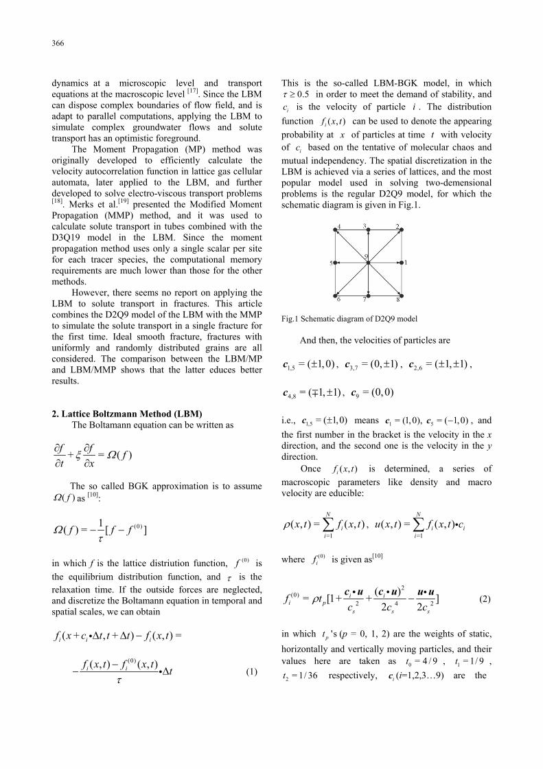
probability at x of particles at time with velocity of based on the tentative of molecular chaos and mutual independency. The spatial discretization in the LBM is achieved via a series of lattices, and the most popular model used in solving two-demensional problems is the regular D2Q9 model, for which the schematic diagram is given in Fig.1.

tic

Fig.1 Schematic diagram of D2Q9 model

And then, the velocities of particles are

1,5 = ( 1,0)c , 3,7 = (0, 1)c , ,2,6 = ( 1, 1)c

4,8 = ( 1, 1)c , 9 = (0,0)c

i.e., means c c , and the first number in the bracket is the velocity in the xdirection, and the second one is the velocity in the ydirection.

1,5 = ( 1,0)c 1 5= (1,0), = ( 1,0)

Once ( , )if x t is determined, a series of macroscopic parameters like density and macro velocity are educible:

=1

( , ) = ( , )N

ii

x t f x t=1

( , ) = ( , )N

i ii

u x t f x t c

i

,

where )(0f is given as[10]

2(0)

2 4

( )= [1+ +2 2

i ii p

s s

f tc c cc u c u u u

2 ]s

(2)

in which (p = 0, 1, 2) are the weights of static, horizontally and vertically moving particles, and their values here are taken as t , ,

respectively, (i=1,2,3…9) are the

'spt

0 = 4 / 9 1 = 1/ 9t

2 = 1/ 36t ic

367

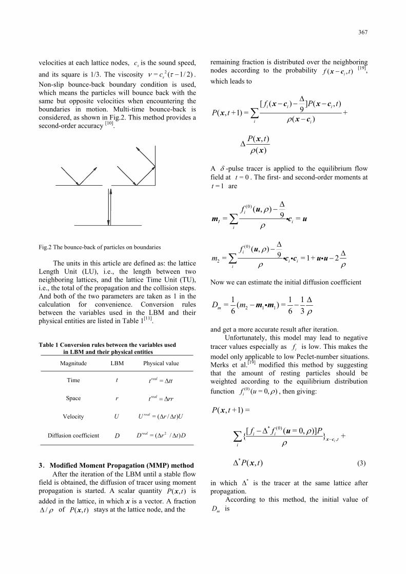
velocities at each lattice nodes, sc is the sound speed, and its square is 1/3. The viscosity .Non-slip bounce-back boundary condition is used, which means the particles will bounce back with the same but opposite velocities when encountering the boundaries in motion. Multi-time bounce-back is considered, as shown in Fig.2. This method provides a second-order accuracy

2= ( 1/ 2)sc

[10].

Fig.2 The bounce-back of particles on boundaries

The units in this article are defined as: the lattice Length Unit (LU), i.e., the length between two neighboring lattices, and the lattice Time Unit (TU), i.e., the total of the propagation and the collision steps. And both of the two parameters are taken as 1 in the calculation for convenience. Conversion rules between the variables used in the LBM and their physical entities are listed in Table 1[11].

Table 1 Conversion rules between the variables used in LBM and their physical entities

Magnitude LBM Physical value

Time t =realt tt

Space r realt rr

UVelocity U = ( / )realU r t

Diffusion coefficient D 2= ( / )realD r t D

3 Modified Moment Propagation (MMP) method After the iteration of the LBM until a stable flow

field is obtained, the diffusion of tracer using moment propagation is started. A scalar quantity ( , )P tx is added in the lattice, in which x is a vector. A fraction

/ of ( , )P tx stays at the lattice node, and the

remaining fraction is distributed over the neighboring nodes according to the probability ( ,i )f tx c [19],which leads to

[ ( ) ] ( , )9( , +1) = +

( )

i i i

i i

f P tP t

x c x cx

x c

( , )( )

P txx

A -pulse tracer is applied to the equilibrium flow field at . The first- and second-order moments at

are = 0t

= 1t

(0) ( , )9= =

i

ii

f um c u

(0)

2

( , )9= = 1+

i

i ii

fm 2

uc c u u

Now we can estimate the initial diffusion coefficient

2 1 11 1= ( ) =6 6mD m 1

3m m

and get a more accurate result after iteration. Unfortunately, this model may lead to negative

tracer values especially as if is low. This makes the model only applicable to low Peclet-number situations. Merks et al.[19] modified this method by suggesting that the amount of resting particles should be weighted according to the equilibrium distribution function (0) ( = 0, )if u , then giving:

( , +1) =P tx

* (0)

,[ ( = 0, )]{ }

i

i it

i

f f Px c

u +

(3) * ( , )P tx

in which * is the tracer at the same lattice after propagation.

According to this method, the initial value of mD is

368

*1 1=6 6mD (4) (4)

Merks et al.[19] suggested that Merks et al.

[19] suggested that

*max

( , )= min[ ]( = 0, )

eqi

eqi

ff

uu

to ensure a sound result. Because the scalar P represents the solute concentration, the solute transport can be modeled by using the MP method [18].It should be noted that this modification can not avoid the illogical negative concentrations absolutely, but to extend the application range, especially removing the limitation on the maximum Peclet number[19].

4 Single fracture models 4.1 Diffusion coefficient

Aris et al. [20] showed that the diffusion coefficient LD between two smooth parallel plates with an aperture of is the result of the integration of molecule diffusion and water flow. And they obey the following linear relation:

b

2 22

Taylor= + = +210L m m

m

U bD D D UD

(5)

where is the average velocity in the fracture. UIn general, the diffusion coefficient in a rough

fracture is larger than that in a smooth one under the same conditions, and increases with the roughness. It can reach 10 times larger than that in a smooth fracture, because the flow field is changed by the grains in a rough fracture. However, the relation between LD and mD would not be constitutionally changed, no matter whether the fracture is rough or not and how rough it is, because LD and still obey the linear relation

2U[21]. So Eq.(5) is still

applicable to rough fractures, and it just needs some adjustments in the aperture. It can be written as follows without considering absorption[22,23]:

22= +

210L mm

UD D bD r

x

(6)

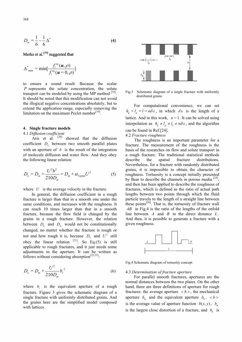
where is the equivalent aperture of a rough fracture. Figure 3 gives the schematic diagram of a single fracture with uniformly distributed grains. And the grains here are the simplified model composed with lattices.

rb

Fig.3 Schematic diagram of a single fracture with uniformly distributed grains

For computational convenience, we can set = = =g gh l l n , in which x is the length of a

lattice. And in this work, . It can be solved using interpolation as

= 1ng g bh l l n x , and the algorithm

can be found in Ref.[24]. 4.2 Fracture roughness

The roughness is an important parameter for a fracture. The measurement of the roughness is the basis of the researches on flow and solute transport in a rough fracture. The traditional statistical methods describe the spatial fracture distributions. Nevertheless, for a fracture with randomly distributed grains, it is impossible to obtain the character of roughness. Tortuosity is a concept initially presented by Bear to describe the channels in porous media [25],and then has been applied to describe the roughness of fractures, which is defined as the ratio of actual path lengths between two points through which the fluid particle travels to the length of a straight line between these points[26]. That is, the tortuosity of fracture wall AB in Fig.4 is the ratio of the lengths of the enfold

line between A and to the direct distance L .And then, it is possible to generate a fracture with a given roughness.

B

Fig.4 Schematic diagram of toruosity concept

4.3 Determination of fracture aperture For parallel smooth fractures, apertures are the

normal distances between the two plates. On the other hand, there are three definitions of aperture for rough fractures: the average aperture , the mechanical aperture and the equivalent aperture .

bmb hb b

is the average value of aperture function ,is the largest close distortion of a fracture, and is

( , )b x y mb

hb

369

a concept brought for the application of cubic law to actual fractures[27].

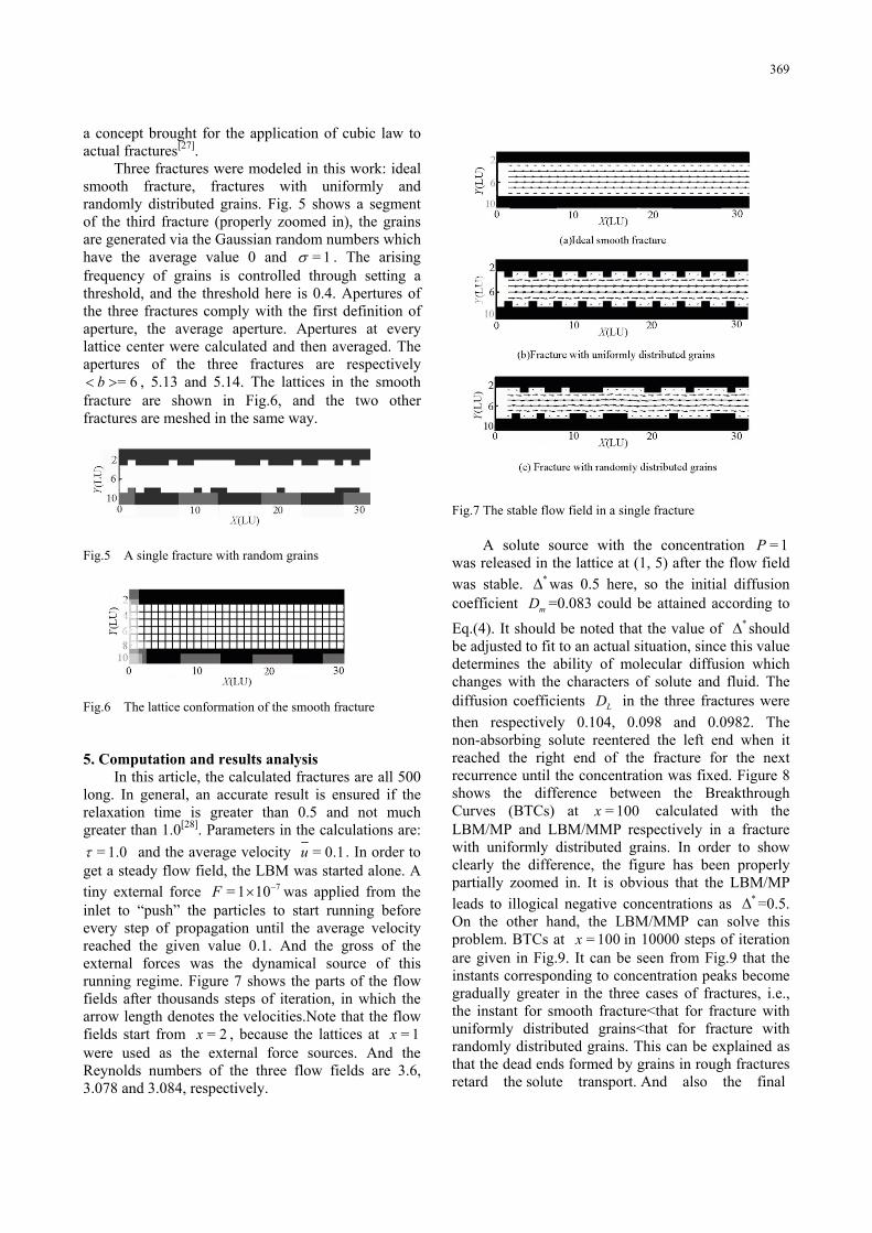
Three fractures were modeled in this work: ideal smooth fracture, fractures with uniformly and randomly distributed grains. Fig. 5 shows a segment of the third fracture (properly zoomed in), the grains are generated via the Gaussian random numbers which have the average value 0 and = 1 . The arising frequency of grains is controlled through setting a threshold, and the threshold here is 0.4. Apertures of the three fractures comply with the first definition of aperture, the average aperture. Apertures at every lattice center were calculated and then averaged. The apertures of the three fractures are respectively

, 5.13 and 5.14. The lattices in the smooth fracture are shown in Fig.6, and the two other fractures are meshed in the same way.

= 6b

Fig.5 A single fracture with random grains

Fig.6 The lattice conformation of the smooth fracture

5. Computation and results analysis In this article, the calculated fractures are all 500

long. In general, an accurate result is ensured if the relaxation time is greater than 0.5 and not much greater than 1.0[28]. Parameters in the calculations are:

= 1.0 and the average velocity = 0.1u . In order to get a steady flow field, the LBM was started alone. A tiny external force was applied from the inlet to “push” the particles to start running before every step of propagation until the average velocity reached the given value 0.1. And the gross of the external forces was the dynamical source of this running regime. Figure 7 shows the parts of the flow fields after thousands steps of iteration, in which the arrow length denotes the velocities.Note that the flow fields start from , because the lattices at

7= 1 10F

= 2x = 1xwere used as the external force sources. And the Reynolds numbers of the three flow fields are 3.6, 3.078 and 3.084, respectively.

Fig.7 The stable flow field in a single fracture

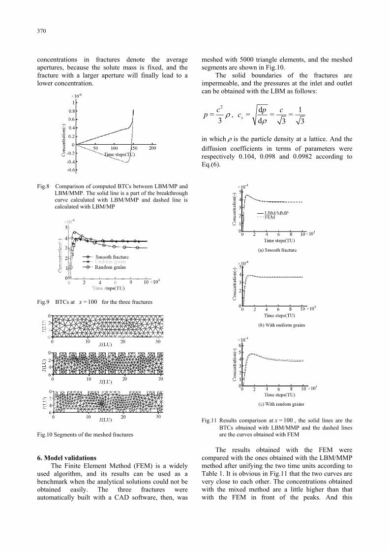
A solute source with the concentration = 1Pwas released in the lattice at (1, 5) after the flow field was stable. * was 0.5 here, so the initial diffusion coefficient mD =0.083 could be attained according to Eq.(4). It should be noted that the value of * should be adjusted to fit to an actual situation, since this value determines the ability of molecular diffusion which changes with the characters of solute and fluid. The diffusion coefficients LD in the three fractures were then respectively 0.104, 0.098 and 0.0982. The non-absorbing solute reentered the left end when it reached the right end of the fracture for the next recurrence until the concentration was fixed. Figure 8 shows the difference between the Breakthrough Curves (BTCs) at calculated with the LBM/MP and LBM/MMP respectively in a fracture with uniformly distributed grains. In order to show clearly the difference, the figure has been properly partially zoomed in. It is obvious that the LBM/MP leads to illogical negative concentrations as

= 100x

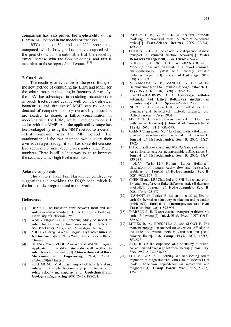
* =0.5. On the other hand, the LBM/MMP can solve this problem. BTCs at in 10000 steps of iteration are given in Fig.9. It can be seen from Fig.9 that the instants corresponding to concentration peaks become gradually greater in the three cases of fractures, i.e., the instant for smooth fracture<that for fracture with uniformly distributed grains<that for fracture with randomly distributed grains. This can be explained as that the dead ends formed by grains in rough fractures retard the solute transport. And also the final

= 100x

370

concentrations in fractures denote the average apertures, because the solute mass is fixed, and the fracture with a larger aperture will finally lead to a lower concentration.

Fig.8 Comparison of computed BTCs between LBM/MP and LBM/MMP. The solid line is a part of the breakthrough curve calculated with LBM/MMP and dashed line is calculated with LBM/MP

Fig.9 BTCs at for the three fractures = 100x

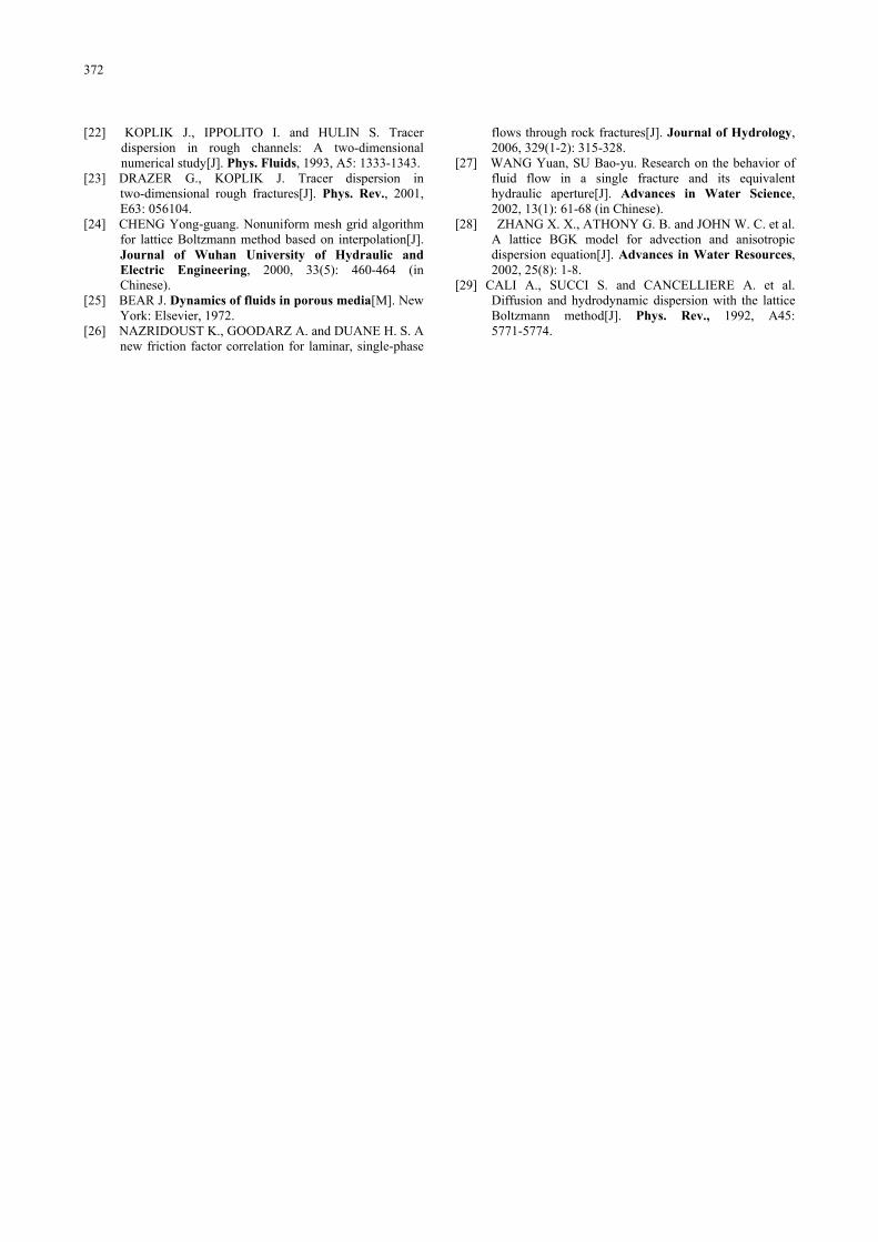
Fig.10 Segments of the meshed fractures

6. Model validationsThe Finite Element Method (FEM) is a widely

used algorithm, and its results can be used as a benchmark when the analytical solutions could not be obtained easily. The three fractures were automatically built with a CAD software, then, was

meshed with 5000 triangle elements, and the meshed segments are shown in Fig.10.

The solid boundaries of the fractures are impermeable, and the pressures at the inlet and outlet can be obtained with the LBM as follows:

2

=3cp ,

d 1= = =d 3 3s

p cc

in which is the particle density at a lattice. And the diffusion coefficients in terms of parameters were respectively 0.104, 0.098 and 0.0982 according to Eq.(6).

Fig.11 Results comparison at , the solid lines are the BTCs obtained with LBM/MMP and the dashed lines are the curves obtained with FEM

= 100x

The results obtained with the FEM were compared with the ones obtained with the LBM/MMP method after unifying the two time units according to Table 1. It is obvious in Fig.11 that the two curves are very close to each other. The concentrations obtained with the mixed method are a little higher than that with the FEM in front of the peaks. And this

371

comparison has also proved the applicability of the LBM/MMP method in the models of fractures.

BTCs at and were also computed, which show good accuracy compared with the predictions. It is mentionable that the modeling errors increase with the flow velocities, and this is accordant to those reported in literature

= 50x = 200x

[29].

7. Conclusion The results give evidences to the good fitting of

the new method of combining the LBM and MMP for the solute transport modeling in fractures. Separately, the LBM has advantages in modeling microstructure of rough fractures and dealing with complex physical boundaries, and the use of MMP can reduce the demand of computer memory remarkably. 9 scalars are needed to denote a lattice concentration in modeling with the LBM, while it reduces to only 1 scalar with the MMP. And the applicability range has been enlarged by using the MMP method to a certain extent compared with the MP method. The combination of the two methods would exert their own advantages, though it still has some deficiencies like remarkable simulation errors under high Peclet numbers. There is still a long way to go to improve the accuracy under high Peclet numbers.

AcknowledgementsThe authors thank Iain Haslam for constructive

suggestions and providing the D2Q9 code, which is the basis of the program used in this work.

References

[1] BEAR J. The transition zone between fresh and salt waters in coastal aquifers [D]. Ph. D. Thesis, Berkeley: University of California, 1960.

[2] WANG Jin-guo, ZHOU Zhi-fang. Study on model of solute transport in fractured rock mass[J]. Rock and Soil Mechanics, 2005, 26(2): 270-276(in Chinese).

[3] ZHOU Zhi-fang, WANG Jin-guo. Hydrodynamics in fracture media[M]. China Water Power Press, 2004 (in Chinese).

[4] HUANG Yong, ZHOU Zhi-fang and WANG Jin-guo. Application of modified stochastic walk method to solute transport simulation[J]. Chinese Journal of Rock Mechanics and Engineering, 2004, 23(14): 2326-2330(in Chinese).

[5] SEKHAR M. Modelling transport of linearly sorbing solutes in a single fracture: asymptotic behavior of solute velocity and dispersivity [J]. Geotechnical and Geological Engineering, 2005, 24(1): 183-201.

[6] KERRY T. B., MAYER K. U. Reactive transport modeling in fractured rock: A state-of-the-science review[J]. Earth-Science Reviews, 2005, 72(3-4): 189-227.

[7] LIN B. S., LEE C. H. Percolation and dispersion of mass transport in saturated fracture networks[J]. WaterResources Management, 1998, 12(66): 409-432.

[8] VOGEL T., GERKE H. H. and ZHANG R. et al. Modeling flow and transport in a two-dimensional dual-permeability system with spatially variable hydraulic properties[J]. Journal of Hydrology, 2002, 238(1): 78-89.

[9] MCNAMARA G. R., ZANETTI G. Use of the Boltzmann-equation to simulate lattice-gas automata[J]. Phys. Rev. Lett., 1988, 61(20): 2332-2335.

[10] WOLF-GLADROW D. A. Lattice-gas cellular automata and lattice Boltzmann models: an introduction[M].Berlin: Springer–Verlag, 2000.

[11] SUCCI S. The lattice Boltzmann method for fluid dynamics and beyond[M]. Oxford, England, UK: Oxford University Press, 2001.

[12] MEI R. W. Lattice Boltzmann method for 3-D flows with curved boundary[J]. Journal of Computational Physics, 2000, 161(2): 680-699.

[13] CHENG Yong-guang, SUO Li-sheng. Lattice Boltzmann scheme to simulate two-dimensional fluid transient[J]. Journal of Hydrodynamics, Ser. B, 2003, 15(2): 19-23.

[14] DU Rui, SHI Bao-chang and WANG Guang-chao et al. An implicit scheme for incompressible LBGK model[J]. Journal of Hydrodynamics, Ser. B, 2005, 17(3): 330-337.

[15] DUAN Ya-li, LIU Ru-xun. Lattice Boltzmann simulations of triagular cavity flow and free-surface problems [J]. Journal of Hydrodynamics, Ser. B,2007,19(2): 127-134.

[16] CHEN Sheng, LIU Zhao-hui and SHI Bao-chang et al. External bodyforce in finite difference lattice Boltzmann method[J]. Journal of Hydrodynamics, Ser. B,2005,17(4): 473-477.

[17] NISHANT G. Lattice Boltzmann method applied to variable thermal conductivity conduction and radiation problems[J]. Journal of Thermophysics and Heat Transfer, 2006, 20(4): 895-902.

[18] WARREN P. B. Electroviscous transport problems via lattice-Boltzmann[J]. Int. J. Mod. Phys., 1997, C8(4): 889-898.

[19] MERKS R. A., HOEKSTRA A. and SLOOT P. The moment propagation method for advection–diffusion in the lattice Boltzmann method: Validation and peclet number limits[J]. J. Comp. Phys., 2002, 183(2): 563-576.

[20] ARIS R. On the dispersion of a solute by diffusion, convection and exchange between phases[J]. Proc. Roy. Soc., 1959, A 252: 538-550.

[21] POT V., GENTY A. Sorbing and non-sorbing solute migration in rough fractures with a multi-species LGA model: dispersion dependence on retardation and roughness [J]. Transp. Porous Med., 2005, 59(22): 175-196.

372

[22] KOPLIK J., IPPOLITO I. and HULIN S. Tracer dispersion in rough channels: A two-dimensional numerical study[J]. Phys. Fluids, 1993, A5: 1333-1343.

[23] DRAZER G., KOPLIK J. Tracer dispersion in two-dimensional rough fractures[J]. Phys. Rev., 2001, E63: 056104.

[24] CHENG Yong-guang. Nonuniform mesh grid algorithm for lattice Boltzmann method based on interpolation[J]. Journal of Wuhan University of Hydraulic and Electric Engineering, 2000, 33(5): 460-464 (in Chinese).

[25] BEAR J. Dynamics of fluids in porous media[M]. New York: Elsevier, 1972.

[26] NAZRIDOUST K., GOODARZ A. and DUANE H. S. A new friction factor correlation for laminar, single-phase

flows through rock fractures[J]. Journal of Hydrology,2006, 329(1-2): 315-328.

[27] WANG Yuan, SU Bao-yu. Research on the behavior of fluid flow in a single fracture and its equivalent hydraulic aperture[J]. Advances in Water Science,2002, 13(1): 61-68 (in Chinese).

[28] ZHANG X. X., ATHONY G. B. and JOHN W. C. et al. A lattice BGK model for advection and anisotropic dispersion equation[J]. Advances in Water Resources,2002, 25(8): 1-8.

[29] CALI A., SUCCI S. and CANCELLIERE A. et al. Diffusion and hydrodynamic dispersion with the lattice Boltzmann method[J]. Phys. Rev., 1992, A45: 5771-5774.