1

SIMULATION OF SHOCK WAVES IN THE INTERPLANETARY MEDIUM

S. Poedts1, B. Van der Holst1, I. Chattopadhyay1, D. Banerjee1, T. Van Lier1, and R. Keppens2

1CPA, K.U.Leuven, Celestijnenlaan 200B, 3001 Leuven, Belgium2FOM Inst. for Plasma Physics Rijnhuizen, Nieuwegein, NL

ABSTRACT

The shocks in the solar corona and interplanetary (IP)space caused by fast Coronal Mass Ejections (CMEs)are simulated numerically and their structure and evolu-tion is studied in the framework of magnetohydrodyna-mics (MHD). Due to the presence of three characteris-tic velocities and the anisotropy induced by the magneticfield, CME shocks generated in the lower corona can havea complex structure including secondary shock fronts,over-compressive and compound shocks, etc. The evo-lution of these CME shocks is followed during their pro-pagation through the solar wind and, in particular, thoughthe critical points in the wind. Particular attention is gi-ven to complex IP events involving two CME shocks col-liding to each other, as often observed. The CME shocksare important for ‘space weather’ because they can easilybe observed in radio wavelengths. This makes it possibleto track the position of the CMEs/magnetic clouds and,hence, to follow their propagation through the corona.

Key words: CMEs, MHD shock waves, solar wind, CMEinteraction, numerical simulations.

1. MOTIVATION AND KEY ROLE OF CMESHOCKS

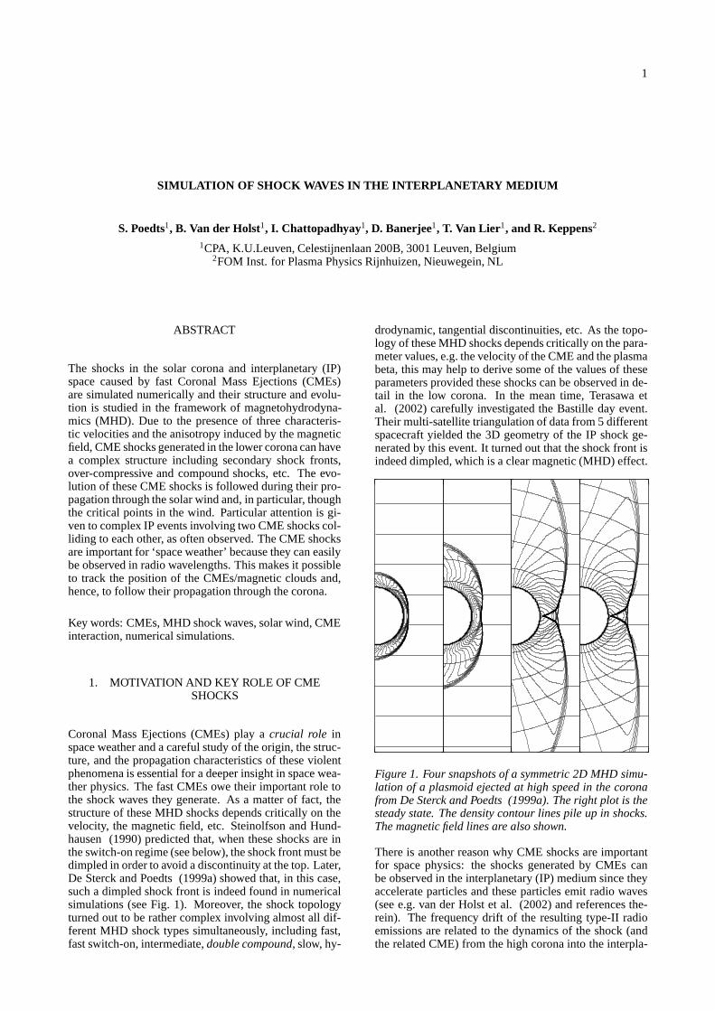
Coronal Mass Ejections (CMEs) play acrucial role inspace weather and a careful study of the origin, the struc-ture, and the propagation characteristics of these violentphenomena is essential for a deeper insight in space wea-ther physics. The fast CMEs owe their important role tothe shock waves they generate. As a matter of fact, thestructure of these MHD shocks depends critically on thevelocity, the magnetic field, etc. Steinolfson and Hund-hausen (1990) predicted that, when these shocks are inthe switch-on regime (see below), the shock front must bedimpled in order to avoid a discontinuity at the top. Later,De Sterck and Poedts (1999a) showed that, in this case,such a dimpled shock front is indeed found in numericalsimulations (see Fig. 1). Moreover, the shock topologyturned out to be rather complex involving almost all dif-ferent MHD shock types simultaneously, including fast,fast switch-on, intermediate,double compound, slow, hy-

drodynamic, tangential discontinuities, etc. As the topo-logy of these MHD shocks depends critically on the para-meter values, e.g. the velocity of the CME and the plasmabeta, this may help to derive some of the values of theseparameters provided these shocks can be observed in de-tail in the low corona. In the mean time, Terasawa etal. (2002) carefully investigated the Bastille day event.Their multi-satellite triangulation of data from 5 differentspacecraft yielded the 3D geometry of the IP shock ge-nerated by this event. It turned out that the shock front isindeed dimpled, which is a clear magnetic (MHD) effect.

Figure 1. Four snapshots of a symmetric 2D MHD simu-lation of a plasmoid ejected at high speed in the coronafrom De Sterck and Poedts (1999a). The right plot is thesteady state. The density contour lines pile up in shocks.The magnetic field lines are also shown.

There is another reason why CME shocks are importantfor space physics: the shocks generated by CMEs canbe observed in the interplanetary (IP) medium since theyaccelerate particles and these particles emit radio waves(see e.g. van der Holst et al. (2002) and references the-rein). The frequency drift of the resulting type-II radioemissions are related to the dynamics of the shock (andthe related CME) from the high corona into the interpla-

2

netary medium. Changes in the shock and CME dyna-mics can be caused by interaction with structures in theinterplanetary space, e.g. collision with another CME,which can lead to shock–dense matter (dense core ofan ejected filament) or shock–shock interaction (Gopals-wamy et al. (2001)).

Clearly, the theoretical modeling of the evolution ofCMEs can be divided into sub-problems. The first sub-problem is the observational study and modeling of thefast and slow ‘quiet’ solar wind. The questions regar-ding, e.g., the heating source(s) and acceleration mecha-nism(s), the required amount of energy, and the locationof the acceleration and heating sources of the fast windcomponent need to be answered. A second sub-problemis the initiation of CMEs. Why do CMEs occur at all andhow are they triggered? Next, there is the sub-problemof the propagation of CMEs and, in particular, the time-height curves need to be understood. Also the evolutionof the structure of the CMEs and the leading shock frontsduring their propagation through the interplanetary me-dium needs to be studied. The modification(s) of theMHD shock structure may contain important clues forunderstanding the propagation properties of CMEs. Theimpact of CMEs or magnetic clouds on the Earth’s ma-gnetosphere is another important sub-problem in whichthe MHD shock complexity is important. The interactionof the CME leading shock front with the bow shock a theEarth’s magnetosphere drastically affects the reconnec-tion characteristics of the magnetic field lines and, hence,certainly influences the ’geo-effectiveness’ of the magne-tic storms. In the present paper, we concentrate on simu-lations of the evolution of CMEs in the IP medium.

As the CME relatedcomplex MHD shocks may play akeyrole in the above-mentioned sub-problems we will firstbriefly discuss the possible components of the complexMHD shocks generated by fast CMEs.

MHD shocks

As is well-known from fluid dynamics, a supersonic flowfinds its way around an object by creating a bow shockin front of it. In a magnetized plasma, the magnetic fieldintroduces a preferred direction and, hence,anisotropy.Moreover, in the MHD description of such a plasma,there existthree basic MHD waves, viz. the Alfven waveand the slow and fast magnetosonic waves, instead ofjust sound waves. The anisotropy of these three wavemodes results in MHD shocks which can be much morecomplex than the shocks in hydrodynamic systems whichhave only one (isotropic) wave speed. The characteristicvelocities of the three MHD waves depend on the direc-tion of propagation and for a direction labeled byx, thesevelocities are denoted bycAx, csx, andcfx, respectively.They always (i.e. for any directionx) satisfy the relationcfx ≥ cAx ≥ csx.

When thex−direction now denotes the direction perpen-dicular to the shock front, this means there are four pos-sible positions for the normal plasma speed,vx, viz.

[1] ≥ cfx ≥ [2] ≥ cAx ≥ [3] ≥ csx ≥ [4],

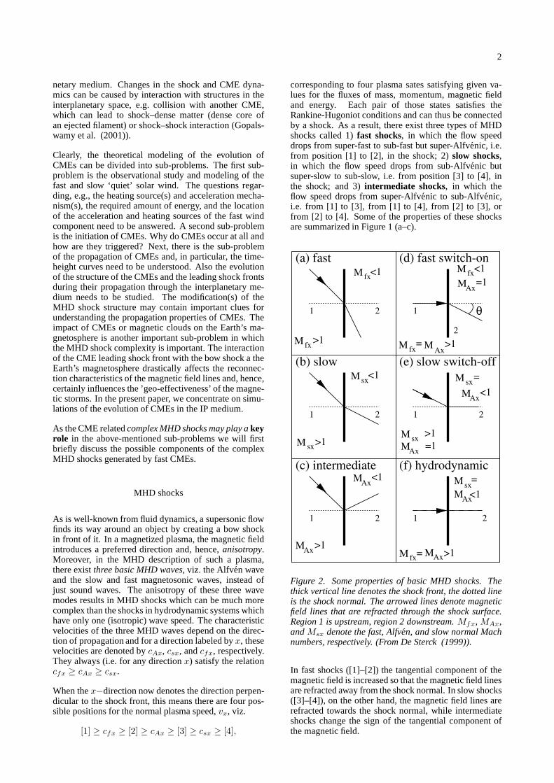
corresponding to four plasma sates satisfying given va-lues for the fluxes of mass, momentum, magnetic fieldand energy. Each pair of those states satisfies theRankine-Hugoniot conditions and can thus be connectedby a shock. As a result, there exist three types of MHDshocks called 1)fast shocks, in which the flow speeddrops from super-fast to sub-fast but super-Alfvenic, i.e.from position [1] to [2], in the shock; 2)slow shocks,in which the flow speed drops from sub-Alfvenic butsuper-slow to sub-slow, i.e. from position [3] to [4], inthe shock; and 3)intermediate shocks, in which theflow speed drops from super-Alfvenic to sub-Alfvenic,i.e. from [1] to [3], from [1] to [4], from [2] to [3], orfrom [2] to [4]. Some of the properties of these shocksare summarized in Figure 1 (a–c).

2

(a) fast (d) fast switch-on

(e) slow switch-off(b) slow

(c) intermediate (f) hydrodynamic

1

1

1

1

12

M

21

>1

2

=1

2

fx

2

M fx

M fx M fx

M fx

MAx

M sx

MAx

M sxM

AxM sx

MAx

MAx

M

<1

M sx<1

Ax

M sx

>1

<1 <1

=1

=

>1

>1

= MAx>1

<1

<1

>1

=

= MAx

θ

Figure 2. Some properties of basic MHD shocks. Thethick vertical line denotes the shock front, the dotted lineis the shock normal. The arrowed lines denote magneticfield lines that are refracted through the shock surface.Region 1 is upstream, region 2 downstream.Mfx, MAx,andMsx denote the fast, Alfven, and slow normal Machnumbers, respectively. (From De Sterck (1999)).

In fast shocks ([1]–[2]) the tangential component of themagnetic field is increased so that the magnetic field linesare refracted away from the shock normal. In slow shocks([3]–[4]), on the other hand, the magnetic field lines arerefracted towards the shock normal, while intermediateshocks change the sign of the tangential component ofthe magnetic field.

3

Each of the MHD shock types has a ‘limiting case’, alsoindicated in Fig. 2. A fast ‘switch-on’ shock, e.g., hasa vanishing tangential component of the magnetic fieldupstream, but a finite one downstream, while in a slow‘switch-off’ this magnetic field component is ‘switchedoff’ by the shock, i.e. it vanishes downstream. A [1]–[4] hydrodynamic shock is a limiting case of an interme-diate shock that does not change the magnetic field (seeFig. 2(f)).

Intermediate shocks and fast switch-on shocks can onlyoccur for some well-specified regime of the upstream pa-rameters. Switch-on shocks are intrinsically magneticphenomena that have no analogue in hydrodynamic flowsof neutral fluids. They can only occur when the upstreammagnetic field,B1 is dominant, i.e.

B2

1> γp1, (1)

and

B2

1 > ρ1v2

x,1

γ − 1

γ(1 − β1) + 1, (2)

where vx,1 is the upstream velocity component alongthe shock normal andp1 and β1 the upstream thermalpressure and plasma beta, respectively; whileγ denotesthe ratio of specific heats. These conditions are derivedfrom the Rankine-Hugoniot jump conditions in 1D MHDflows (Kennel et al. (1989); Steinolfson and Hundhausen(1990)).

2. MODELING THE (PRE-EVENT) SOLAR WIND

Wang et al. (1995) showed with a parameter study thatthe pre-event corona is a crucial factor in dictating CMEproperties. Hence, we will first discuss the modeling ofthe solar wind separately. We focus only on those windsolutions used for CME evolution studies.

2.1. Spherically symmetric (1D) wind models

Historical starting points for solar wind models are theParker (1958) wind, a spherically symmetric (1D), un-magnetized (hydrodynamic) solution; and the Weber &Davis (1967) wind model which constitutes a valuableextension to the rotating, polytropic Parker wind witha radial and toroidal magnetic field component. La-ter, these one-dimensional models were perfected as evermore physical effects were taken into account. As a mat-ter of fact, such geometrically simple models are stillfrequently used to study e.g. magnetic loops in closed-field regions of the solar corona or the outflow in co-ronal holes. They have the advantage that complicated(thermo-)dynamic effects, such as thermal conductivity)can easily included. These 1D models also include atleast part of the transition region and radiative losses.Moreover, they are usually not very CPU-intensive. ForCME evolution, however, their geometric limitations area major disadvantage: open and closed magnetic field re-gions cannot be treated simultaneously in these models.

2.2. Axisymmetric (2D and 2.5d) wind models

Pneuman & Kopp (1971) constructed the first two-dimensional (axisymmetric) MHD model for the solarcorona by solving the steady state equations. This modelincluded both a helmet streamer and open field regions.Sakurai (1985, 1990) derived an analytical 2D generali-zation of the Weber-Davis wind model. Most axisymme-tric wind models, however, are numerical solutions ob-tained by integrating the time-dependent MHD equationsby using a time-asymptotic approach. The energy equa-tion is often simplified, e.g. by considering a polytropicrelation between pressure and density, sometimes evenisothermal. Such simplified polytropic models yield sur-prisingly good approximations and can reproduce manyqualitative features of the observed solar corona. But theplasma density and temperature in these models are notin quantitative agreement with the observations. There-fore, more recent models focus on improving the energyequation. Below, we briefly discuss some of these modelsthat have been used to simulate the evolution of ICMEsand, in particular, the MHD shocks they generate.

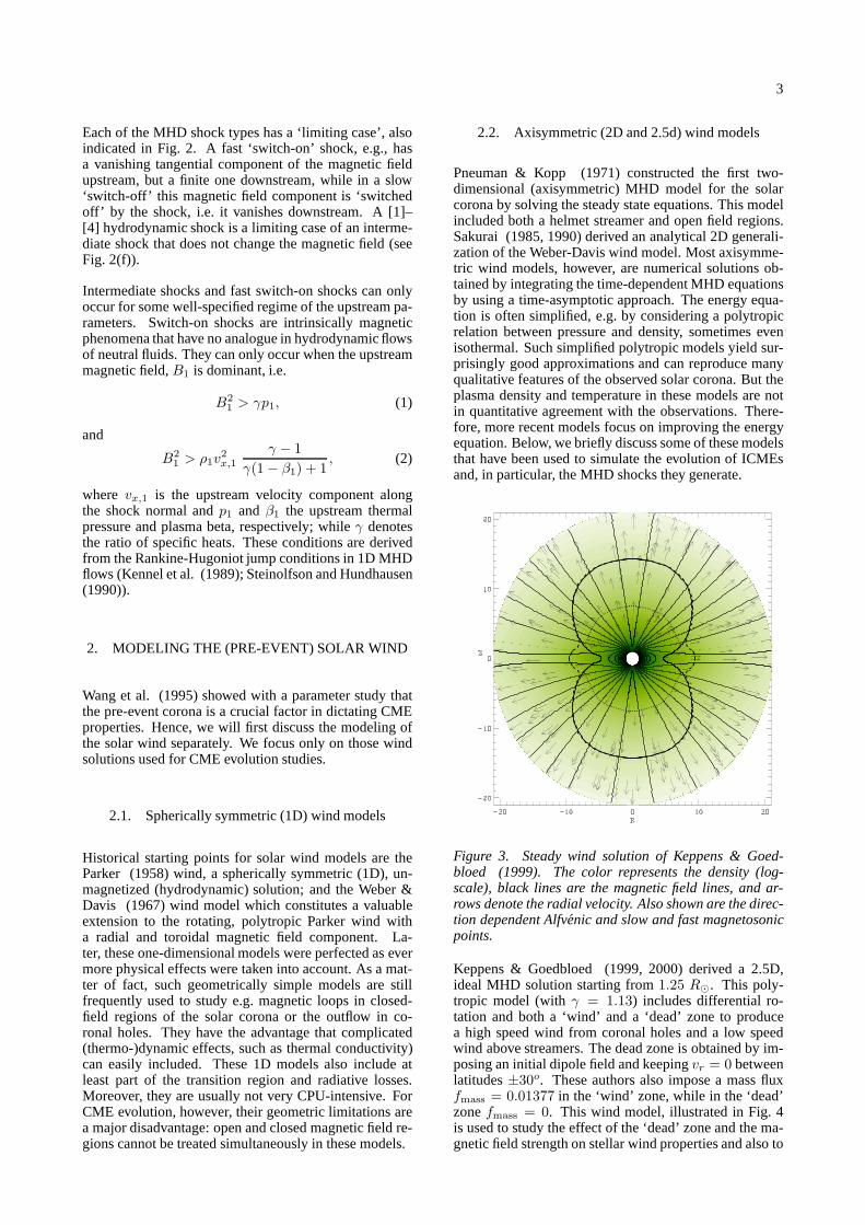
Figure 3. Steady wind solution of Keppens & Goed-bloed (1999). The color represents the density (log-scale), black lines are the magnetic field lines, and ar-rows denote the radial velocity. Also shown are the direc-tion dependent Alfvenic and slow and fast magnetosonicpoints.

Keppens & Goedbloed (1999, 2000) derived a 2.5D,ideal MHD solution starting from1.25 R�. This poly-tropic model (withγ = 1.13) includes differential ro-tation and both a ‘wind’ and a ‘dead’ zone to producea high speed wind from coronal holes and a low speedwind above streamers. The dead zone is obtained by im-posing an initial dipole field and keepingvr = 0 betweenlatitudes±30o. These authors also impose a mass fluxfmass = 0.01377 in the ‘wind’ zone, while in the ‘dead’zonefmass = 0. This wind model, illustrated in Fig. 4is used to study the effect of the ‘dead’ zone and the ma-gnetic field strength on stellar wind properties and also to

4

study CME evolution (see below).

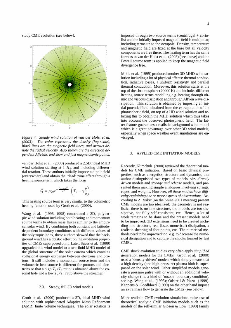
Figure 4. Steady wind solution of van der Holst et al.(2003). The color represents the density (log-scale),black lines are the magnetic field lines, and arrows de-note the radial velocity. Also shown are the direction de-pendent Alfvenic and slow and fast magnetosonic points.

van der Holst et al. (2003) produced a 2.5D, ideal MHDwind solution starting at1 R� and including differen-tial rotation. These authors initially impose a dipole field(everywhere) and obtain the ‘dead’ zone effect through aheating source term which takes the form

Q = ρq0e−

(r−r0)2

σ2

(

T0 − γp

ρ

)

.

This heating source term is very similar to the volumetricheating function used by Groth et al. (2000).

Wang et al. (1995, 1998) constructed a 2D, polytro-pic wind solution including both heating and momentumsource terms to obtain mass fluxes similar to the empiri-cal solar wind. By combining both constant and latitude-dependent boundary conditions with different values ofthe polytropic index, these authors showed that the back-ground wind has a drastic effect on the evolution proper-ties of CMEs superposed on it. Later, Suess et al. (1999)upgraded this wind model to a two-fluid MHD model ofthe global structure of the solar corona which containscollisional energy exchange between electrons and pro-tons. It still includes a momentum source term and thevolumetric heat source is different for protons and elec-trons so that a highTp/Te ratio is obtained above the co-ronal hole and a lowTp/Te ratio above the streamer.

2.3. Steady, full 3D wind models

Groth et al. (2000) produced a 3D, ideal MHD windsolution with sophisticated Adaptive Mesh Refinement(AMR) finite volume techniques. The solar rotation is

imposed through two source terms (centrifugal + corio-lis) and the initially imposed magnetic field is multipolar,including terms up to the octupole. Density, temperatureand magnetic field are fixed at the base but all velocitycomponents are free there. The heating term has the sameform as in van der Holst et al. (2003) (see above) and thePowell source term is applied to keep the magnetic fielddivergence free.

Mikic et al. (1999) produced another 3D MHD wind so-lution including a lot of physical effects: thermal conduc-tion, radiative losses, a uniform resistivity and parallelthermal conduction. Moreover, this solution starts at thetop of the chromosphere (20000 K) and includes differentheating source terms modelling e.g. heating through oh-mic and viscous dissipation and through Alfven wave dis-sipation. This solution is obtained by imposing an ini-tial potential field, obtained from the extrapolation of thephotospheric field, on top of a HD wind solution and re-laxing this to obtain the MHD solution which thus takesinto account the observed photospheric field. The lat-ter feature guarantees a realistic background wind modelwhich is a great advantage over other 3D wind models,especially when space weather event simulations are en-visaged.

3. APPLIED CME INITIATION MODELS

Recently, Klimchuk (2000) reviewed the theoretical mo-dels for CME initiation. Based on basic physical pro-perties, such as energetics, structure and dynamics, thisauthor distinguished two types of models, viz.directlydrivenmodels andstorage and releasemodels, and pre-sented them making simple analogues involving springs,ropes, and weights. However,all these models have diffi-culty explaining one or more aspects of observations.Ac-cording to Z. Mikic (on the Shine 2001 meeting) presentCME models are too idealized: the geometry is not rea-listic, there is no fine structure, the models are too dis-sipative, not fully self-consistent, etc. Hence, a lot ofwork remains to be done and the present models needto be improved: 3D extensions need to be created inclu-ding fine structure, real (i.s.o. numerical) dissipation, arealistic shearing of foot points, etc. The numerical me-thods need to be improved too, e.g. to decrease the nume-rical dissipation and to capture the shocks formed by fastCMEs.

CME shock evolution studies very often applysimplifiedgeneration models for the CMEs. Groth et al. (2000)used a ‘density-driven’ models which simply means thata high-density (and high-pressure) plasma blob is super-posed on the solar wind. Other simplified models gene-rate a pressure pulse with or without an additional velo-city change (i.e. a kind of ‘nozzle’ boundary condition),see e.g. Wang et al. (1995); Odstrcil & Pizzo (1999).Keppens & Goedbloed (1999) on the other hand imposean extra mass flow to generate the CMEs (see below).

More realistic CME evolution simulations make use oftheoretical analytic CME initiation models such as themodels of the self-similar Gibson & Low (1998) family

5

(Gombosi et al. (2000)) or the Titov & Demoulin mo-del (Roussev et al. (2003)). Odstrcil & Pizzo (2002)and Odstrcil et al. (2002) still use another analytical fluxrope model. What one really should do, however, is to si-mulate the evolution of reconstructed coronal structures(e.g. Aulanier et al. (2000)) driven unstable by foot pointshearing and/or flux emergence or cancellation. Severalgroups are working on such simulations and results willappear in the near future.

4. CME PROPAGATION AND CME-CMEINTERACTIONS

The shocks generated by CMEscan be observed in theinterplanetary (IP) medium due to the fact that they ac-celerate particles and these accelerated particles emit ra-dio waves. We know that the IP signals of CMEs do notpossess the typical three-part structure of most CMEs inthe low corona (bright loop, dark void, bright inner ker-nel). However, a lot of key questions remain to be ans-wered, e.g. How do CMEs propagate through the solarwind? At what speeds?; Can the speed of a CME beconstant?; What is the geometrical structure of the as-sociated shocks?; How does the type and geometry of theshocks change at the critical points in the wind?

Evolution of single CMEs

van der Holst et al. (2003) superposed a CME ontheir 2.5D MHD wind solution discussed above (Fig. 4).They used the simplified ‘density(+pressure)-driven’mo-del and simulated CMEs both in the equatorial streamerbelt and at larger latitudes (see Fig. 5).

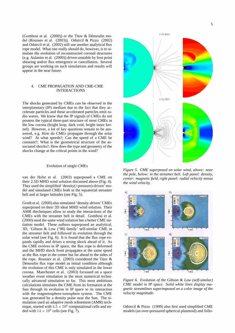
Groth et al. (2000) also simulated ‘density-driven’ CMEssuperposed on their 3D ideal MHD wind solution. TheirAMR thechniques allow to study the interactions of theCMEs with the streamer belt in detail. Gombosi et al.(2000) used the same wind solution but a better CME ini-tiation model. These authors superposed an analytical,3D, ‘Gibson & Low (’98) family’ self-similar CME inthe streamer belt and followed its evolution through thesolar wind (see Fig. 6). It is found that the flux rope ex-pands rapidly and drives a strong shock ahead of it. Asthe CME evolves in IP space, the flux rope is deformedand the MHD shock front propagates at the same speedas the flux rope in the center but far ahead to the sides ofthe rope. Roussev et al. (2003) considered the Titov &Demoulin flux rope model as initial condition althoughthe evolution of this CME is only simulated in the lowercorona. Manchester et al. (2003) focussed on a spaceweather event simulation in the most numerical techni-cally advanced simulation so far. This most ambitiouscalculations simulates the CME from its formation at theSun through its evolution in IP space to its interactionwith the magnetosphere-ionosphere system. The CMEwas generated by a density pulse near the Sun. The si-mulation used an adaptive mesh refinement (AMR) tech-nique, started with4.5× 106 computational cells and en-ded with14 × 106 cells (see Fig. 7).

Figure 5. CME superposed on solar wind, above: nearthe pole, below: in the streamer belt. Left panel: density,center: magnetic field, right panel: radial velocity minusthe wind velocity.

Figure 6. Evolution of the Gibson & Low (self-similar)CME model in IP space. Solid white lines display ma-gnetic streamlines superimposed on a color image of thevelocity magnitude.

Odstrcil & Pizzo (1999) also first used simplified CMEmodels (an over-pressured spherical plasmoid) and follo-

6

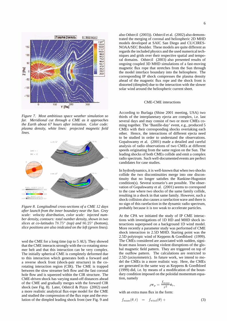
Figure 7. Most ambitious space weather simulation sofar. Meridional cut through a CME as it approachesthe Earth about 67 hours after initiation. Color code:plasma density, white lines: projected magnetic fieldlines.

Figure 8. Longitudinal cross-sections of a CME 12 daysafter launch from the inner boundary near the Sun. Greyscale: velocity distribution, color scale: injected num-ber density, contours: total number density, shown in twoslices at co-latitudes78.75o (top) and86.25o (bottom),slice positions are also inidcated on the left (green lines).

wed the CME for a long time (up to 5 AU). They showedthat the CME interacts strongly with the co-rotating strea-mer belt and that this interaction can be very complex.The initially spherical CME is completely deformed dueto this interaction which generates both a forward anda reverse shock front (shock-pair structure) in the co-rotating interaction region (CIR). The CME is trappedbetween the slow streamer belt flow and the fast coronalhole flow and is squeezed within the CIR structure. TheCME-driven shock has varying stand-off distances aheadof the CME and gradually merges with the forward CIRshock (see Fig. 8). Later, Odstrcil & Pizzo (2002) useda more realistic analytical flux-rope model for the CMEand studied the compression of the flux rope and the evo-lution of the dimpled leading shock front (see Fig. 9 and

also Odstrcil (2003)). Odstrcil et al. (2002) also demons-trated the merging of coronal and heliospheric 2D MHDmodels developed at SAIC San Diego and CU/CIRES-NOAA/SEC Boulder. These models are quite different asregards the included physics and the used numerical tech-niques and grids over their respective spatial and tempo-ral domains. Odstrcil (2003) also presented results ofongoing coupled 3D MHD simulations of a fast-movingmagnetic flux rope that stretches from the Sun throughthe model interface boundary into the heliosphere. Thecorresponding IP shock compresses the plasma densityahead of the magnetic flux rope and the shock front isdistorted (dimpled) due to the interaction with the slowersolar wind around the heliospheric current sheet.

CME-CME interactions

According to Burlaga (Shine 2001 meeting, USA) twothirds of the interplanetary ejecta are complex, i.e. lastseveral days and may consist of two or more CMEs co-ming together. The ‘Bastille-day’ event, e.g., produced 5CMEs with their corresponding shocks overtaking eachother. Hence, the interactions of different ejecta needto be studied in order to understand the observations.Gopalswamy et al. (2001) made a detailed and carefulanalysis of radio observations of two CMEs at differentspeeds originating from the same region on the Sun. Theleading shocks of both CMEs collide and emit a complexradio spectrum. Such well-documented events are perfectcandidates for case studies.

In hydrodynamics, it is well-known that when two shockscollide the two discontinuities merge into one discon-tinuity that no longer satisfies the Rankine-Hugoniotcondition(s). Several scenario’s are possible. The obser-vation of Gopalswamy et al. (2001) seems to correspondto the case where two shocks of the same family collide,resulting in a shock in that same family. However, such ashock collision also causes a rarefaction wave and there isno sign of this rarefaction in the dynamic radio spectrum,probably because it is too weak to accelerate particles.

At the CPA we initiated the study of IP CME interac-tions with investigations of 1D HD and MHD shock in-teractions superposed on a background 1D wind model.More recently a parameter study was performed of CMEshock interaction in 2.5D MHD. Starting point was the2.5D polytropic wind of Keppens & Goedbloed (1999).The CMEs considered are associated with sudden, signi-ficant mass losses causing violent disruptions of the glo-bal magnetic field pattern. They are triggered on top ofthe outflow pattern. The calculations are restricted to2.5D (axisymmetric). In future work, we intend to mo-del the CMEs in a more realistic way. Here, the CMEsare generated in the same way as Keppens & Goedbloed(1999) did, i.e. by means of a modification of the boun-dary condition imposed on the poloidal momentum equa-tion, namely

ρvp =fmass

r2er,

with an extra mass flux in the form:

fmass(θ, t) = fwind(θ) + (3)

7

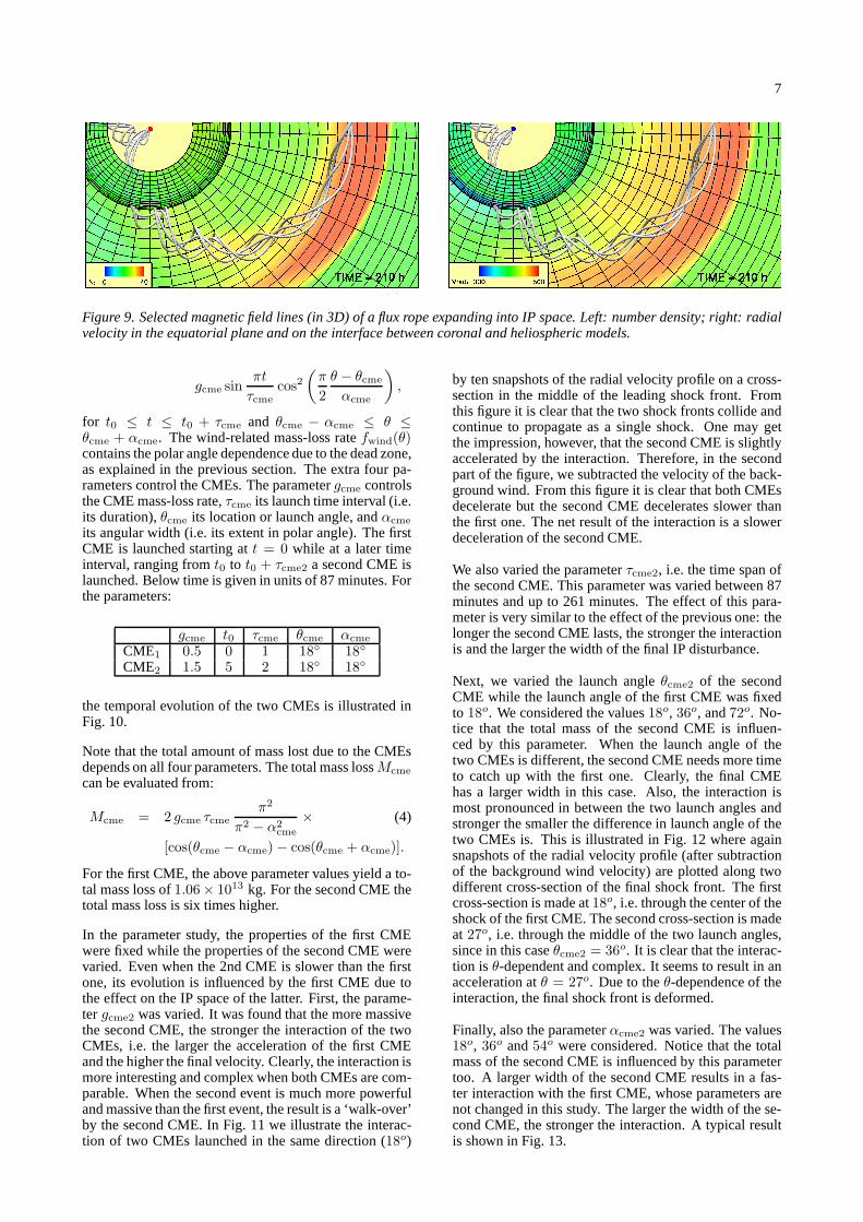
Figure 9. Selected magnetic field lines (in 3D) of a flux rope expanding into IP space. Left: number density; right: radialvelocity in the equatorial plane and on the interface between coronal and heliospheric models.

gcme sinπt

τcme

cos2(

π

2

θ − θcme

αcme

)

,

for t0 ≤ t ≤ t0 + τcme and θcme − αcme ≤ θ ≤

θcme + αcme. The wind-related mass-loss ratefwind(θ)contains the polar angle dependence due to the dead zone,as explained in the previous section. The extra four pa-rameters control the CMEs. The parametergcme controlsthe CME mass-loss rate,τcme its launch time interval (i.e.its duration),θcme its location or launch angle, andαcme

its angular width (i.e. its extent in polar angle). The firstCME is launched starting att = 0 while at a later timeinterval, ranging fromt0 to t0 + τcme2 a second CME islaunched. Below time is given in units of 87 minutes. Forthe parameters:

gcme t0 τcme θcme αcme

CME1 0.5 0 1 18◦ 18◦

CME2 1.5 5 2 18◦ 18◦

the temporal evolution of the two CMEs is illustrated inFig. 10.

Note that the total amount of mass lost due to the CMEsdepends on all four parameters. The total mass lossMcme

can be evaluated from:

Mcme = 2 gcme τcme

π2

π2 − α2cme

× (4)

[cos(θcme − αcme) − cos(θcme + αcme)].

For the first CME, the above parameter values yield a to-tal mass loss of1.06× 1013 kg. For the second CME thetotal mass loss is six times higher.

In the parameter study, the properties of the first CMEwere fixed while the properties of the second CME werevaried. Even when the 2nd CME is slower than the firstone, its evolution is influenced by the first CME due tothe effect on the IP space of the latter. First, the parame-ter gcme2 was varied. It was found that the more massivethe second CME, the stronger the interaction of the twoCMEs, i.e. the larger the acceleration of the first CMEand the higher the final velocity. Clearly, the interaction ismore interesting and complex when both CMEs are com-parable. When the second event is much more powerfuland massive than the first event, the result is a ‘walk-over’by the second CME. In Fig. 11 we illustrate the interac-tion of two CMEs launched in the same direction (18o)

by ten snapshots of the radial velocity profile on a cross-section in the middle of the leading shock front. Fromthis figure it is clear that the two shock fronts collide andcontinue to propagate as a single shock. One may getthe impression, however, that the second CME is slightlyaccelerated by the interaction. Therefore, in the secondpart of the figure, we subtracted the velocity of the back-ground wind. From this figure it is clear that both CMEsdecelerate but the second CME decelerates slower thanthe first one. The net result of the interaction is a slowerdeceleration of the second CME.

We also varied the parameterτcme2, i.e. the time span ofthe second CME. This parameter was varied between 87minutes and up to 261 minutes. The effect of this para-meter is very similar to the effect of the previous one: thelonger the second CME lasts, the stronger the interactionis and the larger the width of the final IP disturbance.

Next, we varied the launch angleθcme2 of the secondCME while the launch angle of the first CME was fixedto 18o. We considered the values18o, 36o, and72o. No-tice that the total mass of the second CME is influen-ced by this parameter. When the launch angle of thetwo CMEs is different, the second CME needs more timeto catch up with the first one. Clearly, the final CMEhas a larger width in this case. Also, the interaction ismost pronounced in between the two launch angles andstronger the smaller the difference in launch angle of thetwo CMEs is. This is illustrated in Fig. 12 where againsnapshots of the radial velocity profile (after subtractionof the background wind velocity) are plotted along twodifferent cross-section of the final shock front. The firstcross-section is made at18o, i.e. through the center of theshock of the first CME. The second cross-section is madeat 27o, i.e. through the middle of the two launch angles,since in this caseθcme2 = 36o. It is clear that the interac-tion is θ-dependent and complex. It seems to result in anacceleration atθ = 27o. Due to theθ-dependence of theinteraction, the final shock front is deformed.

Finally, also the parameterαcme2 was varied. The values18o, 36o and54o were considered. Notice that the totalmass of the second CME is influenced by this parametertoo. A larger width of the second CME results in a fas-ter interaction with the first CME, whose parameters arenot changed in this study. The larger the width of the se-cond CME, the stronger the interaction. A typical resultis shown in Fig. 13.

8

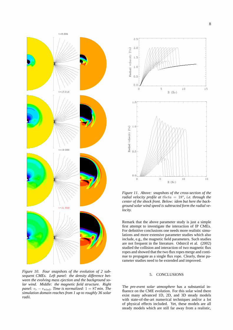
Figure 10. Four snapshots of the evolution of 2 sub-sequent CMEs. Left panel: the density difference bet-ween the evolving mass ejection and the background so-lar wind. Middle: the magnetic field structure. Rightpanel: vr − vwind. Time is normalized:1 = 87 min. Thesimulation domain reaches from 1 up to roughly 36 solarradii.

Figure 11. Above: snapshots of the cross-section of theradial velocity profile attheta = 18o, i.e. through thecenter of the shock front. Below: idem but here the back-ground solar wind speed is subtracted form the radial ve-locity.

Remark that the above parameter study is just a simplefirst attempt to investigate the interaction of IP CMEs.For definitive conclusions one needs more realistic simu-lations and more extensive parameter studies which alsoinclude, e.g., the magnetic field parameters. Such studiesare not frequent in the literature. Odstrcil et al. (2002)studied the collision and interaction of two magnetic fluxropes and showed that the two flux ropes merge and conti-nue to propagate as a single flux rope. Clearly, these pa-rameter studies need to be extended and improved.

5. CONCLUSIONS

The pre-event solar atmospherehas a substantial in-fluence on the CME evolution. For this solar wind thereexist many advanced 1D, 2D, and 3D steady modelswith state-of-the-art numerical techniques and/or a lotof physical effects included. Yet, these models are allsteady models which are still far away from a realistic,

9

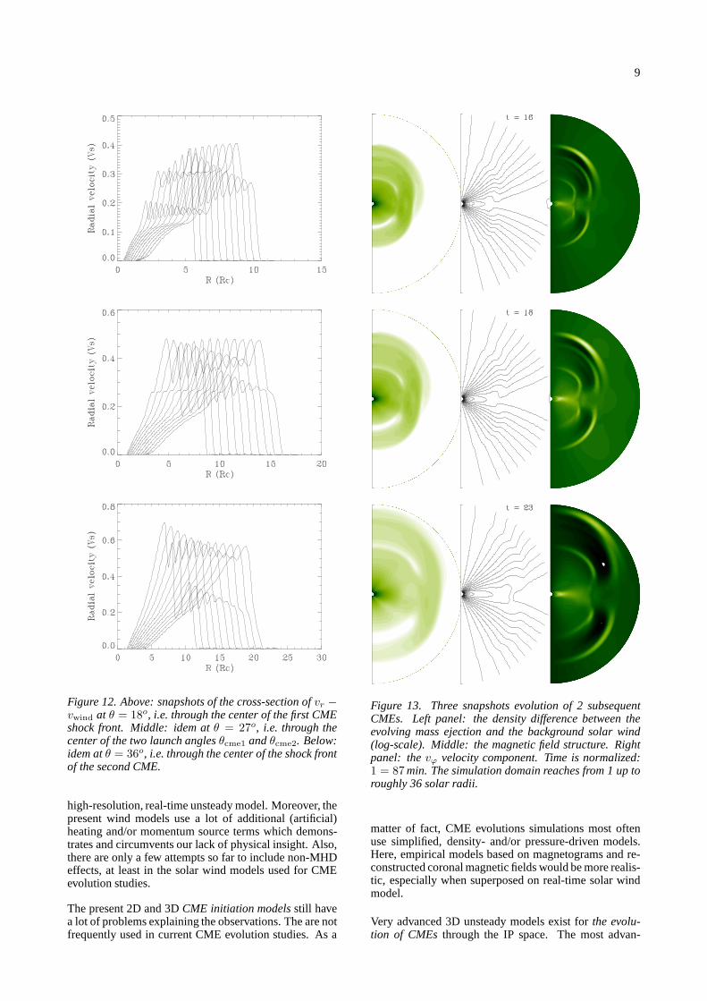
Figure 12. Above: snapshots of the cross-section ofvr −

vwind at θ = 18o, i.e. through the center of the first CMEshock front. Middle: idem atθ = 27o, i.e. through thecenter of the two launch anglesθcme1 andθcme2. Below:idem atθ = 36o, i.e. through the center of the shock frontof the second CME.

high-resolution, real-time unsteady model. Moreover, thepresent wind models use a lot of additional (artificial)heating and/or momentum source terms which demons-trates and circumvents our lack of physical insight. Also,there are only a few attempts so far to include non-MHDeffects, at least in the solar wind models used for CMEevolution studies.

The present 2D and 3DCME initiation modelsstill havea lot of problems explaining the observations. The are notfrequently used in current CME evolution studies. As a

Figure 13. Three snapshots evolution of 2 subsequentCMEs. Left panel: the density difference between theevolving mass ejection and the background solar wind(log-scale). Middle: the magnetic field structure. Rightpanel: thevϕ velocity component. Time is normalized:1 = 87 min. The simulation domain reaches from 1 up toroughly 36 solar radii.

matter of fact, CME evolutions simulations most oftenuse simplified, density- and/or pressure-driven models.Here, empirical models based on magnetograms and re-constructed coronal magnetic fields would be more realis-tic, especially when superposed on real-time solar windmodel.

Very advanced 3D unsteady models exist forthe evolu-tion of CMEsthrough the IP space. The most advan-

10

ced numerical techniques are being combined with themost advanced models regarding physical content. Yet,most simulations so far concentrate on the evolution ofa single CME. Most IP magnetic clouds, however, arecomplex and consist of two or more CMEs coming toge-ther. Hence, such CME collisions should be investigatedin more detail to get insight in the evolution and effectsof propagating IP ejecta.

ACKNOWLEDGMENTS

These results were obtained in the framework of theprojects OT/02/57 (K.U.Leuven), 14815/00/NL/SFe(IC)(ESA Prodex 6), and the European Community’s HumanPotential Programme contract HPRN-CT-2000-00153,PLATON, also acknowledged by B. vdH.

REFERENCES

Aulanier G., DeLuca E.E., Antiochos S.K., et al., 2000,ApJ 540, 1126–1142

De Sterck H., 1999, PhD thesis, NCAR/CT 167.

De Sterck H. and Poedts S., 1999, A&A 343, 641–649

De Sterck H. and Poedts S., 1999,in Proceedings ofthe 9th European Meeting on Solar Physics, Florence,ESA-SP-448, 935–942

De Sterck H. and S. Poedts, 1999, JGR 104, 22401

Gibson S., Low B.C., 1998, ApJ 493, 460–473

Gombosi T.I., DeZeeuw D.L., Groth C.P.T., Powell K.G.,Stout Q.F., 2000, J Atm and S-T Phys 62, 1515–1525

Gopalswamy N., Yashiro S., Kaiser M.L., Howard R.A.,Bougeret J.-L., 2001, ApJ 548, L91-L94

Groth C.P.T., De Zeeuw D.L., Gombosi T.I., Powell K.G.,2000, JGR 105, 25053–25078

Kennel C.F., Blandford R.D., Coppi B., 1989, JPP 42,299–319

Keppens R., Goedbloed J.P., 2000, ApJ 530, 1036–1048

Keppens R., Goedbloed J.P., 1999, A&A 343, 251–260

Klimchuk J.A.: Proc. of the Chapman Conference onSpace Weather, AGU, Geophysical Monograph Series125, eds. P. Song, H. Singer, and G. Siscoe, 2001, 143–157.

Linker J.A., Mikic Z., ApJ 438, L45-L48

Manchester W.B., Gombosi T.I., Roussev I.I., De ZeeuwD.L., Sokolov I.V., Powell K.G., Toth G., Opher M.,2003, AGU Proceedings, in press.

Mikic Z., Linker J.A., Schnack D.D., Lionello R., TarditiA., 1999, Phys. Plasmas 6, 2217–2224

Odstrcil D., Pizzo V.J., 1999, JGR 104, 483–492 and493–503

Odstrcil D., Pizzo V.J., 2002, ESA SP-477, 293–296

Odstrcil D., Linker J.A., Lionello R., Mikic Z., Ri-ley P., Pizzo V.J., Luhmann J.G., 2002, JGR 107,10.1029/2002JA009334

Odstrcil D., Vandas M., Pizzo V.J., MacNeice P., 2002,Proc. Solar Wind 10, in press.

Odstrcil D., these proceedings.

Parker E.N., 1958, ApJ 128, 664–676

Pneuman G.W., Kopp R.A., 1971, SPh 18, 258–270

Riley P., Linker J.A., Mikic Z., 2001, JGR 106, 15889–15901

Roussev I.I., Forbes T.G., Gombosi T.I., Sokolov I.V.,DeZeeuw D.L., Birn J., 2003, ApJ 588, L45-L48

Sakurai T., 1985, A&A 152, 121.

Sakurai T., 1990, Comput. Phys. Rep. 12, 247.

Steinolfson R.S., Hundhausen A.J., 1990, JGR 95,20693–20699

Suess S.T., Wang A.H., Wu S.T., Poletto G., McComasD.J., 1999, JGR 104, 4697–4708

Terasawa T., et al., 2002, Proc. First Stereo Workshop,Paris, in press.

Titov V.S., Demoulin P., 1999, A&A 351, 701–720

van der Holst B., Van Driel-Gesztelyi L., Poedts S., 2002,ESA SP-506, 71–74

van der Holst B., Poedts S., Chattopadhyay I., BanerjeeD., 2003, to be submitted

Wang A.H., Wu S.T., Suess S.T., Poletto G., 1995, SPh161, 365–381

Wang A.H., Wu S.T., Suess S.T., Poletto G., 1998, JGR103, 1913–1922

Weber E.J., Davis L.Jr, 1967, ApJ 148, 217–227