Embed Size (px)
Citation preview
SIMULATION OF NATURALLY FRACTURED RESERVOIRS
USING EMPIRICAL TRANSFER FUNCTIONS
A Thesis
by
PRASANNA K. TELLAPANENI
Submitted to the Office of Graduate Studies of Texas A&M University
in partial fulfillment of the requirements for the degree of
MASTER OF SCIENCE
December 2003
Major Subject: Petroleum Engineering
SIMULATION OF NATURALLY FRACTURED RESERVOIRS
USING EMPIRICAL TRANSFER FUNCTIONS
A Thesis
by
PRASANNA K. TELLAPANENI
Submitted to the Office of Graduate Studies of Texas A&M University
in partial fulfillment of the requirements for the degree of
MASTER OF SCIENCE
Approved as to style and content by:
David S. Schechter Wayne Ahr (Chair of Committee) (Member)
Duane A. McVay Hans Juvkam-Wold (Member) (Head of Department)
December 2003
Major Subject: Petroleum Engineering
iii
ABSTRACT
Simulation of Naturally Fractured Reservoirs Using Empirical Transfer Functions.
(December 2003)
Prasanna K. Tellapaneni, B. Tech., Indian School of Mines
Chair of Advisory Committee: Dr. David. S. Schechter
This research utilizes the imbibition experiments and X-ray tomography results for
modeling fluid flow in naturally fractured reservoirs. Conventional dual porosity
simulation requires large number of runs to quantify transfer function parameters for
history matching purposes. In this study empirical transfer functions (ETF) are derived
from imbibition experiments and this allows reduction in the uncertainness in modeling
of transfer of fluids from the matrix to the fracture.
The application of the ETF approach is applied in two phases. In the first phase,
imbibition experiments are numerically solved using the diffusivity equation with
different boundary conditions. Usually only the oil recovery in imbibition experiments is
matched. But with the advent of X-ray CT, the spatial variation of the saturation can also
be computed. The matching of this variation can lead to accurate reservoir
characterization. In the second phase, the imbibition derived empirical transfer functions
are used in developing a dual porosity reservoir simulator. The results from this study are
compared with published results. The study reveals the impact of uncertainty in the
transfer function parameters on the flow performance and reduces the computations to
obtain transfer function required for dual porosity simulation.
iv
DEDICATION
To my beloved parents, my brother, Kiran, and to all my friends, for their love, care, and
inspiration.
v
ACKNOWLEDGMENTS
I would like to express my deepest gratitude to all who have assisted me during my
studies and research. I would especially like to thank my advisor, Dr. David S. Schechter,
for his continuous trust and encouragement.
I would also like to thank Dr. Duane McVay and Dr. Wayne Ahr for acting as
committee members and helping me in my research.
Finally, I want to thank my friends in the naturally fractured reservoir group: Dr.
Erwin Putra for his friendliness and technical help, Sandeep P. Kaul, Vivek Muralidharan
and Deepak Chakravarthy for making my years as a graduate student pleasurable. I would
also like to acknowledge the facilities provided by the Harold Vance Department of
Petroleum Engineering, Texas A&M University.
Thank you very much.
vi
TABLE OF CONTENTS Page
ABSTRACT�����������������������������..iii ACKNOWLEDGMENTS..������������������������v
TABLE OF CONTENTS�.�����������������������..vi LIST OF FIGURES����.�����������������������x
LIST OF TABLES���������������������������..xi CHAPTER I INTRODUCTION....................................................................................1
1.1 Naturally Fractured Reservoirs (NFRs) ..................................................................1 1.2 Dual Porosity Method of Modeling Fluid Flow in NFRs........................................1
CHAPTER II LITERATURE REVIEW..........................................................................5 2.1 Fluid Flow Modeling in NFRs ...............................................................................5
2.1.1 Single Porosity Modeling .........................................................................6 2.1.2 Dual Porosity Modeling ...........................................................................6
2.2 Transfer Function ..................................................................................................7 2.2.1 Empirical Transfer Functions ...................................................................8 2.2.2 Scaling Transfer Functions .....................................................................10 2.2.3 Transfer Function Using Darcy�s Law....................................................11 2.2.4 Diffusivity Transfer Functions................................................................13
2.2 Comparison of Transfer Functions .......................................................................14 2.3 Flow Visualization Using X-ray Tomography......................................................15
CHAPTER III FORMULATION OF MODELS.........................................................16
3.1 Derivation of the Diffusivity Equation .................................................................16 3.1.1 Conservation of Mass.............................................................................16 3.1.2 Diffusivity Equation...............................................................................18 3.1.3 Discretization of the Diffusivity Equation...............................................19
3.1.3.1 Initial and Boundary Conditions .........................................................19 3.1.3.2 Finite Difference Form of Diffusivity Equation ..................................20 3.1.3.3 Averaging of the Diffusivity Coefficient.............................................23
3.2 Derivation of Dual Porosity Flow Equations ........................................................26 3.2.1 Flow Equations��������������������..��26
3.2.1.1 Fracture Flow Equations.....................................................................26 3.2.1.2 Matrix Flow Equations .......................................................................29
3.2.2 Empirical Transfer Function...................................................................29 3.2.2.1 Expression of Transfer Function in Terms of Imbibition Recovery .....30 3.2.2.2 Implementation of Transfer Function in Terms of Recovery ...............31
3.2.3 Discretization of the Equations...............................................................31 3.2.3.1 Newton-Raphson�s Solution of Non-Linear Equations........................32 3.2.3.2 Posing Equations in the Residual Form...............................................35 3.2.3.3 Numerical Method of Estimating the Jacobian....................................37
vii
Page
3.2.3.4 Method of Solution of the System of Equations ..................................38 CHAPTER IV DISCUSSION OF RESULTS ......................................................40
4.1 Imbibition Experiments .......................................................................................40 4.1.1 Garg Imbibition Experiment ...................................................................40
4.1.1.1 Brief Description of Garg et al. Imbibition Experiment ......................40 4.1.1.2 Numerical Simulation of the Imbibition Experiment...........................42 4.1.1.3 Discretization of the Experiment ........................................................45 4.1.1.4 Results from the Numerical Simulation ..............................................46
4.1.2 Muralidharan Imbibition Experiment......................................................51 4.1.2.1 Brief Description of Muralidharan�s Experiment ................................51 4.1.2.2 Numerical Simulation of Imbibition Experiment ................................53 4.1.2.3 Results From the Imbibition Experiment ............................................54
4.2 Simulation Using Empirical Transfer Functions...................................................56 4.2.1 Estimation of Empirical Parameters........................................................57 4.2.2 Comparison of Results From Eclipse......................................................57
4.2.2.1 Comparison of One Dimensional Cases ..............................................57 4.2.2.2 Comparison of Two-Dimensional Case ..............................................58
4.2.3 Comparison with Sub-Domain Method ..................................................64 4.2.4 Limitations of Empirical Transfer Function ............................................66 4.2.5 Correlation to Well-Test Parameters.......................................................66
CHAPTER IV CONCLUSIONS...........................................................................69 NOMENCLATURE�������������������������..�70
REFERENCES������������������...���������...72 VITA�������������������������������..�78
viii
LIST OF FIGURES Page
Fig. 1.1- Idealization of dual porosity reservoir21. ...........................................................3 Fig. 3.1- Conservation of mass in a control volume .......................................................17
Fig. 3.2- Example gridded control volume. ....................................................................21 Fig. 3.3 - Averaging of permeability - harmonic averaging. ...........................................25
Fig. 3.4- Flow chart for Newton-Raphson�s method of solution. ....................................34 Fig. 4.1 - Experimental setup of Garg et al. imbibition experiment. ...............................41
Fig. 4.2- Transformation of dimensions to accommodate change in shape .....................44 Fig. 4.3- Effect of gravity on imbibition response (Garg�s Imbibition Experiment). .......47
Fig. 4.4- Comparison of gravity and capillary forces......................................................48 Fig. 4.5- Effect of relative permeability end point on the recovery. ................................49
Fig. 4.6- Effect of capillary pressure on imbibition. .......................................................50 Fig. 4.7- Match between simulated and exponential variation of saturation....................51
Fig. 4.8- Experimental apparatus for Muralidharan�s imbibition experiment. .................53 Fig. 4.9- Match of the recovery from the lab with the simulated recovery. .....................55
Fig. 4.11- Pressure and water saturation profiles compared with ECLIPSE....................58 Fig. 4.12- Comparison of pressure and water saturation profiles. ...................................59
Fig. 4.13- Pressure surfaces generated by both empirical and ECLIPSE models ............60 Fig. 4.14- Pressures of empirical, ECLIPSE models in a line passing parallel to X axis. 61
Fig. 4.15- Pressures of empirical, ECLIPSE models in a line passing parallel to Y axis. 61 Fig. 4.16- Curve fitting recovery with exponential decline equation...............................62
Fig. 4.17- Water saturation surfaces from both empirical and ECLIPSE models. ...........63 Fig. 4.18- Grid block39 modeled using empirical and sub-domain methods. ...................65 Fig. 4.19- Comparison of ETF with sub-domain method and conventional methods. .....65
Fig. 4.20- Material balance error when using large time steps (10 days). .......................67 Fig. 4.21- Recovery of matrix fluid with various values of EDC....................................68
ix
LIST OF TABLES Page
Table 2.1- Shape Factors as Reported by Penula-Pineda. ...............................................13
Table 3.1- Averaging of the Diffusivity Coefficient.......................................................24
Table 3.2- Averaging of Parameters...............................................................................24
Table 4.1- Properties of Garg�s Experimental Core........................................................42
Table 4.2- Properties of the Core for Numerical Simulation...........................................46
Table 4.3- Physical Properties of Berea Core.................................................................52
Table 4.4- Brine Composition........................................................................................52
Table 4.5- Properties of the Core for Numerical Simulation...........................................54
Table 4.6- Table of Relative Permeability......................................................................55
Table 4.7- Table of Capillary Pressure. ..........................................................................56
1
1
CHAPTER I
INTRODUCTION
1.1 Naturally Fractured Reservoirs (NFRs)
Fractures are defined as �a macroscopic planar discontinuity in rock which is
interpreted to be due to deformation or diagenesis1�. These fractures may be due to
compactive or dilatent processes and may have a positive or negative impact on fluid
flow. Naturally fractured reservoir can be defined as any reservoir in which naturally
occurring fractures have, or are predicted to have, a significant effect of flow rates,
anisotropy, recovery or storage. The porous system of any reservoir can usually be
divided into two parts:
• Primary Porosity: - This porosity is usually inter-granular and is controlled by
lithification and deposition.
• Secondary Porosity: - Post lithification processes cause this porosity.
The post-lithification processes that cause secondary porosity are general in the form
of solution, recrystallization, dolomotization, fractures or jointing. Naturally fractured
reservoirs form a challenge to the reservoir-modeling world due to its complexities.
Substantial research has been accomplished in the area of geo-mechanics, geology and
reservoir engineering of fractured reservoirs.2, 3, 4, 5, 6 Recently7 new areas of research are
being explored, including the origin and development of fracture systems, fracture
detection methods, efficient numerical modeling of fluid flow and methodologies to test
these models.
1.2 Dual Porosity Method of Modeling Fluid Flow in NFRs
In a NFR, the primary porosity contributes significantly to fluid storage but negligibly
to fluid flow whereas the secondary porosity has a significant impact on fluid flow and no
T
his thesis follows style of Journal of Petroleum Technology.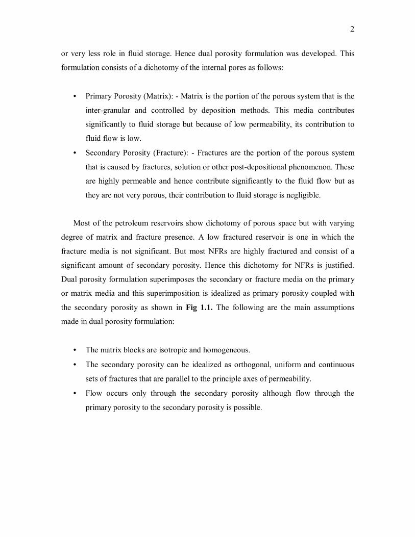
2
or very less role in fluid storage. Hence dual porosity formulation was developed. This
formulation consists of a dichotomy of the internal pores as follows:
• Primary Porosity (Matrix): - Matrix is the portion of the porous system that is the
inter-granular and controlled by deposition methods. This media contributes
significantly to fluid storage but because of low permeability, its contribution to
fluid flow is low.
• Secondary Porosity (Fracture): - Fractures are the portion of the porous system
that is caused by fractures, solution or other post-depositional phenomenon. These
are highly permeable and hence contribute significantly to the fluid flow but as
they are not very porous, their contribution to fluid storage is negligible.
Most of the petroleum reservoirs show dichotomy of porous space but with varying
degree of matrix and fracture presence. A low fractured reservoir is one in which the
fracture media is not significant. But most NFRs are highly fractured and consist of a
significant amount of secondary porosity. Hence this dichotomy for NFRs is justified.
Dual porosity formulation superimposes the secondary or fracture media on the primary
or matrix media and this superimposition is idealized as primary porosity coupled with
the secondary porosity as shown in Fig 1.1. The following are the main assumptions
made in dual porosity formulation:
• The matrix blocks are isotropic and homogeneous.
• The secondary porosity can be idealized as orthogonal, uniform and continuous
sets of fractures that are parallel to the principle axes of permeability.
• Flow occurs only through the secondary porosity although flow through the
primary porosity to the secondary porosity is possible.
3
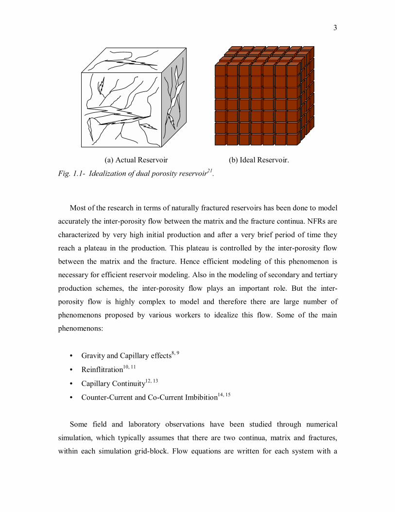
(a) Actual Reservoir (b) Ideal Reservoir.
Fig. 1.1- Idealization of dual porosity reservoir21.
Most of the research in terms of naturally fractured reservoirs has been done to model
accurately the inter-porosity flow between the matrix and the fracture continua. NFRs are
characterized by very high initial production and after a very brief period of time they
reach a plateau in the production. This plateau is controlled by the inter-porosity flow
between the matrix and the fracture. Hence efficient modeling of this phenomenon is
necessary for efficient reservoir modeling. Also in the modeling of secondary and tertiary
production schemes, the inter-porosity flow plays an important role. But the inter-
porosity flow is highly complex to model and therefore there are large number of
phenomenons proposed by various workers to idealize this flow. Some of the main
phenomenons:
• Gravity and Capillary effects8, 9
• Reinflitration10, 11
• Capillary Continuity12, 13
• Counter-Current and Co-Current Imbibition14, 15
Some field and laboratory observations have been studied through numerical
simulation, which typically assumes that there are two continua, matrix and fractures,
within each simulation grid-block. Flow equations are written for each system with a
4
matrix/fracture transfer function to relate the loss or gain of matrix fluids to or from the
fracture (inter-porosity flow). This fluid transfer rate is commonly calculated as a
function of the pressure difference between the matrix and fracture systems, matrix flow
capacity and matrix geometry considered through a constant shape factor. However, in
spite of the great level of current model sophistication, the highly anisotropy and
heterogeneous nature of a fractured formation makes fractured reservoir modeling a
challenging task, frequently with uncertain results in forecasting.
This study uses the counter-current imbibition phenomenon to model inter-porosity
flow. This model allows integration of the laboratory imbibition experiments and dual
porosity simulation to simulate fluid flow. This approach is shown to be an improved
way to model naturally fractured formations because it translates laboratory experiments
into inter-porosity flow. The definition of naturally fractured reservoirs can be extended,
without loss of generality, to any reservoir in which secondary porosity is significant16,17.
In this report the study has been divided into chapters. In chapter II, a detailed
literature review of the present models to simulate fluid flow in NFRs is presented.
Chapter III consists of derivation of the lab experiment modeling and integration of these
experiments with dual porosity formulations. Relevant equations are used to describe
both the numerical modeling of the imbibition experiments and also the proposed dual
porosity formulation. In chapter IV, imbibition experiments are modeled and the
extension to dual porosity formulations is tested using a commercially available
simulator. Chapter V details the conclusions derived from this study.
5
2
CHAPTER II
LITERATURE REVIEW
With increasing number of deep-water exploration, more number of fractured,
vuggular and heterogeneous reservoirs are being explored and developed. This has
increased the attention of the petroleum industry towards unconventional and fractured
reservoir modeling. With the advent of faster computers with large amount of memory
space, the industry is now able to model complex reservoirs faster and with much
accuracy. In this section, commonly used approaches for naturally fractured reservoir
modeling and inter-porosity flow estimation are reviewed and analyzed.
2.1 Fluid Flow Modeling in NFRs
Modeling of fluid flow in naturally fractured reservoirs can be broadly classified into
the following models7:
1. Discrete Fracture Network Models.
2. Equivalent Continuum Models.
3. Hybrid Models.
Discrete networks consist of modeling of a population of fractures. Equivalent
continuum methods, model reservoirs by assigning equivalent rock and fluid parameters
to large rock masses. Hybrid models are a combination of both discrete fracture networks
and equivalent continuum methods. The selection of any particular model depends, not
only on the reservoir and the type of fluid flow behavior to be numerically simulated, but
also on the amount of computer memory and speed available for the project. Due to the
ease of computation, the equivalent continuum modeling approach is the most favored to
model fluid flow in NFRs. But whenever models are to be solved very accurately with
very reliable data, the other two models may be applied. It has been shown that the
equivalent continuum methods are sufficient to model reservoir rocks that have
undergone multiple and extensive deformations (high fracture density) and/or any
formations where matrix permeabilities are large enough that fluid flow is not influenced
6
by any individual fracture or series of fractures that form a conducting channel18. Because
of the relevance to this study, the most important equivalent continuum models � single-
porosity and dual-porosity models � are briefly reviewed.
2.1.1 Single Porosity Modeling
Single porosity modeling is the most common method of modeling non-fractured
reservoirs. This model does not differentiate between the matrix and fracture continua
and equivalent rock and fluid properties are assigned to both the continuum. Since this
methodology doesn�t differentiate between the continua, this is the most accurate
modeling method. But its accuracy is dependent on the number of grid-blocks used
therefore can lead to large computational times.
Agarwal et al.19 have used the single continuum method to model a carbonate
reservoir with large number of fractures in the North Sea. To circumvent the problem of
computation, Agrawal used psuedo-relative permeability functions. To generate these
curves, dual porosity simulation was done on a stack of matrix blocks and matched with
fine grid simulation. This method receives special consideration because of the ease of
computation and accuracy generated by this methodology. This methodology, however,
cannot be used for reservoir management as new sets of dynamic pseudo-functions had to
be calculated for every change in operating conditions.
2.1.2 Dual Porosity Modeling
Dual porosity simulation is the most commonly used method for fluid flow modeling
in reservoirs with significant secondary porosity. In general, to model fluid flow in NFRs,
it is necessary to spatially define the secondary porosity. Since secondary porosity is
inherently complex and cannot be easily quantified, an idealization is made. This
idealization was initially proposed by Barenblatt et al.20 for single-phase fluid flow and
consisted of dividing the porous media in two superimposed continua, a continuous
continuum of fractures (secondary porosity) and a discontinuous matrix (primary
porosity) continuum. The fracture system is further assumed to be the primary flow paths
but have negligible storage capacity. Also the matrix is assumed to be the storage
medium of the system with negligible flow capacity. Warren and Root21 who presented
an analytical solution for the single-phase radial flow in a reservoir with significant

7
secondary introduced this idealization to the petroleum engineering. The idealization
made the following assumptions:
• The primary porosity is isotropic and is contained in a symmetric array of
identical parallelepipeds.
• All the secondary porosity is contained in a set of orthogonal fractures, which are
oriented in a direction parallel to the axis of permeability.
• Flow can occurs in the secondary porosity and from the primary porosity to the
secondary porosity but not in the primary porosity.
The idealization can be visualized as in Fig. 1.1. Both the primary and fracture media
are consistent in neither orientation nor continuity in Fig. 1.1 (a), which is the actual
reservoir. This actual reservoir is idealized as shown in Fig. 11 (b). The idealized
reservoir can be viewed as a series of primary porosity contained in the parallelepipeds,
which are disconnected from each other, by a series of continuous secondary porosities.
Other idealizations include parallel horizontal fracture22 and matchstick column4 models.
Multi-porosity models are a special case of dual porosity models, which assume that the
fracture set interacts with two groups of matrix blocks with distinct permeabilities and
porosities23.
2.2 Transfer Function
The primary and secondary porosities are coupled by a factor called the transfer
function or the inter-porosity flow. Physically, this can be defined as the rate of fluid flow
between the primary and the secondary porosities. Since the secondary porosity is the
only fluid path and it lacks in fluid storage, the dual porosity simulation method can be
imagined as a system of secondary porosity with the primary porosity as the only source
of fluids. The transfer function can be regarded as the �heart� of dual porosity since it is
the parameter that is changed to effect the transition from the actual reservoir as shown in
Fig. 1.1 (a) to the ideal reservoir as shown in Fig. 1.1 (b). Transfer functions can be
broadly classified to be of four types:
8
1. Empirical Transfer Functions.
2. Scaling Transfer Functions.
3. Diffusivity Transfer Functions.
4. Transfer Functions That Use Darcy Law.
2.2.1 Empirical Transfer Functions
Empirical models assume the transfer or inter-porosity flow can be attributed to
imbibition phenomenon. They assume an exponential decline function to describe the
time rate of exchange of oil and water for a single matrix block when surrounded by
fractures with high water saturation. Empirical transfer functions usually consist of two
parts:
1. A curve fitting expression to express recovery as a function of time.
2. A scaling equation to express the time in terms of rock and fluid properties.
The first empirical oil recovery function was given by Aronofsky24. He showed that
the rate of transfer of fluids from the matrix can be approximated by an exponential
decline function as shown
)1( teRR λ−∞ −= (2.1)
deSwaan25 used the above relation to derive an analytical expression for the water oil
ratio and the cumulative oil production from a linear reservoir with water flooding. His
theory also accounts for the fact that in a reservoir exploited by water flooding, the matrix
blocks downstream from the waterfront are subject to varying degree of saturation of
fractures due to the water imbibition of the matrix blocks upstream. His theory modifies
the well-known Buckley-Leverett formulation by addition of a term for the interporosity
flow or transfer function.
θθτ
φ τθ dSeNt
Shxq w
t
o
tmaw
∂∂+
∂∂=
∂∂− ∫ −− 1/)(
1
(2.2)
9
Also assuming that the fractional flow coefficient is the same as the mobile water
saturation, he derived an analytical solution for the above equation. The analytical
solution contains an integro-differential term as shown below.
>−<
=∫ −−
LFoyt
Lfw ttdytyIee
ttS
,)/2(1,0
/ ττ (2.3)
Kazemi et al.26 solved the analytical expression derived by deSwaan by using explicit
finite difference and trapezoidal rule. Reis and Cil27 proposed a new relation for oil
recovery function
( ) )1( 69.0 nteRR λ−∞ −= (2.4)
Civan28 extended the arfonsky relation by addition of an exponential term as shown in
equation 2.5.
)1( 21 tt eeRR λλ −−∞ −−= (2.5)
The second exponential term was justified by the fact that the collection of oil droplets in
the fracture consist of two different irreversible processes, namely:
1. Expulsion of oil droplets from the matrix into the fracture.
2. Entraining of the oil droplets in the fracture by the fluid present in the fracture.
The equation 2.5 was used in the Buckley-Leverett equation similar to deSwaan and a
numerical solution was developed. This numerical solution used the quadrature solution.
He showed that the quadrature solutions are easily computed than the finite difference
solutions for the case of end point mobilites. Civan and Gupta29 proposed an additional
term to the equation 2.5 as shown below
)1( 321 ttt eeeRR λλλ −−−∞ −−−= (2.6)
The third term was added to include the �dead-end� pores of the matrix but the results
obtained did not justify the need for the inclusion of this third term30. The above said
empirical methods suffer from the following limitations:
10
1. This method is limited to water flooded reservoirs.
2. The capillary pressure role in oil recovery is neglected.
3. Gravity is neglected.
4. This method is limited to two phases only.
2.2.2 Scaling Transfer Functions
Scaling transfer functions are used to predict recovery in field size cases with the results
from lab experiments. Rapoport31 proposed the �scaling laws� applicable in case of
water-oil flow. Using these laws Mattax and Kyte32 presented the dimensionless time to
scale up laboratory data to field size cases. The dimensionless time is given as
=
cwD L
ktt 2/µ
σφ (2.7)
Du Prey33 performed imbibition experiments on cores within centrifuges to account for
gravity effect on imbibition. He showed that the dimensionless time defined by the
previous equation couldn�t be used to model the experiments. He also showed that the
dimensionless equation 2.7 couldn�t be used for matrix blocks of different sizes. He
defined three more dimensionless parameters:
• Dimensionless Shape factor
• Dimensionless mobility
• Capillary to gravity ratio
The dimensionless time was defined for two cases: namely, low capillary to gravity ratio
and for high capillary to gravity ratio. His definitions are as follows
max
max
2
o
og
oct
oc
gkSHt
kPSHt
ρµφ
µφ
∆∆=
∆= (2.8)
Where
tc Dimensionless time factor for high capillary gravity ratio
11
tg Dimensionless time factor for low capillary gravity ratio
Ma et al.34 studied the relationship between water wetness and the oil recovery from
imbibition. The characteristic length to scale up time was also defined for various cases.
The authors also defined �effective viscosity� to remove the condition of comparable
viscosities between the lab and field cases.
2
1
cgD L
kttµσ
φ= (2.9)
Where
nwwg µµµ = (2.10)
Although the scaling transfer functions are the best transfer function representations, the
following are the requirements for the correct formulation of scaling transfer functions:
1. The shapes of the matrix blocks of the field and lab cases must be of the same
shape.
2. The fluid mobilites must be comparable.
3. The initial and boundary conditions for both the lab and matrix cases must be the
same.
4. The capillary pressures must be directly proportional
Because of these inherent assumptions the scaling transfer functions are not widely used.
2.2.3 Transfer Function Using Darcy�s Law
Transfer functions that use �Darcy�s Law�, assume that the transfer of fluids from the
matrix to the fracture can be adequately be described by Darcy�s law with an appropriate
geometric factor that accounts for the characteristic length and the flow area between the
matrix and the fracture.
The first model was proposed by Barenblatt et al. which is analgous to a model used
for heat transfer in a heterogeneous medium. They assumed that the outflow of fluids
from matrix blocks into the fractures is steady-state and that the fluid transfer rate is a
12
function of the viscosity of the fluid, the pressure drop between the matrix and fracture
systems, and matrix-rock properties related to geometry and porous interconnectivity in
the matrix block. According to Barenblatt et al., the fluid transfer rate per unit volume of
rock is calculated from the following expression:
)( fmm ppKq −=
µσ (2.11)
Where σ is a shape factor related to the specific surface of the fractures, pm and pf are
the average pressures in the matrix and fracture domains, respectively, and q is the fluid
transfer rate between the matrix and fracture. Although this transfer function is the most
popular, there is hardly any agreement between various researchers regarding the shape
factor. Bourbiaux et al.35 presented a comparison of shape factors found in the literature.
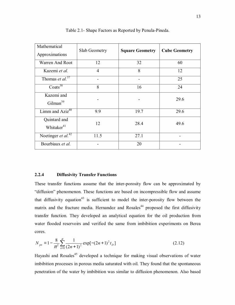
Table 2.1 is a modified version of the Bourbiaux table as reported by Penula-Pineda36.
Although the transfer functions of this family are the most popular they suffer from the
following limitations:
1. These assume a linear gradient of pressures between the matrix and the fractures
centers.
2. They also assume that the whole storage is present in the matrix blocks only.
3. These transfer functions lack a lab background that the other methods enjoy.
4. They also assume that all the matrix blocks exist at the same saturation.
5. Recovery from �n� number of matrix blocks is equal to �n� times the recovery
from a single matrix blocks.
6. Linear relative permeability is assumed in the fracture media.
13
Table 2.1- Shape Factors as Reported by Penula-Pineda.
Mathematical
Approximations Slab Geometry Square Geometry Cube Geometry
Warren And Root 12 32 60
Kazemi et al. 4 8 12
Thomas et al.37 - - 25
Coats38 8 16 24
Kazemi and
Gilman39 - - 29.6
Limm and Aziz40 9.9 19.7 29.6
Quintard and
Whitaker41 12 28.4 49.6
Noetinger et al.42 11.5 27.1 -
Bourbiaux et al. - 20 -
2.2.4 Diffusivity Transfer Functions
These transfer functions assume that the inter-porosity flow can be approximated by
�diffusion� phenomenon. These functions are based on incompressible flow and assume
that diffusivity equation43 is sufficient to model the inter-porosity flow between the
matrix and the fracture media. Hernandez and Rosales44 proposed the first diffusivity
transfer function. They developed an analytical equation for the oil production from
water flooded reservoirs and verified the same from imbibition experiments on Berea
cores.
])12(exp[)12(
181 2
022 D
npn tn
nN +−
+−= ∑
=
α
π (2.12)
Hayashi and Rosales45 developed a technique for making visual observations of water
imbibition processes in porous media saturated with oil. They found that the spontaneous
penetration of the water by imbibition was similar to diffusion phenomenon. Also based
14
on experimental results, a theoretical model is proposed for explaining imbibition
processes.
22
22
022 ])12(exp[
)12(18[1
LtnD
nN
npn
ππ
α +−+
−= ∑=
(2.13)
D is a coefficient to be estimated by trial and error.
The transfer functions of this family suffer from the following limitations:
1. They assume diffusion phenomenon is sufficient for inter-porosity flow.
2. This method can be used only for two-phase (water-oil) cases.
3. Compressibility of fluids is ignored.
2.2 Comparison of Transfer Functions
Reis and Cil27 have made comparisons between the various transfer functions on
several imbibition experiments with different boundary conditions and found the
following:
1. The match between the diffusivity models and the experimental data were found
to be good except at early times.
2. The scaling function was found to match the experiments within experimental
errors.
3. The empirical function was found to have a good agreement with the
experimental values.
For single-phase inter-porosity flow, Najurieta46 showed that deSwaan�s analytical model
results were equivalent to numerical solutions provided by Kazemi, which accounted for
pressure transient effects by assuming non-steady state flow at the matrix/fracture
interface.
The procedure developed in this study is intended for implementation in existing
simulators without significantly increasing computational work while representing
pressure transient and saturation gradient effects on the inter-porosity flow as accurately
15
as possible. In the following chapter, the conceptual model that is the basis for this
procedure is presented.
2.3 Flow Visualization Using X-ray Tomography
Computerized tomography is a non-destructive technique that utilizes X-rays and
mathematical reconstruction algorithms to generate a cross-sectional slice of an object47.
Hounsfield48 patented the first X-ray CT technique and was initially used for medical
purposes. The applications of X-ray CT in the petroleum industry have ranged from
detection of rock heterogenties49, 50,51 to determination of bulk densities52. But the main
use of CT has been found in flow visualization.
A detailed explanation of the principles and application of X-ray CT can be found
in the literature49.
16
3 CHAPTER III
FORMULATION OF MODELS
The objective of this chapter is to derive the formulations for:
1. Diffusivity Equations that are used to model imbibition experiments.
2. Derivation of empirical transfer function from imbibition experiments.
3.1 Derivation of the Diffusivity Equation
3.1.1 Conservation of Mass
From Darcy�s Law for multiphase flow in a porous media, we have that
)( ghpkkkku www
rww
w
rww ρ+∇
µ−=Φ∇
µ−=r
(3.1)
)( ghpkkkku ooo
roo
o
roo ρ+∇
µ−=Φ∇
µ−=r
(3.2)
From the definition of capillary pressure, the water phase pressure can be expressed in
terms of oil phase pressure as
)( wcwoc SPppP =−= ; cow Ppp −= (3.3)
Thus 3.1 can be re-written as
)( ghPpkku wcow
rww ρ
µ+−∇−=r (3.4)
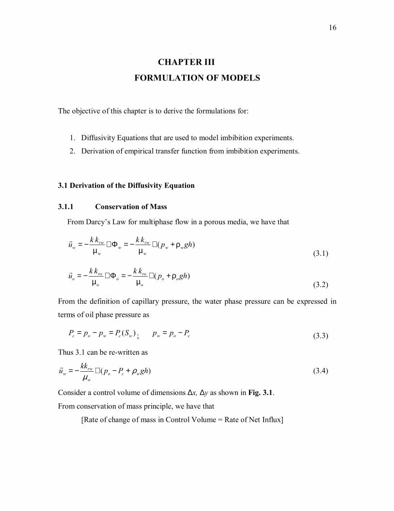
Consider a control volume of dimensions ∆x, ∆y as shown in Fig. 3.1.
From conservation of mass principle, we have that
[Rate of change of mass in Control Volume = Rate of Net Influx]
17
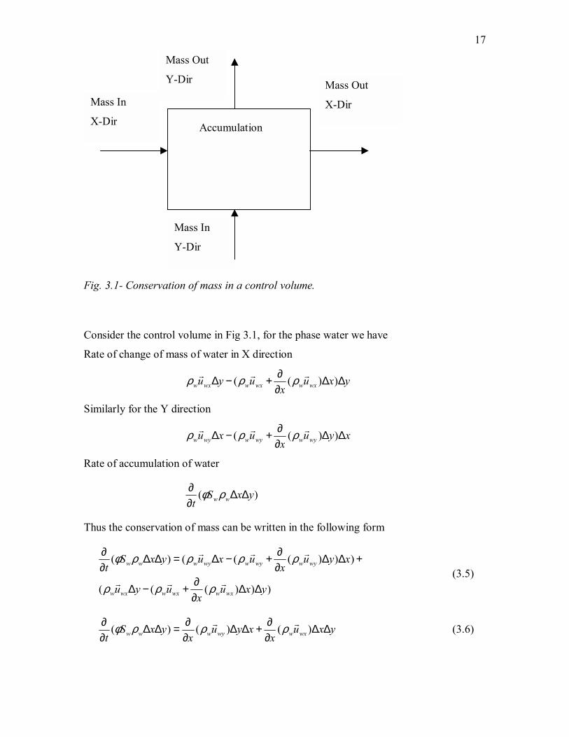
Fig. 3.1- Conservation of mass in a control volume.
Consider the control volume in Fig 3.1, for the phase water we have
Rate of change of mass of water in X direction
yxux
uyu wxwwxwwxw ∆∆∂∂+−∆ ))(( rrr ρρρ
Similarly for the Y direction
xyux
uxu wywwywwyw ∆∆∂∂+−∆ ))(( rrr ρρρ
Rate of accumulation of water
)( yxSt ww ∆∆
∂∂ ρφ
Thus the conservation of mass can be written in the following form
)))(((
)))((()(
yxux
uyu
xyux
uxuyxSt
wxwwxwwxw
wywwywwywww
∆∆∂∂+−∆
+∆∆∂∂+−∆=∆∆
∂∂
rrr
rrr
ρρρ
ρρρρφ (3.5)
yxux
xyux
yxSt wxwwywww ∆∆
∂∂+∆∆
∂∂=∆∆
∂∂ )()()( rr ρρρφ (3.6)
Mass In
Y-Dir
Mass In
X-Dir
Mass Out
Y-Dir Mass Out
X-Dir
Accumulation
18
yxux
xyux
yxSt wxwwywww ∆∆
∂∂+∆∆
∂∂=∆∆
∂∂ )()()( rr ρρρφ (3.7)
)()()( wxwwywww ux
ux
St
rr ρρρφ∂∂+
∂∂=
∂∂ (3.8)
).()( ww uSt
r∇=∂∂φ (3.9)
Similarly for oil phase we have
).()( oo uSt
r∇=∂∂φ (3.10)
Adding 1.9 and 1.10 we have
).()( wowo uuSSt
rr +∇=+∂∂φ (3.11)
But by definition we have that the sum of saturations is one. Therefore 3.11 can be
written as
0).( =+∇ wo uu rr (3.12)
3.1.2 Diffusivity Equation
Substituting equation 3.1 and 3.2 in 3.12 we have
0))()(.( =+∇−+−∇−∇ ghpkkghPpkkoo
o
rowco
w
rw ρµ
ρµ
(3.13)
Defining mobilites as
owTw
rww
o
roo
kkkk λλλµ
λµ
λ +=== ;; (3.14)
Substituting in 3.13 and rearranging terms we have
0))(.( =∇++∇−∇∇ hgPp wwoocwoT ρλρλλλ (3.15)
Now neglecting gravity terms we have
0).( =∇−∇∇ cwoT Pp λλ (3.16)

19
0).( =∇−∇∇ cT
wo Pp
λλ (3.17)
).().( cT
wo Pp ∇∇=∇∇
λλ (3.18)
From equation 3.10 we have that
).()( oo uSt
r∇=∂∂φ (3.19)
).()( ooo pSt
∇∇=∂∂ λφ (3.20)
).()( oow pSt
∇∇=∂∂− λφ (3.21)
)(.()( CT
wow PS
t λλλφ ∇∇=
∂∂− ) (3.22)
0)().( =∂∂+∇∇ wC
T
wo St
P φλλλ (3.23)
0)().( =∂∂+∇∇ ww
w
C
T
wo St
SdSdP φ
λλλ (3.24)
0)().( =∂∂+∇∇ ww St
SD (3.25)
Where
D = w
c
T
wo
dSdP)(
φλλλ +
3.1.3 Discretization of the Diffusivity Equation
3.1.3.1 Initial and Boundary Conditions
Equation 3.25 is the final form of the diffusivity equation. In order to simulate the
core imbibition experiments, boundary and initial conditions are required. The following
are the initial and boundary conditions used.
20
Initial Condition
0,1),,( =−= tStyxS oiw (3.26)
Boundary Condition
Depending on the boundaries modeled the boundary condition as shown below
can be utilized. For example if the core is completely surrounded by the wetting phase
then the boundary condition would be
xw
yw
w
w
LxtyxS
LytyxSytyxSxtyxS
==
======
,1),,(
,1),,(0,1),,(0,1),,(
(3.27)
And if the core is surrounded by the wetting phase only at the bottom as in Garg et al.
case then the boundary conditions are as follows
0,1),,( == ytyxSw (3.28)
3.1.3.2 Finite Difference Form of Diffusivity Equation
Consider a spatial control volume that has been divided into a mesh of grid blocks
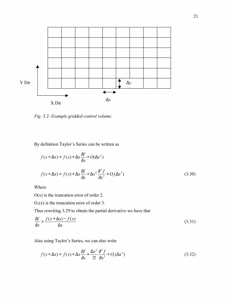
of equal dimensions ∆ x. and ∆ y (two dimensions) as shown in Fig. 3.2. So the objective
of this exercise is to discretize equation 1.25 on this control volume.
21
Fig. 3.2- Example gridded control volume.
By definition Taylor�s Series can be written as
)()()( 2xOxfxxfxxf ∆+
∂∂∆+=∆+
)()()( 313
22 xO
xfx
xfxxfxxf ∆+
∂∂∆+
∂∂∆+=∆+ (3.30)
Where
O(x) is the truncation error of order 2.
O1(x) is the truncation error of order 3.
Thus rewriting 3.29 to obtain the partial derivative we have that
xxfxxf
xf
∆−∆+=
∂∂ )()( (3.31)
Also using Taylor�s Series, we can also write
)(!2
)()( 313
22
xOxfx
xfxxfxxf ∆+
∂∂∆+
∂∂∆+=∆+ (3.32)
X Dir
Y Dir
x∆
y∆
22
)(!2
)()( 312
22
xOx
fxxfxxfxxf ∆+
∂∂∆+
∂∂∆−=∆− (3.33)
adding 3.33 and 3.34 we have that
)(!2
2)(2)()( 312
22
xOxfxxfxxfxxf ∆+
∂∂∆+=∆++∆− (3.34)
22
2 )(2)()(x
xfxxfxxfxf
∆−∆−+∆−=
∂∂ (3.35)
Thus from equation 3.31 we have that
tSS
tS n
wn
ww
∆−=
∂∂ +1
(3.36)
Where
n Time step
n + 1 Incremented time step
Also,
ySS
ySS
yS
xSS
xSS
xS
jwwjjwjww
iwwiiwiww
∆−
=∆
−=
∂∂
∆−
=∆
−=
∂∂
−+
−+
11,
11,
(3.37)
Where
i Grid Block Number in X Direction
j Grid Block Number in Y direction
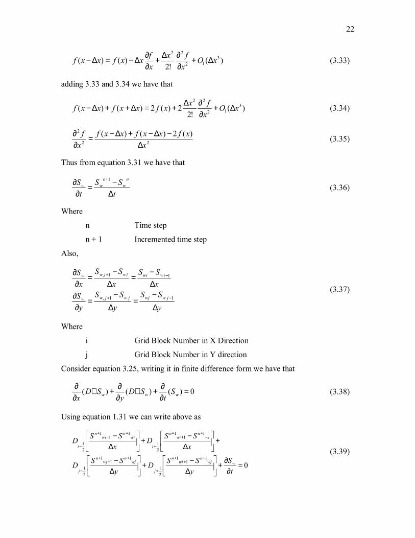
Consider equation 3.25, writing it in finite difference form we have that
0)()()( =∂∂+∇
∂∂+∇
∂∂
www St
SDy
SDx
(3.38)
Using equation 1.31 we can write above as
01
11
21
11
1
21
11
1
21
11
1
21
=∂
∂+
∆−+
∆−
+
∆−+
∆−
++
+
+
+−
+
−
++
+
+
+−
+
−
tS
ySSD
ySSD
xSSD
xSSD
wwjn
wjn
j
wjn
wjn
j
win
win
i
win
win
i (3.39)
23
Where
i-1/2, i+1/2, j-1/2, j+1/2 are the averaged values of D as explained in the next section.
Using equation 3.36, 3.39 can be transformed as
011
11
21
11
1
21
11
1
21
11
1
21
=
∆−+
∆
−+
∆
−
+
∆
−+
∆
−
+++
+
+
+−
+
−
++
+
+
+−
+
−
tSS
ySSD
ySSD
xSSD
xSSD
nw
nwwj
nwj
n
j
wjn
wjn
j
win
win
i
win
win
i (3.40)
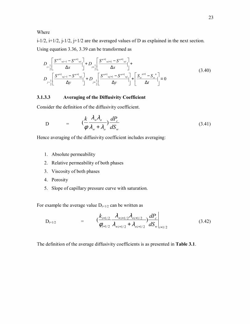
3.1.3.3 Averaging of the Diffusivity Coefficient
Consider the definition of the diffusivity coefficient.
D = w
c
ow
ow
dSdPk )(
λλλλ
φ + (3.41)
Hence averaging of the diffusivity coefficient includes averaging:
1. Absolute permeability
2. Relative permeability of both phases
3. Viscosity of both phases
4. Porosity
5. Slope of capillary pressure curve with saturation.
For example the average value Di+1/2 can be written as
Di+1/2 = 2/12/12/1
2/12/1
2/1
2/1 )(+++
++
+
+
+iw
c
ioiw
ioiw
i
i
dSdPk
λλλλ
φ (3.42)
The definition of the average diffusivity coefficients is as presented in Table 3.1.
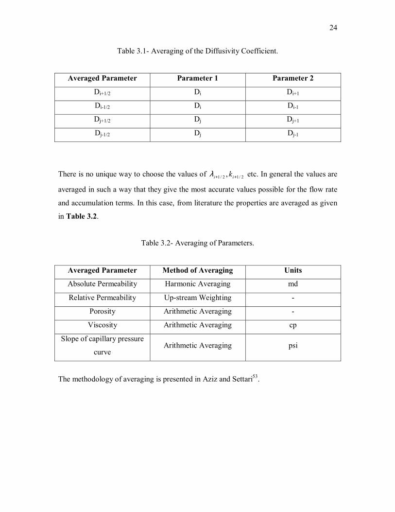
24
Table 3.1- Averaging of the Diffusivity Coefficient.
Averaged Parameter Parameter 1 Parameter 2
Di+1/2 Di Di+1
Di-1/2 Di Di-1
Dj+1/2 Dj Dj+1
Dj-1/2 Dj Dj-1
There is no unique way to choose the values of 2/12/1 , ++ ii kλ etc. In general the values are
averaged in such a way that they give the most accurate values possible for the flow rate
and accumulation terms. In this case, from literature the properties are averaged as given
in Table 3.2.
Table 3.2- Averaging of Parameters.
Averaged Parameter Method of Averaging Units
Absolute Permeability Harmonic Averaging md
Relative Permeability Up-stream Weighting -
Porosity Arithmetic Averaging -
Viscosity Arithmetic Averaging cp
Slope of capillary pressure
curve Arithmetic Averaging psi
The methodology of averaging is presented in Aziz and Settari53.
25
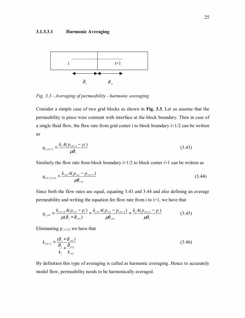
3.1.3.3.1 Harmonic Averaging
Fig. 3.3 - Averaging of permeability - harmonic averaging.
Consider a simple case of two grid blocks as shown in Fig. 3.3. Let us assume that the
permeability is piece wise constant with interface at the block boundary. Then in case of
a single fluid flow, the flow rate from grid center i to block boundary i+1/2 can be written
as
i
iiiii
ppAkq∂
−= ++ µ
)( 2/12/1, (3.43)
Similarly the flow rate from block boundary i+1/2 to block center i+1 can be written as
1
2/1111,2/1
)(
+
+++++ ∂
−=i
iiiii
ppAkqµ
(3.44)
Since both the flow rates are equal, equating 3.43 and 3.44 and also defining an average
permeability and writing the equation for flow rate from i to i+1, we have that
i
iii
i
iii
ii
iiiii
ppAkppAkppAkq∂
−=∂
−=∂+∂
−= +
+
+++
+
+++ µµµ
)()()(
)( 2/1
1
2/111
1
12/11, (3.45)
Eliminating p i+1/2 we have that
1
1
12/1
)(
+
+
++ ∂+∂
∂+∂=
i
i
i
i
iii
kk
k (3.46)
By definition this type of averaging is called as harmonic averaging. Hence to accurately
model flow, permeability needs to be harmonically averaged.
i i+1
i∂ +∂ i
26
3.1.3.3.2 Arithmetic Averaging
The pressure dependent properties are assumed to be arithmetic averaged since
these properties are not variable in the present case. The pressure is constant for the
length of the imbibition experiment.
The capillary pressure curve slope is assumed to be arithmetic averaged54.
3.1.3.3.3 Upstream Weighting
Upstream weighting of relative permeability and capillary pressure is a
consequence of the hyperbolic nature of the problem. Raithby55 showed that the upstream
weighting leads to an accurate solution. The upstream weighting is defined as follows.
)( wirlrw Skk = if flow is from i to i+1.
and rwk = )( 1+wirw Sk if flow is from i+1 to i.
3.2 Derivation of Dual Porosity Flow Equations
3.2.1 Flow Equations
3.2.1.1 Fracture Flow Equations
Stating Darcy�s Law for multiphase flow in porous media, we have
)( ghpkkkku www
rww
w
rww ρ+∇
µ−=Φ∇
µ−=r
(3.47)
)( ghpkkkku ooo
roo
o
roo ρ+∇
µ−=Φ∇
µ−=r
(3.48)
Since the primary flow path in dual porosity formulation is the fracture we have the
Darcy�s Law as follows
)( ghpB
kku wwf
wfwf
rwffwf ρ
µ+∇−=r (3.49)
)( ghpB
kku oof
ofof
roffof ρ
µ+∇−=r (3.50)

27
From the definition of capillary pressure, the water phase pressure can be expressed in
terms of oil phase pressure as
)( wcwoc SPppP =−= ; cow Ppp −= (3.51)
Thus 3.47 can be re-written as
)( ghPpB
kku wcfof
wfwf
rwffwf ρ
µ+−∇−=r (3.52)
Consider a control volume (Secondary Porosity) of dimensions ∆x, ∆y as shown
in Fig. 3.1. For the sake of brevity the subscript f is dropped in the derivation of the
conservation of mass.
From conservation of mass principle, we have that
[Rate of change of mass in Control Volume = Rate of Net Influx]
Consider the control volume in figure 3.1, for the phase water we have
• Rate of change of mass of water in X direction
yxux
uyu wxwwxwwxw ∆∆∂∂+−∆ ))(( rrr ρρρ
• Similarly for the Y direction
xyux
uxu wywwywwyw ∆∆∂∂+−∆ ))(( rrr ρρρ
• Rate of accumulation of water
τρφ +∆∆∂∂ )( yxSt ww
Where τ is the rate of flow of water from the matrix to the fracture, since the primary
porosity also contributes to the accumulation of water in the fractures. Thus the
conservation of mass can be written in the following form
28
)))(((
)))((()(
yxux
uyu
xyux
uxuyxSt
wxwwxwwxw
wywwywwywww
∆∆∂∂+−∆
+∆∆∂∂+−∆=+∆∆
∂∂
rrr
rrr
ρρρ
ρρρτρφ (3.53)
Simplifying equation 3.53 similar to the conservation of mass as described in the earlier
chapter we have,
).()( www uSt
r∇=+∂∂ τφ (3.54)
Similarly for oil phase we have
).()( ooo uSt
r∇=+∂∂ τφ (3.55)
Substituting equations 3.50 and 3.49 in equations 3.54 and 3.55 we have that
))(.()( ghPpB
kkS
t wcfofwfwf
rwffwwf ρ
µτφ +−∇−∇=+
∂∂ (3.56)
))(.()( ghpB
kkS
t oofofof
roffoof ρ
µτφ +∇−∇=+
∂∂ (3.57)
We know that the sum of the saturations is unity. Hence
tS
tSSSSS wo
wowo ∂∂−=
∂∂−==+ ;1;1 (3.58)
Simplifying equation 3.60 and 3.61 and using 3.62 in 3.61 we have that
))(.()( ghpB
kkS
t oofofof
roffowf ρ
µτφ +∇−∇=+
∂∂− (3.59)
))(.()( ghPpB
kkS
t wcfofwfwf
rwffwwf ρ
µτφ +−∇−∇=+
∂∂ (3.60)
Multiplying both sides of the equation by the bulk volume we have
))(.()( ghpaVSt
V oofoobwfp ρτ +∇∇=−∂∂ (3.61)
29
))(.()( ghPpaVSt
V wcfofwwbwfp ρτ +−∇∇=−∂∂− (3.62)
Where
a Symmetric coefficient defined as
aw bwfwf
rwff VB
kkµ
The above equations don�t consider source and sink terms like injection wells,
production wells etc. To include wells into equation 3.65 and 3.66 the flow rate is added
to the RHS with the convention of positive for production and negative in case of an
injector. Therefore equations 3.65 and 3.66 can be rewritten as
))(.()( ghpaqVSt
V oofooobwfp ρτ +∇∇=−−∂∂ (3.63)
))(.()( ghPpaqVSt
V wcfofwwwbwfp ρτ +−∇∇=−−∂∂− (3.64)
3.2.1.2 Matrix Flow Equations
Consider a control volume of matrix similar to fig. 3.1. The rate of inflow into the
matrix is zero as there is no flow into the matrix while the rate of outflow from the matrix
into the transfer function, the conservation of mass can be written as
)(0 St
φτ∂∂=− (3.65)
wmaw St
)(φτ∂∂=− (3.66)
omao St
)(φτ∂∂=− (3.67)
3.2.2 Empirical Transfer Function
The empirical equations are derived from the imbibition experiments that are
conducted on the matrix core. To scale the time from the imbibition experiments to the
field size Mattax and Kyte proposed the following transformation.
30
kmatrixblocwelw
kL
tkL
t
=
φµσ
φµσ
2mod
2 (3.68)
Therefore time can be converted to dimensionless time as
=
φµσ k
Ltt
wD 2 (3.69)
From the imbibition data, a table of the recovery versus time is already obtained.
Converting the time from the imbibition experiments to dimensionless as given by
equation 3.50, and also the recovery can be converted into dimensionless form using the
following equation
RD V
RR = (3.70)
Therefore, from the numerical simulation of the imbibition experiment, a table of the
recovery and time in dimensionless units can be obtained. Now the problem resolves in
expressing the dimensional recovery in terms of the transfer function.
3.2.2.1 Expression of Transfer Function in Terms of Imbibition Recovery
DeSwaan proposed that the rate of imbibition into the fracture from the matrix could
be expressed as
εε
λτ λεα d
SeR wf
t
o
tD
∂∂
= ∫ −− )( (3.71)
He also derived the Buckley-Leverett solution for the 1-D, 2-Phase water flooding
displacement process. Considering the integral as shown above, the transfer function can
be written as
∑ ∏= =
∆−+
−=n
j
n
jk
tjwfjwf
ketStSR0
1 )]()([ λα λτ (3.72)
Simplifying equation 3.76 we have
31
{ }1 Dntn eSumR ∆−−= λα λτ (3.73)
Where
1)( 121 −∆−−−− −+= Dntnwf
nwf
nn eSSSumSum λ
3.2.2.2 Implementation of Transfer Function in Terms of Recovery
Equation 3.65 and 3.66 combined with equation 3.77 can be written as
{ ))(.(})( 1 ghpaqeSumRSt
V oofootn
wfpDn ρλ λ
α +∇∇=−−∂∂− ∆−−∑ (3.74)
{ ))(.(})( 1 ghPpaqeSumRSt
V wcfofwwtn
wfpDn ρλ λ
α +−∇∇=−−∂∂ ∆−−∑ (3.75)
Therefore now the problem is reduced to a two-unknown two-equation problem.
3.2.3 Discretization of the Equations
Equation 3.67 and 3.68 can be discretized as shown in the previous chapter using the
finite difference technique and the following equation can be arrived
{ eSumR qStBV
a Dntnow
opoo }
/ - = 1 ∆−−∑++
∆Φ∆∆ λα λδ (3.76)
{ eSumR qSwtBV
a Dntnw
wpww }
/ = 1 ∆−−∑++
∆Φ∆∆ λα λδ (3.77)
Where
a Symmetric Coefficient
Φ Potential. Defined as
∆ Φ w ∆ (p-Pc) - Hgw ∆ρ
∆ Φ o ∆ (p) - Hgo ∆ρ
Operator ∆ Defined as
yx ∂∂+
∂∂=∆ (3.78)
32
Writing the equations 3.81 and 3.82 after finite difference discretization, neglecting
gravity we have
{ eSumRqSwSwt
BVaaaa
Dntno
nnop
nj
nj
noN j
nj
nj
noS j
ni
ni
noE i
ni
ni
now i
} + ) - ( /
- =
) - ( + ) - ( ) - ( + ) - (
11+
1+1+1+
1+1+1+1-
1+1+1+1+
1+1+1+1-
1+1-
∆−−∑+∆
ΦΦΦΦ+ΦΦΦΦ
λα λ
{ eSumRqSwSw
tBV
aaaa
Dntnw
nnwp
nj
nj
nwN j
nj
nj
nwS j
ni
ni
nwE i
ni
ni
nww i
} + ) - ( /
=
) - ( + ) - ( ) - ( + ) - (
11+
1+1+1+
1+1+1+1-
1+1+1+1+
1+1+1+1-
1+1-
∆−−∑+∆
ΦΦΦΦ+ΦΦΦΦ
λα λ
(3.79)
The equations 3.83 and 3.84 are highly non-linear. With the advent of faster computers
the conventional IMPES formulation of the above equation is not necessary as the
IMPES method are known for their stability problems. Hence the fully implicit option is
applied. To solve the equations mentioned, Newton-Raphson�s method of solution can be
applied.
3.2.3.1 Newton-Raphson�s Solution of Non-Linear Equations
Consider equations 3.83 and 3.84. They can be posed in the matrix form as shown
below
bXArrr
= (3.80)
Where
Φ
Φ
=
wf
f
wf
f
S
S
X..r
Ar
Coefficient Matrix
33
br
Right Hand Side Matrix
Since both �A� and �b� matrices in 3.85 are functions of �X� matrix the system of
equations is non-linear. Rewriting the equation
bXARrrrr
−= (3.81)
Where R matrix is called the residual matrix. Using the Taylor�s series expansion the
residual matrix can be written as
)( 11 nn
n
nn xxxRRR rrr
rr−
∂∂+= ++ (3.82)
Setting Rn+1 to zero as the objective is to reduce the residual to zero, the following
equation can be derived
1+∆
∂∂−= k
k
k xxRR rr
r (3.83)
Where
∆ xk+1 xk+1-xk
k Iteration counter
Equation 3.88 is similar to 3.86. Therefore the equations 3.83 and 3.84 can be posed in
the form of residuals and the partial derivative in the equation 3.88 can be computed as
the coefficient of the change in residual with respect to a variable and the difference
matrix is to be computed.
In order to solve equation 3.88 at the beginning of every time step the value of the
iteration counter is made to unity and the residuals are computed at the previous time
step. Then the Jacobian matrix or the partial derivative is computed at the iteration level.
The equation 3.88 is solved. With the new difference matrix, the variables is updated and
checked for convergence. If not converged, the iteration counter is incremented and the
process is repeated till convergence. A flow diagram is presented in Fig. 3.4.
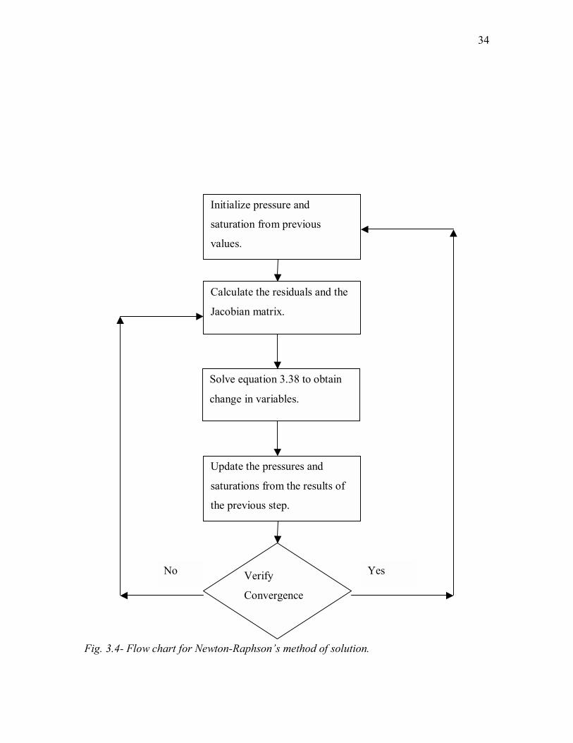
34
Fig. 3.4- Flow chart for Newton-Raphson�s method of solution.
Initialize pressure and
saturation from previous
values.
Calculate the residuals and the
Jacobian matrix.
Solve equation 3.38 to obtain
change in variables.
Update the pressures and
saturations from the results of
the previous step.
Verify
Convergence
Yes No
35
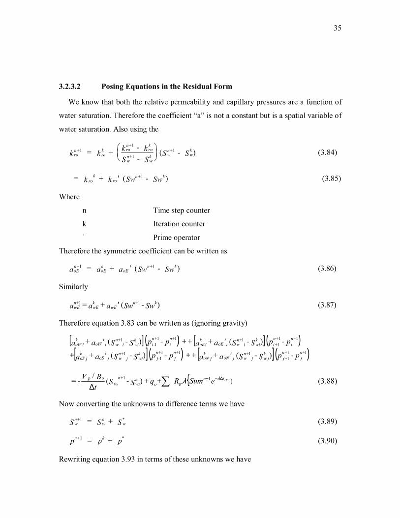
3.2.3.2 Posing Equations in the Residual Form
We know that both the relative permeability and capillary pressures are a function of
water saturation. Therefore the coefficient �a� is not a constant but is a spatial variable of
water saturation. Also using the
ron
rok ro
nrok
wn
wk w
nwkk k k k
S SS S +
+
++ = +
- -
( - )11
11
(3.84)
= + ( - )+kro ro
n kk k Sw Sw′ 1 (3.85)
Where
n Time step counter
k Iteration counter
` Prime operator
Therefore the symmetric coefficient can be written as
oEn
oEk
oEn ka a a Sw Sw + + = + ( - )1 1′ (3.86)
Similarly
SwSwaaa knwE
kwE
nwE ) - ( + = 1+1+ ′ (3.87)
Therefore equation 3.83 can be written as (ignoring gravity)
[ ] ( ) [ ] ( )[ ] ( ) [ ] ( )ppSSaa ppSSaa
ppSSaa ppSSaanj
nj
kw j
nw joN j
koN j
nj
nj
kwi
nw joS j
koS j
ni
ni
kwi
nw ioE i
koEi
ni
ni
kwi
nw ioW i
koW i
1+1+1+
1+1+1+1-
1+
1+1+1+
1+1+1+1-
1+
- ) - ( + + - ) - ( +
- ) - ( + + - ) - ( +
′+′+
′+′
{ eSumRqSStBV Dn
i
tno
nwiw
nop } + ) - ( /
- = 11+ ∆−−∑+∆
λα λ (3.88)
Now converting the unknowns to difference terms we have
wn
wk
wS S S+ * = + 1 (3.89)
n kp p p+ * = + 1 (3.90)
Rewriting equation 3.93 in terms of these unknowns we have
36
[ ] ( ) [ ] ( )[ ] ( ) [ ] ( )ppppSaa ppppSaa
ppppSaa ppppSaa
jjkj
kjw joN j
koN jjj
kj
kjw joS j
koS j
iiki
kiwioE i
koEiii
ki
kiwioW i
koW i
**1+1+
***1+1-
*
**1+1+
***1-1-
*
- - + - - +
- - + - - +
+′++′+
+′++′
{ eSumRqSSStBV Dn
i
tno
nwiwiw
kop } + ) - ( /
- = 1* ∆−−∑++∆
λα λ (3.91)
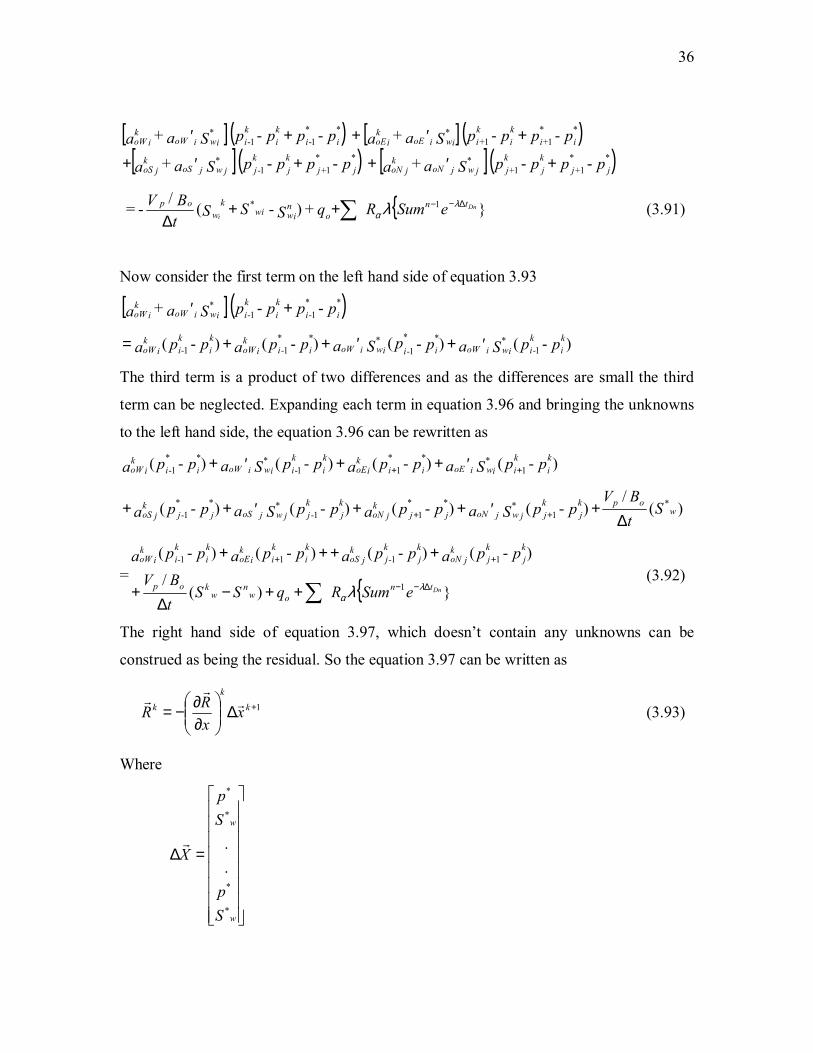
Now consider the first term on the left hand side of equation 3.93
[ ] ( )ppppSaa iiki
kiwioW i
koW i
**1-1-
* - - + +′
) - ( ) - ( ) - () - ( 1-*** *
1-**
1-1- ppSappSappappaki
kiwioW iiwioW i iii
koW i
ki
ki
koW i ′+′++=
The third term is a product of two differences and as the differences are small the third
term can be neglected. Expanding each term in equation 3.96 and bringing the unknowns
to the left hand side, the equation 3.96 can be rewritten as
) - ( ) - () - ( ) - ( 1***
11-***
1- ppSappappSappaki
kiwioE iii
koEi
ki
kiwioW iii
koW i ++ ′++′+
)(/
) - ( ) - () - ( ) - ( *1
***11-
***1- w
opkj
kjw joN jjj
koN j
kj
kjw joS jjj
koS j S
tBV
ppSappappSappa ∆+′++′++ ++
={ })(
/
) - () - () - () - (
1
11-11-
Dntnow
nw
kop
kj
kj
koN j
kj
kj
koS j
ki
ki
koEi
ki
ki
koW i
eSumRqSStBV
ppappappappa
∆−−
++
∑++−∆
+
++++
λα λ
(3.92)
The right hand side of equation 3.97, which doesn�t contain any unknowns can be
construed as being the residual. So the equation 3.97 can be written as
1+∆
∂∂−= k
k
k xxRR rr
r (3.93)
Where
=∆
w
w
Sp
Sp
X
*
*
*
*
.
.r
37
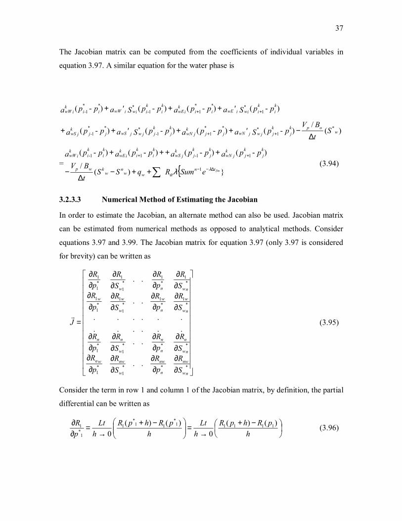
The Jacobian matrix can be computed from the coefficients of individual variables in
equation 3.97. A similar equation for the water phase is
) - ( ) - () - ( ) - ( 1***
11-***
1- ppSappappSappaki
kiwiwE iii
kwEi
ki
kiwiwW iii
kwW i ++ ′++′+
)(/
) - ( ) - () - ( ) - ( *1
***11-
***1- w
opkj
kjw jwN jjj
kwN j
kj
kjw jwS jjj
kwS j S
tBV
ppSappappSappa ∆−′++′++ ++
={ })(
/
) - () - () - () - (
1
11-11-
Dntnww
nw
kwp
kj
kj
kwN j
kj
kj
kwS j
ki
ki
kwEi
ki
ki
kwW i
eSumRqSStBV
ppappappappa
∆−−
++
∑++−∆
−
++++
λα λ
(3.94)
3.2.3.3 Numerical Method of Estimating the Jacobian
In order to estimate the Jacobian, an alternate method can also be used. Jacobian matrix
can be estimated from numerical methods as opposed to analytical methods. Consider
equations 3.97 and 3.99. The Jacobian matrix for equation 3.97 (only 3.97 is considered
for brevity) can be written as
∂∂
∂∂
∂∂
∂∂
∂∂
∂∂
∂∂
∂∂
∂∂
∂∂
∂∂
∂∂
∂∂
∂∂
∂∂
∂∂
=
***1
*1
***1
*1
*1
*1
*1
1*1
1
*1
*1
*1
1*1
1
..
..............
..
..
nw
nw
n
nw
w
nwwn
nw
n
n
n
w
nn
nw
w
n
w
w
ww
nwnw
SR
pR
SR
pR
SR
pR
SR
pR
SR
pR
SR
pR
SR
pR
SR
pR
Jr
(3.95)
Consider the term in row 1 and column 1 of the Jacobian matrix, by definition, the partial
differential can be written as
−+
→=
−+→
=∂∂
hpRhpR
hLt
hpRhpR
hLt
pR )()(
0)()(
011111
*11
*1
1*1 (3.96)

38
The user can specify the value of �h� in the above equation and the limit of the ratio can
be approximated as the ratio. Since the residual is continuous at zero. Therefore the
partial differential can be written as
−+=
∂∂
hpRhpR
pR )()( 1111
1*1 (3.97)
Writing similarly for all the elements in the Jacobian matrix.
3.2.3.4 Method of Solution of the System of Equations
To solve the system of equations as posed by equation 3.98 for both the water and the oil
phases, the Gaussian elimination method is proposed. Gaussian elimination is briefly
described in this section.
To solve a system of equations as shown below,
=++
=++=++
nnnnnn
nn
nn
bxaxaxa
bxaxaxabxaxaxa
...................
2211
22222121
11212111
(3.98)
Gaussian elimination�s objective is to rewrite the above equation in the following form
=
=+=++
nnnn
nn
nn
x
xxxxx
βα
βααβααα
.......
......
22222
11212111
(3.99)
To obtain this transformation the following matrix rules are applied:
1. Interchanging of the order of the equations.
2. Multiplication of any equation by a non-zero number.
3. Addition of any equation with a multiple of any other.
After the system of equations is posed in the form indicated by 3.104, the value of
xn is first calculated using the last equation of the system, then xn-1 and so on till x1 is
calculated. To effect the above transformation the following method or algorithm is used:

39
1. Starting with the first equation, divide the equation by a11 to get one in the
first term.
2. Subtract a1i times the first equation from all the equations below the first
equation to make the first term in all those equations zero.
3. Repeat the step for the second equation and so on till the last equation consists
of only one term.
40
4
CHAPTER IV
DISCUSSION AND RESULTS
The objective of this chapter is to present results from the numerical models
presented in the previous chapters. The results are divided into two parts:
1. The results from the imbibition experiments
2. The results from the dual porosity simulation using empirical transfer functions.
4.1 Imbibition Experiments
The formulations derived in Chapter III were used to numerically simulate the imbibition
experiments of the following workers:
• Garg et al.58
• Muralidharan59
4.1.1 Garg Imbibition Experiment
4.1.1.1 Brief Description of Garg et al. Imbibition Experiment
Garg et al. performed a one-dimensional imbibition study on a Berea sandstone
core. The properties of the core are provided in Table 4.1. The core was heated at 7500 C
to remove the effects of clay swelling and migration during the imbibition experiment.
The core was epoxied on the sides so that imbibition occurs only from bottom to top. The
fluid used was normal tap water at room temperature. The schematic of the experiment is
presented in Fig. 4.1 The Berea core was suspended from a weight balance using a steel
wire into an acrylic container. The container is connected to a water tank through a
rubber tube. The weight balance is connected to a data acquisition system that reads the
weight of the core every second.
The water level in the container is always maintained at the bottom of the core.
The weight data was acquired for 120 minutes.
41
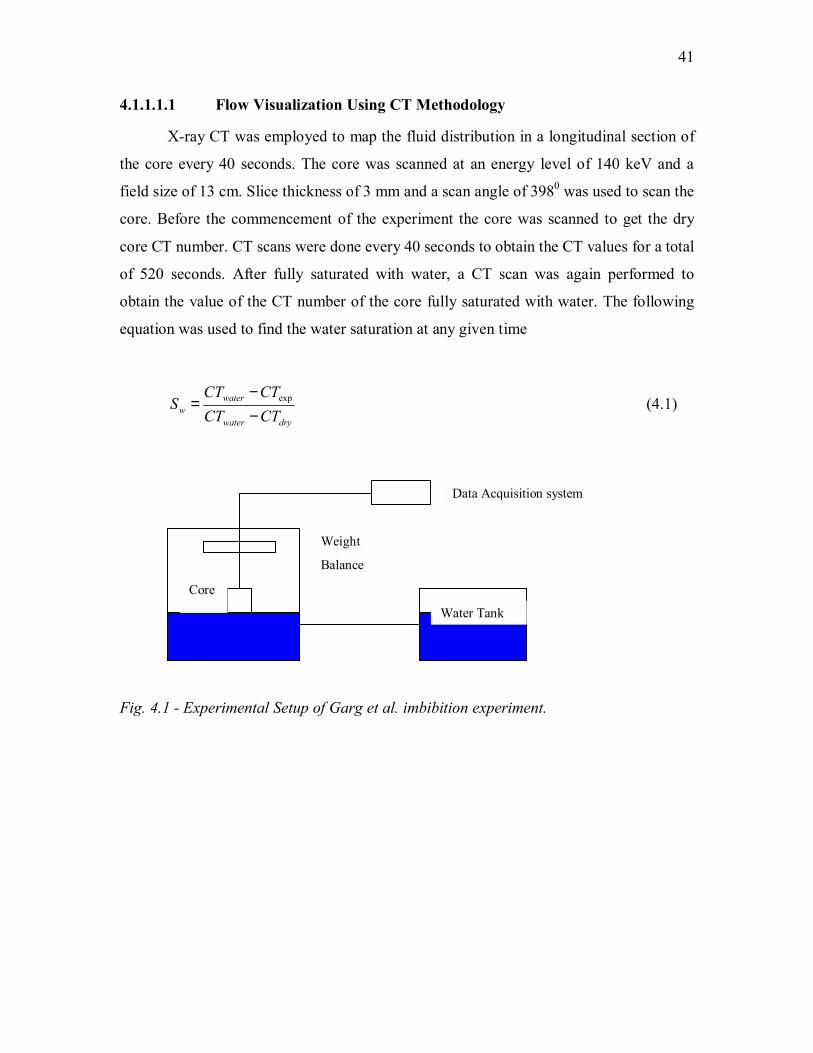
4.1.1.1.1 Flow Visualization Using CT Methodology
X-ray CT was employed to map the fluid distribution in a longitudinal section of
the core every 40 seconds. The core was scanned at an energy level of 140 keV and a
field size of 13 cm. Slice thickness of 3 mm and a scan angle of 3980 was used to scan the
core. Before the commencement of the experiment the core was scanned to get the dry
core CT number. CT scans were done every 40 seconds to obtain the CT values for a total
of 520 seconds. After fully saturated with water, a CT scan was again performed to
obtain the value of the CT number of the core fully saturated with water. The following
equation was used to find the water saturation at any given time
drywater
waterw CTCT
CTCTS
−−
= exp (4.1)
Fig. 4.1 - Experimental Setup of Garg et al. imbibition experiment.
Water Tank
Core
Weight
Balance
Data Acquisition system
42
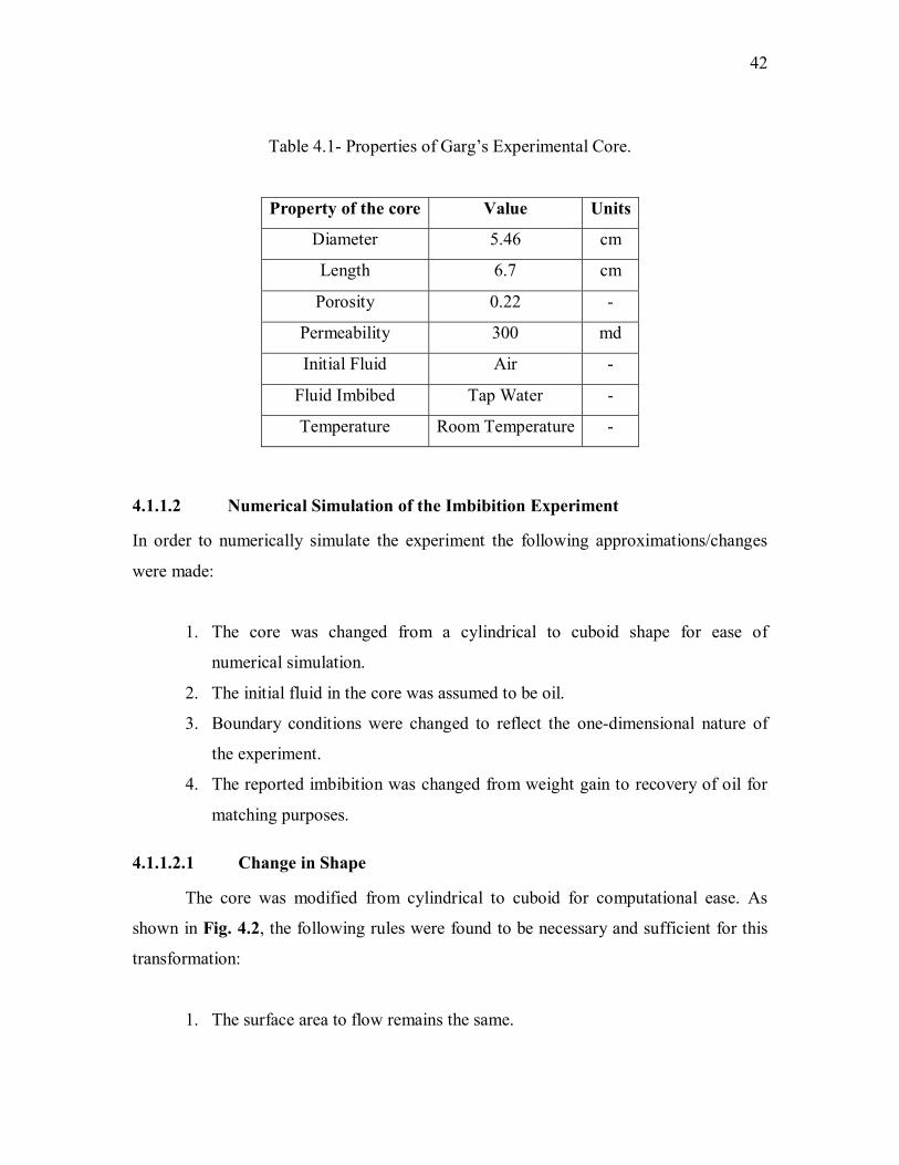
Table 4.1- Properties of Garg�s Experimental Core.
Property of the core Value Units
Diameter 5.46 cm
Length 6.7 cm
Porosity 0.22 -
Permeability 300 md
Initial Fluid Air -
Fluid Imbibed Tap Water -
Temperature Room Temperature -
4.1.1.2 Numerical Simulation of the Imbibition Experiment
In order to numerically simulate the experiment the following approximations/changes
were made:
1. The core was changed from a cylindrical to cuboid shape for ease of
numerical simulation.
2. The initial fluid in the core was assumed to be oil.
3. Boundary conditions were changed to reflect the one-dimensional nature of
the experiment.
4. The reported imbibition was changed from weight gain to recovery of oil for
matching purposes.
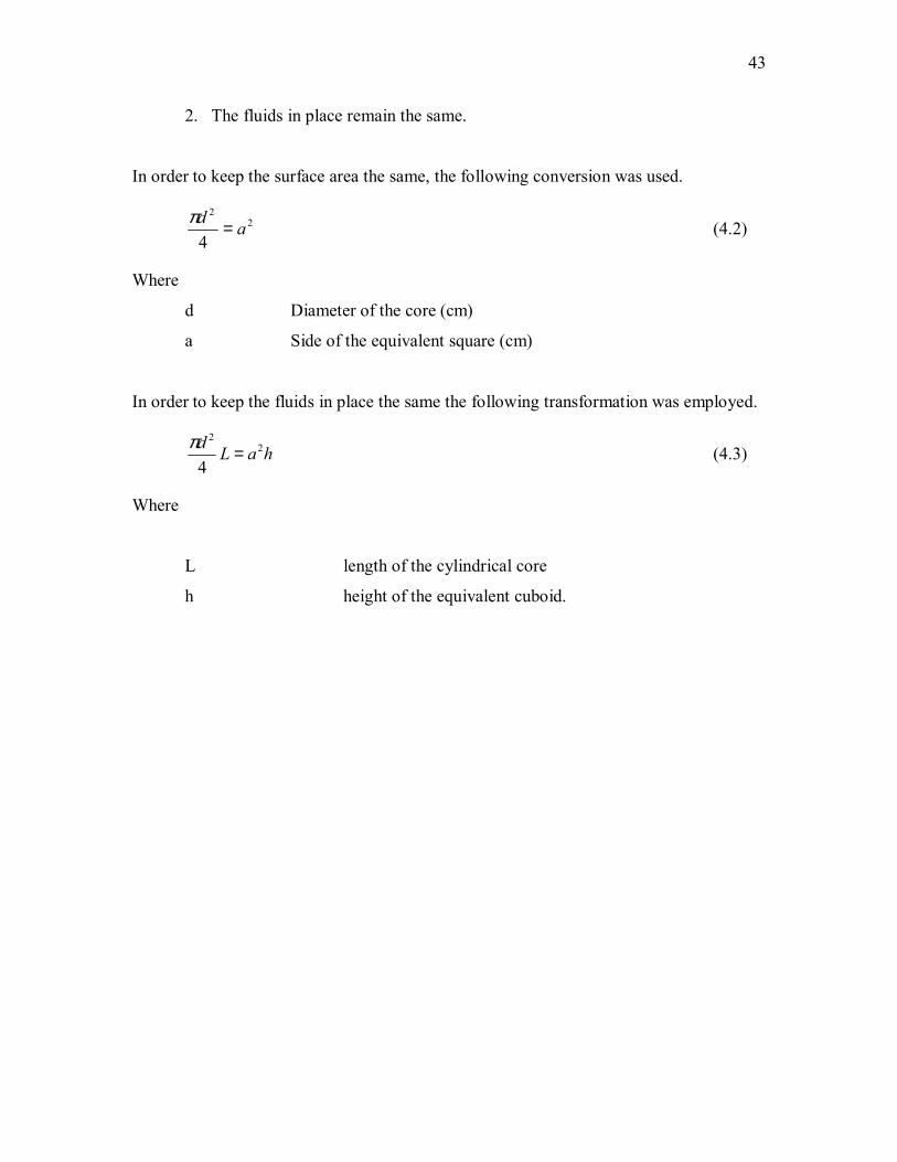
4.1.1.2.1 Change in Shape
The core was modified from cylindrical to cuboid for computational ease. As
shown in Fig. 4.2, the following rules were found to be necessary and sufficient for this
transformation:
1. The surface area to flow remains the same.
43
2. The fluids in place remain the same.
In order to keep the surface area the same, the following conversion was used.
22
4ad =π (4.2)
Where
d Diameter of the core (cm)
a Side of the equivalent square (cm)
In order to keep the fluids in place the same the following transformation was employed.
haLd 22
4=π (4.3)
Where
L length of the cylindrical core
h height of the equivalent cuboid.
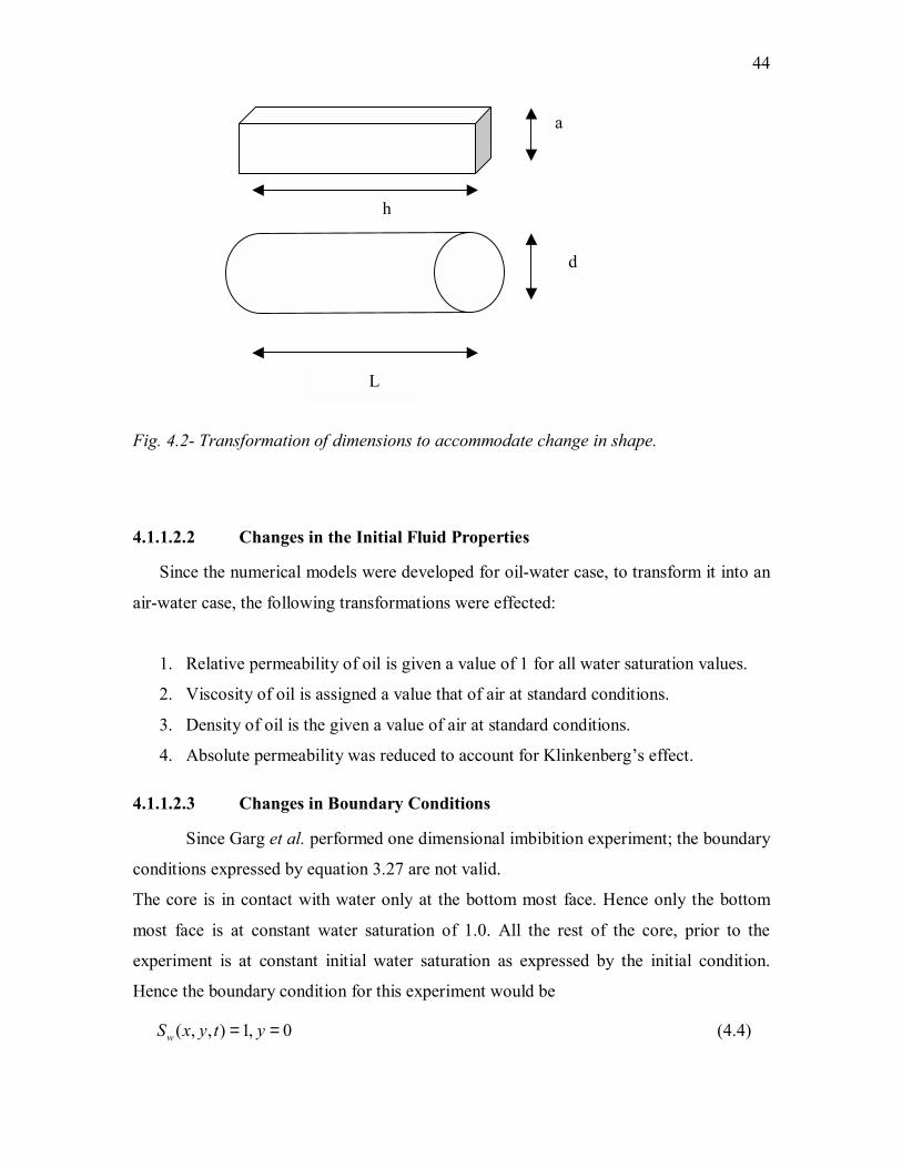
44
Fig. 4.2- Transformation of dimensions to accommodate change in shape.
4.1.1.2.2 Changes in the Initial Fluid Properties
Since the numerical models were developed for oil-water case, to transform it into an
air-water case, the following transformations were effected:
1. Relative permeability of oil is given a value of 1 for all water saturation values.
2. Viscosity of oil is assigned a value that of air at standard conditions.
3. Density of oil is the given a value of air at standard conditions.
4. Absolute permeability was reduced to account for Klinkenberg�s effect.
4.1.1.2.3 Changes in Boundary Conditions
Since Garg et al. performed one dimensional imbibition experiment; the boundary
conditions expressed by equation 3.27 are not valid.
The core is in contact with water only at the bottom most face. Hence only the bottom
most face is at constant water saturation of 1.0. All the rest of the core, prior to the
experiment is at constant initial water saturation as expressed by the initial condition.
Hence the boundary condition for this experiment would be
0,1),,( == ytyxSw (4.4)
L
d
a
h
45
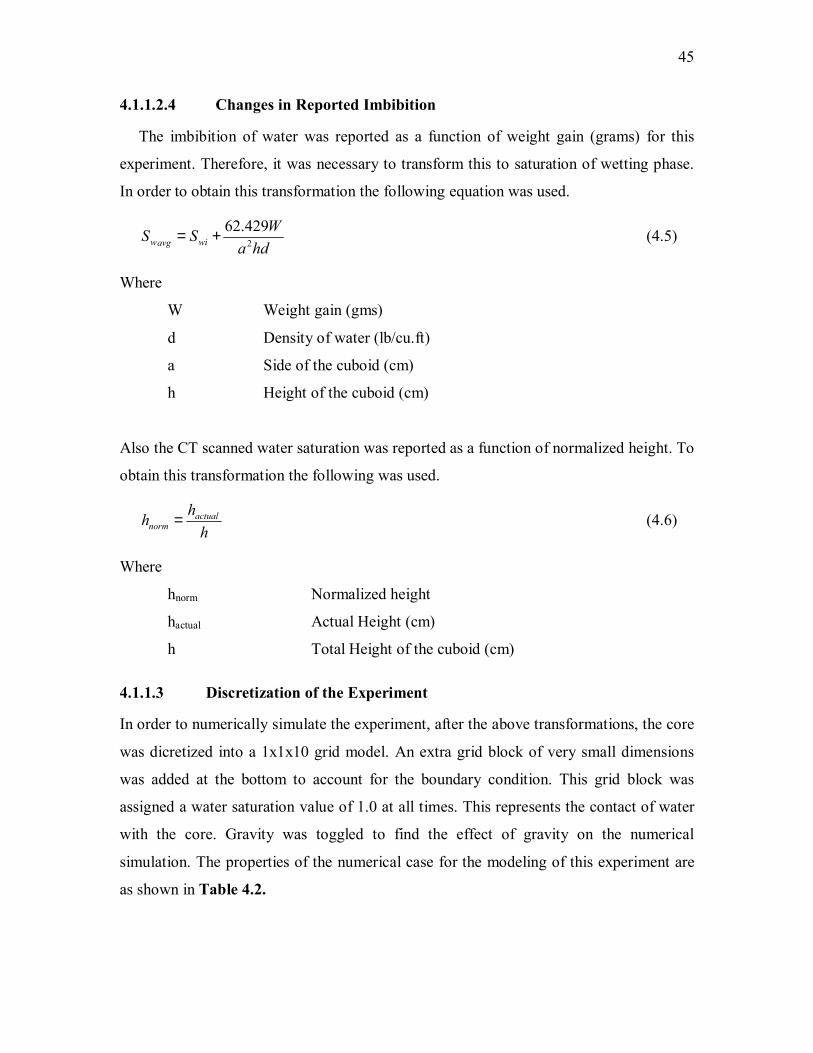
4.1.1.2.4 Changes in Reported Imbibition
The imbibition of water was reported as a function of weight gain (grams) for this
experiment. Therefore, it was necessary to transform this to saturation of wetting phase.
In order to obtain this transformation the following equation was used.
hdaWSS wiavgw 2
429.62+= (4.5)
Where
W Weight gain (gms)
d Density of water (lb/cu.ft)
a Side of the cuboid (cm)
h Height of the cuboid (cm)
Also the CT scanned water saturation was reported as a function of normalized height. To
obtain this transformation the following was used.
hhh actual
norm = (4.6)
Where
hnorm Normalized height
hactual Actual Height (cm)
h Total Height of the cuboid (cm)
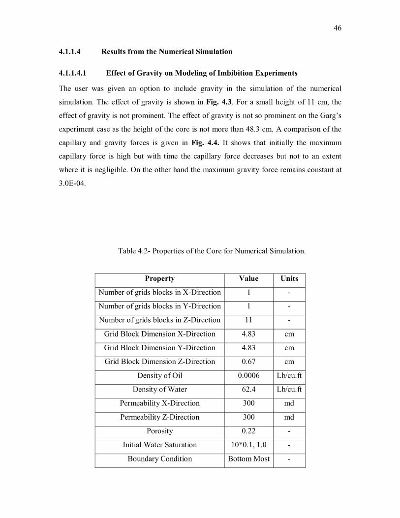
4.1.1.3 Discretization of the Experiment
In order to numerically simulate the experiment, after the above transformations, the core
was dicretized into a 1x1x10 grid model. An extra grid block of very small dimensions
was added at the bottom to account for the boundary condition. This grid block was
assigned a water saturation value of 1.0 at all times. This represents the contact of water
with the core. Gravity was toggled to find the effect of gravity on the numerical
simulation. The properties of the numerical case for the modeling of this experiment are
as shown in Table 4.2.
46
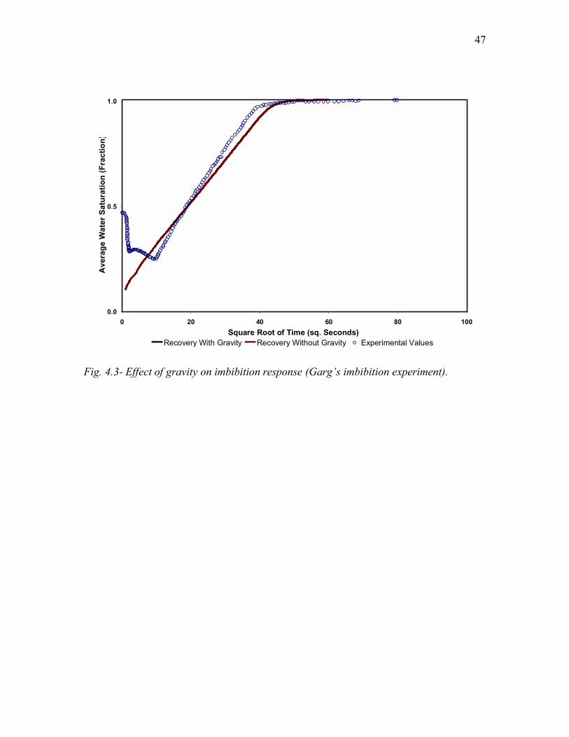
4.1.1.4 Results from the Numerical Simulation
4.1.1.4.1 Effect of Gravity on Modeling of Imbibition Experiments
The user was given an option to include gravity in the simulation of the numerical
simulation. The effect of gravity is shown in Fig. 4.3. For a small height of 11 cm, the
effect of gravity is not prominent. The effect of gravity is not so prominent on the Garg�s
experiment case as the height of the core is not more than 48.3 cm. A comparison of the
capillary and gravity forces is given in Fig. 4.4. It shows that initially the maximum
capillary force is high but with time the capillary force decreases but not to an extent
where it is negligible. On the other hand the maximum gravity force remains constant at
3.0E-04.
Table 4.2- Properties of the Core for Numerical Simulation.
Property Value Units
Number of grids blocks in X-Direction 1 -
Number of grids blocks in Y-Direction 1 -
Number of grids blocks in Z-Direction 11 -
Grid Block Dimension X-Direction 4.83 cm
Grid Block Dimension Y-Direction 4.83 cm
Grid Block Dimension Z-Direction 0.67 cm
Density of Oil 0.0006 Lb/cu.ft
Density of Water 62.4 Lb/cu.ft
Permeability X-Direction 300 md
Permeability Z-Direction 300 md
Porosity 0.22 -
Initial Water Saturation 10*0.1, 1.0 -
Boundary Condition Bottom Most -
47
0.0
0.5
1.0
0 20 40 60 80 100Square Root of Time (sq. Seconds)
Ave
rage
Wat
er S
atur
atio
n (F
ract
ion)
Recovery With Gravity Recovery Without Gravity Experimental Values
Fig. 4.3- Effect of gravity on imbibition response (Garg�s imbibition experiment).
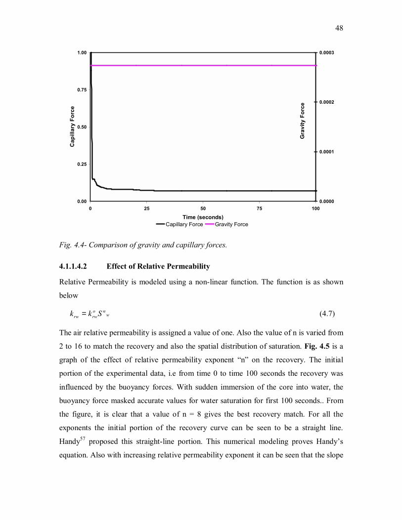
48
0.00
0.25
0.50
0.75
1.00
0 25 50 75 100
Time (seconds)
Cap
illar
y Fo
rce
0.0000
0.0001
0.0002
0.0003
Gra
vity
For
ce
Capillary Force Gravity Force
Fig. 4.4- Comparison of gravity and capillary forces.
4.1.1.4.2 Effect of Relative Permeability
Relative Permeability is modeled using a non-linear function. The function is as shown
below
wno
rwrw Skk = (4.7)
The air relative permeability is assigned a value of one. Also the value of n is varied from
2 to 16 to match the recovery and also the spatial distribution of saturation. Fig. 4.5 is a
graph of the effect of relative permeability exponent �n� on the recovery. The initial
portion of the experimental data, i.e from time 0 to time 100 seconds the recovery was
influenced by the buoyancy forces. With sudden immersion of the core into water, the
buoyancy force masked accurate values for water saturation for first 100 seconds.. From
the figure, it is clear that a value of n = 8 gives the best recovery match. For all the
exponents the initial portion of the recovery curve can be seen to be a straight line.
Handy57 proposed this straight-line portion. This numerical modeling proves Handy�s
equation. Also with increasing relative permeability exponent it can be seen that the slope
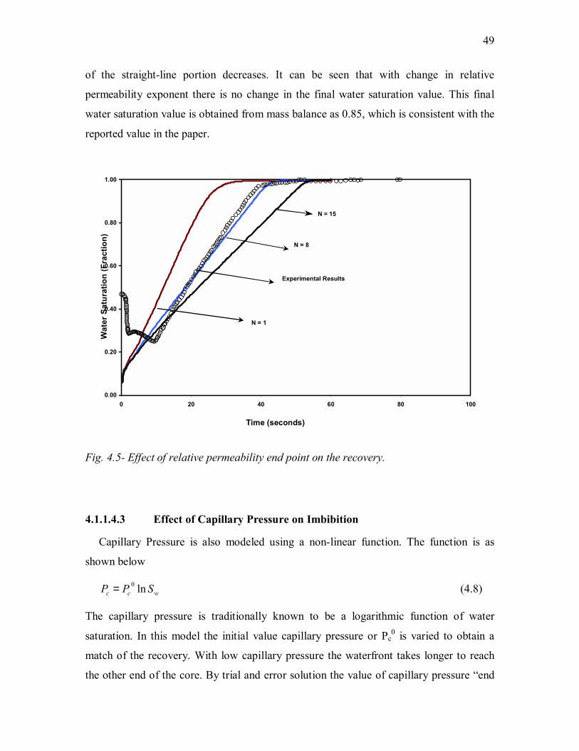
49
of the straight-line portion decreases. It can be seen that with change in relative
permeability exponent there is no change in the final water saturation value. This final
water saturation value is obtained from mass balance as 0.85, which is consistent with the
reported value in the paper.
0.00
0.20
0.40
0.60
0.80
1.00
0 20 40 60 80 100
Time (seconds)
Wat
er S
atur
atio
n (F
ract
ion)
N = 15
N = 8
Experimental Results
N = 1
Fig. 4.5- Effect of relative permeability end point on the recovery.
4.1.1.4.3 Effect of Capillary Pressure on Imbibition
Capillary Pressure is also modeled using a non-linear function. The function is as
shown below
wcc SPP ln0= (4.8)
The capillary pressure is traditionally known to be a logarithmic function of water
saturation. In this model the initial value capillary pressure or Pc0 is varied to obtain a
match of the recovery. With low capillary pressure the waterfront takes longer to reach
the other end of the core. By trial and error solution the value of capillary pressure �end
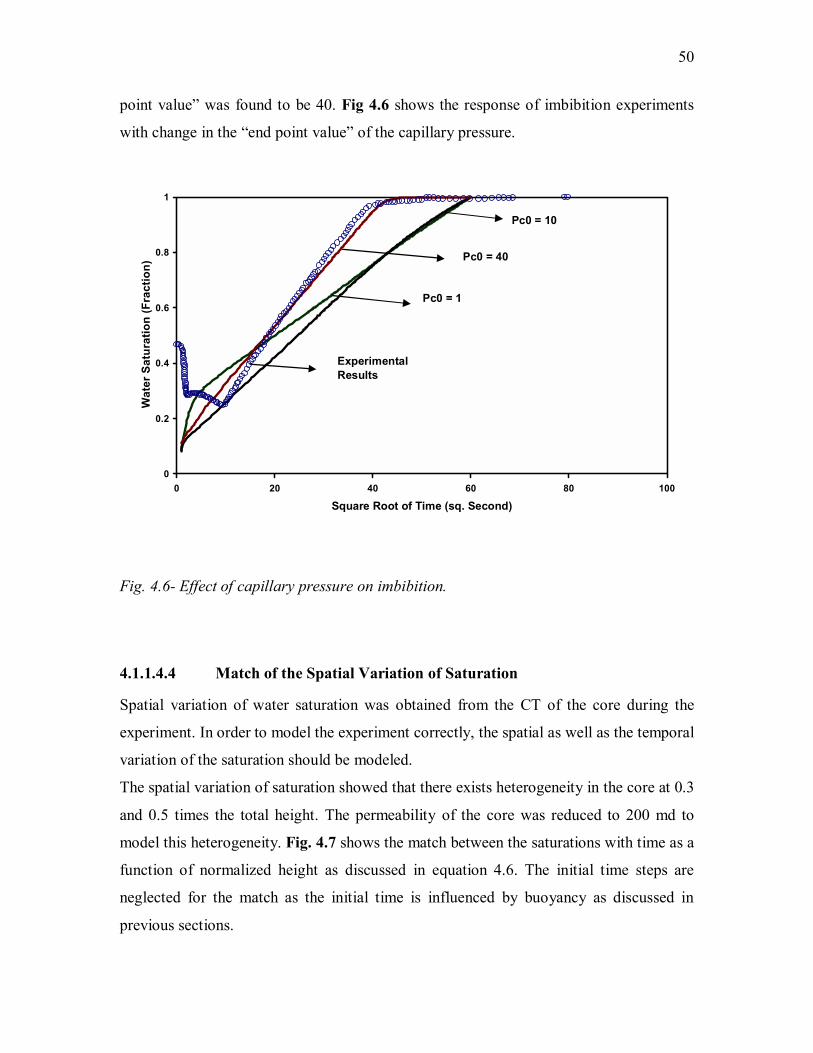
50
point value� was found to be 40. Fig 4.6 shows the response of imbibition experiments
with change in the �end point value� of the capillary pressure.
0
0.2
0.4
0.6
0.8
1
0 20 40 60 80 100
Square Root of Time (sq. Second)
Wat
er S
atur
atio
n (F
ract
ion)
Pc0 = 10
Pc0 = 40
Pc0 = 1
Experimental Results
Fig. 4.6- Effect of capillary pressure on imbibition.
4.1.1.4.4 Match of the Spatial Variation of Saturation
Spatial variation of water saturation was obtained from the CT of the core during the
experiment. In order to model the experiment correctly, the spatial as well as the temporal
variation of the saturation should be modeled.
The spatial variation of saturation showed that there exists heterogeneity in the core at 0.3
and 0.5 times the total height. The permeability of the core was reduced to 200 md to
model this heterogeneity. Fig. 4.7 shows the match between the saturations with time as a
function of normalized height as discussed in equation 4.6. The initial time steps are
neglected for the match as the initial time is influenced by buoyancy as discussed in
previous sections.
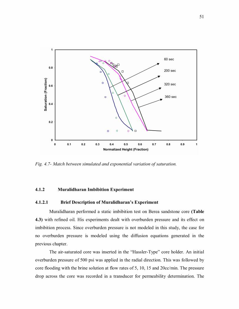
51
0
0.2
0.4
0.6
0.8
1
0 0.1 0.2 0.3 0.4 0.5 0.6 0.7 0.8 0.9 1
Normalized Height (Fraction)
Satu
ratio
n (F
ract
ion)
60 sec
200 sec
320 sec
360 sec
Fig. 4.7- Match between simulated and exponential variation of saturation.
4.1.2 Muralidharan Imbibition Experiment
4.1.2.1 Brief Description of Muralidharan�s Experiment
Muralidharan performed a static imbibition test on Berea sandstone core (Table
4.3) with refined oil. His experiments dealt with overburden pressure and its effect on
imbibition process. Since overburden pressure is not modeled in this study, the case for
no overburden pressure is modeled using the diffusion equations generated in the
previous chapter.
The air-saturated core was inserted in the �Hassler-Type� core holder. An initial
overburden pressure of 500 psi was applied in the radial direction. This was followed by
core flooding with the brine solution at flow rates of 5, 10, 15 and 20cc/min. The pressure
drop across the core was recorded in a transducer for permeability determination. The
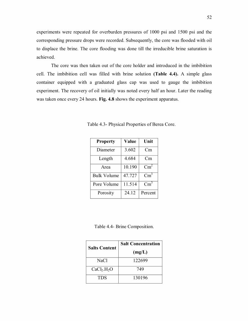
52
experiments were repeated for overburden pressures of 1000 psi and 1500 psi and the
corresponding pressure drops were recorded. Subsequently, the core was flooded with oil
to displace the brine. The core flooding was done till the irreducible brine saturation is
achieved.
The core was then taken out of the core holder and introduced in the imbibition
cell. The imbibition cell was filled with brine solution (Table 4.4). A simple glass
container equipped with a graduated glass cap was used to gauge the imbibition
experiment. The recovery of oil initially was noted every half an hour. Later the reading
was taken once every 24 hours. Fig. 4.8 shows the experiment apparatus.
Table 4.3- Physical Properties of Berea Core.
Property Value Unit
Diameter 3.602 Cm
Length 4.684 Cm
Area 10.190 Cm2
Bulk Volume 47.727 Cm3
Pore Volume 11.514 Cm3
Porosity 24.12 Percent
Table 4.4- Brine Composition.
Salts ContentSalt Concentration
(mg/L)
NaCl 122699
CaCl2.H2O 749
TDS 130196
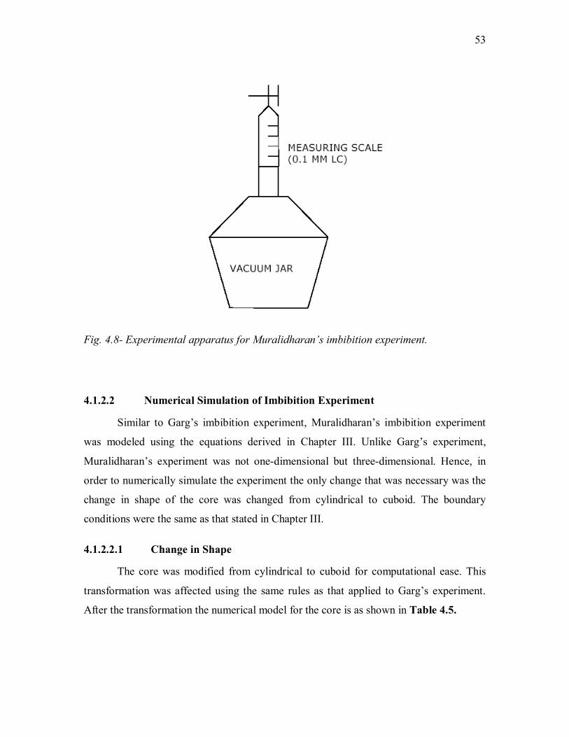
53
Fig. 4.8- Experimental apparatus for Muralidharan�s imbibition experiment.
4.1.2.2 Numerical Simulation of Imbibition Experiment
Similar to Garg�s imbibition experiment, Muralidharan�s imbibition experiment
was modeled using the equations derived in Chapter III. Unlike Garg�s experiment,
Muralidharan�s experiment was not one-dimensional but three-dimensional. Hence, in
order to numerically simulate the experiment the only change that was necessary was the
change in shape of the core was changed from cylindrical to cuboid. The boundary
conditions were the same as that stated in Chapter III.
4.1.2.2.1 Change in Shape
The core was modified from cylindrical to cuboid for computational ease. This
transformation was affected using the same rules as that applied to Garg�s experiment.
After the transformation the numerical model for the core is as shown in Table 4.5.
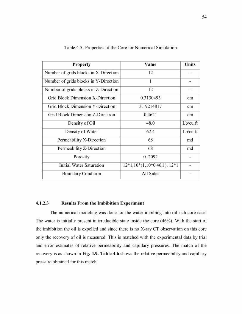
54
Table 4.5- Properties of the Core for Numerical Simulation.
Property Value Units
Number of grids blocks in X-Direction 12 -
Number of grids blocks in Y-Direction 1 -
Number of grids blocks in Z-Direction 12 -
Grid Block Dimension X-Direction 0.3130493 cm
Grid Block Dimension Y-Direction 3.19214817 cm
Grid Block Dimension Z-Direction 0.4621 cm
Density of Oil 48.0 Lb/cu.ft
Density of Water 62.4 Lb/cu.ft
Permeability X-Direction 68 md
Permeability Z-Direction 68 md
Porosity 0. 2092 -
Initial Water Saturation 12*1,10*(1,10*0.46,1), 12*1 -
Boundary Condition All Sides -
4.1.2.3 Results From the Imbibition Experiment
The numerical modeling was done for the water imbibing into oil rich core case.
The water is initially present in irreducible state inside the core (46%). With the start of
the imbibition the oil is expelled and since there is no X-ray CT observation on this core
only the recovery of oil is measured. This is matched with the experimental data by trial
and error estimates of relative permeability and capillary pressures. The match of the
recovery is as shown in Fig. 4.9. Table 4.6 shows the relative permeability and capillary
pressure obtained for this match.
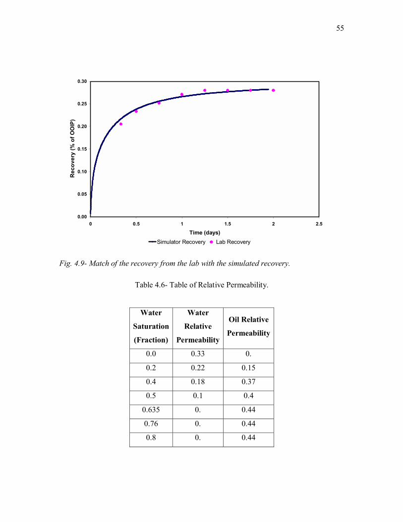
55
0.00
0.05
0.10
0.15
0.20
0.25
0.30
0 0.5 1 1.5 2 2.5
Time (days)
Rec
over
y (%
of O
OIP
)
Simulator Recovery Lab Recovery
Fig. 4.9- Match of the recovery from the lab with the simulated recovery.
Table 4.6- Table of Relative Permeability.
Water
Saturation
(Fraction)
Water
Relative
Permeability
Oil Relative
Permeability
0.0 0.33 0.
0.2 0.22 0.15
0.4 0.18 0.37
0.5 0.1 0.4
0.635 0. 0.44
0.76 0. 0.44
0.8 0. 0.44
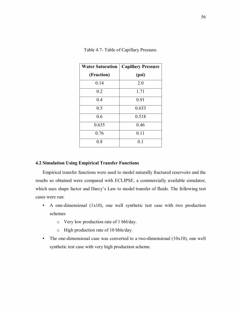
56
Table 4.7- Table of Capillary Pressure.
Water Saturation
(Fraction)
Capillary Pressure
(psi)
0.14 2.0
0.2 1.71
0.4 0.91
0.5 0.653
0.6 0.518
0.635 0.46
0.76 0.11
0.8 0.1
4.2 Simulation Using Empirical Transfer Functions
Empirical transfer functions were used to model naturally fractured reservoirs and the
results so obtained were compared with ECLIPSE, a commercially available simulator,
which uses shape factor and Darcy�s Law to model transfer of fluids. The following test
cases were run:
• A one-dimensional (1x10), one well synthetic test case with two production
schemes
o Very low production rate of 1 bbl/day.
o High production rate of 10 bbls/day.
• The one-dimensional case was converted to a two-dimensional (10x10), one well
synthetic test case with very high production scheme.
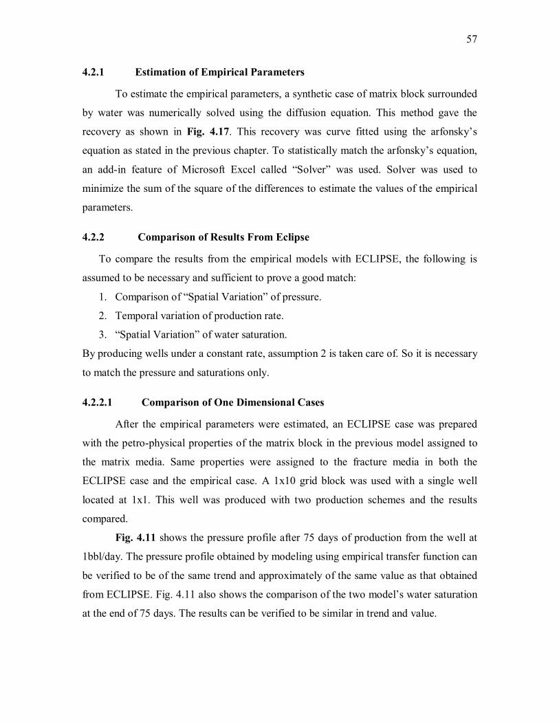
57
4.2.1 Estimation of Empirical Parameters
To estimate the empirical parameters, a synthetic case of matrix block surrounded
by water was numerically solved using the diffusion equation. This method gave the
recovery as shown in Fig. 4.17. This recovery was curve fitted using the arfonsky�s
equation as stated in the previous chapter. To statistically match the arfonsky�s equation,
an add-in feature of Microsoft Excel called �Solver� was used. Solver was used to
minimize the sum of the square of the differences to estimate the values of the empirical
parameters.
4.2.2 Comparison of Results From Eclipse
To compare the results from the empirical models with ECLIPSE, the following is
assumed to be necessary and sufficient to prove a good match:
1. Comparison of �Spatial Variation� of pressure.
2. Temporal variation of production rate.
3. �Spatial Variation� of water saturation.
By producing wells under a constant rate, assumption 2 is taken care of. So it is necessary
to match the pressure and saturations only.
4.2.2.1 Comparison of One Dimensional Cases
After the empirical parameters were estimated, an ECLIPSE case was prepared
with the petro-physical properties of the matrix block in the previous model assigned to
the matrix media. Same properties were assigned to the fracture media in both the
ECLIPSE case and the empirical case. A 1x10 grid block was used with a single well
located at 1x1. This well was produced with two production schemes and the results
compared.
Fig. 4.11 shows the pressure profile after 75 days of production from the well at
1bbl/day. The pressure profile obtained by modeling using empirical transfer function can
be verified to be of the same trend and approximately of the same value as that obtained
from ECLIPSE. Fig. 4.11 also shows the comparison of the two model�s water saturation
at the end of 75 days. The results can be verified to be similar in trend and value.
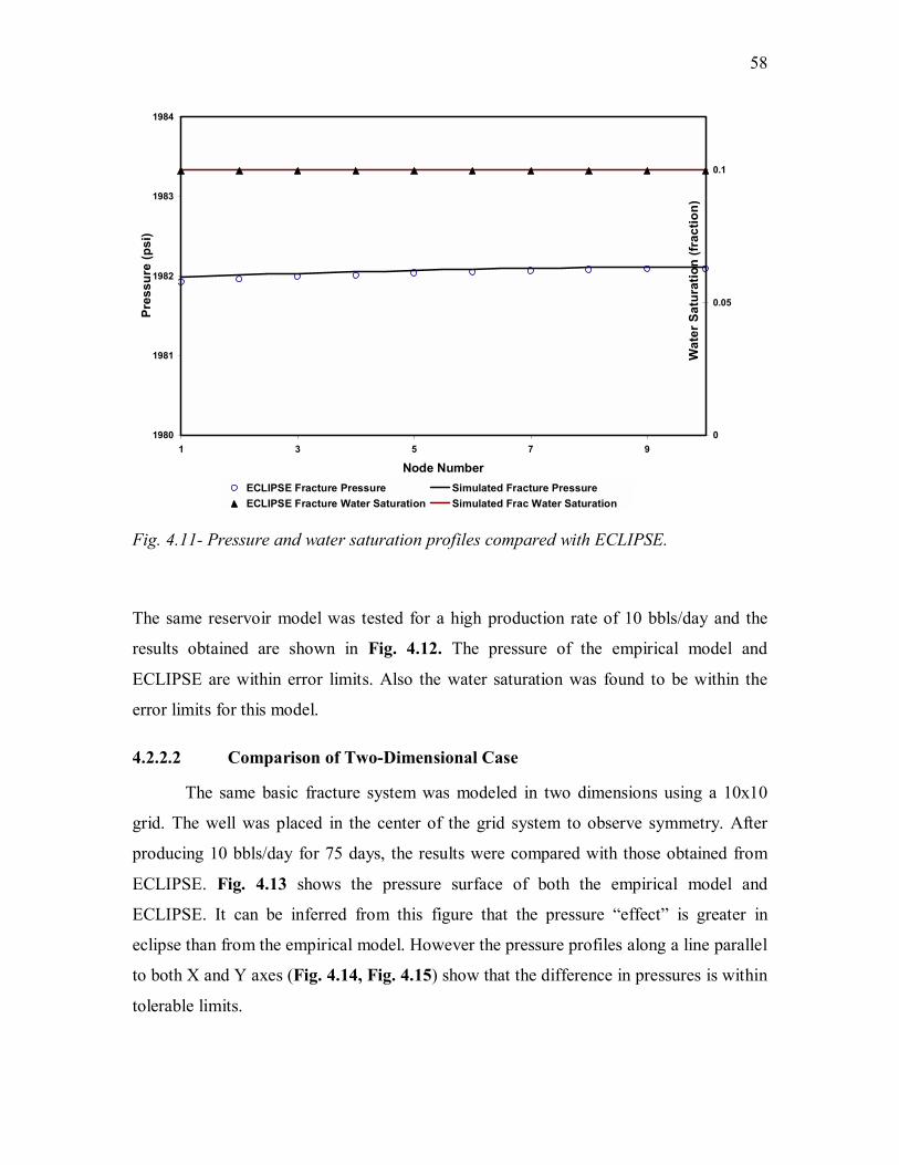
58
1980
1981
1982
1983
1984
1 3 5 7 9
Node Number
Pres
sure
(psi
)
0
0.05
0.1
Wat
er S
atur
atio
n (fr
actio
n)
ECLIPSE Fracture Pressure Simulated Fracture PressureECLIPSE Fracture Water Saturation Simulated Frac Water Saturation
Fig. 4.11- Pressure and water saturation profiles compared with ECLIPSE.
The same reservoir model was tested for a high production rate of 10 bbls/day and the
results obtained are shown in Fig. 4.12. The pressure of the empirical model and
ECLIPSE are within error limits. Also the water saturation was found to be within the
error limits for this model.
4.2.2.2 Comparison of Two-Dimensional Case
The same basic fracture system was modeled in two dimensions using a 10x10
grid. The well was placed in the center of the grid system to observe symmetry. After
producing 10 bbls/day for 75 days, the results were compared with those obtained from
ECLIPSE. Fig. 4.13 shows the pressure surface of both the empirical model and
ECLIPSE. It can be inferred from this figure that the pressure �effect� is greater in
eclipse than from the empirical model. However the pressure profiles along a line parallel
to both X and Y axes (Fig. 4.14, Fig. 4.15) show that the difference in pressures is within
tolerable limits.
59
1800
1810
1820
1830
1840
1 3 5 7 9
Node Number
Pres
sure
(psi
)
0
0.04
0.08
0.12
Wat
er S
atur
atio
n (F
ract
ion)
Fracture Pressure Eclipse Frac Pressure Fracture Saturation Eclipse Saturation Fig. 4.12- Comparison of pressure and water saturation profiles.
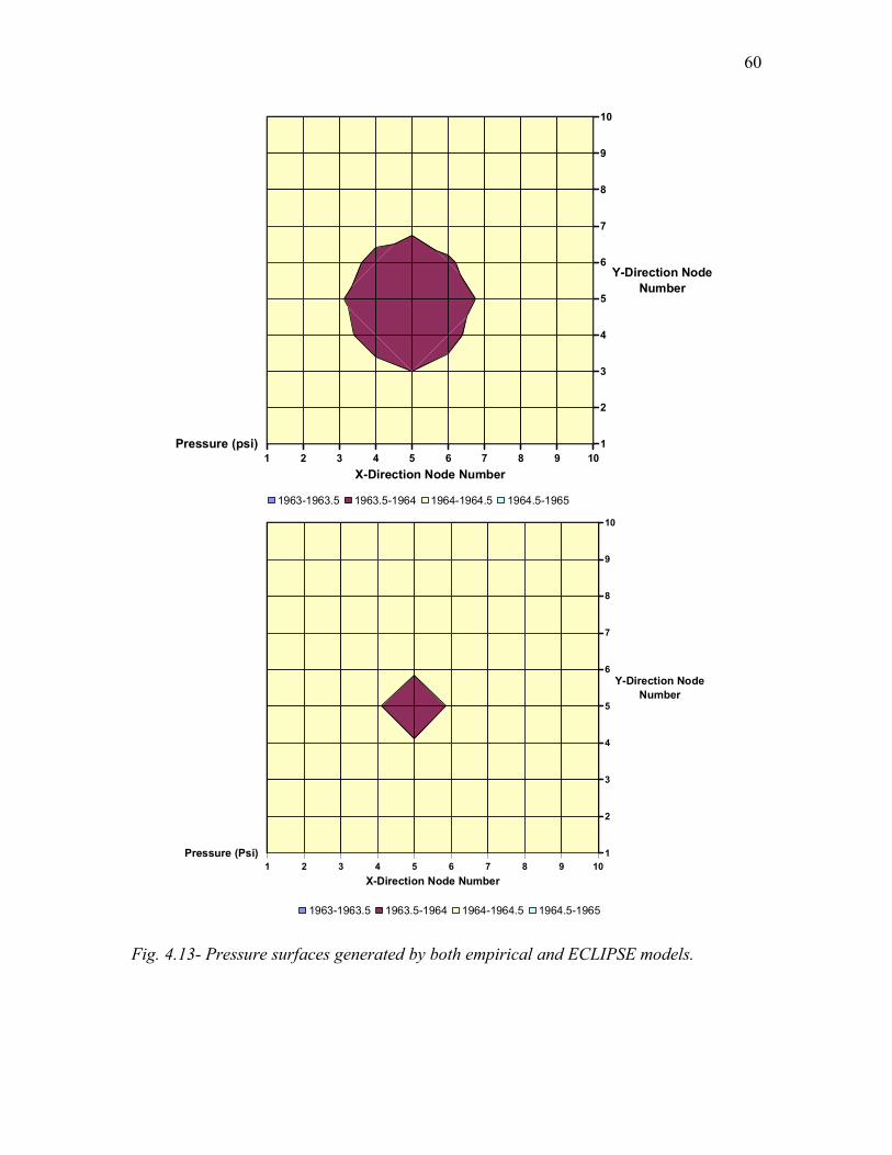
60
1 2 3 4 5 6 7 8 9 101
2
3
4
5
6
7
8
9
10
Pressure (psi)
X-Direction Node Number
Y-Direction Node Number
1963-1963.5 1963.5-1964 1964-1964.5 1964.5-1965
1 2 3 4 5 6 7 8 9 101
2
3
4
5
6
7
8
9
10
Pressure (Psi)
X-Direction Node Number
Y-Direction Node Number
1963-1963.5 1963.5-1964 1964-1964.5 1964.5-1965
Fig. 4.13- Pressure surfaces generated by both empirical and ECLIPSE models.
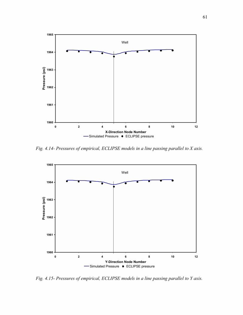
61
1960
1961
1962
1963
1964
1965
0 2 4 6 8 10 12
X-Direction Node Number
Pres
sure
(psi
)
Simulated Pressure ECLIPSE pressure
Well
Fig. 4.14- Pressures of empirical, ECLIPSE models in a line passing parallel to X axis.
1960
1961
1962
1963
1964
1965
0 2 4 6 8 10 12
Y-Direction Node Number
Pres
sure
(psi
)
Simulated Pressure ECLIPSE pressure
Well
Fig. 4.15- Pressures of empirical, ECLIPSE models in a line passing parallel to Y axis.

62
Both Fig. 4.14 and 4.15 are identical. This is because of the symmetry of the model. This
identicalness is necessary for the formulation to be correct.
Fig. 4.17 shows the saturation surface generated by both the empirical and
ECLIPSE models. It can be seen that the saturation difference is more significant than the
pressure difference. This can be attributed to the difference in formulation of transfer of
fluids from the matrix to the fracture.
0
0.25
0.5
0.75
1
0 15 30 45 60
Time (days)
Rec
over
y
Results from Simulation Curve Fitting
Curve Fitting ParametersRinf = 1.0lamda = 0.031
Fig. 4.16- Curve fitting recovery with exponential decline equation.
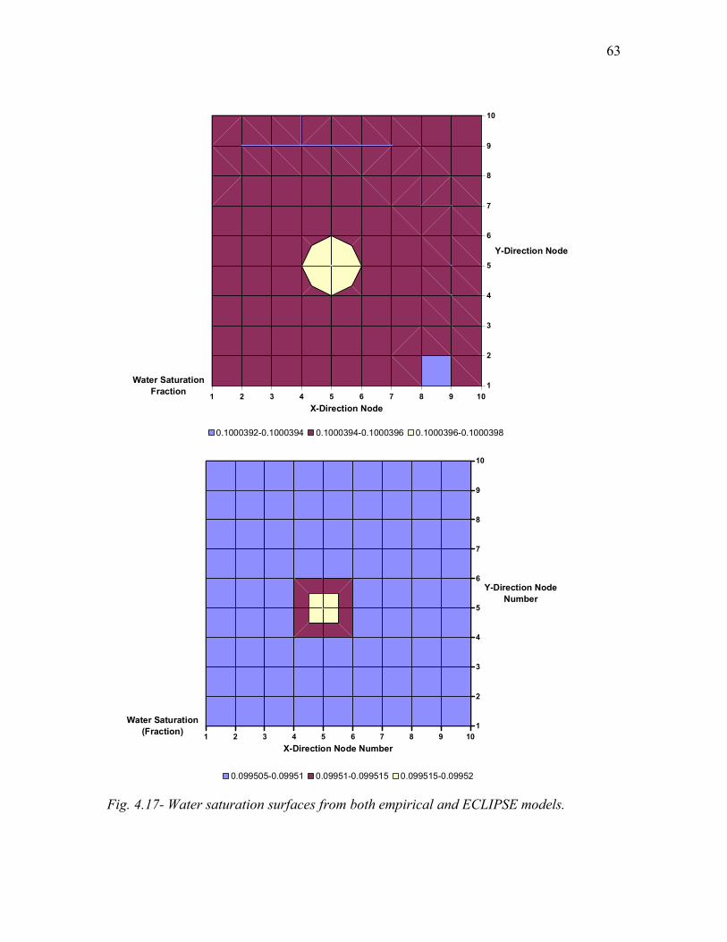
63
1 2 3 4 5 6 7 8 9 101
2
3
4
5
6
7
8
9
10
Water Saturation Fraction
X-Direction Node
Y-Direction Node
0.1000392-0.1000394 0.1000394-0.1000396 0.1000396-0.1000398
1 2 3 4 5 6 7 8 9 101
2
3
4
5
6
7
8
9
10
Water Saturation (Fraction)
X-Direction Node Number
Y-Direction Node Number
0.099505-0.09951 0.09951-0.099515 0.099515-0.09952 Fig. 4.17- Water saturation surfaces from both empirical and ECLIPSE models.
64
4.2.3 Comparison with Sub-Domain Method
Kazemi and Gilman26 presented a 5 spot synthetic water flooding case. From this
case, a grid block was selected and synthetic imbibition experiments were performed.
The matrix was initially filled with recoverable oil and completely surrounded by
fractures. The fracture spacing was selected in such a manner that the matrix block is of
the same size as that of the grid block. Fractures that surround the matrix block were
saturated with water and a field size imbibition experiment was thus created. A graphical
representation of this model is shown in Fig. 4.18.
This model was simulated using a commercially available simulator CMG and
also by the developed empirical transfer function dual porosity simulator. Fig. 4.19
shows the matrix saturation results from the commercially available simulator and the
developed simulator. �Sub-Domain� method, which is a refinement of dual porosity
simulation, was also used for this test case. Sub-domain method reports the matrix
saturation slightly less than that of the conventional dual porosity simulation. This is
because of matrix block refinement in case of sub-domain method. In this test case, a 5
level sub-domain method was used, that is, matrix was divided into five different blocks
and the average saturation of these divisions were reported as the matrix saturation.
The empirical transfer function model compares well with both these models. In the
initial portion of Fig. 4.19, it can be seen that the empirical transfer function�s results are
within error of sub-domain method while offset from the conventional dual porosity
results. This is because the conventional transfer functions formulations do not honor the
initial time behavior of transfer of fluids56. The later time behavior of empirical transfer
function model is within acceptable limits of both conventional transfer function model
and sub-domain models.

65
Fig. 4.18- Grid block39 modeled using empirical and sub-domain methods.
0
0.2
0.4
0.6
0.8
1
0 1000 2000 3000 4000
Time (Days)
Mat
rix W
ater
Sat
urat
ion
(Fra
ctio
n)
SubDomain Dual Poro Using 10 Grid Blocks Using 15 gridBlock Fig. 4.19- Comparison of ETF with sub-domain method and conventional methods.
66
4.2.4 Limitations of Empirical Transfer Function
In its present formulation, the empirical transfer function can be used for
simulation of two phase (oil-water) fluid flow. In order to extend this theory to cases
where gas is also present, compressibility of gas, which is also a driving force needs to be
considered. Similarly three phase flow cannot be simulated using this transfer function.
Another limitation of this theory is the limited �time step ability�, that is present
with this case. The integration is equation 3.71 is computed numerically using a
summation term as shown in equations 3.72 and 3.73. This assumption that an integral
can be accurately represented by a summation is valid only when the time steps are small.
Hence very large time steps can lead to inaccurate results. A comparison of the material
balance error obtained when using large steps is shown in Fig. 4.20. As can be seen from
this graph, the oil material balance for the two dimensional case presented earlier,
increases linearly with time.
Since this theory is based on Aronofsky�s equation, all the assumptions inherent
in Aronofsky�s equation can also be extended to this theory.
4.2.5 Correlation to Well-Test Parameters
Dual porosity systems need two additional parameters for characterization than
the homogeneous and isotropic reservoirs. These are called the interporosity flow
coefficient and the storativity ratio usually denoted by λ and ω respectively. The
storativity ratio is a measure of the fluid stored in the fracture system compared to the
total fluid in the reservoir. The interporosity flow coefficient determines the inter-relation
between matrix and fracture continua.

67
-1.E-02
-8.E-03
-6.E-03
-4.E-03
-2.E-03
0.E+000 10 20 30 40 50 60 70 80
Time (days)
Oil
Mat
eria
l Bal
ance
Err
or (p
erce
nt)
-2.E-04
-1.E-04
-8.E-05
-4.E-05
0.E+00
4.E-05
Wat
er M
ater
ial B
alan
ce E
rror
(Per
cent
)
Oil Phase Water Phase
Fig. 4.20- Material balance error when using large time steps (10 days).
These two parameters, λ and ω, are usually calculated from pressure transient
analysis. Their relations to the reservoir parameters are given by:
2w
m rk
kαλ = (4.9)
( )
( ) ( )mtft
ft
ccc
φφφ
ω+
= (4.10)
α is a geometric factor that depends on the shape of the matrix blocks and has dimensions
of lenght-2. The subscripts m and f refer to matrix and fracture systems respectively.
Higher interporosity flow coefficients indicate ease of transfer of fluids from the
matrix to the fracture continua. This means that it takes lesser time for fluids to move
from matrix to fracture. Recalling Aronofsky�s equation, the time taken to reach the
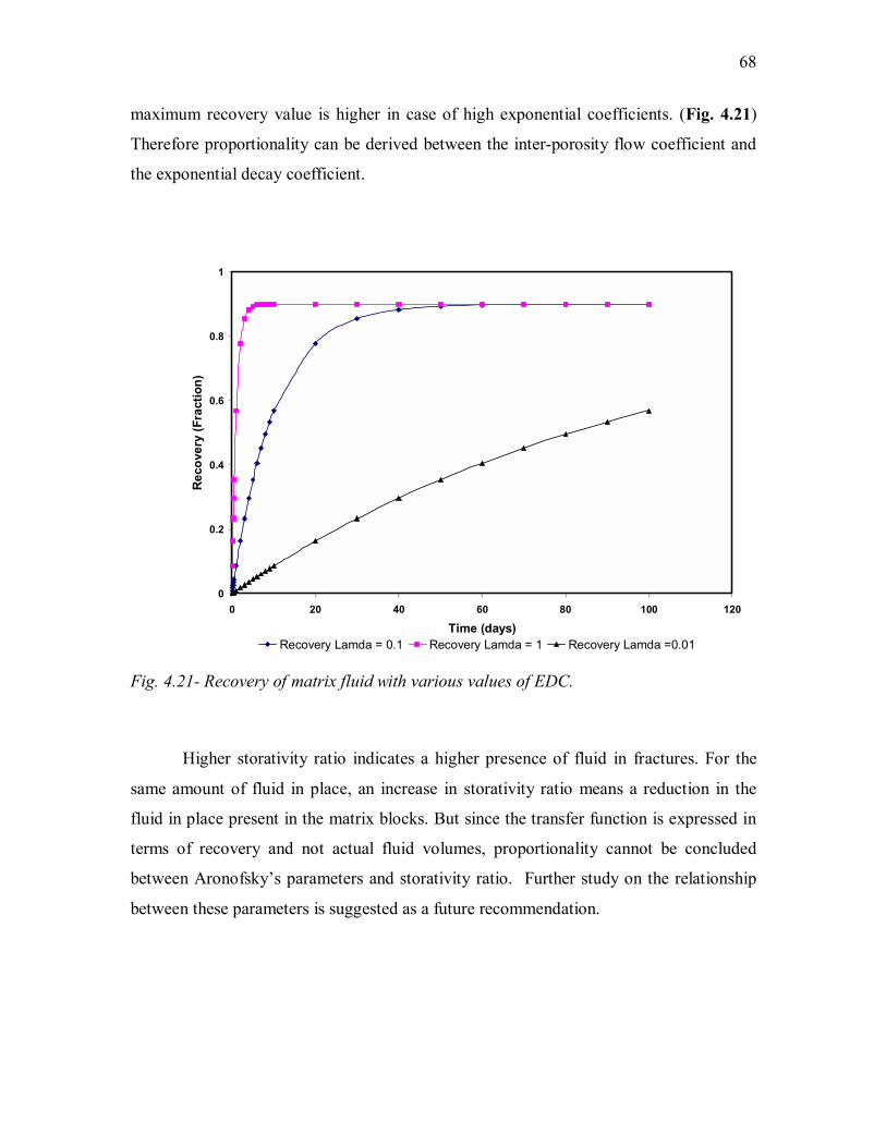
68
maximum recovery value is higher in case of high exponential coefficients. (Fig. 4.21)
Therefore proportionality can be derived between the inter-porosity flow coefficient and
the exponential decay coefficient.
0
0.2
0.4
0.6
0.8
1
0 20 40 60 80 100 120
Time (days)
Reco
very
(Fra
ctio
n)
Recovery Lamda = 0.1 Recovery Lamda = 1 Recovery Lamda =0.01
Fig. 4.21- Recovery of matrix fluid with various values of EDC.
Higher storativity ratio indicates a higher presence of fluid in fractures. For the
same amount of fluid in place, an increase in storativity ratio means a reduction in the
fluid in place present in the matrix blocks. But since the transfer function is expressed in
terms of recovery and not actual fluid volumes, proportionality cannot be concluded
between Aronofsky�s parameters and storativity ratio. Further study on the relationship
between these parameters is suggested as a future recommendation.
69
5
CHAPTER V
CONCLUSIONS
The following conclusions can be derived from this study:
• Diffusivity equation is sufficient to model imbibition experiments.
• Imbibition experiments provide us with empirical transfer functions that can be
used to model dual porosity simulation.
• Empirical dual porosity simulation is inherently faster, since the number of
unknowns per grid block is reduced to two from four.
• Empirical transfer functions model transient flow of fluids from matrix to
fractures.
• Synthetic imbibition experiments can be created and modeled using diffusivity
equation. Thus there is no necessity of imbibition experiments for this dual
porosity formulation.
• History matching can be done by �tweaking� only one empirical transfer function
parameter.

70
NOMENCLATURE
a = Side of a cuboid, cm
br= Right hand side matrix
ct = CT number
d = Diffusivity coefficient
e = Exponential constant, 2.7182
g = Acceleration of gravity, ft/sec2
h = Height of core, cm
h = Formation thickness , ft
k = Absolute permeability, md
kro = Relative permeability to oil, dimensionless
krw = Relative permeability to water, dimensionless
krwo = End-point of the relative permeability to water, dimensionless
n = Exponent of the relative permeability to water, dimensionless
Nma= Number of matrix blocks
L = Fracture spacing, ft
Lf = Fracture length, ft
q = Inter-porosity flow rate, rb/day
Q = Flow rate, STB/D
p = Pressure, psia
Pc = Capillary pressure, psia
R = Recovery of oil from matrix, dimensionless
Rr
= Residual matrix
S = Saturation of phase, fraction
t = Time, days
tD = Dimensionless time
VR = Bulk volume, ft3
VP = Pore volume, ft3
xr = Matrix of unknowns in residual form

71
Xr
= Matrix of unknowns in conventional form
α = Coefficients for Gaussian elimination method
β = Residuals in Gaussian elimination method.
wλ = Mobility of water, md/cp
oλ = Mobility of oil, md/cp
Tλ = Total Mobility, md/cp
λ = Exponential decline exponent
3,2,1λ = Civan�s exponential decline constant
ur = Flow rate, rb/ft2-day
τ = Inter-porosity flow rate, ft3/day
φ = Porosity, fraction
µ = Viscosity, cp
ρ = Density, lb/ft3
Φ = Flow potential, psia
σ = Shape factor, ft-2
Subscripts
D = Dimensionless
f = Fracture
i = Initial value
m = Matrix
o = Oil phase
w = Water phase
x = x-direction
y = y-direction
z = z-direction
avg = Average
water = Value of water
dry = Value of dry sample
72
REFERENCES
1. Nelson R.: Geological Analysis of Naturally Fractured Reservoirs, second
edition, Gulf Professional Publishing, St. Louis (2003).
2. Jaeger, J.S. and Cook, N.G.W.: Fundamentals of Rock Mechanics, third edition,
Chapman and Hall Ltd., New York City (1979).
3. Aguilera, R.: Naturally Fractured Reservoirs, second edition, PennWell Pub. Co.,
Tulsa (1995).
4. Reiss, L.H.: The Reservoir Engineering Aspects of Fractured Reservoirs, Gulf
Pub. Co., Houston (1980).
5. van Golf-Racht, T.D.: Fundamentals of Fractured Reservoir Engineering,
Elsevier Scientific Pub. Co., Amsterdam (1982).
6. Nelson, R.A.: Geologic Analysis of Naturally Fractured Reservoirs, Gulf Pub.
Co., Houston (1985).
7. Rock Fractures and Fluid Flow: Contemporary Understanding and Applications,
Committee on Fracture Characterization and Fluid Flow, National Academy
Press, Washington, D.C. (1996).
8. Livak, B.L.: �Simulation and Characterization of Naturally Fractured Reservoirs,�
paper presented at the 1985 Reservoir Characterization Technical Conference,
Dallas.
9. Gilman, J.R. and Kazemi, H.: �Improved Calculations for Viscous and Gravity
Displacement in Matrix Blocks in Dual-Porosity Simulators,� JPT (January 1988)
60-70.
10. Labastie, A.: �Capillary Continuity between Blocks of a Fractured Reservoir,�
paper SPE 20515 presented at the 1990 SPE Annual Technical Conference and
Exhibition, New Orleans, September 23-26.
11. Tan, J.C.T. and Firoozabadi, A.: �Dual-Porosity Simulation Incorporating
Reinfiltration and Capillary Continuity Concepts: Part I � Single Gridcell,� paper
SPE 29113 presented at the 1995 SPE Reservoir Simulation Symposium, San
Antonio, February 12-15.
73
12. Firoozabadi, A. and Ishimoto, K: �Theory of Reinfiltration in Fractured Porous
Media: Part I � One-Dimensional Model,� paper SPE 21796 presented at the 1991
Western Regional Meeting, Long Beach, California, March 20-22.
13. Barkve, T. and Firoozabadi, A.: �Analysis of Reinfiltration in Fractured Porous
Media,� paper SPE 24900 presented at the 1992 Annual Technical Conference
and Exhibition, Washington, D.C., October 4-7.
14. Bourbiaux, B. and Kalaydjian, F.J.: �Experimental Study of Cocurrent and
Countercurrent Flows in Natural Porous Media,� SPERE (August 1990) 361-368.
15. Pooladi-Darvish, M. and Firoozabadi, A.: �Cocurrent and Countercurrent
Imbibition in a Water-Wet Matrix Block,� SPEJ (March 2000) 3-11.
16. McNaughton, D.A., and F.A. Garb. �Finding and Evaluating Petroleum
Accumulations in Fractured Reservoir Rock.� Exploration and Economics of the
Petroleum Industry, (1975) 13, 45-54.
17. Hohlt, R.B. �The Nature of Origin of Limestone Porosity�, Colorado School of
Mines Quarterly (1948) 4, 5-51.
18. Lawn, B. and Wilshaw, R. �Indentation Fracture: Principles and Applications�, J.
Mater. Sci. (UK) (June 1975) 10, 1049-81.
19. Agarwal, B., Hermansen, H., Sylte, J.E., and Thomas, L.K.: �Reservoir
Characterization of Ekofisk Field: A Giant, Fractured Chalk Reservoir in the
Norwegian North Sea � History Match,� SPEREE (December 2000), 534-543.
20. Barenblatt, G.I., Zheltov, I.P., and Kochina, I.N.: �Basic Concepts in the Theory
of Seepage of Homogenous Liquids in Fissured Rocks (Strata),� J. Appl. Math.
Mech. (1960) 24, 1286-1303.
21. Warren, J.E. and Root, P.J.: �The Behavior of Naturally Fractured Reservoirs,�
SPEJ (September 1963) 245-255.
22. Kazemi, H.: �Pressure Transient Analysis of Naturally Fractured Reservoirs with
Uniform Fracture Distribution,� SPEJ (December 1969) 451-462; Trans., AIME,
246.
23. Abdassah, D. and Ershaghi, I.: �Triple-Porosity Systems for Representing
Naturally Fractured Reservoirs,� SPEFE (April 1986) 113-127.
74
24. Aronofsky, J.S., Masse, L., and Natanson, S.G.: �A Model for the Mechanism of
Oil Recovery from the Porous Matrix Due to Water Invasion in Fractured
Reservoirs,� Trans., AIME (1958) 213, 17-19.
25. de Swaan, A.: �A Theory of Waterflooding in Fractured Reservoirs,� SPEJ (April
1978) 117-122; Trans., AIME, 265.
26. Kazemi, H., Gilman, J.R., and Elsharkawy, A.M.: �Analytical and Numerical
Solution of Oil Recovery From Fractured Reservoirs With Empirical Transfer
Functions,� SPERE (May 1992) 219-227.
27. Ries J. and Cil M.: �Analytical Model for Capillary Imbibition: Multidimensional
Matrix Blocks,� In Situ, (2000) 24, No. 1, 79-106.
28. Civan, F.: �Waterflooding of Naturally Fractured Reservoirs: An Efficient
Simulation Approach,� paper SPE 25449 presented at the 1993 Production
Operations Symposium, Oklahoma City, March 21-23.
29. Gupta, A. and Civan, F.: �An Improved Model for Laboratory Measurement of
Matrix to Fracture Transfer Function Parameters in Immiscible Displacement,�
paper SPE 28929 presented at the 1994 SPE Annual Technical Conference and
Exhibition, New Orleans, September 25-28.
30. Civan, F.: �Quadrature Solution for Waterflooding of Naturally Fractured
Reservoirs,� SPEREE (April 1998) 141-147.
31. Rapoport, L.A.: �Scaling Laws for Use in Design and Operation of Water/Oil
Flow Models,� Trans., AIME (1955) 204, 143.
32. Mattax, C.C. and Kyte, J.R.: �Imbibition Oil Recovery from Fractured, Water-
Drive Reservoirs,� SPEJ (June 1962) 177-184.
33. Du Prey, E. L.: �Gravity and Capillary Effects on Imbibition in Porous Media�
Soc. Pet. Eng. J. (June 1978) 195-206.
34. Ma, S., X. Zhang, and N.R. Morrow: �Influence of Fluid Viscosity on Mass,
Transfer Between Rock Matrix and Fractures,� paper presented at the 1995
Annual Technical Meeting of the Petroleum Society of CIM in Banff, Alberta,
Canada, May 14-17.
35. Bourbiaux, B. and Kalaydjian, F.J.: �Experimental Study of Cocurrent and
Countercurrent Flows in Natural Porous Media,� SPERE (August 1990) 361-368.
75
36. Peñuela-Pineda, G.: �Modeling Interporosity Flow for Improved Simulation of
Naturally Fractured Reservoirs,� Ph.D. dissertation (2002), University of
Oklahoma, Norman.
37. Thomas, L.K., Dixon, T.N., and Pierson, R.G.: �Fractured Reservoir Simulation,�
SPEJ (February 1983) 42-54.
38. Coats, K.H.: �Implicit Compositional Simulation of Single-Porosity and Dual-
Porosity Reservoirs,� paper SPE 18427 presented at the 1989 SPE Reservoir
Simulation Symposium, Houston, February 6-8.
39. Gilman, J.R. and Kazemi, H.: �Improvements in Simulation of Naturally
Fractured Reservoirs,� SPEJ (August 1983) 695-707.
40. Lim, K.T. and Aziz, K.: �Matrix-Fracture Transfer Shape Factors for Dual-
Porosity Simulators,� J. Pet. Sci. and Eng. (1995) 13, 169-178.
41. Quintard, M. and Whitaker, S.: �Transport in Chemically and Mechanically
Heterogeneous Porous Media,� Adv. in Water Res., (1996) 19, No. 1, 29-60.
42. Noetinger, B. and Estebenet, T.: �Application of Random Walk Methods on
Unstructured Grid to Up-Scale Fractured Reservoirs,� paper presented at the 1998
European Conference on Mathematics of Oil Recovery, Peebles, Scotland,
September 8-11.
43. Chen, J., M,A, Miller, and K. Sepehrnoori: �Theoretical Investigation of
Countercument Imbibition in Fractured Reservoir Matrix Blocks,� paper SPE
29141 presented at 1995 SPE Symposium on Reservoir Simulation, San Antonio,
Texas, February 12-15.
44. Hernandez J.C. and C.P. Resales: �Imbibition as a Dispersion Process,� paper
SPE 23748 presented at the 1992 SPE Latin American Petroleum Engineering
Conference, Caracas, Venezuela, March 8-11.
45. Hayashi, J.A. and C.P. Resales: �Visual Investigation of Imbibition Process,�,
paper SPE 23745 presented at the 1992 SPE Latin American Petroleum
Engineering Conference, Caracas, Venezuela, March 8-11.
46. Najurieta, H.L.: �A Theory for Pressure Transient Analysis in Naturally Fractured
Reservoirs,� JPT (July 1980) 1241-1250.
76
47. Siddiqui, S., Hicks, P.J., Grader, A.S: �Verification of Buckley-Leverett Three
Phase Theory Using Computerized Tomography�, J. Pet. Sci. and Engg. (1996)
15, 1-21.
48. Houndsfield, G.N: �A Method of and Apparatus for Examining a Body by
Radiation Such as X- or Gamma-Radiation,� Br. Patent No. 1,283,915.
49. Hunt, P.K., Engler, P. and Bajsarowicz, C.: �Computerized Tomography as a
Core Analysis Tool: Applications, Instrument Evaluation and Image Improvement
Techniques�, Soc. Pet. Eng. J., Formation Evaluation (September 1988) 1203-
1210.
50. Hicks, P.J., Deans, H.A., and Narayanan, K.: �Experimental Measurement of the
Distribution of the Residual Oil Saturations in Heterogeneous Carbonate Cores
Using X-ray Computerized Tomography,�, paper CIM/SPE 9068 presented at the
1990 International Technical Meeting, Calgary, Alberta, June 10-13.
51. Peters, E.J. and Afzal, N.: �Characterization of Heterogeneities in Permeable
Media with Computerized Tomography,� Soc. Pet. Eng. J. (1990) 7: 283-296.
52. Moss, R.M. et al.: �Direct Measurement of the Constituent Properties in a Dual
Porosity Matrix,� presented at the 1990 SCA Ann. Tech. Conf., Houston, August
2-3.
53. Aziz, K. and Settari, A.: Petroleum Reservoir Simulation, first edition, Applied
Science Publishers, London, UK (1983).
54. Toronyi, R. M. and Forouq Ali, S. M.: � Determining Interblock Transmissibility
in Reservoir Simulators,� JPT (1979), 26, No. 1, pp. 77-78.
55. Raithby, G. D.: �A Critical Evaluation of Upstream Differencing Applied to
Problems Involving Fluid Flow,� Comp. Methd. in Appl. Mech. and Engg., 9,
No.1, 75-103.
56. Aziz, K. and Lim, K.T.: �Matrix-Fracture Transfer Shape Factors for Dual
Porosity Simualtors,� J. Pet. Sci. and Engg. (1995) 13, 169-178.
57. Handy, L.L.: �Determination of Effective Capillary Pressures for Porous Media
from Imbibition Data,� SPEJ Petroleum Transactions, AIME, (1960) 219, 75-80.
58. Garg, A., Zwahlen, E. and Patzek, T.W.: �Experimental and Numerical Studies of
One-Dimensional Imbibition in Berea Sandstone,� paper presented at the 16th

77
Annual American Geophysical Union Hydrology Days, Fort Collins, Colorado,
April, 15-18.
59. Muralidharan, V., Putra, E., and Schechter, D.S.: �Investigating the Changes in
Matrix and Fracture Properties and Fluid Flow Under Different Stress-State
Conditions,� SA Journal of Technology, Fall 2004.
78
VITA
The author, Prasanna K. Tellapaneni was born in Hyderabad, India. He attended the
Indian School of Mines from 1996 to 2000 and received a Bachelor of Technology in
petroleum engineering in 2000. He began work toward a Master of Science in petroleum
engineering at the Texas A&M University at College Station in the Fall of 2001. The
address of the author is
Mr. Prasanna K. Tellapaneni,
C/O, Dr. Schechter,
3119, Texas A&M University,
College Station, TX 77840.