Embed Size (px)
Citation preview

HAL Id: tel-02447641https://tel.archives-ouvertes.fr/tel-02447641
Submitted on 21 Jan 2020
HAL is a multi-disciplinary open accessarchive for the deposit and dissemination of sci-entific research documents, whether they are pub-lished or not. The documents may come fromteaching and research institutions in France orabroad, or from public or private research centers.
L’archive ouverte pluridisciplinaire HAL, estdestinée au dépôt et à la diffusion de documentsscientifiques de niveau recherche, publiés ou non,émanant des établissements d’enseignement et derecherche français ou étrangers, des laboratoirespublics ou privés.
Simulation of multi-component flows by the latticeBoltzmann method and application to the viscous
fingering instabilityLucien Vienne
To cite this version:Lucien Vienne. Simulation of multi-component flows by the lattice Boltzmann method and applicationto the viscous fingering instability. Fluid mechanics [physics.class-ph]. Conservatoire national des artset metiers - CNAM, 2019. English. NNT : 2019CNAM1257. tel-02447641

École doctorale Sciences des Métiers de l’IngénieurLaboratoire de Dynamique des Fluides
THÈSE DE DOCTORAT
présentée par : Lucien VIENNE
soutenue le : 03 Décembre 2019pour obtenir le grade de : Docteur du Conservatoire National des Arts et Métiers
Discipline : Mécanique, génie mécanique, génie civil
Spécialité : Mécanique
Simulation of multi-component flows by the latticeBoltzmann method and application to the viscous
fingering instability
THÈSE dirigée parM. Grasso Francesco Professeur, Titulaire de Chaire, CNAM
et co-encadré parM. Marié Simon Maître de conférences, CNAM
RAPPORTEURSM. Asinari Pietro Professeur, Politecnico di TorinoMme Podvin Bérengère Chargé de recherche, LIMSI
PRÉSIDENT DU JURYM. Sagaut Pierre Professeur des Universités, Université Aix-Marseille
EXAMINATEURSM. Dubois François Professeur des Universités, CNAM


Remerciements
Tout d’abord, je souhaite remercier les membres de mon jury qui ont accepté d’éva-luer mon travail. En particulier, Bérengère Podvin et Pietro Asinari qui ont témoignéde l’intérêt pour mon travail de thèse en acceptant de la rapporter, d’avoir lu atten-tivement mon manuscrit en proposant des améliorations et en formulant des critiquesconstructives. Merci à François Dubois et Pierre Sagaut de m’avoir faire l’honneur departiciper à mon jury de soutenance.
Bien évidemment, ce travail n’aurait pas pu exister et aboutir sans Francesco Grassoqui a dirigé cette thèse et Simon Marié qui l’a co-encadrée. Je te suis particulièrementreconnaissant, Simon, pour nos échanges et discussions tout au long de ces trois annéesde travail durant lesquelles j’ai pris plaisir à travailler avec toi.
Je remercie également l’ensemble des membres du laboratoire DynFluid pour l’am-biance chaleureuse et amicale. Les débats passionnés pendant la pause déjeuner vont memanquer.
Un dernier mot pour remercier mes parents qui m’ont permis d’arriver jusque là etmon frère ainsi que mes amis notamment Clovis, Sandrine et Thaïs.
iii


Abstract
The lattice Boltzmann method (LBM) is a specific discrete formulation of the Boltzmannequation. Since its first premises, thirty years ago, this method has gained some popularityand is now applied to almost all standard problems encountered in fluid mechanics includingmulti-component flows. In this work, we introduce the inter-molecular friction forces to takeinto account the interaction between molecules of different kinds resulting primarily in diffusionbetween components. Viscous dissipation (standard collision) and molecular diffusion (inter-molecular friction forces) phenomena are split, and both can be tuned distinctively. The mainadvantage of this strategy is optimizations of the collision and advanced collision operatorsare readily compatible. Adapting an existing code from single component to multiple misciblecomponents is straightforward and required much less effort than the large modifications neededfrom previously available lattice Boltzmann models. Besides, there is no mixture approximation :each species has its own transport coefficients, which can be calculated from the kinetic theoryof gases. In general, diffusion and convection are dealt with two separate mechanisms : oneacting respectively on the species mass and the other acting on the mixture momentum. Byemploying an inter-molecular friction force, the diffusion and convection are coupled through thespecies momentum. Diffusion and convection mechanisms are closely related in several physicalphenomena such as in the viscous fingering instability.
A simulation of the viscous fingering instability is achieved by considering two species indifferent proportions in a porous medium : a less viscous mixture displacing a more viscous mix-ture. The core ingredients of the instability are the diffusion and the viscosity contrast betweenthe components. Two strategies are investigated to mimic the effects of the porous medium. Thegray lattice Boltzmann and Brinkman force models, although based on fundamentally differentapproaches, give in our case equivalent results. For early times, comparisons with linear stabilityanalyses agree well with the growth rate calculated from the simulations. For intermediate times,the evolution of the mixing length can be divided into two stages dominated first by diffusionthen by convection, as found in the literature. The whole physics of the viscous fingering isthus accurately simulated. Nevertheless, multi-component diffusion effects are usually not ta-ken into account in the case of viscous fingering with three and more species. These effects arenon-negligible as we showcase an initial stable configuration that becomes unstable. The reversediffusion induces fingering whose impact depends on the diffusion between species.
Keywords : lattice Boltzmann method, fluid mechanics, multi-component flows, mixture dyna-mics, viscous fingering instability
v


Résumé
La méthode de Boltzmann sur réseau est une formulation discrète particulière de l’équationde Boltzmann. Depuis ses débuts, il y a trente ans, cette méthode a gagné une certaine popu-larité, et elle est maintenant utilisée dans presque tous les problèmes habituellement rencontrésen mécanique des fluides notamment pour les écoulements multi-espèces. Dans le cadre de cetravail, une force de friction intermoléculaire est introduite pour modéliser les interactions entreles molécules de différent types causant principalement la diffusion entre les espèces. Les phé-nomènes de dissipation visqueuse (collision usuelle) et de diffusion moléculaire (force de frictionintermoléculaire) sont séparés et peuvent être ajustés indépendamment. Le principal avantagede cette stratégie est sa compatibilité avec des optimisations de la collision et les opérateurs decollision avancés. Adapter un code mono-espèce pour aboutir à un code multi-espèces est aiséet demande beaucoup moins d’effort comparé aux précédentes tentatives. De plus, il n’ y a pasd’approximation du mélange, chaque espèce a ses propres coefficients de transport pouvant êtrecalculés à l’aide de la théorie cinétique des gaz. En général, la diffusion et la convection sont vuscomme deux mécanismes séparés : l’un agissant sur la masse d’une espèce, l’autre sur la quantitéde mouvement du mélange. En utilisant une force de friction intermoléculaire, la diffusion etla convection sont couplés par l’intermédiaire la quantité de mouvement de chaque espèce. Lesmécanismes de diffusion et de convection sont intimement liés dans de nombreux phénomènesphysique tel que la digitation visqueuse.
L’instabilité de digitation visqueuse est simulée en considérant dans un milieu poreux deuxespèces dans des proportions différentes soit un mélange moins visqueux déplaçant un mélangeplus visqueux. Les principaux moteurs de l’instabilité sont la diffusion et le contraste de viscositéentre les espèces. Deux stratégies sont envisagées pour simuler les effets d’un milieu poreux. Lesméthodes de rebond partiel et de force de Brinkman bien que basées sur des approches fonda-mentalement différentes donnent dans notre cas des résultats identiques. Les taux de croissancede l’instabilité calculés à partir de la simulation coïncident avec ceux obtenus à partir d’analysesde stabilité linéaire. L’évolution de la longueur de mélange peut être divisée en deux étapes do-minées d’abord par la diffusion puis par la convection. La physique de la digitation visqueuse estainsi correctement simulée. Toutefois, les effets de diffusion multi-espèces ne sont généralementpas pris en compte lors de la digitation visqueuse de trois espèces et plus. Ces derniers ne sontpas négligeable puisque nous mettons en avant une configuration initialement stable qui se dé-stabilise. La diffusion inverse entraîne la digitation dont l’impact dépend de la diffusion entre lesespèces.
Un résumé étendu des travaux de la thèse est disponible en annexe F.
Mots clés : méthode de Boltzmann sur réseau, mécanique des fluides,écoulements multi-espèces,dynamique du mélange, instabilité de digitation visqueuse
vii

Contents
Introduction 3
I Background 7
1 Kinetic theory of gases 111.1 Distribution function . . . . . . . . . . . . . . . . . . . . . . . . . . . . . . 121.2 Boltzmann equation . . . . . . . . . . . . . . . . . . . . . . . . . . . . . . 121.3 Collision operator . . . . . . . . . . . . . . . . . . . . . . . . . . . . . . . . 131.4 Macroscopic balance equations . . . . . . . . . . . . . . . . . . . . . . . . 16
2 Lattice Boltzmann method 192.1 Non-dimensional formulation . . . . . . . . . . . . . . . . . . . . . . . . . 202.2 Discretization of the velocity space . . . . . . . . . . . . . . . . . . . . . . 212.3 Discrete velocity sets . . . . . . . . . . . . . . . . . . . . . . . . . . . . . . 242.4 Discretization of physical space and time . . . . . . . . . . . . . . . . . . . 262.5 Chapman and Enskog expansion procedure . . . . . . . . . . . . . . . . . 292.6 Advanced collision operators . . . . . . . . . . . . . . . . . . . . . . . . . . 342.7 Boundary conditions . . . . . . . . . . . . . . . . . . . . . . . . . . . . . . 392.8 Synthesis . . . . . . . . . . . . . . . . . . . . . . . . . . . . . . . . . . . . 43
3 Mixture of gases 453.1 Multi-component diffusion theory . . . . . . . . . . . . . . . . . . . . . . . 453.2 Limitations of Fick’s law . . . . . . . . . . . . . . . . . . . . . . . . . . . 47
II LBM for miscible gases: a forcing term approach 53
4 Lattice Boltzmann models for mixtures 57
5 A simplified kinetic model for multi-component mixtures 615.1 Lattice Boltzmann algorithm . . . . . . . . . . . . . . . . . . . . . . . . . 615.2 Species with different molecular masses . . . . . . . . . . . . . . . . . . . 63
ix

CONTENTS
6 Macroscopic limit 656.1 Macroscopic equations . . . . . . . . . . . . . . . . . . . . . . . . . . . . . 656.2 Some variations on the equation formulation . . . . . . . . . . . . . . . . . 656.3 Limit expressions . . . . . . . . . . . . . . . . . . . . . . . . . . . . . . . . 676.4 Transport coefficients . . . . . . . . . . . . . . . . . . . . . . . . . . . . . . 71
7 Numerical simulations 737.1 A- Decay of a density wave . . . . . . . . . . . . . . . . . . . . . . . . . . 737.2 B- Equimolar counter-diffusion . . . . . . . . . . . . . . . . . . . . . . . . 767.3 C- Loschmidt’s tube . . . . . . . . . . . . . . . . . . . . . . . . . . . . . . 777.4 D- Opposed jets flow . . . . . . . . . . . . . . . . . . . . . . . . . . . . . 80
8 Synthesis 83
III Simulation of the viscous fingering by the LBM 85
9 Viscous fingering instability 89
10 Porous medium in LBM 9310.1 Gray lattice Boltzmann . . . . . . . . . . . . . . . . . . . . . . . . . . . . 9310.2 Brinkman drag force . . . . . . . . . . . . . . . . . . . . . . . . . . . . . . 94
11 Numerical simulations 9511.1 Darcy’s law . . . . . . . . . . . . . . . . . . . . . . . . . . . . . . . . . . . 9511.2 Viscous fingering . . . . . . . . . . . . . . . . . . . . . . . . . . . . . . . . 9511.3 Viscous fingering caused by reverse diffusion . . . . . . . . . . . . . . . . . 106
12 Synthesis 111
Conclusion 115
Appendix 119
A Hermite polynomials and Gauss-Hermite quadrature 121A.1 Hermite polynomials 1-dimensional space . . . . . . . . . . . . . . . . . . 121A.2 Hermite polynomials in d-dimensional space . . . . . . . . . . . . . . . . . 122A.3 Gauss-Hermite quadrature . . . . . . . . . . . . . . . . . . . . . . . . . . . 123
B Programming considerations 127B.1 Code . . . . . . . . . . . . . . . . . . . . . . . . . . . . . . . . . . . . . . . 127B.2 HPC . . . . . . . . . . . . . . . . . . . . . . . . . . . . . . . . . . . . . . . 128
x

CONTENTS
C Kinetic theory for the calculation of transport coefficients 129C.1 Omega-integrals . . . . . . . . . . . . . . . . . . . . . . . . . . . . . . . . 129C.2 Wilke’s law . . . . . . . . . . . . . . . . . . . . . . . . . . . . . . . . . . . 130C.3 A more common formulation of the diffusion coefficient . . . . . . . . . . 132
D Viscous fingering 135D.1 Most dangerous and cutoff wave numbers . . . . . . . . . . . . . . . . . . 135D.2 Color maps of the molar fraction for different Péclet numbers . . . . . . . 135
E Parallel activities 137E.1 Conferences and discussions . . . . . . . . . . . . . . . . . . . . . . . . . . 137E.2 Ercoftac Montestigliano spring-school . . . . . . . . . . . . . . . . . . . . 137
F Résumé étendu des travaux de la thèse en français 143
Bibliography 153
xi

Introduction
1


Introduction
Fluid mechanics is a branch of Physics dedicated to the study of gases and liquidsflows. Consider the air we breathe, to the human senses, air is continuum and uniform,and we usually describe it by using terms such as density or velocity. However, if weobserve air at a sufficient scale (≈ 10−9m), we will see billions of molecules movingaround and colliding with each other. Tracking all these movements individually isoverwhelming and impractical in reality for a tangible amount of gas. Instead, theevolution of the distribution of gas molecules is a more convenient quantity to follow.This route is called the kinetic theory of gases, and the famous Boltzmann equationgoverns the distribution of molecules. The collision effects are not trivial and are usuallyapproximated by defining an equilibrium state that the gas tends to reach. The timerequired for the distribution of molecules to relax toward the equilibrium is mainly due tothe viscous dissipation caused by the collision of molecules. If we return to our elementalmaterial, air, we notice that air is predominantly composed of two components: nitrogen(N2, ≈ 78%) and oxygen (O2, ≈ 21%). In fact in nature, species commonly mix eachother and, generally, pure compounds are a human creation. A natural approach in thecase of mixing components is then to consider the evolution of the distribution of eachtype of molecules. The most complex part remains to appropriately take into accountthe effect of collisions of different types of molecules.
An analytical solution of fluid flows is unfortunately only known for simple configu-rations. We will seek for an approximated solution by limiting to only a small amountof all possible molecules directions. In this way, space, time, and molecules velocities aredivided into discrete elements representing the continuum reality. This finite representa-tion of the problem can be solved using numerical techniques on computers. The latticeBoltzmann method (LBM) is a specific discrete formulation of the Boltzmann equation.Since its first premises, thirty years ago, this method has gained some popularity andis now applied to almost all standard problems encountered in fluid mechanics such asmulti-phase flows, thermal flows, turbulent flows, acoustics, flows in porous media, andmulti-component flows, to name a few. Its apparent simplicity and ease of implementa-tion compared to traditional methods to solve fluid flows may explain its increasing use.It should be noted, however, that these two last arguments are only partially true: apply-ing even incredible simple procedures to a complex scenario will result in a complicatedend.
As we mentioned before, the way the distribution of molecules change after collisionsis critical. In LBM, there is no unique or generally accepted collision operator in thecase of mixing components. Different lattice Boltzmann models for miscible species havebeen proposed depending on the underlying kinetic theory chosen. Some separate thecollision between similar and dissimilar molecules, others employ a global equilibriumstate. The collision step already crucial is then modified and becomes more complex. Inthis work, we will circumvent this difficulty by introducing the inter-molecular frictionforces to take into account the interaction between molecules of different kinds resultingprimarily in diffusion between components. The usual collision namely the relaxationof the distribution toward a species equilibrium state is used. Viscous dissipation (stan-dard collision) and molecular diffusion (inter-molecular friction forces) phenomena are
3

Introduction
split, and both can be tuned distinctively. The main advantage of this strategy is thatoptimizations of the collision and advanced collision operators are readily compatible.Adapting an existing code from single component to multiple miscible components isstraightforward and required much less effort than the large modifications needed frompreviously available lattice Boltzmann models. The collision is the cornerstone of thelattice Boltzmann method, and a revamp of the collision generally results in entirelyrewriting the code. Besides, there is no mixture approximation: each species has itsown transport coefficients, which can be calculated from the kinetic theory of gases.In general, diffusion and convection are dealt with two separate mechanisms: one act-ing respectively on the species mass and the other acting on the mixture momentum.By employing an inter-molecular friction force, the diffusion and convection are coupledthrough the species momentum. Diffusion and convection mechanisms are closely relatedin several physical phenomena such as in the viscous fingering instability.
Viscous fingering is an ubiquitous instability that occurs when a less viscous fluiddisplaces a more viscous fluid in a porous medium. The interface between the twofluids starts to deform, and finger-like patterns emerge and grow. This phenomenon caneither increases the mixing in porous media, which is incredibly difficult because of theabsence of turbulence that can actively stir the flow or be dramatic to some processes.The typical example is secondary oil recovery, for which fingering from the injectedaqueous solution pushing the more viscous oil in underground reservoirs of porous rocksreduces the sweep efficiency severely. Similarly, one solution to decrease the carbondioxide emitted to the atmosphere is to capture it directly from the power plants andgas production sites, and stores in available reservoirs. The interaction between thesupercritical CO2 and the interstitial fluids, usually brine, is of interest. The resultingmixture from the carbon dioxide dissolution could undergo fingering and change radicallythe distribution of CO2 in the reservoir. Viscous fingering is also detrimental in the caseof chromatography, a technique used to separate and identify chemical compounds ina mixture flowing through a porous medium. The displacing fluid (the eluent) may beless viscous than the sample mixture. The initial planar interface will deform because offingering, resulting in an inefficient separation. Last, viscous fingering can play a majorrole in soil contamination by enlarging considerably the polluted area. Hence the studyof viscous fingering is essential in numbers of domains.
4

Introduction
Thesis structureThe thesis structure is divided into three main parts. Part I contains the necessary
background materials to deal with the lattice Boltzmann method and miscible mixtures.The first two chapters detail the basics of the lattice Boltzmann for single (and simple)fluid. The third chapter presents independently the Maxwell-Stefan approach to masstransfer from simple considerations. This is deliberate since a direct derivation fromthe kinetic theory of gases would be lengthy, complicated, and paraphrases the seminalbook molecular theory of gases and liquids by Hirschfelder, Curtiss, and Bird [1]. PartII is the main contribution of the thesis. We combine the approach of the third chapterwithin the lattice Boltzmann framework. The proposed model is then validated againstanalytical, experimental, and numerical results. Finally, part III presents an application.The viscous fingering instability is simulated for two and three miscible components.
5


Part I
Background
7

1 Kinetic theory of gases 111.1 Distribution function . . . . . . . . . . . . . . . . . . . . . . . . . . . . . . 121.2 Boltzmann equation . . . . . . . . . . . . . . . . . . . . . . . . . . . . . . 121.3 Collision operator . . . . . . . . . . . . . . . . . . . . . . . . . . . . . . . . 131.4 Macroscopic balance equations . . . . . . . . . . . . . . . . . . . . . . . . 16
2 Lattice Boltzmann method 192.1 Non-dimensional formulation . . . . . . . . . . . . . . . . . . . . . . . . . 202.2 Discretization of the velocity space . . . . . . . . . . . . . . . . . . . . . . 212.3 Discrete velocity sets . . . . . . . . . . . . . . . . . . . . . . . . . . . . . . 242.4 Discretization of physical space and time . . . . . . . . . . . . . . . . . . . 262.5 Chapman and Enskog expansion procedure . . . . . . . . . . . . . . . . . 292.6 Advanced collision operators . . . . . . . . . . . . . . . . . . . . . . . . . . 342.7 Boundary conditions . . . . . . . . . . . . . . . . . . . . . . . . . . . . . . 392.8 Synthesis . . . . . . . . . . . . . . . . . . . . . . . . . . . . . . . . . . . . 43
3 Mixture of gases 453.1 Multi-component diffusion theory . . . . . . . . . . . . . . . . . . . . . . . 453.2 Limitations of Fick’s law . . . . . . . . . . . . . . . . . . . . . . . . . . . 47
9


Chapter 1
Kinetic theory of gases
A gas at rest is composed of billions of molecules flying around and colliding witheach other. Classical and quantum mechanics have been successfully used to describesimple systems with a few degrees of freedom. However, these principles are impracticalto examine the behavior of a tangible amount of gas. A single gram of the air webreathe consists of over 1022 molecules. Also, the knowledge of the microscopic state isnot particularly of interest when studying a gas flow.
Instead of tracking the motions of individuals molecules at the microscopic scale,a statistical description of the gas is more appropriate. The gas is then described ac-cording to the density of molecules. This corresponds to the mesoscopic scale. Thenon-equilibrium behavior of dilute gases was investigated about two centuries ago byMaxwell, Boltzmann, and others. This specific branch of statistical mechanics is calledthe kinetic theory of gas.
A few assumptions have to be made concerning the gas. All of the molecules ofthe gas are spherical, non-polar and identical. They spend a very little of their timecolliding meaning that the fraction of collisions involving more than two molecules isnegligible. This excludes dense gases and liquids although some developments exist [1].Furthermore, we restrict the discussion to the kinetic theory of monatomic dilute gases.Single atoms collide elastically and the translational energy is conserved during a col-lision. For polyatomic gases, two internal degrees of freedom also exist: the moleculescan rotate and vibrate, and these phenomena should be treated with quantum mechan-ics. Nonetheless, diffusion coefficient and shear viscosity are not very much affected bythe internal degrees of freedom. Therefore, the results are in practice more generallyapplicable than these assumptions assert. It should be noted that the volume viscosityand the coefficient of thermal conductivity are quite dependent on the internal degrees offreedom but the influences of these transport coefficients are irrelevant for the isothermaland low Mach number flows investigated in this thesis.
In the following sections, we provide an introduction to kinetic theory, which is thecornerstone of the lattice Boltzmann method.
11
CHAPTER 1. KINETIC THEORY OF GASES
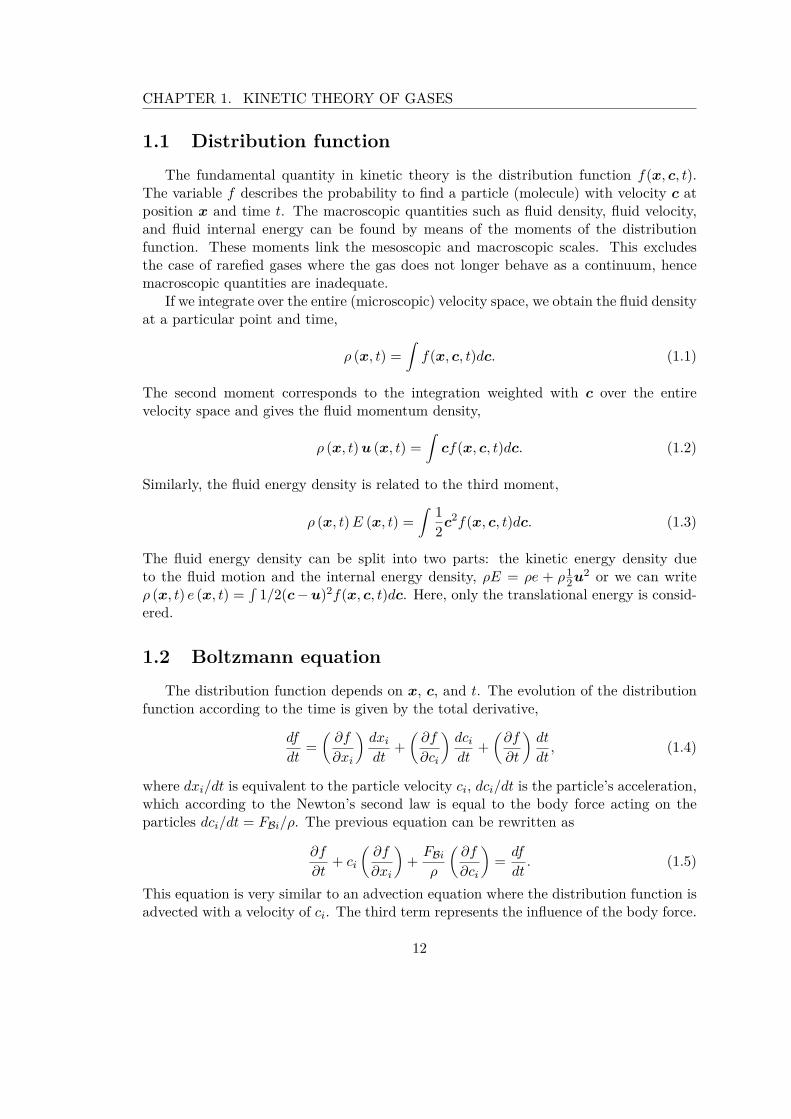
1.1 Distribution functionThe fundamental quantity in kinetic theory is the distribution function f(x, c, t).
The variable f describes the probability to find a particle (molecule) with velocity c atposition x and time t. The macroscopic quantities such as fluid density, fluid velocity,and fluid internal energy can be found by means of the moments of the distributionfunction. These moments link the mesoscopic and macroscopic scales. This excludesthe case of rarefied gases where the gas does not longer behave as a continuum, hencemacroscopic quantities are inadequate.
If we integrate over the entire (microscopic) velocity space, we obtain the fluid densityat a particular point and time,
ρ (x, t) =∫f(x, c, t)dc. (1.1)
The second moment corresponds to the integration weighted with c over the entirevelocity space and gives the fluid momentum density,
ρ (x, t) u (x, t) =∫
cf(x, c, t)dc. (1.2)
Similarly, the fluid energy density is related to the third moment,
ρ (x, t)E (x, t) =∫ 1
2c2f(x, c, t)dc. (1.3)
The fluid energy density can be split into two parts: the kinetic energy density dueto the fluid motion and the internal energy density, ρE = ρe + ρ1
2u2 or we can writeρ (x, t) e (x, t) =
∫1/2(c − u)2f(x, c, t)dc. Here, only the translational energy is consid-
ered.
1.2 Boltzmann equationThe distribution function depends on x, c, and t. The evolution of the distribution
function according to the time is given by the total derivative,
df
dt=(∂f
∂xi
)dxi
dt+(∂f
∂ci
)dci
dt+(∂f
∂t
)dt
dt, (1.4)
where dxi/dt is equivalent to the particle velocity ci, dci/dt is the particle’s acceleration,which according to the Newton’s second law is equal to the body force acting on theparticles dci/dt = FBi/ρ. The previous equation can be rewritten as
∂f
∂t+ ci
(∂f
∂xi
)+ FBi
ρ
(∂f
∂ci
)= df
dt. (1.5)
This equation is very similar to an advection equation where the distribution function isadvected with a velocity of ci. The third term represents the influence of the body force.
12

CHAPTER 1. KINETIC THEORY OF GASES
The right-hand side is similar to a source term and depicts the rate of change of thedistribution function df/dt due to collisions. The resulting equation is the Boltzmannequation and the right-hand side is called the collision operator. Using vector formulationyields to
∂f
∂t+ c · ∇f + FB
ρ· ∇cf =
(df
dt
)coll
, (1.6)
where ∇ is the gradient in the physical space and ∇c is the gradient in the velocityspace.
1.3 Collision operatorThe collision conserves the mass, the momentum, and the energy of particles, which
is equivalent to ∫ (df
dt
)coll
dc = 0, (1.7)∫c
(df
dt
)coll
dc = 0, (1.8)∫ 12c2
(df
dt
)coll
dc = 0; (1.9)
1, c, 12c2 are the collision invariants and results from the conservation laws of the system.
Using geometric considerations and assuming no correlations between particles priorto the collision (also known as molecular chaos approximation), the rate of change dueto the binary collision of particles takes the following form(
df
dt
)coll
=∫
(f1′f2′ − f1f2) gb db dϵ dc2, (1.10)
where f1 and f1′ refer to the distribution function of the first particle before and after thecollision. g is the initial relative speed of the two particles, b and ϵ are some geometricalquantities. More detailed explanations can be found in Ref. [1, 2] but for the sake ofsimplicity are not given here and are not necessary for the next developments.
1.3.1 Equilibrium
Let us consider the case of uniform conditions and absence of external forces, Eq. (1.6)becomes
∂f
∂t=∫
(f1′f2′ − f1f2) gb db dϵ dc2 (1.11)
A gas is at a local equilibrium state when the distribution function does not vary intime. This does not mean that particles sit idle and no collision occur but rather thatthe collisions do not change the distribution of gas particles. This leads to
feq1′ f
eq2′ = feq
1 feq2 . (1.12)
13

CHAPTER 1. KINETIC THEORY OF GASES
Taking the logarithm yields
ln(feq1′ ) + ln(feq
2′ ) = ln(feq1 ) + ln(feq
2 ). (1.13)
The logarithm of the distribution functions is a summational invariant of the collision.Thus it can be shown that the summational invariant must be a linear combination ofthe three collision invariants, so that
ln(feq) = A+ B · c − C12c2, (1.14)
where A, C are scalars, and B is a vector. They are independent of x, t since the stateof the gas is steady and uniform. This can be rewritten as
ln(feq) = lnD + 12C(c − 1
CB)2 (1.15)
feq = De12 C(c− 1
CB)2 (1.16)
feq = De− 12 Cc′2 (1.17)
where D is a new constant and c′ = c − 1C B. The unknown constant can be computed
by using the moments of the equilibrium distribution function. For the first moment,we have
ρ =∫feqdc = D
∫e− 1
2 Cc′2dc′. (1.18)
With the help of Gaussian integrals (∫∞
−∞ e−a(x+b)2dx =
√π/a), we obtain
ρ = D
∫ ∞
−∞e− 1
2 Cc′2dc′ = D
∫ ∞
−∞
∫ ∞
−∞
∫ ∞
−∞e− 1
2 C(c′2x +c′2
y +c′2z )dc′
xdc′ydc
′z (1.19)
ρ = D
(2πC
)3/2(1.20)
The second equilibrium moment is equivalent to
ρu =∫
cfeqdc (1.21)
ρu =∫ ∞
−∞(B/C + c′)feqdc′ (1.22)
ρu = ρB/C +D
∫ ∞
−∞c′e− 1
2 Cc′2dc′ (1.23)
u = B/C. (1.24)
The second integral term vanishes because the integrand is an odd function. This resultsto c′ = c − u. Using the definition of the internal energy of a monatomic gas at steady
14

CHAPTER 1. KINETIC THEORY OF GASES
state gives,
ρe = 32kBT
m=∫ 1
2(c − u)2feqdc (1.25)
32kBT
m= 1
2D∫ ∞
−∞c′2e− 1
2 Cc′2dc′ (1.26)
32kBT
m= 1
2D∫ ∞
−∞
∫ ∞
−∞
∫ ∞
−∞(c′2
x + c′2y + c
′2z )e− 1
2 C(c′2x +c
′2y +c
′2z )dc′
xdc′ydc
′z (1.27)
32kBT
m= 1
2D3C
(2πC
)3/2(1.28)
kBT
m= 1C
(1.29)
with kB the Boltzmann constant, T the temperature, and m the mass of one particleof gas. The following Gaussian integral
∫∞−∞ x2e−ax2
dx =√π/a/(2a) has been used to
compute the integral. Finally, we recover the famous Maxwell-Boltzmann equilibriumdistribution for a d (d = 3 in the previous derivation) dimensional space:
feq = ρ
(m
2πkBT
)d/2e
− m2kBT
(c−u)2(1.30)
= ρ
(2πRsT )d/2 e−(c−u)2/(2RsT ) (1.31)
where Rs = kB/m is the specific gas constant.
1.3.2 BGK collision operator
The complicated nonlinear integral collision operator Eq. (1.10) is often replacedby a simpler expression avoiding the inherent mathematical difficulties but resulting incorrect macroscopic behavior. Bhatnagar, Gross, and Krook propose the so-called BGKcollision operator [3], (
df
dt
)coll
= −1τ
(f − feq) (1.32)
where they introduced the relaxation time τ . This operator obeys to Eqs. (1.7),(1.8),(1.9) assuring the conservation of the mass, momentum and energy during the collision.One drastic simplification associated is the use of a relaxation time independent of thedistribution function f .
As an example, if we consider a gas whose distribution function is uniform in spacef(x, c, t) = f(c, t) but the gas is not at the equilibrium state at t = 0,
∂f(c, t)∂t
= −1τ
[f(c, t) − feq(c)] (1.33)
f(c, t) = feq(c) + (f(c, 0) − feq(c)) e−t/τ (1.34)
The distribution function relaxes exponentially to the equilibrium according to the typ-ical time-scale parameter τ .
15

CHAPTER 1. KINETIC THEORY OF GASES
1.4 Macroscopic balance equationsThe macroscopic conservation equations for the three invariants (mass, momentum,
and energy) can be derived from the Boltzmann equation Eq. (1.6).First, we introduce the following notation for the moments of f :
Π0 =∫fdc = ρ, Πi =
∫cifdc = ρui,
Πij =∫cicjfdc, Πijk =
∫cicjckfdc,
(1.35)
and so forth. These moments are unchanged if their indices are reordered, e.g, Πxyz =Πyxz. Concerning the force term, this next expression will be useful,∫
ψ∂f
∂cidc =
∫ ∫ψf dcjdck −
∫f∂ψ
∂cidc. (1.36)
The first term of this integration by parts, i.e., the surface integral, vanishes becausethe product ψf is assumed to diminish rapidly for large c [1, 4]. Integrating Eq. (1.6)multiplied by an arbitrary quantity ψ over c results in the Enskog’s general equation ofchange. In particular, the fundamental hydrodynamic equations of mass, motion, andenergy balance are recovered for ψ = 1, ci, cici.
Before the following preliminary result will be needed: equation (1.36) yields
∫∂f
∂cidc = 0, (1.37)∫
ci∂f
∂cjdc = −
∫∂ci
∂cjfdc = −ρδij , (1.38)∫
cici∂f
∂cjfdc = −
∫∂(cici)∂cj
dc = −2ρuj . (1.39)
Now, we now apply the moment "operator", i.e.,∫
•dc,∫ci • dc, and 1/2
∫cici • dc
(equivalent to ψ = 1, ci, 1/2cici) to the Boltzmann equation Eq. (1.6). If we integratethe Boltzmann equation over the velocity space, we get,
∂
∂t
∫fdc + ∂
∂xi
∫cifdc + FBi
ρ
∫∂f
∂cidc =
∫ (df
dt
)coll
dc. (1.40)
Note that the space and time derivatives have been moved out the integrals since t and xare not function of c. In addition, since velocity and space coordinates are independentvariables, ci∂f/∂xi = ∂(cif)/∂xi. Using Eqs. (1.1), (1.2), (1.7), and (1.37) gives thecontinuity equation,
∂ρ
∂t+ ∂(ρui)
∂xi= 0. (1.41)
If we multiply the Boltzmann equation Eq. (1.6) by ci and integrate over the velocityspace, we find,
∂
∂t
∫cifdc + ∂
∂xj
∫cicjfdc + FBj
ρ
∫ci∂f
∂cjdc =
∫ci
(df
dt
)coll
dc. (1.42)
16
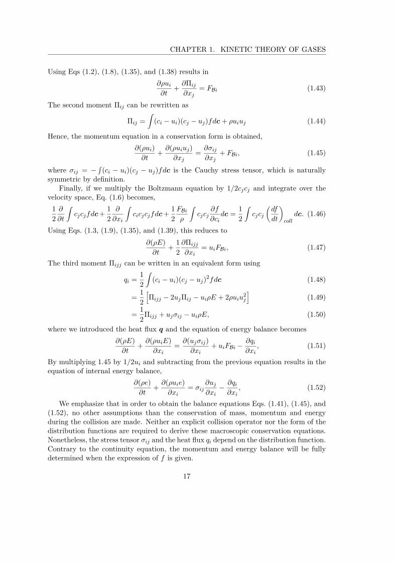
CHAPTER 1. KINETIC THEORY OF GASES
Using Eqs (1.2), (1.8), (1.35), and (1.38) results in∂ρui
∂t+ ∂Πij
∂xj= FBi (1.43)
The second moment Πij can be rewritten as
Πij =∫
(ci − ui)(cj − uj)fdc + ρuiuj (1.44)
Hence, the momentum equation in a conservation form is obtained,∂(ρui)∂t
+ ∂(ρuiuj)∂xj
= ∂σij
∂xj+ FBi, (1.45)
where σij = −∫
(ci − ui)(cj − uj)fdc is the Cauchy stress tensor, which is naturallysymmetric by definition.
Finally, if we multiply the Boltzmann equation by 1/2cjcj and integrate over thevelocity space, Eq. (1.6) becomes,
12∂
∂t
∫cjcjfdc + 1
2∂
∂xi
∫cicjcjfdc + 1
2FBi
ρ
∫cjcj
∂f
∂cidc = 1
2
∫cjcj
(df
dt
)coll
dc. (1.46)
Using Eqs. (1.3, (1.9), (1.35), and (1.39), this reduces to∂(ρE)∂t
+ 12∂Πijj
∂xi= uiFBi, (1.47)
The third moment Πijj can be written in an equivalent form using
qi = 12
∫(ci − ui)(cj − uj)2fdc (1.48)
= 12[Πijj − 2ujΠij − uiρE + 2ρuiu
2j
](1.49)
= 12Πijj + ujσij − uiρE, (1.50)
where we introduced the heat flux q and the equation of energy balance becomes∂(ρE)∂t
+ ∂(ρuiE)∂xi
= ∂(ujσij)∂xi
+ uiFBi − ∂qi
∂xi, (1.51)
By multiplying 1.45 by 1/2ui and subtracting from the previous equation results in theequation of internal energy balance,
∂(ρe)∂t
+ ∂(ρuie)∂xi
= σij∂uj
∂xi− ∂qi
∂xi, (1.52)
We emphasize that in order to obtain the balance equations Eqs. (1.41), (1.45), and(1.52), no other assumptions than the conservation of mass, momentum and energyduring the collision are made. Neither an explicit collision operator nor the form of thedistribution functions are required to derive these macroscopic conservation equations.Nonetheless, the stress tensor σij and the heat flux qi depend on the distribution function.Contrary to the continuity equation, the momentum and energy balance will be fullydetermined when the expression of f is given.
17

Chapter 2
Lattice Boltzmann method
Before presenting the lattice Boltzmann method (LBM), we recall that the classicalkinetic theory of gases is based on different assumptions, which can, to some extent,limit its applicability. First, we consider only binary collisions, thus this theory is notappropriate for dense gases and liquids where three-body collisions are significant. Nev-ertheless, Enskog and Eyring approximate theories have been proposed to deal withrespectively dense gases and liquids [1]. Second, the use of classical mechanics excludeslow-temperature phenomena where quantum effects are no longer negligible. Third, weimpose that the mean free path, i.e., the average distance traversed by a particle betweencollisions, is short compared to all macroscopic dimensions. Otherwise, the gas behavesas a discontinuous medium and the concept of local density, velocity, and energy losesmeaning. Fourth, monatomic spherical molecules are considered. In practice, the resultscan be also applied to polyatomic gases provided that a correction is added to take intoaccount the internal degrees of freedom and molecules are not too non-spherical.
What is the lattice Boltzmann method? The lattice Boltzmann method is a partic-ular discretization of the Boltzmann equation with a BGK, or an equivalent, collisionoperator. The lattice Boltzmann method can be derived in different ways. The firstroute is based on the kinetic theory of dilute gases and the discretization of the Boltz-mann equation (also called bottom-up or a posteriori approach). In the second routethe lattice Boltzmann method is constructed from a top-down or a priori strategy insuch a way that the Navier-Stokes equations are recovered using minimal mesoscopicrequirements. Both approaches are not equivalent but rather complementary. The firstway has a rigorous historical foundation from statistical mechanics. Due to its kineticrepresentation, mesoscopic effects can be directly modeled and hydrodynamics beyondthe Navier-Stokes equations can also be obtained [5]. However, this involves the afore-mentioned limitations, which seems to greatly restrict its applicability on hydrodynamicflows. On the contrary, the second way requires less unnecessary assumptions consider-ing a fluid parcel instead of a molecule of gas. The reader may have already noticed, wefollow the first route because of its fascinating physical insight and most importantly itprovides some expressions for the transport coefficients of gaseous mixtures as we willshow later. For the sake of brevity, we do not discuss the ancestor of the lattice Boltz-
19
CHAPTER 2. LATTICE BOLTZMANN METHOD
mann method: the lattice gas cellular automata. A concise presentation can be foundin Ref. [6]. Finally, a third noteworthy route begins directly from the discrete latticeBoltzmann equation, which is solely seen as a mesoscopic scheme for any distributionfunction with no relation with the Boltzmann equation. The number of discrete kineticvelocities and the equilibrium state are tailored to solve a particular partial differen-tial equation. This expands out the lattice Boltzmann method into a numerical solver.Hence, the lattice Boltzmann method has been employed to solve, to name a few, the lin-ear convection-diffusion equation [7] and nonlinear equations such as Ginzburg-Landau,Burgers-Fisher, nonlinear heat conduction, and sine-Gordon equations [8], or Burgers,Korteweg–de Vries, and Kuramoto–Sivashinsky equations [9], the wave equation [10],the shallow water equations [11].
In the following sections, the lattice Boltzmann method is derived from the Boltz-mann equation. The reader may ask why using the lattice Boltzmann method for solvingfluid flows instead of Navier-Stokes equations. Indeed for fluid dynamics, hydrodynamicquantities depend on the physical space x and the time t, and the microscopic velocitiesdo not appear in the fluids equations. The kinetic representation seems unnecessaryinvolving the time, the velocity space, and the physical space; yet in addition to its ap-pealing mesoscopic view of the flow, the lattice Boltzmann method has two other mainadvantages compared to the traditional way of solving Navier-Stokes equations. First,the advection in the Boltzmann equation, c · ∇f , is linear whereas the inertial term inthe Navier-Stokes equation is u · ∇u where u may be a complicated function of spaceand time. Secondly, the momentum diffusion in the lattice Boltzmann method is mate-rialized by the relaxation process of the BGK collision operator, which is non-linear butlocal. Because of these two advantages, as we will see, the resulting discrete equation isconceptually simple, efficient, and can easily be implemented on parallel architectures,while still being rigorously based on the kinetic theory of gases. These reasons mayexplain the rapid and growing interest in the lattice Boltzmann method for solving fluidflows.
2.1 Non-dimensional formulation
It is often convenient to use non-dimensional quantities and equations during mathe-matical manipulations. Let define a characteristic length l0, velocity v0, and density ρ0.The characteristic time scale is given by t0 = l0/v0. We introduce the non-dimensionalderivatives
∂
∂t⋆= l0v0
∂
∂t,
∂
∂x⋆i
= l0∂
∂xi,
∂
∂c⋆i
= v0∂
∂ci, (2.1)
where the stars denote non-dimensional quantities. The Boltzmann equation Eq. (1.6)is written in a non-dimensional form
∂f⋆
∂t⋆+ c⋆
i
(∂f⋆
∂x⋆i
)+ F ⋆
Bi
ρ⋆
(∂f⋆
∂c⋆i
)=(df
dt
)⋆
coll, (2.2)
20

CHAPTER 2. LATTICE BOLTZMANN METHOD
with f⋆ = vd0/ρ0f , ρ⋆ = ρ/ρ0, c⋆
i = ci/v0, F ⋆Bi = l0/v
20/ρ0FBi, and (df/dt)⋆
coll =vd
0/ρ0l0/v0 (df/dt)coll, and d is the number of spatial dimensions. Moreover, the equilib-rium distribution function has the following non-dimensional form
feq⋆ = ρ⋆
(2πθ⋆)d/2 e−(c⋆−u⋆)2/(2θ⋆), (2.3)
and θ∗ = RsT/v20 is the non-dimensional temperature. Henceforth, the star notation
will be omitted and all quantities will be non-dimensional unless otherwise stated.
2.2 Discretization of the velocity spaceUsually, there is no analytical solution of the continuum Boltzmann equation instead
the equation will be solved numerically. The distribution function spans over a seven-dimensional space: t, x, c, which has to be discretized. We first address the velocity spacediscretization. We point out that we are not interesting in the microscopic level of detailbut a correct macroscopic behavior of the flow. As we already saw, only the momentsof the distribution function appear in the macroscopic equations. As a result, we areonly looking for a discrete distribution function whose moments, weighted integrals, areequivalent to the moments of the continuous distribution function.
2.2.1 Hermite series
The distribution function can be expanded as a series of Hermite polynomials invelocity space c (see Appendix A and references [4, 5, 12] for more details)
f(x, c, t) = ω(c)∞∑
n=0
1n!a
(n)i (x, t)H(n)
i (c), (2.4)
with the following expansion coefficients and weight function
a(n)i (x, t) =
∫f(x, c, t)H(n)
i (c)dc, ω(c) = 1(2π)d/2 e
−c2/2. (2.5)
One of the nice features of this formulation is that all the expansion coefficients arelinear combinations of the moments of f . Substituting the Hermite polynomials by theirexpression Eqs. (A.16-A.19), we can identify the first few expansion coefficients with thehydrodynamic quantities
a(0) =∫fdc = ρ, (2.6)
a(1)i =
∫cifdc = ρui, (2.7)
a(2)ij =
∫(cicj − δij)fdc = Πij − δijρ = −σij + ρ(uiuj − δij), (2.8)
a(3)ijk =
∫(cicjck − ciδjk − cjδki − ckδij)fdc = Πijk − ρ(uiδjk + ujδki + ukδij). (2.9)
21

CHAPTER 2. LATTICE BOLTZMANN METHOD
We can limit the series Eq. (2.4) up to a certain order N . Also, the N -th expansioncoefficients are still valid by truncation of higher-order terms. Therefore, we consideronly the first N Hermite polynomials
fN (x, c, t) ≈ ω(c)N∑
n=0
1n!a
(n)i (x, t)H(n)
i (c). (2.10)
This is one of the reasons why the Hermite expansion is ingenious to describe the distri-bution function in the Boltzmann equation. Since the coefficients of the expansion arerelated to or coincide with the moments of f , i.e., the hydrodynamic quantities; onlya few truncated Hermite polynomials are needed to recover the relevant macroscopicphysics. This is the key idea of the Grad 13th-moments equations.
As previously, the equilibrium distribution function is also expanded. Noticing thatEq. (2.3) can be written in the following form
feq(x, c, t) = ρ
(√θ)d
ω
(c − u√
θ
), (2.11)
and using the change of variable ζ = (c − u)/√θ yield
a(n)eqi (x, t) = ρ
∫ω(ζ)H(n)
i (√θζ + u)dζ. (2.12)
The expression of the equilibrium expansion coefficients are known exactly and the firstfew equilibrium expansion coefficients read
a(0)eq = ρ
∫ω(ζ)dζ = ρ. (2.13)
Successive expressions are easily calculated using the orthogonality property of the Her-mite polynomials (see Eq. (A.20)). For instance,
a(1)eqi = ρ
∫ω(ζ)H(1)
i (√θζ + u)dζ (2.14)
= ρ
[√θ
∫ω(ζ)ζidζ + ui
∫ω(ζ)dζ
](2.15)
= ρ
[√θ
∫ω(ζ)H(1)
i (ζ)dζ + ui
](2.16)
= ρ
[√θ
∫ω(ζ)H(0)(ζ)H(1)
i (ζ)dζ + ui
](2.17)
= ρui, (2.18)
Similarly,
a(2)eqij = ρuiuj + ρ(θ − 1)δij , (2.19)
a(3)eqijk = ρuiujuk + ρ(θ − 1)(uiδjk + ujδki + ukδij). (2.20)
22

CHAPTER 2. LATTICE BOLTZMANN METHOD
The last term to expand (up to the N -th order) is related to the body forces. If wetake the derivative related to the velocity of Eq. (2.4) and use Eq. (A.14) successively,we have
∇cf(x, c, t) =N∑
n=0
1n!a
(n)i (x, t)∇c
(ω(c)H(n)
i (c))
(2.21)
=N∑
n=0
(−1)n
n! a(n)i (x, t)∇+1
c (ω(c)) (2.22)
= −ω(c)N∑
n=0
1n!a
(n)i (x, t)H(n+1)
i (c) (2.23)
= −ω(c)N∑
n=1
1(n− 1)!a
(n−1)i (x, t)H(n)
i (c). (2.24)
2.2.2 Gauss-Hermite quadrature
The last step is to evaluate the integrals in the expansion coefficients. If we truncatethe expansion of the distribution function as in Eq. (2.10), the integrand of Eq. (2.5)has the following form
fN (x, c, t)H(n)i (c) = ω(c)P (x, c, t), (2.25)
where P is a multi-dimensional polynomial in c of a degree not greater than 2N . AGauss-Hermite quadrature (see Appendix A) is of course employed to compute the ex-pansion coefficient
a(n)i (x, t) =
∫ω(c)P (x, c, t)dc =
qd∑α=0
ωαP (x, cα, t) =qd∑
α=0
ωα
ω(cα)fN (x, cα, t)H(n)
i (cα)
(2.26)with 2q − 1 ≥ 2N . Finally we define
fα(x, t) = ωα
ω(cα)fN (x, cα, t), (2.27)
and the moment of the distribution function are now
ρ =qd∑
α=1fα, (2.28)
ρui =qd∑
α=1cαifα, (2.29)
Πij =qd∑
α=1cαicαjfα, (2.30)
Πijk =qd∑
α=1cαicαjcαkfα. (2.31)
23

CHAPTER 2. LATTICE BOLTZMANN METHOD
The corresponding equation for fα is obtained by evaluating at cα the Boltzmann equa-tion, Eq. (1.6) and multiplying by ωα/ω(c),
∂fα
∂t+ cα · ∇f = −1
τ(fα − feq
α ) + Sα, (2.32)
where the BGK collision operator is employed to model collisions. The discrete equilib-rium feq
α is given by
feqα (x, t) = ωα
N∑n=0
1n!a
(n)eqi (x, t)H(n)
i (cα), (2.33)
and the effect of the body force is absorbed into the source term discrete Sα,
Sα(x, t) = FBρ
· ωα
N∑n=1
1(n− 1)!a
(n−1)i (x, t)H(n)
i (cα). (2.34)
2.3 Discrete velocity setsIn practice, most lattice Boltzmann implementations employ a Gauss-Hermite quadra-
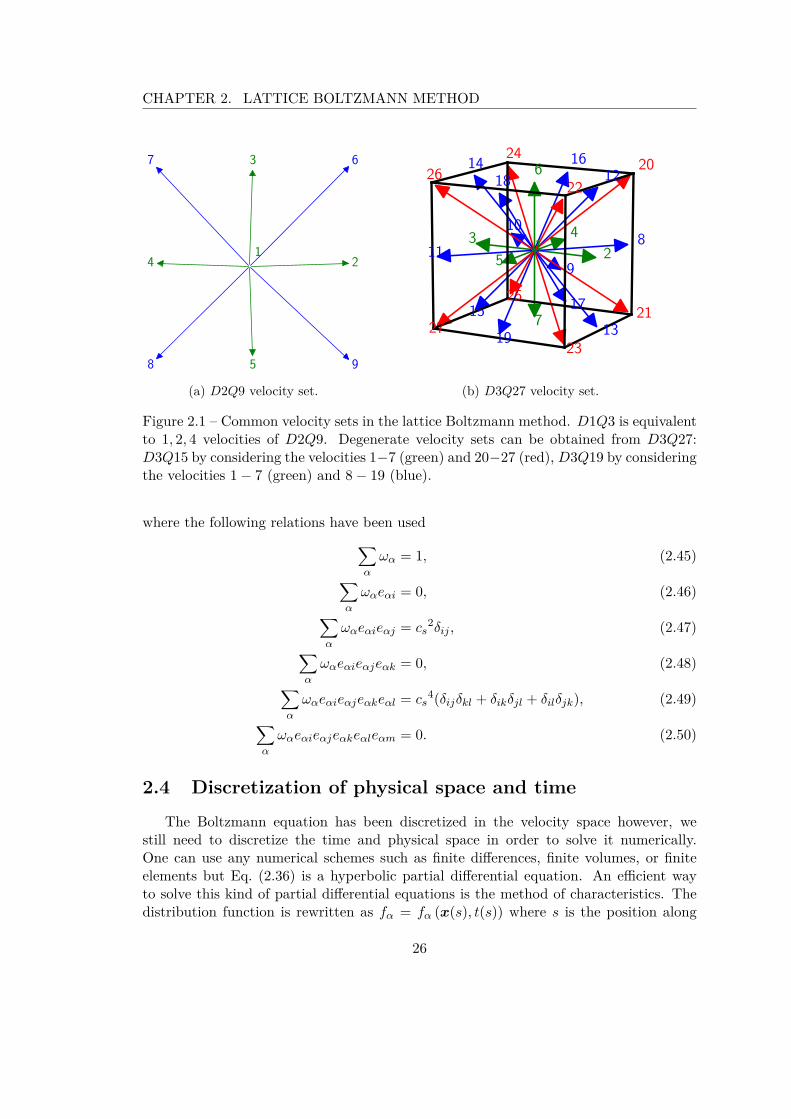
ture whose abscissas coincide with Cartesian coordinates. This corresponds to the ve-locity sets called D1Q3, D2Q9, D3Q15, D3Q19, and D3Q27; following the standardDdQq where d is the spatial dimension and q the number of velocities, i.e., abscissas.
All the previous quadratures are exact for a (multi-dimensional) polynomial of afifth-degree or less. That is why only the second-order Hermite terms have to be re-tained (5 ≥ 2N =⇒ N = 2). The third-order expansion coefficient a
(3)i is not conserved
by the truncation and the energy balance is no longer respected. Consequently, exclu-sively isothermal flows will be considered. Higher-order Gauss-Hermite quadratures arepossible but they are out of the scope of this thesis (D2Q17 and D3Q39 for a Cartesianuniform grid are exact quadratures for polynomials of a seventh-degree or less [5]).
If we set the non-dimensional temperature to θ = 1 and go back to the non-dimensional formulation Eq. 2.2, the characteristic velocity is v0 =
√RsT , which corre-
sponds to the speed of sound and the characteristic length is the distance traveled by asound wave in a unit of time. However, the abscissas in Appendix A contain a cumber-some
√3 factor so instead the characteristic length is scaled so as the lattice spacing is
equal to one. That is why a scaled abscissa eα is used in place of,
eα = cαcs, (2.35)
where the scaled factor is set to cs = c/√
3 with usually c = 1 and, as we will show, isrelated to the reference speed of sound. The resulting velocity sets are summarized inTable 2.1 and are drawn in Fig. 2.1.
Therefore, the non-dimensional quantities u, FB, and ∇ have also to be appropriatelyscaled by the factor cs and the resulting equations are
∂fα
∂t+ eα · ∇fα = −1
τ(fα − feq
α ) + Sα, (2.36)
24

CHAPTER 2. LATTICE BOLTZMANN METHOD
DdQq Velocities Weights
D1Q3 (0) 2/3(±1) 1/6
D2Q9(0, 0) 4/9
(±1, 0), (0,±1) 1/9(±1,±1) 1/36
D3Q15(0, 0, 0) 2/9
(±1, 0, 0), (0,±1, 0), (0, 0,±1) 1/9(±1,±1,±1) 1/72
D3Q19(0, 0, 0) 1/3
(±1, 0, 0), (0,±1, 0), (0, 0,±1) 1/18(±1,±1, 0), (±1, 0,±1), (0,±1,±1) 1/36
D3Q27
(0, 0, 0) 8/27(±1, 0, 0), (0,±1, 0), (0, 0,±1) 2/27
(±1,±1, 0), (±1, 0,±1), (0,±1,±1) 1/54(±1,±1,±1) 1/216
Table 2.1 – Common velocity sets used in the lattice Boltzmann method for cs = 1/√
3.If c = 1, velocities have to be multiplied by c.
where the equilibrium and the source terms are expanded up to the second-order
feqα = ρωα
[1 + u · eα
c2s
+ (u · eα)2
2c4s
− u · u
2c2s
], (2.37)
Sα = ωα
[eα − u
c2s
+ (eα · u)eα
c4s
]· FB. (2.38)
One can show that the moment of the equilibrium and the source term are given by
Πeq0 =
∑α
feqα = ρ,
∑α
Sα = 0, (2.39)
Πeqi =
∑α
eαifeqα = ρui,
∑α
eαiSα = FBi, (2.40)
and,
Πeqij =
∑α
eαieαjfeqα = ρcs
2δij + ρuiuj , (2.41)∑α
eαieαjSα = uiFBj + ujFBi, (2.42)
Πeqijk =
∑α
eαieαjeαkfeqα = ρcs
2(uiδjk + ujδki + ukδij), (2.43)∑α
eαieαjeαjSα = cs2(Fiδjk + Fjδki + Fkδij), (2.44)
25
CHAPTER 2. LATTICE BOLTZMANN METHOD
12
3
4
5
67
8 9
(a) D2Q9 velocity set.
12
3 4
5
6
7
8
9
10
11
12
13
14
15
16
17
18
19
20
21
22
23
24
25
26
27
(b) D3Q27 velocity set.
Figure 2.1 – Common velocity sets in the lattice Boltzmann method. D1Q3 is equivalentto 1, 2, 4 velocities of D2Q9. Degenerate velocity sets can be obtained from D3Q27:D3Q15 by considering the velocities 1−7 (green) and 20−27 (red), D3Q19 by consideringthe velocities 1 − 7 (green) and 8 − 19 (blue).
where the following relations have been used∑α
ωα = 1, (2.45)∑α
ωαeαi = 0, (2.46)∑α
ωαeαieαj = cs2δij , (2.47)∑
α
ωαeαieαjeαk = 0, (2.48)∑α
ωαeαieαjeαkeαl = cs4(δijδkl + δikδjl + δilδjk), (2.49)∑
α
ωαeαieαjeαkeαleαm = 0. (2.50)
2.4 Discretization of physical space and time
The Boltzmann equation has been discretized in the velocity space however, westill need to discretize the time and physical space in order to solve it numerically.One can use any numerical schemes such as finite differences, finite volumes, or finiteelements but Eq. (2.36) is a hyperbolic partial differential equation. An efficient wayto solve this kind of partial differential equations is the method of characteristics. Thedistribution function is rewritten as fα = fα (x(s), t(s)) where s is the position along
26

CHAPTER 2. LATTICE BOLTZMANN METHOD
the characteristic line (x(s), t(s)). Along these characteristics, the partial differentialequation reduces to an ordinary differential equation,
dfα
ds= ∂fα
∂t
dt
ds+ ∂fα
∂xi
dxi
ds= −1
τ(fα − feq
α ) + Sα. (2.51)
This previous equation is equivalent to the discrete velocity Boltzmann equation Eq. (2.36)if
dt
ds= 1, dxi
ds= eαi. (2.52)
Letting t(0) = t and xi(0) = xi, we find t(s) = t+ s and xi(s) = x+ eαis. We integrateEq. (2.51) over a time step, from s = 0 to s = δt,
fα(x+eαδt, t+ δt) − fα(x, t) =∫ δt
0
−1τ
[fα(x + eαs, t+ s) − feqα (x + eαs, t+ s)] + Sα(x + eαs, t+ s)
ds
(2.53)
The integral is evaluated using the trapezoidal rule.
fα(x+eαδt, t+ δt) − fα(x, t) =
− δt
2τ [fα(x + eαδt, t+ δt) − feqα (x + eαδt, t+ δt) + fα(x, t) − feq
α (x, t)]
+ δt
2 [Sα(x + eαδt, t+ δt) + Sα(x, t)] (+O(δt3))
(2.54)
This is a second-order accurate discretization but the resulting equation is implicit. Ifwe introduce the change of variable
fα = (1 + δt
2τ )fα − δt
2τ feqα − δt
2 Sα, (2.55)
the previous equation gives
fα(x + eαδt, t+ δt) = fα(x, t) − δt
τ
[fα(x, t) − feq
α (x, t)]
+ δt(1 − δt
2τ )Sα, (2.56)
with feqα = feq
α and τ = τ + δt/2. Surprisingly, with this change of variable, the equa-tion becomes explicit and is second-order accurate despite having a similar form as afirst-order discretization. This is another interesting property of the lattice Boltzmannmethod. The macroscopic quantities are obtained by computing the moment of fα:∑
α
fα = ρ, (2.57)
∑α
eαfα = ρu − δt
2 FB, (2.58)
and similarly, other quantities can be directly calculated from fα. Hence and from now,the ˆ notation will be omitted, and fα and τ will refer to the transformed variables.
27

CHAPTER 2. LATTICE BOLTZMANN METHOD
In the lattice Boltzmann method, a convenient system of units called lattice units(lu) is commonly employed. In this system, the time and space steps are set equal toone. Conversion factors and non-dimensional numbers are then used to compare thesimulation with experimental or numerical results. For instance, in lattice units weusually set δxLBM = 1, δtLBM = 1, and ρLBM = 1 whereas in physical system we haveδxphy, δtphy, and ρphy. The conversion factors from the lattice units to the physicalsystem are simply for the length Cl = δxphy, the time Ct = δtphy and density Cρ = ρphy.We emphasize that whatever the system of units is considered all the dimensionlessnumbers are equal. Let consider for example the Mach number
Ma = Uphy
cphy= ULBM
cs, (2.59)
= Uphy
ULBM= Cl
Ct= δxphy
δtphy= cphy
cs=
√3 × cphy. (2.60)
In consequence, setting the Mach number gives a relationship between the physical spaceand time steps of the simulation Ma = δxphy/δtphy = cphy
√3.
Finally, the lattice Boltzmann method can be split into two main steps and is sum-marized below:
f∗α(x, t) = fα(x, t) − 1
τ[fα(x, t) − feq
α (x, t)] + (1 − 12τ )Sα Collision, (2.61)
fα(x + eα, t+ 1) = f∗α(x, t) Streaming, (2.62)
with
ρ =∑
α
fα, feqα = ρωα
[1 + u · eα
c2s
+ (u · eα)2
2c4s
− u · u
2c2s
], (2.63)
ρu =∑
α
eαfα + 12FB, Sα = ωα
[eα − u
c2s
+ (eα · u)eα
c4s
]· FB. (2.64)
The first step is called collision and is purely local. The formulation of the source termexpressed up to the second-order is the same as Guo’s forcing scheme [13] obtaineda priori so as to derive the correct Force expression in the Navier-Stokes equations.The second step is the streaming, which propagates the distribution functions to theneighboring lattice points. The advantage of a quadrature whose abscissas coincide withthe Cartesian coordinates is evident. If x belongs to a lattice node, then x + eα isalso a lattice point. The streaming step is just a shift of the post-collision distributionfunctions to the next lattice nodes. The advection is exact, there is no diffusion addedby the use of an interpolation scheme for instance. The implementation of the algorithmis straightforward (see Algo. 1 and Fig. 2.2).
The final result is conceptually simple yet physically based on the kinetic theory ofgases. The algorithm is very efficient as all steps but the streaming are local and thenon-locality (propagation) is just a shift in the memory involving the next neighboredlattice nodes. Moreover, the code can easily be parallelized and achieves high per-formance on multi-core computers. For instance, using the Message-Passing Interface
28

CHAPTER 2. LATTICE BOLTZMANN METHOD
while t ≤ tmax docollide;do MPI communications;stream;apply boundary conditions;compute moments and force, ρ, ρu, FB;t = t+ δt;
endAlgorithm 1: Lattice Boltzmann algorithm
(MPI) paradigm, the computational domain is expanded with a layer of ghost nodes.These ghost nodes store a copy of the neighboring node from the adjacent MPI processand are updated just before the streaming step as shown in Algo. 1 since other steps arelocal. More details concerning programming considerations can be found in Appendix B.
2.5 Chapman and Enskog expansion procedureAs we know, the order of expansion of the Hermite series predicts which moments
we can exactly recover from the truncation of higher orders. However, the macroscopicequations are not completely closed and the expression of Πij , for instance, in terms ofhydrodynamic quantities is still required. We need a way to assess the level of accuracyover the different scales of the physics. The Chapman and Enskog expansion estimates,from the deviation of the equilibrium, the relevant physical scales that are solved. Thedistribution functions are expanded in terms of powers of the Knudsen number [2]:
fα = f (0)α + Kf (1)
α + K2f (2)α + · · · , (2.65)
where K is the Knudsen number, i.e., the mean free path divided by the characteristiclength of the flow. The source term is often expanded as Sα = KS(1)
α , where higher-order terms are not generally required to obtain the correct macroscopic equations.For usual fluid flows with slow time and large spatial scales variations, the Knudsennumber is small. The fluid behaves like a continuum and the Navier-Stokes descriptionis valid. In other cases, such as in microfluidics, or rarefied gases, the Knudsen numberis large (K ≥ 0.1) and higher orders are required in the expansion of Eq. (2.65) todescribe phenomena beyond the Navier-Stokes level. Time and spatial variations arealso expanded in terms of powers of K [2] as follow:
∂
∂t= ∂t = K∂(1)
t + K2∂(2)t + · · · , and ∂
∂xi= ∂i = K∂(1)
i (2.66)
Using this appropriate division of the derivatives is necessary because fα is unknown andso as the momentum flux Πij . The determination of fα by successive approximationsis difficult because, as we will see, the time derivative of the hydrodynamics variablesdetermines the time derivative of f (0)
α , on which the equation from which f (1)α is inferred
29

CHAPTER 2. LATTICE BOLTZMANN METHOD
(a) Collision step. (b) Streaming step.
Figure 2.2 – Sketch of the collision and streaming step for the node B2 with the D2Q9velocity set. Notice that f0 associated with the vector (0, 0) is not represented. Thecollision involves all the distribution functions from the node, after the streaming steppropagates the distribution functions to the neighbor nodes according to the directioneα.
depends. The expansion of the time derivative proposed by Enskog allows to circumventthis difficulty [2].
We now apply the Chapman and Enskog expansion to the lattice Boltzmann equationEqs. (2.61) and (2.62), nevertheless the expansion can also be applied to the Boltzmannequation [Eq. (1.6)] or its counterpart discretized in the velocity space [Eq. (2.36)].Starting from
fα(x + eα, t+ δt) = fα(x, t) − δt
τ[fα(x, t) − feq
α (x, t)] + δt(1 − δt
2τ )Sα (2.67)
The Taylor expansion up to the second-order of fα(x + eα, t+ δt) gives
fα(x + eα, t+ δt) − fα(x, t) = δt (∂t + eαi∂i) fα + δt2
2 (∂t + eαi∂i)2 fα +O(δt3) (2.68)
Applying this Taylor expansion to Eq. (2.67) and using the expansions of Eqs. (2.65)and (2.66), the resulting equation can be separated according to the different order ofK:O(K0) :
f (0)α = feq
α , (2.69)
O(K1) : (∂
(1)t + eαi∂
(1)i
)f (0)
α = −1τf (1)
α + (1 − δt
2τ )S(1)α , (2.70)
30

CHAPTER 2. LATTICE BOLTZMANN METHOD
O(K2) :
∂(2)t f (0)
α +(∂
(1)t + eαi∂
(1)i
)f (1)
α + δt
2(∂
(1)t + eαi∂
(1)i
)2f (0)
α = −1τf (2)
α . (2.71)
With the help of Eq. (2.70), the equation for the second-order O(K2) is rewritten as
∂(2)t f (0)
α +(∂
(1)t + eαi∂
(1)i
)(1 − δt
2τ
)(f (1)
α + δt
2 S(1)α
)= −1
τf (2)
α . (2.72)
A very important remark from the observation of the equations of different orders ofK is the fact that we need the previous order f (k)
α to compute f (k+1)α . If we discard the
source term for the sake of simplicity, we can write
f (k+1)α = −τ
⎡⎣ k∑β=0
∂(k)t f (β)
α + bkeα · ∇f (k)α
⎤⎦ , (2.73)
where bk is an artefact due to the spatial and temporal discretization, e.g., b2 = (1−δt/2).If we recall the Hermite series of f up to order N , the term eα ·∇f need an expansion oforder N+1 in order to be described appropriately (see the recurrence relation Eq. (A.7)).That means if we want to correctly describe a flow at order O(Kk), the equilibrium andthe distribution function have to be expanded up to order N + k in the Hermite series.For the aforementioned quadratures of fifth-degree, N = 2. Recalling that the Hermiteexpansion coefficient of order N is a linear combination of the moment of the distributionfunction up to the order N ; the zeroth, first, and second moments of f (k=0) are accuratelydepicted and so as the zeroth, first moments of f (k=1). That is why we can expect anerror from the second moment of f (k=1) which is related to the pressure tensor in theNavier-Stokes equation as we will show shortly.
As expected, the Chapman and Enskog expansion analyses the asymptotic behav-ior of the (lattice) Boltzmann equation according to the deviation of the distributionfunctions from the equilibrium. Since f (0)
α = feqα , we have∑
α
fα = ρ =∑
α
feqα =
∑α
f (0)α =⇒
∑α
f (n)α = 0 ∀n ≥ 1, (2.74)
and ∑α
eαifα = ρui − δt
2 FBi∑α
eαifeqα =
∑α
eαif(0)α = ρui
⎫⎪⎪⎪⎬⎪⎪⎪⎭ =⇒
⎧⎪⎪⎪⎨⎪⎪⎪⎩∑
α
eαif(1)α = −δt
2 FBi∑α
eαif(n)α = 0 ∀n ≥ 2
(2.75)
where the right-hand side is consequence of the expansion Sα = KS(1)α .
Let focus now on the order O(K). Taking the zeroth, first, and second moments ofEq. (2.70) yields
∂(1)t ρ+ ∂
(1)i (ρui) = 0, (2.76)
∂(1)t (ρui) + ∂
(1)j Πeq
ij = FBi, (2.77)
∂(1)t Πeq
ij + ∂(1)k Πeq
ijk = −1τ
Π(1)ij + (1 − δt
2τ )(uiFBj + ujFBi), (2.78)
31

CHAPTER 2. LATTICE BOLTZMANN METHOD
with Πeqij = ρuiuj + ρcs
2δij . The first two equations corresponds to the Euler equationswhere the pressure is defined as p = ρcs
2. Similarly, computing the zeroth and firstmoments of Eq. (2.72) gives
∂(2)t ρ = 0, (2.79)
∂(2)t (ρui) + ∂
(1)j
(1 − δt
2τ )[Π(1)
ij + δt
2 (uiFBj + ujFBi)]
= 0. (2.80)
Π(1)ij is still unknown but can be expressed using the equations at order O(K):
Π(1)ij = −τ
[∂
(1)t Πeq
ij + ∂kΠeqijk − (1 − δt
2τ )(uiFBj + ujFBi)]. (2.81)
Recalling that ∂i(abc) = a∂i(bc) + b∂i(ac) − ab∂i(c), we have
∂(1)t Πeq
ij = ∂(1)t
[ρuiuj + ρcs
2δij
]= ui∂
(1)t (ρuj) + uj∂
(1)t (ρui) − uiuj∂
(1)t ρ+ cs
2δij∂(1)t ρ
= −ui
[∂
(1)k (ρujuk + ρcs
2δjk) − FBj
]− uj
[∂
(1)k (ρuiuk + ρcs
2δki) − FBi
]+ uiuj∂
(1)k (ρuk) − cs
2δij∂(1)k (ρuk)
= −[ui∂
(1)k (ρujuk) + uj∂
(1)k (ρuiuk) − uiuj∂
(1)k (ρuk)
]+ uiFBj + ujFBi
− cs2(ui∂
(1)j ρ+ uj∂
(1)i ρ
)− cs
2δij∂(1)k (ρuk)
= −∂(1)k (ρuiujuk) + uiFBj + ujFBi
− cs2(ui∂
(1)j ρ+ uj∂
(1)i ρ
)− cs
2δij∂(1)k (ρuk),
and
∂(1)k Πeq
ijk = ∂k
[ρcs
2(uiδjk + ujδki + ukδij)]
= cs2[∂
(1)j (ρui) + ∂
(1)i (ρuj)
]+ cs
2δij∂(1)k (ρuk).
Finally, we get
Π(1)ij = −τ
[ρcs
2(∂(1)j ui + ∂
(1)i uj) − ∂
(1)k (ρuiujuk) + δt
2τ (uiFBj + ujFBi)]. (2.82)
The equation Eq. (2.80) can now be written explicitly
∂(2)t (ρui) + ∂
(1)j
−τ(1 − δt
2τ )[ρcs
2(∂(1)j ui + ∂
(1)i uj) − ∂
(1)k (ρuiujuk)
]= 0. (2.83)
32
CHAPTER 2. LATTICE BOLTZMANN METHOD
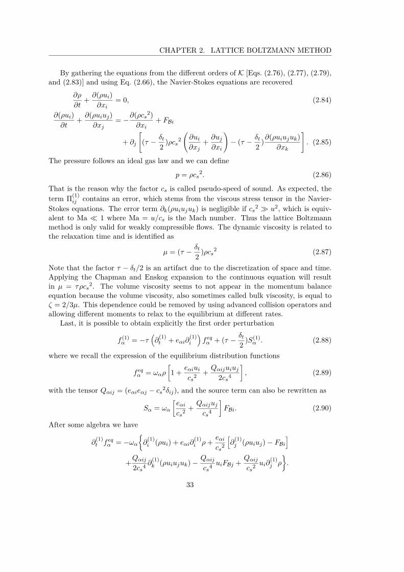
By gathering the equations from the different orders of K [Eqs. (2.76), (2.77), (2.79),and (2.83)] and using Eq. (2.66), the Navier-Stokes equations are recovered
∂ρ
∂t+ ∂(ρui)
∂xi= 0, (2.84)
∂(ρui)∂t
+ ∂(ρuiuj)∂xj
= −∂(ρcs2)
∂xi+ FBi
+ ∂j
[(τ − δt
2 )ρcs2(∂ui
∂xj+ ∂uj
∂xi
)− (τ − δt
2 )∂(ρuiujuk)∂xk
]. (2.85)
The pressure follows an ideal gas law and we can define
p = ρcs2. (2.86)
That is the reason why the factor cs is called pseudo-speed of sound. As expected, theterm Π(1)
ij contains an error, which stems from the viscous stress tensor in the Navier-Stokes equations. The error term ∂k(ρuiujuk) is negligible if cs
2 ≫ u2, which is equiv-alent to Ma ≪ 1 where Ma = u/cs is the Mach number. Thus the lattice Boltzmannmethod is only valid for weakly compressible flows. The dynamic viscosity is related tothe relaxation time and is identified as
µ = (τ − δt
2 )ρcs2 (2.87)
Note that the factor τ − δt/2 is an artifact due to the discretization of space and time.Applying the Chapman and Enskog expansion to the continuous equation will resultin µ = τρcs
2. The volume viscosity seems to not appear in the momentum balanceequation because the volume viscosity, also sometimes called bulk viscosity, is equal toζ = 2/3µ. This dependence could be removed by using advanced collision operators andallowing different moments to relax to the equilibrium at different rates.
Last, it is possible to obtain explicitly the first order perturbation
f (1)α = −τ
(∂
(1)t + eαi∂
(1)i
)feq
α + (τ − δt
2 )S(1)α . (2.88)
where we recall the expression of the equilibrium distribution functions
feqα = ωαρ
[1 + eαiui
cs2 + Qαijuiuj
2cs4
], (2.89)
with the tensor Qαij = (eαieαj − cs2δij), and the source term can also be rewritten as
Sα = ωα
[eαi
cs2 + Qαijuj
cs4
]FBi. (2.90)
After some algebra we have
∂(1)t feq
α = −ωα
∂
(1)i (ρui) + eαi∂
(1)i ρ+ eαi
cs2
[∂
(1)j (ρuiuj) − FBi
]+Qαij
2cs4 ∂
(1)k (ρuiujuk) − Qαij
cs4 uiFBj + Qαij
cs2 ui∂
(1)j ρ
.
33

CHAPTER 2. LATTICE BOLTZMANN METHOD
The two last terms have been simplified by using the symmetry property of the ten-sor, i.e., QαijRij = QαijRji for any tensor Rij . The spatial partial derivative of theequilibrium reads
eαi∂(1)i feq
α = ωα
[eαi∂
(1)i ρ+ eαieαj
cs2 ∂
(1)i (ρuj) + eαi
Qαjk
2cs4 ∂
(1)i (ρujuk)
].
And if we combine the two previous equations, Eq. (2.88) becomes
f (1)α = −τωα
cs2
[ρQαij∂
(1)i uj − eαi∂
(1)j (ρuiuj) + Qαij
2cs2 eαk∂
(1)k (ρuiuj)
−Qαij
2cs2 ∂
(1)k (ρuiujuk)
]− δtωα
2cs2
[eαiFBi + Qαij
cs2 ujFBi
] (2.91)
This is an important result, which highlights the fact that the non-equilibrium part ofthe distribution function is mainly related to the gradient of u and u, FB in the case ofa flow subject to a body force.
To conclude, the Chapman and Enskog procedure is an asymptotic expansion interms of powers of the Knudsen number and allows us to identify the macroscopic balanceequations involved. Closed to the equilibrium at order O(K), the Euler equations arerecovered. At second-order O(K2), the Navier-Stokes equations are obtained. Due toan insufficient quadrature, a small error appears in the viscous stress tensor and thelattice Boltzmann method is usually used in the case of weakly (isothermal) compressibleflows. Of course, increasing the order of the quadrature is possible in order to solvethermal flows and observe phenomena beyond the Navier-Stokes level (Burnett andsuper-Burnett equations). The Chapman and Enskog expansion is an important tool tolink the mesoscopic and macroscopic scales. In our cases, this provides a relationshipbetween the relaxation time of the distribution function toward the equilibrium and theviscosity. Other alternative multi-scales approaches [14, 15, 16] are also possible andresults in similar (compressible or incompressible) Navier-Stokes equations.
2.6 Advanced collision operators
The expression of the viscosity according to the relaxation time gives a necessarycondition for the stability of the lattice Boltzmann method: τ ≥ 1/2 in order to have apositive viscosity. In fact, the lattice Boltzmann method is prone to numerical instabil-ities when τ is close to 1/2. The BGK collision operator and the exact streaming makethe LBM very little dissipative [17]. Hence, numerical errors and small pressure wavesare not naturally damped causing stability issues, and simulating high Reynolds numberflows challenging. Notice that the error term in the stress tensor has a negative effect bydecreasing the viscous dissipation. However, this error seems to not be the major cause.In fact, a von Neumann linear analysis suggests that the instability occurs when somemodes interact with each other [18]. That is why a higher-order quadrature (D2Q17) isfound to be theoretically more unstable even though there is no error in the stress tensor
34

CHAPTER 2. LATTICE BOLTZMANN METHOD
because the number of modes increases and consequently their possibility of interactiontoo. Nonetheless, the roots of the instability of the Lattice Boltzmann method are notcompletely understood and remain, as well as strategies to remedy these stability de-fects, an active research topic. In the next paragraph, we will briefly present the mostcommon advanced collision operators used to improve the stability of the scheme.
2.6.1 Multiple relaxation time
As we learned from the Chapman and Enskog expansion, the viscous dissipationis related to the relaxation process of the second moment Πij . In the BGK collisionoperator, the distribution functions relax toward the equilibrium according to a singlerelaxation time. A more sophisticated idea is to relax each moment according to a properrelaxation time. This method is called multiple relaxation time (MRT). We introducethe matrix M, which transforms the distribution functions into moments:
mα = Mfα. (2.92)
M is a square transformation matrix. If the first line of the matrix is filled only by1, then the first moment is the density. The invert transformation from the momentsto distribution functions is simply fα = M−1mα. The main idea is to perform thecollision step in the moment space, namely relax each moment with individual relaxationtime, transformed back the relaxed moments to the population and stream as usual.Eqs. (2.61) and (2.62) are rewritten as
m∗α(x, t) = mα(x, t) − S [mα(x, t) −meq
α (x, t)] + (I − 12S)MSα (2.93)
fα(x + eα, t+ 1) = M−1m∗α(x, t), (2.94)
where I is the identity, and S is the diagonal matrix corresponding to the inverse ofthe relaxation time associated with each moment. Notice that the equilibrium momentsare obtained from meq
α = Mfeqα and the source term is also expressed in the moment
space. Each line of the matrix M defines a moment. To construct the transformationmatrix, the only condition is the rows of the matrix should be linearly independent(M has to be an invertible matrix). Hence there is no unique transformation matrix.One can choose to construct the matrix according to the Hermite polynomials howeverthe common approach is based on a Gram-Schmidt procedure of a combination of thevelocity vector eα. In both cases, the rows of M are orthogonal with respect to theweight ωα for the Hermite polynomials and with weight equal to unity for the Gram-Schmidt procedure. In the case the D2Q9 velocity set, M is usually obtained from thefollowing nine polynomials
1 x y xy x2 + y2 x2 − y2 x(x2 + y2) y(x2 + y2) (x2 + y2)2. (2.95)
Let Mi− the i-th row of M and eαx, eαy are the component of the velocity vector eα.The density, the momentum according to x and y-axes correspond respectively to ||e||0
35

CHAPTER 2. LATTICE BOLTZMANN METHOD
(M1−), eαx (M4−), and eαy (M6−). These three vectors constitute the eigenvectors ofthe MRT collision operator. Then the second line M2− is obtained by using a Gram-Schmidt procedure on ||eα||2. In the same way M5− and M7− are constructed by theorthogonalization of respectively eαx||eα||2 and eαy||eα||2, M8− comes from e2
αx − e2αy
and M9− is built from eαxeαy. Finally, M3− is obtained from ||eα||4. The matrix Mreads [19]
M =
⎛⎜⎜⎜⎜⎜⎜⎜⎜⎜⎜⎜⎜⎜⎜⎝
1 1 1 1 1 1 1 1 1−4 −1 −1 −1 −1 2 2 2 2
4 2 2 2 2 1 1 1 10 1 0 −1 0 1 −1 −1 10 −2 0 2 0 1 −1 −1 10 0 1 0 −1 1 1 −1 −10 0 −2 0 2 1 1 −1 −10 1 −1 1 −1 0 0 0 00 0 0 0 0 1 −1 1 −1
⎞⎟⎟⎟⎟⎟⎟⎟⎟⎟⎟⎟⎟⎟⎟⎠. (2.96)
The lines of the matrix are ordered by starting with the three scalars, then the fourvectors and finally the two tensors components. The vectors were multiplied by someconstants in order to have some handy integer expressions. The moments are relatedto some macroscopic quantities. m1 is the fluid density ρ, m2 and m3 are proportionalto the kinetic energy and the square of the kinetic energy, respectively. m4 and m6are equivalent to ρux and ρuy. m5 and m7 are proportional to x and y-components ofthe heat flux. Finally, m8 and m9 are proportional respectively to the diagonal andoff-diagonal terms of the viscous stress tensor. The diagonal of S corresponds to theinverse of the relaxation time, also called relaxation rate, associated with each moment
S = diag (0, sE , sζ , 0, sq, 0, sq, sµ, sµ) (2.97)
Note that using the polynomials x2 +y2, x2 −y2 instead of x2, y2 makes S to be diagonalif one wants to decouple ζ and µ [20]. If the Chapman-Enksog expansion is applied tothe lattice Boltzmann equation with the MRT collision operator, one finds
µ = ( 1sµ
− 12)ρcs
2 (2.98)
ζ = ( 1sζ
− 12)ρcs
2 − µ
3 (2.99)
With a relaxation rate associated with each moment (some are equal to enforce isotropy),the volume viscosity can now be independently set. For high Reynolds number flows, thevolume viscosity is generally artificially increased, which helps with the dissipation ofpressure waves being potential sources of instability. Since the density and momentumare conserved by the collision, the value of their relaxation rate has no influence and isset to zero. sµ is related to the dynamic viscosity. The other relaxation rates, sE and sq
for D2Q9, do not appear in the macroscopic equations. These two free parameters canbe tuned to improve the accuracy and the stability of the scheme. The BGK operatoris recovered if all the relaxation rates are the same.
36
CHAPTER 2. LATTICE BOLTZMANN METHOD
There is no systematic procedure to choose the relaxation rates that do not appearin the macroscopic equations. It is often a compromise between accuracy and stability.Notice that the application of the MRT collision operator for three-dimensional flows(D3Q15, D3Q19, andD3Q27) is straightforward [21] and there are more free parameters,relaxation rates, to adjust. We will now discuss on reduced MRT model with onlytwo relaxation time (TRT), one related to the dynamics viscosity corresponding to themoments constructed with the even-order velocity polynomials (sE = sζ = sµ = s+)and the other one is a free parameter corresponding to the moments constructed withthe odd-order velocity polynomials (sq = s−). In addition to providing a simple and afast way to choose the relaxations rates, the accuracy error becomes independent of theviscosity if the so-called magic number Λ remains constant [22]
Λ+− =( 1s+
− 12
)( 1s−
− 12
). (2.100)
The specific choice of Λ = 3/16 corresponds to sq = 82−s+
8−s+ . In the case of a Poiseuilleflow in a straight channel, the boundary implemented with the bounce-back condition(explanations are given later at section 2.7.3) is located exactly in the middle betweena fluid node and a solid (wall) node. As a general rule, Λ ∈ [1/8, 3/8] allows reasonablyaccurate results for flows in porous media [23, 24].
2.6.2 Central moments
The central moment method is an extension of the MRT collision model. As wepreviously mentioned, in MRT the transformation matrix is not unique. In the centralmoment collision operator, M is constructed using polynomials in (eα − u) instead ofeα. This enhances the Galilean invariance and stability. However the matrix M has tobe inverted at each time step, in each grid point since the matrix is no longer constantand depends on the velocity of the fluid. This greatly increases the computational costof the algorithm. Two different algorithms can be found in the literature. The cascadedoperator refers to the use of an orthogonal basis for the construction of the transformationmatrix, and the moments relax to the continuous Maxwellian equilibrium. Otherwise,central moments are generally based on a non-orthogonal basis and relax to the standarddiscrete equilibrium. Since the choice of the polynomials sometimes differ and resultin different transformation matrices, the comparison between models is complicated.Extensive details are available in Ref. [25] and recent advances in Ref. [26].
2.6.3 Cumulant
The cumulant collision operator follows the same main principle of relaxing somequantities, cumulants instead of moments of the distribution functions. The cumulantscan be computed from a non-linear combination of central moments. This results in abetter Galilean invariance and more stable results [27] but the scheme becomes compli-cated and especially more computationally intensive than the central moments collisionoperator.
37

CHAPTER 2. LATTICE BOLTZMANN METHOD
2.6.4 Regularized
The regularized collision operator is based on a simple idea that the instabilities stemfrom the high order terms in the Chapman-Enksog expansion. At each interation, beforecollision, the distribution function is regularized as follow [28]
f regα = feq
α + f (1)α (2.101)
Thus the distribution function does not contain any unnecessary high order terms at theNavier-Stokes level which may worsen the stability of the scheme. From the Chapmanand Enskog expansion Eq. (2.91), one finds
f (1)α ≈ − ωα
2cs2
[τρQαij(∂ui
∂xj+ ∂uj
∂xi) − τ
Qαij
cs2∂
xk(ρuiujuk)
]− δt
2 Sα. (2.102)
Notice that we could use directly Eq. (2.91) and evaluate the derivatives by finite dif-ference however the regularized collision operator would not be local anymore and thusbecomes computationally very expensive. We recall Eq. (2.82)
Πneqij ≈ Π(1)
ij = −τ[ρcs
2(∂(1)j ui + ∂
(1)i uj) − ∂
(1)k (ρuiujuk)
]− δt
2 (uiFBj + ujFBi) (2.103)
with Πneqij =
∑α eαieαj(fα −feq
α ). Using the two previous equations and Eq. (2.90) gives
f (1)α ≈ ωα
2cs4QαijΠneq
ij − δtωα
2cs2 eαiFBi (2.104)
Therefore, f (1)α can be approximated locally, and the collision step is performed with
the regularized distribution functions, then the post-collision distribution functions arepropagated and so forth. The method is later improved in Ref. [29] where an exactHermite polynomials formulation of the previous equation is found up to any arbitraryorder. Further details on the effect of the regularized operator based on linear stabilityanalysis can be found in Ref. [30].
2.6.5 Entropic
The entropic collision operator is based on the H-theorem. Boltzmann introducedthe quantity
H =∫f ln(f)dc, (2.105)
and showed that H can only decrease (similar to the second law of thermodynamic whereentropy can only increase in time) and reaches a minimum when the gas is in equilibriumstate. The discrete H-function has the following formulation:
H =∑
α
fα ln(fα
ωα
). (2.106)
38

CHAPTER 2. LATTICE BOLTZMANN METHOD
The lattice Boltzmann equation without forces in entropic models is given by [31]
fα(x + eα, t+ 1) = fα(x, t) + ιξ [feqα (x, t) − fα(x, t)] , (2.107)
where ξ ∈ [0, 1] is related to the viscosity and ι is the positive root of
H (fα + ι(feqα − fα)) = H (fα) . (2.108)
The entropy of the post-collision state fα + ι(feqα − fα) should be equal to the pre-
collision state fα whereas the appropriate dissipation is due to the viscosity (ξ ≤ 1).Notice that if ι = 2 the standard BGK collision operator is recovered. The instability ofthe scheme could be explain by the non-respect of the H-theorem. Thus ι is obtainedby solving the previous equation with a Newton-Raphson algorithm or approximatingwith an analytical asymptotic expression. Several formulations of equilibrium can befound in the literature. The standard polynomial is sometimes employed. In othersarticles the equilibrium is the solution of the minimization problem Eq. (2.106) underthe constraints ρ =
∑α f
eqα and ρu =
∑α eαf
eqα .
We highlight that the entropic model is very different from the other mentionedcollision operators. Indeed in the entropic collision operator, the effective viscosity isdynamically adjusted in order to enhance the stability. This is somewhat equivalent tothe use of a sub-grid scale model.
So, different possibilities exist so as to enhance the stability of the lattice Boltzmannscheme. A comprehensive theoretical comparison is available in Ref. [20]. We will use theMRT collision operator because the computational cost is less than the central moment,cumulant, and entropic. The application of the MRT is straightforward for any discreteand non-standard formulation of the collision through the direct multiplication of thetransformation matrix. In addition, the error becomes viscosity independent if equivalentrules as in the TRT are used. Although the regularized collision operator has the lowestcomputational cost, the two last properties are tricky. In addition, the MRT collisionoperator can also be extended to central moment with minimal modifications in case ofstrong instability issues.
2.7 Boundary conditionsIn order to simulate a physical system and solve partial differential equations, one
needs to provide appropriate initial and boundary conditions. This topic should not beoverlooked since an error in the boundary condition will degrade the solution everywhere.The main difficulty concerning the boundary conditions in the lattice Boltzmann methodis that we need to prescribe the boundary conditions at the mesoscopic level, whereasthe boundary condition are generally formulated according to macroscopic quantities. Inaddition, if computing the moment from the distribution functions is simple, the inverseis not unique because there are usually more distribution functions than moments tobe prescribed. From author’s experience, the treatment of the boundary conditions isone of the main sources of instability. Various formulations of the boundary conditions
39

CHAPTER 2. LATTICE BOLTZMANN METHOD
exist in the lattice Boltzmann method. We will present simple boundary conditions thathave been used. We distinguish two types of nodes, the fluid nodes where normal LBMalgorithm applies and boundary nodes where some distribution functions are unknownafter the streaming step and have to be defined.
2.7.1 Periodic
Periodic boundary conditions are the most simple and mimic a bigger periodic do-main by duplicating in the relevant direction the current domain. The incoming dis-tribution functions from the boundary nodes are replaced by the outgoing distributionfunctions from the opposite boundary nodes as shown by the sketch in Fig. 2.3 .
Figure 2.3 – Fully periodic two-dimensional domain. Only the distribution functionsfrom the node A1 are drawn. Green distribution functions stream as usual. Periodicboundary condition implies to the blue distribution functions.
2.7.2 Equilibrium
In the equilibrium boundary condition, all the post-streaming distribution functionof a boundary node are set be equal to the equilibrium according to the prescribeddensity and momentum:
fα(xb, t) = feqα (ρw, uw) . (2.109)
where xb is the location of the boundary node where ρw and um are enforced. In spiteof being simple, this boundary condition is only exact when the relaxation time is equalto one or when the non-equilibrium part of the distribution functions is null. The latter
40

CHAPTER 2. LATTICE BOLTZMANN METHOD
case has no practical interest since it corresponds to a spatially uniform solution. Theprevious condition can be improved by using the first order perturbation
fα(xb, t) = feqα (ρw, uw) + f (1)
α , (2.110)
and f(1)α is given by Eq. (2.91). The boundary solution has been enriched with veloc-
ity gradients, which are generally calculated from finite differences. Notice that thiscondition is unable to reproduce an exact parabolic solution but only solutions with aconstant velocity gradient can be obtained.
The initialization of the simulation follows the same strategy. The distribution func-tions are set to equilibrium and higher orders if needed according to the initial hydro-dynamic quantities. In general, we are looking for the long time behavior of the flow. Inthis case, an exact initialization of the flow is not mandatory. First a transient nonphys-ical regime will decay and after some time, the system will progresses to the appropriatephysical state.
2.7.3 Bounce-back
The bounce-back is the most widely used boundary condition for simulating a non-slip velocity boundary. Its astonishing simplicity explains its popularity. For a restingwall, the distribution function that hits the wall (during the streaming step) is reflectedback in the opposite direction as depicted in Fig. 2.4. The missing distribution functionsare obtained from
fα(xb, t) = fα(xb, t) with eα = −eα. (2.111)
Note that if the distribution functions are specularly reflected then the free-slip boundaryis obtained.
Figure 2.4 – Streaming and bounce-back condition. The nodes are divided into threetypes: • fluid nodes, boundary nodes, + solid nodes. Focusing on node B2, somedistribution functions (in grey) are unknown after the standard streaming step. Theyare given by the distribution functions which are reflected back from the solid nodes.
41

CHAPTER 2. LATTICE BOLTZMANN METHOD
The physical position of the interface between solid and fluid nodes is halfway betweenthe boundary and solid nodes. In addition the bounce-back conserves the mass exactlyand is straightforward to apply in three dimensions for any velocity sets. There are twomain drawbacks. The boundary is approximated via a stair-case description. The exactlocation of the boundary depends on the viscosity. This non-physical behavior can becursed using the MRT or TRT collision operators which have more degrees of freedom,i.e., relaxation rates.
2.7.4 Non-equilibrium bounce-back
As its name suggested, the bounce-back condition is applied on the non-equilibriumpart of the missing distribution functions. This boundary condition is also called Zouand He from its authors’ name [32]. For instance, if we consider the left side of atwo-dimensional domain. f2, f6, and f9 are missing. This yields
fneq2 = fneq
4 +Nx
fneq6 = fneq
8 +Nx +Ny
fneq9 = fneq
7 +Nx −Ny
⎫⎪⎪⎬⎪⎪⎭ =⇒f2 = f4 + 2ρwuwx/3 +Nx
f6 = f8 + ρ(uwx + uwy)/6 +Nx +Ny
f9 = f7 + ρ(uwx − uwy)/6 +Nx −Ny
(2.112)
where Nx, Ny are correction terms. Using the definition of the momentum, the correc-tions are calculated as
ρuwx = f2 − f4 + f6 − f8 + f9 − f7 + 12FBx =⇒ Nx = −1
6FBx, (2.113)
ρuwy = f3 − f5 + f6 − f8 + f7 − f9 + 12FBy =⇒ Ny = −1
2(f3 − f5) + 13ρwuwy − 1
4FBy.
(2.114)
The final expressions for the missing distribution functions at the left boundary read
f2 = f4 + 23ρwuwx − 1
6FBx, (2.115)
f6 = f8 − 12(f3 − f5) + 1
6ρwuwx + 12ρwuwy − 1
6FBx − 14FBy, (2.116)
f9 = f7 + 12(f3 − f5) + 1
6ρwuwx − 12ρwuwy − 1
6FBx + 14FBy. (2.117)
The non-equilibrium bounce back boundary condition can only enforce either the densityor the velocity otherwise the system will be over-constrained. Contrary to the equilib-rium boundary condition, this non-equilibrium bounce-back is able to enforce exactlya parabolic profile. The resulting density (respectively velocity) is computed from theknown distribution functions and the desired velocity (respectively density):
ρw − ρwuwx = f1 + 2(f7 + f4 + f8) − 12FBx (2.118)
42

CHAPTER 2. LATTICE BOLTZMANN METHOD
Similarly, if we apply the non-equilibrium bounce-back to the right boundary of thedomain, we find
f4 = f2 − 23ρwuwx + 1
6FBx, (2.119)
f7 = f9 − 12(f3 − f5) − 1
6ρwuwx + 12ρwuwy + 1
6FBx − 14FBy, (2.120)
f8 = f6 + 12(f3 − f5) − 1
6ρwuwx − 12ρwuwy + 1
6FBx + 14FBy. (2.121)
2.7.5 Open boundary
In some problems, both density and velocity at the boundary are unknown. Whenthe area of interest is far from the boundary, a simple first order interpolation of themissing (post-streaming) distribution functions is enough. For the right boundary of atwo dimensional domain, we have
f7(xb, yb, t) = f7(xb − 1, yb, t) (2.122)f4(xb, yb, t) = f4(xb − 1, yb, t) (2.123)f8(xb, yb, t) = f8(xb − 1, yb, t) (2.124)
This brief overview of the boundary conditions describes simple boundary conditionsfor different cases: periodic, prescribed density and velocity, no-slip, prescribed densityor velocity, and a null gradient for the distribution functions. There are plenty moreformulations for the boundary conditions in LBM. Especially, the previous boundaryconditions are expressed for straight walls. Boundary conditions for curved walls arepossible but often degrade the accuracy of the solution while being the only way to gobeyond "lego-land".
2.8 Synthesis
In the previous section, we attempted to cover the basics of the lattice Boltzmannmethod. From the continuum Boltzmann equation, we discretize the velocity spaceby means of truncation of Hermite series and Gauss-Hermite quadratures. The choiceof a small velocity set (truncation order) limits the application to isothermal flows.Then, we use the method of characteristics, a trapezoidal integration rule, and a suitablechange of variable to obtain an explicit discrete equation in time and physical space.This results in a strong coupling between the kinetic velocities, the space and timesteps. The equation is solved on a lattice and may be divided into two sub-steps:collision and streaming. According to the deviation from the equilibrium, the Chapman-Enskog expansion procedure predicts the macroscopic behavior of the lattice Boltzmannequation. Thus if the Knudsen number is small enough, we recover the Navier-Stokesequation and obtain a significant the relationship between the relaxation time of theBGK collision operator and the macroscopic viscosity. We also address more advanced
43

CHAPTER 2. LATTICE BOLTZMANN METHOD
collision operators in order to remedy some stability defects of the BGK collision operatorand the formulation of boundary conditions in LBM. This rather complete overview, butfar from being exhaustive, only considers a single fluid. The main objective is now toextend the lattice Boltzmann method to multiple species.
44

Chapter 3
Mixture of gases
In this section, we first present a general approach of diffusion of gases by means ofthe Maxwell-Stefan equations. We show the particularity of the mixture of three andmore species and the so-called multi-component effects especially regarding the intuitivebut unfortunately inadequate Fick’s law.
3.1 Multi-component diffusion theory
The diffusion of multiple components in fluids (gases or liquids) has been extensivelystudied in chemical engineering. The diffusion theory can be obtained from differentways. It is usually derived from the irreversible thermodynamics starting with the en-tropy balance see for instance Ref. [33]. In the other hand, the diffusion theory can alsobe derived rigorously from statistical mechanics and especially the kinetic theory of gases(and liquids) and the Chapman-Enskog expansion [1, 34] (see also Appendix D and Eof Ref. [35] for a simpler introduction). Another approach called "theory of mixtures" isbased on the description of balance equations for each species [36]. All these routes arerather complementary and lead to the Maxwell-Stefan equations when pure diffusion isconsidered. We will present how these latter equations could be obtained from simpleconsiderations following the approach of Ref. [37].
Let consider the diffusion of two gases at ambient pressure and temperature, eachcontained in bulbs that are joined by a capillary tube. The diameter of tube is largeenough to assume the gases behave as continuum media. Each gas moves througheach other with a local velocity u1 (respectively u2) for the gas contained in the first(respectively second) bulb. The difference between velocities causes a friction force. Wefocus on a small volume of the mixture in the capillary tube as depicted in Fig.3.1. Inthis small volume, the friction force depends on the velocity differences and the numberof possible interactions, collisions, between the molecules of the two gases, which isproportional to x1x2 where xm is the molar fraction of the m-th gas. In order to avoidconfusion the subscript i, j, k are used to represent spatial coordinates whereas m,n arerelated to the mixture components.
The net force acting on the molecules of the first gas is the partial pressure p1 = x1p
45

CHAPTER 3. MIXTURE OF GASES
Figure 3.1 – Diffusion of two gases and a small control volume between z and z + dzwhere A is the area normal to diffusion.
multiplied by the area A. We can write the net force acting on molecules of gas 1 perunit of volume in the z-direction as
limdz→0
Ap1|z − Ap1|z+dz
Adz= −dp1
dz,
and adding the contribution from the other spatial direction gives ∇p1. So the net forceacting on a molecule of the first gas per unit of volume is proportional to
∇p1 ∝ (x1x2,u1 − u2) , (3.1)∇p1 = −F12x1x2(u1 − u2). (3.2)
p1 is the force per unit of volume trying to move the molecules of the first gas at relativevelocities (u1 −u2) with a concentration weight factor x1x2 and a friction coefficient F12.The diffusion coefficient is introduced as D12 = p/F12 and has a dimension of squaremeter per second. In chemical engineering the term driving force is often employed fordm = (1/p)∇pm = ∇xm despite not being a real mechanical force. We have for bothgases
d1 = ∇x1 = −x1x2(u1 − u2)D12
, (3.3)
d2 = ∇x2 = −x1x2(u2 − u1)D21
. (3.4)
Since ∇x1 + ∇x2 = 0, the diffusion coefficient is symmetric D12 = D21.Expression for mixture of N gases can be obtained by considering the summation of
46

CHAPTER 3. MIXTURE OF GASES
friction forces for each pair of gases [37]:
dm = ∇xm = −N∑
n=1
xmxn (um − un)Dmn
for m = 1, · · · , N (3.5)
= −N∑
n=1
1ctDmn
(xnJm − xmJn) for m = 1, · · · , N. (3.6)
The last equation is a more conventional formulation used in chemical engineering wherethe molar fluxes are given by Jm = cmum with cm, the molar concentration of thecomponent m and ct, the total molar concentration of the mixture. Equations (3.5) or(3.6) are referred as the Maxwell-Stefan equations. These have been initially suggestedby Maxwell more than one hundred fifty years ago for binary mixtures of gases usingpreliminaries of kinetic theory [38] and generalized by Stefan [39] for mixture of gases.Later these equations have been rigorously derived for ideal gases by means of kinetictheory [1, 34]. The binary or Maxwell-Stefan diffusion coefficients Dmn are positivesymmetric and do not depend on the composition of the mixture but on the temperature,pressure, and the molecular properties of the considered pair of gases. They can becalculated by means of molecular theories or from experimental data. The Maxwell-Stefan equations are still valid for non-ideal mixtures, dense gases, liquids, and polymersbut the driving force, is replaced by the gradient of the chemical potential [37]:
dm = xm
RT∇|p,Tµ
CHm (3.7)
=N−1∑n=1
Γmn∇xn, Γmn = δmn + xm∂ ln γm
∂xn|p,T,xp =n,xp=1,··· ,N−1 (3.8)
where µCHm is the chemical potential of the species m, γm is the coefficient of activity,
and Γmn is the thermodynamic correction factor, which is equal to one for ideal mixtures.For highly non-ideal mixtures, the thermodynamic correction factors strongly dependson the mixture composition [37, 40].
3.2 Limitations of Fick’s lawIn the case of a binary mixture, the molar flux from Eq. 3.6 can be rewritten as
J1 = −ctD12∇x1 = −ctD12d1, (3.9)
and the Maxwell-Stefan equations reduce to Fick’s law. This formulation seems easier tomanipulate and gives a direct relationship between the molar fluxes and the gradient ofthe molar fraction, nonetheless its application to three and more components has severeflaws and could lead to some misconceptions of mass transfer. To highlight the factthat the formulation of the Fick’s law may be inadequate to simulate multi-componentflows, we focus on the diffusion of three gases. Let consider the following experimentalapparatus composed of two equal bulbs filled with different mixtures of gases and joined
47

CHAPTER 3. MIXTURE OF GASES
by a small capillarity tube (similar as Fig.3.1). The initial composition of nitrogen,hydrogen, and carbon dioxide are stated in Table 3.1. This experiment has been proposedin Ref. [41] and the results are shown in Fig.3.2.
left bulb (1) right bulb (2)xN2 = 0.46 xN2 = 0.52xH2 = 0.54 xH2 = 0xCO2 = 0 xCO2 = 0.48
Does N2 transfer
⎧⎪⎪⎪⎪⎨⎪⎪⎪⎪⎩from left to right?from right to left?not at all?all the three above?
Table 3.1 – Initial composition of a "simple" diffusion of three gases and a question.
Figure 3.2 – Time evolution of the mixture in each bulb. Experimental data fromRef. [41], with permission.
48

CHAPTER 3. MIXTURE OF GASES
As expected, the hydrogen and carbon dioxide diffuse in the opposite direction oftheir concentration gradient but the nitrogen exhibits a non-standard behavior. Firstthe nitrogen diffuses from the high concentration to the low concentration (from leftto right). After approximately one hour, the concentration of nitrogen in both bulbsbecomes equal but the nitrogen continues to diffuse in the same direction, against its ownconcentration gradient. After seven hours, the concentration of N2 reaches a plateau anddoes not evolve even in the presence of a fairly large concentration gradient. These non-standard phenomena are identified as osmotic diffusion, reverse diffusion, and diffusionbarrier. They are depicted in Fig. 3.3 and are specific to the mixing of three and morecomponents. Finally, the concentration in both bulbs slowly tends towards the samevalue.
0 xm
Jm
osmotic diffusion
diffusion barrier
ternary diffusionbinary diffusion"normal" diffusionreverse diffusion
Figure 3.3 – Sketch of possible multi-component diffusion effects and their definition.
As shown in Fig.3.2, the evolution of the mixture composition in each bulb is well pre-dicted by the Maxwell-Stefan equations but the tentative to explain it with conventionalFick’s law Eq. (3.9) fails. The first remark is that contrary to the binary case where thedriving forces have to be equal in magnitude but opposite in sign ∇x1 = −∇x2, no suchrequirement exists in a ternary mixture where only the summation of the driving forceshas to be zero. Thus we can expect a different dynamic compared to binary mixtures.Forgetting about Fick’s law, it is easy to physically interpret what is happening. Thehydrogen diffuses to the other bulb because there is far more hydrogen in the left bulbthan in the right bulb, indeed the random thermal motions will on average cause the
49

CHAPTER 3. MIXTURE OF GASES
hydrogen to move to the less populated bulb. Carbon dioxide is also subject to the samemechanism. On the contrary, at some points, the nitrogen seems to be dragged by thecarbon dioxide. There is actually more friction between the heavy molecules of carbondioxide and nitrogen than between the light molecules of hydrogen and nitrogen. Inconsequence, the diffusion of nitrogen is at some point governed by the concentrationgradients of hydrogen and carbon dioxide, rather than its own concentration gradient,which is relatively small. Note that using a different initial mixture composition, thereverse diffusion phenomena could also occur with the carbon dioxide instead of nitrogen.
It is still possible to obtain a Fick-like expression for the fluxes by means of a matrixformulation. First, we remark that there are N−1 independent fluxes since
∑Nm=1 Jm =
0. Eq. 3.6 can be recast to a N − 1 dimensional matrix problem
ctdm = −BmmJm −N−1∑
n=m,n=1BmnJn, (3.10)
where [Bmn] is aN−1 square matrix, with diagonal termsBmm = xm/DmN +∑N
n=m,n=1 xn/Dmn
and off-diagonal terms Bmn = −xm(1/Dmn − 1/DmN ). Its inverted form gives the gen-eralized Fick’s law: ⎛⎜⎝ J1
...JN−1
⎞⎟⎠ = −ct [Bmn]−1
⎛⎜⎝ d1...
dN−1
⎞⎟⎠ . (3.11)
Let [Bmn]−1 = [Dmn]. For an ideal ternary mixture this reduces to
J1 = −ctD11∇x1 − ctD12∇x2, (3.12)J2 = −ctD21∇x1 − ctD22∇x2, (3.13)
and J3 = −J1 − J2. (3.14)
where Dmn is a multi-component Fick diffusion coefficients:
D11 = D13 (x1D23 + (1 − x1)D12) /D, (3.15)D12 = x1D23 (D13 − D12) /D, (3.16)D21 = x2D13 (D23 − D12) /D, (3.17)D22 = D23 (x2D13 + (1 − x2)D12) /D, (3.18)
with D = x1D23 + x2D13 + x3D23. (3.19)
We note that that the cross-coefficients Dmn are responsible for the multi-componenteffects. These are significant when |Dmn∇xn| ≥ |Dmm∇xm|.
The multi-component Fick diffusion coefficient D should not be confused with theMaxwell-Stefan (also called binary) diffusion coefficients D. For a mixture of two species,both coefficients are equivalent. For three components and more, a Fick-like formulationis still possible but it is often inadequate because the Fick diffusion coefficients are not
50

CHAPTER 3. MIXTURE OF GASES
as practical as the Maxwell-Stefan diffusion coefficients. First, four Fick diffusion coef-ficients are needed to describe a ternary mixture. These coefficients may be positive ornegative, are usually non-symmetric, and vary according to the mixture composition. Inaddition, Dmn has less physical meanings in that it does not reflect the m−n interactionsand their numerical values depend on the particular choice of component numbering. Fi-nally, the multi-component Fick diffusion coefficients have to be manipulated with greatcare since they depend on the choice of the associated fluxes. For instance, we can de-fined four generalized Fick’s laws in matrix form with commonly used fluxes where theuppercase J denotes the molar fluxes and the lowercase j stands for the mass fluxes:
(Jm) = −ct [Dmn] (∇xm) with respect to the molar fraction, (3.20)(jm) = −ρt [Dy
mn] (∇ym) with respect to the mass fraction, (3.21)(Jc
m) = − [Dcmn] (∇cm) with respect to the molar concentration, (3.22)
(jρm) = − [Dρ
mn] (∇ρm) with respect to the density. (3.23)
All the four square N − 1 dimensional matrices of Fick diffusion coefficients above aregenerally different and the transformation from one to another is not trivial. The useof the species density or species molar concentration for the driving force is usually notrecommended since they are not convenient variables [37].
To conclude, the multi-component Fick formulation is not as adequate as the Maxwell-Stefan approach which is based on the notion of friction forces. In fact, the differenceis much more profound in some way similar to the chicken and the egg dilemma, inthe sense that the Maxwell-Stefan formulation assumes that fluxes (velocities) differenceresults in driving forces, and in the other hand the generalized Fick formulation deducesthe fluxes from the driving forces with the flaws we underlined. Only pure diffusion wasconsidered here without any thermal (Soret) diffusion, external forces, convection, andviscous effects. We will show that in the lattice Boltzmann method the collision is ingeneral modified to take into account the interactions between multiple species similarto the Maxwell-Stefan approach.
51


Part II
LBM for miscible gases:a forcing term approach
53


4 Lattice Boltzmann models for mixtures 57
5 A simplified kinetic model for multi-component mixtures 615.1 Lattice Boltzmann algorithm . . . . . . . . . . . . . . . . . . . . . . . . . 615.2 Species with different molecular masses . . . . . . . . . . . . . . . . . . . 63
6 Macroscopic limit 656.1 Macroscopic equations . . . . . . . . . . . . . . . . . . . . . . . . . . . . . 656.2 Some variations on the equation formulation . . . . . . . . . . . . . . . . . 656.3 Limit expressions . . . . . . . . . . . . . . . . . . . . . . . . . . . . . . . . 676.4 Transport coefficients . . . . . . . . . . . . . . . . . . . . . . . . . . . . . . 71
7 Numerical simulations 737.1 A- Decay of a density wave . . . . . . . . . . . . . . . . . . . . . . . . . . 737.2 B- Equimolar counter-diffusion . . . . . . . . . . . . . . . . . . . . . . . . 767.3 C- Loschmidt’s tube . . . . . . . . . . . . . . . . . . . . . . . . . . . . . . 777.4 D- Opposed jets flow . . . . . . . . . . . . . . . . . . . . . . . . . . . . . 80
8 Synthesis 83
55


Chapter 4
Lattice Boltzmann models formixtures
In the simplest case of the mixing not affecting the flow dynamics, as is the case of themixing of a dye or a tracing species, the Navier-Stokes or the lattice Boltzmann equationsare solved to describe the flow dynamics, while the dye or species concentrations aremodeled separately by simple convection-diffusion equations (passive scalar approach).However, mixing is often much more complex. The flow dynamics and the mixingprocess are heavily coupled and cannot be separated since mixing produces changes tothe fluid. Mixing dynamics are then incredibly complicated as the interactions betweenvarious species need to be accounted for (e.g., collisions in the kinetic formulation).Whereas a large number of studies about global mixing dynamics are available, a goodunderstanding of the microscopical processes involved in complex chemical mixing is stilllacking.
The classical approach for the simulation of mixtures is based on the single-fluidapproach that assumes as unknowns the species densities and the mixture velocity. TheNavier-Stokes equations are solved for the mixture using phenomenological laws such asFick’s law or the Maxwell-Stefan equations for the species mass fluxes. This approachis often used in combustion with detailed chemistry, which involves a large number ofspecies (see Ref. [42] for a lattice Boltzmann single-fluid model).
However, the use of a mixture velocity as a unique unknown can lead to some errorsin the description of the flow dynamics. This is particularly true when the chemicalproperties of each species differ greatly and in situations where the mixing process de-pends on the chemical composition and the velocities of each species. For instance,consider the case of two different coflowing gases separated by a splitter plate. On eitherside of the plate, the dynamics is governed by Navier-Stokes equations and a velocity isdefined for each gas. Past the splitter plate, the two gases start mixing. In the case ofthe single-fluid approach, only one velocity is specified for the mixture, which may bedefined in terms of either a mass, molar, volume, or any other averages. Instead, in orderto accurately depict the transient mixing dynamics, a more natural way is to considerthe species densities and the velocities of each species as unknowns (as prior to mixing).
57

CHAPTER 4. LATTICE BOLTZMANN MODELS FOR MIXTURES
This is the so-called multi-fluid approach, which is comparable to the Maxwell-Stefanapproach to mass transfer.
The LBM provides an alternative and convenient way to model fluid flows comparedto conventional macroscopic approaches [4]. Indeed, the algorithm is simple, computa-tionally efficient due to its explicit formulation and is easily adapted for parallel comput-ing. The LBM is therefore particularly appealing for the simulation of miscible mixtures.In the multi-fluid strategy, one introduces a distribution function for each species. Insingle species flows, the collision of particles is approximated by the Bhatnagar-Gross-Krook (BGK) collision operator [3] and the distributions relax to equilibrium valuesat a rate that depends on the relaxation time. In the case of a mixture, there is nounique BGK formulation. Hence, different LBMs for multi-component flows have beendeveloped depending on the underlying kinetic theory of the mixture being investigated.One possible approach is to split collisions between molecules of the same species (self-collision) and collisions between molecules of different species (cross-collision). Luo andGirimaji [43] employ a linear collision based on Sirovich’s kinetic theory of mixtures [44].This work is further extended from binary to multi-component flows in Refs. [45, 46].In his early work, Asinari [47, 48] uses a model derived from Hamel’s kinetic theory[49]. Other noticeable split collision models can be found in [50] and [51]. The latterauthors exploit a fast-slow decomposition (quasi-equilibrium to equilibrium), which isfurther extended in reference [52] to thermal multi-component flows. Other approachesare based on a single global collision term such as Asinari’s model [53], derived fromthe AAP-BGK collision operator [54]. The equilibrium velocity for each species is givenby the conservation of species momenta. Diffusive and viscous effects are separated inthe momentum space. References [55, 56, 57] have slightly modified the formulation ofthe equilibrium state and the definition of the equilibrium velocity, and applications toelectrolytes are reported in Ref. [58].
All the previous models have very different formulations, but it is worth pointing outthat for binary mixtures, they can be written as
∂fmα
∂t+ em
α · ∇fmα = − 1
τm
(fm
α −Gm(eq)α
), for m = 1, 2. (4.1)
Gm(eq)α is a local equilibrium which varies according to the considered model. Nonethe-
less, the right-hand side, the collision step, always obeys to
∑α
1τm
(fmα −Gm(eq)
α ) = 0, (4.2)
∑α
emα
1τm
(fmα −Gm(eq)
α ) = Amn(um − un) = Amnρ
ρn(um − u), (4.3)
where Amn may depend on the component density, pressure, diffusion coefficient, etc, butnot on the velocities. The first equation means that there is no source term for the massas expected. The second equation states that species momentum is no longer conservedduring the collision, and the momentum variation has a similar form as the friction force
58

CHAPTER 4. LATTICE BOLTZMANN MODELS FOR MIXTURES
mentioned in the Maxwell-Stefan derivation. The other higher-order moments of thecollision differ according to the different models, and no other similitude can be found.
The different mesoscopic models lead to various macroscopic equations. The no-tion of species momentum balance equations and species viscous stress are often nothighlighted. Instead, previous authors generally focus on recovering the total (mixture)momentum equation. Consequently, even if a distribution function (and the related mo-ments: density, momentum, etc) for each component of the mixture is defined, mostprevious LBM models for multiple species flows employed the assumption of a mixtureviscosity for all species rather than using a viscous diffusion proper to each componentas we could expect. Besides, the collision is usually heavily modified compared to thestandard formulation to take into account the interactions between species. This in-crease of complexity makes the algorithm more computationally expensive, and aboveall, it can not be incorporated easily in existing LBM codes since the collision step hasto be rewritten. Finally, a more simple way may exist by introducing the friction forcesdirectly in the lattice Boltzmann formulation. This results in the separation of how tohandle two physical phenomena in LBM: viscous dissipation is related to the BGK col-lision operator and (molecular) diffusion is associated with the inter-molecular frictionforce. This idea will be developed in the next chapter.
This approach should not be seen as inferior compared to prior models that tryto implement the interaction from a purely collision-based point of view. Indeed, anaccurate description of the kinetic of mixtures of gases with the LBM is a pipe-dreamconsidering the over-simplified (BGK-like) collision operator, the use of average transportcoefficients (mixture viscosity and mixture average diffusion coefficient), and last thelimitation caused by the truncation of the velocity space which restricts us to gases nottoo far from their equilibrium state, i.e., Navier-Stokes level of description.
In this chapter, we present a lattice Boltzmann model for the simulation of misciblegases where the diffusion between species is taken to account by means of a friction force.Furthermore, to be rather complete, we discuss the formulation of transport coefficients,in the proposed approach no average assumption is required, and they are derived fromthe kinetic theory of gases. We also address the problem of simulation species havingdissimilar molecular masses. This issue is specific to the LBM for mixtures becauseof the fixed speed of sound on the lattice. This difficulty is circumvented by usinga forcing term to alter the species equation of state. This latter force, the frictionforce, and the formulation of the transport coefficients constitute the three buildingblocks of the present model. The model satisfies the indifferentiability principle, namely,for a mixture of like gases, it reduces to a single species BGK model. In addition,the macroscopic Maxwell-Stefan equations are recovered for purely diffusive flows whenconvection is negligible. One major advantage of the proposed method is the easinessof implementation. Since the collision is not modified, the method can be introducedin any other lattice Boltzmann algorithm to take into account complex diffusion amongspecies.
59


Chapter 5
A simplified kinetic model formulti-component mixtures
5.1 Lattice Boltzmann algorithmA mixture is composed of multiple species and each species is defined by its own
distribution function, which is governed by its own kinetic equation. For the sake ofsimplicity we consider only a BGK-like collision operator. More advanced collisionsoperators such as multiple relaxation time, entropic, regularized, or cumulant operators,mostly developed to remedy some stability defects, could also be implemented [21, 27,28, 31]. Let m and n denote different species (m,n = 1, 2, ..., N ; N being the totalnumber of species). The distribution function of species m, fm
α , obeys the followingdiscrete kinetic equation:
fmα (x + eαδt, t+ δt) = fm
α (x, t) − δt
τm
[fm
α (x, t) − fm(eq)α (x, t)
]+ (1 − δt
2τm)δtS
mα (x, t) (5.1)
where x, t, α, and τm are, respectively, the spatial coordinate, the time, the number ofdiscrete kinetic velocities eα, and the relaxation time of each species. The equilibriumdistribution functions, fm(eq)
α , are given by the standard polynomial formulation
fm(eq)α = ρmωα
[1 + um · eα
c2s
+ (um · eα)2
2c4s
− um · um
2c2s
]. (5.2)
Smα is the source term for each species similar to Guo’s forcing scheme [13], widely used
in order to include forces in the lattice Boltzmann algorithm,
Smα = ωα
[eα − um
c2s
+ (eα · um)eα
c4s
]· Fm, (5.3)
Fm being the force acting on the mth species which is derived in the following to takeinto account the species interactions.
61

CHAPTER 5. A SIMPLIFIED KINETIC MODEL FOR MULTI-COMPONENTMIXTURES
In this study, we use the so-called D2Q9 isothermal, two-dimensional and nine-velocity discretisation. Extension to the three-dimensional formulation (D3Q19 or D3Q27)is straightforward. The pseudo sound velocity is c2
s = 13 , the kinetic velocities are ex-
pressed as
eα =[0 1 0 −1 0 1 −1 −1 10 0 1 0 −1 1 1 −1 −1
]T
1 ≤ α ≤ 9, (5.4)
and the lattice weights are equals to
ωα =[
49
19
19
19
19
136
136
136
136
]T1 ≤ α ≤ 9. (5.5)
The macroscopic quantities, namely the density and momentum of each species, areobtained by computing the different moments of the distribution functions.
ρm =∑
α
fmα , ρmum =
∑α
fmα eα + δt
2 Fm. (5.6)
The resulting macroscopic equations are the conservation equations for low Machnumber flows subjected to a body force (for example, the gravity). In order to take intoaccount the interaction of miscible species, we introduce diffusion forces or friction forcesfrom the Maxwell-Stefan approach to mass transfer:
FD,m = −pN∑
n=1
xmxn
Dmn(um − un), (5.7)
and Fm becomesFm = FD,m + FB,m, (5.8)
where FB,m is a body force. As a result, the discrete kinetic equations (5.1) for the variousspecies are coupled through Fm. Since the diffusion force FD,m depends on the velocity,total pressure p, molar fractions xm, and (Maxwell-Stefan) diffusion coefficients Dmn, alinear system must be solved at each time step in order to compute the species momentumby means of Eq. (5.6). This force also called inter-molecular friction force depends on therelative velocity of species. Thus, when all species have the same velocity, no diffusionoccurs. Notice that the intra-molecular friction, related to the viscosity, is already takeninto consideration by the BGK collision similar to the case of a single component flow.The attempt to include the diffusion effects as a force acting on particles dates back to theearly work on kinetic theory by Maxwell [38]. The same expression has been rigorouslyderived later by Chapman and Cowling [2], a detailed discussion is given by Hirschfelder,Curtiss, and Bird [1] (see also Ref. [34]) and Kerkhof and Geboers present a more recentderivation in Ref. [59]. Extended mathematics have to be performed to obtain this inter-molecular friction force from the kinetic theory, thus no derivation will be provided. Themain steps of the derivation involve the use of the Chapman and Enskog expansion, thelinearization of the collision integral Eq. (1.10) and its approximate solution by means of
62
CHAPTER 5. A SIMPLIFIED KINETIC MODEL FOR MULTI-COMPONENTMIXTURES
a series expansion of the velocity distributions in Sonine, also called Laguerre, (and notHermite) polynomials. An equivalent method using Hermite polynomials, Grad’s 13thmoment equations for mixtures, has been proposed by Zhdanov [60].
We return to the linear system involving the velocity, which can be written as
[Qmn](um) = (Rm), (5.9)
where [Qmn] is a square symmetric N -dimensional matrix equals to
Qmn = −pδtxmxn
2Dmnfor m = n, (5.10)
Qmm = ρm −N∑
n=1,n =m
Qmn, and (5.11)
Rm =∑
α
eαfmα + δt
2 FB,m. (5.12)
This matrix has some nice properties, it is symmetric, diagonally dominant, and thediagonal terms are strictly positive. In consequence, the matrix is invertible and definitepositive. The system can be solved efficiently by using Cholesky’s decomposition.
5.2 Species with different molecular massesIn the standard lattice Boltzmann equation, the pseudo (isothermal) speed of sound
(cs) is fixed by the lattice. For D2Q9 velocity set, cs is equal to cs2 = 1/3 (in lattice
units for a reference temperature and molecular mass) for all species, which is not thecase for mixture of species having different molecular masses. Indeed, recalling that thepartial pressure obeys the ideal gas law, from the definition of the isothermal speed ofsound of a species (cs,m
2 = ∂pm
∂ρm|T ), one defines cs,m
2 = RT/Mm and pm = ρmcs,m2,
where R is the universal gas constant.In order to account for the differences in the species pseudo speed of sound, one can
modify the equilibrium distribution functions [61]. However, as shown by those authors,the maximum molecular mass ratio is limited to three. Furthermore, this approach addssome errors in the viscous stress tensor which can be reduced by increasing the velocityset from D2Q9 to D2Q13 [62]. Nonetheless, the molar mass ratio is still limited to threebecause of stability issues, and expanding the number of velocities makes the algorithmmore complex and costly. Another strategy is to set the pseudo speed of sound in termsof the minimum molecular mass [61]. Thus, in one time step, the lightest species streamsexactly to the next lattice point, while the heavier species stream between the originallattice point and the next one. Populations for the heavier species are then interpolatedto the next lattice point. This process can simulate binary diffusion with molar massratio up to nine before the accuracy decreases because of the interpolation that addsnumerical diffusion. This approach is very expensive. Indeed, it requires the use of aninterpolation scheme for each species populations in each kinetic velocity directions (i.e.,8 in D2Q9).
63
CHAPTER 5. A SIMPLIFIED KINETIC MODEL FOR MULTI-COMPONENTMIXTURES
In the present study, a variable pseudo speed of sound is introduced through a bodyforce [63]. This strategy is simple since neither interpolation, nor extended velocity set,nor modified equilibrium is required. In particular, Guo’s forcing scheme [13] is used,and the forcing term is calculated according to
FB,m = (1 − βm)cs2∇ρm, (5.13)
where the gradient term is computed by means of a compact scheme
∇ρm(x) = 1c2
s
∑α
ωαeαρm(x + eα). (5.14)
The partial pressure then becomes
pm = βmcs2ρm, (5.15)
where βm = cs,m2/cs
2 is the ratio between the species and the standard LBM pseudospeed of sound. This forcing strategy changes only the equation of state, and the relationbetween the partial pressure and density is modified according to the molecular mass ofthe species. This approach has also the advantage that the partial viscosity [Eq. (6.3)]is always defined in terms of the standard LBM pseudo speed of sound cs. In practice,we usually define a reference species n whose speed of sound is the same as cs equal to1/3 in lattice units (βn = 1, pn = ρncs
2 = ρnRT/Mn) and βm = Mn/Mm are then theratio of molecular masses (pm = ρmcs,m
2 = ρmcs2βm = ρmRT/Mm).
64

Chapter 6
Macroscopic limit
6.1 Macroscopic equationsIn this section we present the macroscopic limit of the proposed model via the
Chapman-Enskog analysis. This multiple scale expansion provides a relation betweenthe mesoscopic scale of the Boltzmann equation and the macroscopic scale of the Navier-Stokes equation. This derivation is straightforward and is similar to the standard lat-tice Boltzmann model with a force arising from Guo’s forcing scheme (see Sec. 2.5 orRef. [13]). Therefore in the low Mach and continuum limit, the kinetic equation (5.1)and its moments (5.6) are equivalent to the following macroscopic equations:
∂tρm + ∇ · (ρmum) = 0, (6.1)
∂t(ρmum) + ∇ · (ρmumum) = −∇pm + ∇ ·[µm
(∇um + (∇um)T
)]− p
N∑n=1
xmxn
Dmn(um − un) + FB,m (6.2)
where the partial pressure is equal to pm = ρmc2s, and the total pressure is given by
Dalton’s law p =∑N
m=1 pm. The dynamic viscosity of species m is expressed in terms ofthe relaxation time according to
µm = ρmc2s(τm − δt
2 ). (6.3)
6.2 Some variations on the equation formulationPrevious equations are expressed in the frame of reference of a given species m.
Equations for the whole mixture can be obtained by summation over all species. FromEq. (6.1), the continuity equation for the mixture is recovered:
∂tρ+ ∇ · (ρu) = 0, (6.4)
65

CHAPTER 6. MACROSCOPIC LIMIT
with ρ =∑
m ρm and ρu =∑
m ρmum. Similarly, the balance equation for the mixturemomentum reads
∂t(ρu) + ∇ · (ρuu) = −∇p+ ∇ ·[µ(∇u + (∇u)T
)]+∑m
FB,m + Υ, (6.5)
where the mixture viscosity is µ =∑
m µm, and Υ is the collected terms specific to thespecies acting on the mixture momentum. Υ is composed of two contributions stemmingfrom the species stress tensor and the species convective term, which the derivations aregiven below.
In order to avoid any confusion, the symbols ⊗ is employed to specify the outer-product. This tensor operator is not commutative. The identity (αu) ⊗ v = u ⊗ (αv) =α(u ⊗ v) will be useful as well as the distributive property over the vector addition:u ⊗ (v + w) = u ⊗ v + u ⊗ w and (u + v) ⊗ w = u ⊗ w + v ⊗ w. Starting fromthe mixture momentum ρu =
∑m ρmum, one defines a species "diffusion" velocities:
vm = um − u.Concerning the convective part, one can write
∑m
(ρmvm ⊗ vm) =∑m
[ρm(um − u) ⊗ (um − u)] (6.6)
=∑m
[ρmum ⊗ um − ρmum ⊗ u − ρmu ⊗ um + ρmu ⊗ u] (6.7)
=∑m
(ρmum ⊗ um) −∑m
(ρmum ⊗ u) −∑m
(u ⊗ ρmum) +∑m
(ρmu ⊗ u)
(6.8)
=∑m
(ρmum ⊗ um) −∑m
⎡⎢⎣ρmum,xux ρmum,xuy ρmum,xuz
ρmum,yux ρmum,yuy ρmum,yuz
ρmum,zux ρmum,zuy ρmum,zuz
⎤⎥⎦−∑m
⎡⎢⎣uxρmum,x uxρmum,y uxρmum,z
uyρmum,x uyρmum,y uyρmum,z
uzρmum,x uzρmum,y uzρmum,z
⎤⎥⎦+∑m
(ρmu ⊗ u) (6.9)
=∑m
(ρmum ⊗ um) − ρu ⊗ u − u ⊗ (ρu) + ρu ⊗ u (6.10)
=∑m
(ρmum ⊗ um) − ρu ⊗ u, (6.11)
where the scalar identify is used to obtain Eq. (6.8) from Eq. (6.7) and Eq. (6.11) fromEq. (6.10), and the distributive property is used to obtain Eq. (6.10) from Eq. (6.8). Inconsequence, one can find
∑m
∇ · (ρmum ⊗ um) = ∇ · (ρu ⊗ u) +∑m
∇ · (ρmvm ⊗ vm). (6.12)
66

CHAPTER 6. MACROSCOPIC LIMIT
In addition, the summation of the species stress tensor over all species gives∑m
∇ ·[µm
(∇um + (∇um)T
)]=∑m
∇ ·[µm
(∇(vm + u) + (∇vm + u)T
)](6.13)
=∑m
∇ ·[µm
(∇vm + (∇vm)T
)]+ ∇ ·
[∑m
µm
(∇u + (∇u)T
)](6.14)
=∑m
∇ ·[µm
(∇vm + (∇vm)T
)]+ ∇ ·
[µ(∇u + (∇u)T
)](6.15)
The extra terms (compared to the single fluid theory) in the mixture momentum equationare gathered in upsilon:
Υ = −∑m
∇ · (ρvmvm) +∑m
∇ ·[µm
(∇vm + (∇vm)T
)]. (6.16)
The first terms is reminiscent of the Reynolds’s stresses in turbulent flow and the secondterm may be related to the Korteweg stresses observed experimentally with miscibleliquids in capillarity flows [64, 65]. These phenomena could have a non-negligible effecton the interface between the fluids. In consequence, Υ is generally not zero.
6.3 Limit expressions
6.3.1 Pure diffusion
We now focus on the limit expressions of the previous equations. Using the dimen-sionless formulations of Eqs (6.1) and (6.2), one can estimate, a priori, the order ofmagnitude of each term. In the following, we will show that the Maxwell-Stefan equa-tions are recovered in the case of pure diffusion. We first begin with the inter-molecularfriction force, which yields to the estimate
FD,m = −pN∑
n=1
xmxn
Dmn(um − un) = O (prefu∆/Dref ) , (6.17)
where u∆ is an appropriate velocity difference between species, and quantities with theref subscript represent an estimate of their order of magnitude. In a similar way, wehave
∂t(ρmum) =O (ρrefuref/tref ) , (6.18)
∇ · (ρmumum) =O(ρrefu
2ref/Lref
), (6.19)
∇pm =O (pref/Lref ) , (6.20)
∇ ·µm
[∇um + (∇um)T
]=O
(µrefuref/L
2ref
). (6.21)
67

CHAPTER 6. MACROSCOPIC LIMIT
The species momentum convection can be neglected compared to the diffusion if Eq. (6.19)≪Eq. (6.17), i.e., Ma2 ≪ Pe∆, where the Mach number is defined as Ma = uref/cs,ref andthe Péclet number is Pe = Lrefu∆/Dref . Similarly, the shear forces are negligible ifEq. (6.21)≪ Eq. (6.17), i.e., Ma2 ≪ Pe∆Re with Re = Lrefuref/νref . As u∆ maychange during the mixing, the influence of the different terms in Eq. (6.2) may vary intime and space.
Let assume a low Mach flow whose dynamic is mostly diffusive. We can neglectthe contributions associated with convection (Ma2 ≪ Pe∆) and shear forces (Ma2 ≪Pe∆Re). In addition, the characteristic time is given by tref = L2
ref/Dref and uref = u∆,therefore the species acceleration can also be neglected, Eq. (6.18)≪ Eq. (6.17). Hence,Eq. (6.2) reduces to
∇pm = pN∑
n=1
xmxn
Dmn(un − um). (6.22)
If we sum this equation over all species, we obtain
∇p = 0. (6.23)
As a result for this specific case, the process is isobaric. Using Dalton’s law, Maxwell-Stefan’s equations are easily recovered from Eq. (6.22):
∇xm =N∑
n=1
xmxn
Dmn(un − um)
=N∑
n=1
xmNn − xnNm
ctDmn,
(6.24)
where we have introduced the species molar concentration cm = xmct and the species mo-lar flux Nm = cmum, ct being the mixture molar concentration. In the case of an equimo-lar binary mixture, Fick’s law is obtained N1 = −ctD12∇x1 or u1 = −x−1
1 D12∇x1.
6.3.2 Poiseuille flow
In order to investigate the influence of the inclusion of inter-molecular friction force,we derive the solution of a two-dimensional planar Poiseuille flow for a spatially ho-mogeneous binary mixture. We consider a flat channel of height 2h. The previousmomentum Eq. (6.2) is written in a dimensionless formulation using non-dimensionalquantities p∗ = p/(ρU2), u∗
m = um/U , x∗ = x/h, and y∗ = y/h with y∗ ∈ [−1, 1]. Onefinds
−x1dp∗
dx∗ + 1Re1
∂2y∗y∗(u∗
1) + Pep∗x1x2(u∗2 − u∗
1) = 0, (6.25)
−x2dp∗
dx∗ + 1Re2
∂2y∗y∗(u∗
2) + Pep∗x1x2(u∗1 − u∗
2) = 0, (6.26)
68
CHAPTER 6. MACROSCOPIC LIMIT
where we define the species Reynolds number Rem = ρUh/µm, which corresponds tothe Reynolds number if the species is alone. The mixture Reynolds number is given byRe = ρUh/µ = Re1Re2/(Re1 + Re2), and the usual Péclet number is Pe = Uh/D12.By differentiating two times the first equation along the y-direction and subsequentlyeliminating u∗
2, a fourth order linear differential equation for u∗1 is obtained
∂4y∗y∗y∗y∗(u∗
1) − Pe(Re1 + Re2)p∗x1x2∂2y∗y∗(u∗
1) = −PeRe1Re2p∗x1x2
dp∗
dx∗ (6.27)
We assume a non-slip velocity condition at the top and bottom boundaries such as
u∗m(y∗ = −1) = 0, and u∗
m(y∗ = 1) = 0, m = 1, 2. (6.28)
It should be noted that a velocity slip boundary is usually used for mixture of gases inmicro-channels due to rarefaction effects. Here, we suppose that the Knudsen numberis small enough (< 10−3, continuum flow regime) to neglect this phenomenon. With thehelp of the change of variable X = ∂2
y∗y∗(u∗1), we get for m = 1, 2:
u∗m(y∗) = Re
2dp∗
dx∗ (y∗2 − 1)
+ (xmRem − Re)dp∗
dx∗2λ2
sinh (λ)sinh (2λ) [cosh (λy∗) − cosh (λ)] ,
(6.29)
withλ =
√Pe(Re1 + Re2)p∗x1x2 (6.30)
In Eq. (6.29), the first terms are the standard solution of a Poiseuille flow and theterms displayed on the second line is specific to the mixture. We recall that the mixtureconsidered here is spatially homogeneous. Although the flow is caused by a pressuregradient and not a concentration difference, the species velocity profile is influenced bythe presence of the other component. The maximal velocity of a standard Poiseuilleprofile is U∗
max = −Re2
dp∗
dx∗ where one generally sets dp∗
dx∗ < 0 and we can rewrite thevelocity profile as
u∗m(y∗) = U∗
max(1 − y∗2)
− U∗max[xm(1 + µn
µm) − 1] 4
λ2sinh (λ)sinh (2λ) [cosh (λy∗) − cosh (λ)] ,
(6.31)
for m = 1, 2 and n = m = 1, 2. The solution is well-defined for all values of λ and itslimits are
limλ→0
u∗m(y∗) = U∗
max[xm(1 + µn
µm)](1 − y∗2), m = 1, 2 and n = m, (6.32)
limλ→∞
u∗m(y∗) = U∗
max(1 − y∗2). (6.33)
In Figure 6.1, u∗m(y∗ = 0)/U∗
max is plotted for the mixture composition x1 = 0.9 andx2 = 0.1 for various species viscosity ratios and λ values. From Eqs. (6.32) and (6.33),
69

CHAPTER 6. MACROSCOPIC LIMIT
one can deduce the influence of the molar fractions that mainly shifts up or down theplot for given λ. When the component viscosities differ greatly for small λ values, thespecies maximal velocity is larger than the usual maximal Poiseuille velocity for a givenpressure gradient for the less viscous component and vice versa the species maximalvelocity is smaller for the more viscous component.
Figure 6.1 – u∗m(y∗ = 0)/U∗
max for x1 = 0.9, x2 = 0.1 for different viscosity ratios andlambda values.
In reality, the component viscosity and λ are not independent parameters since theyare related to the mixture composition and the transport coefficients (viscosity, diffusioncoefficient) which depend on the molecular properties of the components. More details ontransport coefficients will be given in the next section. For simple gases at atmosphericpressure, we can estimate the value of λ as
λ =√
1D12
( 1µ1
+ 1µ2
)h2px1x2 (6.34)
≈√
105 × (105 + 105) × h2 × 105 × 0.9 × 0.1 (6.35)
≈ h× 107 (6.36)
In this case, the species velocity profile does not follow the usual Poiseuille profile only forvery small channels h < 0.01mm (λ < 100). We point out that for a non-homogeneousmixture, we expect more deviations due to the diffusion. With this simple analyticalsolution, we have presented the mutual influence of two species in a Poiseuille flow. Thespecies velocities may differ from the standard Poiseuille profile for a single fluid and,consequently, so does the resulting mixture velocity.
70

CHAPTER 6. MACROSCOPIC LIMIT
6.4 Transport coefficients
In the previous subsections, the equivalent macroscopic equations are presented.However the transport coefficients, viscosities, and diffusion coefficients still have to bedefined.
The lattice Boltzmann scheme still retains a connection with the macroscopic scalethrough the relation between the relaxation time and the viscosity stemming from theChapman-Enskog expansion [Eq. (6.3)]. Since each species has its own kinetic equation[Eq. (5.1)], N relaxation times (i.e., viscosities) need to be defined, and a relation betweenthe mixture properties and species viscosity has to be specified. Some of the previouslattice Boltzmann multi-component models disregard this issue ([43, 46]), and others setthe viscosities of each species equal to the mixture viscosity ([47, 48, 53, 55, 57]) or useWilke’s law ([51, 52]).
In the following, we present the submodel for the transport coefficients that wederive in the framework of the multi-fluid approach that constitutes one of the mainfeatures of our model. Fortunately, analytical expression for the transport coefficientsfor a dilute gas can be obtained by kinetic theory [1] (see also the reference [34], whichis less detailed). By extending the works of Hirschfelder, Curtiss, and Bird to mixtures,Kerkhof and Geboers [59] define diffusion coefficients and species partial viscosities interms of the molecular properties, temperature, and composition of the mixture.
In order to avoid confusion between pure viscosity and the viscosity of a species min the mixture, we refer to the latter as the partial viscosity. Following Kerkhof andGeboers, the partial viscosities can be computed by solving the linear system
(µm) = [Pmn]−1
⎛⎜⎝1...1
⎞⎟⎠ (6.37)
with
Pmm = 2kBT
[45Ω(2,2)
mm +N∑
n=m
xn
xm
1615
Mn
(Mm + Mn)2 ×(
5MmΩ(1,1)mn + 3
2MnΩ(2,2)mn
)](6.38)
and for off-diagonal elements (n = m),
Pmn = − 2kBT
[1615
MmMn
(Mm + Mn)2
(5Ω(1,1)
mn − 32Ω(2,2)
mn
)], (6.39)
where kB is the Boltzmann constant, T the temperature, Mm the mass of a singlemolecule for the species m, xm the mole fraction, and the Ω-integrals are defined asin Ref. [1] and depend on the temperature and the molecular properties based on theLennard-Jones potential (see Appendix C.1 for details). We underline that the matrixformulation of the partial viscosity can be found in Ref. [1] (§7.4.iii) if the summationover all species is not performed.
71

CHAPTER 6. MACROSCOPIC LIMIT
Combining some assumptions made in Ref. [1] (§8.2.iii) and additional approxima-tions suggested in Ref. [66], the previous linear system can be simplified. This derivationis provided in Appendix C.2 for completeness since previous references do not use thesame notation and thus is here available in a single consistent paragraph. Therefore,the partial viscosities depend on the composition of the mixture and can be expressedin terms of the molar fractions, the pure viscosities µ0,m, and the species molar masses,and a similar formula to Wilke’s law is recovered yielding to
µm = xmµ0,m∑Nn xnΦmn
(6.40)
with
Φmn = 12√
2
(1 + Mm
Mn
)− 12
⎡⎣1 +(µ0,m
µ0,n
) 12 (Mn
Mm
) 14
⎤⎦2
, (6.41)
where Mm = Mm/Na, with Na the Avogadro number and Mm the molar mass of speciesm. We point out that in kinetic theory, the pure viscosity has the following expression:
µ0,m = 5kBT
8Ω(2,2)mm
, (6.42)
which is asymptotically consistent with Eqs. (6.38) and (6.39).For the Maxwell-Stefan diffusion coefficients, we use the same expression obtained
from the classical kinetic theory of gases [1] (see also Appendix C.3):
Dmn = Dnm = 3(Mm + Mn)16pMmMn
(kBT )2
Ω(1,1)mn
. (6.43)
The diffusion coefficients are usually taken as constant at a given reference pressureand temperature since the pressure variation is not significant. In practice, the transportcoefficients, pure viscosities and diffusion coefficients, can be set according to differentstrategies. For instance, they can be directly chosen in lattice units (as in Secs.7.1and 7.2) depending on a given dimensionless number (Reynolds number, Péclet number,etc). In some cases, experimental values are available (as in Sec.7.3), or else the previousequations can be employed (as in Sec.7.4).
72

Chapter 7
Numerical simulations
In order to validate the proposed model, we present four two-dimensional cases re-ferred to as A, B, C, and D. In case A, the forcing term approach is applied to thefree decay of a density wave. In case B, two species having the same molecular massdiffuse in each other. These two cases are selected to assess the numerical capabilitiesof the proposed method, and the results are validated against analytical results. ThenLoschmidt’s tube experiment is reproduced in case C, which corresponds to the diffusionof a ternary mixture with different molecular masses. In case D, we simulate the inter-action of two multi-component opposed jets. In all cases, the simulation is initializedwith the equilibrium distribution Eq. (5.2).
7.1 A- Decay of a density wave
The accuracy of the forcing strategy to define the species pseudo speed of sound isassessed by simulating a single species flow corresponding to the decay of a free densitywave damped by a low viscosity as proposed in Ref. [62]. By considering small pertur-bations of density and velocity from the linearized Navier-Stokes equations, the densityand the velocity of the damped wave are given by
ρ = ρ0 + δρ exp(wit) cos(kx− wrt), (7.1)
u = δρ
kexp(wit) [wr cos(kx− wrt) − wi sin(kx− wrt)] (7.2)
We perform simulations assuming two-dimensional periodic domain (nx, ny). In orderto compare our results with the analytical solution, we introduce the equivalent speciespseudo speed of sound ce =
√βcs and ν the kinematic viscosity of the fluid, and set
ρ0 = 1 (average density), δρ = 10−3 (amplitude of the density perturbation wave) andνk/ce = 10−2, k being the wave number k = 2π/nx. In the harmonic decomposition,the dispersion relation yields a wave frequency that is split into a real and an imaginary
73

CHAPTER 7. NUMERICAL SIMULATIONS
part:
w = wr + iwi, (7.3)
wr = ±kce
√1 − ν2k2/c2
e, (7.4)wi = −kce(νk/ce). (7.5)
Simulations are carried out for different domain sizes nx at various speed of sound ratiosβ while keeping ny = 5 constant. As an example, we plot in Fig. 7.1 the temporalevolution of ρ and u at nx/4 for β = 0.05, 1, 4.3 and nx = 128. The dissipation error isundetectable and a small dispersion error is visible only for β = 0.05.
0 10 20 30 40 50 600.99900
0.99925
0.99950
0.99975
1.00000
1.00025
1.00050
1.00075
1.00100(a)= 0.05 = 1 = 4.3
0 10 20 30 40 50 60kce × t
0.0010
0.0005
0.0000
0.0005
0.0010
u
(b)
Figure 7.1 – (a) Temporal evolution of ρ and u (b) at nx/4 for β = 0.05, 1, 4.3 andnx = 128. Symbols and lines stand for simulation results and analytical solutions fromEqs. (7.1-7.2), respectively.
The relative global error of the density and the velocity field is defined in terms ofthe L2-norm
εϕ =
√∑nxi (ϕi − ϕanalytical,i)2∑nx
i ϕ2analytical,i
, (7.6)
74
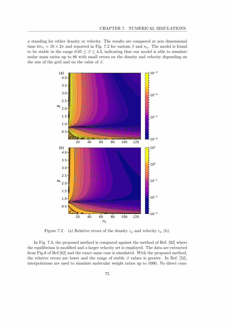
CHAPTER 7. NUMERICAL SIMULATIONS
ϕ standing for either density or velocity. The results are compared at non dimensionaltime ktce = 10 × 2π and reported in Fig. 7.2 for various β and nx. The model is foundto be stable in the range 0.05 ≤ β ≤ 4.3, indicating that our model is able to simulatemolar mass ratios up to 86 with small errors on the density and velocity depending onthe size of the grid and on the value of β.
20 40 60 80 100 120
0.5
1.0
1.5
2.0
2.5
3.0
3.5
4.0(a)
10 6
10 5
10 4
10 3
20 40 60 80 100 120nx
0.5
1.0
1.5
2.0
2.5
3.0
3.5
4.0(b)
10 3
10 2
10 1
100
101
Figure 7.2 – (a) Relative errors of the density ερ and velocity εu (b).
In Fig. 7.3, the proposed method is compared against the method of Ref. [62] wherethe equilibrium is modified and a larger velocity set is employed. The data are extractedfrom Fig.6 of Ref.[62] and the exact same case is simulated. With the proposed method,the relative errors are lower and the range of stable β values is greater. In Ref. [52],interpolations are used to simulate molecular weight ratios up to 1000. No direct com-
75

CHAPTER 7. NUMERICAL SIMULATIONS
parison is possible since no relative errors of the density and velocity are plotted, andboth of these errors have different orders of magnitude. Nonetheless, the present methodis easier to implement compare to interpolations which can be cumbersome to code in3D, especially on boundary nodes. The gain in CPU time is not the main reason of theuse of the proposed method. As a crude approximation, if we assume that the calculationof the density gradient has the same CPU cost as an interpolation of one distributionfunction, interpolations are 4 × (N − 1) times more expensive than using a force to alterthe equation of state in 2D where N is the number of species (one gradient calculationfor each physical dimension vs one interpolation for each distribution function). Forthe D3Q19 velocity set, interpolations are approximately 6 × (N − 1) more expensive.Anyway, the main CPU cost is as usual related to the collision operation.
0 1 2 3 4ratio of speed of sound [-]
10 5
rel.
dens
ity e
rror
[-]
D1Q3 Looije et al.D1Q5 Looije et al.present method
0 1 2 3 4ratio of speed of sound [-]
10 2
10 1
rel.
velo
city
erro
r v [
-]
D1Q3 Looije et al.D1Q5 Looije et al.present method
Figure 7.3 – Relative global errors for the decay of a density wave (nx = 256).
7.2 B- Equimolar counter-diffusion
In this test case, we study the mixing between two species of equal molecular massesfor which the mass transfer occurs only by diffusion, and governing equations are
∂tρm = D∇2ρm, for m = 1, 2. (7.7)
A particular solution of Eq. (7.7) is
ρm (x, t) = ρ0 + (−1)mδρ exp(−k2Dt) sin(kx). (7.8)
76

CHAPTER 7. NUMERICAL SIMULATIONS
We choose ρ0 = 1, δρ = 10−3, k = 2π/nx, and use a two-dimensional periodic domain(nx = 200, ny = 5). As an example, we plot in Fig. 7.4 the temporal evolution of ρ2 forD = 10−2 and τ = 1 for both species. Numerical results are indistinguishable from theanalytical solution Eq. (7.8).
0 50 100 150 200x
0.99900
0.99925
0.99950
0.99975
1.00000
1.00025
1.00050
1.00075
1.00100
2
t = 0t = 20000t = 40000t = 100000t = 200000t = 400000
Figure 7.4 – Evolution of ρ2 for τ = 1 and D = 10−2 at different iterations. Symbols andlines stand for simulation results and analytical solutions from Eq. (7.8), respectively.
For comparison, we have evaluated the error of the diffusion coefficient at variousD and relaxation times τ (which is assumed to be the same for the two species). Therelative error ||Dnum−D||/D is reported in Fig. 7.5 where Dnum is computed at x = nx/4by linear fit of Eq. (7.8) and D is set using Eq. (5.7). The numerical solution is in goodagreement with the theoretical results for D < 0.1 and for all relaxation times. We notethat the relative error in density, ερ as defined in Eq. (7.6), is three orders of magnitudesmaller than the relative errors of the diffusion coefficient. The figure shows a discrepancybetween the numerical and theoretical results for D > 0.1. Having kept constant the sizeof the domain for all D, this discrepancy is likely to be ascribed to a loss of spatial andtemporal resolution. Nonetheless the relative error of the diffusion coefficient is alwaysless than 0.4% for all τ . Different sizes of domain are used (not shown in the presentstudy) and we recover the classic second-order accuracy in space indicating that theforcing approach does not deteriorate the accuracy of the LBM algorithm.
7.3 C- Loschmidt’s tube
Having validated the ability of the method to simulate the decay of a single speciesdensity wave (at various different molar masses), and the counter-diffusion of species hav-
77

CHAPTER 7. NUMERICAL SIMULATIONS
10 6 10 5 10 4 10 3 10 2 10 1 100
Diffusion coefficient 10 5
10 4
10 3
Rela
tive
erro
r
= 0.6= 1= 2
Figure 7.5 – Relative errors of the diffusion coefficient.
ing equal molecular masses (at various diffusion coefficients), we simulate the Loschmidt’stube experiment [67]. The latter consists of the mixing of a ternary mixture of gaseshaving different molecular masses (argon, methane, and hydrogen). For such a process,a diffusion reversal is observed depending on the initial species composition [41]. Inparticular, we have considered two tubes of the same dimension filled with mixturesof different composition in the left and right tubes that are joined at the beginning ofthe experiment. In the experiment the left and right mean compositions are measuredin time during the mixing. In the experimental apparatus, the lengths of each tube isLref/2 ≈ 0.405 and the period of observation is approximately 1h. The initial molarfractions are given in Table 7.1, and the other physical parameters are summarized inTable 7.2.
tube xAr xCH4 xH2
left (0 < x < Lref/2) 0.509 − δ 2δ 0.491 − δright (Lref/2 < x < Lref ) 0.485 − δ 0.515 − δ 2δ
Table 7.1 – Initial molar fractions, in our simulation we take δ = 5 × 10⁻⁴ (in theexperiment, δ = 0).
The simulation is carried out on a domain size of (nx, ny) = (200, 25). Classicalbounce-back rules are used on the left and right boundaries, and periodic conditions areapplied on the top and bottom sides of the domain.
For computational purposes, we have rescaled the Maxwell-Stefan diffusion coeffi-
78

CHAPTER 7. NUMERICAL SIMULATIONS
Lref [m] 2√
1/60πp [Pa] 101325T [K] 307.15
m Ar CH4 H2Mm [g/mol] 39.948 16.0425 2.01588DAr m [mm2/s] − 21.57 83.35DCH4 m [mm2/s] 21.57 − 77.16DH2 m [mm2/s] 83.35 77.16 −µ0,m [µPa/s] 22.83 11.35 9.18
Table 7.2 – Physical parameters of the experiment.
cients by a factor 103, and the partial viscosities have been computed imposing the samespecies Schmidt numbers, which we define in terms of the pure viscosity as in the ex-periment. The aim of the rescaled factor is to increase the physical time step of thesimulation and obtain results with less computational resources. Indeed, a rather smalldomain is used but Loschmidt’s experiment lasts 1h. Let us define the conversion factorsbetween physical and LBM quantities for the length and the time:
Cl = lphy
lLBM, Ct = tphy
tLBM. (7.9)
In practice, we use the concept of lattice units where the LBM quantities are defined byspace step δxLBM = 1 and time step δtLBM = 1. In physical units, the total length of thetwo tubes is 0.8112m and the domain size is equal to nx = 200. This yields to a lengthconversion factor Cl = 0.8112/200 = 4.056 × 10⁻³m. The diffusion coefficients, in latticeunits, are given by:
DLBM = DphyCt
C2l
(7.10)
Assuming the same diffusion coefficients in both LBM and physical systems results inCt = [s]
[m2]C2l = 1.6451 × 10⁻⁵s. The experience lasts about 1h which is approximately
equivalent to 218 × 106 time steps in the LBM simulation. Using a rescaled factor andkeeping the Schmidt number constant in both systems reproduce the same physics ata lower computational cost. Note that simulations with different sizes of the domain(nx = 200, 2000) and rescaled factors (103, 102) leads to identical results subject to thestandard LBM discretisation errors.
Figure 7.6 reports the evolution of the mean molar fractions for the left and righttubes in non-dimensional time units t∗ = t×DArCH4/(Lref )2. The mean molar fractionsare in very good agreement with the experimental data. As expected, initially argondiffuses in the same direction of the concentration gradient contrary to the behaviorpredicted by using Fick’s law. This reverse diffusion occurs on a scale of approximately0.04 non-dimensional time units, and the concentration of argon attains a plateau inboth tubes in spite of the presence of large concentration gradients. The other speciesdo not exhibit such diffusion barrier. At later times, Fick’s like diffusion takes place. It
79

CHAPTER 7. NUMERICAL SIMULATIONS
is important to point out that this complex diffusion dynamics can only be recovered bythe Maxwell-Stephan equations [37].
0.000 0.025 0.050 0.075 0.100 0.125 0.150t *
0.0
0.1
0.2
0.3
0.4
0.5M
olar
frac
tion
Figure 7.6 – Comparison between simulation (lines) and experimental data (symbols)extracted from Ref. [68]. Molar fraction of argon, blue; molar fraction of methane,orange; molar fraction of hydrogen, green. Solid lines and filled symbols, left tube;dashed lines and unfilled symbols, right tube.
7.4 D- Opposed jets flow
The model is finally validated for a flow whose dynamics is dominated by a convection-diffusion competing mechanism. The test case that we investigate is the same proposedin Ref. [51], which consists of two opposed jets of quaternary mixtures of gases hav-ing different initial concentrations (see Fig. 7.7 and Table 7.3). The domain size is(nx, ny) = (200, 400) and the widths of the left and right incoming streams are the sameand equal to 0.4ny. At left and right boundaries, equilibrium is assumed for the distri-bution functions, and the velocity is set equal to zero. For the left and right incomingstreams, we assume that all species velocities are respectively equal to UL = U0 andUR = −0.936U0 (as inferred from Fig. 3 of Ref. [51]), and we chose U0 = 0.04. At thetop and bottom boundaries, the outer incoming distribution functions are extrapolatedfrom the interior. The transport coefficients are evaluated by means of Eqs (6.40-6.43) atatmospheric pressure and temperature T = 300K. The species kinetic constants neededto evaluate the Ω-integrals are given in Table 7.4.
Figure 7.8 shows the distributions of the molar fractions and the mixture mass ve-
80

CHAPTER 7. NUMERICAL SIMULATIONS
0 100 200x
0
50
100
150
200
250
300
350
400y
0.00
0.01
0.02
0.03
0.04
0.05
Figure 7.7 – Molar fraction and velocity streamline plot of H2O.
locity at the symmetry plane (y = ny/2) and at steady state. The results are in closeagreement with Ref. [51] where the CHEMKIN package is used to calculate the transportcoefficients and mixture-averaged diffusion coefficients are employed for each species.This is however only correct asymptotically when there is either only one bulk com-ponent and trace species, or when all species but one have nearly the same diffusionvelocities, or when all the diffusion coefficients are the same. Despite using a simplifyingmixture-average diffusion, the results are similar since the multi-components diffusioneffects, which can not be captured with this assumption, are not significant. In addition,these transitory complex diffusion phenomena as in the case of the Loschmidt’s tubeexperiment (Sec. 7.3) would not be visible on this steady state comparison. Figure 7.8confirms that our model correctly predicts the dynamics of the flow characterized by acompeting convection-diffusion mechanism.
81
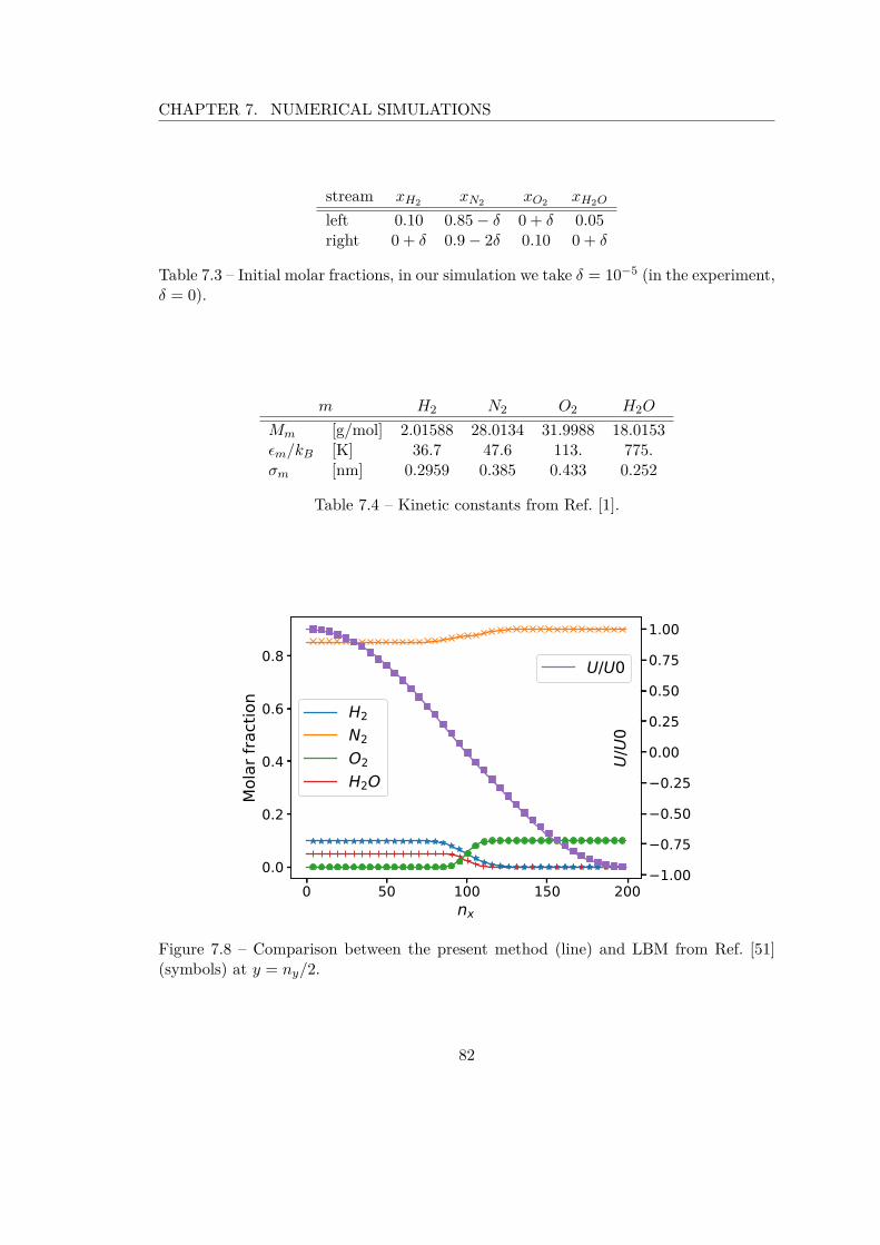
CHAPTER 7. NUMERICAL SIMULATIONS
stream xH2 xN2 xO2 xH2O
left 0.10 0.85 − δ 0 + δ 0.05right 0 + δ 0.9 − 2δ 0.10 0 + δ
Table 7.3 – Initial molar fractions, in our simulation we take δ = 10−5 (in the experiment,δ = 0).
m H2 N2 O2 H2O
Mm [g/mol] 2.01588 28.0134 31.9988 18.0153ϵm/kB [K] 36.7 47.6 113. 775.σm [nm] 0.2959 0.385 0.433 0.252
Table 7.4 – Kinetic constants from Ref. [1].
0 50 100 150 200nx
0.0
0.2
0.4
0.6
0.8
Mol
ar fr
actio
n
H2N2O2H2O
1.00
0.75
0.50
0.25
0.00
0.25
0.50
0.75
1.00U
/U0
U/U0
Figure 7.8 – Comparison between the present method (line) and LBM from Ref. [51](symbols) at y = ny/2.
82
Chapter 8
Synthesis
In the present chapter, we derive, explain and validate a lattice Boltzmann modelfor miscible gases. We show that the mixing dynamics of multi-species mixtures can besimulated by a forcing term in the lattice Boltzmann algorithm [Eq. (5.7)] and the addi-tion of a body force to account for species having different molecular masses [Eq. (5.13)].Furthermore, the model also relies on the use of transport coefficients that are calculatedby an approximation of the relations obtained from kinetic theory [Eq. (6.40)].
The model is validated against analytical, experimental, and numerical results avail-able in the literature. We have shown that the model can accurately simulate the decayof a density wave for a variety of pseudo speed of sound corresponding to molar massratios up to 86. The model adequately predicts the diffusion process in binary andternary mixtures of gases as shown in the case of the equimolar counter-diffusion andLoschmidt’s tube experiment. Complex diffusion phenomena such as reverse diffusionoccur in ternary mixtures. These phenomena are well observed in our model, and thedynamics predicted by the Maxwell-Stefan equations is correctly recovered. The presentmodel also adequately predicts the dynamics of flows where convection and diffusioncompete as in the case of two opposed jets of mixtures.
Finally, one of the advantages of the forcing approach is the easiness of implemen-tation. Since the collision is not altered, the method that we propose can easily beintroduced in any other lattice Boltzmann algorithm in order to take into account com-plex diffusion among species. Upcoming applications of the present model focus oninstabilities resulting from the transient mixing dynamics in porous media.
83


Part III
Simulation of the viscousfingering by the lattice
Boltzmann method
85


9 Viscous fingering instability 89
10 Porous medium in LBM 9310.1 Gray lattice Boltzmann . . . . . . . . . . . . . . . . . . . . . . . . . . . . 9310.2 Brinkman drag force . . . . . . . . . . . . . . . . . . . . . . . . . . . . . . 94
11 Numerical simulations 9511.1 Darcy’s law . . . . . . . . . . . . . . . . . . . . . . . . . . . . . . . . . . . 9511.2 Viscous fingering . . . . . . . . . . . . . . . . . . . . . . . . . . . . . . . . 9511.3 Viscous fingering caused by reverse diffusion . . . . . . . . . . . . . . . . . 106
12 Synthesis 111
87

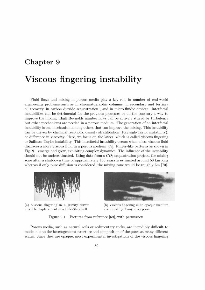
Chapter 9
Viscous fingering instability
Fluid flows and mixing in porous media play a key role in number of real-worldengineering problems such as in chromatographic columns, in secondary and tertiaryoil recovery, in carbon dioxide sequestration , and in micro-fluidic devices. Interfacialinstabilities can be detrimental for the previous processes or on the contrary a way toimprove the mixing. High Reynolds number flows can be actively stirred by turbulencebut other mechanisms are needed in a porous medium. The generation of an interfacialinstability is one mechanism among others that can improve the mixing. This instabilitycan be driven by chemical reactions, density stratification (Rayleigh-Taylor instability),or difference in viscosity. Here, we focus on the latter, which is called viscous fingeringor Saffman-Taylor instability. This interfacial instability occurs when a less viscous fluiddisplaces a more viscous fluid in a porous medium [69]. Finger-like patterns as shown inFig. 9.1 emerge and grow, exhibiting complex dynamics. The influence of the instabilityshould not be underestimated. Using data from a CO2 sequestration project, the mixingzone after a shutdown time of approximately 150 years is estimated around 50 km longwhereas if only pure diffusion is considered, the mixing zone would be roughly 5m [70].
(a) Viscous fingering in a gravity drivenmiscible displacement in a Hele-Shaw cell.
(b) Viscous fingering in an opaque mediumvisualized by X-ray absorption.
Figure 9.1 – Pictures from reference [69], with permission.
Porous media, such as natural soils or sedimentary rocks, are incredibly difficult tomodel due to the heterogeneous structure and composition of the pores at many differentscales. Since they are opaque, most experimental investigations of the viscous fingering
89

CHAPTER 9. VISCOUS FINGERING INSTABILITY
phenomena are carried out on Hele-Shaw cells. A Hele-Shaw cell is composed of twoparallel plates with a small gap. This flow configuration mimic the drag induced bya porous medium when the gap is small enough. From a numerical point of view, thesimulation of a large-scale flow at the pore scale is often impractical because of longCPU time and excessive memory consumption. Hence, a volume average approach isusually used to overcome these difficulties. In this case, Darcy or Darcy-Brinkman semi-empirical equations are solved and porosity, permeability, and other measurements aredefined. In the case of a single fluid, the Brinkman equation adds a drag force to theStokes equations,
∇p = − µ
Ku + ∇ ·
[µe
(∇u + (∇u)T
)](9.1)
where p is the pressure, K is the permeability of the medium, u is the fluid velocity, andµe is the effective viscosity which may not be equal the fluid viscosity. The Brinkmanequations are a convenient transition model between Darcy regime (K ≪ L2µ/µe, withL the macroscopic characteristic length) and Stokes regimes (K ≫ L2µ/µe). In a Hele-Shaw cell, one can show that the flow is also governed by Darcy’s law with an equivalentpermeability of b2/12 in the limit of low Reynolds number flow and b/L → 0, where b isthe small gap width. It is to be noted that the dynamics of the viscous fingering is mainlygoverned by the Darcy equation [69] therefore Stokes’ term is not of primary importanceand the effective viscosity is taken equal to the fluid viscosity unless otherwise stated.Indeed, most of the literature (see previous and next references) only considers Darcy’sequations. The latter equations correctly described flows in Hele-Shaw cells and in simpleporous media whereas Darcy-Brinkman’s equations are often used as a transition modelbetween porous flow and Stokes flow such as in the case of fractured porous media.
Now we consider a homogeneous porous medium and a zone where the viscosityvaries greatly. Under suitable assumptions, the flow follows a one-dimensional Darcy’slaw and the pressure differential from both sides of the fictional interface as a result ofa virtual displacement δx reads
δp = (pleft − pright) = (µright − µleft)U/Kδx (9.2)
If the net total pressure δp is positive, then any small displacement will amplify, resultingin an instability. From this simple argument, the instability mechanism is driven by theviscosity difference on either side of the interface. If the displaced fluid is more viscousthan the displacing (µright > µleft) then the configuration is unstable, in the contrary(µright < µleft) any small interface perturbation will be damped and the configurationis stable.
Since the pioneer work of Hill [71] in 1952 and Saffman and Taylor [72] in 1958,extensive investigations has been performed on both immiscible and miscible fluids. Adistinctive characteristic of miscible fluids is the lack of a sharp interface and surfacetension. Mixing produces changes in the fluid since the properties of the mixture varycontinuously while diffusion occurs. Usually, the viscous fingering is modeled by usingDarcy’s law and a scalar transport equation for the concentration. A relation betweenthe viscosity and the concentration of the components must be defined. Most articles
90

CHAPTER 9. VISCOUS FINGERING INSTABILITY
follow the standard literature rather than physical rigor and assume an exponentialdependence.
Studies of the viscous fingering instability can be divided into two categories: linearstability analyses and non-linear simulations. The linear stability analysis is a classicaltool to study the evolution of small perturbations that leads to the instability. Themain mathematical challenge of the miscible viscous fingering is due to the unsteadybase (i.e. unperturbed) state caused by diffusion. In practice, the quasi-steady-stateapproximation is employed and the linear stability analysis is applied on a frozen basestate at successive frozen times [73, 74]. Other methods such as initial value problem ornon-modal analysis (transient growth analysis) are possible. Excluding very short times,the different approaches are in good agreement [73, 75]. As its name implies, the linearstability analysis is restricted to early times. As the perturbation develops, non-linearinteractions occur and the linearized equations are no longer valid. This leads to thesecond category: non-linear simulations where no approximation is made, thus the fulllife cycle of fingers, from onset to shutdown, can be studied. In this case, equationsare solved with a stream-function formulation using spectral method [73, 74, 76, 77] orfinite-difference method [78, 70]. The former is very efficient whereas the latter can benumerically stable for any viscosity ratios.
Lattice Boltzmann method was also used to study the viscous fingering phenomenon.In 1992, Holme and Rothman [79] propose a LBM for miscible binary fluids where onedistribution function models an advection-diffusion equation and a second distributionfunction is employed for the mixture density and momentum balance equations. Then,they simulate the viscous fingering instability using their miscible model with a variablemixture viscosity and a drag force that mimics the effect of a porous medium. With asimilar miscible LBM approach, Rokotomalala, Salin, and Watzky [80] study the miscibledisplacement of two fluids with different viscosities between two parallel plates. Inthe absence of porous medium, a single finger may appear depending on the diffusionand the viscosity contrast. This can be seen as a limit case of the viscous fingeringinstability. Contrary to the previous model where an advection-diffusion equation forthe concentration is solved, a more natural approach in order to deal with diffusion inthe frame of the lattice Boltzmann method is the use of an inter-molecular friction force.Indeed, the distribution function for the diffusion equation lost its molecular meaningand is no longer associated with the physical description of a species, i.e., collisions ofmolecules. More specifically, the diffusion equation is postulated and a kinetic schemeis tailored so as to solve it. Here, neither transport equation for the concentration, norDarcy equation with exponential viscosity dependency are solved. Each species dynamicis governed by its own kinetic equation [Eq. (5.1)] where diffusion is taken into account bymeans of an inter-molecular force and the viscosity of species stemmed from the kinetictheory of gases [Eq. (6.40)]. Adopting a lattice Boltzmann approach, we investigatetwo strategies to mimic the porous medium effects: the gray lattice Boltzmann modelassuming a partial reflection condition and the Brinkman force model adding a dragforce.
Viscous fingering is a fascinating and a pertinent phenomenon to showcase the possi-
91

CHAPTER 9. VISCOUS FINGERING INSTABILITY
bilities of our miscible model. This instability exhibits complex dynamics depending onboth molecular diffusion and viscosity namely inter-molecular friction forces and partialviscosities in our case. A few questions arise. Can we simulate the viscous fingeringinstability with the present model? What is the influence of the viscosity law? How theinstability is modified when multi-component effects take place in ternary mixtures?
92

Chapter 10
Porous medium in the latticeBoltzmann method
In this chapter, we briefly present how to model the porous medium within a lat-tice Boltzmann framework. As described earlier, we seek for an average view of theporous medium and the equivalent target macroscopic equation is Darcy (-Brinkman) ’sequation.
10.1 Gray lattice Boltzmann
Taking the advantage of the mesoscopic view of the lattice Boltzmann method, aporous medium can be modeled by different means. We first present the so-called graylattice Boltzmann (GLBM) scheme where a special condition is applied on the wholedomain: in each cell during the streaming step, the distribution functions are bouncedback with a certain amount. Various schemes are proposed in the literature. In Ref. [81],the local pre-collision distribution functions are reflected whereas in Ref. [82], the localpost-collision distribution functions are taken as reflected distribution functions. Yoshidaand Hayashi [83] also suggest a gray lattice Boltzmann model based on Ref. [84] but theneighboring post-collision distribution functions are reflected. Despite some differences,all the previous gray lattice Boltzmann schemes [81, 82, 83] recover the Darcy-Brinkmanequation [85]. In this study, the use of the model proposed in Ref. [83] is motivated bytwo main reasons. First, a redefinition of the macroscopic velocity is not required inthis latter scheme. This redefinition would lead to complicated expressions especiallyon the boundary nodes since in the present approach, velocity and forces are coupled[Eqs. (5.6-5.7)]. Furthermore, the classical bounce-back boundary condition is obtainedas a limit expression. If we use the notation Γm
α to substitute for the right-hand side ofEq. (5.1) (post-collision part), the following gray lattice Boltzmann scheme is obtained,
fmα (x + eαδt, t+ δt) = (1 − θm)Γm
α (x, t) + θmΓmα (x + eαδt, t) , (10.1)
93

CHAPTER 10. POROUS MEDIUM IN LBM
where Γmα (x + eαδt, t) are the post-collision distribution functions from the opposite
direction of α velocity located at the neighboring node and θm is the amount of reflection.The principle of the algorithm is depicted in Fig. 10.1
Figure 10.1 – Sketch of the gray lattice Boltzmann algorithm. The resulting streamingstep in GLBM is composed of a fraction of the standard propagated distribution functionand a reflected part from the opposite lattice direction.
When θm = 0, the usual streaming step occurs and θm = 1 is similar to the classicalbounce-back (no-slip) condition. For 0 < θm < 1, the scheme mimics the dynamics ofa porous medium and this approach should be related to a subgrid model for porousmedium. The parameter θm depends on the viscosity of the fluid and the permeabilityof the considered porous medium and the following relation can be obtained [83, 85]
µm
Kρm= 2θm
(1 − θm)δt(10.2)
Here, θ is defined on the link between nodes instead of being a node based value. Ineach direction α of the lattice, θ is computed by the means of an interpolation betweenthe two nodes. This ensures that the mass is conserved strictly by the scheme.
10.2 Brinkman drag forceIn the second approach, referred as Brinkman force (BF) model, the porous medium
resistance is included explicitly through a drag force in the lattice Boltzmann equation,e.g. [80, 86, 87, 88, 89, 90]. Here, we follow a similar approach and the forcing term iswritten as
Fporous,m = −µm
Kum. (10.3)
Compared to the gray lattice Boltzmann, this strategy is local and has a negligiblecomputational cost since we already implement a source term because of the inter-molecular friction forces. As mentioned in Refs.[23, 24, 91], the numerical permeabilitydepends lightly on the viscosity for both Brinkman force and gray lattice Boltzmannmodels. This nonphysical variation can be alleviated by keeping the so-called magicnumber Λ constant (see [22, 23, 24, 86, 91]). We use the multiple relaxation times(MRT) collision model with Λ = 3/16 corresponding to sq = 82−1/τm
8−1/τm.
94

Chapter 11
Numerical simulations
11.1 Darcy’s law
In order to show that Darcy’s law is recovered by both of the proposed schemes, a flowcomposed of two identical species (m = 1, 2 and βm = 1) through a homogeneous porousmedium is simulated. Domain size is set to (nx = 101, ny = 20). Periodic conditionsare applied on top and bottom of the domain and a constant velocity profile (ux,m =U, uy,m = 0) is imposed at left and right side of the domain via the non-equilibriumbounce-back. Distribution functions are initialized at their equilibrium values with anuniform initial density field ρ1 = ρ2. Simulation is stopped when steady state is achieved.In Figure 11.1, the pressure drop between the left and right side of the domain is plottedagainst the horizontal inlet velocity. Both gray lattice Boltzmann and Brinkman forcemodels give equivalent results and show the expected Darcy behavior of the simulatedsystem.
This first result shows that both porous modeling strategies are able to accuratelyreproduce the standard behaviour of a porous medium for different values of K.
11.2 Viscous fingering
The viscous fingering instability occurs when a less viscous fluid invade a more viscousfluid. In the case of miscible fluids, if the interface between fluids is sharp enough, finger-like patterns emerge and grow, exhibiting complex dynamics. Following the literature,dimensionless parameters are defined such as the log-viscosity ratio, the Péclet number(ratio of the advective transport rate and the diffusive transport rate), and the Darcynumber:
R = ln(µ0,2µ0,1
), Pe = ULref
D12, Da = K
Lref2 , (11.1)
where U is the injected velocity and Lref is the reference length. Here following Ref. [74],the characteristic scales are based on the convective length: Lref is taken as the height ofthe domain and the reference time is tref = Lref/U . If R < 0, the invading fluid is more
95

CHAPTER 11. NUMERICAL SIMULATIONS
10−4 10−3 10−2 10−1
um
10−7
10−6
10−5
10−4
10−3
−∇p m
K = 10
K = 100
K = 1000
Figure 11.1 – Pressure drop according to the velocity for different permeability at fixedviscosity µ0,m = 2 × 10⁻¹ lu. Values are given in lattice units (lu). Squares and starsstand for numerical results obtained respectively with the gray lattice Boltzmann andthe Brinkman force schemes. Lines are the analytical solution −∇pm = µm/KU .
viscous than the resting fluid, and the interface is always stable. On the other hand, ifR > 0, the invading fluid is less viscous than the resting fluid, and the interface betweenthe two fluids may be unstable. The number of fingers increases with both the Pécletnumber and the ratio R. We recall that the relation between the pure viscosity and thespecies is given by Eq. (6.40). The influence of different parameters on the instability isstudied. First, we present the numerical configuration employed to simulate the viscousfingering instability. The early times of the instability are compared with results fromlinear stability analysis and for intermediate times, we focus the evolution of the mixinglength induced by the fingering. Effects of the Péclet number, and the porous model(gray lattice Boltzmann or Brinkman force models) are highlighted.
11.2.1 Numerical configuration
In the following simulations, the fluid consists of two species having equal molarmasses (βm = 1 m = 1, 2). The resting mixture is composed of molar fractions x1 = 0.1and x2 = 0.9 and these are swapped for the injected mixture (x1 = 0.9, x2 = 0.1). Thedomain considered is two-dimensional and we impose periodicity at the top and bottomboundaries. At the left and right boundaries, a constant velocity condition equal to Uis applied for both species. Each simulation is initialized by an almost sharp interface
96
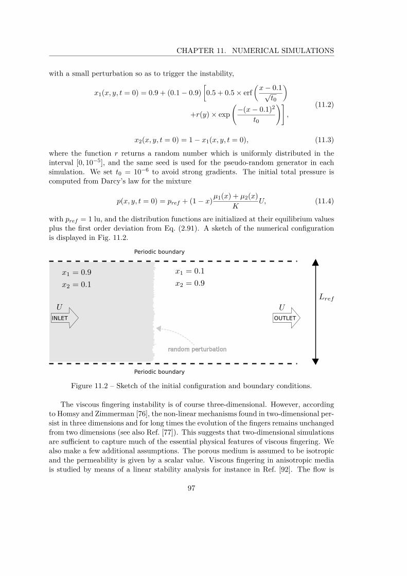
CHAPTER 11. NUMERICAL SIMULATIONS
with a small perturbation so as to trigger the instability,
x1(x, y, t = 0) = 0.9 + (0.1 − 0.9)[0.5 + 0.5 × erf
(x− 0.1√
t0
)+r(y) × exp
(−(x− 0.1)2
t0
)],
(11.2)
x2(x, y, t = 0) = 1 − x1(x, y, t = 0), (11.3)
where the function r returns a random number which is uniformly distributed in theinterval [0, 10−5], and the same seed is used for the pseudo-random generator in eachsimulation. We set t0 = 10−6 to avoid strong gradients. The initial total pressure iscomputed from Darcy’s law for the mixture
p(x, y, t = 0) = pref + (1 − x)µ1(x) + µ2(x)K
U, (11.4)
with pref = 1 lu, and the distribution functions are initialized at their equilibrium valuesplus the first order deviation from Eq. (2.91). A sketch of the numerical configurationis displayed in Fig. 11.2.
Figure 11.2 – Sketch of the initial configuration and boundary conditions.
The viscous fingering instability is of course three-dimensional. However, accordingto Homsy and Zimmerman [76], the non-linear mechanisms found in two-dimensional per-sist in three dimensions and for long times the evolution of the fingers remains unchangedfrom two dimensions (see also Ref. [77]). This suggests that two-dimensional simulationsare sufficient to capture much of the essential physical features of viscous fingering. Wealso make a few additional assumptions. The porous medium is assumed to be isotropicand the permeability is given by a scalar value. Viscous fingering in anisotropic mediais studied by means of a linear stability analysis for instance in Ref. [92]. The flow is
97

CHAPTER 11. NUMERICAL SIMULATIONS
more stabilized when the ratio of longitudinal to transverse anisotropic permeability isincreased. Similarly, we only consider molecular diffusion and do not take into accountthe (anisotropic) dispersion caused in the flow at the pore scale since a general Taylordispersion model is not known. One can note that the previous authors find from thelinear stability analysis that the flow is more stable when the ratio of longitudinal totransverse anisotropic dispersion is decreased. With these assumptions, we will be ableto compare our results with the classical literature.
A fine spatial discretization is required in order to resolve accurately all the lengthscales of the instability, especially at high Péclet numbers. Preliminary simulations areperformed to find the appropriate grid spacing. Three square grids are considered withdifferent resolutions corresponding to ny = 1000, 2000, 4000 where Lref is kept constant.The initial random perturbation is based on the grid where ny = 1000 and interpolationsare used for higher resolutions. Otherwise stated, we set
R = 3 (µ0,2 ≈ 20µ0,1), Pe = 5000, Da = 6.25 × 10⁻⁸, (11.5)
Re0,1 = ULrefρref
µ0,1= 10, Ma = U
cs=
√3 × 10⁻³. (11.6)
With this specific value of Mach number, the inlet velocity is equal to 10−3 lu. Thiscorresponds to a low Reynolds flow in the Darcy regime at moderate Péclet number andviscosity ratio. We recall that two different system of units are defined. On one handthere is the lattice unit system where the time and space step are equal to one, andon the other hand the physical system. Nonetheless, all the dimensionless numbers areequal for either system of units.
For each resolution at different times, we carry out a fast Fourier transform (FFT) ofthe fingers. In particular, we take a slice of the domain where the mean molar fractionalong the transverse direction is included in the interval [0.11, 0.89]. Afterwards, weaverage along the longitudinal direction and apply a FFT to obtain the spectrum of theinterface deformation according to the y-axis spatial frequency as plotted in Fig.11.3.Results for different resolutions are compared at the same non-dimensional time
t∗ = t
tref= tU
Lref. (11.7)
For short times, the lowest resolution corresponding to ny = 1000 is not able toresolve the high frequencies of the instability. As the time progresses, larger structuresappear and are captured by three resolutions, but for ny = 1000 the amplitude of thefingers is slightly over-predicted. Resolutions corresponding to ny = 2000 and ny =4000 give equivalent results suggested that the main length scales of the instability aresufficiently well resolved. Nonetheless, we point out that global quantities such as themean molar fraction or the mixing length are less sensitive to the resolution and canbe adequately captured even with a very coarse grid. Theses results are in agreementwith the linear stability analysis of a steep initial profile made in Ref. [74]. At initialtime t = 0, an analytical dispersion curve can be obtained and the cutoff wave numberis found equal to RPe/4 = 3750 corresponding to a wave length of 0.0016. With a
98
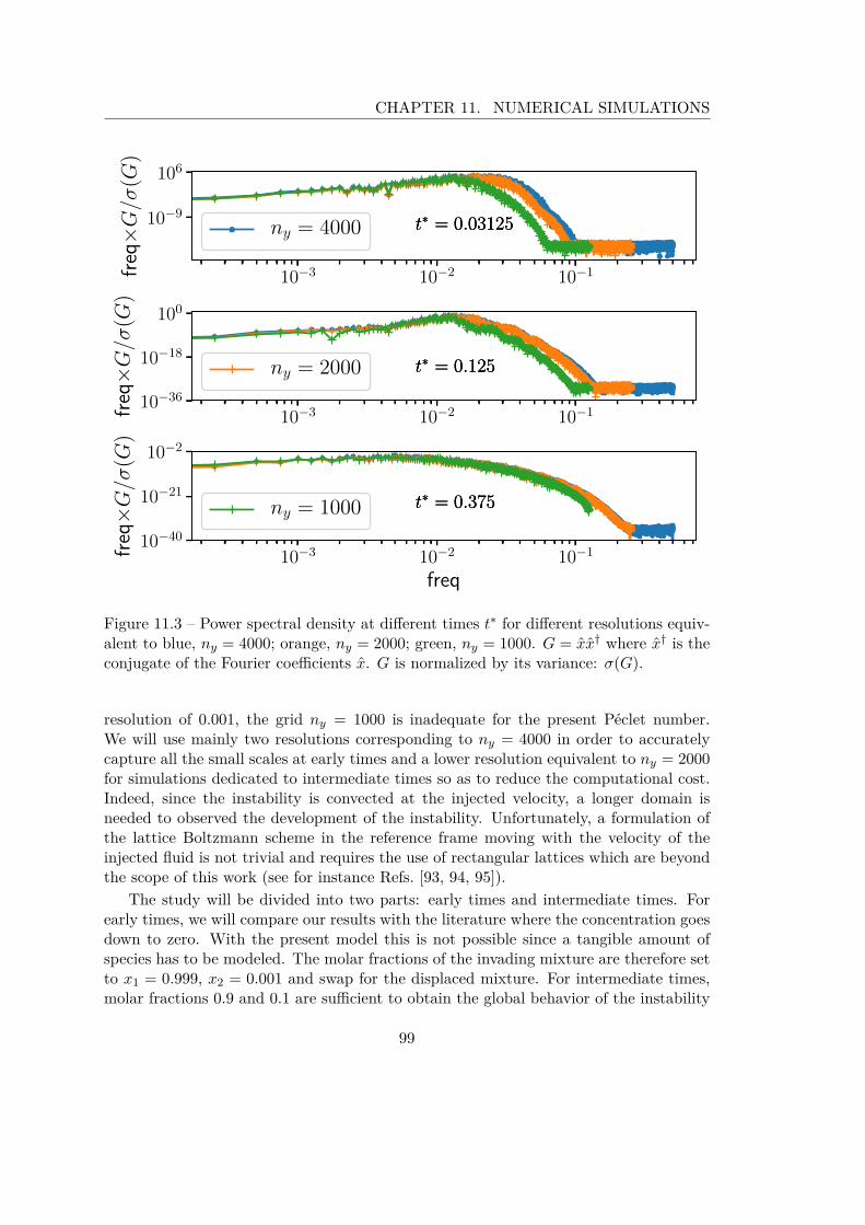
CHAPTER 11. NUMERICAL SIMULATIONS
10−3 10−2 10−1
10−9
106
freq×G/σ
(G)
t∗ = 0.03125t∗ = 0.03125t∗ = 0.03125ny = 4000
10−3 10−2 10−110−36
10−18
100
freq×G/σ
(G)
t∗ = 0.125t∗ = 0.125t∗ = 0.125ny = 2000
10−3 10−2 10−1
freq
10−40
10−21
10−2
freq×G/σ
(G)
t∗ = 0.375t∗ = 0.375t∗ = 0.375ny = 1000
Figure 11.3 – Power spectral density at different times t∗ for different resolutions equiv-alent to blue, ny = 4000; orange, ny = 2000; green, ny = 1000. G = xx† where x† is theconjugate of the Fourier coefficients x. G is normalized by its variance: σ(G).
resolution of 0.001, the grid ny = 1000 is inadequate for the present Péclet number.We will use mainly two resolutions corresponding to ny = 4000 in order to accuratelycapture all the small scales at early times and a lower resolution equivalent to ny = 2000for simulations dedicated to intermediate times so as to reduce the computational cost.Indeed, since the instability is convected at the injected velocity, a longer domain isneeded to observed the development of the instability. Unfortunately, a formulation ofthe lattice Boltzmann scheme in the reference frame moving with the velocity of theinjected fluid is not trivial and requires the use of rectangular lattices which are beyondthe scope of this work (see for instance Refs. [93, 94, 95]).
The study will be divided into two parts: early times and intermediate times. Forearly times, we will compare our results with the literature where the concentration goesdown to zero. With the present model this is not possible since a tangible amount ofspecies has to be modeled. The molar fractions of the invading mixture are therefore setto x1 = 0.999, x2 = 0.001 and swap for the displaced mixture. For intermediate times,molar fractions 0.9 and 0.1 are sufficient to obtain the global behavior of the instability
99

CHAPTER 11. NUMERICAL SIMULATIONS
with a coarse grid.
11.2.2 Early times
At early times, the interface between the two mixtures spreads because of diffusionand start to deform. At the very beginning, the flow is linearly unstable and perturba-tions grow exponentially. The onset of fingers is explored by many authors using linearstability analysis [69, 73, 74, 75, 70, 92]. The Darcy’s equation, the continuity equa-tion, and the transport equation for the concentration are linearized and a dispersionequation is solved so as to compute the growth rate of the perturbation. An analyticalsolution is only known for the initial time and numerical methods have then to be em-ployed. Linear stability analysis can also be directly performed in the lattice Boltzmannframework (see. [96, 97]) however this approach is still in its infancy and is only appliedto simple single fluid flows. In this study we carry out non-linear simulations with theaforementioned lattice Boltzmann model and compute the growth rate of the perturba-tion a posteriori. This present approach has the advantage to avoid the development ofanother tool and is valid for the whole instability including the non-linear stage. Themolar fractions can be decomposed into a base state x0
m and a perturbative componentx′
m,xm(x, t) = x0
m(x, t) + x′m(x, t). (11.8)
We assume that the perturbation can be expressed in the form of
x′m(x, t) = x′
m(x) exp (σt) (11.9)
where σ is the growth rate of the perturbation. The dispersion curves are obtained byapplying a fast Fourier transform (FFT):
x′m(x, t) = x0
m(x, t) − xm(x, t) (11.10)x(x, k, t) = FFTy
(x′
m(x, t))
(11.11)
a(k, t) = ||x(x, k, t)||2 =√∫
x · x†dx (11.12)
σ(k, t) = d ln (a(k, t))dt
(11.13)
where x† is the complex conjugate of x, k is the wave number and we choose a timestep sufficiently small such as the growth rate can be considered as constant betweentwo derivation steps. a represents a measure in the Fourier space of the amplification ofthe perturbed molar fraction. Only relevant growth rates are of interest, consequentlythe growth rate of perturbations whose amplitude is less than 10−4 × max∀k(a(k, t)) isfiltered out. The perturbative components are computed by subtracting the componentsfrom the non-linear perturbed solution to the components from the base state. This basestate is obtained by simulating the exact same conditions with no initial perturbation.
100
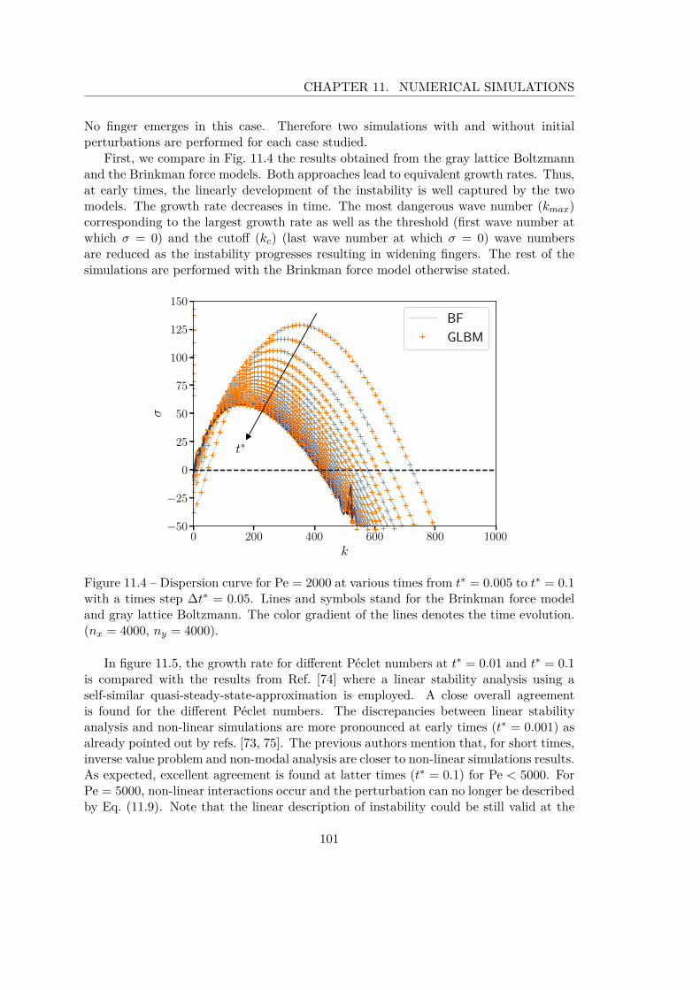
CHAPTER 11. NUMERICAL SIMULATIONS
No finger emerges in this case. Therefore two simulations with and without initialperturbations are performed for each case studied.
First, we compare in Fig. 11.4 the results obtained from the gray lattice Boltzmannand the Brinkman force models. Both approaches lead to equivalent growth rates. Thus,at early times, the linearly development of the instability is well captured by the twomodels. The growth rate decreases in time. The most dangerous wave number (kmax)corresponding to the largest growth rate as well as the threshold (first wave number atwhich σ = 0) and the cutoff (kc) (last wave number at which σ = 0) wave numbersare reduced as the instability progresses resulting in widening fingers. The rest of thesimulations are performed with the Brinkman force model otherwise stated.
0 200 400 600 800 1000
k
−50
−25
0
25
50
75
100
125
150
σ
t∗
BF
GLBM
Figure 11.4 – Dispersion curve for Pe = 2000 at various times from t∗ = 0.005 to t∗ = 0.1with a times step ∆t∗ = 0.05. Lines and symbols stand for the Brinkman force modeland gray lattice Boltzmann. The color gradient of the lines denotes the time evolution.(nx = 4000, ny = 4000).
In figure 11.5, the growth rate for different Péclet numbers at t∗ = 0.01 and t∗ = 0.1is compared with the results from Ref. [74] where a linear stability analysis using aself-similar quasi-steady-state-approximation is employed. A close overall agreementis found for the different Péclet numbers. The discrepancies between linear stabilityanalysis and non-linear simulations are more pronounced at early times (t∗ = 0.001) asalready pointed out by refs. [73, 75]. The previous authors mention that, for short times,inverse value problem and non-modal analysis are closer to non-linear simulations results.As expected, excellent agreement is found at latter times (t∗ = 0.1) for Pe < 5000. ForPe = 5000, non-linear interactions occur and the perturbation can no longer be describedby Eq. (11.9). Note that the linear description of instability could be still valid at the
101

CHAPTER 11. NUMERICAL SIMULATIONS
time t∗ = 0.1 if the flow is initially perturbed by only one wave number instead ofbeing excited on the whole spectrum. This more accurate strategy required to runa simulation (two precisely for the perturbed and non-perturbed cases) for each wavenumber of interest. This becomes rapidly unpractical if one wants to study the timeevolution of the instability as the relevant wave numbers where σ > 0 depends on timeand shift toward smaller wave numbers as time progresses.
0 200 400 600 800 1000 1200 1400
k
−50
0
50
100
150
200
250
σ
t∗ = 0.01
0 200 400 600 800 1000
k
−50
0
50
100
150
200
250
σ
t∗ = 0.1
Pe = 5000 Pe = 2000 Pe = 1000 Pe = 500
Figure 11.5 – Dispersion curves for R = 3 at t∗ = 0.01, 0.1 with different Péclet values.Lines stand for the simulation and the symbols are data obtained by a linear stabilityanalysis from Ref. [74]. (nx = 4000, ny = 4000).
Diffusion acts as a stabilization factor by smoothing perturbations and heading toan homogeneous mixture. Hence, as shown in Fig. 11.5, the instability is more dominantat higher Péclet numbers. A lower fluid dispersion expands the range of unstable wavenumbers and increases the growth rate. The cutoff wave number increases with the Pécletnumber whereas it has a very limited influence on the threshold wave number. This canbe easily seen on neutral stability curves (contours of σ = 0) plotted in Fig. 11.6. Thedifferences from the bell-shaped curve is due to the non-linear interactions. The areaabove the neutral curve defines the region of instability. As described earlier, this regionincreases with the Péclet number. The minimum (t∗crit, kcrit) on the neutral curves is thelimit below the perturbation is stable. It is interesting to note that we can also definea critical Péclet number Pecrit and its value depends on the time. For Pe = 500 andPe = 1000, the flow is initially stable then becomes unstable at latter times whereasfor Pe = 5000 at t∗ = 0 the flow seems already unstable. For very short times, thegrowth of the interface caused by large diffusion (low Péclet numbers) surpasses theexponential growth of the perturbation. This also implies that, as expected, there isa minimal critical Péclet number such as the flow is always stable when the diffusionis large enough. Nonetheless, more simulations with smaller time steps and variousPéclet numbers should be performed to quantity this phenomenon and dismiss numericaltransient artifacts especially for large Péclet numbers. The time variations of the most
102

CHAPTER 11. NUMERICAL SIMULATIONS
dangerous wave number and respectively the cutoff wave number follows the same trend.In Appendix D.1, the most dangerous and the cutoff wave numbers are plotted in alogarithm scale according to the time and straight lines are obtained for t∗ > 0.01. Fora log viscosity ratio R = 3, the most dangerous wave number decreases rapidly thenslower as kmax ∼ t∗−0.26 compared to the cutoff wave number where kc ∼ t∗−0.36. Wecan also compute approximately the change with the Péclet number, kc ∼ Pe0.59 andkmax ∼ Pe0.70. As seen in fig. 11.6, a higher Péclet number expands considerably therange of unstable wave numbers. High Péclet number flows are difficult to simulatebecause of limitations required on time and space resolutions if one wants to resolve allthe length scales of the instability.
100 101 102 103
k
0.00
0.02
0.04
0.06
0.08
0.10
t∗
Pe = 5000
Pe = 2000
Pe = 1000
Pe = 500
Figure 11.6 – Neutral stability curves (σ = 0) for different Péclet numbers at R = 3according to the time and the wave number. Dashed lines represent the most dangerouswave number kmax. For t∗ > 0.035 and Pe = 5000, non-linear interactions take placeand the most dangerous wave number is not plotted. (nx = 4000, ny = 4000).
11.2.3 Intermediate times
Figure 11.7 shows a sequence of snapshots of a simulation performed with the Brinkmanforce model at R = 3, Pe = 2000. At early times (t∗ ≤ 0.1), the sharp interface diffusesand begins to deform. This stage is called the linearly unstable regime and linear stabil-ity analysis tools are suitable to describe the instability as shown previously. Many thinfingers develop and strong linear interactions take place as seen at t∗ = 0.46, 1.07, 3.05.These can be identified as spreading, shielding, fading, and coalescence. By spreading,we refer to the process whereby one finger is slightly ahead of others. The finger grows
103

CHAPTER 11. NUMERICAL SIMULATIONS
very quick and the gradient steepens between the finger and the surrounding more vis-cous fluid. The finger may then widens at the tip and shields the growth of the smallerneighboring fingers. Few thin fingers fade and diffuse in the ambient fluid resulting ina region of intermediate viscosity. Coalescence phenomenon describes the merging oftwo or more fingers together. This mechanism is fundamental since it is the mergingof smaller fingers in the nearby dominant finger that keeps suppling the latter with lessviscous fluid as we can see from the third snapshot of Fig. 11.7. The present dynamicsof the simulation is rich displaying all major mechanisms. For higher Péclet numbers,the flow exhibits also more complex behaviors such as tip splitting, when a finger splitsinto two at the tip and side branching when a finger splits at its side [69, 70]. Thesefascinating interaction mechanisms lead globally to a coarsening of the fingers in thetransverse direction and a growth of the fingers in the longitudinal direction. The num-ber of fingers and the intensity of these interactions increase with the Péclet number andthe log-viscosity ratio. Finally for t∗ > 3, the few remaining fingers grows at constantrate. At very late time (not observed here, see the discussion in ref.[70]), the fingersshould mix with the ambient fluid and are convected at a given speed close to the in-jected velocity. The length of the fingers should stay roughly the same since the interfaceis diffuse enough to smooth out the viscosity and concentration gradients.
Figure 11.7 – Instability development for R = 3, Pe = 2000 at t∗ ≈0.15, 0.46, 1.07, 3.05, 6.10. The whole domain (nx = 8192, ny = 512) is plotted.The color-map (black-red-yellow-white) represents the variation of the molar fractionfrom x1 = 0.9 to x1 = 0.1. Same scaling is used for both x and y-axes.
A convenient way to describe the global dynamic is by observing the evolution of themixing length, which is defined here as the distance where the transverse molar fractionis included between 0.89 and 0.11. In Figure 11.8a, the mixing length is represented inlogarithmic scale according to t∗ for various Péclet numbers at R = 3. Two differentregimes are clearly visible. In the first regime, the diffusion dominates the growth ofthe mixing length, which is proportional to
√t∗ as in the case of no viscosity contrast
(R = 0, pure diffusion). Afterward, a transition regime may occurs and depends onthe Péclet number. The second regime can be seen in Fig. 11.8b. The mixing length
104
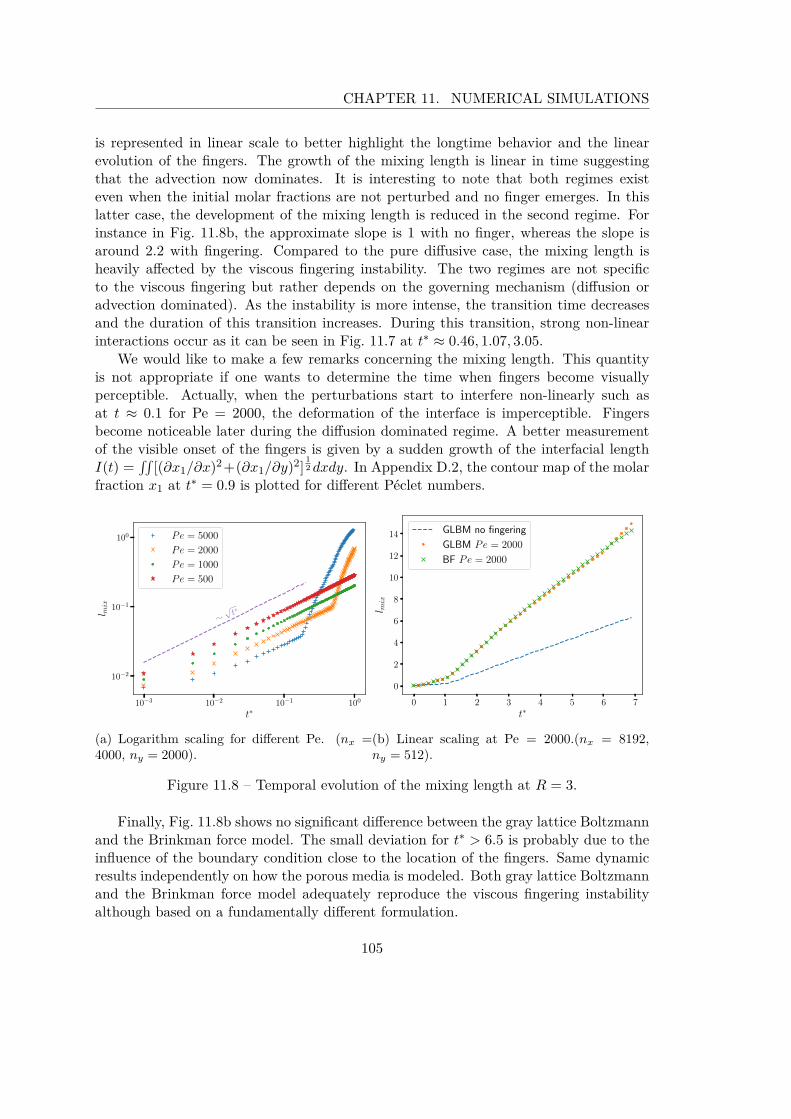
CHAPTER 11. NUMERICAL SIMULATIONS
is represented in linear scale to better highlight the longtime behavior and the linearevolution of the fingers. The growth of the mixing length is linear in time suggestingthat the advection now dominates. It is interesting to note that both regimes existeven when the initial molar fractions are not perturbed and no finger emerges. In thislatter case, the development of the mixing length is reduced in the second regime. Forinstance in Fig. 11.8b, the approximate slope is 1 with no finger, whereas the slope isaround 2.2 with fingering. Compared to the pure diffusive case, the mixing length isheavily affected by the viscous fingering instability. The two regimes are not specificto the viscous fingering but rather depends on the governing mechanism (diffusion oradvection dominated). As the instability is more intense, the transition time decreasesand the duration of this transition increases. During this transition, strong non-linearinteractions occur as it can be seen in Fig. 11.7 at t∗ ≈ 0.46, 1.07, 3.05.
We would like to make a few remarks concerning the mixing length. This quantityis not appropriate if one wants to determine the time when fingers become visuallyperceptible. Actually, when the perturbations start to interfere non-linearly such asat t ≈ 0.1 for Pe = 2000, the deformation of the interface is imperceptible. Fingersbecome noticeable later during the diffusion dominated regime. A better measurementof the visible onset of the fingers is given by a sudden growth of the interfacial lengthI(t) =
∫∫[(∂x1/∂x)2+(∂x1/∂y)2]
12dxdy. In Appendix D.2, the contour map of the molar
fraction x1 at t∗ = 0.9 is plotted for different Péclet numbers.
10−3 10−2 10−1 100
t∗
10−2
10−1
100
l mix
∼√ t∗
Pe = 5000
Pe = 2000
Pe = 1000
Pe = 500
(a) Logarithm scaling for different Pe. (nx =4000, ny = 2000).
0 1 2 3 4 5 6 7
t∗
0
2
4
6
8
10
12
14
l mix
GLBM no fingering
GLBM Pe = 2000
BF Pe = 2000
(b) Linear scaling at Pe = 2000.(nx = 8192,ny = 512).
Figure 11.8 – Temporal evolution of the mixing length at R = 3.
Finally, Fig. 11.8b shows no significant difference between the gray lattice Boltzmannand the Brinkman force model. The small deviation for t∗ > 6.5 is probably due to theinfluence of the boundary condition close to the location of the fingers. Same dynamicresults independently on how the porous media is modeled. Both gray lattice Boltzmannand the Brinkman force model adequately reproduce the viscous fingering instabilityalthough based on a fundamentally different formulation.
105

CHAPTER 11. NUMERICAL SIMULATIONS
11.3 Viscous fingering caused by reverse diffusion
In the previous results, the relation between the viscosity and the concentration isgiven by Eq. (6.40) and not the exponential dependence usually found in the literature(see e.g. [69, 73, 74]). However, the calculated growth rates are in good agreementwith Ref. [74] as shown in Fig. 11.5. This could be expected as for binary mixture Fickor Maxwell approach are equivalent and for species having the same molecular mass,the mixture viscosity µ1 + µ2 has a similar shape as µ0,2e
−Rx1 . For a binary mixturewith species having different molecular masses, the variation of the mixture viscosityaccording to the mixture composition is more complex and can be non-monotonic: themaximum of the mixture viscosity can take place at intermediate molar fractions. Thebehavior of the instability is much more complex. A linear stability analysis shows thatall non-monotonic viscosity profiles, irrespective of their end-point viscosities, becomeunstable [98]. This means that viscous fingering effectively occurs provided only thatthe Péclet number is sufficiently high. Significant differences in the (non-linear) develop-ment of fingers between monotonic and non-monotonic viscosity profiles are explained inRef. [99]. Due to the stable barrier in the non-monotonic profile, fingers spread further indisplacing fluid than in the displaced fluid. More complicated configurations can happenin the case of reacting mixture A + B → C depending the properties of the reactantsand the product. The viscosity profile can be monotonic or non-monotonic and changesin time according to the diffusion and reaction rates. Some phenomena are identical tothose observed in the viscous fingering of a finite slice [100] because of the finite-size ofthe chemical reaction zone. De Wit and other authors study numerically and experi-mentally the influence of the reaction on the viscous fingering instability, see Refs. [101,102, 103, 104], to name a few. Nonetheless, they do not focus on the diffusion involvingby the reactants and the product of the chemical reaction. Most of the analyses assumedgeneralized Fick formulation with the same or a constant Fick diffusion coefficient forall species, which is incorrect as already mentioned in Sec. 3.2 (see e.g. Eq. 3.15).
As we saw the viscous fingering instability is governed by diffusion and viscosity.Contrary to binary mixtures where each species diffuses at an equal rate (D12 = D21), internary mixtures the components can diffuse at different rates (D12 = D13 = D22). Also,multi-component effects such as reverse diffusion, osmotic diffusion and diffusion barriermay take place and the overall diffusion dynamics become more complex. While inbinary mixtures, we have x1 = 1 −x2 and ∇x1 = −∇x2, these constraints on the molarfractions in ternary mixtures are less strict: x1 +x2 +x3 = 1 and ∇x1 +∇x2 +∇x3 = 0.In consequence, since the viscosity depends on the mixture composition, the viscosityevolution could change significantly compared to the binary case. The passage from amixture composed of two species to a mixture composed of three species modify thedynamics of the core ingredients of the viscous fingering instability. In this section, wewill focus on a particular flow configuration in order to highlight the non-negligible effectof ternary mixtures. The case where viscous fingering instability is induced by reversediffusion as, to our knowledge, has not been investigated yet and is presented.
We consider three species having equal molecular masses in different quantities. The
106

CHAPTER 11. NUMERICAL SIMULATIONS
composition of the invading and displaced mixtures is given in Table 11.1. The molarfractions of the first and second components follow a similar step-like pattern as in thecase of the binary mixture. Note that here the first species is less present than thesecond species in the invading mixture and vice versa in the displaced mixture. Thethird species is in equal amounts in both invading and displaced fluids. Before definingadditional physical parameters, we would like to present how this ternary mixture willbe visualized. Each species is associated with a Red-Green-Blue (RGB) color channel.With this strategy, one is able to get the mixture composition from one single color-mapsimilarly to the case of a binary mixture.
Molar fractions Invading fluid Displaced fluidx1 (R) 0.1 0.45x2 (G) 0.45 0.1x3 (B) 0.45 0.45
RGB color
Table 11.1 – Composition of the invading and displaced mixtures.
We set the diffusion coefficients such as the third species will be subject to reversediffusion. This can be estimated by means of the generalized Fick formulation in thecase of pure diffusion (Sec. 3.2):
J2 = −ctD22∇x2 − ctD23∇x3, (11.14)J3 = −ctD32∇x2 − ctD33∇x3, (11.15)
and J1 = −J2 − J3. (11.16)
We want J3 < 0 and since ∇x3 = 0 and ∇x2 = (< 0, 0)T , we should have D32 < 0. Werecall the definition of the Fick diffusion coefficients from Eqs. (3.15) and (3.16):
D33 = D13 (x3D12 + (1 − x3)D23) /D, (11.17)D32 = x3D12 (D13 − D23) /D, (11.18)
with D = x1D23 + x2D13 + x3D23. (11.19)
Hence, we should set D23 > D13. We choose the following diffusion matrix
Dmn = LrefU
Pe
⎛⎜⎝ 0 1 0.11 0 1
0.1 1 0
⎞⎟⎠ , (11.20)
with Pe = 5000, U = 2 × 10⁻³lu, the Darcy number is unchanged Da = 6.25 × 10⁻⁸
and the porous medium is simulated using the Brinkman force strategy. Pure viscositiesare set based on Re0,1 = 10 and R12 = ln(µ0,1/µ0,2) = 0, R13 = ln(µ0,1/µ0,3) = 3. Thefirst and second components which vary on either side of the miscible interface havethe same pure viscosity whereas the pure viscosity of the third species present in equal
107

CHAPTER 11. NUMERICAL SIMULATIONS
Figure 11.9 – Snapshot of the viscous fingering induced by reverse diffusion at t∗ = 1.8.The whole domain (nx = 4000, ny = 2000) is plotted using the same aspect ratio forboth x and y-axes. Each species is associated with a RGB channel. An enlargement isprovided and contour-plots for x1 = x2 = 0.275 and x3 = 0.45 are drawn.
amount in the domain is approximately twenty times lower. Compare to the binary case,the boundary conditions are modified. We still use the non-equilibrium bounce-back,which prescribes for each species either a pressure or a velocity at boundary nodes. Fora mixture composed of two species, we impose a velocity and small changes of partialpressure, mixture composition, occur. In the case of three components, the variationof the mixture composition at boundaries compared to the initial target fluid becomesimportant so we choose to impose the pressure at both boundaries using Eq. (11.4)adapted for three species. However, this introduces a decrease of the inlet velocity astime progresses which means that the Péclet number loses some of its meaning.
Both invading and displaced mixtures have the same viscosity. If the diffusion coef-ficients have all the same value, no fingers appear. In this specific case, this reduces toa binary mixture as the first and second species are identical and, as expected, the flowis stable when both invading and displaced fluid viscosities are equal. However if weset D13 = 0.1D12 = 0.1D23, fingers develop as pictured in Fig. 11.9 although the initialconfiguration is stable. Small fingers develop at latter times compared with the binarycase and their blue color suggests that they are mainly composed of the third species.From the enlargement, one can also notice that the interface of the first (red) species isalso perturbed.
The fingering is actually caused by the reverse diffusion as inferred by Fig. 11.10.At the beginning of the simulation, the third and less viscous component is uniformlypresent. However, the third (blue) species starts to diffuse from the displaced to theinvading mixtures (osmotic diffusion) and keeps diffusing against its concentration gra-dient (reverse diffusion) and the main flow. In consequence, at t∗ = 0.1 a local increaseof the concentration of the third species is clearly visible and is followed by a local de-crease. This change of the mixture composition affects significantly the properties of the
108

CHAPTER 11. NUMERICAL SIMULATIONS
140 160 180 200 220 240 260
x
0.10
0.15
0.20
0.25
0.30
0.35
0.40
0.45
Mol
arfr
acti
ons
t∗ = 0.0
0.02
0.04
0.06
0.08
0.10
0.12
0.14
0.16
0.18
Vis
cosi
ty
300 350 400 450 500
x
0.10
0.15
0.20
0.25
0.30
0.35
0.40
0.45
0.50
Mol
arfr
acti
ons
t∗ = 0.1
0.025
0.050
0.075
0.100
0.125
0.150
0.175
0.200
Vis
cosi
ty
2800 3000 3200 3400 3600
x
0.10
0.15
0.20
0.25
0.30
0.35
0.40
0.45
Mol
arfr
acti
ons
t∗ = 1.8
0.02
0.04
0.06
0.08
0.10
0.12
0.14
0.16
0.18
Vis
cosi
ty
Figure 11.10 – Evolution at different times of the mean molar fraction over the transversedirection, continuous lines, and the mean partial viscosity over the transverse direction,dashed lines. Viscosities are normalized by the pure viscosity µ0,1. Red, first species;green, second species; blue, third species. Orange stand for the mean mixture viscosityover the transverse direction.
mixture and results locally in a decrease followed by an increase of the mixture viscositythat will trigger the instability. The effective viscosity ratio is lower and makes the in-stability less intense compared to the binary case. We recall that the mixture viscosityis computed a posteriori whereas only partial viscosities are employed in the model. Att∗ = 1.8 the mean transverse molar fraction of the third species fluctuates because ofthe presence of fingers as show in Fig. 11.9.
From the enlargement of Fig. 11.9, one can observe the variation of the interfacebetween the invading and the displaced mixtures. If the blue-colored fingers highlightsthe displacement of the third species because of the instability, the contour-plots showalso some variations of the interface for the first (red) species. In figure 11.11, the molarfraction of each species is plotted. The right figure shows that some fingers are composedof a very high concentration of the third species. Counter-fingers, which moves from theright to the left, have a minimal molar fractions of x3 = 0.33. We underline that reversediffusion should still occur and tends to reinforce the fingers of medium concentration andlimits the development of counter-propagating fingers of low concentration. However,the third species is not the only one to be subject to fingering. The interface of thefirst species is also significantly deformed. The invading fluid penetrates primarily thedisplaced fluid through the low viscosity fingers caused by the third species and avoidsthe zone of high viscosity. In consequence, small fingers of low concentration of thefirst species develop. One can notice that in contrary almost no fingering for the secondspecies appears. The interface seems symmetrically diffuse. This phenomenon can beexplained by means of the diffusion matrix Eq. (11.20). Since D13 < D12, the first speciesdiffuses predominantly in the second species compared to the third species that is whysmall fingers of low concentration of the first species are visible in fingering caused bythe third species. Concerning the second component, we have D12 = D23 and the secondspecies diffuses in both species equitably.
We emphasize the importance of the ternary diffusion on the instability onset. Diffu-sion governs the reverse fingering, its strength, and its life span until the diffusion barrier
109

CHAPTER 11. NUMERICAL SIMULATIONS
2600 3100 3600
600
800
1000
1200
1400
x1
2600 3100 3600
x2
2600 3100 3600
x3
0.100 0.275 0.450
Mole fraction0.29 0.33 0.45 0.61
Mole fraction
Figure 11.11 – Color-map of the molar fraction at t∗ = 1.8 for each species. Portion ofthe domain (nx = 4000, ny = 2000).
point. Diffusion also controls the growth of the perturbations and stabilizes the flow asin the binary case. In the present configuration, we deliberately showcase the significantinfluence of reverse diffusion on a flow, which is initially stable. With the numbers ofpossible different configurations of viscosities and diffusion coefficients, a complete para-metric study is out of the scope of the present work. Nonetheless, we expect to see moresubtle or on the contrary dramatic changes due to the multi-component effects comparedto the viscous fingering of two species.
110

Chapter 12
Synthesis
This last part is dedicated to the simulation of the viscous fingering instability. Theinteraction between the two (or three) miscible components are described by the afore-mentioned miscible lattice Boltzmann model. The core ingredients of the instability arerelated to the molecular diffusion and the viscosity, or more specifically inter-molecularfriction forces and partial viscosities in our model. Generally, the instability occurswhen a less viscous fluid displaces a more viscous fluid in a porous medium. Thus weinvestigate two strategies to mimic the effect of the porous medium: the gray latticeBoltzmann and Brinkman force models.
The viscous fingering is first studied in the case of a binary mixture. At early timesin the linear regime, the growth rate of the perturbation is computed for different Pécletnumbers. The growth rate, as well as the most dangerous and the cutoff numbers,increase with the Péclet number. A good agreement is found with a linear stabilityanalysis where a quasi-steady-state-approximation is used. For intermediate times wherestrong linear interactions take place, the development of the instability is describedglobally through the mixing length. A high Péclet number leads to a more intenseinstability. Two regimes are visible. The growth of the mixing length is first dominatedby diffusion and then by convection.
For both early and intermediate times investigated here, the gray lattice Boltzmannand Brinkman force models lead to equivalent results. The comparison with the lit-erature, quantitatively for early times and qualitatively for intermediate times agreeswell. This is very encouraging and gives much credence to the proposed lattice Boltz-mann model. Indeed with a different approach, we recover accurately the physics of theviscous fingering.
Finally, the behavior of the instability can dramatically change for a mixture of threeand more species compared to the binary case. For instance, viscous fingering could beinduced by reverse diffusion despite having a stable initial flow configuration.
111


Conclusion
113


Conclusion
The first part of this thesis covers the basics of the lattice Boltzmann method. Start-ing from the kinetic theory of gas and the Boltzmann equation, a discrete formulation isproposed. A major tool to obtain the resulting macroscopic equations is the Chapmanand Enskog expansion procedure. The relaxation time is thus related to the viscous dis-sipation. Independently, we introduce the Maxwell-Stefan approach to deal with purediffusion between species. This approach is more convenient and has a more rigorousphysical meaning for three and more species compared to the traditional Fick formu-lation. Besides, we showcase some non-trivial diffusion effects that may occur duringthe diffusion of three and more components such as osmotic diffusion, reverse diffusion,and diffusion barrier. The fundamental contribution of this thesis is to combine theseideas and propose a lattice Boltzmann model for miscible gases in the second part ofthis thesis.
Different lattice Boltzmann models for multi-component flows already exist. Sincethere is no unique and generally accepted BGK-like collision operator, each model de-pends on the underlying kinetic theory chosen. However, for all models in the case ofbinary mixtures, the variation of momentum induced by the collision has a similar formas the inter-molecular friction force, i.e., a coefficient multiplied by the velocity differ-ence of the two species. Any previous model requires to heavily modified the collisionstep compared to the standard formulation so as to take into account the interactionsbetween components. This increase of complexity makes the algorithm more compu-tationally expensive, and above all, it cannot be easily incorporated in existing LBMcodes. The collision being the cornerstone of the LBM, changing the collision meansusually rewrite the code entirely. In the proposed approach, the standard equilibrium isemployed combined with the inter-molecular friction force. Much less effort is thereforeneeded to upgrade a single-fluid code to take into account diffusion between multiplespecies. The viscous dissipation is related to the relaxation toward the equilibriumstate, and the molecular diffusion is associated with the inter-molecular diffusion force.To calculate the transport coefficients, we make use of the kinetic theory of gases. Inaddition to the (Maxwell-Stefan) diffusion coefficient, a partial viscosity is also definedfor each species. The problem of a fixed lattice speed of sound peculiar to the LBM iscircumvented by using an artificial force to modify the species equation of state accordingto the molecular mass of the component. Excellent agreements are found against ana-lytical, experimental, and numerical results. The complex diffusion dynamics of threeand more species is recovered, and the proposed model is capable of simulating osmoticdiffusion, reverse diffusion, and diffusion barrier phenomena. After being validated thebasic features of our model, we apply it to the viscous fingering instability and discussthe results obtained in the last part of the thesis.
The simulation of the viscous fingering instability is achieved by considering twospecies in different proportions in a porous medium: a less viscous mixture displacing amore viscous mixture. The core ingredients of the instability are the diffusion and theviscosity contrast between the components. Two strategies are investigated to mimic theeffects of the porous medium. The gray lattice Boltzmann and Brinkman force models,although based on fundamentally different approaches, give in our case equivalent results.
115

Conclusion
For early times, we focus on the growth rate of the perturbation and the influence of thePéclet number. Comparisons with linear stability analyses agree well with the growthrate calculated from the simulations. For intermediate times, the evolution of the mixinglength can be divided into two stages dominated first by diffusion then by convection,as found in the literature. The whole physics of the viscous fingering is thus accuratelysimulated. Nevertheless, multi-component diffusion effects are usually not taken intoaccount in the case of viscous fingering with three and more species. These effectsare non-negligible as we showcase an initial stable configuration that becomes unstable.The reverse diffusion induces fingering whose impact depends on the diffusion betweenspecies. After a successful application of the proposed model on the viscous fingering,we are longing to tackle other problems involving multi-species flows.
PerspectivesThe derivation of the proposed model is rigorously correct only for dilute gases. We
could, to a certain extent, apply it to liquids and general gases. The Maxwell-Stefanequations are also valid for low and high densities, liquids, and polymers, so we canassume that the inter-molecular friction force still adequately describe the moleculardiffusion in these cases. The partial pressure is not well defined for a non-ideal gas,and its gradient should be substituted by the gradient of chemical potential. Transportcoefficients should be calculated using the Eyring (liquids) or Enskog (dense gases) ki-netic theories [1]. More fundamental studies are required on the model. For instance,the simulation of a mixing layer between three species could point out some interestingmechanisms. A comparison with a recent and well-documented experiment would bebeneficial. A starting point could be to quantify the influence of the partial viscositiesbased on the experiments of variable viscosity jet flows carried out in Ref. [105].
Concerning the viscous fingering simulations, different configurations with the ternarymixture should be considered. A parametric study could be performed and draw outthe first results obtained here. Another possibility is to model the pores at a global levelinstead of mimicking the porous medium. In spite of being computationally expensive,this simulation would highlight the different scale of the porous medium in play. Fi-nally, we could notice that the porous drag force has a similar form as the Boussinesq’sapproximation made in double-diffusive convection problems in oceans, and opens newperspectives for the proposed model.
The following publications are related to this work (see also Appendix E):— Lucien Vienne, et al. “Lattice Boltzmann method for miscible gases: A forcing-
term approach”. In: Physical Review E. [106]— Lucien Vienne, et al. “Viscous fingering simulation by the lattice Boltzmann
method”. Under preparation.
116

Appendix
117

A Hermite polynomials and Gauss-Hermite quadrature 121A.1 Hermite polynomials 1-dimensional space . . . . . . . . . . . . . . . . . . 121A.2 Hermite polynomials in d-dimensional space . . . . . . . . . . . . . . . . . 122A.3 Gauss-Hermite quadrature . . . . . . . . . . . . . . . . . . . . . . . . . . . 123
B Programming considerations 127B.1 Code . . . . . . . . . . . . . . . . . . . . . . . . . . . . . . . . . . . . . . . 127B.2 HPC . . . . . . . . . . . . . . . . . . . . . . . . . . . . . . . . . . . . . . . 128
C Kinetic theory for the calculation of transport coefficients 129C.1 Omega-integrals . . . . . . . . . . . . . . . . . . . . . . . . . . . . . . . . 129C.2 Wilke’s law . . . . . . . . . . . . . . . . . . . . . . . . . . . . . . . . . . . 130C.3 A more common formulation of the diffusion coefficient . . . . . . . . . . 132
D Viscous fingering 135D.1 Most dangerous and cutoff wave numbers . . . . . . . . . . . . . . . . . . 135D.2 Color maps of the molar fraction for different Péclet numbers . . . . . . . 135
E Parallel activities 137E.1 Conferences and discussions . . . . . . . . . . . . . . . . . . . . . . . . . . 137E.2 Ercoftac Montestigliano spring-school . . . . . . . . . . . . . . . . . . . . 137
F Résumé étendu des travaux de la thèse en français 143
119


Appendix A
Hermite polynomials andGauss-Hermite quadrature
A.1 Hermite polynomials 1-dimensional spaceHermite polynomials are an orthogonal polynomials sequence defined by the weight
functionω(x) = 1√
2πe−x2/2, (A.1)
which is normalised so that∫∞
−∞ ω(x)dx = 1. The expression of the weight function mayslightly vary in the literature and accordingly the definition of the Hermite polynomialscould be a little different. The n-th order of Hermite polynomials are constructed fromthe Rodrigues’ formula
H(n)(x) = (−1)n 1ω(x)
dn
dxnω(x), (A.2)
and the first few polynomials are
H(0)(x) = 1, (A.3)H(1)(x) = x, (A.4)H(2)(x) = x2 − 1, (A.5)H(3)(x) = x3 − 3x. (A.6)
One can find the recursion formula
H(n+1)(x) = xH(n)(x) − d
dxH(n)(x) = xH(n)(x) − nH(n−1)(x) (A.7)
One of the interesting properties of the Hermite polynomials is their orthogonality withrespect to the weight function ω(x)∫ ∞
−∞ω(x)H(m)(x)H(n)(x)dx = n!δmn, (A.8)
121

APPENDIX A. HERMITE POLYNOMIALS AND GAUSS-HERMITEQUADRATURE
where δmn is the Kronecker symbol, i.e., δmn = 1 if m = n and 0 otherwise.Any function f that is square integrable can be expanded in terms of Hermite poly-
nomials asf(x) =
∞∑n=0
a(n)H(n)(x). (A.9)
The Hermite expansion coefficient a(n) can computed by multiplying the previous equa-tion Eq. (A.9) by ω(x)Hm(x) and integrating∫ ∞
−∞ω(x)Hm(x)f(x)dx =
∞∑n=0
a(n)∫ ∞
−∞ω(x)Hm(x)H(n)(x)dx = m! a(m) (A.10)
a(m) =∫ ∞
−∞
1m!ω(x)Hm(x)f(x)dx (A.11)
where the orthogonal property of the Hermite polynomials has been used to simplify thesummation. Instead of using Eqs. (A.9) and (A.11), the following alternative expressionis preferred
f(x) = ω(x)∞∑
n=0
1n!a
(n)H(n)(x), (A.12)
where the expansion coefficient a(n) is given by
a(n) =∫ ∞
−∞Hm(x)f(x)dx. (A.13)
This (Gram-Charlier) series converges only if f approach zero faster than e−x2/4. Inpractice, this assumption is correct for gases that are not too far from the equilibriumstate (at the equilibrium: f ∼ e−x2/2) [12].
A.2 Hermite polynomials in d-dimensional spaceAll of these previous expressions can be generalized to a d-dimensional space as shown
by Grad [107].
H(n)i (x) = (−1)n 1
ω(x)∇ni ω(x), ω(x) = 1
(2π)d/2 e−x2/2 (A.14)
where x2 = x · x and the operator ∇ni is equivalent to
∇ni = ∇n
(i1,··· ,in) = ∂
∂xi1· · · ∂
∂xin
. (A.15)
With this definition, the first few polynomials are
H(0)(x) = 1, (A.16)
H(1)i (x) = xi, (A.17)
H(2)ij (x) = xixj − δij , (A.18)
H(3)ijk(x) = xixjxk − xiδjk − xjδki − xkδij . (A.19)
122

APPENDIX A. HERMITE POLYNOMIALS AND GAUSS-HERMITEQUADRATURE
The orthogonal relation becomes∫ω(x)H(m)
i (x)H(n)j (x)dx =
d∏p=1
np! δmnδnij , (A.20)
where δnij is the generalization of the Kronecker symbol, which is equal to 1 if (i1, · · · , in)
is a permutation of (j1, · · · , jn) and 0 otherwise. For i = (i1, i2, i3, i1), n1 = 2, n2 = 1,and n3 = 1.
Finally, a function f that is square integral can be expanded as
f(x) = ω(x)∞∑
n=0
1n!a
(n)i H
(n)i (x), with (A.21)
a(n)i =
∫f(x)H(n)
i (x)dx (A.22)
We point out that both a(n)i and H
(n)i are tensors of rank n and this leads to this
equivalent formulation
f(x) = ω(x)
⎛⎝a(0)H(0) +d∑
i=1a
(1)i H
(1)i +
d∑i,j=1
a(2)ij H
(2)ij +
d∑i,j,k=1
a(3)ijkH
(3)ijk + · · ·
⎞⎠ (A.23)
A.3 Gauss-Hermite quadratureA Gaussian quadrature approximates the following integral with only q points,∫ b
aω(x)f(x)dx =
q∑α=0
ωαf(xα), (A.24)
where ω(x) is an arbitrary weight function, ωα are the weight of the quadrature, and xα
are the abscissas of the quadrature, which are the roots of the orthogonal polynomialsfor the scalar product
∫ ba ω(x)g(x)h(x)dx. This quadrature is exact for any polynomials
f of degree 2q − 1 or less.In particular if we choose the weight function as Eq. (A.1), the Gauss-Hermite
quadrature is obtained. We recall that the expression of the weight function may slightlyvary in the literature, and so as the weights and the abscissas. The abscissas are thenthe roots of the Hermite polynomials and the corresponding weights are [5]
ωα = q![qH(q−1)(xα)
]2 . (A.25)
Using Eqs. (A.3-A.6), the Gauss-Hermite quadrature up to q = 3 is constructed as shownin Table A.1.
The Gauss-Hermite quadrature can be generalized into a d-dimensional space.∫ω(x)f(x)dx =
qd∑α=0
ωαf(xα) (A.26)
123

APPENDIX A. HERMITE POLYNOMIALS AND GAUSS-HERMITEQUADRATURE
Number of abscissas Polynomial degree Abscissas Weightq 2q − 1 xα ωα
1 1 0 12 3 −1, 1 1/2, 1/23 5 −
√3, 0,
√3 1/6, 2/3, 1/6
Table A.1 – Gauss-Hermite quadrature up to q = 3, which is exact for polynomials ofdegree 5 or less.
For instance, if we want to approximate a fifth-degree polynomial, the one-dimensionalquadrature for q = 3 is used repeatedly. For a two-dimensional space, we find a ninepoints quadrature presented in Table A.2.
α 1 2 − 5 6 − 9
Abscissas (0, 0) (±√
3, 0) (±√
3,±√
3)(0,±√
3)Weight 4/9 1/9 1/36
Table A.2 – Gauss-Hermite quadrature for a fifth-degree polynomial in two-dimensionalspace.
Similarly for a 3-dimensional space, the quadrature is obtained by a production of the1-dimensional formula (see Table A.3). From the 27 points quadrature, one can derive
α 1 2 − 7 8 − 19 20 − 27
Abscissas (0, 0, 0)(±
√3, 0, 0) (±
√3,±
√3, 0)
(±√
3,±√
3,±√
3)(0,±√
3, 0) (±√
3, 0,±√
3)(0, 0,±
√3) (0,±
√3,±
√3)
Weight 8/27 2/27 1/54 1/216
Table A.3 – Gauss-Hermite quadrature for a fifth-degree polynomial in three-dimensionalspace.
equivalent quadratures with less points, 15 (Table A.4) and 19 (Table A.4) abscissas [5].Other and high order quadratures are possible [5] but only a few, like those presented
here, coincide with normal Cartesian coordinates. The use of a quadrature compatiblewith a uniform Cartesian grid results in a perfect streaming step.
124

APPENDIX A. HERMITE POLYNOMIALS AND GAUSS-HERMITEQUADRATURE
α 1 2 − 7 8 − 15
Abscissas (0, 0, 0)(±
√3, 0, 0)
(±√
3,±√
3,±√
3)(0,±√
3, 0)(0, 0,±
√3)
Weight 2/9 1/9 1/72
Table A.4 – Alternative Gauss-Hermite quadrature with 15 abscissas for a fifth-degreepolynomial in three-dimensional space.
α 1 2 − 7 8 − 19
Abscissas (0, 0, 0)(±
√3, 0, 0) (±
√3,±
√3, 0)
(0,±√
3, 0) (±√
3, 0,±√
3)(0, 0,±
√3) (0,±
√3,±
√3)
Weight 1/3 1/18 1/36
Table A.5 – Alternative Gauss-Hermite quadrature with 19 abscissas for a fifth-degreepolynomial in three-dimensional space.
125


Appendix B
Programming considerations
B.1 Code
The code employs in the present work is written from scratch using a combination ofFORTRAN and Python. All the computations are done in FORTRAN routines whichare wrapped in Python through the F2PY wrapper. Python is only used for the pre-processing, the scheduler and the data tree. Therefore, we join the advantages of bothlanguages: the fast execution of FORTRAN and the ease of use and the plethora oflibraries of Python.
The lattice Boltzmann algorithm involves only a few numerical operations and ismainly limited by the memory access speed. Most of the time spent in LBM is due tothe memory transfer and not computations. Different possibilities exist to store datafrom slow to high-speed access: disk, memory, caches, and registers. Usually the pro-gram stores variables in the main memory and when computations are required, data aretransferred from the memory to the registers. If the same data are reused again, a copymay be made and store in the caches to speed-up further accesses. Most optimizationsof memory-bound programs are performed by reusing as much as possible the caches.Indeed when a data is copied to the caches, nearby data are also copied too. Memorylayout has thus a significant impact on the performance. The lattice Boltzmann methodis primarily composed of two steps: collision and streaming. Unfortunately, the optimalmemory layout is different for both of these steps. In collision, the distribution functionsfrom all the directions α at a single node x are needed (f [α,x] is optimal in FORTRANcolumn-major order) whereas the streaming steps requires all the neighboring node foreach direction (f [x, α] is optimal in FORTRAN column-major order). A wrong mem-ory layout could be catastrophic and results in an algorithm at least two times slower.No general rule exists and the most efficient memory layout depends strongly on thecomputing architecture (caches sizes and other optimizations), and the domain size sim-ulated and the number of velocities (9 in 2D, 15, 19, or 27 in 3D). We recommend totest and adapt the memory layout specifically to the target machine.
We would like also to provide two recommendations. First, when using a MRTcollision operator, one should carry out the matrix-vector multiplication by hand and
127
APPENDIX B. PROGRAMMING CONSIDERATIONS
code the result. Second, when performing the streaming step, do not use two arraysfor the post-collision and post-steaming distribution functions. Only one array for thedistribution functions is needed. During the streaming, the array has simply to bebrowsed in the standard way or in the reverse order depending on the memory layoutand velocities to update and avoid to overwrite the relevant distribution functions.
B.2 HPCHigh-Performance Computing denotes strategies to improve and achieve a high level
of performance. As we mentioned before the limiting factor in the Lattice Boltzmannmethod is data transfers. One possible way to improve the code is to use multiplecomputational units, from hundreds to thousands, for the same problem and therebydata transfers are carried out in parallel. In the current code (D2Q9 and D3D19), thisis accomplished by the means of the Message Passing Interface (MPI) paradigm. Theproblem domain is divided into multiple sub-domains where calculations are performedindependently and synchronization is realized by sending-receiving messages. In practice,the computational domain is expanded with a layer of ghost nodes, which store a copyof the neighboring node from the adjacent MPI process and are updated just beforethe non-local streaming step. Reading and writing data in a unique file is also donein parallel using MPI dedicated functions and data-types. Other strategies have beeninvestigated and tested to improve the code performance such as vectorizations, openMP,openACC (GPU), and cache blocking. Nonetheless, code optimization although beingimportant is very time-consuming and we decide to stay with a standard MPI domaindecomposition. We insist again that the memory layout impact is significant and maychange compared to the standard sequential case, especially for GPU architectures.
The author acknowledges the "Institut du Développement et des Ressources en In-formatique Scientifique" (IDRIS) for their advanced training courses regarding MPI,vectorization, openMP, and openACC.
128

Appendix C
Kinetic theory for the calculationof transport coefficients
C.1 Omega-integralsWe specify the expression of the Ω-integrals. We recall that the interactions of a
similar pair of molecules can be approximated by the Lennard-Jones potential.
φ(r) = 4ϵ[(
σ
r
)12−(σ
r
)6], (C.1)
where r is the distance between the molecules, σ the collision diameter, and ϵ the depthof the potential well. For a dissimilar (m,n) pair of molecules , we use the followingstandard mixing rules:
σmn = (σm + σn)/2, (C.2)ϵmn =
√ϵmϵn, (C.3)
1ψmn
= 1Mm
+ 1Mn
. (C.4)
Unlike the rigid sphere model, the Lennard-Jones potential is a physically realisticpotential, and the Ω-integrals can not be calculated analytically. However, we computethe Ω-integrals for the rigid sphere and introduce the Ω⋆ ratio, which embodies thedeviation of the Ω-integrals between the Lennard-Jones and rigid sphere potentials.
Ω⋆(i,j)mn = Ω(i,j)
mn /Ωrs(i,j)mn (C.5)
with
Ωrs(i,j)mn =
√kBT
2πψmn
(j + 1)!2
[1 − 1
21 + (−1)i
1 + i
]π(σmn)2. (C.6)
Ω⋆(i,j)mn depends only on T ⋆ = TkB/ϵmn and its value is obtained from a fitted curve
computed from a numerical integration [59, 108]. For more details about the potentials,we invite the reader to read the Chapter 8 of Ref. [1].
129
APPENDIX C. KINETIC THEORY FOR THE CALCULATION OF TRANSPORTCOEFFICIENTS
Despite the derivation is rigorously correct only for dilute gases, we could to a certainextent, apply these results to liquids and dense gases by means of the Eyring and Enskogtheories, respectively.
C.2 Wilke’s lawThe partial viscosities are obtained by solving the linear system Eq. (6.37). This
approach is computationally expensive since this system has to be solved for each timestep on each grid point. In this section, we propose to derive a simpler expression forpartial viscosities. We will combine some assumptions made in Ref. [1] ( §8.2.iii) andadditional approximations suggested in Ref. [66]. Equations (6.38) and (6.39) can bewritten as
Pmm = 1µ0,m
+N∑
n=m
1kBT
xn
xm
323
MmMn
(Mm + Mn)2 Ω(1,1)mn ×
(1 + 3
5Mn
MmA∗
mn
)(C.7)
and for n = m,
Pmn = −323
1kBT
MmMn
(Mm + Mn)2 Ω(1,1)mn
(1 − 3
5A∗mn
)(C.8)
where A∗mn = Ω∗(2,2)/Ω∗(1,1) and µ0,m is the pure viscosity of species m
µ0,m = 5kBT/(8Ω(2,2)mm ). (C.9)
In general, the off-diagonal terms are small in comparison with the diagonal elements. IfA∗
m,n = 5/3 ∀(m,n), the off-diagonal terms vanish exactly. This assumption is proposedin Ref. [1] ( §8.2.iii). When this assumption is made, the diagonal elements become
Pmm = 1µ0,m
+N∑
n=m
1kBT
xn
xm
323
Mn
(Mm + Mn)Ω(1,1)mn . (C.10)
and for n = m,Pmn = 0 (C.11)
Using Eq. (6.43), we rewrite Eq. (C.10) as
Pmm = 1µ0,m
+N∑
n =m
xn
xm
2kBT
pMmDmn. (C.12)
This yield to our first approximation of the partial viscosity according to the diffusioncoefficients
µm =
⎡⎣ 1µ0,m
+ 2RTpxmMm
N∑n =m
xn
Dmn
⎤⎦−1
, (C.13)
130
APPENDIX C. KINETIC THEORY FOR THE CALCULATION OF TRANSPORTCOEFFICIENTS
by definition, we have Mm = MmNa where Na is the Avogadro number and Mm isthe molar mass of species m and the universal gas constant R = kBNa. The numericalconstant 2 is often replaced by the empirical value 1.385 [109].
In the next paragraph, we make further assumptions result in an approximation ofthe partial viscosity in terms of pure viscosities. From Eq. (C.5) and Eq. (C.6), we write
Ω(1,1)mn = Ω∗(1,1)
mn ×
√kBTπ
2(Mm + Mn)
MmMn
14 [σm + σn]2 . (C.14)
For collisions between particles of the same species, we can invert Eq. (C.6),
σm = σmm =[Ωrs(1,1)
mm ×√
Mm
kBTπ
] 12
(C.15)
but the expression of Ωrs(1,1)mm can be computed from the pure viscosity
Ωrs(1,1)mm = Ω(2,2)
mm
2A∗mmΩ∗(1,1)
mm
= 316kBT
1Ω∗(1,1)
mm µ0,m
. (C.16)
Thus by combining Eqs. (C.15) and (C.16) into Eq. (C.14), we get
Ω(1,1)mn = Ω∗(1,1)
mn × 364
√2kBT
√Mm + Mn
MmMn
×[(
Ω∗(1,1)mm µ0,m
)− 12 (Mm)
14 +
(Ω∗(1,1)
nn µ0,n
)− 12 (Mn)
14
]2.
(C.17)
Let also assume as suggested in Ref. [66]
Ω∗(1,1)mn
Ω∗(1,1)mm
≈ 1 and Ω∗(1,1)mn
Ω∗(1,1)nn
≈ 1. (C.18)
These previous expressions do not necessary need to be viewed as equal. Therefore, theerror caused by both assumptions may fortuitously cancel in Eq. (C.17). If we factorize,Ω(1,1)
mn becomes
Ω(1,1)mn = 3
64√
2kBT
√Mm + Mn
Mn× 1µ0,m
⎡⎣1 +(µ0,m
µ0,n
) 12 (Mn
Mm
) 14
⎤⎦2
. (C.19)
Finally the diagonal elements Pmm Eq. (C.10) can be computed as
Pmm = 1µ0,m
+N∑
n=m
12√
2xn
xm
( Mn
Mm + Mn
) 12
× 1µ0,m
⎡⎣1 +(µ0,m
µ0,n
) 12 (Mn
Mm
) 14
⎤⎦2
.
(C.20)
131

APPENDIX C. KINETIC THEORY FOR THE CALCULATION OF TRANSPORTCOEFFICIENTS
The partial viscosities are then equal to
µm = µ0,m
1 +∑N
n=mxnxm
Φmn
= xmµ0,m∑Nn xnΦmn
(C.21)
with
Φmn = 12√
2
(1 + Mm
Mn
)− 12
⎡⎣1 +(µ0,m
µ0,n
) 12 (Mn
Mm
) 14
⎤⎦2
. (C.22)
This formulation of the partial viscosities is much simpler than solving the linear systemEq. (6.37) since the former only involves the molar fractions, and the pure viscosity andthe molar mass of each species. If one defines the mixture viscosity as
µmixture =N∑m
µm, (C.23)
Wilke’s law for the viscosity of a gas mixture is then recovered [66]. The summationof partial viscosities over all species results in Wilke’s law. Therefore, Wilke’s law isa consequence and not the origin of the derivation of the partial viscosities. Indeedrecovering Wilke’s law is consistent with the mixture momentum equation.
In figure C.1, viscosities of binary mixtures He-Ar and CO2-C3H8 calculated byinversion of the matrix are plotted as well as the approximated solution. Concerningthe system inversion, the Ω-integrals are first computed for the rigid sphere model usingTable. C.1 and the deviation between the Lennard-Jones and rigid sphere potentials Ω∗
is obtained by a fitting curve from a numerical integration [59, 108].
m Ar He CO2 C3H8Mm [g/mol] 39.948 4.0026 44.0095 44.0956ϵm/kB [K] 124. 35.70 190. 206.σm [nm] 0.3418 0.2576 0.3996 0.5240
Table C.1 – Kinetic constants from Ref. [1].
C.3 A more common formulation of the diffusion coeffi-cient
The notation used here is based on Molecular theory of gases and liquids by Hirschfelder,Curtiss, and Bird [1]. A more common formulation for the diffusion coefficient is givenby Hirschfelder-Bird-Spotz or in chapter 11 of Ref. [108] and can be obtained followingthe definitions given in Appendix C.1.
Dmn = Dnm = 3(Mm + Mn)16pMmMn
(kBT )2
Ω(1,1)mn
. (C.24)
132
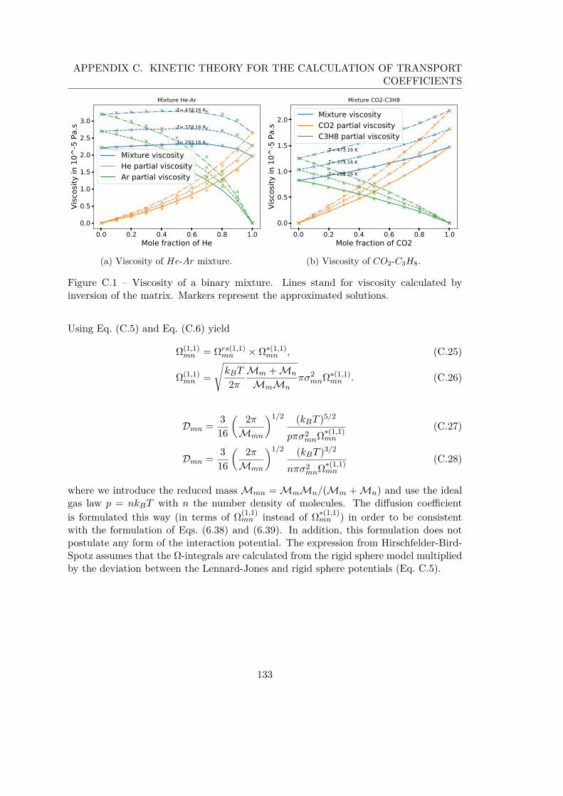
APPENDIX C. KINETIC THEORY FOR THE CALCULATION OF TRANSPORTCOEFFICIENTS
0.0 0.2 0.4 0.6 0.8 1.0Mole fraction of He
0.0
0.5
1.0
1.5
2.0
2.5
3.0
Visc
osity
in 1
0^-5
Pa.
s
T= 293.16 K
T= 373.16 K
T= 473.16 KMixture He-Ar
Mixture viscosityHe partial viscosityAr partial viscosity
(a) Viscosity of He-Ar mixture.
0.0 0.2 0.4 0.6 0.8 1.0Mole fraction of CO2
0.0
0.5
1.0
1.5
2.0
Visc
osity
in 1
0^-5
Pa.
s
T= 293.16 K
T= 373.16 K
T= 473.16 K
Mixture CO2-C3H8
Mixture viscosityCO2 partial viscosityC3H8 partial viscosity
(b) Viscosity of CO2-C3H8.
Figure C.1 – Viscosity of a binary mixture. Lines stand for viscosity calculated byinversion of the matrix. Markers represent the approximated solutions.
Using Eq. (C.5) and Eq. (C.6) yield
Ω(1,1)mn = Ωrs(1,1)
mn × Ω∗(1,1)mn , (C.25)
Ω(1,1)mn =
√kBT
2πMm + Mn
MmMnπσ2
mnΩ∗(1,1)mn . (C.26)
Dmn = 316
( 2πMmn
)1/2 (kBT )5/2
pπσ2mnΩ∗(1,1)
mn
(C.27)
Dmn = 316
( 2πMmn
)1/2 (kBT )3/2
nπσ2mnΩ∗(1,1)
mn
(C.28)
where we introduce the reduced mass Mmn = MmMn/(Mm + Mn) and use the idealgas law p = nkBT with n the number density of molecules. The diffusion coefficientis formulated this way (in terms of Ω(1,1)
mn instead of Ω∗(1,1)mn ) in order to be consistent
with the formulation of Eqs. (6.38) and (6.39). In addition, this formulation does notpostulate any form of the interaction potential. The expression from Hirschfelder-Bird-Spotz assumes that the Ω-integrals are calculated from the rigid sphere model multipliedby the deviation between the Lennard-Jones and rigid sphere potentials (Eq. C.5).
133


Appendix D
Viscous fingering
D.1 Most dangerous and cutoff wave numbers
10−3 10−2 10−1
t∗
102
103
kmax
10−3 10−2 10−1
t∗
103
104
kc
Pe = 5000 Pe = 2000 Pe = 1000 Pe = 500
Figure D.1 – Most dangerous (kmax) and cutoff wave numbers according to times fordifferent Péclet numbers. For t∗ > 0.035 and Pe = 5000, non-linear interactions takeplace and corresponding points are not plotted. kc ∼ t∗−0.36 and kmax ∼ t∗−0.26.
D.2 Color maps of the molar fraction for different Pécletnumbers
135

APPENDIX D. VISCOUS FINGERING
103
Pe
102
kmax
t∗
103
Pe
103
kc
t∗
Figure D.2 – Most dangerous (kmax) and cutoff wave numbers according to the Pécletnumbers for different times. The color gradient of lines denotes the time evolution fromt∗ = 0.005 to 0.1 with ∆t∗ = 0.05. For t∗ > 0.035 and Pe = 5000, non-linear interactionstake place and corresponding points are not plotted. kc ∼ Pe0.59 and kmax ∼ Pe0.70.
Figure D.3 – Instability development for R = 3 and different Péclet values at t∗ = 0.9.The whole domain (nx = 4000, ny = 2000) is plotted. The color-map (black-red-yellow-white) represents the variation of the molar fraction from x1 = 0.9 to x1 = 0.1. Samescaling is used for both x and y-axes.
136

Appendix E
Parallel activities
E.1 Conferences and discussions
In the course of the three years of this thesis, I have the opportunity to attend someconferences. In chronological order, they are
— ICMMES 2017, Nantes (FR), poster— DSFD 2018, Worcester (US), poster— AIAA aviation 2019, Dallas (US), talk & proceeding [110]— ICMMES 2019, Edinburgh (UK), talkAlso I acknowledge Prof. Dubois for the organization of monthly meetings as part
of the Groupe de travail "Schémas de Boltzmann sur réseau".
E.2 Ercoftac Montestigliano spring-school
In April 2018, I attended the Ercoftac Montestigliano spring-school. This one week-long workshop includes lectures and a group project. The main topic was the latticeBoltzmann method and our group project was dedicated to moving curved boundaries.I provide below some extracts of the report.
Fluid-Solid interactions in the lattice Boltzmann method
Maximilian Eggl1 , Lucien Vienne2
1 Imperial College London, England2 Conservatoire National des Arts et Métiers, France
E.2.1 Abstract
This short report is a summary of our work during our stay at the ERCOFTACMontestigliano Workshop. The topic covered in this workshop was the lattice Boltz-mann method, introducing this numerical method to those who had not encountered it
137

APPENDIX E. PARALLEL ACTIVITIES
previously as well as allowing those familiar with it to broaden their knowledge. Af-ter several introductory lectures, we were tasked with studying the implementation ofcurved and moving boundaries in the framework of the lattice Boltzmann method. Wepresent here the method used and a few results obtained.
E.2.2 Acknowledgements
We would like to acknowledge and thank Ilya Karlin and Fabian Bösch for theirsignificant work in running this workshop. They prepared several outstanding lecturesto demonstrate the power of the lattice Boltzmann method, as well as guiding us in theimplementation thereof by providing an excellent skeleton code for us to begin with.Furthermore, they provided invaluable advice during the group project stage and helpedus achieve an in-depth understanding of the features of the lattice Boltzmann method.This report would not have been possible in its present form without their considerablehelp. We would also like to thank the organizers of the workshop, Peter Schmid andShervin Bagheri, who worked tirelessly in the background to give us a platform to workand learn during our stay. Lastly, we would like to thank ERCOFTAC for funding thisworkshop and providing us with an opportunity to experience techniques which may notbe within our own research areas. To conclude, we would both like to emphasize thatwe very much enjoyed our stay at the ERCOFTAC Montestigliano Workshop, and wereable to come away with much more than we had ever anticipated.
E.2.3 Introduction
The lattice Boltzmann method (LBM) is a method for simulating fluid flows bysolving a simplified kinetic model. Distribution functions (populations) are governedby the Boltzmann equation where collisions are approximated by a Bhatnagar-Gross-Krook (BGK) collision operator. More advanced collision operators have been developed,including the multiple relaxation time, cumulant, regularized or entropic LBM, whichare usually introduced to remedy stability defects.
It can be shown that the Navier-Stokes equations are recovered through the Chap-man and Enskog expansion procedure in the hydrodynamic limit and the macroscopicquantities can be computed through population moments. Due to the discretisation ofthe kinetic velocity space, the LBM is mostly limited to weakly compressible flows (smallMach number Ma ≤ 0.3). Nonetheless, the LBM has successfully been applied to severaldifferent fields such as acoustics, thermal flows, multiphase flows, flows through porousmedia, and multi-species flows. Thanks to its mesoscopic features, easily understandableand implementable algorithm and great performance in parallel computing, the LBMcan be a powerful tool for the simulation of complex flows.
One area of particular interest is fluid-solid interactions, due to its pervasiveness inso many industrial applications. By extension this implies that the study of bound-ary conditions within the LBM framework can be of significant interest. The uniquefeature of the lattice Boltzmann method is the fact, that it operates by streaming andcolliding populations, which means that imposing macroscopic variables like density or
138

APPENDIX E. PARALLEL ACTIVITIES
momentum require the introduction of a kinetic representation to mimic this macro-scopic picture. The most popular and easiest LBM fluid-structure interaction is calledbounce-back. Bounce-back imposes a no-slip condition on the solid surface by reflectingthe populations going into the solid back into the opposite direction. Its advantageslike mass conservation, ease of implementation and locality explain why it is a widelyused boundary condition. However, in most practical problems, boundaries in fluid dy-namics can not be considered as a flat, resting, rigid interface. The curved wall of acar or a plane can not be correctly modelled by the crude staircase approximation andwhen considering moving boundaries the bounce-back is unfit to deal with these complexfluid-solid interactions.
To model more complex solids, two main approaches are used in the literature tosimulate moving curved boundaries: immersed boundary methods and Cartesian inter-polation grid methods. Immersed boundary methods are based on the combination ofthe lattice (Eulerian grid) and Lagrangian markers which depict the solid frontiers. Aforce is then included at the Navier-Stokes level, according to a chosen kernel function,to mimic the influence of the solid on the fluid. This method was not used during ourstay at Montestigliano, so we shall not present this method here and will solely focus onCartesian interpolation grid methods which act on the populations, and are describedin more details later.
This report is organized as follows: we first introduce the lattice Boltzmann methodand the Grad’s approximation for curved and moving boundaries followed by validationsobtained for a stationary cylinder, an oscillating cylinder and multiple shapes. Resultsare quite satisfactory and prove that this boundary condition is applicable to the simu-lation of moving and curved boundaries in the lattice Boltzmann method. This reportis based on the article [111] where the latter method is firstly introduced.
139

APPENDIX E. PARALLEL ACTIVITIES
E.2.4 Some results
0 50 100 150 200 250 300Re
0.5
1.0
1.5
2.0
2.5
3.0
3.5Cd
presentSilva et al.Park et al.Sucker et al.Dennis et al.Ye et al.Tritton
Figure E.1 – Drag coefficient comparison of a 2D-stationary cylinder with the imple-mented method and results found in the literature.
Figure E.2 – Velocity field of three moving (up and down) fishes.
140

APPENDIX E. PARALLEL ACTIVITIES
E.2.5 Conclusion
The simplicity, efficiency and power of the LB method is demonstrated by the factthat we were able to implement a LB solver which was able to effectively simulate movingsolids within a moving fluid. The theory underlining the computation is instinctive andsimple to understand, while still remaining impressive in its ability to accurately simulateflowfields.
There were several extensions that we attempted to complete during our stay at theworkshop, namely the effect of gravity and drag on a falling solid, where the velocity andacceleration are directly reliant thereupon. The force computations practically fall outfor free from the LB solver, however the velocity implementation was not completed intime. Furthermore, a rudimentary passive-scalar field was introduced, however we wereunable to verify the accuracy of it. However, this are not the only extensions that couldhave been implemented, only the ones that we decided to focus on. Other topics we mayhave explored are springs between solids, deforming shapes and multi-phase flows.
In conclusion, when the LB method is compared to other numerical methods, it ishard to understand why this method is not more popular. It is able to avoid any expen-sive meshing (and with moving solids re-meshing) and expensive derivative calculationswhile staying second-order accurate in time and space. The introduction of LB variablesand the normalization thereof to unity, further adds to the simplicity of the method andits easy understanding.
While we were not able to achieve anything scientifically meaningful within our shortstay at the Workshop, the power and capability of the LB method have definitely leftan impression and we will aim to incorporate this numerical method in future researchundertakings.
141


Annexe F
Résumé étendu des travaux de lathèse en français
Introduction
La mécanique des fluides est une branche de la physique dédiée à l’étude des écoule-ments de gaz et liquides. Prenons l’exemple de l’air que nous respirons, à notre échelle,cet air est continu et uniforme, et nous utilisons généralement les termes tels que sadensité ou sa vitesse pour le décrire. Toutefois, si on observe l’air à échelle suffisante(≈ 10−9m), nous pourrions voir des milliards de molécules bougeant dans les sens etentrant en collision entre elles. Suivre tout ces mouvements individuellement demandeun incroyable effort et n’est pas réaliste pour une quantité de gaz significative. L’évo-lution de la distribution des molécules de gaz est une quantité plus appropriée. C’estla voie choisie par la théorie cinétique des gaz dont la loi d’évolution est donnée parla célèbre équation de Boltzmann. Les effets des collisions ne sont pas triviaux et sonthabituellement approximés en définissant un état d’équilibre vers lequel le gaz tend àatteindre. Le temps requis pour que la distribution des molécules tend vers l’équilibreest principalement dû à la dissipation visqueuse causée par la collision des molécules. Sinous revenons à notre élément fondamental, l’air, nous notons qu’il est majoritairementcomposé de deux espèces : l’azote (N2, ≈ 78% ) et l’oxygène (O2, ≈ 21%). En fait dansla nature, le mélange de différent composants est très courant et une espèce pure estgénéralement issue d’un procédé d’origine humaine. Dans le cas de mélange de com-posants, une approche évidente est alors de considérer l’évolution de la distribution dechaque type de molécules. La principale difficulté reste de prendre en compte de manièreappropriée les effets des collisions entre les différents types de molécules.
Une solution analytique des écoulements d’un fluide est malheureusement connueuniquement pour des configurations simples. Nous rechercherons une solution approchéeen considérant uniquement un certain nombre de trajectoires des molécules parmi l’en-semble des trajectoires possibles. De cette manière, le temps, l’espace, et la vitesse desmolécules sont divisés en des éléments discrets représentant une réalité continue. Cettemodélisation discrète du problème peut être résolu sur ordinateur à l’aide de techniques
143

ANNEXE F. RÉSUMÉ ÉTENDU DES TRAVAUX DE LA THÈSE EN FRANÇAIS
numériques. La méthode de Boltzmann sur réseau (Lattice Boltzmann Method, LBM)est une formulation discrète particulière de l’équation de Boltzmann. Depuis ses débuts,il y a trente ans, cette méthode a gagné une certaine popularité, et elle est maintenantutilisée dans presque tous les problèmes habituellement rencontrés en mécanique desfluides notamment pour les écoulements multi-espèces. Son apparente simplicité et safacilité d’implémentation par rapport aux méthodes traditionnelles pour résoudre desécoulements de fluides peut expliquer son utilisation croissante. Il faut cependant noterque ces deux précédents arguments sont seulement partiellement vrais : appliquer desdémarches incroyables simples à un scénario complexe mènera à une fin compliquée.
Comme nous l’avions mentionner avant, la manière dont la distribution des moléculesévolue après collision est décisive. Dans la méthode de Boltzmann sur réseau, il n’y apas vraiment de concensus sur l’utilisation d’un unique opérateur de collision dans lecas de mélange de composants. Différent modèles pour des espèces miscibles ont été pro-posés selon la théorie cinétique sous-jacente choisie. Certains séparent la collision entreles molécules de même espèce et les molécules d’espèces différentes, d’autres emploientun équilibre global. L’étape de collision, déjà crucial, est alors modifiée et devient pluscomplexe. Dans le cadre de ce travail, une force de friction intermoléculaire est introduitepour modéliser les interactions entre les molécules de différent types causant principa-lement la diffusion entre les espèces. La collision habituelle, c’est à dire la relaxationvers l’état d’équilibre est utilisée. Les phénomènes de dissipation visqueuse (collisionclassique) et de diffusion moléculaire (force de friction intermoléculaire) sont séparéset peuvent être ajuster indépendamment. Le principal avantage de cette stratégie estsa compatibilité avec les opérateurs de collision existant qui font souvent l’objet d’op-timisations en temps de calcul. Adapter un code mono-espèce pour aboutir à un codemulti-espèces est aisé et demande beaucoup moins d’effort comparé aux précédentes ten-tatives. La collision étant la pierre angulaire de la méthode de Boltzmann sur réseau,un changement de collision aboutit généralement à la réécriture complète du code. Deplus, il n’ y a pas d’approximation du mélange, chaque espèce a ses propres coefficientsde transport pouvant être calculés à l’aide de la théorie cinétique des gaz. En général, ladiffusion et la convection sont vus comme deux mécanismes séparés : l’un agissant surla masse d’une espèce, l’autre sur la quantité de mouvement du mélange. En utilisantune force de friction intermoléculaire, la diffusion et la convection sont couplés par l’in-termédiaire la quantité de mouvement de chaque espèce. Les mécanismes de diffusion etde convection sont intimement liés dans de nombreux phénomènes physique tel que ladigitation visqueuse.
La digitation visqueuse est une instabilité très répandue qui se développe lorsqueun fluide moins visqueux déplace un fluide plus visqueux dans un milieu poreux. L’in-terface entre les deux fluides commence par se déformer et des arrangements en formede doigt émergent et grossissent. Ce phénomène peut soit améliorer le mélange dans lemilieux poreux ce qui est très difficile à cause de l’absence de turbulence pour activementmélanger l’écoulement ou avoir des répercussions dramatiques pour certains procédés.L’exemple typique est la récupération secondaire du pétrole pour lequel la digitation dela solution aqueuse moins visqueuse poussant le pétrole plus visqueux dans les réservoirs
144

ANNEXE F. RÉSUMÉ ÉTENDU DES TRAVAUX DE LA THÈSE EN FRANÇAIS
souterrains poreux réduit fortement l’efficacité de la récupération. De manière similaire,une solution possible pour réduire le dioxyde de carbone présent dans l’atmosphère estde le capturer directement sur les sites de productions d’énergie et de gaz, et de le sto-cker dans les réservoirs poreux disponibles. L’étude de l’interaction entre le dioxyde decarbone supercritique et les fluides interstitiels, généralement de la saumure, est impor-tant. Le mélange résultant de la dissolution du dioxyde de carbone peut être sujet à ladigitation et changer radicalement la distribution de dioxyde de carbone dans le réser-voir. La digitation visqueuse est aussi néfaste dans le cas de la chromatographie, unetechnique utilisée pour séparer et identifier les constituants d’un mélange en le faisants’écouler dans un milieu poreux. Le fluide déplaçant (l’éluant) peut être moins visqueuxque le mélange à tester. L’interface initialement plane se déforme à cause de la digitationaboutissant une séparation infructueuse ou inefficace. Finalement, la digitation visqueusejoue un rôle majeur dans la contamination des sols en augmentant considérablement lazone polluée. L’étude de la digitation visqueuse est donc essentielle dans de nombreuxdomaines.
La thèse est structurée en trois principales parties. La première partie contient lecontexte nécessaire pour aborder la méthode de Boltzmann sur réseau et les mélangesmiscibles. Les deux premiers chapitres détaille les fondamentaux de la méthode de Boltz-mann sur réseau pour un fluide simple composé d’un seul composant. Le troisième cha-pitre présente indépendamment l’approche de Maxwell et Stefan pour le transferts demasse à partir de considérations simples. Cela est fait délibérément car une dérivationdirecte à partir de la cinétique des gaz serait longue, compliquée, et paraphrasait lelivre séminal molecular theory of gases and liquids par Hirschfelder, Curtiss et Bird [1].La seconde partie est la principale contribution de la thèse. Nous combinons l’approchedu troisième chapitre et la méthode de Boltzmann sur réseau. Le modèle proposé estensuite validé à partir de résultats analytiques, expérimentaux et numériques. Finale-ment, la troisième partie présente une application. L’instabilité de digitation visqueuseest simulée pour deux et trois composants miscibles.
Principaux résultats
Un mélange est composé de plusieurs espèces et chaque espèce est définie par sapropre fonction de distribution qui est gouvernée par sa propre équation cinétique. Pourdes raisons de simplicité, on considère uniquement un opérateur de collision de typeBGK. Les opérateurs de collision avancés tel que le modèle à temps de relaxation mul-tiples, le modèle entropique, le modèle régularisé, le modèle basé sur les cumulants,principalement développé pour remédier à des problèmes de stabilité numérique peuventaussi être implémenter [21, 27, 28, 31]. Soit les indices m et n correspondant aux dif-férentes espèces (m,n = 1, 2, ..., N ; N étant le nombre total d’espèces). La fonction de
145
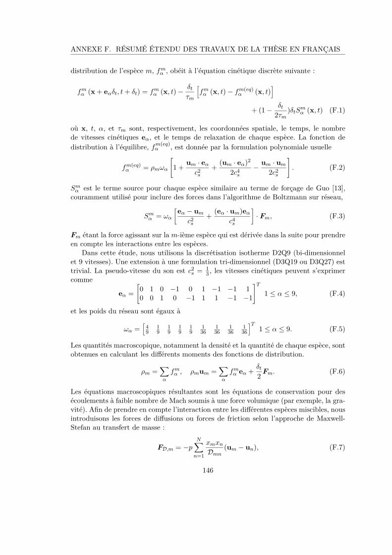
ANNEXE F. RÉSUMÉ ÉTENDU DES TRAVAUX DE LA THÈSE EN FRANÇAIS
distribution de l’espèce m, fmα , obéit à l’équation cinétique discrète suivante :
fmα (x + eαδt, t+ δt) = fm
α (x, t) − δt
τm
[fm
α (x, t) − fm(eq)α (x, t)
]+ (1 − δt
2τm)δtS
mα (x, t) (F.1)
où x, t, α, et τm sont, respectivement, les coordonnées spatiale, le temps, le nombrede vitesses cinétiques eα, et le temps de relaxation de chaque espèce. La fonction dedistribution à l’équilibre, fm(eq)
α , est donnée par la formulation polynomiale usuelle
fm(eq)α = ρmωα
[1 + um · eα
c2s
+ (um · eα)2
2c4s
− um · um
2c2s
]. (F.2)
Smα est le terme source pour chaque espèce similaire au terme de forçage de Guo [13],
couramment utilisé pour inclure des forces dans l’algorithme de Boltzmann sur réseau,
Smα = ωα
[eα − um
c2s
+ (eα · um)eα
c4s
]· Fm, (F.3)
Fm étant la force agissant sur la m-ième espèce qui est dérivée dans la suite pour prendreen compte les interactions entre les espèces.
Dans cette étude, nous utilisons la discrétisation isotherme D2Q9 (bi-dimensionnelet 9 vitesses). Une extension à une formulation tri-dimensionnel (D3Q19 ou D3Q27) esttrivial. La pseudo-vitesse du son est c2
s = 13 , les vitesses cinétiques peuvent s’exprimer
comme
eα =[0 1 0 −1 0 1 −1 −1 10 0 1 0 −1 1 1 −1 −1
]T
1 ≤ α ≤ 9, (F.4)
et les poids du réseau sont égaux à
ωα =[
49
19
19
19
19
136
136
136
136
]T1 ≤ α ≤ 9. (F.5)
Les quantités macroscopique, notamment la densité et la quantité de chaque espèce, sontobtenues en calculant les différents moments des fonctions de distribution.
ρm =∑
α
fmα , ρmum =
∑α
fmα eα + δt
2 Fm. (F.6)
Les équations macroscopiques résultantes sont les équations de conservation pour desécoulements à faible nombre de Mach soumis à une force volumique (par exemple, la gra-vité). Afin de prendre en compte l’interaction entre les différentes espèces miscibles, nousintroduisons les forces de diffusions ou forces de friction selon l’approche de Maxwell-Stefan au transfert de masse :
FD,m = −pN∑
n=1
xmxn
Dmn(um − un), (F.7)
146

ANNEXE F. RÉSUMÉ ÉTENDU DES TRAVAUX DE LA THÈSE EN FRANÇAIS
et Fm devientFm = FD,m + FB,m, (F.8)
où FB,m est une force volumique. Ainsi les équations cinétiques discrètes (F.1) pour lesdifférentes espèces sont couplées par l’intermédiaire de Fm. Puisque les force de diffusionFD,m dépendent de la vitesse, de la pression totale p, des fraction molaires xm, et descoefficients de diffusion (Maxwell-Stefan) Dmn, un système linéaire doit être résolu àchaque pas de temps afin de calculer la quantité de mouvement de chaque espèce grâce àl’équation (F.6). Cette force également appelée force de friction intermoléculaire dépendde la vitesse relative de chaque espèce. Ainsi, lorsque toutes les espèces ont la mêmevitesse, il n’y a pas de diffusion. Notons que la force de friction intramoléculaire liée à laviscosité est déjà pris en compte par l’opérateur de collision BGK de manière similaire aucas des écoulements mono-espèce. L’idée d’inclure les effets de diffusion comme une forceagissant sur les molécules date des premiers travaux de la théorie cinétique des gaz parMaxwell [38]. La même expression a été rigoureusement dérivée plus tard par Chapmanet Cowling [2], une discussion détaillée est donnée par Hirschfelder, Curtiss, et Bird [1]et Kerkhof et Geboers présentent une dérivation plus récente dans la référence [59]. Delongs et compliqués développements mathématiques sont nécessaires pour obtenir cetteforce de friction intermoléculaire à partir de la théorie cinétique des gaz, elle ne doncpas présenté. Les principales étapes de la dérivation font appel au développement deChapman et Enskog, à la linéarisation, de l’intégrale de collision (1.10) et à sa solutionapprochée par l’intermédiaire d’un développement en série des vitesses à partir des po-lynômes de Sonine (ou Laguerre) et non d’Hermite. Une méthode équivalente utilisantles polynômes d’Hermite, les équations des treize moments de Grad, a été proposée parZhdanov [60].
Conclusion
La première partie de cette thèse couvre les fondamentaux de la méthode de Boltz-mann sur réseau. Partant de la théorie cinétique des gaz et de l’équation de Boltzmann,une formulation discrète est proposé. Un outil majeur pour obtenir les équations macro-scopiques en jeu est le développement de Chapman et Enskog. Le temps de relaxationest ainsi lié à la dissipation visqueuse. Indépendamment, nous introduisons l’approcheproposée par Maxwell et Stefan pour modéliser la diffusion pure entre les espèces. Cetteapproche est plus commode et possède une interprétation plus physique dans le cas detrois ou plus espèces comparée à la formulation de Fick traditionnelle. De plus, nousmettons en avant les effets non-triviaux de diffusion multi-espèces qui peuvent appa-raître lors de la diffusion de trois ou plus composants tel que la diffusion osmotique, ladiffusion inverse et la barrière de diffusion. La contribution fondamentale de cette thèseest de combiner ces idées et de proposer une méthode de Boltzmann sur réseau pour lesgaz miscibles dans la seconde partie de la thèse.
Différentes méthodes de Boltzmann sur réseau pour les écoulements multi-espècesexistent déjà. Il n’y a pas un unique ou communément admis opérateur de collision de
147

ANNEXE F. RÉSUMÉ ÉTENDU DES TRAVAUX DE LA THÈSE EN FRANÇAIS
type BGK, chaque modèle dépend de la théorie cinétique sous-jacente choisie. Cepen-dant, pour tout les modèles dans le cas d’un mélange binaire, la variation de la quantitéde mouvement induite par la collision a une forme similaire à la force intermoléculairede friction, c’est à dire un coefficient multiplié par la différence de vitesse des deux es-pèces. Les précédents modèles nécessitent de fortement modifier l’étape de collision parrapport à la formulation standard afin de prendre en compte l’interaction entre les com-posants. L’algorithme est alors plus complexe, coûteux en temps de calcul, et par dessustout, ne peut être facilement implémenter dans des codes existant. Le point central dela méthode de Boltzmann sur réseau est la collision, la modifier signifie généralementréécrire entièrement le code. Dans l’approche proposée, l’équilibre usuel est utilisé com-biné avec la force de friction intermoléculaire. Beaucoup moins d’effort est alors requispour transformer un code mono-espèce pour qu’il prenne en compte la diffusion entre demultiple espèces. La dissipation visqueuse est liée à la relaxation vers l’état d’équilibretandis que la diffusion moléculaire est associée avec la force de friction intermoléculaire.Le calcul des coefficients de transport est possible à l’aide de la cinétique des gaz. Enplus du coefficient de diffusion (Maxwell-Stefan), une viscosité partielle est égalementdéfinie pour chaque composant. Le problème de la vitesse du son fixé par le réseau estpropre à la méthode de Boltzmann sur réseau. Ce problème est évité en utilisant uneforce artificielle pour modifier l’équation d’état de chaque espèce en fonction de sa massemoléculaire. Les résultats obtenus sont en excellent accord avec des solutions analytiques,expérimentales, et numériques. La dynamique complexe de diffusion de trois espèces ouplus est retrouvée, et le modèle proposé est capable de simuler les phénomènes de dif-fusion osmotique, de diffusion inverse, et de barrière de diffusion. Après avoir validé lescaractéristiques de notre modèle, nous l’appliquons à l’instabilité de digitation visqueuseet discutons des résultats obtenus dans la dernière partie de la thèse.
L’instabilité de digitation visqueuse est simulée en considérant dans un milieu poreuxdeux espèces dans des proportions différentes soit un mélange moins visqueux déplaçantun mélange plus visqueux. Les principaux moteurs de l’instabilité sont la diffusion etle contraste de viscosité entre les espèces. Deux stratégies sont envisagées pour simulerles effets d’un milieu poreux. Les méthodes de rebond partiel et de force de Brinkmanbien que basées sur des approches fondamentalement différentes donnent dans notre casdes résultats identiques. Les taux de croissance de l’instabilité calculés à partir de lasimulation coïncident avec ceux obtenus à partir d’analyses de stabilité linéaire. L’évo-lution de la longueur de mélange peut être divisée en deux étapes dominées d’abord parla diffusion puis par la convection. La physique de la digitation visqueuse est ainsi cor-rectement simulée. Toutefois, les effets de diffusion multi-espèces ne sont généralementpas pris en compte lors de la digitation visqueuse de trois espèces et plus. Ces derniersne sont pas négligeable puisque nous mettons en avant une configuration initialementstable qui se déstabilise. La diffusion inverse entraîne la digitation dont l’impact dépendde la diffusion entre les espèces. Après avoir appliqué avec succès notre modèle au casde la digitation visqueuse, il nous tarde de nous nous attaquer à d’autres problèmesimpliquant des écoulements multi-espèces.
148

ANNEXE F. RÉSUMÉ ÉTENDU DES TRAVAUX DE LA THÈSE EN FRANÇAIS
PerspectivesLa dérivation du modèle proposé est rigoureusement exacte seulement pour les gaz
dilués. Nous pouvons, dans une certaine mesure, l’appliquer aux liquides et gaz généraux.Les équation de Maxwell-Stefan sont aussi valides pour les gaz de faible et grande densité,les liquides et les polymères. On peut supposer que la force de friction intermoléculaireest toujours adéquate pour décrire la diffusion moléculaire dans ces cas. La pressionpartielle n’est bien définie dans le cas des gaz non-idéaux et ses gradients doivent êteremplacés par les gradient du potentiel chimique. Les coefficients de transport doiventêtre calculés à partir de la théorie cinétique d’Eyring (liquides) ou d’Enskog (gaz denses)[1]. Des études plus fondamentales sont nécessaires pour approfondir notre modèle. Parexemple, la simulation d’une couche de mélange entre trois espèces pourrait mettre enavant des mécanismes intéressants. Une comparaison avec une expérience récente et biendocumentée serait bénéfique. Un point de départ pour mesurer l’influence des viscositéspartielles peut se baser sur les expériences d’écoulements de jets à viscosité variableeffectuées dans la référence [105].
Concernant les simulations de digitation visqueuse, d’autres configurations du mé-lange à trois espèces pourraient être considérées. Une étude paramétrique peut êtreenvisagée et prolongerait les premiers résultats obtenus ici. Une autre possibilité est demodéliser les pores à la place de simuler leur effets. Bien qu’étant plus coûteux, cette si-mulation soulignera les différentes échelles du milieu poreux en jeu. Finalement, on peutnoter que la force de friction du milieu poreux a une forme similaire à l’approximationde Boussinesq fait dans le cas des problèmes de double diffusion convection rencontrésdans les océans et cela ouvre de nouvelles perspectives pour le modèle proposé.
Les publications suivantes sont liées à ce travail (voir aussi l’annexe E) :— Lucien Vienne, et al. “Lattice Boltzmann method for miscible gases : A forcing-
term approach”. In : Physical Review E. [106]— Lucien Vienne, et al. “Viscous fingering simulation by the lattice Boltzmann me-
thod”. Under preparation.
149


Bibliography
151


Bibliography
[1] J. O. Hirschfelder, C. F. Curtiss et R. B. Bird. Molecular Theory of Gasesand Liquids. Second printing. John Wiley & Sons, 1964. isbn : 9780471400653(cf. p. 5, 11, 13, 16, 19, 45, 47, 62, 71, 72, 82, 116, 129, 130, 132, 145, 147, 149).
[2] S. Chapman et T. G. Cowling. The Mathematical Theory of Non-uniformGases. 3e éd. Cambridge University Press, 1970. isbn : 052140844X (cf. p. 13,29, 30, 62, 147).
[3] P. L. Bhatnagar, E. P. Gross et M. Krook. « A Model for Collision Processesin Gases. I. Small Amplitude Processes in Charged and Neutral One-ComponentSystems ». In : Phys. Rev. 94 (3 1954), p. 511–525. doi : 10.1103/PhysRev.94.511 (cf. p. 15, 58).
[4] Timm Krüger et al. The Lattice Boltzmann Method. Springer International Pu-blishing, 2017. doi : 10.1007/978-3-319-44649-3 (cf. p. 16, 21, 58).
[5] X. Shan, X. Yuan et H. Chen. « Kinetic theory representation of hydrodyna-mics : a way beyond the Navier-Stokes equation ». In : Journal of Fluid Mechanics550.-1 (fév. 2006), p. 413. doi : 10.1017/s0022112005008153 (cf. p. 19, 21, 24,123, 124).
[6] Sauro Succi. The Lattice Boltzmann Equation for Fluid Dynamics and Beyond.Oxford University Press, 2001. isbn : 978-0-19-850398-9 (cf. p. 20).
[7] Z. Chai et T. S. Zhao. « Lattice Boltzmann model for the convection-diffusionequation ». In : Physical Review E 87.6 (juin 2013). doi : 10.1103/physreve.87.063309 (cf. p. 20).
[8] Baochang Shi et Zhaoli Guo. « Lattice Boltzmann model for nonlinear convection-diffusion equations ». In : Physical Review E 79.1 (jan. 2009). doi : 10.1103/physreve.79.016701 (cf. p. 20).
[9] Hiroshi Otomo, Bruce M. Boghosian et François Dubois. « Two complemen-tary lattice-Boltzmann-based analyses for nonlinear systems ». In : Physica A :Statistical Mechanics and its Applications 486 (nov. 2017), p. 1000–1011. doi :10.1016/j.physa.2017.06.010 (cf. p. 20).
[10] Yan Guangwu. « A Lattice Boltzmann Equation for Waves ». In : Journal ofComputational Physics 161.1 (juin 2000), p. 61–69. doi : 10.1006/jcph.2000.6486 (cf. p. 20).
[11] Jian Guo Zhou. Lattice Boltzmann Methods for Shallow Water Flows. SpringerBerlin Heidelberg, 2004. doi : 10.1007/978-3-662-08276-8 (cf. p. 20).
[12] Harold Grad. « On the kinetic theory of rarefied gases ». In : Communicationson Pure and Applied Mathematics 2.4 (déc. 1949), p. 331–407. doi : 10.1002/cpa.3160020403 (cf. p. 21, 122).
[13] Zhaoli Guo, Chuguang Zheng et Baochang Shi. « Discrete lattice effects on theforcing term in the lattice Boltzmann method ». In : Phys. Rev. E 65 (4 avr.2002), p. 046308. doi : 10.1103/PhysRevE.65.046308 (cf. p. 28, 61, 64, 65, 146).
153

Bibliography
[14] Michael Junk, Axel Klar et Li-Shi Luo. « Asymptotic analysis of the latticeBoltzmann equation ». In : Journal of Computational Physics 210.2 (déc. 2005),p. 676–704. doi : 10.1016/j.jcp.2005.05.003 (cf. p. 34).
[15] François Dubois. « Equivalent partial differential equations of a lattice Boltz-mann scheme ». In : Computers & Mathematics with Applications 55.7 (avr. 2008),p. 1441–1449. doi : 10.1016/j.camwa.2007.08.003 (cf. p. 34).
[16] Wen-An Yong, Weifeng Zhao et Li-Shi Luo. « Theory of the Lattice Boltzmannmethod : Derivation of macroscopic equations via the Maxwell iteration ». In :Physical Review E 93.3 (mar. 2016). doi : 10.1103/physreve.93.033310 (cf.p. 34).
[17] Simon Marié, Denis Ricot et Pierre Sagaut. « Comparison between latticeBoltzmann method and Navier–Stokes high order schemes for computational ae-roacoustics ». In : Journal of Computational Physics 228.4 (mar. 2009), p. 1056–1070. doi : 10.1016/j.jcp.2008.10.021 (cf. p. 34).
[18] Gauthier Wissocq, Pierre Sagaut et Jean-François Boussuge. « An extendedspectral analysis of the lattice Boltzmann method : modal interactions and stabi-lity issues ». In : Journal of Computational Physics 380 (mar. 2019), p. 311–333.doi : 10.1016/j.jcp.2018.12.015 (cf. p. 34).
[19] Pierre Lallemand et Li-Shi Luo. « Theory of the lattice Boltzmann method :Dispersion, dissipation, isotropy, Galilean invariance, and stability ». In : PhysicalReview E 61.6 (juin 2000), p. 6546–6562. doi : 10.1103/physreve.61.6546 (cf.p. 36).
[20] Christophe Coreixas, Bastien Chopard et Jonas Latt. « Comprehensive com-parison of collision models in the lattice Boltzmann framework : Theoretical inves-tigations ». In : Physical Review E 100.3 (sept. 2019). doi : 10.1103/physreve.100.033305 (cf. p. 36, 39).
[21] P. V. Coveney et al. « Multiple relaxation time lattice Boltzmann models inthree dimensions ». In : Philosophical Transactions of the Royal Society of Lon-don. Series A : Mathematical, Physical and Engineering Sciences 360.1792 (2002),p. 437–451. doi : 10.1098/rsta.2001.0955 (cf. p. 37, 61, 145).
[22] Dominique d’Humières et Irina Ginzburg. « Viscosity independent numericalerrors for Lattice Boltzmann models : From recurrence equations to “magic”collision numbers ». In : Computers & Mathematics with Applications 58.5 (sept.2009), p. 823–840. doi : 10.1016/j.camwa.2009.02.008 (cf. p. 37, 94).
[23] L. Talon et al. « Assessment of the two relaxation time Lattice-Boltzmannscheme to simulate Stokes flow in porous media ». In : Water Resources Research48.4 (avr. 2012). doi : 10.1029/2011wr011385 (cf. p. 37, 94).
[24] Siarhei Khirevich, Irina Ginzburg et Ulrich Tallarek. « Coarse- and fine-grid numerical behavior of MRT/TRT lattice-Boltzmann schemes in regular andrandom sphere packings ». In : Journal of Computational Physics 281 (jan. 2015),p. 708–742. doi : 10.1016/j.jcp.2014.10.038 (cf. p. 37, 94).
154
Bibliography
[25] Maxime Février. « Extension et analyse des schémas de Boltzmann sur réseau :les schémas à vitesse relative. » Thèse de doct. 2015 (cf. p. 37).
[26] Alessandro De Rosis et Kai H. Luo. « Role of higher-order Hermite polyno-mials in the central-moments-based lattice Boltzmann framework ». In : PhysicalReview E 99.1 (jan. 2019). doi : 10.1103/physreve.99.013301 (cf. p. 37).
[27] Martin Geier et al. « The cumulant lattice Boltzmann equation in three dimen-sions : Theory and validation ». In : Computers & Mathematics with Applications70.4 (août 2015), p. 507–547. doi : 10.1016/j.camwa.2015.05.001 (cf. p. 37,61, 145).
[28] Jonas Latt et Bastien Chopard. « Lattice Boltzmann method with regularizedpre-collision distribution functions ». In : Mathematics and Computers in Simu-lation 72.2-6 (sept. 2006), p. 165–168. doi : 10.1016/j.matcom.2006.05.017(cf. p. 38, 61, 145).
[29] Orestis Malaspinas. « Increasing stability and accuracy of the latticeBoltzmannscheme : recursivity and regularization ». In : arXiv e-prints, arXiv :1505.06900(mai 2015), arXiv :1505.06900. arXiv : 1505 . 06900 [physics.flu-dyn] (cf.p. 38).
[30] Christophe Coreixas. « High-order extension of the recursive regularized latticeBoltzmann method ». Thèse de doct. 2018 (cf. p. 38).
[31] S. S. Chikatamarla, S. Ansumali et I. V. Karlin. « Entropic Lattice Boltz-mann Models for Hydrodynamics in Three Dimensions ». In : Phys. Rev. Lett. 97(1 juil. 2006), p. 010201. doi : 10.1103/PhysRevLett.97.010201 (cf. p. 39, 61,145).
[32] Qisu Zou et Xiaoyi He. « On pressure and velocity boundary conditions for thelattice Boltzmann BGK model ». In : Physics of Fluids 9.6 (juin 1997), p. 1591–1598. doi : 10.1063/1.869307 (cf. p. 42).
[33] C. F. Curtiss et R. Byron Bird. « Multicomponent Diffusion ». In : Industrial &Engineering Chemistry Research 38.7 (juil. 1999), p. 2515–2522. doi : 10.1021/ie9901123 (cf. p. 45).
[34] Charles F. Curtiss et Joseph O. Hirschfelder. « Transport Properties of Mul-ticomponent Gas Mixtures ». In : The Journal of Chemical Physics 17.6 (juin1949), p. 550–555. doi : 10.1063/1.1747319 (cf. p. 45, 47, 62, 71).
[35] Forman A. Williams. Combustion Theory. 2e éd. Benjamin/Cummings Pub. Co,1985. isbn : 0805398015 (cf. p. 45).
[36] Ingo Müller. « A thermodynamic theory of mixtures of fluids ». In : Archivefor Rational Mechanics and Analysis 28.1 (jan. 1968), p. 1–39. doi : 10.1007/bf00281561 (cf. p. 45).
[37] R. Taylor et R. Krishna. Multicomponent Mass Transfer. John Wiley & Sons,1993. isbn : 9780471574170 (cf. p. 45, 47, 51, 80).
155

Bibliography
[38] James Clerk Maxwell. « IV. On the dynamical theory of gases ». In : Philoso-phical Transactions of the Royal Society of London 157 (1867), p. 49–88. doi :10.1098/rstl.1867.0004 (cf. p. 47, 62, 147).
[39] J. Stefan. « Über die Theorie der Eisbildung ». In : Monatshefte für Mathematikund Physik 1.1 (déc. 1890), p. 1–6. doi : 10.1007/bf01692459 (cf. p. 47).
[40] R. Krishna et J.A. Wesselingh. « The Maxwell-Stefan approach to mass trans-fer ». In : Chemical Engineering Science 52.6 (mar. 1997), p. 861–911. doi :10.1016/s0009-2509(96)00458-7 (cf. p. 47).
[41] J. B. Duncan et H. L. Toor. « An experimental study of three component gasdiffusion ». In : AIChE Journal 8.1 (mar. 1962), p. 38–41. doi : 10.1002/aic.690080112 (cf. p. 48, 78).
[42] S. A. Hosseini, N. Darabiha et D. Thévenin. « Mass-conserving advection–diffusionLattice Boltzmann model for multi-species reacting flows ». In : Physica A : Sta-tistical Mechanics and its Applications 499 (2018), p. 40–57. doi : 10.1016/j.physa.2018.01.034 (cf. p. 57).
[43] Li-Shi Luo et Sharath S. Girimaji. « Theory of the lattice Boltzmann method :Two-fluid model for binary mixtures ». In : Phys. Rev. E 67 (3 mar. 2003),p. 036302. doi : 10.1103/PhysRevE.67.036302 (cf. p. 58, 71).
[44] Lawrence Sirovich. « Kinetic Modeling of Gas Mixtures ». In : Physics of Fluids5.8 (1962), p. 908. doi : 10.1063/1.1706706 (cf. p. 58).
[45] Abhijit S. Joshi et al. « Lattice Boltzmann method for continuum, multi-componentmass diffusion in complex 2D geometries ». In : Journal of Physics D : AppliedPhysics 40.9 (avr. 2007), p. 2961–2971. doi : 10.1088/0022-3727/40/9/044(cf. p. 58).
[46] Zi-Xiang Tong et al. « A multi-component lattice Boltzmann method in consistentwith Stefan–Maxwell equations : Derivation, validation and application in po-rous medium ». In : Computers & Fluids 105 (déc. 2014), p. 155–165. doi :10.1016/j.compfluid.2014.09.022 (cf. p. 58, 71).
[47] Pietro Asinari. « Semi-implicit-linearized multiple-relaxation-time formulationof lattice Boltzmann schemes for mixture modeling ». In : Phys. Rev. E 73 (5mai 2006), p. 056705. doi : 10.1103/PhysRevE.73.056705 (cf. p. 58, 71).
[48] Pietro Asinari et Li-Shi Luo. « A consistent lattice Boltzmann equation withbaroclinic coupling for mixtures ». In : Journal of Computational Physics 227.8(avr. 2008), p. 3878–3895. doi : 10.1016/j.jcp.2007.12.001 (cf. p. 58, 71).
[49] Bernard B. Hamel. « Kinetic Model for Binary Gas Mixtures ». In : Physics ofFluids 8.3 (1965), p. 418. doi : 10.1063/1.1761239 (cf. p. 58).
[50] Victor Sofonea et Robert F. Sekerka. « BGK models for diffusion in isothermalbinary fluid systems ». In : Physica A : Statistical Mechanics and its Applications299.3-4 (oct. 2001), p. 494–520. doi : 10.1016/s0378-4371(01)00246-1 (cf.p. 58).
156

Bibliography
[51] S. Arcidiacono et al. « Lattice Boltzmann model for the simulation of mul-ticomponent mixtures ». In : Phys. Rev. E 76 (4 oct. 2007), p. 046703. doi :10.1103/PhysRevE.76.046703 (cf. p. 58, 71, 80, 81, 82).
[52] Jinfen Kang, Nikolaos I. Prasianakis et John Mantzaras. « Thermal multi-component lattice Boltzmann model for catalytic reactive flows ». In : Phys. Rev.E 89 (6 juin 2014), p. 063310. doi : 10.1103/PhysRevE.89.063310 (cf. p. 58,71, 75).
[53] Pietro Asinari. « Multiple-relaxation-time lattice Boltzmann scheme for homo-geneous mixture flows with external force ». In : Phys. Rev. E 77 (5 mai 2008),p. 056706. doi : 10.1103/PhysRevE.77.056706 (cf. p. 58, 71).
[54] Pierre Andries, Kazuo Aoki et Benoit Perthame. « A Consistent BGK-TypeModel for Gas Mixtures ». In : Journal of Statistical Physics 106.5/6 (2002),p. 993–1018. doi : 10.1023/a:1014033703134 (cf. p. 58).
[55] P. Asinari. « Lattice Boltzmann scheme for mixture modeling : Analysis of thecontinuum diffusion regimes recovering Maxwell-Stefan model and incompressibleNavier-Stokes equations ». In : Physical Review E 80 (5 2009), p. 056701. doi :10.1103/PhysRevE.80.056701 (cf. p. 58, 71).
[56] Sam Bennett, Pietro Asinari et Paul J. Dellar. « A lattice Boltzmann modelfor diffusion of binary gas mixtures that includes diffusion slip ». In : InternationalJournal for Numerical Methods in Fluids 69.1 (mar. 2011), p. 171–189. doi :10.1002/fld.2549 (cf. p. 58).
[57] Jens Zudrop et al. « A robust lattice Boltzmann method for parallel simulationsof multicomponent flows in complex geometries ». In : Computers & Fluids 153(août 2017), p. 20–33. doi : 10.1016/j.compfluid.2017.04.021 (cf. p. 58, 71).
[58] Jens Zudrop, Sabine Roller et Pietro Asinari. « Lattice Boltzmann schemefor electrolytes by an extended Maxwell-Stefan approach ». In : Phys. Rev. E 89(5 mai 2014), p. 053310. doi : 10.1103/PhysRevE.89.053310 (cf. p. 58).
[59] Piet J. A. M. Kerkhof et Marcel A. M. Geboers. « Toward a unified theoryof isotropic molecular transport phenomena ». In : AIChE Journal 51.1 (2004),p. 79–121. doi : 10.1002/aic.10309 (cf. p. 62, 71, 129, 132, 147).
[60] V Zhdanov, Yu Kagan et A Sazykin. « Effect of viscous transfer of momentumon diffusion in a gas mixture ». In : Sov. Phys. JETP 15 (1962), p. 596–602 (cf.p. 63, 147).
[61] Michael E. McCracken et John Abraham. « Lattice Boltzmann methods forbinary mixtures with different molecular weights ». In : Phys. Rev. E 71 (4 avr.2005), p. 046704. doi : 10.1103/PhysRevE.71.046704 (cf. p. 63).
[62] N. Looije et al. « Introducing a variable speed of sound in single-componentlattice Boltzmann simulations of isothermal fluid flows ». In : Computers & Fluids167 (mai 2018), p. 129–145. doi : 10.1016/j.compfluid.2018.02.037 (cf. p. 63,73, 75).
157

Bibliography
[63] J M Buick et J A Cosgrove. « Investigation of a lattice Boltzmann model witha variable speed of sound ». In : Journal of Physics A : Mathematical and General39.44 (oct. 2006), p. 13807–13815. doi : 10.1088/0305-4470/39/44/013 (cf.p. 64).
[64] Daniel D. Joseph et Yuriko Y. Renardy. Fluid Dynamics of Two Miscible Li-quids with Diffusion and Gradient Stresses. Springer New York, 1993, p. 324–395.doi : 10.1007/978-1-4615-7061-5_6 (cf. p. 67).
[65] Daniel D. Joseph, Adam Huang et Howard Hu. « Non-solenoidal velocity effectsand Korteweg stresses in simple mixtures of incompressible liquids ». In : PhysicaD : Nonlinear Phenomena 97.1-3 (oct. 1996), p. 104–125. doi : 10.1016/0167-2789(96)00097-8 (cf. p. 67).
[66] C. R. Wilke. « A Viscosity Equation for Gas Mixtures ». In : The Journal ofChemical Physics 18.4 (avr. 1950), p. 517–519. doi : 10.1063/1.1747673 (cf.p. 72, 130, 131, 132).
[67] K. R. Arnold et H. L. Toor. « Unsteady diffusion in ternary gas mixtures ».In : AIChE Journal 13.5 (sept. 1967), p. 909–914. doi : 10.1002/aic.690130518(cf. p. 78).
[68] Rajamani Krishna. « Uphill diffusion in multicomponent mixtures ». In : Che-mical Society Reviews 44.10 (2015), p. 2812–2836. doi : 10.1039/c4cs00440j(cf. p. 80).
[69] G M Homsy. « Viscous Fingering in Porous Media ». In : Annual Review of FluidMechanics 19.1 (jan. 1987), p. 271–311. doi : 10.1146/annurev.fl.19.010187.001415 (cf. p. 89, 90, 100, 104, 106).
[70] Japinder S. Nijjer, Duncan R. Hewitt et Jerome A. Neufeld. « The dynamicsof miscible viscous fingering from onset to shutdown ». In : Journal of FluidMechanics 837 (jan. 2018), p. 520–545. doi : 10.1017/jfm.2017.829 (cf. p. 89,91, 100, 104).
[71] S. Hill et F.Inst. P. « Channeling in packed columns ». In : Chemical EngineeringScience 1.6 (1952), p. 247–253. doi : 10.1016/0009-2509(52)87017-4 (cf. p. 90).
[72] Philip Geoffrey Saffman et Geoffrey Ingram Taylor. « The penetration of afluid into a porous medium or Hele-Shaw cell containing a more viscous liquid ».In : Proceedings of the Royal Society of London. Series A. Mathematical andPhysical Sciences 245.1242 (juin 1958), p. 312–329. doi : 10.1098/rspa.1958.0085 (cf. p. 90).
[73] C. T. Tan et G. M. Homsy. « Stability of miscible displacements in porousmedia : Rectilinear flow ». In : Physics of Fluids 29.11 (1986), p. 3549. doi :10.1063/1.865832 (cf. p. 91, 100, 101, 106).
158
Bibliography
[74] Satyajit Pramanik et Manoranjan Mishra. « Effect of Péclet number on mis-cible rectilinear displacement in a Hele-Shaw cell ». In : Physical Review E 91.3(mar. 2015). doi : 10.1103/physreve.91.033006 (cf. p. 91, 95, 98, 100, 101,102, 106).
[75] Tapan Kumar Hota, Satyajit Pramanik et Manoranjan Mishra. « Nonmodallinear stability analysis of miscible viscous fingering in porous media ». In : Phy-sical Review E 92.5 (nov. 2015). doi : 10.1103/physreve.92.053007 (cf. p. 91,100, 101).
[76] W. B. Zimmerman et G. M. Homsy. « Three-dimensional viscous fingering : Anumerical study ». In : Physics of Fluids A : Fluid Dynamics 4.9 (sept. 1992),p. 1901–1914. doi : 10.1063/1.858361 (cf. p. 91, 97).
[77] A. Riaz et E. Meiburg. « Three-dimensional miscible displacement simulationsin homogeneous porous media with gravity override ». In : Journal of Fluid Me-chanics 494 (nov. 2003), p. 95–117. doi : 10.1017/s0022112003005974 (cf. p. 91,97).
[78] Birendra Jha, Luis Cueto-Felgueroso et Ruben Juanes. « Quantifying mixingin viscously unstable porous media flows ». In : Physical Review E 84.6 (déc.2011). doi : 10.1103/physreve.84.066312 (cf. p. 91).
[79] Richard Holme et Daniel H. Rothman. « Lattice-gas and lattice-Boltzmannmodels of miscible fluids ». In : Journal of Statistical Physics 68.3-4 (août 1992),p. 409–429. doi : 10.1007/bf01341756 (cf. p. 91).
[80] N. Rakotomalala, D. Salin et P. Watzky. « Miscible displacement betweentwo parallel plates : BGK lattice gas simulations ». In : Journal of Fluid Mechanics338 (mai 1997), p. 277–297. doi : 10.1017/s0022112097004928 (cf. p. 91, 94).
[81] Stuart D.C. Walsh, Holly Burwinkle et Martin O. Saar. « A new partial-bounceback lattice Boltzmann method for fluid flow through heterogeneous me-dia ». In : Computers & Geosciences 35.6 (juin 2009), p. 1186–1193. doi : 10.1016/j.cageo.2008.05.004 (cf. p. 93).
[82] Jiujiang Zhu et Jingsheng Ma. « An improved gray lattice Boltzmann modelfor simulating fluid flow in multi-scale porous media ». In : Advances in WaterResources 56 (juin 2013), p. 61–76. doi : 10.1016/j.advwatres.2013.03.001(cf. p. 93).
[83] Hiroaki Yoshida et Hidemitsu Hayashi. « Transmission–Reflection Coefficientin the Lattice Boltzmann Method ». In : Journal of Statistical Physics 155.2 (fév.2014), p. 277–299. doi : 10.1007/s10955-014-0953-7 (cf. p. 93, 94).
[84] D.T. Thorne et M.C. Sukop. « Lattice Boltzmann model for the elder pro-blem ». In : Computational Methods in Water Resources : Volume 2, Proceedingsof the XVth International Conference on Computational Methods in Water Re-sources. Elsevier, 2004, p. 1549–1557. doi : 10.1016/s0167-5648(04)80165-5(cf. p. 93).
159
Bibliography
[85] Chen Chen et al. « Chapman–Enskog Analyses on the Gray Lattice BoltzmannEquation Method for Fluid Flow in Porous Media ». In : Journal of StatisticalPhysics 171.3 (mar. 2018), p. 493–520. doi : 10.1007/s10955- 018- 2005- 1(cf. p. 93, 94).
[86] Irina Ginzburg. « Consistent lattice Boltzmann schemes for the Brinkman modelof porous flow and infinite Chapman-Enskog expansion ». In : Physical Review E77.6 (juin 2008). doi : 10.1103/physreve.77.066704 (cf. p. 94).
[87] Zhaoli Guo et T. S. Zhao. « Lattice Boltzmann model for incompressible flowsthrough porous media ». In : Physical Review E 66.3 (sept. 2002). doi : 10.1103/physreve.66.036304 (cf. p. 94).
[88] Nicos S. Martys. « Improved approximation of the Brinkman equation using alattice Boltzmann method ». In : Physics of Fluids 13.6 (juin 2001), p. 1807–1810.doi : 10.1063/1.1368846 (cf. p. 94).
[89] Michael A. A. Spaid et Frederick R. Phelan. « Lattice Boltzmann methods formodeling microscale flow in fibrous porous media ». In : Physics of Fluids 9.9(sept. 1997), p. 2468–2474. doi : 10.1063/1.869392 (cf. p. 94).
[90] Patrick Grosfils et al. « Structural and dynamical characterization of Hele–Shawviscous fingering ». In : Philosophical Transactions of the Royal Society of Lon-don. Series A : Mathematical, Physical and Engineering Sciences 362.1821 (août2004). Sous la dir. de M. Al–Ghoul, J. P. Boon et P. V. Coveney, p. 1723–1734. doi : 10.1098/rsta.2004.1398 (cf. p. 94).
[91] Irina Ginzburg. « Comment on An improved gray Lattice Boltzmann model forsimulating fluid flow in multi-scale porous media : Intrinsic links between LBEBrinkman schemes ». In : Advances in Water Resources 88 (fév. 2016), p. 241–249. doi : 10.1016/j.advwatres.2014.05.007 (cf. p. 94).
[92] M. Norouzi et M. R. Shoghi. « A numerical study on miscible viscous fingeringinstability in anisotropic porous media ». In : Physics of Fluids 26.8 (août 2014),p. 084102. doi : 10.1063/1.4891228 (cf. p. 97, 100).
[93] M’hamed Bouzidi et al. « Lattice Boltzmann Equation on a Two-DimensionalRectangular Grid ». In : Journal of Computational Physics 172.2 (sept. 2001),p. 704–717. doi : 10.1006/jcph.2001.6850 (cf. p. 99).
[94] L. A. Hegele Jr, K. Mattila et P. C. Philippi. « Rectangular Lattice-BoltzmannSchemes with BGK-Collision Operator ». In : Journal of Scientific Computing56.2 (déc. 2012), p. 230–242. doi : 10.1007/s10915-012-9672-x (cf. p. 99).
[95] Cheng Peng et al. « A hydrodynamically-consistent MRT lattice Boltzmann mo-del on a 2D rectangular grid ». In : Journal of Computational Physics 326 (déc.2016), p. 893–912. doi : 10.1016/j.jcp.2016.09.031 (cf. p. 99).
160

Bibliography
[96] E. Vergnault, O. Malaspinas et P. Sagaut. « A lattice Boltzmann methodfor nonlinear disturbances around an arbitrary base flow ». In : Journal of Com-putational Physics 231.24 (oct. 2012), p. 8070–8082. doi : 10.1016/j.jcp.2012.07.021 (cf. p. 100).
[97] José Miguel Pérez, Alfonso Aguilar et Vassilis Theofilis. « Lattice Boltzmannmethods for global linear instability analysis ». In : Theoretical and ComputationalFluid Dynamics 31.5-6 (nov. 2016), p. 643–664. doi : 10.1007/s00162-016-0416-7 (cf. p. 100).
[98] O. Manickam et G. M. Homsy. « Stability of miscible displacements in porousmedia with nonmonotonic viscosity profiles ». In : Physics of Fluids A : FluidDynamics 5.6 (juin 1993), p. 1356–1367. doi : 10.1063/1.858571 (cf. p. 106).
[99] O. Manickam et G. M. Homsy. « Simulation of viscous fingering in miscibledisplacements with nonmonotonic viscosity profiles ». In : Physics of Fluids 6.1(jan. 1994), p. 95–107. doi : 10.1063/1.868049 (cf. p. 106).
[100] M. Mishra, M. Martin et A. De Wit. « Differences in miscible viscous fingeringof finite width slices with positive or negative log-mobility ratio ». In : PhysicalReview E 78.6 (déc. 2008). doi : 10.1103/physreve.78.066306 (cf. p. 106).
[101] S. H. Hejazi et al. « Viscous fingering of a miscible reactive A + B → C interface :a linear stability analysis ». In : Journal of Fluid Mechanics 652 (avr. 2010),p. 501–528. doi : 10.1017/s0022112010000327 (cf. p. 106).
[102] Y. Nagatsu et A. De Wit. « Viscous fingering of a miscible reactive A+B→Cinterface for an infinitely fast chemical reaction : Nonlinear simulations ». In :Physics of Fluids 23.4 (avr. 2011), p. 043103. doi : 10.1063/1.3567176 (cf.p. 106).
[103] L. A. Riolfo et al. « Experimental evidence of reaction-driven miscible viscousfingering ». In : Physical Review E 85.1 (jan. 2012). doi : 10.1103/physreve.85.015304 (cf. p. 106).
[104] V. Loodts et al. « Density profiles around A+B→C reaction-diffusion fronts inpartially miscible systems : A general classification ». In : Physical Review E 94.4(oct. 2016). doi : 10.1103/physreve.94.043115 (cf. p. 106).
[105] Benoît Talbot. « Mélange et dynamique de la turbulence en écoulements libresà viscosité variable. » Thèse de doct. 2009 (cf. p. 116, 149).
[106] Lucien Vienne, Simon Marié et Francesco Grasso. « Lattice Boltzmann me-thod for miscible gases : A forcing-term approach ». In : Physical Review E 100.2(août 2019). doi : 10.1103/physreve.100.023309 (cf. p. 116, 149).
[107] Harold Grad. « Note on N-dimensional Hermite polynomials ». In : Commu-nications on Pure and Applied Mathematics 2.4 (déc. 1949), p. 325–330. doi :10.1002/cpa.3160020402 (cf. p. 122).
[108] Bruce E Poling, John P O’Connell et J M Prausnitz. The properties of gasesand liquids. 5e éd. McGraw-Hill, 2000. isbn : 9780070116825 (cf. p. 129, 132).
161

Bibliography
[109] J. W. Buddenberg et C. R. Wilke. « Calculation of Gas Mixture Viscosities. »In : Industrial & Engineering Chemistry 41.7 (juil. 1949), p. 1345–1347. doi :10.1021/ie50475a011 (cf. p. 131).
[110] Lucien Vienne, Simon Marié et Francesco Grasso. « Simulation of ViscousFingering Instability by the Lattice Boltzmann Method ». In : AIAA Aviation2019 Forum. American Institute of Aeronautics et Astronautics, juin 2019. doi :10.2514/6.2019-3432 (cf. p. 137).
[111] B. Dorschner et al. « Grad’s approximation for moving and stationary walls inentropic lattice Boltzmann simulations ». In : Journal of Computational Physics295 (août 2015), p. 340–354. doi : 10.1016/j.jcp.2015.04.017 (cf. p. 139).
162


Lucien VIENNE
Simulation of multi-component flows by the latticeBoltzmann method and application to the viscous
fingering instability
Résumé : La méthode de Boltzmann sur réseau est une formulation discrète particulière de l’équation de Boltz-mann. Depuis ses débuts, il y a trente ans, cette méthode a gagné une certaine popularité et elle est maintenantutilisée dans presque tous les problèmes habituellement rencontrés en mécanique des fluides notamment pour lesécoulements multi-espèces. Dans le cadre de ce travail, une force de friction intermoléculaire est introduite pourmodéliser les interactions entre les molécules de différent types causant principalement la diffusion entre les es-pèces. Les phénomènes de dissipation visqueuse (collision usuelle) et de diffusion moléculaire (force de frictionintermoléculaire) sont séparés et peuvent être ajustés indépendamment. Le principal avantage de cette stratégieest sa compatibilité avec des optimisations de la collision usuelle et les opérateurs de collision avancés. Adapter uncode mono-espèce pour aboutir à un code multi-espèces est aisé et demande beaucoup moins d’effort comparé auxprécédentes tentatives. De plus, il n’ y a pas d’approximation du mélange, chaque espèce a ses propres coefficientsde transport pouvant être calculés à l’aide de la théorie cinétique des gaz. En général, la diffusion et la convectionsont vus comme deux mécanismes séparés : l’un agissant sur la masse d’une espèce, l’autre sur la quantité de mou-vement du mélange. En utilisant une force de friction intermoléculaire, la diffusion et la convection sont coupléspar l’intermédiaire la quantité de mouvement de chaque espèce. Les mécanismes de diffusion et de convection sontintimement liés dans de nombreux phénomènes physique tel que la digitation visqueuse.L’instabilité de digitation visqueuse est simulée en considérant dans un milieu poreux deux espèces dans desproportions différentes soit un mélange moins visqueux déplaçant un mélange plus visqueux. Les principauxmoteurs de l’instabilité sont la diffusion et le contraste de viscosité entre les espèces. Deux stratégies sont envisagéespour simuler les effets d’un milieu poreux. Les méthodes de rebond partiel et de force de Brinkman bien quebasées sur des approches fondamentalement différentes donnent dans notre cas des résultats identiques. Les tauxde croissance de l’instabilité calculés à partir de la simulation coïncident avec ceux obtenus à partir d’analyses destabilité linéaire. L’évolution de la longueur de mélange peut être divisée en deux étapes dominées d’abord par ladiffusion puis par la convection. La physique de la digitation visqueuse est ainsi correctement simulée. Toutefois,les effets de diffusion multi-espèces ne sont généralement pas pris en compte lors de la digitation visqueuse de troisespèces et plus. Ces derniers ne sont pas négligeable puisque nous mettons en avant une configuration initialementstable qui se déstabilise. La diffusion inverse entraîne la digitation dont l’impact dépend de la diffusion entre lesespèces.
Mots clés : méthode de Boltzmann sur réseau, mécanique des fluides, écoulements multi-espèces, dynamique dumélange, instabilité de digitation visqueuse
Abstract: The lattice Boltzmann method (LBM) is a specific discrete formulation of the Boltzmann equation.Since its first premises, thirty years ago, this method has gained some popularity and is now applied to almost allstandard problems encountered in fluid mechanics including multi-component flows. In this work, we introduce theinter-molecular friction forces to take into account the interaction between molecules of different kinds resultingprimarily in diffusion between components. Viscous dissipation (standard collision) and molecular diffusion (inter-molecular friction forces) phenomena are split, and both can be tuned distinctively. The main advantage of thisstrategy is optimizations of the collision and advanced collision operators are readily compatible. Adapting anexisting code from single component to multiple miscible components is straightforward and required much lesseffort than the large modifications needed from previously available lattice Boltzmann models. Besides, thereis no mixture approximation: each species has its own transport coefficients, which can be calculated from thekinetic theory of gases. In general, diffusion and convection are dealt with two separate mechanisms: one actingrespectively on the species mass and the other acting on the mixture momentum. By employing an inter-molecularfriction force, the diffusion and convection are coupled through the species momentum. Diffusion and convectionmechanisms are closely related in several physical phenomena such as in the viscous fingering instability.A simulation of the viscous fingering instability is achieved by considering two species in different proportions in aporous medium: a less viscous mixture displacing a more viscous mixture. The core ingredients of the instabilityare the diffusion and the viscosity contrast between the components. Two strategies are investigated to mimicthe effects of the porous medium. The gray lattice Boltzmann and Brinkman force models, although based onfundamentally different approaches, give in our case equivalent results. For early times, comparisons with linearstability analyses agree well with the growth rate calculated from the simulations. For intermediate times, theevolution of the mixing length can be divided into two stages dominated first by diffusion then by convection,as found in the literature. The whole physics of the viscous fingering is thus accurately simulated. Nevertheless,multi-component diffusion effects are usually not taken into account in the case of viscous fingering with threeand more species. These effects are non-negligible as we showcase an initial stable configuration that becomesunstable. The reverse diffusion induces fingering whose impact depends on the diffusion between species.
Keywords: lattice Boltzmann method, fluid mechanics, multi-component flows, mixture dynamics, viscousfingering instability


![From Lattice Boltzmann Method to Lattice Boltzmann Flux … · From Lattice Boltzmann Method to Lattice Boltzmann Flux Solver Yan Wang 1, ... flows [8,13–15], compressible flows](https://img.pdfslide.us/doc/110x75/5cadf91b88c9938f4d8c0cd6/from-lattice-boltzmann-method-to-lattice-boltzmann-flux-from-lattice-boltzmann.jpg)