SIMULATION OF FLOW AND TRANSPORT PROCESSES IN A DISCRETE …

SIMULATION OF FLOW AND TRANSPORT PROCESSES IN ADISCRETE FRACTURE-MATRIX SYSTEM II. EFFICIENT AND

ACCURATE STREAMLINE APPROACH

H. HÆGLAND, A. ASSTEERAWATT, R. HELMIG, AND H. K. DAHLE

Abstract. Simulations of flow and transport in fractured porous rocks using a discretefracture model have gradually become more practical, as a consequence of increasedcomputer power and improved simulation and characterization techniques. Fractures ina discrete model are generally described with one dimension less than the surroundingmatrix, the so-called lower-dimensional approach. However, high numerical diffusion inthe transport simulation causes an increased computational demand due to the fine-gridrequirement. A streamline method for transport for a lower dimensional discrete fracturemodel (DFML) is proposed in this paper. By solving the mass conservation equation us-ing a vertex-centered finite volume scheme, a pressure field is obtained. Then, a fractureexpansion and a flux recovery method are carried out to determine new mass conser-vative fluxes on a hybrid grid of triangles and quadrilaterals, on which streamlines aretraced. Only the advective transport is assumed for the streamline method. The resultsof the streamline method are compared with a grid-based finite volume method usingtwo different fracture-matrix systems: simple systems (a single fracture or systemati-cally distributed fractures) and complex fracture-matrix systems. Significantly differenttransport behavior can be observed in the two types of systems. The numerical diffusionin the grid-based transport simulation smears out the heterogeneity effect (fast trans-port in the fractures and slow transport in the matrix) and delays the plume migration.Whereas, the purely advective transport without numerical diffusion in the streamlinemethod leads to faster transport.

1. Introduction

Simulations of flow and transport in fractured porous rocks using a discrete fracturemodel have gradually become more practical, as a consequence of increased computerpower and improved simulation and characterization techniques. In a discrete fracturemodel, fractures may either be discretized with the same dimension as the surround-ing matrix elements, the so-called equi-dimensional approach, or with one dimension lessthan the matrix, the so-called lower-dimensional approach. The comparison study of thetwo discretization approaches presented in Neunhauserer [19] revealed a number of localdifferences for the flow and transport, but and only minor differences globally. Suffi-cient accuracy of global solutions with reduction of the computational time have lead towide-spread application of the lower-dimensional approach, see e.g., [23, 17, 14, 16], andreferences therein.In advective dominated problems like transport in fracture-matrix systems, grid-basedmethods such as finite difference, finite element and finite volume methods all using theEulerian approach, suffer from numerical diffusion. High numerical diffusion in the trans-port simulation, as shown in the associated paper, gives rise to an increased computationalburden since a very fine grid is required. Streamline methods have become a viable al-ternative to traditional finite element or finite difference reservoir simulation during thelast decade ([15, 27]). The advantages of streamline simulation are lower computationaldemand and less numerical diffusion compared with a grid-based transport model. On

1

2 H. HÆGLAND, A. ASSTEERAWATT, R. HELMIG, AND H. K. DAHLE

the reservoir scale where fractures and matrix are treated as two interacting continua,promising results from streamline tracing have been presented by Huang et al. [12] andAl-Huthali and Datta-Gupta [1]. Their results showed a close agreement with the resultsfrom a grid-based finite difference simulation with a significant reduction in run time. Inthis work, we propose a streamline method for transport for the lower dimensional dis-crete fracture model (DFML). Similar to the grid-based methods, the streamline methodis based on the velocity field determined from a flow simulation.The precision of streamline tracing strongly depends on the accuracy of the velocity field([18]). For finite element based solutions, approximating the velocity from pressure gra-dients results in discontinuous fluxes at element boundaries and hence lack of mass con-servation ([8]). Many papers have considered this problem recently, see e.g. [7, 5, 26],and references therein. Cordes and Kinzelbach [6] proposed an inexpensive technique forderiving a continuous distribution of fluxes from the finite element solutions. The methodsolves a local problem for each grid node to obtain conservative fluxes in a patch surround-ing the node. This technique was extended by Prevost et al. [22] for the control-volumefinite element scheme on unstructured grids. A flux continuous velocity for a sub cell of acontrol volume (triangular or quadrilateral in 2D, and tetrahedron or hexahedron in 3D)were reconstructed. In this work, a flux recovery for a two-dimensional fracture-matrixsystem based on the work of Cordes and Kinzelbach [6] and Prevost et al. [22] is in-troduced. Continuous and mass conservative fluxes for all sub cells of a control volumedenoted as sub control-volumes are recorded and are later used for streamline tracing.Additionally, when streamline tracing is considered, lower-dimensional fractures, whichare assumed in the flow simulation have to be extended to equi-dimensional fractures toobtain well-defined velocities in the fractures.Due to the post processing and the use of unstructured grids, streamline tracing for gen-eral quadrilateral grids are required. For a regular quadrilateral mesh (rectangular mesh),Pollock’s method [20] has been widely used. The extension of Pollock’s method to un-structured grids has been presented in several studies. Cordes and Kinzelbach [6] extendedPollock’s method to linear and bilinear finite element methods for groundwater flow, andlater Prevost et al. [22] extended it for streamline tracing with the control volume finiteelement method, flux continuous scheme and the multipoint flux approximation (MPFA)method.The objective of this paper is to present a streamline method for a lower dimensionaldiscrete fracture model (DFML). In the next section, the streamline method is presentedstepwise. First, the governing equation and numerical discretization for the flow processare summarized. Second, the flux recovery together with fracture expansion are described.Later, the streamline tracing using Pollock’s method on unstructured grids and the evalu-ation of the breakthrough curve from the time-of-flight are introduced. Finally, the resultsobtained from the streamline method and from the grid-based finite volume method arecompared.

2. Streamline Method

2.1. Solution of the flow equation. The continuity equation for an incompressible fluidin a nondeformable matrix is given as

(1) ∇ · q = 0 ,

STREAMLINE APPROACH FOR A DISCRETE FRACTURE-MATRIX SYSTEM 3

where q is the Darcy velocity. Combining Equation (1) with Darcy’s law and neglectingthe gravitational effect yields

(2) ∇ · q = −∇ · K

µ∇p = 0 ,

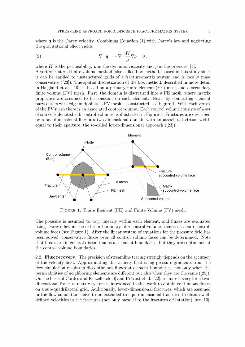
where K is the permeability, µ is the dynamic viscosity and p is the pressure, [4].A vertex-centered finite volume method, also called box method, is used in this study sinceit can be applied to unstructured grids of a fracture-matrix system and is locally massconservative ([23]). The spatial discretization of the box method, described in more detailin Hægland et al. [10], is based on a primary finite element (FE) mesh and a secondaryfinite volume (FV) mesh. First, the domain is discretized into a FE mesh, where matrixproperties are assumed to be constant on each element. Next, by connecting elementbarycenters with edge midpoints, a FV mesh is constructed, see Figure 1. With each vertexof the FV mesh there is an associated control volume. Each control volume consists of a setof sub cells denoted sub control-volumes as illustrated in Figure 1. Fractures are describedby a one-dimensional line in a two-dimensional domain with an associated virtual widthequal to their aperture, the so-called lower-dimensional approach ([23]).

Fracturesubcontrol volume face

Matrixsubcontrol volume face

Fracture

Barycenter

Control volume(Box)

FE mesh

FV mesh

Node

Element

Subcontrol volume

Figure 1. Finite Element (FE) and Finite Volume (FV) mesh.

The pressure is assumed to vary linearly within each element, and fluxes are evaluatedusing Darcy’s law at the exterior boundary of a control volume. denoted as sub control-volume faces (see Figure 1). After the linear system of equations for the pressure field hasbeen solved, conservative fluxes over all control volume faces can be determined. Notethat fluxes are in general discontinuous at element boundaries, but they are continuous atthe control volume boundaries.

2.2. Flux recovery. The precision of streamline tracing strongly depends on the accuracyof the velocity field. Approximating the velocity field using pressure gradients from theflow simulation results in discontinuous fluxes at element boundaries, not only when thepermeabilities of neighboring elements are different but also when they are the same ([25]).On the basis of Cordes and Kinzelbach [6] and Prevost et al. [22], a flux recovery for a two-dimensional fracture-matrix system is introduced in this work to obtain continuous fluxeson a sub-quadrilateral grid. Additionally, lower-dimensional fractures, which are assumedin the flow simulation, have to be extended to equi-dimensional fractures to obtain well-defined velocities in the fractures (not only parallel to the fractures orientation), see [10].


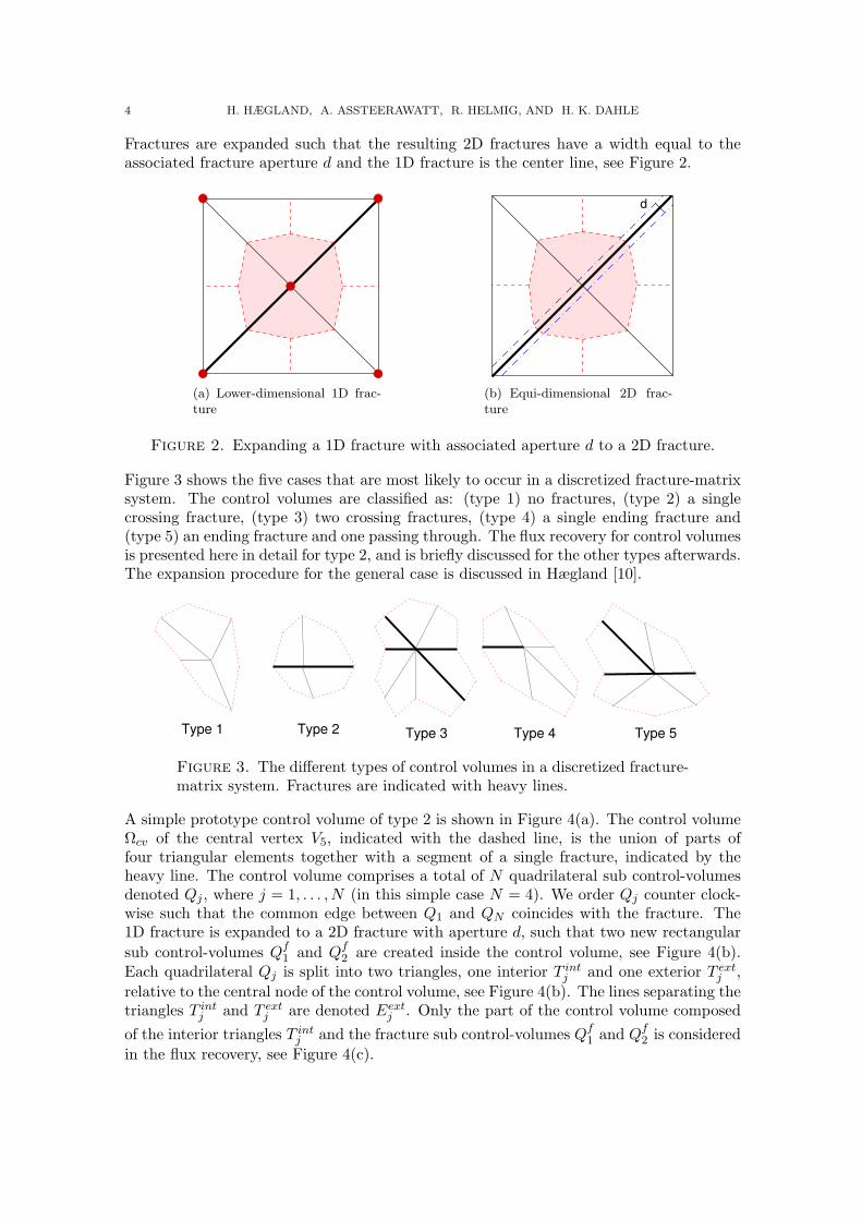
Fractures are expanded such that the resulting 2D fractures have a width equal to theassociated fracture aperture d and the 1D fracture is the center line, see Figure 2.

(a) Lower-dimensional 1D frac-ture

d

(b) Equi-dimensional 2D frac-ture

Figure 2. Expanding a 1D fracture with associated aperture d to a 2D fracture.

Figure 3 shows the five cases that are most likely to occur in a discretized fracture-matrixsystem. The control volumes are classified as: (type 1) no fractures, (type 2) a singlecrossing fracture, (type 3) two crossing fractures, (type 4) a single ending fracture and(type 5) an ending fracture and one passing through. The flux recovery for control volumesis presented here in detail for type 2, and is briefly discussed for the other types afterwards.The expansion procedure for the general case is discussed in Hægland [10].

Type 5Type 3Type 1 Type 2 Type 4

Figure 3. The different types of control volumes in a discretized fracture-matrix system. Fractures are indicated with heavy lines.

A simple prototype control volume of type 2 is shown in Figure 4(a). The control volumeΩcv of the central vertex V5, indicated with the dashed line, is the union of parts offour triangular elements together with a segment of a single fracture, indicated by theheavy line. The control volume comprises a total of N quadrilateral sub control-volumesdenoted Qj , where j = 1, . . . , N (in this simple case N = 4). We order Qj counter clock-wise such that the common edge between Q1 and QN coincides with the fracture. The1D fracture is expanded to a 2D fracture with aperture d, such that two new rectangularsub control-volumes Qf

1 and Qf2 are created inside the control volume, see Figure 4(b).

Each quadrilateral Qj is split into two triangles, one interior T intj and one exterior T ext

j ,relative to the central node of the control volume, see Figure 4(b). The lines separating thetriangles T int

j and T extj are denoted Eext

j . Only the part of the control volume composedof the interior triangles T int

j and the fracture sub control-volumes Qf1 and Qf

2 is consideredin the flux recovery, see Figure 4(c).


V1

V2

V3

V4

V5

C1

C2

C3

C4

Q1Q2

Q3Q4

(a) Four elements (triangles) with ver-tices V1, . . . , V5. A control volume(dashed line) is associated with V5.

C3

C4

C1

C2

T ext3

T ext4

T ext1

T ext2

T int3

T int4

T int1T int

2

Qf2

Qf1

(b) The control volume in the left fig-ure. The fracture has been expandedto a 2D element with aperture d.

Eext3

Eext4

Eext1

Eext2

Eint1

Eint,f2

Eint,f3 Eint

3

Eint,f4

Eint,f1

Ef2

Ef

Ef1

(c) Control-volume edge numbering

n3

n4

n1

n2

νf2,3

ν3,4

νf1,1

ν1,2

(d) Control-volume normal vectors

Figure 4. Flux recovery for a control volume with an internal fracture.

From the flow simulation, fluxes are given over the exterior faces of the control volumeΩcv, as indicated by the dashed line segments in Figure 4(b). The recovery procedurecalculates additional conservative fluxes on the interior matrix edges (Eint

j and Eint,fj )

and the interior fracture edge (Ef ), see Figure 4(c). These fluxes on Eintj and Eint,f

j areobtained indirectly by computing a constant Darcy velocity qj of each interior triangleT int

j .The constant Darcy velocities qj and the fracture interior fluxes F f must satisfy thefollowing conditions

• mass conservation for the exterior triangle T extj :

(3) qj · nj = Fj,1 + Fj,2 , j = 1, . . . , N ,

where nj is the outward normal vector to Eextj relative to T ext

j with its lengthequal to the length of the edge Eext

j , see Figure 4(d). Fluxes Fj,1 and Fj,2 are thegiven fluxes with respect to the outward normal vector of T ext

j at the two edges ofT ext

j which coincides with the ∂Ωcv, see Figure 4(b).


• the flux over the interior boundaries not coinciding with the fracture edges mustbe continuous:

(4) qj · νj,j+1 = qj+1 · νj,j+1 , j = 1, . . . ,M − 1, M + 1, . . . , N − 1 ,

where M is the number of the last interior triangle belonging to Ω1, νj,j+1 is thenormal vector of the interior boundary Eint

j pointing from T intj to T int

j+1 and haslength equal to Eint

j , see Figure 4(d).• mass conservation in one fracture Qf

k is required:

(5) −qj · νfk,j + qj+1 · ν

fk,j + F f + F f

k = 0 ,

where F f is the unknown flux over the fracture interior edge Ef , F fk is the given

flux over the edge of the expanded fracture Qfk , which coincides with a part of

the boundary of the expanded control volume. The sign of the fluxes are chosenaccording to the outward normal vector of Qf

k . Further, νfk,j is a normal vector to

the edge Eint,fj between the fracture k and the interior triangle T int

j and has its

length equal to the edge. The sign of νfk,j is chosen as shown in Figure 4(d). Note

that we consider only one mass conservation for one of the fracture quadrilaterals;mass conservation for the other is automatically fulfilled since the sum of the fluxesout of Ωcv is zero.

A system of 2N − 1 linear equations has now been set up, however, a total number ofunknown components 2N+1 (2N from the qj and 1 from the flux F f ) must be determined.To close the system, we need two more equations, which can be derived by requiring thegradient of the pressure field to be irrotational ([6]). From Equation (2), the Darcy velocityq can be written as

(6) q = −K

µ∇p .

Rearranging Equation (6) and taking the curl of a gradient yield

(7) ∇× µK−1q = −∇×∇p .

Since the curl of a gradient is always zero and the dynamic viscosity µ is constant in thisstudy, we have from Stokes theorem

(8)∫

Ω∇×K−1qdΩ =

∮Γ

K−1q · ds = 0 .

Here, Ω may be any 2D subdomain of the whole solution domain, and Γ is the 1D boundaryof Ω. Equation (8) is now applied over two subdomains, Ω1 and Ω2, separated by thefracture.For this simple case shown in Figure 4(c), the subdomain Ω1 contains T int

1 and T int2 with

its boundary Γ1 corresponding to the counter clockwise sequences of edges Eext1 , Eext

2 ,Eint,f

2 and Eint,f1 . Then, Equation (8) can be written as

(9)∮

Γ1

K−1q · ds =M∑

j=1

∫Eext

j

K−1j qj · ds+

∫Eint,f

2

K−1F qf

2 · ds+∫

Eint,f1

K−1F qf

1 · ds = 0 ,

where the orientation of integration is counter clockwise, M is the number of the lastinterior triangle belonging to Ω1 (here M = 2), and the fracture permeability KF is ascalar.


p21

p22

p23

p24

F f2

F f

Qf2

p11

p12

p13

p14

F f

F f1

Qf1

Figure 5. The four corners points and the direction of fluxes of the frac-ture rectangles.

In the first term of Equation (9), both Kj and qj are constant; hence,

(10)M∑

j=1

∫Eext

j

K−1j qj · ds =

M∑j=1

K−1j qj · tj =

M∑j=1

K−1j tj · qj ,

where the tangent vectors tj corresponds to a 90 degrees counter-clockwise rotation of thenormal vector nj having the length of Eext

j .The second and the third terms in Equation (9) are integrals along the fracture edges.The velocities in the fracture quadrilaterals qf

1 and qf2 are given by linear interpolation of

the edge fluxes using Pollock’s method [20]. This yields

(11)∫

Eint,f2

K−1F qf

2 · ds =(−F f

2 − F f )‖u2‖2KF ‖v2‖

,

and

(12)∫

Eint,f1

K−1F qf

1 · ds =(F f

1 − F f )‖u1‖2KF ‖v1‖

,

where

uk = pk2 − pk

1 and vk = pk4 − pk

1 , k = 1, 2 .(13)

As shown in Figure 5, pki is the coordinate of the corners i of an extended fracture Qf

k

and F fi is the flux over the fracture exterior edge Ef

k given from the flow simulation. Thedetails of the calculation leading to Equations (11) and (12) are presented in the Appendix.

Substituting Equations (10) - (12) in Equation (9) yields

(14)∮

Γ1

K−1q · ds =M∑

j=1

K−1j tj · qj +

(−F f2 − F f )‖u2‖2KF ‖v2‖

+(F f

1 − F f )‖u1‖2KF ‖v1‖

.

A similar argument can be used to show that the line integral along Γ2 can be given as

(15)∮

Γ2

K−1q · ds =N∑

j=M+1

K−1j tj · qj −

(F f1 − F f )‖u1‖2KF ‖v1‖

− (−F f2 − F f )‖u2‖2KF ‖v2‖

.

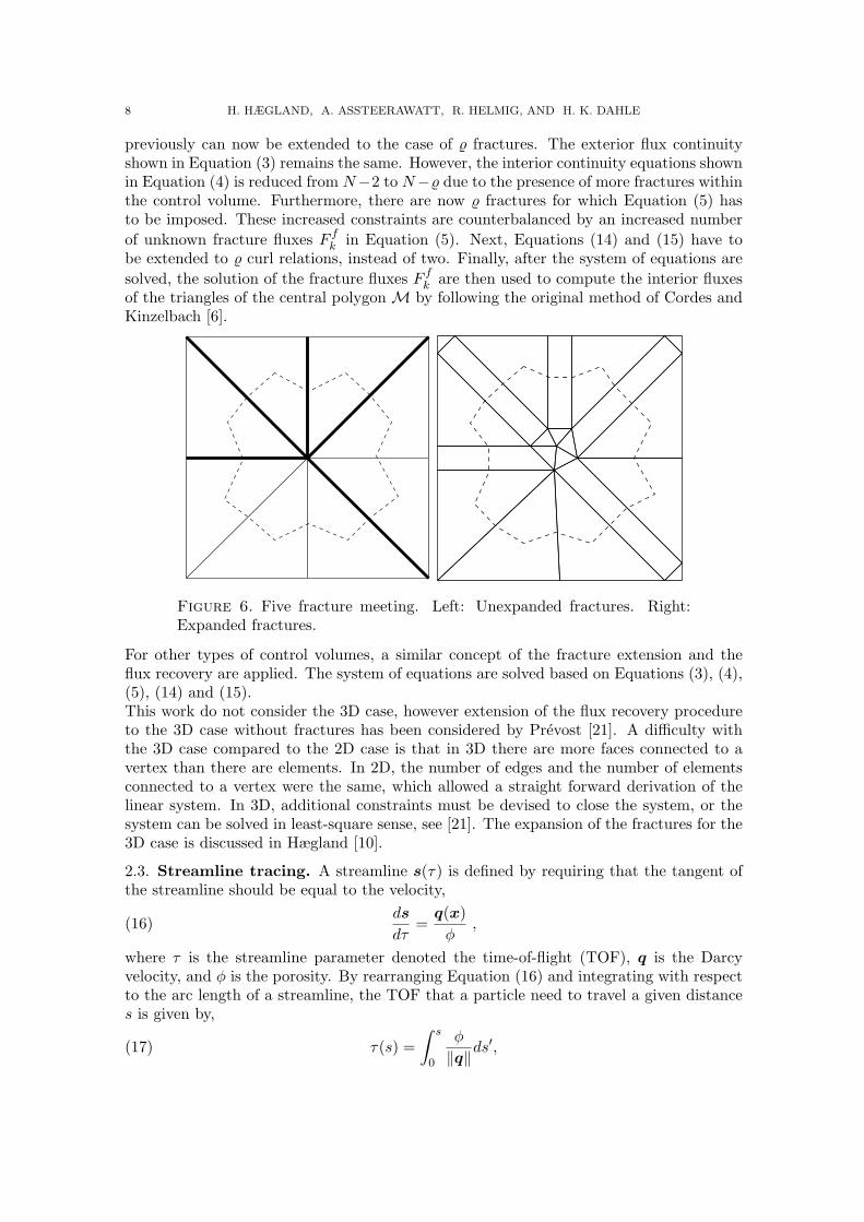
The general case of a discretized fracture-matrix control volume is described by % fracturesmeeting at a vertex (% = 0, 1, 2, ...). A new mesh of expanded fractures is constructed byintroducing a polygon M with % edges at the overlapping area of the % expanded fractures.The % fractures now becomes % trapezoidal elements and the central polygon M is dividedinto % triangles, each having one vertex at the centroid of the polygon. A sketch of a casefor % = 5 is shown in Figure 6. The flux recovery method for two fractures described


previously can now be extended to the case of % fractures. The exterior flux continuityshown in Equation (3) remains the same. However, the interior continuity equations shownin Equation (4) is reduced from N−2 to N−% due to the presence of more fractures withinthe control volume. Furthermore, there are now % fractures for which Equation (5) hasto be imposed. These increased constraints are counterbalanced by an increased numberof unknown fracture fluxes F f

k in Equation (5). Next, Equations (14) and (15) have tobe extended to % curl relations, instead of two. Finally, after the system of equations aresolved, the solution of the fracture fluxes F f

k are then used to compute the interior fluxesof the triangles of the central polygon M by following the original method of Cordes andKinzelbach [6].

Figure 6. Five fracture meeting. Left: Unexpanded fractures. Right:Expanded fractures.

For other types of control volumes, a similar concept of the fracture extension and theflux recovery are applied. The system of equations are solved based on Equations (3), (4),(5), (14) and (15).This work do not consider the 3D case, however extension of the flux recovery procedureto the 3D case without fractures has been considered by Prevost [21]. A difficulty withthe 3D case compared to the 2D case is that in 3D there are more faces connected to avertex than there are elements. In 2D, the number of edges and the number of elementsconnected to a vertex were the same, which allowed a straight forward derivation of thelinear system. In 3D, additional constraints must be devised to close the system, or thesystem can be solved in least-square sense, see [21]. The expansion of the fractures for the3D case is discussed in Hægland [10].

2.3. Streamline tracing. A streamline s(τ) is defined by requiring that the tangent ofthe streamline should be equal to the velocity,

(16)ds

dτ=

q(x)φ

,

where τ is the streamline parameter denoted the time-of-flight (TOF), q is the Darcyvelocity, and φ is the porosity. By rearranging Equation (16) and integrating with respectto the arc length of a streamline, the TOF that a particle need to travel a given distances is given by,

(17) τ(s) =∫ s

0

φ

‖q‖ds′,


where s measures arc length along a streamline. Note that, due to the appearance ofthe porosity in Equation (17), the TOF is related to the particle velocity, not the Darcyvelocity.Methods for streamline tracing on quadrilateral grids when fluxes are known have beeninvestigated by several authors. For a regular quadrilateral mesh (rectangular mesh)Pollock’s method has been widely used. The method assumes a piece-wise linear approx-imation of the velocity over the entire grid. Within a single grid cell taken to be the unitsquare for simplicity, the velocity is given as

(18) q(x) =[

fx0(1− x) + fx1xfy0(1− y) + fy1y

], 0 ≤ x ≤ 1 and 0 ≤ y ≤ 1 ,

where fk are fluxes over the cell faces (see Figure 7). Solving Equation (16) by insertingthe velocity from Equation (18) yields two separate expressions for the TOF:

(19) τx(xi, xj) =φ

fx1 − fx0ln

(fx0 + (fx1 − fx0)xj

fx0 + (fx1 − fx0)xi

),

and

(20) τy(yi, yj) =φ

fy1 − fy0ln

(fy0 + (fy1 − fy0)yj

fy0 + (fy1 − fy0)yi

).

The TOF that a particle travels from the entry point xen to the exit point xex of thegrid cell is determined by calculating the time that a streamline requires to cross the gridboundaries. Inserting xj = 0 and 1 in Equation (19) and yj = 0 and 1 in Equation (20),and replacing xi and yi with xen yield four different times that the streamline requires tocross the left, the right, the bottom and the top boundaries respectively. The TOF is theminimum positive time of the calculated times. By rearranging Equations (19) and (20)and inserting the TOF in τex, the exit point xex is then given as

(21) xex =1

fx1 − fx0

qen,x exp

(τex

φ(fx1 − fx0)

)− fx0

,

(22) yex =1

fy1 − fy0

qen,y exp

(τex

φ(fy1 − fy0)

)− fy0

,

where qen is the velocity at the entry point xen calculated from Equation (18).

fx0 fx1

xex

fy0

xenfy1

y

x0

1

1

v(x)

Figure 7. Pollock tracing for a unit square.


A complex fracture-matrix system can only be discretized precisely with unstructuredgrids. Hence, streamline tracing which performs well on unstructured grids is required.The extension of Pollock’s method on unstructured grids has proven successful in severalstudies [6, 22, 11]. The spatial coordinates together with the velocity in the physical spaceP are transformed to a reference space R by using the bilinear iso-parametric transforma-tion, see Figure 8.

1

2

4

3

y1f

x1f

y0f

x0f

y

x

v

(a) Physical space Py0f’

y1f’

x0f’ x1f’

1 2

34

0 1 x’

y’

1

v’

(b) Reference space R

Figure 8. Transformation of an unstructured grid and edge fluxes from aphysical space P to a reference space R.

According to Hægland et al. [11], the velocity field v′ in R is related to the linear fluxinterpolation as

(23) q′ =dx′

dt=

1det J

[fx0(1− x′i) + fx1x

′i

fy0(1− y′i) + fy1y′i

],

where JJJ is the Jacobian transformation matrix

(24) JJJ =

dx

dx′dx

dy′

dy

dx′dy

dy′

.

The velocity in Equation (23) is rewritten in terms of a pseudo time τ in R as shown byJimenez et al. [13] as

(25) dτ =dt

det J=

dx′

fx0(1− x′i) + fx1x′idy′

fy0(1− y′i) + fy1y′i

,

where t is real time in P. The actual time-of-flight tex is then evaluated by integratingEquation (25) from x′en to x′ex:

(26) tex =∫ t(τex)

0dt =

∫ τex

0det J(x′(τ), y′(τ))dτ .

Recently, some problems with the method have been reported and resolved. Inaccuraciesin computing TOF due to errors in the absolute value of the interpolated velocity fieldhave been reported in [13, 9, 11]. Jimenez et al. [13] proposed an extension of the methodthat allowed for exact reproduction of time-of-flight for uniform flow in 2D. In this paper,we utilize this latter approach, see [9, 11, 13] for more details of the method.


2.4. Evaluation of the breakthrough curve. We assume purely advective transportof a solute tracer in the streamline method and visualize each streamline as a flow channelor a streamtube. Due to the pure advective transport in the streamline method, no massexchanges between neighboring streamtubes. The TOF measures the time that the tracerneeds to travel along the streamtube, see Figure 9. Streamlines are distributed equallyaccording to the total flux along the inflow boundary, such that each streamtube containsthe same flux.

streamline

streamtube

block mass

(related to injection period dt)dx

Figure 9. Mass transport in a streamtube as a block.

The transport behavior characterized from the results of the streamline method are de-scribed using a breakthrough curve (BTC) and an accumulated breakthrough curve (Ac-cBTC). The latter is the sum of the total mass leaving the domain at the outflow boundaryuntil a time t and BTC is the rate of change of AccBTC during the time interval ∆t

BTC(t) =AccBTC(t)−AccBTC(t−∆t)

∆t,(27)

AccBTC(t) = AccBTC(t−∆t) + msn∑

i=1

Ti ,(28)

where ms is the normalized mass flux, which is determined by the mass flux in eachstreamtube over the total injected mass, and n is the total number of the streamtubes.The arrival time condition Ti, for a streamtube i, is given as

(29) Ti(t) =

0 ; t < TOFi

t− TOFi ; TOFi ≤ t ≤ TOFi + dt0 ; t > TOFi + dt

where the time of flight TOFi is the time that a block mass in a streamtube i travels untilit reaches the outflow boundary and dt is the duration of mass injection.The TOF of each streamtube is a discrete value, which can be the same for all streamtubesor highly varied depending on the geometries and structures of a domain. The overalltransport behavior of the system is presented as a histogram BTC which evaluates therate of change of the normalized mass flux over a specified interval of time.

3. Comparison Results

3.1. Preliminary test case. In order to understand the difference arising from simulat-ing the transport process using grid-based advective transport (ADT) and the streamlinemethod (STR), three preliminary test cases are set up: a single short fracture, a singlelong fracture and systematically distributed fractures, see Figure 10 (top). For all testcases, a two-dimensional domain of 1.0 × 1.0 m is set up. The fluid properties and thedomain properties correspond to the data presented in Table 1.


We consider transport of a solute tracer without dispersion and the governing equationcan be written as

(30)∂c

∂t+∇ · q

φc = 0 .

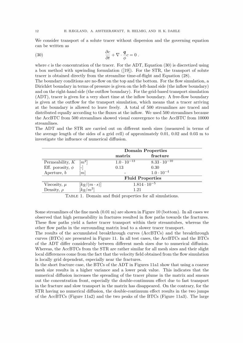
where c is the concentration of the tracer. For the ADT, Equation (30) is discretized usinga box method with upwinding formulation ([19]). For the STR, the transport of solutetracer is obtained directly from the streamline time-of-flight and Equation (28).The boundary conditions are no-flow on the top and the bottom. For the flow simulation, aDirichlet boundary in terms of pressure is given on the left-hand side (the inflow boundary)and on the right-hand side (the outflow boundary). For the grid-based transport simulation(ADT), tracer is given for a very short time at the inflow boundary. A free-flow boundaryis given at the outflow for the transport simulation, which means that a tracer arrivingat the boundary is allowed to leave freely. A total of 500 streamlines are traced anddistributed equally according to the fluxes at the inflow. We used 500 streamlines becausethe AccBTC from 500 streamlines showed visual convergence to the AccBTC from 10000streamlines.The ADT and the STR are carried out on different mesh sizes (measured in terms ofthe average length of the sides of a grid cell) of approximately 0.01, 0.02 and 0.03 m toinvestigate the influence of numerical diffusion.

Domain Propertiesmatrix fracture

Permeability, K [m2] 1.0 · 10−13 8.33 · 10−10

Eff. porosity, φ [-] 0.13 0.30Aperture, b [m] - 1.0 · 10−4

Fluid PropertiesViscosity, µ [kg/(m · s)] 1.814 · 10−5

Density, ρ [kg/m3] 1.21Table 1. Domain and fluid properties for all simulations.

Some streamlines of the fine mesh (0.01 m) are shown in Figure 10 (bottom). In all cases weobserved that high permeability in fractures resulted in flow paths towards the fractures.These flow paths yield a faster tracer transport within their streamtubes, whereas theother flow paths in the surrounding matrix lead to a slower tracer transport.The results of the accumulated breakthrough curves (AccBTCs) and the breakthroughcurves (BTCs) are presented in Figure 11. In all test cases, the AccBTCs and the BTCsof the ADT differ considerably between different mesh sizes due to numerical diffusion.Whereas, the AccBTCs from the STR are rather similar for all mesh sizes and their slightlocal differences come from the fact that the velocity field obtained from the flow simulationis locally grid dependent, especially near the fractures.In the short fracture case, the BTCs of the ADT in Figures 11a1 show that using a coarsermesh size results in a higher variance and a lower peak value. This indicates that thenumerical diffusion increases the spreading of the tracer plume in the matrix and smearsout the concentration front, especially the double-continuum effect due to fast transportin the fracture and slow transport in the matrix has disappeared. On the contrary, for theSTR having no numerical diffusion, the double-continuum effect results in the two jumpsof the AccBTCs (Figure 11a2) and the two peaks of the BTCs (Figure 11a3). The large


X

Y

0 0.2 0.4 0.6 0.8 10

0.2

0.4

0.6

0.8

1

X

Y

0 0.2 0.4 0.6 0.8 10

0.2

0.4

0.6

0.8

1

X

Y

0 0.2 0.4 0.6 0.8 10

0.2

0.4

0.6

0.8

1

Figure 10. Top: Domains with fractures. Middle: Discretization domains(top) for a mesh size of 0.01 m corresponding to ca. 11700 vertices. Bottom:25 of the 500 streamlines traced for the grids in the middle row.

part of the tracer transported in the matrix arrives about the same time at the outflowand results in a very high mass flux in the second peak of the BTC and a sharp rise of thesecond jump in the AccBTC.When the fracture becomes longer (Figure 11b), the double-continuum effect can also benoticed for the ADT, in spite of the numerical diffusion, see Figures 11b1 and 11b2. Thefast transport in the long fracture results in the first peak of the BTCs; later, the partof the tracer plume transported in the matrix leads to the second peak. The numericaldiffusion in the transversal flow-direction causes spreading of mass transported in thefracture to the surrounding matrix. Therefore, the value of the first peak of the BTCof the STR is higher than that of the ADT (see Figure 11b3) and the AccBTCs show asharp rise for the STR, but only a gradual increase for the ADT (see Figures 11b2). Thiseffect delays the arrival time of the mass transported in the fracture. The influence of thenumerical diffusion on the part of the tracer transported through the porous matrix showsthe same behavior as that observed in the BTCs for the single short fracture, as discussedabove.


(a1) (b1) (c1)

(a2) (b2) (c2)

(a3) (b3) (c3)

Figure 11. Transport simulation results of ADT and STR for the testcases: a) (left column) a single short fracture, b) (middle column) a singlelong fracture and c) (right column) systematically distributed fractures.Top row (a1/b1/c1): BTC of ADT for different mesh sizes. Middle row(a2/b2/c2): AccBTC of ADT and STR for different mesh sizes. Bottomrow (a3/b3/c3): BTC of ADT and STR at a mesh size of 0.01 m.

Increasing the number of horizontal fractures with a vertical fracture connecting all hori-zontal fractures (Figure 11c) increases the part of tracer transported in the fractures anddecreases the part transported in the matrix. Therefore, the BTCs in Figure 11c1 show ahigh peak and the AccBTCs in Figure 11c2 show a high first jump. Due to the influence ofthe numerical diffusion in the ADT, the BTCs of the coarse mesh size of 0.03 and 0.02 mshow only a long tail, whereas the BTC of the fine mesh size of 0.01 m has a small secondpeak (see Figure 11c1), more similar to the BTC of the STR showing a double-continuumeffect as can be seen in Figure 11c3. The effect of the numerical diffusion along fracturesin the transversal flow-direction can be better noticed in this case than in the single longfracture case. As the mesh gets finer and the numerical diffusion decreases, the tracertransported in the fractures remains more confined to the fractures and arrives faster atthe outflow and this yields a BTC with a slightly higher peak concentration shifted some-what to the left compared to the BTCs of the coarser mesh sizes (see Figure 11c1). TheAccBTCs of the ADT seem to converge to the result of the STR when the mesh becomesfiner and the numerical diffusion decreases, see Figure 11c2.


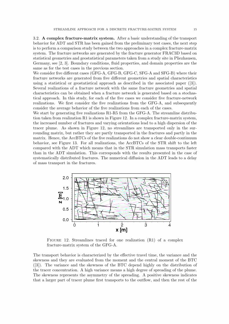
3.2. A complex fracture-matrix system. After a basic understanding of the transportbehavior for ADT and STR has been gained from the preliminary test cases, the next stepis to perform a comparison study between the two approaches in a complex fracture-matrixsystem. The fracture networks are generated by the fracture generator FRAC3D based onstatistical geometries and geostatistical parameters taken from a study site in Pliezhausen,Germany, see [2, 3]. Boundary conditions, fluid properties, and domain properties are thesame as for the test cases in the previous section.We consider five different cases (GFG-A, GFG-B, GFG-C, SFG-A and SFG-B) where theirfracture networks are generated from five different geometries and spatial characteristicsusing a statistical or geostatistical approach as described in the associated paper ([3]).Several realizations of a fracture network with the same fracture geometries and spatialcharacteristics can be obtained when a fracture network is generated based on a stochas-tical approach. In this study, for each of the five cases we consider five fracture-networkrealizations. We first consider the five realizations from the GFG-A, and subsequentlyconsider the average behavior of the five realizations from each of the cases.We start by generating five realizations R1-R5 from the GFG-A. The streamline distribu-tion taken from realization R1 is shown in Figure 12. In a complex fracture-matrix system,the increased number of fractures and varying orientations lead to a high dispersion of thetracer plume. As shown in Figure 12, no streamlines are transported only in the sur-rounding matrix, but rather they are partly transported in the fractures and partly in thematrix. Hence, the AccBTCs of the five realizations do not show a clear double-continuumbehavior, see Figure 13. For all realizations, the AccBTCs of the STR shift to the leftcompared with the ADT which means that in the STR simulation mass transports fasterthan in the ADT simulation. This corresponds with the results presented in the case ofsystematically distributed fractures. The numerical diffusion in the ADT leads to a delayof mass transport in the fractures.

Figure 12. Streamlines traced for one realization (R1) of a complexfracture-matrix system of the GFG-A.

The transport behavior is characterized by the effective travel time, the variance and theskewness and they are evaluated from the moment and the central moment of the BTC([3]). The variance and the skewness of the BTC depend highly on the distribution ofthe tracer concentration. A high variance means a high degree of spreading of the plume.The skewness represents the asymmetry of the spreading. A positive skewness indicatesthat a larger part of tracer plume first transports to the outflow, and then the rest of the


ADTSTR

0

0.2

0.4

0.6

0.8

1

0 80000 160000 240000

Acc.

rati

o m

ass

[−

]

Time [s]

(a) R1

ADTSTR

0

0.2

0.4

0.6

0.8

1

0 80000 160000 240000

Acc.

rati

o m

ass

[−

]

Time [s]

(b) R2

ADTSTR

1

0

0.2

0.4

0.6

0.8

0 80000 160000 240000

Acc.

rati

o m

ass

[−

]

Time [s]

(c) R3

ADTSTR

0

0.2

0.4

0.6

0.8

1

0 80000 160000

Acc.

rati

o m

ass

[−

]

Time [s]

240000

(d) R4

ADTSTR

0

0.2

0.4

0.6

0.8

1

0 80000 160000 240000

Acc.

rati

o m

ass

[−

]

Time [s]

(e) R5

Figure 13. AccBTCs of ADT and STR for the complex fracture-matrixsystems for five realizations (R1-R5) of the GFG-A.

plume arrives gradually. The faster mass transport in the STR leads to a less effectivetravel time compared with the transport in the ADT (see Figure 14a). For all realizations,higher variances and higher skewnesses are seen in the STR compared to the ADT (seeFigures 14b and 14c). This is due to the fact that the fast transport in the fractures andthe slow transport in the matrix are better captured with the STR, whereas the numericaldiffusion in the ADT smears out this contrast.

ADTSTR

5.0e+04

5.5e+04

6.0e+04

6.5e+04

7.0e+04

7.5e+04

8.0e+04

R1 R2 R3 R4 R5

Eff

ecti

ve t

ravel

tim

e [

s]

(a) Effective travel time.

ADTSTR

3.0e+08

4.0e+08

5.0e+08

6.0e+08

7.0e+08

8.0e+08

9.0e+08

1.0e+09

1.1e+09

1.2e+09

R1 R2 R3 R4 R5

Vari

ance [

s ]

2

(b) Variance.

ADTSTR

2.0e−01

4.0e−01

6.0e−01

8.0e−01

1.0e+00

1.2e+00

1.4e+00

1.6e+00

1.8e+00

2.0e+00

R1 R2 R3 R4 R5

Ske

wne

ss [−

]

(c) Skewness.

Figure 14. Quantitative results of ADT and STR for the complexfracture-matrix systems of five realizations from the GFG-A.

In the last part of this section we consider the average behavior for the five cases GFG-A, GFG-B, GFG-C, SFG-A and SFG-B. The details about the fracture generation arepresented in the associated paper ([3]). For each case, five realizations are generated andthe results presented for each case are the average values over all five realizations.


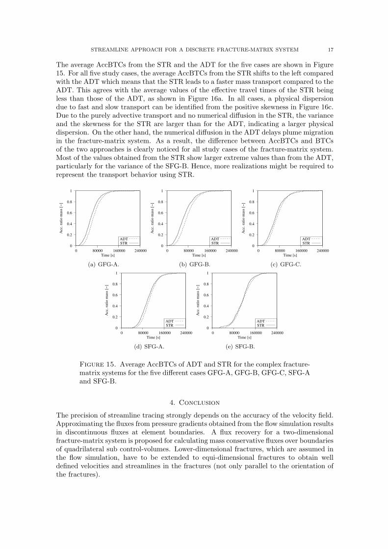
The average AccBTCs from the STR and the ADT for the five cases are shown in Figure15. For all five study cases, the average AccBTCs from the STR shifts to the left comparedwith the ADT which means that the STR leads to a faster mass transport compared to theADT. This agrees with the average values of the effective travel times of the STR beingless than those of the ADT, as shown in Figure 16a. In all cases, a physical dispersiondue to fast and slow transport can be identified from the positive skewness in Figure 16c.Due to the purely advective transport and no numerical diffusion in the STR, the varianceand the skewness for the STR are larger than for the ADT, indicating a larger physicaldispersion. On the other hand, the numerical diffusion in the ADT delays plume migrationin the fracture-matrix system. As a result, the difference between AccBTCs and BTCsof the two approaches is clearly noticed for all study cases of the fracture-matrix system.Most of the values obtained from the STR show larger extreme values than from the ADT,particularly for the variance of the SFG-B. Hence, more realizations might be required torepresent the transport behavior using STR.

ADTSTR

0

0.2

0.4

0.6

0.8

1

0 80000 160000 240000

Acc.

rati

o m

ass

[−

]

Time [s]

(a) GFG-A.

ADTSTR

0

0.2

0.4

0.6

0.8

1

0 80000 160000 240000

Acc.

rati

o m

ass

[−

]

Time [s]

(b) GFG-B.

ADTSTR

0

0.2

0.4

0.6

0.8

1

0 80000 160000 240000

Acc.

rati

o m

ass

[−

]

Time [s]

(c) GFG-C.

ADTSTR

0

0.2

0.4

0.6

0.8

1

0 80000 160000 240000

Acc.

rati

o m

ass

[−

]

Time [s]

(d) SFG-A.

ADTSTR

0

0.2

0.4

0.6

0.8

1

0 80000 160000 240000

Acc.

rati

o m

ass

[−

]

Time [s]

(e) SFG-B.

Figure 15. Average AccBTCs of ADT and STR for the complex fracture-matrix systems for the five different cases GFG-A, GFG-B, GFG-C, SFG-Aand SFG-B.

4. Conclusion

The precision of streamline tracing strongly depends on the accuracy of the velocity field.Approximating the fluxes from pressure gradients obtained from the flow simulation resultsin discontinuous fluxes at element boundaries. A flux recovery for a two-dimensionalfracture-matrix system is proposed for calculating mass conservative fluxes over boundariesof quadrilateral sub control-volumes. Lower-dimensional fractures, which are assumed inthe flow simulation, have to be extended to equi-dimensional fractures to obtain welldefined velocities and streamlines in the fractures (not only parallel to the orientation ofthe fractures).


5.0e+04

6.0e+04

7.0e+04

8.0e+04

9.0e+04

1.0e+05

1.1e+05

1.2e+05

1.3e+05

SFG−ASFG−BGFG−AGFG−BGFG−C

Effe

ctiv

e A

rriv

al T

ime

[s]

STRADT

(a) Effective travel time.

4.0e+08

6.0e+08

8.0e+08

1.0e+09

1.2e+09

1.4e+09


Var

ianc

e [s

]

STRADT

(b) Variance.

−5.0e−01

0.0e+00

5.0e−01

1.0e+00

1.5e+00

2.0e+00


Ske

wne

ss [−

]

STRADT

(c) Skewness.

Figure 16. Average and extreme values (min./max.) obtained from theADT and the STR for the complex fracture-matrix systems for the fivedifferent cases.

The applicability of a streamline method (STR) for the study of the transport behavior ina fracture-matrix system is investigated by comparing with the results from a grid-basedadvective transport (ADT) model. In the simple cases of one fracture or systematicallydistributed fractures, the effect of fast flow in the fractures and slow flow in the matrixis smeared out due to the numerical diffusion in the ADT. The preferential flow paths inthe fracture-matrix system are clearly noticed in the STR from the double-peak BTCsand two sudden rises in the AccBTCs. In the complex fracture-matrix system consistingof a large number of fractures with varying orientations, numerical diffusion in the ADTdelays plume migration, whereas purely advective transport in the STR leads to fastsolute transport and maintains a high physical dispersion due to the fast transport in thefractures and slow transport in the matrix. As a result, we observe a less effective traveltime, higher variance and higher skewness from the STR than from the ADT as well as ashift of AccBTC of the STR to the left.Further investigations involving comparisons with experimental or field studies have to becarried out in order to validate the results of the STR. If the assumption of the purelyadvective transport in the STR leads to an acceleration of the tracer transport in thesystem compared with the measurement results, including dispersive transport in theSTR could be considered to improve the STR approach.

5. Appendix

The integral of the velocity along the fracture edge is computed by assuming that thevelocities in the quadrilateral fracture are given by linear interpolation of the edge fluxessimilar to Pollock’s method ([20]). Following Prevost et al. [22] and Jimenez et al. [13],the rectangle Qf

1 (see Figure 4(b)) in P is transformed to a unit square in a referencespace R using the bilinear transformation x(x, y), which simplifies for a rectangle (Figure17 (right)) to,

(31) p(x, y) = p1 + (p2 − p1)x + (p4 − p1)y ,

with the constant Jacobian matrix,

(32) J =[x2 − x1 x4 − x1

y2 − y1 y4 − y1

]=

[u v

],

where u and v are the shape vectors of the rectangle, and xi is the point at corner i

see Figure 17 (left). Edge fluxes Fx0, Fx1, Fy0, and Fy1, are defined for Qf1 with positive


v

u

p1

p2

p3

p4Fx0

Fx1

Fy0

Fy1

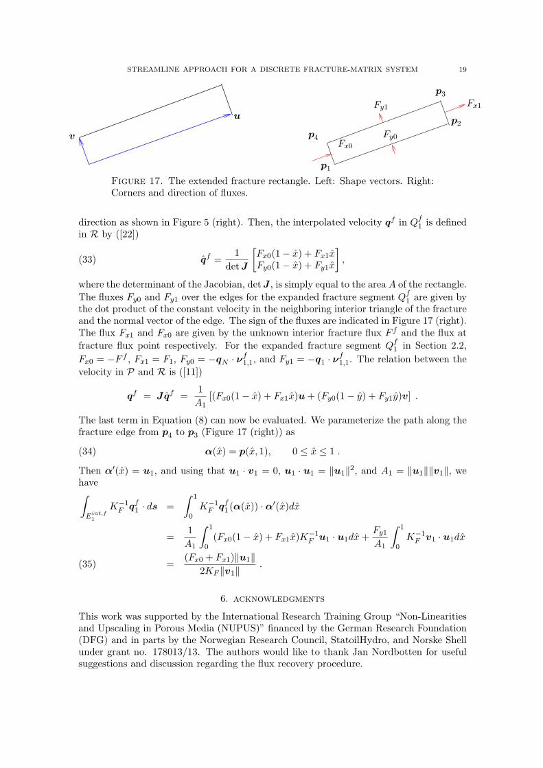
Figure 17. The extended fracture rectangle. Left: Shape vectors. Right:Corners and direction of fluxes.

direction as shown in Figure 5 (right). Then, the interpolated velocity qf in Qf1 is defined

in R by ([22])

(33) qf =1

det J

[Fx0(1− x) + Fx1xFy0(1− x) + Fy1x

],

where the determinant of the Jacobian, detJ , is simply equal to the area A of the rectangle.The fluxes Fy0 and Fy1 over the edges for the expanded fracture segment Qf

1 are given bythe dot product of the constant velocity in the neighboring interior triangle of the fractureand the normal vector of the edge. The sign of the fluxes are indicated in Figure 17 (right).The flux Fx1 and Fx0 are given by the unknown interior fracture flux F f and the flux atfracture flux point respectively. For the expanded fracture segment Qf

1 in Section 2.2,Fx0 = −F f , Fx1 = F1, Fy0 = −qN · νf

1,1, and Fy1 = −q1 · νf1,1. The relation between the

velocity in P and R is ([11])

qf = Jqf =1

A1[(Fx0(1− x) + Fx1x)u + (Fy0(1− y) + Fy1y)v] .

The last term in Equation (8) can now be evaluated. We parameterize the path along thefracture edge from p4 to p3 (Figure 17 (right)) as

(34) α(x) = p(x, 1), 0 ≤ x ≤ 1 .

Then α′(x) = u1, and using that u1 · v1 = 0, u1 · u1 = ‖u1‖2, and A1 = ‖u1‖‖v1‖, wehave∫

Eint,f1

K−1F qf

1 · ds =∫ 1

0K−1

F qf1(α(x)) ·α′(x)dx

=1

A1

∫ 1

0(Fx0(1− x) + Fx1x)K−1

F u1 · u1dx +Fy1

A1

∫ 1

0K−1

F v1 · u1dx

=(Fx0 + Fx1)‖u1‖

2KF ‖v1‖.(35)

6. acknowledgments

This work was supported by the International Research Training Group “Non-Linearitiesand Upscaling in Porous Media (NUPUS)” financed by the German Research Foundation(DFG) and in parts by the Norwegian Research Council, StatoilHydro, and Norske Shellunder grant no. 178013/13. The authors would like to thank Jan Nordbotten for usefulsuggestions and discussion regarding the flux recovery procedure.


References

[1] Al-Huthali, A., and A. Datta-Gupta, Streamline simulation of counter-current imbibition in naturallyfractured reservoir, J. Petrol. Sci. Eng., 43(3-4), 271-300, 2004.

[2] Assteerawatt, A., Flow and Transport Modelling of Fractured Aquifers based on a Geostatistical Ap-proach, (http://elib.uni-stuttgart.de/opus/volltexte/2008/3639/), PhD Thesis, Universitat Stuttgart,Institute of Hydraulic Engineering, 2008.

[3] Assteerawatt, A., H. Hægland, R. Helmig, A. Bardossy and H. K. Dahle, Simulation of flow andtransport processes in a discrete fracture-matrix system I. geostatistical generation of fractures on anaquifer analogue scale, Water Resour. Res., submitted.

[4] Bear, J., Dynamics of Fluids in Porous Media, Academic Press, California, 1972.[5] Cockburn, B., J. Gopalakrishnan, and H. Wang, Locally conservative fluxes for the continuous

Galerkin method, SIAM J. Numer. Anal., 45(4), 1742-1776, 2007.[6] Cordes, C., and W. Kinzelbach, Continuous groundwater velocity fields and path lines in linear,

bilinear, and trilinear finite elements, Water Resour. Res., 28(11), 2903-2911, 1992.[7] Correa, M.R., and A.F.D. Loula., Stabilized velocity post-processing for Darcy flow in heterogeneous

porous media, Commun. Numer. Meth. En., 23, 461-489, 2007.[8] Durlofsky, L.J., Accuracy of mixed and control volume finite element approximations to Darcy velocity

and related quantities, Water Resour. Res., 30(4), 965-973, 1994.[9] Hægland, H., Streamline tracing on irregular grids (http://www.mi.uib.no/˜hakonh/thesis/thesis.pdf),

Master’s thesis, University of Bergen, Dept. of Mathematics, 2003.[10] Hægland, H., A. Assteerawatt, H. Dahle, G.T. Eigestad, and R. Helmig, Comparison of cell- and

vertex centered discretization methods for flow in a discrete fracture-matrix system, in preparation.[11] Hægland, H., H.K. Dahle, G.T. Eigestad, K.-A. Lie, and I. Aavatsmark, Improved streamlines and

time-of-flight for streamline simulation on irregular grids, Adv. Water Resour., 30(4), 1027-1045, 2007.[12] Huang, W., G.D. Donato, and M.J. Blunt, Comparison of streamline-based and grid-based dual

porosity simulation, J. Petrol. Sci. Eng., 43(1-2), 129-137, 2004.[13] Jimenez, E., K. Sabir, A. Datta-Gupta, and M.J. King, Spatial error and convergence in streamline

simulation, SPE Reserv. Eval. Eng., 10(3), 221-232, June 2007.[14] Karimi-Fard, M., L.J. Durlofsky, and K. Aziz, An efficient discrete fracture model applicable for

general purpose reservoir simulators, SPE J., 227-236, June 2004.[15] King, M.J., and A. Datta-Gupta, Streamline simulation: A current perspective, In Situ, 22(1), 91-140,

1998.[16] Lee, S.H., M.F. Lough, and C.L. Jensen Hierarchical modeling of flow in naturally fractured formations

with multiple length scales, Water Resour. Res., 37(3), 443-455, 2001.[17] Ma, J., G.D. Couples, and S.D. Harris, A mixed finite element technique based on implicit discretiza-

tion of faults for permeability upscaling in fault damage zones, Water Resour. Res., 42, W08413,doi:10.1029/2005WR004686, 2006.

[18] Matringe, S.F., R. Juanes and H.A. Tchelepi, Robust streamline tracing for the simulationof porous media flow on general triangular and quadrilateral grids, J. Comput. Phys., 219(2),doi:10.1016/j.jcp.2006.07.004, 2006.

[19] Neunhauserer, L., Diskretisierungsansatze zur Modellierung von Stromungs- und Transportprozessenin gekluftet-porosen Medien (http://elib.uni-stuttgart.de/opus/volltexte/2003/1477/), PhD Thesis,Universitat Stuttgart, Institute of Hydraulic Engineering, 2003.

[20] Pollock, D.W., Semi-analytical computation of path lines for finite-difference models, Ground Water,26(6), 743-750, 1988.

[21] Prevost, M. Accurate coarse reservoir modeling using unstructured grids, flow-based upscaling andstreamline simulation (http://geothermal.standford.edu/pereposts/search.htm), PhD Thesis, Univer-sity of Standford, 2003.

[22] Prevost, M., M.G. Edwards, and M.J. Blunt, Streamline tracing on curvilinear structured and un-structured grids, SPE J., 139-148, June 2002.

[23] Reichenberger, V., H. Jakobs, P. Bastian, and R. Helmig, A mixed-dimensional finite volume methodfor two-phase flow in fractured porous media, Adv. Water Resour., 29(7), 1020-1036, 2006.

[24] Silberhorn-Hemminger, A., Modellierung von Kluftaquifersystemen: Geostatistis-che analyse und deterministisch – stochastische Kluftgenerierung (http://elib.uni-stuttgart.de/opus/volltexte/2003/1278/), PhD Thesis, Universitat Stuttgart, Institute of HydraulicEngineering, 2002.


[25] Srivastava, R., and M.L. Brusseau, Darcy velocity computations in the finite element method formultidimensional randomly heterogeneous porous media, Adv. Water Resour., 18(4), 191-201, 1995.

[26] Sun, S., and M.F. Wheeler, Projections of velocity data for the compatibility with transport, Comput.Methods Appl. Mech. Engrg., 195, 653-673, 2006.

[27] Thiele, M.R., Streamline simulation, In Proceedings of the 8th International Forum on ReservoirSimulation, Stresa / Lago Maggiore, Italy, 2005.

Documents

SIMULATION OF FLOW AND TRANSPORT PROCESSES IN A DISCRETE …