SIMULATION OF FAILURE IN GEARBOX USING MSC · PDF fileSIMULATION OF FAILURE IN GEARBOX USING MSC.ADAMS ... Keywords: gearbox, cracked tooth, simulation, model, vibration signal, contact

419

ACTA UNIVERSITATIS AGRICULTURAE ET SILVICULTURAE MENDELIANAE BRUNENSIS

Volume 65 45 Number 2, 2017

https://doi.org/10.11118/actaun201765020419

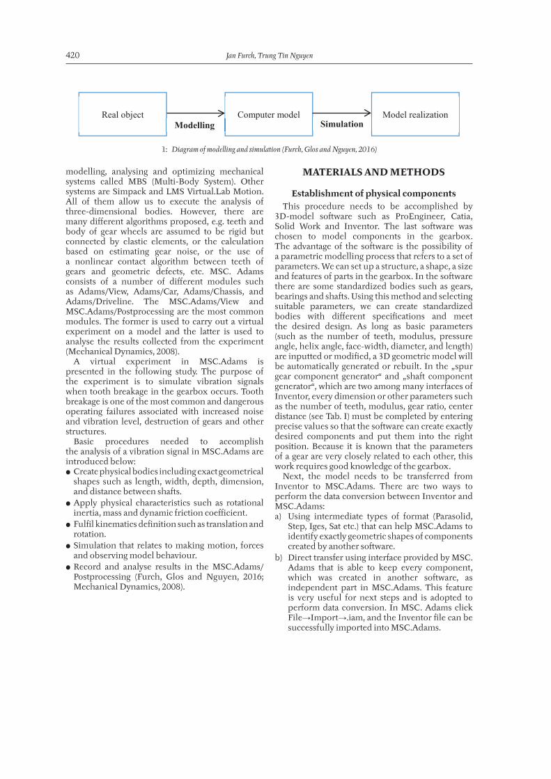
SIMULATION OF FAILURE IN GEARBOX USING MSC.ADAMS

Jan Furch1, Trung Tin Nguyen1

1 Department of Combat and Special Vehicles, Faculty of Military Technology, University of Defence, Kounicova 65, 662 10 Brno, Czech Republic

Abstract

FURCH JAN, TIN NGUYEN TRUNG. 2017. Simulation of Failure in Gearbox Using MSC.Adams. Acta Universitatis Agriculturae et Silviculturae Mendelianae Brunensis, 65(2): 419–428.

Vehicle’s gearbox is regarded as one of the most crucial elements in a vehicle but it sustains a variety of faults such as a broken tooth, misalignment, imbalance, looseness, and even a broken case. Using accelerometers, which are mounted on the case to measure a vibration signal, we can detect faults and monitor the condition but the signals are often complicated and difficult to interpret. Moreover, it is costly and almost impossible to change the structure of a gearbox in order to survey, for instance, the dependence of a vibration signal on the structure, or types of a fault. In this paper a dynamic model of gearbox was developed with tooth breakage to study the capability of simulation using MSC.Adams software. In this simulation we focus on the gearbox used in a common military vehicle. The simulation was based on a nonlinear contact force to predict what happens to the gearbox in case the tooth breaks. The contact mechanics model of the meshing teeth is studied thoroughly by selecting contact simulation parameters such as stiffness, force exponent, damping and friction coefficients. To simulate the real working environment of the gearbox, simulated bearings were also built in the MSC.Adams. The paper shows that it is possible to simulate vibration signals by the gearbox model created in 3D CAD software and analyze the results in the multi‑body dynamics software MSC.Adams.

Keywords: gearbox, cracked tooth, simulation, model, vibration signal, contact force, MSC.Adams.

INTRODUCTIONIn practice the aim of modelling is to understand

the physical phenomena, imitate the behaviour of the examined machine in virtual environments, simulate it on a model and then affect its behaviour by a specific way. The virtual model is just an approximation of reality since the real system can be very complex and the model might not fit the system completely.

Modelling and simulation are two slightly different processes but usually carried out together. They are used to make models based on a real object and allow us to experiment with these models (see Fig. 1).

In the paper by Novotny, Prokop, Zubik and Rehak, 2016, there are introduced advanced computational models suitable for developing a modern powertrain and focusing on noise and vibration. The aim is to decide to what extent the model should be accurate in order to describe

correctly the vibrational and acoustic performance of the powertrain.

The modelling of the dynamics is really useful in case of conditional monitoring, since it allows us to simulate a vibration signal for different conditions of a gearbox which sometimes cannot be checked in an experimental way. There are several methods to simulate the behaviour of a gearbox such as mathematic modelling (e.g. Matlab Simulink), finite element methods (e.g. Ansys) and multi‑body dynamic methods (e.g. MSC.Adams). The last approach seems to be the most suitable for a vibration signal analysis, because it allows us to analyse contact force in the time domain even in the spectrum which has the ability to express exactly the nonlinear effects of stiffness, gear backlash, rotation bearings, eccentricity, misalignment, unbalance and other nonlinear phenomena.

MSC.Adams (Automatic Dynamic Analysis of Mechanical System) is computing software used for

420 Jan Furch, Trung Tin Nguyen

modelling, analysing and optimizing mechanical systems called MBS (Multi‑Body System). Other systems are Simpack and LMS Virtual.Lab Motion. All of them allow us to execute the analysis of three‑dimensional bodies. However, there are many diff erent algorithms proposed, e.g. teeth and body of gear wheels are assumed to be rigid but connected by elastic elements, or the calculation based on estimating gear noise, or the use of a nonlinear contact algorithm between teeth of gears and geometric defects, etc. MSC. Adams consists of a number of diff erent modules such as Adams/View, Adams/Car, Adams/Chassis, and Adams/Driveline. The MSC.Adams/View and MSC.Adams/Postprocessing are the most common modules. The former is used to carry out a virtual experiment on a model and the latter is used to analyse the results collected from the experiment (Mechanical Dynamics, 2008).

A virtual experiment in MSC.Adams is presented in the following study. The purpose of the experiment is to simulate vibration signals when tooth breakage in the gearbox occurs. Tooth breakage is one of the most common and dangerous operating failures associated with increased noise and vibration level, destruction of gears and other structures.

Basic procedures needed to accomplish the analysis of a vibration signal in MSC.Adams are introduced below: • Create physical bodies including exact geometrical

shapes such as length, width, depth, dimension, and distance between shaft s.

• Apply physical characteristics such as rotational inertia, mass and dynamic friction coeffi cient.

• Fulfi l kinematics defi nition such as translation and rotation.

• Simulation that relates to making motion, forces and observing model behaviour.

• Record and analyse results in the MSC.Adams/Postprocessing (Furch, Glos and Nguyen, 2016; Mechanical Dynamics, 2008).

MATERIALS AND METHODS

Establishment of physical componentsThis procedure needs to be accomplished by

3D‑model soft ware such as ProEngineer, Catia, Solid Work and Inventor. The last soft ware was chosen to model components in the gearbox. The advantage of the soft ware is the possibility of a parametric modelling process that refers to a set of parameters. We can set up a structure, a shape, a size and features of parts in the gearbox. In the soft ware there are some standardized bodies such as gears, bearings and shaft s. Using this method and selecting suitable parameters, we can create standardized bodies with diff erent specifi cations and meet the desired design. As long as basic parameters (such as the number of teeth, modulus, pressure angle, helix angle, face‑width, diameter, and length) are inputted or modifi ed, a 3D geometric model will be automatically generated or rebuilt. In the „spur gear component generator“ and „shaft component generator“, which are two among many interfaces of Inventor, every dimension or other parameters such as the number of teeth, modulus, gear ratio, center distance (see Tab. I) must be completed by entering precise values so that the soft ware can create exactly desired components and put them into the right position. Because it is known that the parameters of a gear are very closely related to each other, this work requires good knowledge of the gearbox.

Next, the model needs to be transferred from Inventor to MSC.Adams. There are two ways to perform the data conversion between Inventor and MSC.Adams:a) Using intermediate types of format (Parasolid,

Step, Iges, Sat etc.) that can help MSC.Adams to identify exactly geometric shapes of components created by another soft ware.

b) Direct transfer using interface provided by MSC.Adams that is able to keep every component, which was created in another soft ware, as independent part in MSC.Adams. This feature is very useful for next steps and is adopted to perform data conversion. In MSC. Adams click File→Import→.iam, and the Inventor fi le can be successfully imported into MSC.Adams.

Real object Computer model Model realizationModelling Simulation

1: Diagram of modelling and simulation (Furch, Glos and Nguyen, 2016)

Simulation of Failure in Gearbox Using MSC.Adams 421

I: Basic geometrical data of the gearbox used for modelling (Russia Ulyanovsk JSC, 2000)

Description Gear Module (mm) Face width (mm) Types of tooth Helix angle (0) Number of

teeth

The constant-mesh gears

Drive gear 3 20 Helical 28.85 Z0R = 15

Driven gear 3 20 Helical 28.85 Z0N = 32

1st speed gearDrive gear 3.5 20 Spur Z1R = 15

Driven gear 3.5 20 Spur Z1N = 29

2nd speed gearDrive gear 3 20 Helical 28.85 Z2R = 21


3rd speed gearDrive gear 3 20 Helical 28.85 Z3R = 27


Reverse gearsDrive gear 3.5 15 Spur ZRR = 15

Driven gear 3.5 15 Spur ZRN = 19

Underdrive engaging gears

Drive gear 3 15 Spur ZER = 24

Driven gear 3 15 Spur ZEN = 37

Drive gears to real and front axle

Drive gear 3 15 Spur ZAR = 27

Driven gear 3 15 Spur ZAN = 34

Driven gear 3 15 Spur ZAN = 34

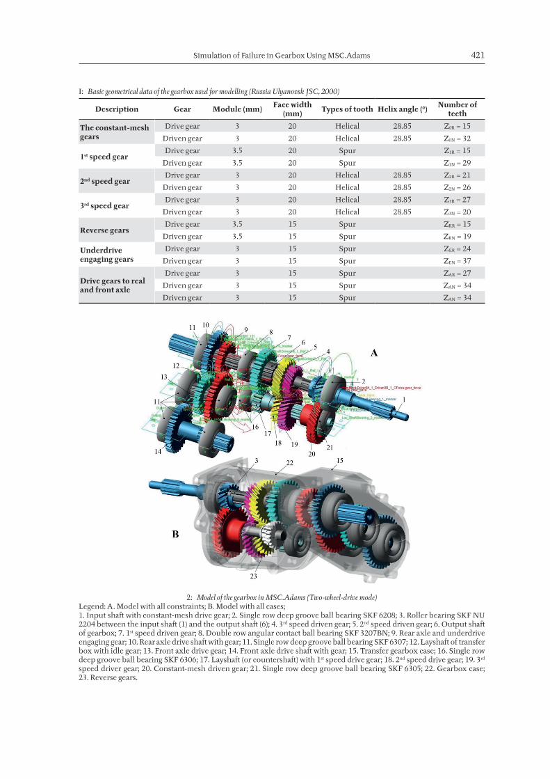
2: Model of the gearbox in MSC.Adams (Two-wheel-drive mode)Legend: A. Model with all constraints; B. Model with all cases; 1. Input shaft with constant‑mesh drive gear; 2. Single row deep groove ball bearing SKF 6208; 3. Roller bearing SKF NU 2204 between the input shaft (1) and the output shaft (6); 4. 3rd speed driven gear; 5. 2nd speed driven gear; 6. Output shaft of gearbox; 7. 1st speed driven gear; 8. Double row angular contact ball bearing SKF 3207BN; 9. Rear axle and underdrive engaging gear; 10. Rear axle drive shaft with gear; 11. Single row deep groove ball bearing SKF 6307; 12. Layshaft of transfer box with idle gear; 13. Front axle drive gear; 14. Front axle drive shaft with gear; 15. Transfer gearbox case; 16. Single row deep groove ball bearing SKF 6306; 17. Layshaft (or countershaft) with 1st speed drive gear; 18. 2nd speed drive gear; 19. 3rd speed driver gear; 20. Constant‑mesh driven gear; 21. Single row deep groove ball bearing SKF 6305; 22. Gearbox case; 23. Reverse gears.


When the gearbox model is imported with the above method, each component stands by itself in MSC.Adams and has no connection with another one. Because of this, they will not constitute a real virtual model and will not work as required. Next, two procedures need to be fulfilled: a) Adding material parameters, so that the physical

data of gears and shafts such as centroid position, mass, stiffness and the rotation inertia defined as equation (1), can be obtained (Norton and Karczub, 2003).

2

2 2

12

1(3 )

12

xx

yy zz

I mr

I I m r L

= = = +

(1)

Wherem .........mass of the components,r ...........radius of the components,L ..........width of the components,xx ........rotating axis,yy, zz ...perpendicular axes with rotating axis.

b) Adding torque and kinematic constraints. If the torque and the motion applied to the gears need to be transferred to the shaft, a fixed joint is added to every gear wheel and a corresponding shaft. A revolute and cylindrical joint is added to every shaft, so that it can rotate around its own axis. A constant rotational motion is applied to a revolute joint on the input shaft. This represents a virtual rotation from the engine and resistive torques which are applied on the output shafts as load from the axles. All the SKF virtual bearings, which were chosen on the basis of the equivalent parameters of the real Russian bearings, are also added to the model (see Fig. 2).

Determination of the contact force parameters

Although numerous variants of gears dynamics modelling can be considered, we selected the approach that takes into account the phenomena occurring only inside a gearbox. This approach is used for calculating dynamic contact forces between teeth. By doing so, it can identify the signs of teeth failures. Meshing stiffness, which depends on the number of intermeshing teeth and the deflection

of a tooth by load during meshing, varies in time in real gears and is theoretically changed according to a parabolic function and determined by parameters of contact algorithm.

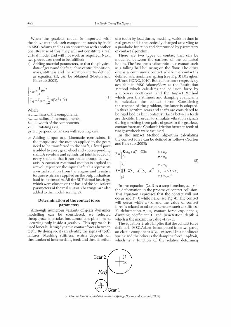
There are two types of contact that can be modelled between the surfaces of the contacted bodies. The first one is a discontinuous contact such as a falling ball bouncing on the floor. The other one is a continuous contact where the contact is defined as a nonlinear spring (see Fig. 3) (Meagher, WU and KONG, 2010). Both of them are respectively available in MSC.Adams/View as the Restitution Method which calculates the collision force by a recovery coefficient, and the Impact Method which uses the stiffness and damping coefficients to calculate the contact force. Considering the essence of the problem, the latter is adopted. In this algorithm gears and shafts are considered to be rigid bodies but contact surfaces between teeth are flexible. In order to simulate vibration signals during meshing from pairs of gears in the gearbox, contact force and Coulomb friction between teeth of two gear wheels were assumed.

In the Impact Method algorithm calculating the contact force can be defined as follows (Norton and Karczub, 2003):

0( )

0

eK x x CSxF

+ +=

0

0

x x

x x

<≥

[ ] 20 0

0

3 2( ) ( )

1

S x x x x

= − − −

0

0 0

0

x x

x d x x

x x d

>

− < <

≤ −

(2)

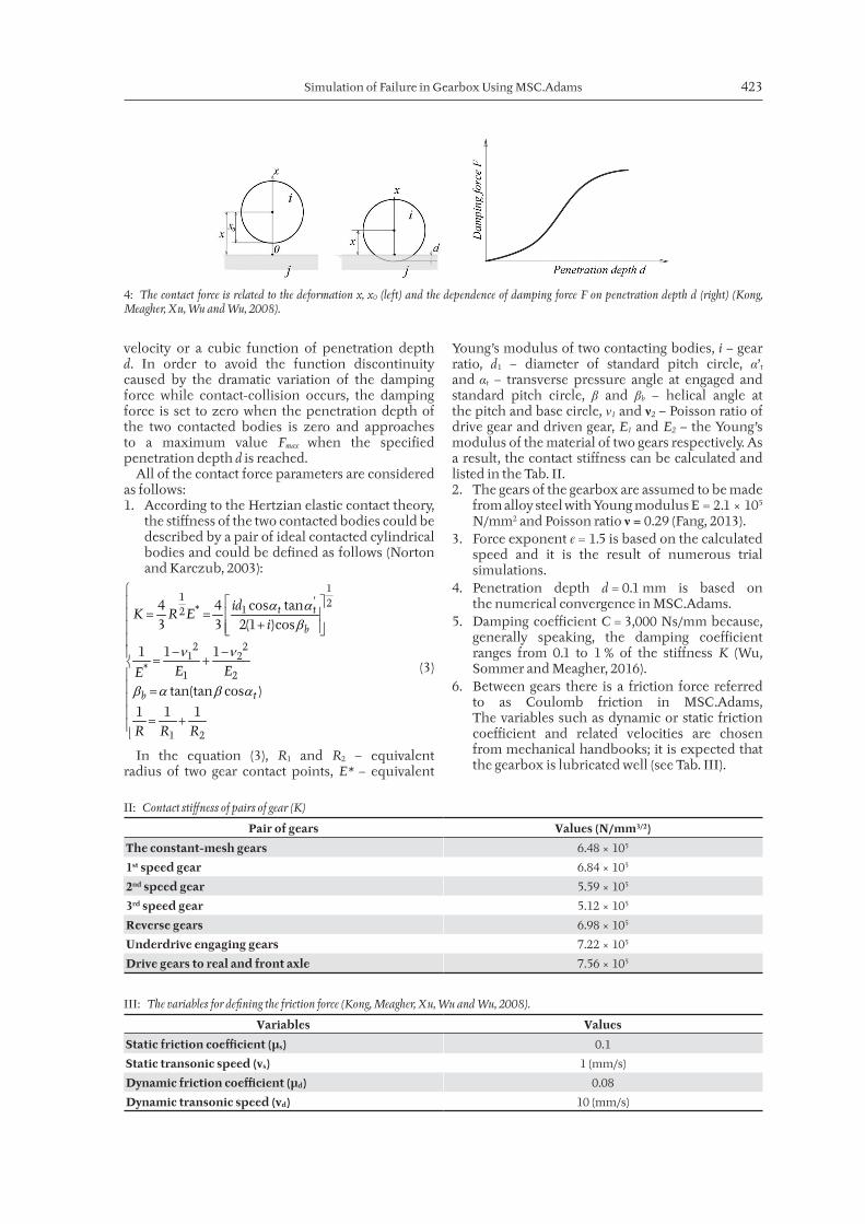
In the equation (2), S is a step function, x0 − x is the deformation in the process of contact‑collision. This equation expresses that the contact will not occur and F = 0 while x ≥ x0 (see Fig. 4). The contact will occur while x < x0 and the value of contact force is related to other parameters such as stiffness K, deformation x0 − x, contact force exponent e, damping coefficient C and penetration depth d which is the maximum value of x0 − x.

The equation (2) also implies that the contact force defined in MSC.Adams is composed from two parts, an elastic component K(x0 − x)e acts like a nonlinear spring and the other is the damping force CS(dx / dt) which is a function of the relative deforming

3: Contact force is defined as a nonlinear spring (Norton and Karczub, 2003).


velocity or a cubic function of penetration depth d. In order to avoid the function discontinuity caused by the dramatic variation of the damping force while contact‑collision occurs, the damping force is set to zero when the penetration depth of the two contacted bodies is zero and approaches to a maximum value Fmax when the specified penetration depth d is reached.

All of the contact force parameters are considered as follows:1. According to the Hertzian elastic contact theory,

the stiffness of the two contacted bodies could be described by a pair of ideal contacted cylindrical bodies and could be defined as follows (Norton and Karczub, 2003):

11 ' 2* 12

2 21 2

*1 2

1 2

4 4 cos tan3 3 2(1 )cos

1 1 1

tan(tan cos )

1 1 1

t t

b

tb

idK R E

i

E EE

R R R

α αβ

ν ν

β α β α

= = +

− − = +

= = +

(3)

In the equation (3), R1 and R2 – equivalent radius of two gear contact points, E* – equivalent

Young’s modulus of two contacting bodies, i – gear ratio, d1 – diameter of standard pitch circle, α’t

and αt – transverse pressure angle at engaged and standard pitch circle, β and βb – helical angle at the pitch and base circle, ν1 and ν2 – Poisson ratio of drive gear and driven gear, E1 and E2 – the Young’s modulus of the material of two gears respectively. As a result, the contact stiffness can be calculated and listed in the Tab. II.2. The gears of the gearbox are assumed to be made

from alloy steel with Young modulus E = 2.1 × 105 N/mm2 and Poisson ratio ν = 0.29 (Fang, 2013).

3. Force exponent e = 1.5 is based on the calculated speed and it is the result of numerous trial simulations.

4. Penetration depth d = 0.1 mm is based on the numerical convergence in MSC.Adams.

5. Damping coefficient C = 3,000 Ns/mm because, generally speaking, the damping coefficient ranges from 0.1 to 1 % of the stiffness K (Wu, Sommer and Meagher, 2016).

6. Between gears there is a friction force referred to as Coulomb friction in MSC.Adams, The variables such as dynamic or static friction coefficient and related velocities are chosen from mechanical handbooks; it is expected that the gearbox is lubricated well (see Tab. III).

4: The contact force is related to the deformation x, x0 (left) and the dependence of damping force F on penetration depth d (right) (Kong, Meagher, Xu, Wu and Wu, 2008).

II: Contact stiffness of pairs of gear (K)

Pair of gears Values (N/mm3/2)

The constant-mesh gears 6.48 × 105

1st speed gear 6.84 × 105

2nd speed gear 5.59 × 105

3rd speed gear 5.12 × 105

Reverse gears 6.98 × 105

Underdrive engaging gears 7.22 × 105

Drive gears to real and front axle 7.56 × 105

III: The variables for defining the friction force (Kong, Meagher, Xu, Wu and Wu, 2008).

Variables Values

Static friction coefficient (µs) 0.1

Static transonic speed (vs) 1 (mm/s)

Dynamic friction coefficient (µd) 0.08

Dynamic transonic speed (vd) 10 (mm/s)


Algorithms for the dynamic simulationMSC.Adams offers four solvers (the Gstiff,

Wstiff, Dstiff and Constant‑BDF) to solve the Differential‑Algebra Equation (DAE) for the multi‑body dynamic simulation. All of them use multi‑step, variable order algorithms and apply one of these three integration formats including the Index3 (I3), Stabilized Index 1 (SI1) and Stabilized Index 2 (SI2).

The Gstiff and the Wstiff use a variable step and fixed coefficients. The former helps us to calculate faster with higher accuracy, but when computing velocity, they can make an error which might excite discontinuities in acceleration. Because of this, the error must be controlled by limiting the maximum step during the simulation. The latter is more useful and stable because it could be modified according to variable steps without any accuracy loss, but it requires more calculated time than those by the Gstiff. The Dstiff algorithm is similar to the Wstiff, but it allows us to choose only the integration format Index3. Unlike them, the Constant‑BDF algorithm uses fixed steps, so it is very useful when SI2 format is selected with short step. Although it does not calculate as fast as the Gstiff and Wstiff, it also reaches high accuracy and it is not as sensitive to the discontinuity of the acceleration and force as the Gstiff (Mechanical Dynamics, 2008).

Integration formats differ a lot, for instance the I3 monitors only the error of the displacement and other state variables of the differential equations, but not the velocities and constrained reaction forces. Therefore, its accuracy when calculating velocities, acceleration and constrained reaction forces is not as high as that of the others. The SI1 is able to monitor all state variables such as displacement, velocity and Lagrange multiplier by introducing the velocity constrained equations instead of acceleration constrained equations. Therefore, it calculates quite accurately but it is very sensitive to the models with friction and contact problems. Unlike the SI1, the SI2 is able to control the errors of the Lagrange multiplier and velocity by considering the velocity constrained equations, so more accurate result could be obtained for the velocity and acceleration computation.

Based on the above information about the solvers and integration formats, the Wstiff solver with SI2 integration is adopted for the dynamic simulation of the gearbox.

Algorithms analysing the contact forceBecause the function of contact force is periodic,

a Fourier transform (FFT) will be used to decompose it into a sum of simple harmonic functions, namely sines and cosines. Theoretically, the FFT can be defined as follows (Bakir, 2008 ):

01

2 2( ) ( cos sin )n n

n

nt ntx t a a b

T Tπ π∞

== + +∑ (4)

where x(t) is the function of contact force with period T, an and bn are constants called the coefficients of the transform and given by the Euler formulas (Bakir, 2008 ):

/2

0/2

1( )

T

T

a x t dxT −

= ∫ (5)

/2

/2

2 2( )cos

T

nT

nta x t dt

T Tπ

−

= ∫ n = 1, 2, … (6)

/2

/2

2 2( )sin

T

nT

ntb x t dt

T Tπ

−

= ∫ n = 1, 2, … (7)

However, in practice, the function of contact force is a set of data with discrete and finite values xn (n = 1, 2, …). To perform the analysis using these finite values of discrete data, the discrete Fourier transform (DFT) should be applied (Bakir, 2008 ):

12 /

0

1 Nj nk N

n kk

X x eN

π−

−

== ∑ n = 0,1,2 …N−1 (8)

where N is the number of xn in a constant interval Δt and Xn is called DFT of the discrete values x0, x1 … xN−1. Equation (8) will transfer correspondingly finite values on the time axis to the discrete spectra on the frequency axis. DFT can also use real numbers instead of complex ones (Bakir, 2008 ):

1

01

0

1 2cos

1 2sin

N

n kk

N

n kk

nkA x

N N

nkB x

N N

π

π

−

=−

=

=

=

∑

∑ n = 0,1,2….N−1 (9)

where Xn = An+jBn.We apply a window function in the work in

order to provide the discrete values that appear to be continuous and periodic. Discontinuities are “filled in” by forcing the function of contact force to be equal to zero at the beginning and the end of the calculated period.

There are many available windowing functions such as Rectangular (it is equivalent to saying that no window was used), Gaussian, Hamming, Blackman‑Harris and Hanning. If N is used to represent the width of a signal sample, these windows w[n] are defined in the range 0 ≤ n ≤ N − 1 as (note that outside 0 ≤ n ≤ N − 1 then w[n] = 0 for all cases) (Chitode, 2008):Rectangular window:

w[n]=1, 0; (10)

Hanning window:

2[ ] 0,5 0,5cos

nw n

Nπ

= − ; (11)

Hamming window:

2[ ] 0,54 0,46cos

nw n

Nπ

= − ; (12)


Gaussian:

22[ ] exp[ 0,5 ]

nw n

Nπ = −

; (13)

Blackman‑Harris window:

2 4[ ] 0,423 0,498cos 0,0792cos

n nw n

N Nπ π

= − + . (14)

After many times of trial calculation, Blackman‑Harris windowing function is used for the work.

The operating conditions of the gearbox during the simulation

The gearbox is used to transfer the engine power and the moment to the axles of the vehicle. In the process of operation it could suffer from heavy stimulation of the engine, the axles, the clutch and other resources such as oil, backlash, clearance. The stimulation makes the changes of the dynamic load very complex which is the main reason of vibrations, impact, noise and other signs. The selected operating conditions are based on the working characteristic of the gearbox in the field and they are among the huge number of possible choices which can be applied to the virtual gearbox.• Rotation speed n = 1,500 rpm is applied on

the input shaft (Fig. 2 position 1). • Position of 3rd speed gear (i = 1.58) is chosen in

the gearbox and two‑wheel‑drive mode is chosen in the transfer box.

• Load torque can be calculated from the maximum torque of the engine used on the vehicle (166.7 Nm) and the respective ratio (i = 1.58), then the load torques of 263.386 Nm is applied on the output shaft (Fig. 2 position 6).

• Other parameters are applied as follows: the simulation time (end time) 1 s and the simulation step (step size) 0.0001 s.

RESULTS AND DISCUSSION

Gear mesh frequencies (GMF)The gear mesh frequency also called “tooth mesh

frequency” is the rate at which gear teeth mesh together in a gearbox. It is equal to the number of teeth on the gear times the rotation speed of the gear (Norton and Karczub, 2003):

fm = f.Z, (15)

where fm is the gear mesh frequency (Hz), f is rotational frequency of the gear (Hz) and Z is the number of teeth.

The number of teeth on the drive gear times the speed of the drive gear must equal the number of teeth on the driven gear times the speed of the driven gear. As the pinion rotates against the driven gear, the individual cycles of the frequency generated are a profile of the individual teeth meshing. Gear mesh frequencies of gears in the gearbox were calculated as follows (see Tab. IV):

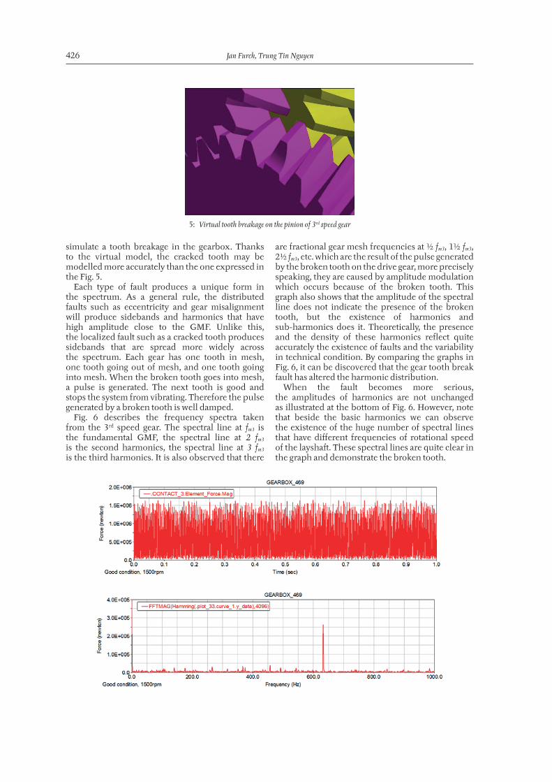
Simulation results of gear teeth contact forceThe top of Fig. 6 shows the graph of the gear teeth

contact force for the pair of 3rd speed gears under normal conditions.

It is easily observed that the above results seem to fit the theoretical values (in Tab. IV) well. Note that values of the GMF are always repeated with an integer multiplier also known as harmonics. The second and the third harmonics are very important. In the spectrum of 3rd speed gears (see top of Fig. 6), the second harmonics of GMF (2fm3) has a high amplitude with respect to the fundamental (fm3) and the third harmonics (3fm3) which would indicate a backlash‑type problem. In other words, the gears may have too much backlash, or one of the gears may be oscillating. It is known that there are 4 pairs of gears used to transfer power from the input shaft to the layshaft and the outshaft (see Fig. 2), but not all of them can have the same perfect mesh condition. In either cases, the gears are meshing on both sides of the teeth. This double mesh generates the second harmonics, the phase of which is 1800 out of the phase with the fundamental.

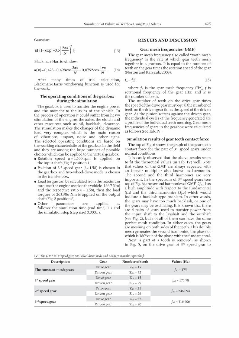
Next, a part of a tooth is removed, as shown in Fig. 5, on the drive gear of 3rd speed gear to

IV: The GMF in 3rd speed gear, two-wheel-drive mode and 1,500 rpm on the input shaft

Description Gear Number of teeth Values (Hz)

The constant-mesh gearsDrive gear Z0R = 15

fm0 = 375Driven gear Z0N = 32

1st speed gearDrive gear Z1R = 15

fm1 = 175.78Driven gear Z1N = 29

2nd speed gearDrive gear Z2R = 21


3rd speed gearDrive gear Z3R = 27



simulate a tooth breakage in the gearbox. Thanks to the virtual model, the cracked tooth may be modelled more accurately than the one expressed in the Fig. 5.

Each type of fault produces a unique form in the spectrum. As a general rule, the distributed faults such as eccentricity and gear misalignment will produce sidebands and harmonics that have high amplitude close to the GMF. Unlike this, the localized fault such as a cracked tooth produces sidebands that are spread more widely across the spectrum. Each gear has one tooth in mesh, one tooth going out of mesh, and one tooth going into mesh. When the broken tooth goes into mesh, a pulse is generated. The next tooth is good and stops the system from vibrating. Therefore the pulse generated by a broken tooth is well damped.

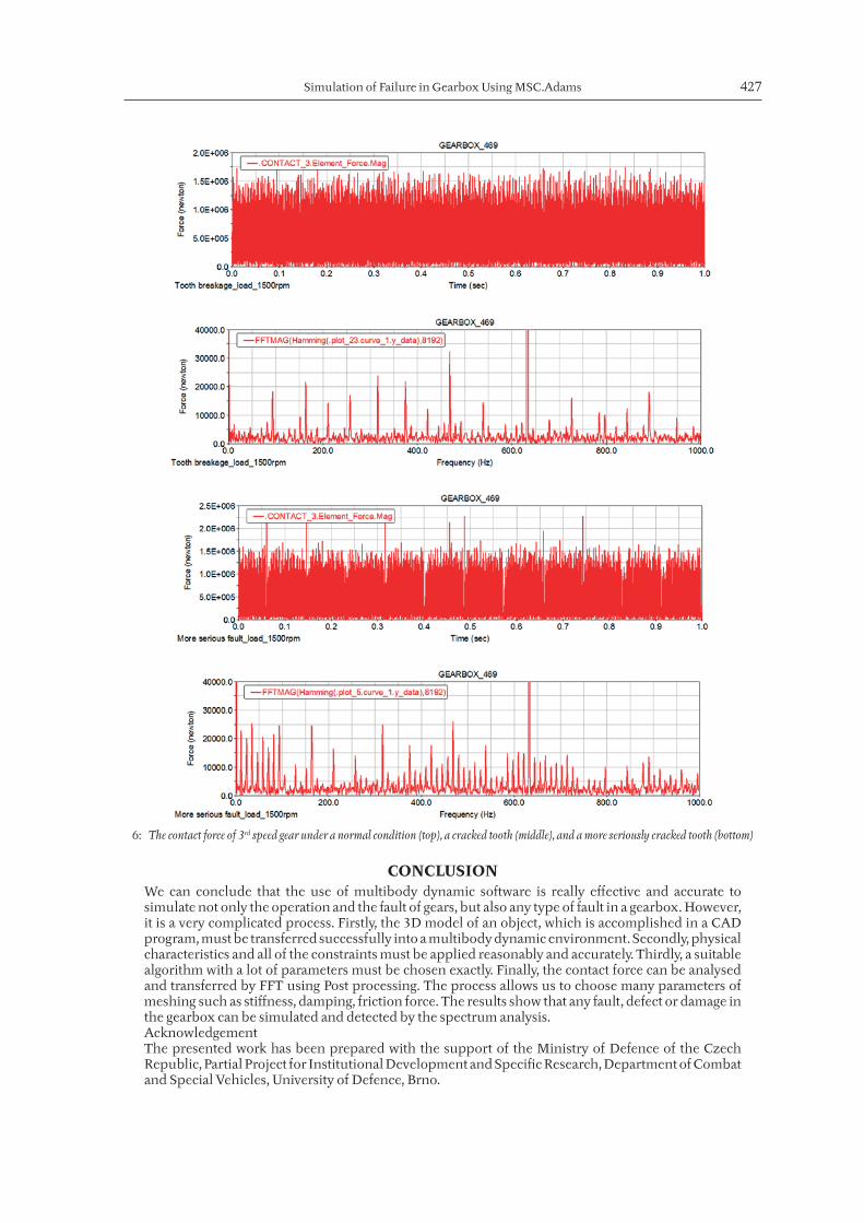
Fig. 6 describes the frequency spectra taken from the 3rd speed gear. The spectral line at fm3 is the fundamental GMF, the spectral line at 2 fm3 is the second harmonics, the spectral line at 3 fm3 is the third harmonics. It is also observed that there

are fractional gear mesh frequencies at ½ fm3, 1½ fm3, 2½ fm3, etc. which are the result of the pulse generated by the broken tooth on the drive gear, more precisely speaking, they are caused by amplitude modulation which occurs because of the broken tooth. This graph also shows that the amplitude of the spectral line does not indicate the presence of the broken tooth, but the existence of harmonics and sub‑harmonics does it. Theoretically, the presence and the density of these harmonics reflect quite accurately the existence of faults and the variability in technical condition. By comparing the graphs in Fig. 6, it can be discovered that the gear tooth break fault has altered the harmonic distribution.

When the fault becomes more serious, the amplitudes of harmonics are not unchanged as illustrated at the bottom of Fig. 6. However, note that beside the basic harmonics we can observe the existence of the huge number of spectral lines that have different frequencies of rotational speed of the layshaft. These spectral lines are quite clear in the graph and demonstrate the broken tooth.

5: Virtual tooth breakage on the pinion of 3rd speed gear


CONCLUSIONWe can conclude that the use of multibody dynamic software is really effective and accurate to simulate not only the operation and the fault of gears, but also any type of fault in a gearbox. However, it is a very complicated process. Firstly, the 3D model of an object, which is accomplished in a CAD program, must be transferred successfully into a multibody dynamic environment. Secondly, physical characteristics and all of the constraints must be applied reasonably and accurately. Thirdly, a suitable algorithm with a lot of parameters must be chosen exactly. Finally, the contact force can be analysed and transferred by FFT using Post processing. The process allows us to choose many parameters of meshing such as stiffness, damping, friction force. The results show that any fault, defect or damage in the gearbox can be simulated and detected by the spectrum analysis.AcknowledgementThe presented work has been prepared with the support of the Ministry of Defence of the Czech Republic, Partial Project for Institutional Development and Specific Research, Department of Combat and Special Vehicles, University of Defence, Brno.

6: The contact force of 3rd speed gear under a normal condition (top), a cracked tooth (middle), and a more seriously cracked tooth (bottom)


REFERENCESBAKIR, P. G. 2008. Vibration based structural health monitoring. Berlin: Technische Universitat Berlin. CHITODE, J. S. 2008. Digital signal processing. 1st Edition. Pune: Technical Publications Pune. DABROWSKI, D., ADAMCZYK, J. and PLASCENCIA, H. 2012. A Multi‑model of gears for simulation of

vibration signals for gears misalignment. Diagnostyka- Applied structural health, usage and condition monitoring, 62(2): 15 – 22.

FANG, B. 2013. CAE Methods on Vibration-based Health Monitoring of Power Transmission Systems. San Luis Obispo: California Polytechnic State University.

FURCH, J., GLOS, J. and NGUYEN, T. T. 2016. Vibration analysis of manual transmission using physical simulation. In: Deterioration Dependalility Diagnostics. Brno, 11 – 12 October. Brno: University of Defence, 57 – 68.

FURCH, J., GLOS, J. and NGUYEN, T. T. 2016. Modelling and simulation of mechanical gearbox vibrations. In: International scientific conference Transport means 2016. Juodkrante, 5 – 7 October. Kaunas: Kaunas University of Technology, vol. 1, 133 – 139.

MEAGHER, J., WU, X. and KONG, D. 2010. A Comparison of Gear Mesh Stiffness Modeling Strategies. In: Proceedings of the IMAC – XXVIII. Jacksonville: Society for Experimental Mechanics Inc.

MECHANICAL DYNAMICS. 2000. Building Models in ADAMS/View. Michigan: Mechanical Dynamics.NORTON. M. P. and KARCZUB. D. G. 2003. Fundamentals of Noise and Vibration Analysis for Engineers. 2nd edition.

Cambridge: Cambridge University Press.NOVOTNÝ, P., PROKOP, A., ZUBÍK, M. and ŘEHÁK, K. 2016. Investigating the influence of computational

model complexity on noise and vibration modeling of powertrain. Journal of Vibroengineering, 22(4): 378 – 393.RUSSIA ULYANOVSK JSC. 2000. Automobiles UAZ-31512, UAZ-31514, UAZ-31519, Parts Catalogue.

Ulyanovsk: JSC UAZ.KONG, D., MEAGHER, J. M., XU, C., WU, X., and WU, Y. 2008. Nonlinear Contact Analysis of Gear Teeth

for Malfunction Diagnostics. In: IMAC XXVI Conference and Exposition on Structural Dynamics. Orlando, 4 February. Bethel: Society for Experimental Mechanics.

WU, X., SOMMER, A. and MEAGHER, J. 2016. Spectrum Diagnostics of a Damaged Differential Planetary Gear during Various Operating Conditions. Physical Science International Journal, 9(3): 1 – 13.

Contact information

Jan Furch: [email protected] Tin Nguyen: [email protected]

Documents

SIMULATION OF FAILURE IN GEARBOX USING MSC · PDF fileSIMULATION OF FAILURE IN GEARBOX USING MSC.ADAMS ... Keywords: gearbox, cracked tooth, simulation, model, vibration signal, contact