Simulation of Dilute Acetone Spray Flames with LES-CMC Using Two Conditional Moments

Flow Turbulence Combust (2014) 93:405–423DOI 10.1007/s10494-014-9565-1

Simulation of Dilute Acetone Spray Flameswith LES-CMC Using Two Conditional Moments

Satoshi Ukai ·Andreas Kronenburg ·Oliver T. Stein

Received: 18 December 2013 / Accepted: 30 July 2014 / Published online: 13 August 2014© Springer Science+Business Media Dordrecht 2014

Abstract Large-eddy simulations (LES) have been coupled with a conditional moment clo-sure (CMC) method for the computation of a series of turbulent spray flames. An earlierstudy by Ukai et al. (Proc. Combust. Inst. 34(1),1643–1650, 2013) gave reasonable resultsfor the prediction of temperature and velocity profiles, but some limitations of the methodbecame apparent. These limitations are primarily related to the upper limit in mixture frac-tion space. In order to enhance the applicability of the LES-CMC model, this paper proposesa two-conditional moment approach to account for the existence of pre-evaporated fuel byintroducing two sets of conditional moments based on different mixture fractions. The two-conditional moment approach is first tested for a non-reacting test case. The results indicatethat the spray evaporation induces relatively large conditional fluctuations within a CMCcell, and one set of conditional moments might not be sufficient. The upper limit of the mix-ture fraction space is dynamically selected for the solution of the second set of conditionalmoments, and the corresponding CMC solution in a CFD cell is estimated by interpolationbetween the two conditional moments weighted by the amount of vapour emitted withinthe domain. The cell-filtered value is given by integration of the conditional moment acrossmixture fraction space using a bounded β-FDF for the distribution of the scalar. As a result,the fuel concentration profiles given by LES and the two-conditional moment approachare shown to agree well. Then, the two-conditional moment approach is applied to fourdifferent flame configurations. The comparison of LES cell quantities and conditionallyaveraged moments indicates that the two sets of conditional moments are necessary foraccurate predictions in zones where gas phase mixture fraction is significantly increasedby droplet evaporation within the computational domain. The unconditional temperatureprofiles clearly show that the new approach improves the predictions of mean temperatureespecially along the centerline. Also, the better predictions of the temperature field improvethe accuracy of the predicted mean axial droplet velocities. Overall, good agreement withthe experimental results is found for all four cases, and the methodology is shown to beapplicable to flames with a relatively wide range of fuel vapour concentrations.

S. Ukai · A. Kronenburg (�) · O. T. SteinInstitut fur Technische Verbrennung, Universitat Stuttgart, 70174 Stuttgart, Germanye-mail: [email protected]

mailto:[email protected]

406 Flow Turbulence Combust (2014) 93:405–423

Keywords CMC · LES · Spray · Evaporation · Combustion

1 Introduction

Many industrial combustion systems involve turbulent spray flames. A crucial aspect ofthese flames is the effect of turbulence on the spray and combustion chemistry [1]. Large-eddy simulation (LES) has been well recognized due to its ability to resolve unsteady flowstructures and mixing processes. However, LES of turbulent combustion still requires asubgrid model for a chemical reaction, since its characteristic scales are often smaller thanan LES cell size. There have been various types of turbulent combustion models proposedincluding the Flamelet approach [2–5], the PDF model [6], the linear-eddy model [7], theEulerian stochastic field method [8], the MMC [9] and the conditional moment closure(CMC) [10]. We use an LES-CMC formulation in this study, since it has been thoroughlyvalidated for many types of flame configurations such as piloted flames [10, 11], bluff-bodyflames [12] and lifted flames [13–16]. Also, a Lagrangian scheme to compute the dropletproperties is often coupled with the LES of the gas phase quantities. The effects of subgridfluctuations on the droplets are usually included by the use of stochastic dispersion andevaporation models [17, 18].

The simulation of spray flame needs to consider the interactions of turbulence, the sprayand the chemistry, and their accurate modelling may be crucial for the quality of the pre-dictions. Spray flames have been simulated by using the single phase CMC equations inRANS [19, 20] and LES [21] and simplified spray CMC formulations in RANS [22, 23].Mortensen and Bilger [24] mathematically derived extra terms within the CMC equationsfor spray combustion, and the effects of the term may not be negligible. The new spray CMCequations have been applied successfully to turbulent spray flames in auto-ignition studies[25, 26] where one conditional moment can sufficiently approximate the correct solution.Ukai et al. [27] applied two-phase LES-CMC to a dilute acetone spray jet flame with pre-evaporation for the first time, and discussed the impact of the additional spray terms. Thestudy pointed out difficulties with the selection of an appropriate upper limit of mixturefraction, ξU , due to the effect of evaporation. In general, a single-phase CMC implementa-tion (or non-premixed approaches in general) assumes ξU to be fixed at the fuel condition.In liquid fuel combustion, ξU could represent the gas phase value at the liquid-gaseous inter-face, however, the maximum mixture fraction varies in space and time on a sub-grid scaledue to varying droplet temperatures, and it is difficult to define a single ξU and correspond-ing boundary conditions for the depending scalars that are applicable throughout the entiredomain. One compromise applied in the previous study [27] is to fix ξU at the fuel jet mix-ture fraction ξjet originating from pre-evaporation inside the jet nozzle. This approach ledto a good match of the predictions with experiments near the jet inlet where most of theevaporation occurs without any mixing with the surrounding streams. However, the assump-tion is not fully valid where droplet vapour and oxidizer are mixed more homogeneously,and, as a result, predicted temperatures were much below the experimental data along thecenterline further downstream. An alternative approach is to adjust ξU dynamically basedon the mixing fields, and better predictions can be expected downstream. Now, ξU does nolonger equal a maximum (sub-grid) mixture fraction value at a droplet surface, it rather rep-resents a suitable upper bound in mixture fraction space and the upper bound of the mixturefraction distribution. Note, however, that a dynamically moving ξU may not be sufficientfor accurate CMC modelling of spray flames with pre-evaporation, since scalar dissipa-tion can cause unphysical mixing in the jet core where mixing with the surrounding flow

Flow Turbulence Combust (2014) 93:405–423 407

should not occur. Thus, a new method must be developed to treat evaporating sprays moreappropriately.

The current study aims to develop and validate a two-conditional moment approach for aspray flame that can deal with a shift of ξU dynamically. First, we discuss difficulties asso-ciated with modelling pre-evaporated spray flames by using a non-reacting t case with anevaporating spray, and the effect of the two-conditional moment approach is analyzed. Then,the two-conditional moment approach is applied to dilute acetone spray flames with pre-evaporation. Our test cases are selected from the well defined experiments carried by Masriand Gounder [28] as a part of the Workshop on Measurement and Computation of TurbulentSpray Combustion (TCS) [29]. They have performed parametric studies of spray flames bychanging mass flow rates and liquid injection rates for two species: acetone and ethanol.Different numerical studies of the these flames have been accomplished by using CMC[27], flamelet generated manifoldis (FGM) [30–32], a flamelet progress Variable approachwith a fully stochastic separated flow (FSSF) approach for droplets [33] and a probabilitydensity function approach [34]. Because the CMC methodology is based on a mixture frac-tion concept, it is –strictly speaking– only applicable to spray flames that do not burn inthe premixed combustion mode. This would be true for spray with very little or very largeamounts of pre-evaporation where conditions at the jet exit are not within the flammabilitylimits. Thus, the four cases chosen here include spray jets with relatively large degrees ofpre-evaporation.

2 Gas and Liquid Phase Formulations

LES solves spatially filtered equations with a modelling of subgrid scale effects. The Favre-filtered continuity and momentum equations read

∂ρ

∂t+ ∂

∂xj(ρuj ) = ¯ρ, (1)

∂

∂t(ρui)+ ∂

∂xj(ρui uj ) = − ∂p

∂xi+ ∂ τij

∂xj− ∂τ

sgsij

∂xj+ ¯Fi, (2)

where ρ is density, ui are the velocities in i direction, p is pressure and τ denotes the viscous

stress tensor, ¯ρ, ¯Fi are the source terms for mass and momentum that can be associated withthe liquid phase, τ sgsij is the subgrid stress tensor. A dynamic subgrid eddy viscosity model

is used to model τ sgsij [35].Mixture fraction is a useful concept to analyze non-premixed flames. The mixture frac-

tion is usually set to unity in the fuel stream, and the maximum mixture fraction withinthe domain is kept less than or equal to 1.0. However, in turbulent spray flames, the maxi-mum mixture fraction can exceed the value associated with the gaseous fuel jet at the inlet.We therefore suggest to solve transport equations for two mixture fraction simultaneously:the total mixture fraction, ξtot , and the conserved mixture fraction, ξcons . ξtot representsthe mixture fraction associated with the inlet conditions (a pilot flame and fuel originatingfrom pre-evaporated droplets that lead to fuel vapour at the jet exit) and the fuel originatingfrom droplet evaporation within the domain. ξcons is based on the fuel from pre-evaporationwithin the nozzle and the fuel elements of the pilot flame only. ξcons is not affected by thefuel evaporating from the droplets within the domain. Solving these two mixture fractions,the mixture fraction evaporated from the droplets after exiting the nozzle can be computedas ξ� = ξtot − ξcons , and it plays an important role in the following modelling approach.


The maximum value of ξtot changes dynamically and is defined to be unity when the mix-ture is pure fuel. The maximum value of ξcons corresponds to the maximum inlet mixturefraction. The Favre-filtered scalar transport equations for the two mixture fractions are

∂

∂t(ρξtot )+ ∂

∂xj(ρuj ξtot ) = −∂Jtot

∂xj− ∂J

sgstot

∂xj+ ¯ξ, (3)

∂

∂t(ρξcons)+ ∂

∂xj(ρuj ξcons) = −∂Jcons

∂xj− ∂J

sgscons

∂xj, (4)

where J is the diffusion flux of mixture fraction, ¯ξ is the source term of the mixturefraction due to evaporation within the domain, and J sgs is the subgrid diffusion term. ASIMPLE-type predictor-corrector procedure [36] is used to solve the governing equations.A Lagrangian particle tracking scheme is used to track individual spray droplets. Position,velocity, temperature and evaporation rate of each droplet are calculated and additionalfluctuation terms are included to account for sub-grid effects [17].

3 Conditional Moment Closure

The CMC equations are formulated to solve for the conditionally averaged reactive scalars.The conditional moment of the species α is defined as Qα(ξ,x, t) ≡ 〈Yα(x, t)|ξ(x, t) = η〉,and it is often assumed that the conditional fluctuations within the flow are relatively small.However, in practice, the conditional fluctuation can be very large for spray flames, and itmight be inaccurate to represent the properties by only one conditional moment as discussedin Section 5. Therefore, two sets of conditional moments conditioned on ξcons and ξtotare solved simultaneously, and the solution is obtained by interpolation between the twoconditional moments as presented later. The conservative form of the CMC equation for theconditional moment conditioned on ξcons is

∂

∂tQα,cons + 1

ρη ˜Pη

∇ · [ρη ˜Pη

(

UηQα,cons −Dt,η∇Qα,cons

)]

= ωη,α +Nη∂2

∂η2Qα,cons + Qα,cons

ρη ˜Pη

∇ · (ρη ˜PηUη

)

, (5)

where subscript η denotes conditionally averaged quantities, N is the scalar dissipationrate, ωα is the chemical source term of species α, Dt is the turbulent diffusivity and P isthe probability density function. The subscript cons indicates conditioning on the randomvariable, ξcons . Note that all conditioned quantities in Eq. 5 are conditioned on ξcons , but thesubscripts are only shown for Qα,cons to preserve some clarity of presentation. The CMCequation for the moments conditionally averaged on ξtot includes additional spray sourceterms [24, 25] as

∂

∂tQα,tot + 1

ρη ˜Pη

∇ · [ρη ˜Pη

(

UηQα,tot −Dt,η∇Qα,tot

)]

= ωη,α +Nη

∂2

∂η2Qα,tot + Qα,tot

ρη ˜Pη


)

+[

Q1,α −Qα,tot − (1 − η)∂

∂ηQα,tot

]

�η, (6)


where Q1,α denotes the composition of the liquid fuel, � is the volumetric fuel evaporationrate. The subscript tot indicates conditioning on the random variable ξtot and all conditionalproperties in Eq. 6 are conditioned on ξtot . It follows from Eqs. 5 and 6 that the corre-sponding unconditional quantities (that can be recovered from the conditional moments byintegration across mixture fraction space) will also differ.

Similarly, the conditionally averaged enthalpy equations are given by

∂

∂tQh,cons + 1

ρη,cons ˜Pη

∇ · [ρη ˜Pη

(

UηQh,cons −Dt,η∇Qh,cons

)]

= Nη∂2

∂η2Qh,cons + Qh,cons

ρη ˜Pη


) + erad,η, (7)

and∂

∂tQh,tot + 1

ρη ˜Pη

∇ · [ρη ˜Pη

(

UηQh,tot −Dt,η∇Qh,tot

)]

= Nη

∂2

∂η2Qh,tot + Qh,tot

ρη ˜Pη


)

+ erad,η +[

Q1,h −Qh,tot − (1 − η)∂

∂ηQh,tot

]

�η +�η, (8)

where Qh is the conditionally averaged enthalpy, erad is the radiation heat loss that is mod-elled assuming an optically thin flame [37], and � is the heat transfer term between the sprayand the gas phases. Unity Lewis numbers have been assumed. The modelling approaches forthe conditionally averaged quantities (�η, �η, Nη, Uη and Dt,η) are explained and discussedin our previous work [10, 27], and the current study takes that these terms are identical forboth the formulations of Qtot and Qcons . The terms ωη,α and erad,η are functions of eachconditional moment, (e.g. ωη,α,tot = f (Qα,η,tot , Tη,tot )), so that ωη,α,tot �= ωη,α,cons anderad,η,tot �= erad,η,cons .

4 Computational Configuration

The two-conditional moment approach is tested with four cases from a series of acetonespray flame experiments [28], and the selection of the configurations is motivated by theamount of pre-evaporation at the jet exit. The liquid fuel is seeded upstream of the noz-zle exit, and a certain portion of the liquid fuel evaporates and appears in the gaseousphase. Since the present CMC is an extension of a mixture fraction based approach fornon-premixed gaseous flames, the flame shall burn largely in non-premixed mode whichexcludes flames with very specific degrees of fuel pre-evaporation leading to mixture frac-tion values close to stoichiometric (ξst = 0.0955) at the jet exit. Therefore, the studyconsiders the four cases AcF 1, AcF 2, AcF 3 and AcF 5. Results for AcF 3 are comparedwith results from [27]. In addition, one simulation of an evaporating spray jet has been con-ducted for validation purposes. The setup of the (notional) non-reacting case has been basedon AcF 3. The inflow gas velocity and liquid fuel rates of the selected cases are listed inTable 1. The velocities of the pilot and the co-flow are 11.9 m/s and 4.5 m/s, respectively,and do not vary from case to case. The diameter of the jet, D, and the outer annulus diam-eter of the pilot and the co-flow are 10.5 mm, 25 mm and 104 mm, respectively. The inletcross-section is 10Dx10D and diverging towards the exit, and the domain length is taken tobe 40D. The LES grid size is 90 × 90 × 240, and the cells are clustered around the nozzle.


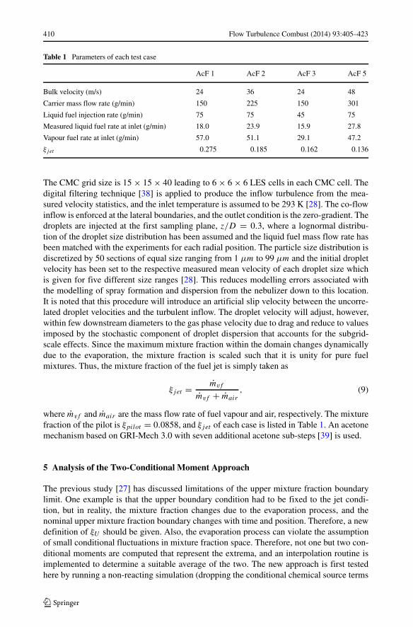
Table 1 Parameters of each test case

AcF 1 AcF 2 AcF 3 AcF 5

Bulk velocity (m/s) 24 36 24 48

Carrier mass flow rate (g/min) 150 225 150 301

Liquid fuel injection rate (g/min) 75 75 45 75

Measured liquid fuel rate at inlet (g/min) 18.0 23.9 15.9 27.8

Vapour fuel rate at inlet (g/min) 57.0 51.1 29.1 47.2

ξjet 0.275 0.185 0.162 0.136

The CMC grid size is 15 × 15 × 40 leading to 6 × 6 × 6 LES cells in each CMC cell. Thedigital filtering technique [38] is applied to produce the inflow turbulence from the mea-sured velocity statistics, and the inlet temperature is assumed to be 293 K [28]. The co-flowinflow is enforced at the lateral boundaries, and the outlet condition is the zero-gradient. Thedroplets are injected at the first sampling plane, z/D = 0.3, where a lognormal distribu-tion of the droplet size distribution has been assumed and the liquid fuel mass flow rate hasbeen matched with the experiments for each radial position. The particle size distribution isdiscretized by 50 sections of equal size ranging from 1 μm to 99 μm and the initial dropletvelocity has been set to the respective measured mean velocity of each droplet size whichis given for five different size ranges [28]. This reduces modelling errors associated withthe modelling of spray formation and dispersion from the nebulizer down to this location.It is noted that this procedure will introduce an artificial slip velocity between the uncorre-lated droplet velocities and the turbulent inflow. The droplet velocity will adjust, however,within few downstream diameters to the gas phase velocity due to drag and reduce to valuesimposed by the stochastic component of droplet dispersion that accounts for the subgrid-scale effects. Since the maximum mixture fraction within the domain changes dynamicallydue to the evaporation, the mixture fraction is scaled such that it is unity for pure fuelmixtures. Thus, the mixture fraction of the fuel jet is simply taken as

ξjet = mvf

mvf + mair

, (9)

where mvf and mair are the mass flow rate of fuel vapour and air, respectively. The mixturefraction of the pilot is ξpilot = 0.0858, and ξjet of each case is listed in Table 1. An acetonemechanism based on GRI-Mech 3.0 with seven additional acetone sub-steps [39] is used.

5 Analysis of the Two-Conditional Moment Approach

The previous study [27] has discussed limitations of the upper mixture fraction boundarylimit. One example is that the upper boundary condition had to be fixed to the jet condi-tion, but in reality, the mixture fraction changes due to the evaporation process, and thenominal upper mixture fraction boundary changes with time and position. Therefore, a newdefinition of ξU should be given. Also, the evaporation process can violate the assumptionof small conditional fluctuations in mixture fraction space. Therefore, not one but two con-ditional moments are computed that represent the extrema, and an interpolation routine isimplemented to determine a suitable average of the two. The new approach is first testedhere by running a non-reacting simulation (dropping the conditional chemical source terms


in Eqs. 5 and 6) based on AcF 3, but with an artificially enhanced evaporation rate for bet-ter visualization of the effects. In this non-reacting case acetone is a conserved scalar andhence, the LES-filtered values can be compared with the CMC solution, see Section 5.5. InSection 6, the new approach is applied to the acetone flame series.

5.1 Effect of LES-mixing on mixture fraction

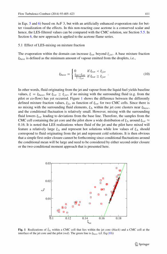
The evaporation within the domain can increase ξtot beyond ξjet . A base mixture fractionξbase is defined as the minimum amount of vapour emitted from the droplets, i.e.,

ξbase ={

0 if ξtot < ξjetξtot−ξjet1−ξjet

if ξtot ≥ ξjet. (10)

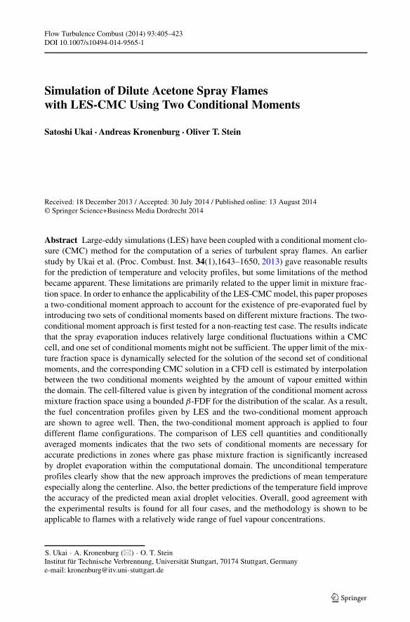
In other words, fluid originating from the jet and vapour from the liquid fuel yields baselinevalues, ξ = ξbase, for ξtot ≥ ξjet , if no mixing with the surrounding fluid (e.g. from thepilot or co-flow) has yet occurred. Figure 1 shows the difference between the differentlydefined mixture fraction values, ξ�, as function of ξtot for two CMC cells. Since there isno mixing with the surrounding fluid elements, ξ� within the jet core clusters near ξbase,and the conditional fluctuation is relatively small. However, mixing with the surroundingfluid lowers ξtot leading to deviations from the base line. Therefore, the samples from theCMC cell containing the jet core and the pilot show a wide distribution of ξ� around ξtot ≈0.16. It is noted that LES realizations where fluid of the jet and the pilot have mixed willfeature a relatively large ξ� and represent hot solutions while low values of ξ� shouldcorrespond to fluid originating from the jet and represent cold solutions. It is then obviousthat a simple first order closure cannot be forthcoming since conditional fluctuations aroundthe conditional mean will be large and need to be considered by either second order closureor the two-conditional moment approach that is presented here.

0.1 0.12 0.14 0.16 0.18ξ

tot

0

0.01

0.02

0.03

ξ Δ

Fig. 1 Realizations of ξ� within a CMC cell that lies within the jet core (black) and a CMC cell at theinterface of the jet core and the pilot (red). The green line is ξbase (cf. Eq.(10))


5.2 Selection of the upper mixture fraction boundary

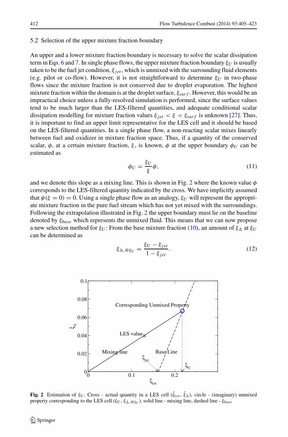
An upper and a lower mixture fraction boundary is necessary to solve the scalar dissipationterm in Eqs. 6 and 7. In single phase flows, the upper mixture fraction boundary ξU is usuallytaken to be the fuel jet condition, ξjet , which is unmixed with the surrounding fluid elements(e.g. pilot or co-flow). However, it is not straightforward to determine ξU in two-phaseflows since the mixture fraction is not conserved due to droplet evaporation. The highestmixture fraction within the domain is at the droplet surface, ξsurf . However, this would be animpractical choice unless a fully-resolved simulation is performed, since the surface valuestend to be much larger than the LES-filtered quantities, and adequate conditional scalardissipation modelling for mixture fraction values ξjet < ξ < ξsurf is unknown [27]. Thus,it is important to find an upper limit representative for the LES cell and it should be basedon the LES-filtered quantities. In a single phase flow, a non-reacting scalar mixes linearlybetween fuel and oxidizer in mixture fraction space. Thus, if a quantity of the conservedscalar, φ, at a certain mixture fraction, ξ , is known, φ at the upper boundary φU can beestimated as

φU = ξU

ξφ, (11)

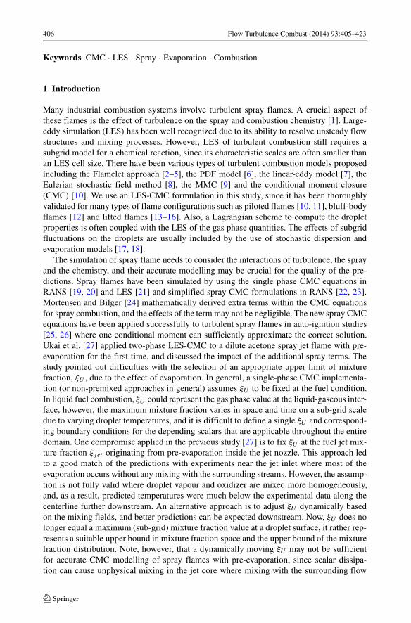
and we denote this slope as a mixing line. This is shown in Fig. 2 where the known value φcorresponds to the LES-filtered quantity indicated by the cross. We have implicitly assumedthat φ(ξ = 0) = 0. Using a single phase flow as an analogy, ξU will represent the appropri-ate mixture fraction in the pure fuel stream which has not yet mixed with the surroundings.Following the extrapolation illustrated in Fig. 2 the upper boundary must lie on the baselinedenoted by ξbase which represents the unmixed fluid. This means that we can now proposea new selection method for ξU : From the base mixture fraction (10), an amount of ξ� at ξUcan be determined as

ξ�,@ξU = ξU − ξjet

1 − ξjet. (12)

0 0.1 0.2ξ

tot

0

0.02

0.04

0.06

0.08

0.1

ξ Δ

Base LineMixing line

LES value

Corresponding Unmixed Property

ξU

ξjet

Fig. 2 Estimation of ξU . Cross - actual quantity in a LES cell (ξtot , ξ�), circle - (imaginary) unmixedproperty corresponding to the LES cell (ξU , ξ�,@ξU ), solid line - mixing line, dashed line - ξbase


Then, the linear mixing line (11) can be used to describe the mixing of ξ� by replacingφU = ξ�,@ξU , φ = ξ� and ξ = ξtot with xitot being the maximum value within one CMCcell.

ξ�,@ξU = ξU

ξtotξ�. (13)

Thus, ξU as the mixture fraction of the pseudo-unmixed fluid element is obtained as

ξU = ξjet

1 − ξ�

ξtot+ ξ�

ξtotξjet

. (14)

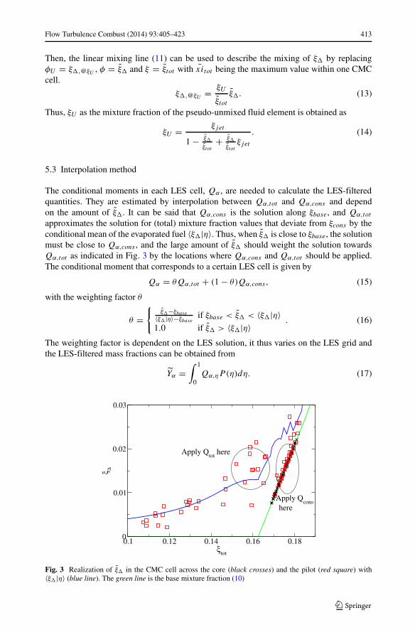
5.3 Interpolation method

The conditional moments in each LES cell, Qα , are needed to calculate the LES-filteredquantities. They are estimated by interpolation between Qα,tot and Qα,cons and dependon the amount of ξ�. It can be said that Qα,cons is the solution along ξbase, and Qα,tot

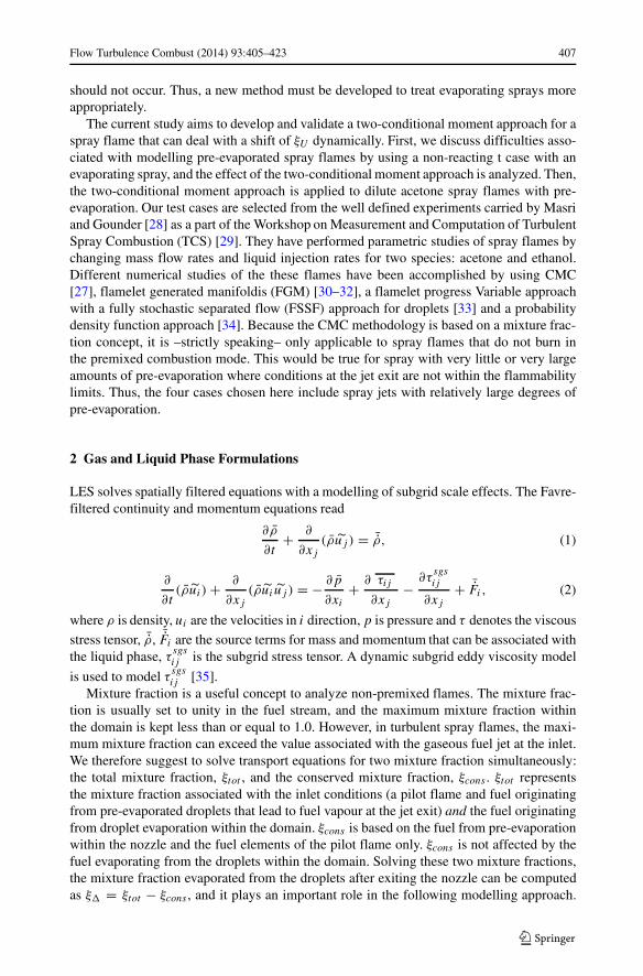
approximates the solution for (total) mixture fraction values that deviate from ξcons by theconditional mean of the evaporated fuel 〈ξ�|η〉. Thus, when ξ� is close to ξbase, the solutionmust be close to Qα,cons , and the large amount of ξ� should weight the solution towardsQα,tot as indicated in Fig. 3 by the locations where Qα,cons and Qα,tot should be applied.The conditional moment that corresponds to a certain LES cell is given by

Qα = θQα,tot + (1 − θ)Qα,cons, (15)

with the weighting factor θ

θ ={

ξ�−ξbase〈ξ�|η〉−ξbaseif ξbase < ξ� < 〈ξ�|η〉

1.0 if ξ� > 〈ξ�|η〉. (16)

The weighting factor is dependent on the LES solution, it thus varies on the LES grid andthe LES-filtered mass fractions can be obtained from

˜Yα =∫ 1

0Qα,ηP (η)dη. (17)

0.1 0.12 0.14 0.16 0.18ξ

tot

0

0.01

0.02

0.03

ξ Δ

Apply Qtot

here

Apply Qcons

here

Fig. 3 Realization of ξ� in the CMC cell across the core (black crosses) and the pilot (red square) with〈ξ�|η〉 (blue line). The green line is the base mixture fraction (10)


5.4 Bounded β-function

A β-function is often utilized to construct the PDF of the mixing field and used to computethe LES-filtered quantities by Eq. 17. However, the current study requires a modification tothe boundary of the β-function due to the dynamic change of ξU . Thus, the bounded β-PDFis implemented as in [40]

P (η) = f (η;p, q, ξL, ξU ) = 1

B(p, q)

(η − ξL)p−1(ξU − η)q−1

(ξU − ξL)p+q−1, (18)

where ξL and ξU are the lower and upper limit of the PDF, and p and q are shape parametersconstructed as

p = ξtot − ξL

ξU − ξL

[

(ξtot − ξL)(ξU − ξtot )

˜

ξ ′′2tot− 1

]

, (19)

q = ξU − ξtot

ξU − ξL

[

(ξtot − ξL)(ξU − ξtot )

˜ξ ′′2tot− 1

]

, (20)

where ˜

ξ ′′2tot is the mixture fraction variance modelled as [36]

˜

ξ ′′2tot = Cξ�2

(

∂ξtot

∂xi

∂ξtot

∂xi

)

, (21)

Cξ is a coefficient set to 0.1, and � is the LES cell size. In this study, ξL is always setto 0.0. Currently, P (η) is assumed to be based on ξtot instead of ξcons by considering twolimiting cases of θ in Eq. 15. Firstly, if θ = 1.0, Qα,η is only based on Qα,η,tot , and ξtot isan appropriate choice to obtain P (η). Secondly, if θ = 0.0, Qα,η is only based on Qα,η,cons ,and the P (η) should be rather based on ξcons . However, when θ = 0.0, ξ� = 0 as in Eq. 16so that ξtot = ξcons , and ξtot would be a good choice for P (η). Since P (η) can be correctlymodelled by ξtot in these two limiting cases, an intermediate solution is assumed to followP (η) based on ξtot .

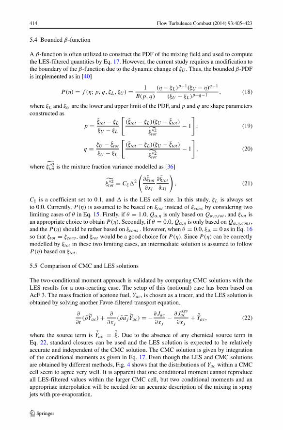
5.5 Comparison of CMC and LES solutions

The two-conditional moment approach is validated by comparing CMC solutions with theLES results for a non-reacting case. The setup of this (notional) case has been based onAcF 3. The mass fraction of acetone fuel, Yac, is chosen as a tracer, and the LES solution isobtained by solving another Favre-filtered transport equation,

∂

∂t(ρ˜Yac)+ ∂

∂xj(ρuj˜Yac) = −∂Jac

∂xj− ∂J

sgsac

∂xj+ ¯Yac, (22)

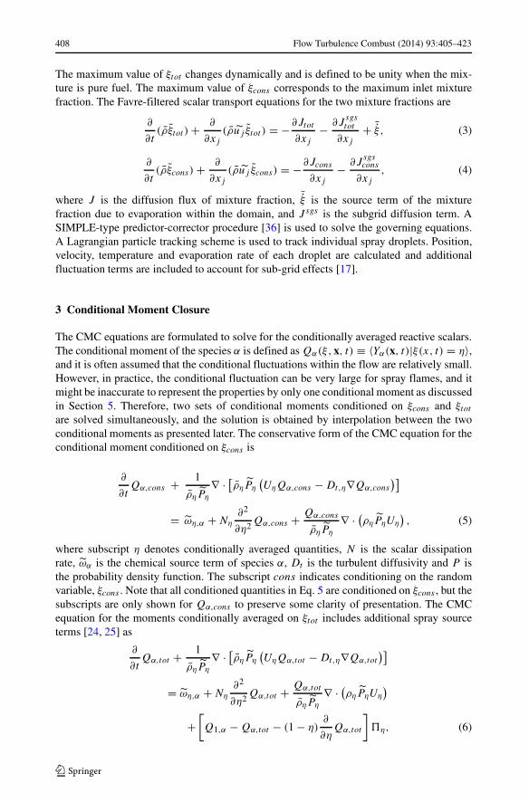
where the source term is ¯Yac = ¯ξ . Due to the absence of any chemical source term inEq. 22, standard closures can be used and the LES solution is expected to be relativelyaccurate and independent of the CMC solution. The CMC solution is given by integrationof the conditional moments as given in Eq. 17. Even though the LES and CMC solutionsare obtained by different methods, Fig. 4 shows that the distributions of Yac within a CMCcell seem to agree very well. It is apparent that one conditional moment cannot reproduceall LES-filtered values within the larger CMC cell, but two conditional moments and anappropriate interpolation will be needed for an accurate description of the mixing in sprayjets with pre-evaporation.


0.1 0.12 0.14 0.16 0.18ξ

tot

0

0.05

0.1

0.15

0.2

Yac

LESCMCQ

totQ

cons

Fig. 4 LES realization of Yac (black plus symbol) and integrated CMC solution (red X symbol) superposedon profiles of Qac,tot (green line) and Qac,cons (blue line)

6 Results and Discussion

The two-conditional moment approach is analyzed and validated in Section 5 for a non-reacting numerical test case by comparisons of acetone mass fractions. In this section,the two-conditional moment approach is tested for the spray flame cases as described inSection 4, and conditional moment profiles, unconditional moments and spray statistics arediscussed.

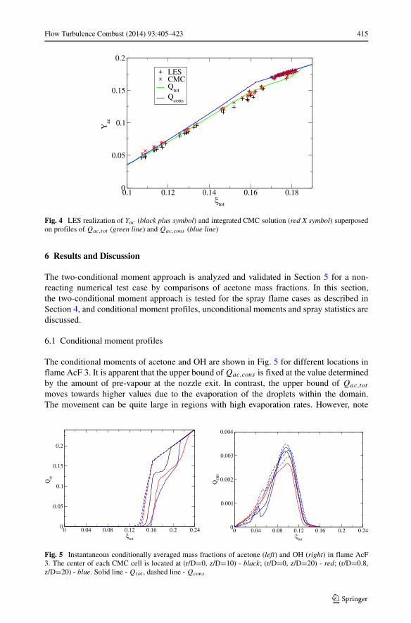
6.1 Conditional moment profiles

The conditional moments of acetone and OH are shown in Fig. 5 for different locations inflame AcF 3. It is apparent that the upper bound of Qac,cons is fixed at the value determinedby the amount of pre-vapour at the nozzle exit. In contrast, the upper bound of Qac,tot

moves towards higher values due to the evaporation of the droplets within the domain.The movement can be quite large in regions with high evaporation rates. However, note

0 0.04 0.08 0.12 0.16 0.2 0.24ξ

tot

0

0.05

0.1

0.15

0.2

Qac

0 0.04 0.08 0.12 0.16 0.2 0.24ξ

tot

0

0.001

0.002

0.003

0.004

QO

H

Fig. 5 Instantaneous conditionally averaged mass fractions of acetone (left) and OH (right) in flame AcF3. The center of each CMC cell is located at (r/D=0, z/D=10) - black; (r/D=0, z/D=20) - red; (r/D=0.8,z/D=20) - blue. Solid line - Qtot , dashed line - Qcons


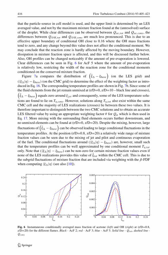
that the particle-source in cell model is used, and the upper limit is determined by an LESaveraged value, and not by the maximum mixture fraction found at the (unresolved) surfaceof the droplet. While clear differences can be observed between Qac,tot and Qac,cons , thedifferences between QOH,tot and QOH,cons are much less pronounced. This is due to aneffective upper boundary of conditional OH close to 0.16 where the OH mass fractionstend to zero, and any change beyond this value does not affect the conditional moment. Wemay conclude that the reaction zone is hardly affected by the moving boundary. However,dissipation in mixture fraction space is affected, and this will be discussed further below.Also, OH profiles can be changed noticeably if the amount of pre-evaporation is lowered.Clear differences can be seen in Fig. 6 for AcF 5 where the amount of pre-evaporationis relatively low, restricting the width of the reaction zone for the conditional momentsconditioned on the conserved mixture fraction.

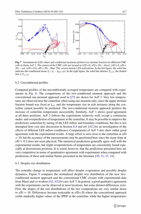
Figure 7a compares the distribution of(

ξ� − ξbase

)

(on the LES grid) and

(〈ξ�|η〉 − ξbase) (on the CMC grid) to determine the effect of the weighting factor as intro-duced in Eq. 16. The corresponding temperature profiles are shown in Fig. 7b. Since some ofthe fluid elements from the jet remain unmixed at (r/D=0, z/D=10 – black line and crosses),(

ξ� − ξbase

)

equals zero around ξjet and consequently, some of the LES temperature solu-

tions are found to lie on Tη,cons . However, solutions along Tη,tot also exist within the sameCMC cell and the majority of LES realizations (crosses) lie between these two values. It istherefore important to distinguish between the two CMC solutions and to obtain an accurateLES filtered value by using an appropriate weighting factor θ for Qα which is then used inEq. 17. More mixing with the surrounding fluid elements occurs further downstream, andno unmixed elements can be found at (r/D=0, z/D=20). Despite the mixing, however, large

fluctuations of(

ξ� − ξbase

)

can be observed leading to large conditional fluctuations in the

temperature profiles. At the position (r/D=0.8, z/D=20) a relatively wide range of mixturefraction values can be seen due to the mixing of jet and pilot and continuous evaporationof the fuel. The conditional fluctuations around (〈ξ�|η〉 − ξbase) are, however, small suchthat the temperature profiles can be well approximated by one conditional moment Tη,totonly. Note that (〈ξ�|η〉 − ξbase) can be non-zero for certain mixture fraction values even ifnone of the LES realizations provides this value of ξtot within the CMC cell. This is due tothe subgrid fluctuations of mixture fraction that are included via weighting with the β-FDFwhen computing 〈ξ�|η〉 (see also [10]).

0 0.04 0.08 0.12 0.16 0.2 0.24ξ

tot

0

0.04

0.08

0.12

0.16

0.2

0.24

Qac

0 0.04 0.08 0.12 0.16 0.2 0.24ξ

tot

0

0.001

0.002

0.003

0.004

0.005

QO

H

Fig. 6 Instantaneous conditionally averaged mass fraction of acetone (left) and OH (right) at (r/D=0.8,z/D=20) for the different flames. Black - AcF 2; red - AcF 3; blue - AcF 5. Solid line - Qtot , dashed line -Qcons


0.08 0.1 0.12 0.14 0.16 0.18 0.2 0.22 0.24ξ

tot

0

0.01

0.02

0.03

0.04

0.05

ξ Δ− ξ ba

se

0.08 0.1 0.12 0.14 0.16 0.18 0.2 0.22 0.24ξ

tot

500

1000

1500

2000

Tem

pera

ture

(K

)

Fig. 7 Instantaneous LES values and conditional moments plotted over mixture fraction for different CMCcells in flame AcF 3. The centers of the CMC cells are located at (r/D=0, z/D=10) – black; (r/D=0, z/D=20) – red; (r/D=0.8, z/D=20) – blue. The crosses denote LES realizations. In the left figure, the solid lineindicates the conditional mean 〈ξ | η〉 − ξbase(η). In the right figure, the solid line denotes Tη,tot , the dashedline is Tη,cons

6.2 Unconditional profiles

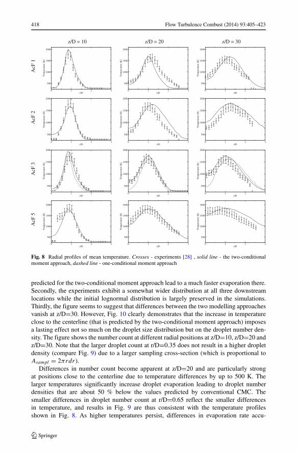
Computed profiles of the unconditionally averaged temperature are compared with exper-iments in Fig. 8. The comparisons of the two-conditional moment approach and theconventional one-moment approach used in [27] are shown for AcF 3. Very low tempera-tures are observed near the centerline when using one moment only, since the upper mixturefraction bound was fixed at ξjet and the temperature rise in rich mixtures along the cen-terline cannot possibly be predicted. The two-conditional moment approach predicts theincrease of centerline temperature successfully. Similarly, AcF 1 shows good agreementat all three positions. AcF 2 follows the experiments relatively well, except a continuousunder- and overprediction of temperature at the centerline. It may be possible to improve thepredictions somewhat by tuning of the LES inflow and boundary conditions, but this is notattempted here (see also discussion in Section 6.4 and ref. [41] for an investigation of theeffects of different LES inflow conditions). Computations of AcF 5 also show rather goodagreement with the experimental results. A large offset is seen close to the centerline at z/D= 10, but the accuracy of the measurements may be questioned here since the steep slope atr/D ≈ 0.2 does not seem physical. The numerical predictions generally agree well with theexperimental results, but slight overpredictions of temperature are consistently found espe-cially at downstream positions. It is noted, however, that the predictions presented here arevery competitive in terms of quantitative agreement with experiments when compared withpredictions of these and similar flames presented in the literature [30, 31, 33, 34].

6.3 Droplet size distribution

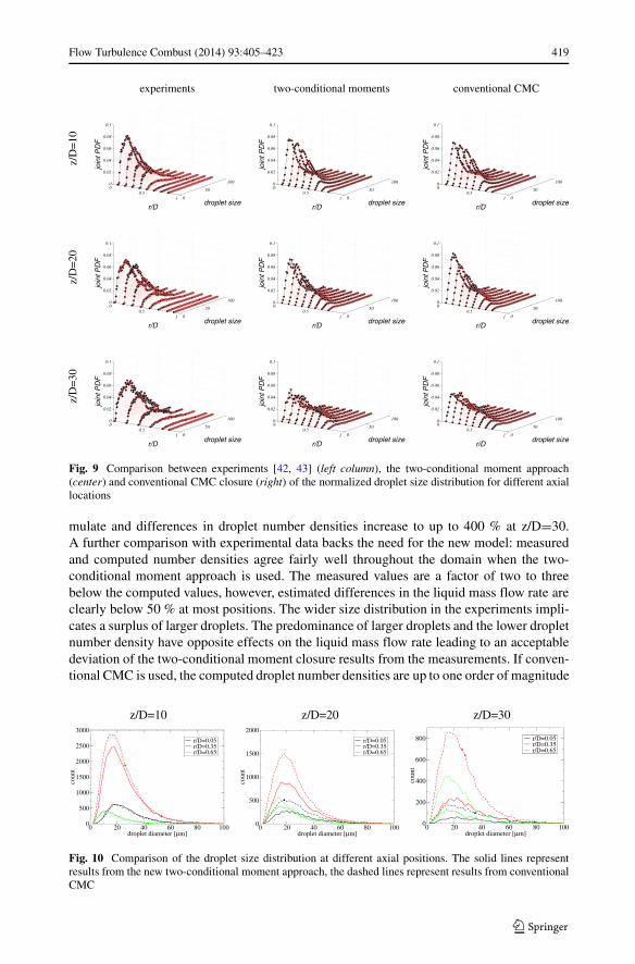
The noteable change in temperature will affect droplet evaporation and possibly dropletdynamics. Figure 9 compares the normalized droplet size distribution of the new two-conditional moment approach and the conventional CMC closure with experimental datafrom Masri and co-workers [42, 43] for case AcF 3. In general, a good qualitative agreementwith the experiments can be observed at most locations, but some distinct differences exist.First, the shapes of the size distributions of the two computations are very similar downto z/D = 10. Differences become noticeable at z/D=20 where the conventional approachyields markedly higher values of the JPDF at the centerline while the higher temperatures


0 1 2 3r/D

500

1000

1500

2000

Tem

pera

ture

(K

)

0 1 2 3r/D

500

1000

1500

2000

Tem

pera

ture

(K

)

0 1 2 3r/D

500

1000

1500

2000

Tem

pera

ture

(K

)

0 1 2 3r/D

500

1000

1500

2000

Tem

pera

ture

(K

)

0 1 2 3r/D

500

1000

1500

2000

Tem

pera

ture

(K

)

0 1 2 3r/D

500

1000

1500

2000

Tem

pera

ture

(K

)

0 1 2 3r/D

500

1000

1500

2000

Tem

pera

ture

(K

)

0 1 2 3r/D

500

1000

1500

2000

Tem

pera

ture

(K

)

0 1 2 3r/D

500

1000

1500

2000

Tem

pera

ture

(K

)

0 1 2 3r/D

500

1000

1500

2000

Tem

pera

ture

(K

)

0 1 2 3r/D

500

1000

1500

2000

Tem

pera

ture

(K

)

0 1 2 3r/D

500

1000

1500

2000

Tem

pera

ture

(K

)

Fig. 8 Radial profiles of mean temperature. Crosses - experiments [28] , solid line - the two-conditionalmoment approach, dashed line - one-conditional moment approach

predicted for the two-conditional moment approach lead to a much faster evaporation there.Secondly, the experiments exhibit a somewhat wider distribution at all three downstreamlocations while the initial lognormal distribution is largely preserved in the simulations.Thirdly, the figure seems to suggest that differences between the two modelling approachesvanish at z/D=30. However, Fig. 10 clearly demonstrates that the increase in temperatureclose to the centerline (that is predicted by the two-conditional moment approach) imposesa lasting effect not so much on the droplet size distribution but on the droplet number den-sity. The figure shows the number count at different radial positions at z/D=10, z/D=20 andz/D=30. Note that the larger droplet count at r/D=0.35 does not result in a higher dropletdensity (compare Fig. 9) due to a larger sampling cross-section (which is proportional toAsampl = 2πrdr).

Differences in number count become apparent at z/D=20 and are particularly strongat positions close to the centerline due to temperature differences by up to 500 K. Thelarger temperatures significantly increase droplet evaporation leading to droplet numberdensities that are about 50 % below the values predicted by conventional CMC. Thesmaller differences in droplet number count at r/D=0.65 reflect the smaller differencesin temperature, and results in Fig. 9 are thus consistent with the temperature profilesshown in Fig. 8. As higher temperatures persist, differences in evaporation rate accu-


00.5

1 0

50

1000

0.02

0.04

0.06

0.08

0.1

droplet sizer/D

join

t PD

F

00.5

1 0

50

1000

0.02

0.04

0.06

0.08

0.1

droplet sizer/D

join

t PD

F

00.5

1 0

50

1000

0.02

0.04

0.06

0.08

0.1

droplet sizer/D

join

t PD

F

00.5

1 0

50

1000

0.02

0.04

0.06

0.08

0.1

droplet sizer/D

join

t PD

F

00.5

1 0

50

1000

0.02

0.04

0.06

0.08

0.1

droplet sizer/D

join

t PD

F

00.5

1 0

50

1000

0.02

0.04

0.06

0.08

0.1

droplet sizer/D

join

t PD

F0

0.51 0

50

1000

0.02

0.04

0.06

0.08

0.1

droplet sizer/D

join

t PD

F

00.5

1 0

50

1000

0.02

0.04

0.06

0.08

0.1

droplet sizer/D

join

t PD

F

00.5

1 0

50

1000

0.02

0.04

0.06

0.08

0.1

droplet sizer/D

join

t PD

F

Fig. 9 Comparison between experiments [42, 43] (left column), the two-conditional moment approach(center) and conventional CMC closure (right) of the normalized droplet size distribution for different axiallocations

mulate and differences in droplet number densities increase to up to 400 % at z/D=30.A further comparison with experimental data backs the need for the new model: measuredand computed number densities agree fairly well throughout the domain when the two-conditional moment approach is used. The measured values are a factor of two to threebelow the computed values, however, estimated differences in the liquid mass flow rate areclearly below 50 % at most positions. The wider size distribution in the experiments impli-cates a surplus of larger droplets. The predominance of larger droplets and the lower dropletnumber density have opposite effects on the liquid mass flow rate leading to an acceptabledeviation of the two-conditional moment closure results from the measurements. If conven-tional CMC is used, the computed droplet number densities are up to one order of magnitude

0 20 40 60 80 100droplet diameter [μm]

0

500

1000

1500

2000

2500

3000

coun

t

r/D=0.05r/D=0.35r/D=0.65


0

500

1000

1500

2000

coun

t

r/D=0.05r/D=0.35r/D=0.65


0

200

400

600

800

coun

t

r/D=0.05r/D=0.35r/D=0.65

Fig. 10 Comparison of the droplet size distribution at different axial positions. The solid lines representresults from the new two-conditional moment approach, the dashed lines represent results from conventionalCMC


above the measured values at z/D=30 and estimates of the predicted liquid mass flow ratesare up to three times above the experimental values.

6.4 Spray velocity statistics

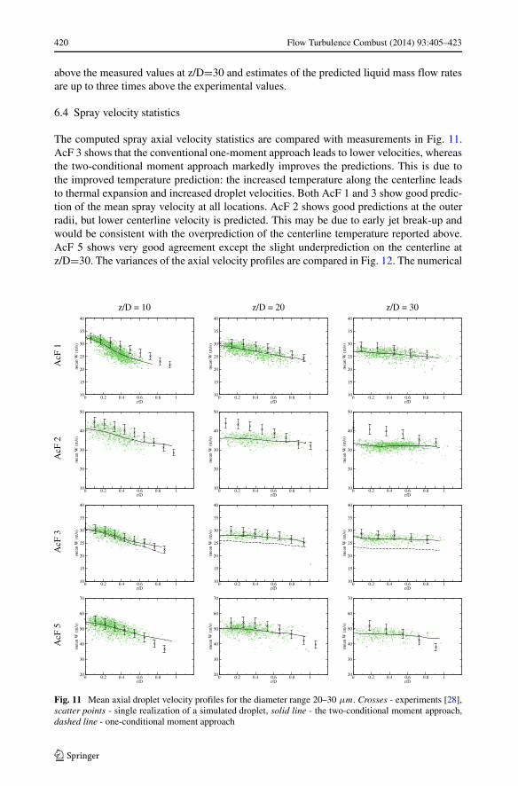
The computed spray axial velocity statistics are compared with measurements in Fig. 11.AcF 3 shows that the conventional one-moment approach leads to lower velocities, whereasthe two-conditional moment approach markedly improves the predictions. This is due tothe improved temperature prediction: the increased temperature along the centerline leadsto thermal expansion and increased droplet velocities. Both AcF 1 and 3 show good predic-tion of the mean spray velocity at all locations. AcF 2 shows good predictions at the outerradii, but lower centerline velocity is predicted. This may be due to early jet break-up andwould be consistent with the overprediction of the centerline temperature reported above.AcF 5 shows very good agreement except the slight underprediction on the centerline atz/D=30. The variances of the axial velocity profiles are compared in Fig. 12. The numerical

Fig. 11 Mean axial droplet velocity profiles for the diameter range 20–30 μm. Crosses - experiments [28],scatter points - single realization of a simulated droplet, solid line - the two-conditional moment approach,dashed line - one-conditional moment approach


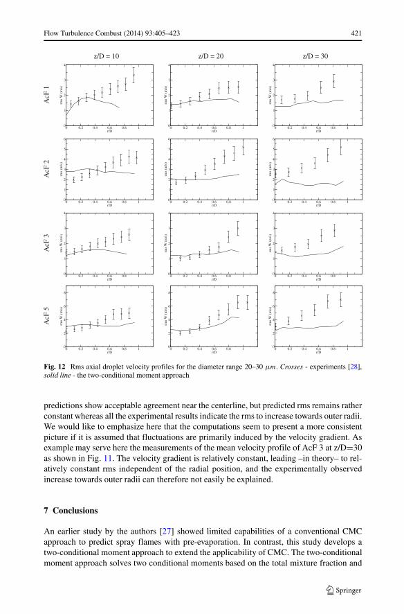
Fig. 12 Rms axial droplet velocity profiles for the diameter range 20–30 μm. Crosses - experiments [28],solid line - the two-conditional moment approach

predictions show acceptable agreement near the centerline, but predicted rms remains ratherconstant whereas all the experimental results indicate the rms to increase towards outer radii.We would like to emphasize here that the computations seem to present a more consistentpicture if it is assumed that fluctuations are primarily induced by the velocity gradient. Asexample may serve here the measurements of the mean velocity profile of AcF 3 at z/D=30as shown in Fig. 11. The velocity gradient is relatively constant, leading –in theory– to rel-atively constant rms independent of the radial position, and the experimentally observedincrease towards outer radii can therefore not easily be explained.

7 Conclusions

An earlier study by the authors [27] showed limited capabilities of a conventional CMCapproach to predict spray flames with pre-evaporation. In contrast, this study develops atwo-conditional moment approach to extend the applicability of CMC. The two-conditionalmoment approach solves two conditional moments based on the total mixture fraction and


the conserved mixture fraction to account for the shift of the upper limit of mixture fractiondue to the evaporation process. A new method to select the upper boundary is also proposed,and the two-conditional moment is tested and validated using non-reacting test case. Then,we validated the methodology by its application to a wide range of flames with differentdegrees of pre-evaporation (and Reynolds numbers). Four cases have been selected from theseries of acetone flame experiments [28]. The conditional moment profiles clearly demon-strate the effects of the two-conditional moment approach. The conditional moment basedon ξtot becomes very important when non-reacting and reacting solutions co-exist withinone CMC cell. Using the correct weighting between the two moments leads to significantimprovements of the predicted radial temperature profiles, particularly near the centerline.It is also shown that the new model is robust enough to predict a flame series with varyingdegrees of pre-evaporation as long as the equivalence ratio of the fuel vapour exiting the jetdoes not allow for a flame burning largely in the premixed mode. Predictions of the spraymean velocity have also been improved. The mean velocity profiles show good agreement,but a slight underestimation is consistently found downstream. The predictions of the axialvelocity rms are acceptable along the centerline, but the experimental trend of an increaseof the rms at the outer radii is not captured.

Acknowledgements The authors would like to acknowledge the funding support by DFG (grant no.KR3684/1-2) and the computational resources provided by HLRS. We would also like to thank Profs. A.Masri and W. P. Jones for providing the experimental data sets and the original CFD routines, respectively.

References

1. Jenny, P., Roekaerts, D., Beishuizen, N.: Modeling of turbulent dilute spray combustion. Prog. EnergyCombust. Sci. 38(6), 846–887 (2012)

2. Pierce, C.D., Moin, P.: Progress-variable approach for large-eddy simulation of non-premixed turbulentcombustion. J. Fluid Mech. 504, 73–97 (2004)

3. Ihme, M., Pitsch, H.: Prediction of extinction and reignition in nonpremixed turbulent flames usinga flamelet/progress variable model: 2. application in les of sandia flames D and E. Combust. Flame155(1–2), 90–107 (2008)

4. Vreman, A., Albrecht, B., van Oijen, J., de Goey, L., Bastiaans, R.: Premixed and nonpremixed generatedmanifolds in large-eddy simulation of sandia flame D and F. Combust. Flame 153(3), 394–416 (2008)

5. Olbricht, C., Stein, O.T., Janicka, J., van Oijen, J.A., Wysocki, S., Kempf, A.M.: LES of lifted flames ina gas turbine model combustor using top-hat filtered PFGM chemistry. Fuel 96(1), 100–107 (2012)

6. Jaberi, F., Colucci, P., James, S., Givi, P., Pope, S.: Filtered mass density function for large-eddysimulation of turbulent reacting flows. J. Fluid Mech. 401, 85–121 (1999)

7. Menon, S., Patel, N.: Subgrid modeling for simulation of spray combustion in large-scale combustors.AIAA J. 44, 709–723 (2006)

8. Prasad, V.N., Masri, A.R., Navarro-Martinez, S., Luo, K.H.: Investigation of auto-ignition in turbulentmethanol spray flames using Large Eddy Simulation. Comb. Flame 160(12), 2941–2954 (2013)

9. Ge, Y., Cleary, M., Klimenko, A.: A comparative study of Sandia flame series (D-F) using sparse-Lagrangian MMC modelling. Proc. Comb. Inst. 34(1), 1325–1332 (2013)

10. Navarro-Martinez, S., Kronenburg, A., Mare, F.D.: Conditional moment closure for large eddy simula-tions. Flow Turb. Combust. 75, 245–274 (2005)

11. Garmory, A., Mastorakos, E.: Capturing localised extinction in Sandia flame F with LES-CMC. Proc.Comb. Inst. 33(1), 1673–1680 (2011)

12. Navarro-Martinez, S., Kronenburg, A.: LES-CMC simulations of a turbulent bluff-body flame. Proc.Combust. Inst. 31, 1721–1728 (2007)

13. Navarro-Martinez, S., Kronenburg, A.: LES-CMC simulations of a turbulent a lifted methane flame.Proc. Combust. Inst. 32, 1509–1516 (2009)

14. Patwardhan, S., De, S., Lakshmisha, K., Raghunandan, B.: CMC simulations of lifted turbulent jet flamein a vitiated coflow. Proc. Comb. Inst. 32(2), 1705–1712 (2009)


15. Navarro-Martinez, S., Kronenburg, A.: Flame stabilization mechanisms in lifted flames. Flow Turb.Combust. 87, 377–406 (2011)

16. Stankovic, I., Mastorakos, E., Merci, B.: LES-CMC simulations of different auto-ignition regimes ofhydrogen in a hot turbulent air co-flow. Flow Turb. Combust. 90(3), 583–604 (2013)

17. Bini, M., Jones, W.P.: Large eddy simulation of an evaporating acetone spray. Int. J. Heat Fluid Flow 30,471–480 (2009)

18. De, S., Lakshmisha, K., Bilger, R.W.: Modeling of nonreacting and reacting turbulent spray jets using afully stochastic separated flow approach. Comb. Flame 158(10), 1992–2008 (2011)

19. Wright, Y., Paola, G.D., Boulouchos, K., Mastorakos, E.: Simulations of spray autoignition and flameestablishment with two-dimensional CMC. Combust. Flame 143(4), 402–419 (2005)

20. Wright, Y., Margari, O.-N., Boulouchos, K., De Paola, G., Mastorakos, E.: Experiments and simulationsof n-heptane spray auto-ignition in a closed combustion chamber at diesel engine conditions. Flow Turb.Combust. 84, 49–78 (2010)

21. Bottone, F., Kronenburg, A., Gosman, D., Marquis, A.: The numerical simulation of diesel spraycombustion with LES-CMC. Flow Turb. Combust. 89(4), 651–673 (2012)

22. Kim, W.T., Huh, K.Y.: Numerical simulation of spray autoignition by the first-order conditional momentclosure model. Proc. Comb. Inst. 29, 569–576 (2002)

23. Rogerson, J., Kent, J., Bilger, R.: Conditional moment closure in a bagasse-fired boiler. Proc. Combust.Inst. 31(2), 2805–2811 (2007)

24. Mortensen, M., Bilger, R.: Derivation of the conditional moment closure equations for spray combustion.Combust. Flame 156(1), 62–72 (2009)

25. Borghesi, G., Mastorakos, E., Devaud, C.B., Bilger, R.W.: Modeling evaporation effects in conditionalmoment closure for spray autoignition. Combust. Theo. Model 15(5), 725–752 (2011)

26. Tyliszczak, A., Cavaliere, D., Mastorakos, E.: LES/CMC of blow-off in a liquid fueled swirl burner.Flow Turbul. Combust. 92(1–2), 237–267 (2014). doi:10.1007/s10494-013-9477-5

27. Ukai, S., Kronenburg, A., Stein, O.T.: LES-CMC of a dilute acetone spray flame. Proc. Combust. Inst.34(1), 1643–1650 (2013)

28. Masri, A.R., Gounder, J.D.: Turbulent spray flames of acetone and ethanol approaching extinction.Combust. Sci. Techn. 182(4), 702–715 (2010)

29. Merci, B., Roekaerts, D., Sadiki, A.: Experiments and numerical simulations of diluted spray turbulentcombustion. Springer (2011)

30. Chrigui, M., Gounder, J., Sadiki, A., Masri, A.R., Janicka, J.: Partially premixed reacting acetone sprayusing LES and FGM tabulated chemistry. Combust. Flame 159(8), 2718–2741 (2012)

31. Chrigui, M., Gounder, J., Sadiki, A., Janicka, J., Masri, A.: Acetone droplet behavior in reacting and nonreacting turbulent flow. Flow. Turb. Comb. 90(2), 419–447 (2013)

32. Chrigui, M., Masri, A.R., Sadiki, A., Janicka, J.: Large eddy simulation of a polydisperse ethanol sprayflame. Flow. Turb. Comb. 90(4), 813–832 (2013)

33. De, S., Kim, S.H.: Large eddy simulation of dilute reacting sprays: droplet evaporation and scalar mixing.Combust. Flame 160(10), 2048–2066 (2013)

34. Heye, C., Raman, V., Masri, A.R.: LES/probability density function approach for the simulation of anethanol spray flame. Proc. Comb. Inst. 34(1), 1633–1641 (2013)

35. Germano, M., Piomelli, U., Moin, P., Cabot, W.H., dynamic subgrid-scale eddy viscosity model: Phys.Fluids A 3(7), 1760–1765 (1991)

36. Branley, N., Jones, W.P.: Large eddy simulation of a turbulent non-premixed flame. Combust. Flame127, 1914–1934 (2001)

37. Barlow, R., Karpetis, A., Frank, J., Chen, J.-Y.: Scalar profiles and NO formation in laminar opposed-flow partially premixed methane/air flames. Combust. Flame 127(3), 2102–2118 (2001)

38. Klein, M., Sadiki, A., Janicka, J.: A digital filter based generation of inflow data for spatially developingdirect numerical or large eddy simulations. J. Comput. Phys. 186(2), 652–665 (2003)

39. Chong, C., Hochgreb, S.: Measurements of laminar flame speeds of acetone/methane/air mixtures.Combust. Flame 158(8), 490–500 (2011)

40. Ge, H.-W., Gutheil, E.: Probability density function (pdf) simulation of turbulent spray flows. Atomiza-tion and Sprays 16(5), 531–542 (2006)

41. Dietzel, D., Messig, D., Piscaglia, F., Montorfano, A., Olenik, G., Stein, O., Kronenburg, A., Onorati,A., Hasse, C.: Evaluation of sclae resolving turbulence generation methods for large eddy simulation ofturbulent flows. Comp. Fluids 93, 116–128 (2014)

42. Gounder, J., Kourmatzis, A., Masri, A.: Turbulent piloted dilute spray flames: Flow fields and dropletdynamics. Combust. Flame 159, 3372–3397 (2012)

43. Kourmatzis, A., O’Loughlin, W., Masri, A.: Effects of turbulence, evaporation and heat release on thedispersion of droplets in dilute spray jets and flames. Flow Turbul. Combust. 91, 405–427 (2013)

http://dx.doi.org/10.1007/s10494-013-9477-5

Documents

Simulation of Dilute Acetone Spray Flames with LES-CMC Using Two Conditional Moments