Embed Size (px)
Citation preview

Simulation of Continuously Variable Transmission
Chain Drives with Involute Inter-element Contact Surfaces
by
THOMAS HEENAN BRADLEY B.S. (University of California, Davis) 2000
THESIS
Submitted in partial satisfaction of the requirements for the degree of
MASTER OF SCIENCE
in
Mechanical Engineering
in the
OFFICE OF GRADUATE STUDIES
of the
UNIVERSITY OF CALIFORNIA
DAVIS
Approved:
Committee in Charge
2003
i

Copyright by
THOMAS HEENAN BRADLEY
2003
ii

T. H. Bradley
ABSTRACT
Static and dynamic simulations of a continuously variable transmission (CVT)
chain and pulley system are developed in the MATLAB environment to determine the
effect of a power transmissions chain with involute inter-element contact surfaces on
polygonal action in CVT systems. The static simulations consist of a geometric model of
the kinematics of the CVT chain and are used as a design tool for investigating tradeoffs
in contact surface design. The dynamic simulations consists of a system of lumped
parameter rigid body models that represent the elements of the CVT chain and the pulleys
of the CVT. The chain elements are joined using compliance and damping elements.
The chain system interacts with the pulleys through Hertzian contact compliances and a
two-dimensional explicit slip-stick friction model. The characteristics of the chain and
pulley system are chosen to emulate a prototype 2L CVT chain manufactured by Gear
Chain Industrial. The simulated static and dynamic behavior of this CVT chain exhibits
reduced polygonal action when compared to a CVT chain with pinned-joint inter-element
contacts.
iii

T. H. Bradley
ACKNOWLEDGEMENTS
This research has been supported in part by the United States Department of
Energy Graduate Automotive Engineering Education Fellowship, Koyo Seiko
Corporation Ltd. and Gear Chain Industrial B. V. Of course, this project would have
been impossible without the support of Dr. Andy Frank and the students and staff of the
University of California, Davis Hybrid Electric Vehicle Research Center. I have been
privileged to work among this group of talented and dedicated individuals.
iv
T. H. Bradley
TABLE OF CONTENTS
LIST OF FIGURES .......................................................................................................... vii LIST OF TABLES........................................................................................................... viii LIST OF SYMBOLS ......................................................................................................... ix INTRODUCTION .............................................................................................................. 1
Continuously Variable Transmission Drive Technologies ............................................. 1
GCI CVT Chain Design Description .............................................................................. 2
Polygonal Action ............................................................................................................ 3
Objectives ....................................................................................................................... 5
STATIC MODELS OF AN INVOLUTE CVT CHAIN .................................................... 7 Continuous Static Chain Model ...................................................................................... 7
Involute Contact Surface Derivation .......................................................................... 7
Limitations of the Continuous Static Chain Model .................................................... 9
Discrete Static Chain Model ......................................................................................... 10
Formulation of Equations ......................................................................................... 11
Solver ........................................................................................................................ 12
Results....................................................................................................................... 13
DYNAMIC MODEL OF AN INVOLUTE CVT CHAIN ............................................... 21 Constitutive Component Models .................................................................................. 21
Chain Model Description and Validation ................................................................. 21
Contact Model Description and Validation .............................................................. 29
Friction Model Description and Validation .............................................................. 35
Modeled Link and Pulley Characteristics ................................................................. 40
Mathematical Formulation............................................................................................ 41
Formulation of Equations ......................................................................................... 41
Solver ........................................................................................................................ 42
v

T. H. Bradley
Simulation Evaluation Methods.................................................................................... 42
Results and Discussion ................................................................................................. 44
CONCLUSIONS AND RECOMMENDATIONS ........................................................... 51 REFERENCES ................................................................................................................. 53 APPENDIX 1 – Discrete Static CVT Chain Model: MATLAB M-files.......................... 56
inv.m ............................................................................................................................. 56
involute_fxn6.m............................................................................................................ 58
APPENDIX 2 – Dynamic CVT Chain Model: MATLAB M-files .................................. 63 chain_init_v13f.m ......................................................................................................... 63
chain_ode_v13f.m......................................................................................................... 69
APPENDIX 3 – Linear Elastic Link Compliance Calculation: MATLAB M-file........... 76 link_comp.m ................................................................................................................. 76
vi

T. H. Bradley
LIST OF FIGURES
Figure 1. Reeves-type Continuously Variable Transmission 1 Figure 2. Van Doorne CVT Belt Assembly 1 Figure 3. GCI Chain Assembly [van Rooij 1996] 2 Figure 4. Illustration of Polygonal Action 4 Figure 5. GCI Chain at Pulley Entrance [van Rooij 1996] 5 Figure 6. CVT Chain Entrance Definitions 8 Figure 7. Involute Chain, Line of Action Tangent to Contact Circle [van Rooij 1996] 10 Figure 8. Chain Element Vector and Coordinate Definitions (as in [van Rooij 1996]) 11 Figure 9. Chain Path and Definitions for Involute and Pinned CVT Chains (Vertical axis
is exaggerated for clarity) 14 Figure 10. Pinned Joint CVT Chain, Line of Action Displaced from Tangent Line 14 Figure 11. Y-direction Distance of Impact from Tangent for Involute and Roller CVT
Chains 15 Figure 12. Impact Incidence Angle for Involute and Roller CVT Chains 16 Figure 13. Chain Path for Involute Chains of Different Base Radii 18 Figure 14. Y-direction Distance of Impact from Tangent for Involute Chains of Various
Rb 19 Figure 15. Amplitude of Element no. 5 Oscillation in y_e direction for Involute Chains of
Various Rb 20 Figure 16. X and Y Direction Link Compliance Model 22 Figure 17. Element Definitions and Pin Loading Diagrams 23 Figure 18. Pin Deformation for Joint Type 2, P = 437.5 N 24 Figure 19. Modeled Sources of Inter-Element Compliance 25 Figure 20. Chain Element Natural Period Validation 27 Figure 21. Chain Mode Shapes and CG Locations 28 Figure 22. Pin Compliance Model 30 Figure 23. Chain Pin Compliance Models 31 Figure 24. Frictionless Pin to Pulley Impact Simulation 32 Figure 25. Frictionless Contact Model Validation 34 Figure 26. Friction Law Comparison 36 Figure 27. Chain Link Contact Configuration 37 Figure 28. Slip Stick Oscillator 38 Figure 29. Slip Stick Oscillator Trajectory 39 Figure 30. Chain Element Motion at Pulley Entrance 44 Figure 31. Pinned Contact Chain Span Motion 46 Figure 32. Involute Contact Chain Span Motion 47 Figure 33. Frequency Spectra for Pinned and Involute Contact Chains 48 Figure 34. Secondary Pulley Torque Profile 49
vii

T. H. Bradley
LIST OF TABLES
Table 1. Comparison of Numerical and Analytical Span Vibration Solutions................. 29 Table 2. Contact Model Validation Results...................................................................... 33 Table 3. Rigid Body Contact Model Validation Results .................................................. 34 Table 4. Slip Stick Oscillator Operating Conditions ........................................................ 38 Table 5. Simulation Parameters for Dynamic Model ....................................................... 43
viii

T. H. Bradley
LIST OF SYMBOLS
Symbol Description Units a Diameter of contact patch [m] A Area of load bearing material in chain link [m2]
A_b Position of the upstream inter-element contact when chain is uncurved in the chain element reference frame
[m]
A_bc Position of the upstream pin to pulley contact when chain is uncurved in the chain element reference frame
[m]
β Pulley half-angle [rad] B_b Position of the downstream inter-element contact when chain
is uncurved in the chain element reference frame [m]
d Static mid-span peak to peak displacement in the y_e direction [m/s] δ Contact displacement perpendicular to contact surface [m] dh Distance in the y_e direction between the point tangent to
contact circle and parallel to chain span and the point of pin to pulley impact
[m]
DV Karnopp friction stick velocity [m/s] ε Angular difference between θ and angle between x_b and x_e
for chain elements in pulley contact [rad/sec]
E, E* Young's modulus [Pa] F General contact force [N] Fcomp Compressive pin to pulley contact force [N]
Fdamp Compressive pin to pulley damping force under contact [N]
γ Angular difference between θi and θi+1 for chain elements in pulley contact
[rad/sec]
g Acceleration due to gravity [m/s2]
h Vector of inter element contact forces for dynamic chain system
[N]
i Index of chain elements [-]
I_link Inertia of chain element about its center of gravity [kg m2]
k_lin Translational stiffness of inter-element joint for validation [N/m] k_rot Rotational stiffness of inter-element joint for validation [N/rad] kelastic Elastic pin stiffness in compression [N/m]
khertz Herztian contact stiffness [N/m]
kpin_bending Linear stiffness of pin to bending forces [N/m]
ix

T. H. Bradley
κs Herztian contact stiffness [N/m]
Kspring Translational stiffness of inter-element joint for validation [N/m]
L Approximate length of chain link [m] l Chain span length [m] L Pin length in z_e direction [m] λ Vector of contact forces for dynamic chain system [N] M Mass of chain element [kg] µd Dynamic coefficient of friction [-]
µs Static coefficient of friction [-]
n Mode number [-] nplates Number of link plates per chain element [-]
P Contact force [N] P Chain element momentum [kg m/s]θ Angle from y_e axis for chain pin in contact with the pulley [rad] q State vector for dynamic chain system [-] Qi Position vector for point of pin to pulley contact [m]
θi Angular difference between element and earth coordinate systems
[rad]
R Radius on the pulley of the equilibrium contact circle [m] R Radius of cylindrical body under contact [m] ρ 1-dimensional density of chain span [N/m] Rb Involute base radius [m] S1 Linear distance traveled by the chain span after contact with
pulleys [m]
Τ ι Coordinate transformation matrix from earth to chain element body coordinates
[-]
τ Natural period of oscillation of single chain element [s] tc Period of Hertzian contact [s]
Tcont Analytically derived natural period of oscillation for continuous chain span
[s]
Tnum Numerically derived natural period of oscillation for discrete chain span
[s]
Ttens Tensile force in chain span [N]
υ Poisson's ratio [-] v Chain span linear velocity [m/s] v,V Chain span and chain element velocity [m/s] Vpul Relative velocity of the pulley to the chain element for
lid i [m/s]
x

T. H. Bradley
validation
ω Rotational Speed of the pulley (counter-clockwise +) [rad/sec]x_b Unit vector in the chain element reference frame [-] x_e Unit vector in the earth reference frame [-] xi Displacement along the involute contact surface in the x_b
direction [m]
xoutput Vector of equilibrium states for static simulation [-]
y_b Unit vector in the chain element reference frame [-] y_e Unit vector in the earth reference frame [-] yi Displacement along the involute contact surface in the y_b
direction [m]
z_e Unit vector in the earth reference frame [-]
xi

T. H. Bradley 1
INTRODUCTION
Continuously Variable Transmission Drive Technologies
In automotive applications, continuously variable transmissions (CVTs) are
proven to give significant improvement in vehicle fuel economy over conventional
automatic transmissions because of the higher ratio range, lower speed torque converter
lock-up, and continuously variable engine operation control available in a CVT [Hirano
1991; Hendricks 1993; Kluger 1999]. Presently, most automotive CVTs brought to
production have been of the Reeves type shown in Figure 1, utilizing movable cone
pulleys and a torque transmitting belt or chain [Reeves 1897]. A vast majority of
automotive CVTs have incorporated a Van Doorne CVT push-belt, shown in Figure 2,
because it is an available and proven technology. Automotive application of CVTs, in
general, are limited to compact vehicles because of the low torque capacity and low
power transmission efficiency of Van Doorne CVTs [Brandsma 1999; Abo 2000; Ide
2000].
Figure 1. Reeves-type Continuously Variable Transmission
Figure 2. Van Doorne CVT Belt Assembly
T. H. Bradley 2
Various technologies have been developed that improve on the torque capacity
and power transmission efficiency of the Van Doorne CVT to allow application of CVT
technology to full-sized vehicles. These technologies include toroidal CVTs, hybrid
(aluminum/composite) belt CVTs, and CVT chains [Takahashi 1999; Tanaka 1999; van
Rooij 2002]. CVT chains are perhaps the most promising of these technologies because
of their very high torque capacity, high efficiency and low-cost materials and
manufacturing processes [van Rooij 1991]. Chain CVT as manufactured by LuK, Borg
Warner and others are usually characterized by increased noise and vibration emissions
compared with Van Doorne CVTs because of the discrete nature of the chain drive
[Avramidis 1986; van Rooij 1993; Bradley 2002]. To address these problems, Gear
Chain Industrial B.V. (GCI) has developed a CVT chain that uses involute inter-element
contact surfaces to minimize noise and vibration.
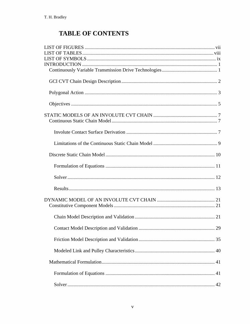
GCI CVT Chain Design Description
The GCI CVT chain is made up of three types of element: links (1), pins (2) and
strips (3). Figure 3 is an illustration of these parts assembled into an interlocking chain.
Figure 3. GCI Chain Assembly [van Rooij 1996]
T. H. Bradley 3
When assembled, the pins are fixed to the leading link and the strips are fixed to
the following link, where the leading link is in the direction of motion. The GCI chain
can use the same conical pulleys that are used for the Van Doorne belt, allowing direct
replacement. Torque is transferred in the CVT by traction between the CVT pulleys and
the pins of the chain. Because the pins are wider than the strips, only the pins contact the
pulley surface and only the pins are subjected to compressive loading from the pulleys.
Unlike the Van Doorne CVT belt, torque is transmitted by tension in the chain. The
tension in the chain causes a line of contact between the pins and the strips of each
element at point C.
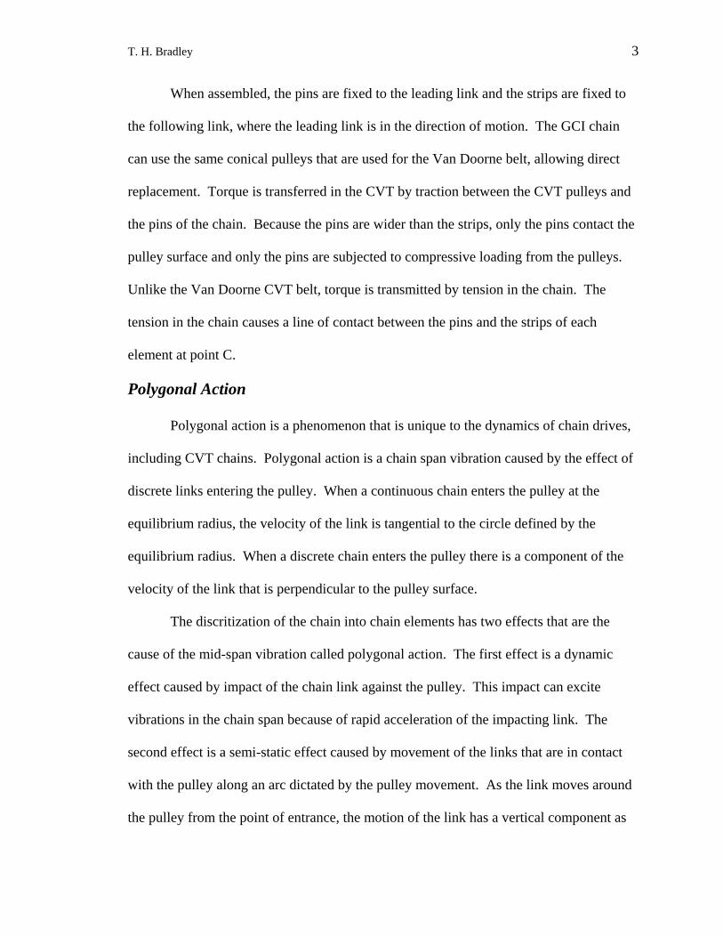
Polygonal Action
Polygonal action is a phenomenon that is unique to the dynamics of chain drives,
including CVT chains. Polygonal action is a chain span vibration caused by the effect of
discrete links entering the pulley. When a continuous chain enters the pulley at the
equilibrium radius, the velocity of the link is tangential to the circle defined by the
equilibrium radius. When a discrete chain enters the pulley there is a component of the
velocity of the link that is perpendicular to the pulley surface.
The discritization of the chain into chain elements has two effects that are the
cause of the mid-span vibration called polygonal action. The first effect is a dynamic
effect caused by impact of the chain link against the pulley. This impact can excite
vibrations in the chain span because of rapid acceleration of the impacting link. The
second effect is a semi-static effect caused by movement of the links that are in contact
with the pulley along an arc dictated by the pulley movement. As the link moves around
the pulley from the point of entrance, the motion of the link has a vertical component as
T. H. Bradley 4
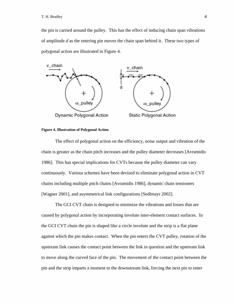
the pin is carried around the pulley. This has the effect of inducing chain span vibrations
of amplitude d as the entering pin moves the chain span behind it. These two types of
polygonal action are illustrated in Figure 4.
Figure 4. Illustration of Polygonal Action
The effect of polygonal action on the efficiency, noise output and vibration of the
chain is greater as the chain pitch increases and the pulley diameter decreases [Avramidis
1986]. This has special implications for CVTs because the pulley diameter can vary
continuously. Various schemes have been devised to eliminate polygonal action in CVT
chains including multiple pitch chains [Avramidis 1986], dynamic chain tensioners
[Wagner 2001], and asymmetrical link configurations [Sedlmayr 2002].
The GCI CVT chain is designed to minimize the vibrations and losses that are
caused by polygonal action by incorporating involute inter-element contact surfaces. In
the GCI CVT chain the pin is shaped like a circle involute and the strip is a flat plane
against which the pin makes contact. When the pin enters the CVT pulley, rotation of the
upstream link causes the contact point between the link in question and the upstream link
to move along the curved face of the pin. The movement of the contact point between the
pin and the strip imparts a moment to the downstream link, forcing the next pin to enter

T. H. Bradley 5
the CVT pulley with a more tangential path. This moment is caused by the misalignment
of inter-element contact forces, labeled F in Figure 5.
Figure 5. GCI Chain at Pulley Entrance [van Rooij 1996]
Involute contact surface CVT chains, like the GCI chain, minimize vibration and
dynamic loads by forcing the chain span into a configuration where the forces at pulley
contact are decreased. Although this effect is the basis of the design of the GCI chain,
the behavior of involute contact CVT chains is not well understood. Optimization of the
chain design has been limited by simulation tools, and the dynamic behavior of the
involute contact chain is unknown. Further research into the kinematic and dynamic
properties of the involute contact CVT chain is warranted in the interest of design
optimization and a more fundamental understanding of the dynamic behavior of the chain
as a component in the variator system.
Objectives
The global objective of this thesis is to analyze the kinematics and dynamics of
polygonal action in involute CVT chains. Analysis is derived from two models of the
motion of the CVT chain. These two models, a static/geometric model and a multibody

T. H. Bradley 6
dynamic model are developed to simulate the behavior of the mechanical CVT chain and
pulley system.
The static model serves to illustrate the concepts for design of involute CVT
chains including:
• Derivation of the theory and general design configuration for the involute
CVT chain
• Quantification of the tradeoffs in contact surface design and further
optimization of contact surface geometry
• Comparison of the static behavior of involute CVT chains with pinned-
joint CVT chains
The dynamic model is used to investigate the efficacy of the involute chain design
including:
• Analysis of the dynamics of the CVT system interactions
• Use as a design tool for validation of CVT chain design theories
• Comparison of the dynamic behavior of involute CVT chains with pinned-
joint CVT chains.

T. H. Bradley 7
STATIC MODELS OF AN INVOLUTE CVT CHAIN
Design of the rolling contact surface between the pin and the strip determines the
dynamic position of the links in the chain span. A series of static analyses can be used to
derive the shape of the inter-link contact surface and to analyze polygonal vibration in
CVT chains. These analyses are performed using two static models of the chain in the
pulley entrance region.
Continuous Static Chain Model
A first static model is used to derive an optimum shape for the inter-element
contact surface of the CVT chain. This model represents the chain span as a single rigid
body with the assumptions that:
• The axes of all of the chain elements in the chain span are parallel to each
other and to the line of action.
• The chain is under conditions of static equilibrium
• Pulleys are rigid, constant speed and unskewed
• No exit effects are transmitted from the upstream side of the chain span.
These assumptions represent a simplification of the chain geometry and thereby
limit the application of its results. Despite that, the results of the continuous chain model
will be used to illustrate the concept and function of the involute contact surface CVT
chain.
Involute Contact Surface Derivation To assure a minimization of polygonal action, the chain configuration must satisfy
the Law of Conjugate Action. That is, the chain links must enter the pulley with a
velocity tangent to the contact circle and with a linear velocity equal to the linear velocity
T. H. Bradley 8
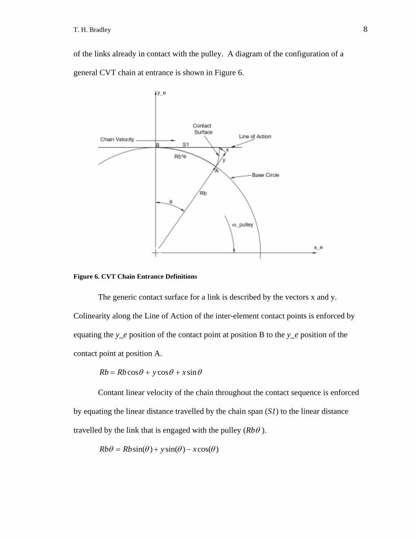
of the links already in contact with the pulley. A diagram of the configuration of a
general CVT chain at entrance is shown in Figure 6.
Figure 6. CVT Chain Entrance Definitions
The generic contact surface for a link is described by the vectors x and y.
Colinearity along the Line of Action of the inter-element contact points is enforced by
equating the y_e position of the contact point at position B to the y_e position of the
contact point at position A.
θθθ sincoscos xyRbRb ++=
Contant linear velocity of the chain throughout the contact sequence is enforced
by equating the linear distance travelled by the chain span (S1) to the linear distance
travelled by the link that is engaged with the pulley (Rbθ ).
)cos()sin()sin( θθθθ xyRbRb −+=

T. H. Bradley 9
Solving for x(θ ) and y(θ ) gives the equation of the pin contact surface that
satisfies the Law of Conjugate Action. The solutions are the equations of the involute of
circle of radius, Rb [Khiralla 1976]:
[ ])cos()sin( θθθ −= Rbx
[ ])sin()cos( θθθ += Rby .
Under the assumptions of this analysis, giving the inter-element contact surface
the shape of this involute satisfies the Law of Conjugate Action minimizes polygonal
action at a single radius. Again, this analysis assumes a simplified motion of the chain
span but is valid as an illustration of the theory and general design configuration for the
involute CVT chain
Limitations of the Continuous Static Chain Model The contact surface involute can only be optimized for one radius and therefore
only one ratio. The value assigned to Rb defines the radius at which the equilibrium line
of action is tangent to the pulley contact circle, where polygonal action is minimized.
This condition is illustrated in Figure 7. As the equilibrium radius of the chain increases
with changing ratio, the positions of the Line of Action and the line tangent to the chain
contact circle diverge. This effect forces the chain to enter the pulley at a radius not
equal to the radius of the equilibrium contact circle. An accurate description of this effect
is necessary to choose a value of Rb that minimizes polygonal action over a wide span of
ratios.

T. H. Bradley 10
Figure 7. Involute Chain, Line of Action Tangent to Contact Circle [van Rooij 1996]
The goal of the design of the involute contact CVT chain is to transmit entrance
effects upstream to lessen the impact of the pin to the CVT pulley. Understanding these
entrance effects demands a second, more detailed geometric model of the chain span.
Discrete Static Chain Model
The objective of the Discrete Static Chain Model is to address the limitations of
the Continuous Static Chain Model, to analyze the tradeoffs in contact surface design and
to compare the behavior of the involute CVT chains with pinned-joint CVT chains. In
order to expand the validity of the static chain CVT model to encompass these subjects,
the model will be expanded to represent five chain elements in the entrance zone of the
pulley. Modeling assumptions are as follows:
• As before, static conditions, rigid elements and pulleys, and no exit effects
transmitted from the upstream side of the chain span.
• Now, the position and rotation of the five elements are defined by three
independent coordinates (x, y, θ).

T. H. Bradley 11
• The angular position of the 6th link upstream of the analysis is assumed to
be tangential to the contact circle, ( 0) =iθ .
• The chain does not creep or slip while in contact with the pulleys.
• All pin to pulley contact occurs at the equilibrium radius.
Formulation of Equations For this analysis, new definitions for the intra-element geometry of the chain are
required. The location of the link contact surfaces are described using the vectors shown
in Figure 8. A_b and B_b describe the location of the contact points for the link in a
straight chain span using body coordinates. The vector
describes the shape of the
involute from the end of A_b and B_b, and is also in body coordinates.
yx
Figure 8. Chain Element Vector and Coordinate Definitions (as in [van Rooij 1996])
The geometry of the CVT chain system is described using two equations per
chain element contact.
Equation (1) dictates that the inter-element contact points are colocated, that the
position of the upstream contact point in the y_e direction for link i is equal to the y_e
position of the upstream contact point for link i+1:
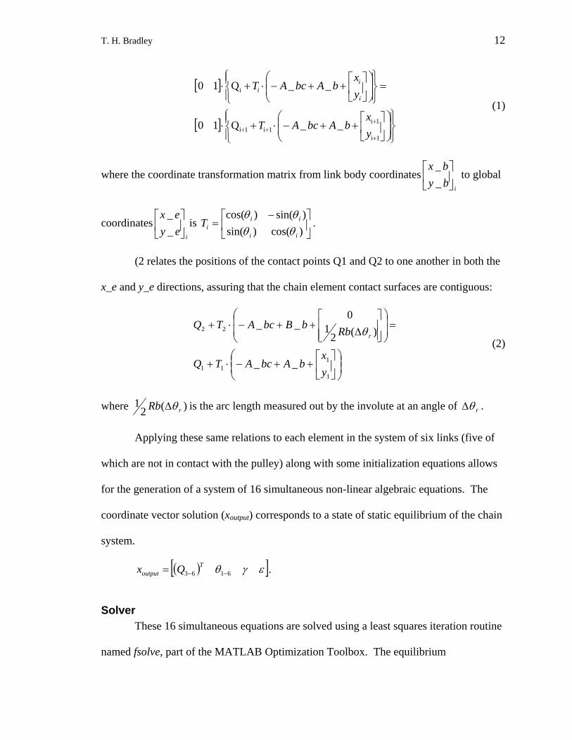
T. H. Bradley 12
[ ]
[ ]
++−⋅+⋅
=
++−⋅+⋅
+
+++
1i
1i1i1i
i
__ Q10
__ Q10
yx
bAbcAT
yx
bAbcATi
ii
(1)
where the coordinate transformation matrix from link body coordinates to global
coordinates is T .
ibybx
__
ieyex
__
−=
)cos()sin()sin()cos(
ii
iii θθ
θθ
(2 relates the positions of the contact points Q1 and Q2 to one another in both the
x_e and y_e directions, assuring that the chain element contact surfaces are contiguous:
++−⋅+
=
∆
++−⋅+
1
111
22
__
)(21
0__
yx
bAbcATQ
RbbBbcATQrθ
(2)
where )(21
rRb θ∆ is the arc length measured out by the involute at an angle of rθ∆ .
Applying these same relations to each element in the system of six links (five of
which are not in contact with the pulley) along with some initialization equations allows
for the generation of a system of 16 simultaneous non-linear algebraic equations. The
coordinate vector solution (xoutput) corresponds to a state of static equilibrium of the chain
system.
( )[ ]εγθ 6163 −−= Toutput Qx .
Solver These 16 simultaneous equations are solved using a least squares iteration routine
named fsolve, part of the MATLAB Optimization Toolbox. The equilibrium

T. H. Bradley 13
configuration for the chain span is calculated at discrete points encompassing the
movement of one element length. Derivative discontinuity in the results of the static
CVT chain model is present due to the very small values being examined, and the
iterative nature of these solutions. A copy of the program used to perform these
calculations is presented in Appendix 1.
Results Figure 9 shows the general configuration of the CVT chain at entrance as
calculated using the Discrete Static Chain Model. In this figure, the motions of the chain
elements are from left to right and the rotation of the pulley is clockwise. The chain is in
permanent contact with the pulley after contacting the pulley at the labeled points. The
geometry of the involute contact chain simulates the geometry of the GCI CVT chain.
For comparison, the path of a chain with pinned inter-element contacts is also illustrated.
The pinned contact chain configuration represents a chain with a pin connection between
chain elements, similar to the chain shown in Figure 10. Both configurations are
modeled with equal pitch.

T. H. Bradley 14
Figure 9. Chain Path and Definitions for Involute and Pinned CVT Chains (Vertical axis is exaggerated for clarity)
Figure 10. Pinned Joint CVT Chain, Line of Action Displaced from Tangent Line
Initially, the results of this simulation will rely on two geometric quantities from
the static chain configuration to predict the type and degree of polygonal action. The
quantity dh, defined in Figure 9, is related to the occurrence of the semi-static type of
polygonal action. The angle of incidence, also defined in Figure 9, is related to the force
experienced by the chain element at impact to the pulley, and therefore is an indicator of
the dynamic type of polygonal action. Both dh and the angle of incidence will be
determined from calculation of the equilibrium configuration of the CVT chain in order
to characterize the type and magnitude of polygonal action present in each chain design.
CHARACTERIZATION OF SEMI-STATIC POLYGONAL ACTION - As can be seen in
Figure 9, the position and configuration of the involute contact surface chain are very
different from the position and configuration of the pinned contact chain. Each line
represents the path in space of the pin-to-pulley contact point. For the involute contact
chain, the impact of the chain pin with the pulley occurs at a y-position of 34.9 mm, ie. dh
is equal to 0. For the pinned contact chain, the pin-to-pulley contact occurs at a y_e
T. H. Bradley 15
position of 34.6 mm, ie. dh = 0.3 mm. Because dh has been chosen as an indicator of
semi-static polygonal action, this simulation indicates that the involute contact chain
should exhibit less semi-static polygonal action than the pinned contact chain at a contact
radius of 34.9 mm.
Figure 11. Y-direction Distance of Impact from Tangent for Involute and Roller CVT Chains
Figure 11 shows the relationship between the equilibrium radius of the chain and
the distance of the point of impact from tangent, dh. Although dh for the involute chain
does increase slightly with increasing pulley radius, at all radii dh for the involute chain is
smaller than dh for the pinned contact chain. This suggests that the involute contact
chain will exhibit less semi-static polygonal action than the pinned contact chain at all
radii.
CHARACTERIZATION OF DYNAMIC POLYGONAL ACTION - Figure 12 shows the
relationship between the equilibrium radius of the CVT chain and the angle of incidence
of the chain element as it comes in contact with the pulley contact circle. As should be
expected, the angle of incidence decreases at higher pulley radii. Also, the angle of
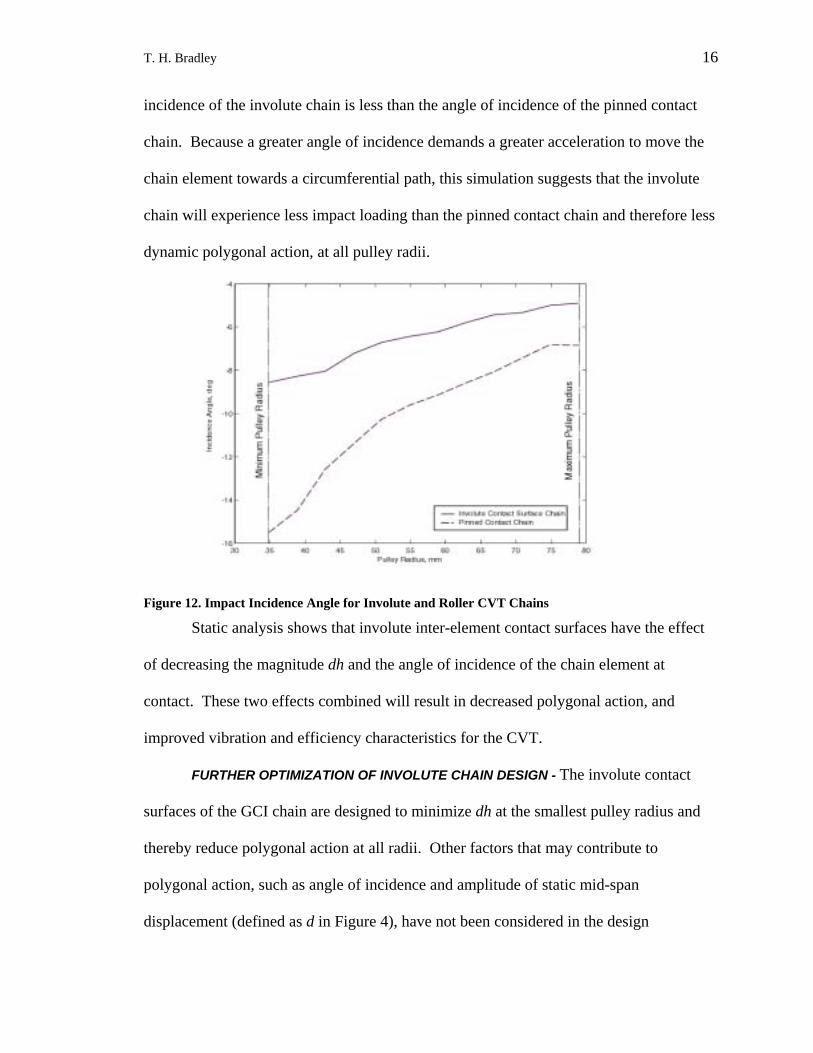
T. H. Bradley 16
incidence of the involute chain is less than the angle of incidence of the pinned contact
chain. Because a greater angle of incidence demands a greater acceleration to move the
chain element towards a circumferential path, this simulation suggests that the involute
chain will experience less impact loading than the pinned contact chain and therefore less
dynamic polygonal action, at all pulley radii.
Figure 12. Impact Incidence Angle for Involute and Roller CVT Chains
Static analysis shows that involute inter-element contact surfaces have the effect
of decreasing the magnitude dh and the angle of incidence of the chain element at
contact. These two effects combined will result in decreased polygonal action, and
improved vibration and efficiency characteristics for the CVT.
FURTHER OPTIMIZATION OF INVOLUTE CHAIN DESIGN - The involute contact
surfaces of the GCI chain are designed to minimize dh at the smallest pulley radius and
thereby reduce polygonal action at all radii. Other factors that may contribute to
polygonal action, such as angle of incidence and amplitude of static mid-span
displacement (defined as d in Figure 4), have not been considered in the design
T. H. Bradley 17
optimization. This small scope of the GCI design optimization is a result of the
limitations of preexisting static models of the GCI CVT chain.
The static model designed and implemented as part of this research allows for
calculation of the static equilibrium configuration of the CVT chain at various
configurations. This flexibility allows design optimization to include minimization of
other factors that are contributors to polygonal action. This section of the results will
show how the design of the involute contact chain can be improved for lower dh, lower
angle of incidence and lower midspan vibration amplitude using the Discrete Static Chain
Model described above. Although this section of the static simulation results is
somewhat of an aside, it provides insight into the tradeoffs present in optimization of the
involute contact surfaces.
Figure 13 shows the effect that varying the involute base radius, Rb, has on the
location of contact of the chain to the pulley. As should be expected, the simulation
shows that the pinned contact chain impacts the pulley under the line tangent to the
pulley contact circle at point 1. As shown in Figure 13, the involute chain with a base
radius, Rb, of 56 mm impacts exactly at the tangent line at position 2. By increasing the
base radius of the involute, the chain configuration is changed so that the chain element
contacts on the other side of the pulley at position 3. In this case, dh is still positive
because the chain has impacted below the tangent line.

T. H. Bradley 18
Figure 13. Chain Path for Involute Chains of Different Base Radii
By increasing Rb to greater than 56 mm, polygonal action can be further reduced
in two ways. First, as shown in Figure 13, the angle of incidence of the pin-to-pulley
impact is reduced with increasing Rb. Angle of incidence has earlier been equated to
dynamic polygonal action. The second benefit of a configuration incorporating a larger
Rb is not evident without an investigation of the effect of ratio on the quantity dh for
various values of Rb. As shown in Figure 14, the average value of dh at all radii for the
involute chain of Rb = 75mm is 62% smaller than the value for the involute chain with
Rb = 56mm. A smaller value of dh means lower impact forces and less semi-static
polygonal action.

T. H. Bradley 19
Figure 14. Y-direction Distance of Impact from Tangent for Involute Chains of Various Rb
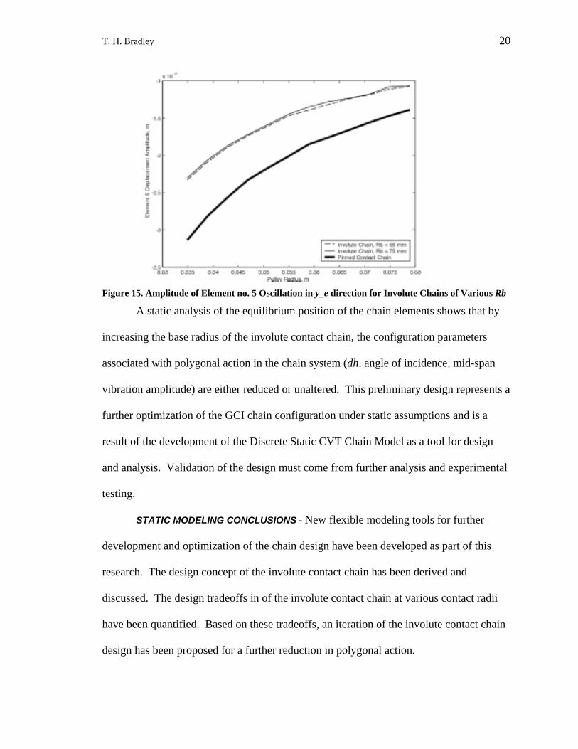
As a final design configuration check, Figure 15 shows the amplitude of
movement of the chain element 4 links upstream from the impacting chain element. The
chain span displacement amplitude, represented analytically by the peak-to-peak vertical
displacement of element no. 5, does not increase with increased values of Rb. This
suggests that the benefits exhibited by the chain with Rb > 56mm do not come at the
expense of chain span displacement.
T. H. Bradley 20
Figure 15. Amplitude of Element no. 5 Oscillation in y_e direction for Involute Chains of Various Rb
A static analysis of the equilibrium position of the chain elements shows that by
increasing the base radius of the involute contact chain, the configuration parameters
associated with polygonal action in the chain system (dh, angle of incidence, mid-span
vibration amplitude) are either reduced or unaltered. This preliminary design represents a
further optimization of the GCI chain configuration under static assumptions and is a
result of the development of the Discrete Static CVT Chain Model as a tool for design
and analysis. Validation of the design must come from further analysis and experimental
testing.
STATIC MODELING CONCLUSIONS - New flexible modeling tools for further
development and optimization of the chain design have been developed as part of this
research. The design concept of the involute contact chain has been derived and
discussed. The design tradeoffs in of the involute contact chain at various contact radii
have been quantified. Based on these tradeoffs, an iteration of the involute contact chain
design has been proposed for a further reduction in polygonal action.
T. H. Bradley 21
DYNAMIC MODEL OF AN INVOLUTE CVT CHAIN
A dynamic simulation of the CVT chain will be used to determine the dynamic
effectiveness of involute contact surfaces in reducing vibration and polygonal action in
CVT chains, to verify the effectiveness of the design of the involute CVT chain. The
dynamic chain model is designed to simulate the geometry of the 30 mm GCI CVT chain.
Constitutive Component Models
Chain Model Description and Validation Various methods have been investigated for simulation and analysis of the motion
of chain drives, but they can be divided grossly into static and dynamic analyses. Static
analyses consist of determining chain to sprocket contact conditions and calculating
forces and positions of chain links based on static calculations as performed above.
Dynamic analyses consist of devising a chain model and solving for forces on the chain
using dynamic calculations. Assumptions used in construction of the dynamic chain
model determine which aspects of chain dynamics can be studied. [Ariaratnam 1987]
modeled the chain span as a one-dimensional continuous compliant string to study
dynamic chain stability. Others have studied chain polygonal action by modeling the
chain with four-bar linkages. [Bothwell 1987], [Srnik 1997] and [Troedsson 2001]
formulate dynamic equations using a multibody scheme with compliant constraints.
Multibody dynamic simulations have the advantage of being able to capture polygonal
action, chain inter-link dynamics, chain to pulley contact and entrance and exit effects.
CHAIN MODEL DESCRIPTION - Because the goal of this analysis is to evaluate
sources of vibration from all of these sources, a multibody dynamic simulation with
compliant constraints was chosen for this study. A planar rigid body is used to model

T. H. Bradley 22
each element of the CVT chain. The element has 3 degrees of freedom corresponding to
two in translation and one in rotation in the plane. The chain elements are coupled to
adjacent links with compliance and damping elements that represent elasticity and
damping in the inter-link bearings. These elements apply forces to the links in both the
x_b and y_b directions in the plane based on the differential displacement and velocities
of adjacent links. Differential rotation of the link does not produce reaction forces.
Figure 16. X and Y Direction Link Compliance Model
A multilateral contact model is used to describe the compliance between the strip
of element i and the pin of element i+1. The compliance between chain elements is
modeled as the series sum of compliance from Hertz contact compliance, bending of the
pin and link and elastic extension of the link plates. Hertzian contact between the chain
links and the pins is not considered.
HERTZ CONTACT COMPLIANCE - For the Hertz contact compliance, the strip is
modeled as an elastic flat half space and the pin is modeled as an elastic cylinder. From
[Johnson 1985], the contact displacement δ , of a cylinder in contact with a planar
surface is:
( )[ ]1)/4ln(21 2
−−
= aRE
Pπ
υδ (3)
where the semi-contact-width is

T. H. Bradley 23
*4
EPRa π= (4)
ELASTIC PIN BENDING - The pin is loaded by contact forces from the pulleys and
by contact forces from the chain links. The position and magnitude of the loads
transmitted to the pin by the links are determined by the geometry of the joint. Because
the pattern of the chain links repeats every three links there are three different loading
conditions for the chain pin which must be examined to derive a global or averaged
compliance. The joint configuration and loading conditions for Joint 2 are shown in
Figure 17. Each link-to-pin contact is represented as a point load, located at the same
position as the contact point relative to the x-axis of the pin.1
Element i
y
x
P
P
P
P
Element i+1
Joint 1 Joint 2 Joint 3
Figure 17. Element Definitions and Pin Loading Diagrams
Bending of the pin is modeled as the bending of a linear elastic, simple, slender
beam under multiple point loading conditions with fully constrained ends. The
T. H. Bradley 24
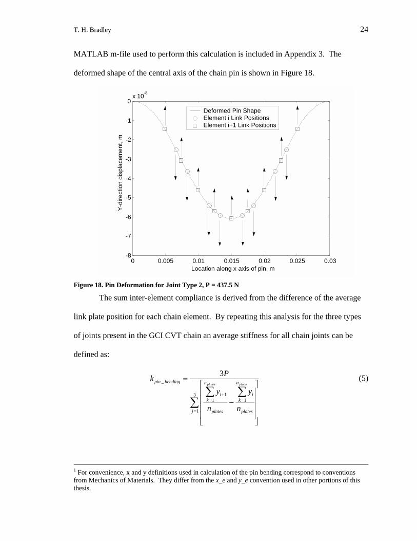
MATLAB m-file used to perform this calculation is included in Appendix 3. The
deformed shape of the central axis of the chain pin is shown in Figure 18.
0 0.005 0.01 0.015 0.02 0.025 0.03-8
-7
-6
-5
-4
-3
-2
-1
0 x 10 -8
Location along x-axis of pin, m
Y-di
rect
ion
disp
lace
men
t, m
Deformed Pin Shape Element i Link Positions Element i+1 Link Positions
Figure 18. Pin Deformation for Joint Type 2, P = 437.5 N
The sum inter-element compliance is derived from the difference of the average
link plate position for each chain element. By repeating this analysis for the three types
of joints present in the GCI CVT chain an average stiffness for all chain joints can be
defined as:
∑∑∑
=
==+
−
=
3
1
111
_3
j plates
n
ki
plates
n
ki
bendingpin
n
y
n
y
Pkplatesplates
(5)
1 For convenience, x and y definitions used in calculation of the pin bending correspond to conventions from Mechanics of Materials. They differ from the x_e and y_e convention used in other portions of this thesis.

T. H. Bradley 25
where j is the joint number, i is the element number, y is the displacement of the pin at
each link and nplates is the number of links per element.
ELASTIC LINK EXTENSION - Elastic extension of the link plates is modeled as a
beam under simple tension, where EAn
PL
plates
=δ , and nplates is the number of parallel link
plates per chain element. As shown in Figure 19, the elastic extension of the link plates
is more compliant than the other deformation mechanisms. All compliances are very
linear over the range of applied forces encountered in the simulation, and are modeled as
linear.
0 500 1000 1500 2000 2500 3000 3500 4000
0
2
4
6
8
10
12
14
16
18
20x 10
-7
Applied Force, N
Dis
plac
emen
t, m
Pin Bending Compliance Model Hertz Line Contact Compliance Model Link Elastic Elongation Compliance Model
Figure 19. Modeled Sources of Inter-Element Compliance
The compliance that is derived from the series sum of these models is
multilaterally applied in both the x and y-directions. The links are assembled into a chain
of 75 identical elements with identical compliances.
T. H. Bradley 26
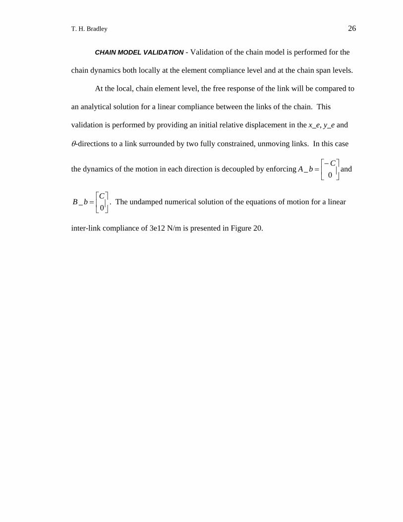
CHAIN MODEL VALIDATION - Validation of the chain model is performed for the
chain dynamics both locally at the element compliance level and at the chain span levels.
At the local, chain element level, the free response of the link will be compared to
an analytical solution for a linear compliance between the links of the chain. This
validation is performed by providing an initial relative displacement in the x_e, y_e and
θ-directions to a link surrounded by two fully constrained, unmoving links. In this case
the dynamics of the motion in each direction is decoupled by enforcing and
. The undamped numerical solution of the equations of motion for a linear
inter-link compliance of 3e12 N/m is presented in Figure 20.
−=
0_
CbA
=
0_
CbB

T. H. Bradley 27
0 0.5 1 1.5 2 2.5 3 3.5 4
x 10-7
-5
0
5 x 10 -10
Y-di
rect
ion
posi
tion,
m
0 0.5 1 1.5 2 2.5 3 3.5 4
x 10-7
-5
0
5 x 10 -10 X-
dire
ctio
n po
sitio
n, m
0 0.5 1 1.5 2 2.5 3 3.5 4
x 10-7
-0.2 -0.1
0 0.1 0.2
Thet
a di
rect
ion
posi
tion,
rad
Time, sec
Figure 20. Chain Element Natural Period Validation
In this test case the moment of inertia of the link, I_link, has been chosen to make
the period of rotational oscillation equal to the period of linear oscillation. The period of
oscillation can be analytically calculated as
rotlin klinkI
kM _22 ππτ == ,
where the rotational compliance
linrot krk 2= .
The calculated period of oscillation is 2.56e-7 seconds, and the simulated period
of oscillation is 2.56e-7 seconds. After 10 oscillations the energy of the system is
conserved to within 0.3%. For a linear compliance with no damping, the equations are

T. H. Bradley 28
proven correct and the model is considered validated at the link level against the
analytical solution.
Globally, the model will be validated by comparing the numerical period of
oscillation of a representative chain span to an analytical solution. Eighteen discrete
elements with pinned contact surfaces are assembled into a chain between two fully
constrained, immovable elements. The chain is provided an initial half period sinusoidal
displacement and the equations of motion are solved using an ordinary differential
equation solver. Figure 21 shows the first mode of the chain vibration for the 18 element
discrete chain. The shape and period of oscillation of this mode will be validated against
an analytical, continuous solution.
0 0.02 0.04 0.06 0.08 0.1 0.12 0.14 0.16 0.18 0.2-0.01
-0.008
-0.006
-0.004
-0.002
0
0.002
0.004
0.006
0.008
0.01
X-position, m
Y-po
sitio
n, m
Figure 21. Chain Mode Shapes and CG Locations
By approximating the chain as a continuous heavy string under tension, the
natural first order period of oscillation is defined as
tenscont Tn
lT ρ2= .

T. H. Bradley 29
Comparison of the numerical and analytical periods of oscillation for the chain
span shows acceptable correlation considering that the analytical solution is an
approximation of the behavior of the discrete chain.
Table 1. Comparison of Numerical and Analytical Span Vibration Solutions
Chain Tension T tens [N]
Chain Density
ρ [kg/m]
Numerical Natural Period
T num [sec]
Analytical Natural Period
T cont [sec]Percent
Difference275 1.081 0.020 0.022 9.1%2748 0.992 0.0067 0.0073 7.8%
The global inter-link dynamics of the chain model are considered validated
against a simple analytical model.
Contact Model Description and Validation Two fundamental tools exist for modeling of impact with friction in rigid body
systems: impulse-momentum relations and compliant contact modeling [Stronge 2000].
Impulse-momentum relations are only applicable to a multi-body system where the
contact compliance is either very high or very low in comparison to inter-body
compliances, because this allows the assumption of simultaneous or sequential impact.
Because the compliance of contact between the chain and the pulleys is of the same order
as the compliance of contact between the chain links, strict impulse-momentum relations
will produce erroneous results for a multibody chain simulation. Instead, a compliant
contact modeling approach is required where each individual contact for each body is
represented by a discrete compliance; a local contact compliance is required for both the
inter-element contact and the pin to pulley contact [Stronge 2000]. The three main
disadvantages of compliant contact modeling for numerical simulation of multibody
contact dynamics are that it often leads to stiff differential equations, that oscillations can

T. H. Bradley 30
occur under conditions of permanent contact and that a continuous friction law is often
needed to maintain constant causality under slip-stick contact [Abadie 2000]. In the case
of this simulation these problems are resolved to an acceptable degree. The nature of the
differential equations are discussed in the section titled Formulation of Equations, and
contact oscillations and friction laws are discussed in the section titled Contact Model
Description and Validation.
CONTACT MODEL DESCRIPTION - For this simulation, a local contact compliance
model is used between the pulley sheaves and the chain element. The contact compliance
is modeled as the series sum of a Hertzian contact model and a linear elastic pin
compliance model. A diagram of the pin to pulley contact model is shown in Figure 22.
The point where the pin contact with the pulley is massless and its motion is restricted to
translation in the z-direction.
Figure 22. Pin Compliance Model
A spherical Hertzian contact model is used to represent the contact forces between
the chain pins and the pulley sheaves. Although Hertzian contact relations are based on a
semi-static analysis and impact mechanics are by nature dynamic, Hertzian contact
relations are a widely used approximation of impact compliance [Stronge 2000] [Kraus
T. H. Bradley 31
1997]. In the case of link to pulley contact, both the pulley sheaves and the pin contact
surfaces are approximated as large radius spheres.
Sample contact laws for inelastic, spherical, Hertzian contact are:
23
δκ scompF = [Abadie 2000]
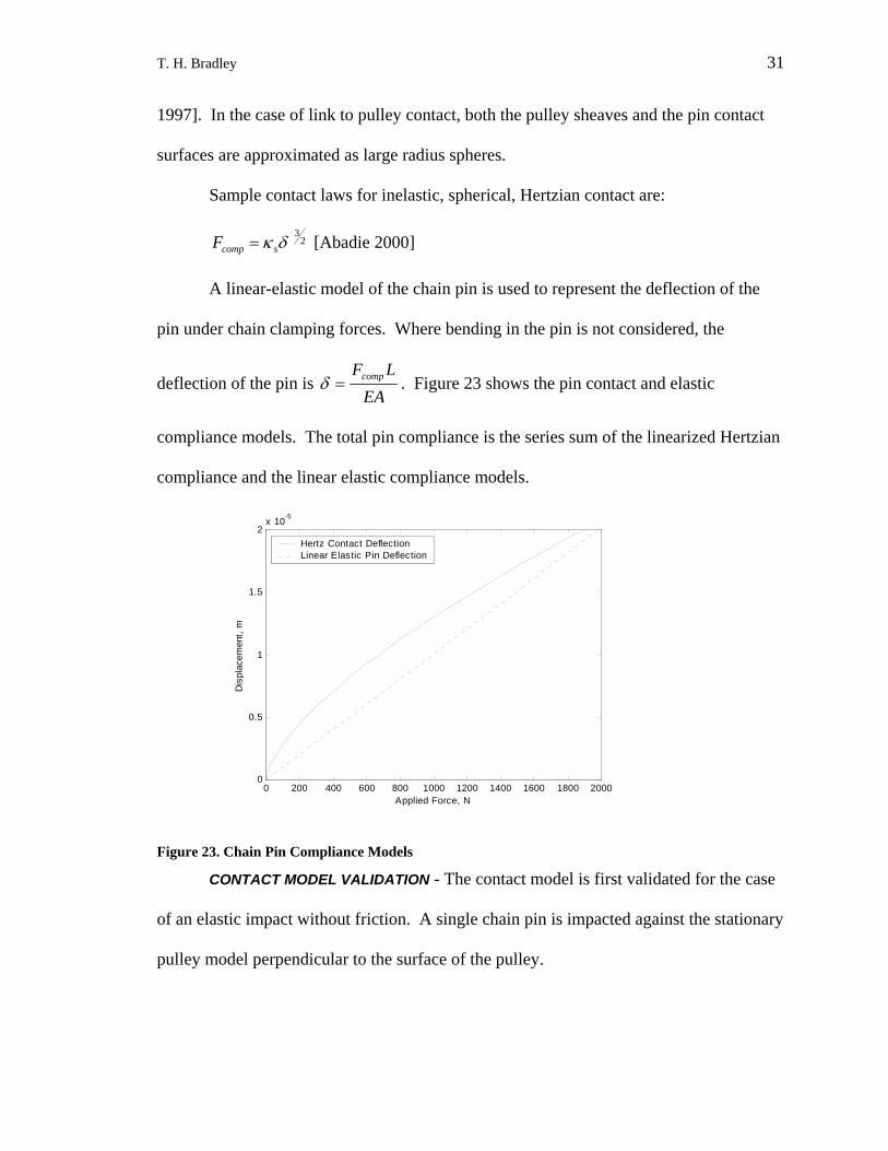
A linear-elastic model of the chain pin is used to represent the deflection of the
pin under chain clamping forces. Where bending in the pin is not considered, the
deflection of the pin is EA
LFcomp=δ . Figure 23 shows the pin contact and elastic
compliance models. The total pin compliance is the series sum of the linearized Hertzian
compliance and the linear elastic compliance models.
0 200 400 600 800 1000 1200 1400 1600 1800 20000
0.5
1
1.5
2x 10⁻⁵
Applied Force, N
Dis
plac
emen
t, m
Hertz Contact Deflection Linear Elastic Pin Deflection
Figure 23. Chain Pin Compliance Models
CONTACT MODEL VALIDATION - The contact model is first validated for the case
of an elastic impact without friction. A single chain pin is impacted against the stationary
pulley model perpendicular to the surface of the pulley.
T. H. Bradley 32
5 5.1 5.2
x 10-4
-8
-6
-4
-2
0x 10-5
y-di
rect
ion
posi
tion,
mTime, sec
5 5.1 5.2
x 10-4
-0.1
-0.05
0
0.05
0.1
y-di
rect
ion
mom
entu
m, k
g-m
/s
Time, sec
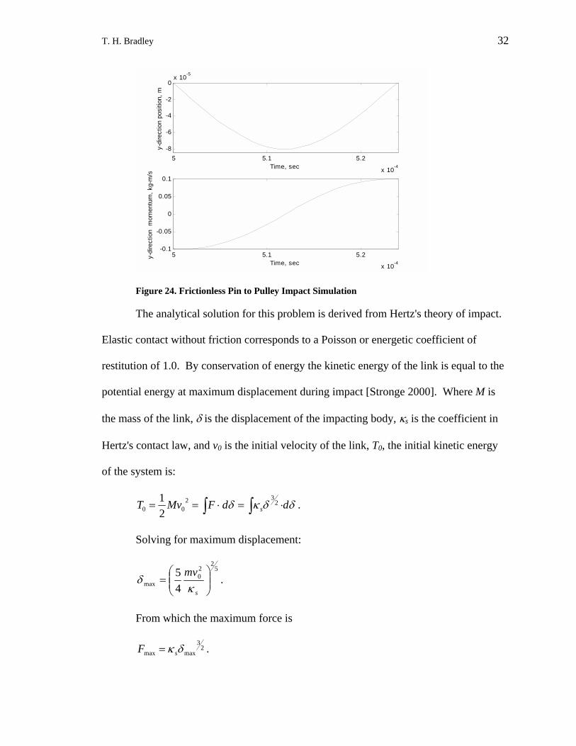
Figure 24. Frictionless Pin to Pulley Impact Simulation
The analytical solution for this problem is derived from Hertz's theory of impact.
Elastic contact without friction corresponds to a Poisson or energetic coefficient of
restitution of 1.0. By conservation of energy the kinetic energy of the link is equal to the
potential energy at maximum displacement during impact [Stronge 2000]. Where M is
the mass of the link, δ is the displacement of the impacting body, κs is the coefficient in
Hertz's contact law, and v0 is the initial velocity of the link, T0, the initial kinetic energy
of the system is:
δδκδ ddFMvT s∫∫ ⋅=⋅== 232
00 21 .
Solving for maximum displacement:
52
20
max 45
=
s
mvκ
δ .
From which the maximum force is
23
maxmax δκ sF = .
T. H. Bradley 33
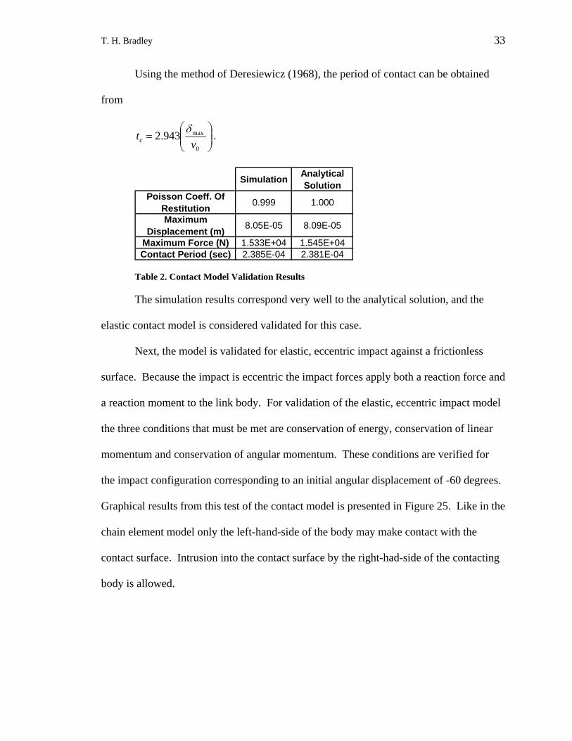
Using the method of Deresiewicz (1968), the period of contact can be obtained
from
=
0
max943.2v
tcδ .
Simulation Analytical Solution
Poisson Coeff. Of Restitution 0.999 1.000
Maximum Displacement (m) 8.05E-05 8.09E-05
Maximum Force (N) 1.533E+04 1.545E+04Contact Period (sec) 2.385E-04 2.381E-04
Table 2. Contact Model Validation Results
The simulation results correspond very well to the analytical solution, and the
elastic contact model is considered validated for this case.
Next, the model is validated for elastic, eccentric impact against a frictionless
surface. Because the impact is eccentric the impact forces apply both a reaction force and
a reaction moment to the link body. For validation of the elastic, eccentric impact model
the three conditions that must be met are conservation of energy, conservation of linear
momentum and conservation of angular momentum. These conditions are verified for
the impact configuration corresponding to an initial angular displacement of -60 degrees.
Graphical results from this test of the contact model is presented in Figure 25. Like in the
chain element model only the left-hand-side of the body may make contact with the
contact surface. Intrusion into the contact surface by the right-had-side of the contacting
body is allowed.

T. H. Bradley 34
Figure 25. Frictionless Contact Model Validation
Conservation of energy is verified by calculating the Poisson coefficient of
restitution. A Poisson coefficient of restitution of 1.0 represents perfect energy
conservation. Conservation of linear and angular momenta are verified using the
equations of motion of a rigid body acted on by an impulse dP. In the y-direction,
, and in rotation, vMdP ∆= dPbAlinkI m ×=⋅ __ θ& . Using the results of the simulation
the magnitude of the impulse dP can be calculated from both equations. Conservation of
linear and angular momenta demands that the calculated impulses be equal.
Table 3. Rigid Body Contact Model Validation Results
Poisson Coeff. of Restitution 1.01
Y-direction Calculated dP
(kg-m/s)0.1610
Rotational Calculated dP
(kg-m/s)0.1598

T. H. Bradley 35
As seen in Table 3, the results of the simulation obey conservation of energy and
momentum. The impulse in the rotational direction is equal to the impulse in the
translational direction to within 1%, and the energetic coefficient of restitution is equal to
approximately 1.0. On the basis of validation under colinear and eccentric rigid body
contact, the model is considered validated against the analytical solutions.
Friction Model Description and Validation The precise characteristics of the friction interface between the links and sheaves
in a chain CVT transmission are unknown. In belt CVTs, slip-stick friction is present in
the contact between the belt elements and the sheaves of the transmission. Several
friction models have been proposed to represent this interface in belt CVTs, including
Coulombic [Gerbert 1984; Fujii 1993; Kobayashi 1998] and elastohydrodynamic friction
[Micklem 1994], but it cannot lightly be presumed that the friction characteristics of a
CVT chain are the same as those of a CVT belt. The contact surface in a CVT chain is,
in general, characterized by lower slip rates, higher contact pressures, and higher impact
forces than in CVT belts. Published experimental data for friction measurements in CVT
chains are, as yet, non-existent. In constructing a simulation model of a PIV CVT chain,
Srnik and Pfeiffer [Srnik 1994] use both a strict Coulomb friction model and a continuous
approximation of Coulomb friction with similar results. Still, in order to improve the
adaptability of the model and in an attempt to capture all dynamics of relevance, a slip-
stick friction model is preferable.
FRICTION MODEL DESCRIPTION - In this simulation, a slip-stick friction model
will be used that is based on the algorithm of Leine et al. [Leine 1998]. This algorithm
avoids the physical and numerical problems that are associated with strict Coulomb

T. H. Bradley 36
friction models and their continuous approximations. The equations of state produced
with this algorithm are non-stiff, ordinary differential equations with constant causality.
The Leine algorithm is based on the friction model introduced by Karnopp
[Karnopp 1985]. Karnopp friction defines a small band of relative velocity centered at
zero with width of twice DV. Outside of this velocity band, the system is assumed to slip.
Inside of this band, if the applied force on the system is less than breakaway friction
force, the system will stick. If the force on the system is greater than the breakaway
friction force, the system will transition to slip. With Karnopp friction, the system carries
a small velocity error when stuck. Under stick, the algorithm of Leine et. al. forces the
velocity of the system to zero to avoid the error and numerical instability associated with
Karnopp friction.
0.11 0.12 0.13 0.14 0.15 0.16-0.02
0
0.02
0.04
0.06
0.08
0.1
0.12
0.14
0.16
0.18
X-d
irect
ion
Mom
entu
m, k
g-m
/s
Time, sec
Analytical Solution Karnopp Algorithm Leine et. al. Algorithm
DV
Figure 26. Friction Law Comparison
The behavior of a link sliding to a stop in contact with the CVT pulley is shown in
Figure 26. In the slip regime, all solutions are identical. At the transition to stick, the
Coulomb solution continues to zero velocity, the Karnopp solution remains at the small

T. H. Bradley 37
velocity DV = 0.1 m/s, and the solution of Leine et. al. converges to zero under the action
of a fictitious sticking force.
An additional benefit to a slip stick algorithm is that at velocities under DV, all
forces other than the fictitious sticking force are cancelled. Canceling these excitations
eliminates the numerical instabilities associated with compliant contact modeling, as
discussed in the section titled Contact Model Description and Validation. The friction
model that is validated and used in the dynamic chain CVT simulation is the model of
Leine et al.
FRICTION MODEL VALIDATION - The friction model is validated by comparison to
analytical solutions using strict Coulomb friction. The first validation test is performed
by giving a 2-DOF chain link model an initial velocity and allowing dynamic friction to
drag the link to a stop. The chain link is constrained by reaction forces from a pulley
model of infinite radius and the applied force of gravity as shown in Figure 27. A
comparison of the friction model to the analytical solution is presented graphically in
Figure 26.
y
x Vo
M g y
z
Figure 27. Chain Link Contact Configuration
T. H. Bradley 38
The comparison shows that the friction model is equivalent to the analytical
solution until the sticking velocity is reached. The quantity DV must therefore be chosen
to be lower than any velocity of interest.
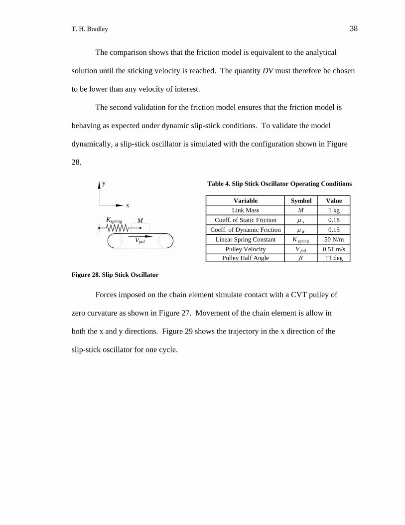
The second validation for the friction model ensures that the friction model is
behaving as expected under dynamic slip-stick conditions. To validate the model
dynamically, a slip-stick oscillator is simulated with the configuration shown in Figure
28.
y
x
Kspring M
Vpul
Figure 28. Slip Stick Oscillator
Table 4. Slip Stick Oscillator Operating Conditions
Variable Symbol ValueLink Mass M 1 kg
Coeff. of Static Friction µ s 0.18Coeff. of Dynamic Friction µ d 0.15
Linear Spring Constant K spring 50 N/mPulley Velocity V pul 0.51 m/s
Pulley Half Angle β 11 deg
Forces imposed on the chain element simulate contact with a CVT pulley of
zero curvature as shown in Figure 27. Movement of the chain element is allow in
both the x and y directions. Figure 29 shows the trajectory in the x direction of the
slip-stick oscillator for one cycle.

T. H. Bradley 39
Figure 29. Slip Stick Oscillator Trajectory
From point 1 to point 2, the link is stuck to the moving surface. The relative
velocity of the link to the surface is zero and the displacement of the link is increasing
at a rate of Vpul. At point 2, the force from the displaced spring is equal to the force of
static friction, and the link begins to slip relative to the moving surface. Analytically,
using Coulomb's law of friction this transition from stick to slip should occur at a
displacement of:
mK
Mgxspring
s 185.0)sin(
==µ
β.
Numerically, this transition occurs at 0.188m. At point 3, the relative and
absolute acceleration of the link is zero. Again, from Coulomb's law of friction,
mK
Mgxspring
d 154.0)sin(
==µ
β

T. H. Bradley 40
Numerically, this state occurs at a position of 0.154m. At point 4 the link
sticks and the cycle repeats. From analysis of the slip-stick oscillator the two-
dimensional friction model is validated to the Coulomb friction law. The stability and
accuracy of the two-dimensional friction law under slip-stick conditions and under
conditions of continuous contact is also verified.
Modeled Link and Pulley Characteristics The link element and pulley characteristics are chosen to emulate the GCI 2L
CVT chain installed in a Nissan 2L CVT. Inertias and masses for the links and
pulleys are measured or calculated from the actual components. Compliances for the
system are calculated from the models of the contacts in the system. Tension in the
CVT chain is produced by varying the spacing between the two sheaves of the CVT
pulley. Pulleys are rigid and un-skewed. Pulley rigidity is an important
simplification because pulley flex and skew determine the dynamics of the chain in
contact with the pulley. For proper modeling of the dynamics of the chain in contact
with the pulleys, a model of pulley deformation is required [Gerbert 1996; Srnik
1997; Srnik 1999]. Here, this simplification is justified because the focus of this
model is chain span dynamics instead of chain/pulley interactions or dynamics.
The models for the 75 element chain and two CVT pulleys are then assembled
into a global mathematical model of the CVT variator (CVT chain and pulley
system).

T. H. Bradley 41
Mathematical Formulation
Formulation of Equations To formulate equations, definitions of the applicable coordinate systems are
required. Local coordinate systems are established for each chain element, and a
global Newtonian coordinate frame is established. In the most general representation,
the model is formulated in the form of equations of motion in the global coordinate
frame.
[ ] [ ] ( )[ ] ( )[ ] NqqqqhqM ℜ∈=++⋅ 0,, &&&& λ
Where is the positive definite mass matrix for the set of minimal
coordinates [ , in the global coordinate system. The vector of states, [ , is of the
form
[M
]
]
q ]q
[ ] [ ]Tpulleypulleylinksnlinksnlinksn ii
yyxxq θθθθ &ΛΛΛ _1_1_1= .
The vector [ represents the applied forces due to inter-element reactions and ]h
[ ]λ is the vector of applied forces due to contact with the pulleys. Inter-element
forces are calculated based on the relative positions and velocities of the chain
elements in the global coordinate system. Pulley contact forces, including both
friction and unilateral compliance forces, are calculated using a set of vectors normal
and tangential to the pulley contact surface. The forces in the tangential and normal
directions are coupled via the friction law [Pfeiffer 1996]. The forces normal and
tangential to the pulley contact surface are transformed into the global coordinate
system and are incorporated into [ ]λ . Finally, to represent the action of the involute
inter-element contact surface, the position of the inter-element contact is calculated

T. H. Bradley 42
from the relative angular displacements of adjacent elements. By using a constant
causality friction law and an explicit compliant contact modeling scheme, formulation
of these equations results in a system of 454 first-order ordinary differential
equations.
Solver The resultant system has eigenvectors corresponding to three main modes:
inter-element dynamics, contact dynamics and global chain span dynamics. The
eigenvalues of the contact dynamics are roughly of the same order of magnitude as
those of the inter-element dynamics. Although the eigenvalues of the global chain
span dynamics are significantly slower than the inter-element dynamics, because
some portion of the chain is in contact at all times, the time step must always be on
the order of the contact dynamics time constant. The system is solved using a 4th
order Runge-Kutta scheme of constant step size. A higher order Runge-Kutta
algorithm is advantageous because it allows large step sizes while maintaining
stability and low error [Nikravesh 1988]. Constant step size is less computationally
costly because the magnitude of the contact dynamic eigenvalue does not change
significantly over the course of the simulation.
The MATLAB m-files programs and functions that perform the simulations
are included in Appendix 2. The program was run in MATLAB 6.1 in the Windows
XP operating system using a 2.2 GHz Pentium processor.
Simulation Evaluation Methods
All simulation results presented here are performed with the operating
conditions specified in Table 5.

T. H. Bradley 43
Table 5. Simulation Parameters for Dynamic Model
Parameter Value Units Equivalent Secondary Pressure 243 [psi] Linear Chain Speed 2.34±0.18 [m/s] Chain Element Mass 0.031 [kg] Chain Pitch (Uncurved) 0.00933 [m] Base Radius (Rb): Involute Chain 0.056 [m] Base Radius (Rb): Pinned Chain2 0.0 [m]
Dynamic Coefficient of Friction, µd 0.2 [-]
Static Coefficient of Friction, µs 0.21 [-]
To evaluate the effectiveness of the involute chain design in reducing
polygonal action, a dynamic chain model was created of both the pinned contact
chain and the involute contact chain. This allows analysis and comparison of the
behavior of the chains as a component of the CVT system. The involute contact
surface CVT chain that is modeled in this simulation is a close approximation of the
30mm GCI chain as designed for the Nissan 2L CVT. The pinned contact chain is
identical in geometry to the involute chain including the initial inter-element contact
position, but incorporates 1-D pinned inter-element contacts.
Initially, the very low contact compliance between the chain pins and the
pulleys made the equations of the CVT chain system very stiff. Proper clamping
pressure could not be maintained. By reducing the stiffness of the pin of the CVT
chain, the equations could be made less stiff and the solutions more valid. This
compromise will have minor effects on the solutions of the dynamic CVT simulation.
2The only difference in geometry between the involute contact chain and the pinned contact chain is Rb. Because the vector position of the contact point for each element is modeled as the sum of the vector from the CG to the point of pinned contact plus the vector from the equation of the involute, an involute contact with Rb of 0 is equivalent to a pinned contact (see ). Figure 8

T. H. Bradley 44
In general, reduced pin stiffness will exaggerate the radial movement of the CVT
chain while in contact with the pulleys. A better solution is to implement a model of
the CVT pulley deflection, but this could not be accomplished with validity because
of time constraints.
Results and Discussion
Figure 30. Chain Element Motion at Pulley Entrance
Figure 30 shows a comparison of the chain span motion at entrance to the
pulley. The top of Figure 30 is a spatial illustration of the chain path for the involute
and pinned contact chains. The bottom of Figure 30 shares the same spatial x-axis as
the top of the figure, but the y-axis represents the y-direction momentum of the chain
links. Multiple paths are visible in the figure because it is made up of the paths of
multiple chain elements and some inter-element variation is present. The entrance to
the CVT pulleys is divided into a free span region and a pulley contact region. The

T. H. Bradley 45
free span region is the portion of the chain path where the chain elements are not in
contact with the CVT pulleys. In the pulley contact region, the chain elements make
and remain in contact with the pulley.
The dynamic chain path as illustrated in the top half of Figure 30 shows the
difference between the pinned contact chain and the involute contact chain. The path
of the pinned contact chain is higher dynamically than the path of the involute contact
chain. This is qualitatively consistent with the results of the static models, but
secondary factors exaggerate this effect in the dynamic simulation. One such factor is
that although the models of the two chains have the same number of elements and the
same chain pitch, the length of the chains are different. When curved, the length of
the involute chain gets longer due to the rolling motion of the contact surfaces. This
is not true of the pinned contact chain. As such, the involute chain is longer than the
pinned chain and occupies a larger equilibrium radius when in contact with the
pulleys. This cannot account for all of the difference observed, and it must be
concluded that the difference in chain structure causes the chains to follow different
paths at entrance to the pulleys. The pulley to chain contact conditions and behavior
is an aspect of this dynamic simulation that is very sensitive to the values assigned to
contact compliances, coefficients of friction and other parameters. Further validation
is necessary to allow for quantitative analysis of the pulley to chain contact. For
reference, a visual comparison of the chain paths at larger scale is shown in Figure 31
and Figure 32.
The difference between the momenta near pulley entrance of the involute
chain and the pinned chain is shown in the bottom half of Figure 30. As both chains

T. H. Bradley 46
approach the pulley, until they make contact near x_e = 0.084 m, they are acted on by
contact forces due to polygonal action. These forces accelerate the links in the y_e
direction, and result in the cyclic pattern of momentum change illustrated in Figure
30. The length of each cycle in the x_e direction is 9.33 mm, the pitch of both chains.
The difference between the behavior of the two chain types is visible in the shape and
magnitude of the cycles of momentum change. The magnitude of the cycles and the
rates of change of momentum are much lower in the involute chain indicating less
chain vibration at pulley entrance and a reduction in polygonal action.
Figure 31. Pinned Contact Chain Span Motion

T. H. Bradley 47
Figure 32. Involute Contact Chain Span Motion
Figure 31 and Figure 32 show the chain span shape and the forces normal to
the path of the chain over the entire chain span. The dynamic path of the chain
elements is shown in the top halves of the figures. The two circles serve as references
to identify the location of the two CVT pulleys. In both figures, the circles are of
60.5 mm radius and correspond roughly to the equilibrium contact circle of both
chains. The bottom half of each figure shows the forces in the y_e direction
experienced by each chain element as a function of its position in the chain span. The
y_e direction is roughly perpendicular to the chain path so forces in the y_e direction
generate vertical chain span vibration.
Again, the top halves of Figure 31 and Figure 32 show the chain path for the
two chain types. Because the simulation is performed with no torque transmitted, the
T. H. Bradley 48
chain path is symmetrical about the x_e axis. Here it is evident that although both
chains have different paths near the pulley entrance, they both settle to near the
equilibrium radius of 60.5 mm before exiting the pulley.
Comparison of the y_e direction force experienced by the chain elements
shows very different behavior between the two chain types. The dramatic increase in
forces that is experienced by the pinned contact chain as the links make contact with
the pulley at x_e = 0.084 m is not visible in the involute contact chain. This indicates
much lower polygonal action. Also notable is the fact that no large forces exist where
the chain span exits from the CVT pulley. This suggests that although exit effects do
contribute to the dynamic chain span shape, they do not impart very large forces
perpendicular to the chain path. A qualitative difference in the magnitude of the
forces associated with polygonal action can also be seen. Polygonal forces can be
identified in both Figure 31 and Figure 32 because they occur at intervals of 0.00933
m, the pitch of both chains. These forces are caused by transmission through the
chain span of impact forces from contact of the chain pins with the pulley.
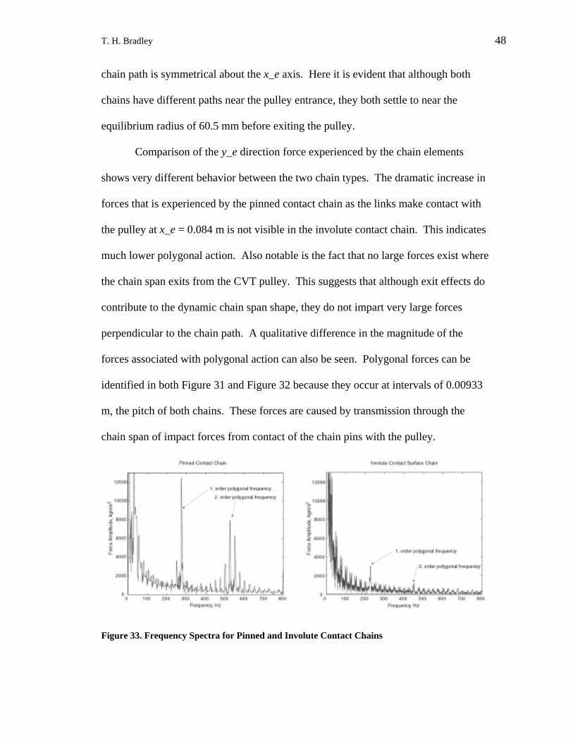
Figure 33. Frequency Spectra for Pinned and Involute Contact Chains

T. H. Bradley 49
Spectral analysis of the vibration of the chain elements in the chain span
provides for a more quantitative comparison. The spectra of the forces in the y_e
direction that are applied to the chain elements as they travel along the chain span are
presented in Figure 33. In these simulations the polygonal frequency of the involute
contact chain and the pinned contact chain are 231 Hz and 270 Hz respectively. The
difference in frequency is present because of a difference in pulley speeds, and slip
rates between the two chain designs. In both chains, both the first and second order
polygonal frequency are evident, but the magnitude of the excitations at the polygonal
frequencies is much greater for the pinned contact chain. Lower magnitudes for the
involute contact chain indicate a reduction in vibrations from polygonal action.
Figure 34. Secondary Pulley Torque Profile
The reduction in polygonal action that is present in the involute contact chain
has influences on the entire CVT system, not just the chain span. As shown in Figure
T. H. Bradley 50
34, the reduction in polygonal action more than halves the peak-to-peak torque
fluctuations that are transmitted to the CVT pulleys. This has the additional effect of
lessening the vibrations passed to other components of the drivetrain.
DYNAMIC MODELING CONCLUSIONS - The results of the dynamic model
show that there is a significant improvement in the vibration behavior of the involute
contact CVT chain when compared to the pinned contact chain. Polygonal excitation
of both the chain span and the CVT pulleys are significantly decreased, providing
further justification of the involute chain design concept. Exit effects are shown to
play a minor role in polygonal excitation of the CVT chain span
T. H. Bradley 51
CONCLUSIONS AND RECOMMENDATIONS
Static and dynamic models have been presented to analyze and simulate the
dynamics of CVT chains. The models presented show the ability to simulate
polygonal action in CVT chains and CVT variators.
The static models developed here have been used as a tool for design of the
inter-element contact surfaces. Specifically the discrete static model is used to
analyze the tradeoffs present in design of these contact surfaces. Results of the static
model can be used to predict and minimize polygonal action by solving for dh and
pin-to-pulley angle of incidence as a function of pulley radius. Results from the static
models show that, with proper design, CVT chains with involute inter-element
contact surfaces display less static mid-span displacement, smaller angle of incidence
at impact and they impact the pulley closer to tangent, when compared to pinned
contact point CVT chains. This behavior is predictive of reduced polygonal action
and the lower vibration, higher efficiency and lower sound emissions that generally
accompany that reduction.
Dynamic models were constructed to analyze polygonal action dynamically
and at the CVT system-level. A scheme of 2-D compliant contact modeling with an
explicit slip-stick friction law was developed and implemented in this model. With
the dynamic model the forces on the chain elements and on the CVT pulleys can be
predicted and compared for chains of various designs. Non-linear dynamic effects of
polygonal action can be predicted and incorporated into CVT chain design. Results
from the dynamic models show that the involute contact surface chain experiences
lower polygonal forces both at contact and at midspan. Reduced forces cause less

T. H. Bradley 52
excitation of other vibration frequencies and lower torque pulses to the pulleys and
other components of the CVT system. The large magnitude of this reduction
indicates that the involute contact surface CVT chain can significantly improve the
dynamic characteristics of CVT chains.
Future development should be centered on improvement of the dynamic chain
model. Further work is needed to improve the applicability of the model and perform
a detailed validation of the model as a whole. The implementation of the compliant
contact modeling scheme with explicit friction modeling is somewhat of a success
although stability problems demand more refinement. Simulation of various speed
and loading conditions will allow for a more detailed investigation of the dynamic
behavior of the involute chain CVT. Modeling of pulley skew and deflection will
improve the stability and validity of the simulation, especially for predicting the
behavior of the chain when in contact with the pulleys. The results of this research
are best viewed as a comparison between the involute and pinned contact chain
simulations because of incomplete model validation. Dynamic simulations are best
validated with experimental results. Experimental acoustic and dynamic testing of
CVT chains would provide a basis for further refinement of the dynamic chain
models.

T. H. Bradley 53
REFERENCES
Abadie, M. (2000). Dynamic Simulation of Rigid Bodies: Modeling of Frictional Contact. Impacts in Mechanical Systems - Analysis and Modeling. B. Brogliato. Berlin, Springer Verlag: 61-144.
Abo, K., Kobayashi, M. (2000). "Development of a new metal-belt CVT for high-torque engines." Society of Automotive Engineers Technical Paper Series, 2000-01-0829.
Ariaratnam, S. T., Asokanthan, S. F. (1987). "Dynamic stability of chain drives." Journal of Mechanisms, Transmission and Automation in Design 109: 412-418.
Avramidis, S. (1986). "A "state of the art" chain driven CVT design." Society of Automotive Engineers Technical Paper Series, 861354.
Bothwell, S. L. (1987). Investigation of Chain Dynamics with Application to Noise. Department of Mechanical and Aeronautical Engineering, University of California, Davis: 51.
Bradley, T. H., Huff, B. R., Frank, A. A. (2002). Test and Evaluation of the UC Davis Servo-Hydraulic CVT Control System and the GCI CVT Chain in a Hybrid Electric Vehicle: A Report To Nissan Motor Company, University of California, Davis: 81.
Brandsma, A., van Lith, J., Hendricks, E. (1999). Push belt CVT developments for high power applications. International Congress on Continuously Variable Power Transmission, Eindhoven, Netherlands.
Fujii, T., Kurokawa, T. (1993). "A study of a metal pushing v-belt type CVT - Part 1: Relation between transmitted torque and pulley thrust." Society of Automotive Engineers Technical Paper Series, 930666.
Gerbert, G. (1984). "Metal v-belt mechanics." ASME Paper 84-DET-227. Gerbert, G. (1996). Skew v-belt pulleys. International Conference on Continuously
Variable Power Transmission, Yokohama, Japan, Japan Society of Automotive Engineers.
Hendricks, E. (1993). "Qualitative and quantitative influence of a fully electronically controlled CVT on fuel economy and vehicle performance." Society of Automotive Engineers Technical Paper Series, 930668.
Hirano, S., Miller, A. L., Schneider, K. F. (1991). "SCVT - A state of the art electronically controlled continuously variable transmission." Society of Automotive Engineers Technical Paper Series, 910410.
Ide, T. (2000). Effect of belt loss and oil pump loss on the fuel efficiency of a vehicle with a metal v-belt CVT. FISITA World Automotive Congress, Seoul, Korea.
Johnson, K. L. (1985). Contact Mechanics. Cambridge, Cambridge University Press. Karnopp, D. (1985). "Computer simulation of stick-slip friction in mechanical
dynamic systems." Journal of Dynamic Systems, Measurement, and Control 107: 101.
Khiralla, T. F. (1976). On the Geometry of External Involute Spur Gears. North Hollywood, California, C/I Leaming.
Kluger, M. A., Long, D. M. (1999). "An overview of current automatic, manual and continuously variable transmission efficiencies and their projected future

T. H. Bradley 54
improvements." Society of Automotive Engineers Technical Paper Series, 1999-01-1259.
Kobayashi, D., Mabuchi, Y., Katoh, Y. (1998). "A study on the torque capacity of a metal pushing v-belt for CVTs." Society of Automotive Engineers Technical Paper Series, 980822.
Kraus, P. R., Kumar, V. (1997). Compliant Contact Models for Rigid Body Collisions. 1997 IEEE International Conference on Robotics and Automation, Albuquerque, New Mexico, IEEE.
Leine, R. I., Van Campen, D. H., De Kraker, A., Van Den Steen, L. (1998). "Stick-slip vibrations induced by alternate friction models." Nonlinear Dynamics 16: 41-54.
Micklem, J. D., Longmore, D. K., Burrows, C. R. (1994). "Modeling of a steel v-belt continuously variable transmission." Journal of Mechanical Engineering Science 208: 14-27.
Nikravesh, P. E. (1988). Computer-Aided Analysis of Mechanical Systems. London, Prentice-Hall.
Pfeiffer, F., Glocker, C. (1996). Multibody Dynamics with Unilateral Contacts. New York, Wiley and Sons.
Reeves, M. O. (1897). Speed Varying Mechanism. United States Patent, Reeves Pulley Company.
Sedlmayr, M., Bullinger, M., Pfeiffer, F. (2002). "Spatial dynamics of CVT chain drives." VDI Berichte 1709.
Srnik, J., Pfeiffer, F. (1994). Simulation of a CVT Chain Drive as a Multibody System with Variant Structure. The First Joint Conference of International Simulation Societies, Zurich, Switzerland.
Srnik, J., Pfeiffer, F. (1997). Dynamics of CVT chain drives: Mechanical model and verification. Design Engineering Technical Conferences, Sacramento, California.
Srnik, J., Pfeiffer, F. (1999). "Dynamics of CVT chain drives." International Journal of Vehicle Design 22(1).
Stronge, W. J. (2000). "Chain reaction from impact on coaxial multibody systems." Journal of Applied Mechanics 67: 632-635.
Stronge, W. J. (2000). Contact Problems for Elasto-Plastic Impact in Multi-body Systems. Impacts in Mechanical Systems - Analysis and Modeling. B. Brogliato. Berlin, Springer Verlag: 191-234.
Stronge, W. J. (2000). Impact Mechanics, Cambridge University Press. Takahashi, M., Kido, R., Nonaka, K., Takayama, M., Fujii, T. (1999). Design and
development of a dry hybrid belt (BANDO AVANCE) for CVT vehicles. International Congress on Continuously Variable Power Transmission CVT '99, Eindhoven, The Netherlands.
Tanaka, H., Goi, T. (1999). Traction drive of a high speed double cavity half-toroidal CVT. International Congress on Continuously Variable Power Transmission CVT '99, Eindhoven, The Netherlands.
Troedsson, I., Vedmar, L. (2001). "A dynamic analysis of the oscillations in a chain drive." Journal of Mechanical Design 123: 395-401.

T. H. Bradley 55
van Rooij, J., Frank, A. (2002). Development of a 700 Nm chain CVT. International Conference on Continuously Variable Power, Munich, Germany.
van Rooij, J. H. M. (1991). Volvo Car's new chain concept. 3rd International EAEC Conference on Vehcile Dynamics and Powertrain Engineering, Strasbourg, France.
van Rooij, J. H. M. (1993). The chain CVT. Year Book Autotechnical Trends. Arnhem, The Netherlands, Hogeschool Geluerland.
van Rooij, J. H. M., Cadee, T. P. M. (1996). Transmission chain for a cone pulley transmission. European Patent, Gear Chain Industrial B. V.
Wagner, U., Teubert, A., Endler, T. (2001). "Entwicklung von CVT-ketten fuer Pkw-anwendungen bis 400 Nm." VDI Berichte(1610).
T. H. Bradley 56
APPENDIX 1 – Discrete Static CVT Chain Model:
MATLAB M-files
inv.m
%inv.m - Discrete static cvt chain model initialization program %by: Thomas Bradley 9/17/02 clear global Rad Rb step_in tomout dt_left Q t gamma epsilon x0 = [0 %Q(2,x) = x0(1); .059 %Q(2,y) = x0(2); % y_pulley
%position of the end of A_e of link 1 -0.00933 %Q(3,x) = x0(3); .059 %Q(3,y) = x0(4); -0.00933*2 %Q(4,x) = x0(5); .059 %Q(4,y) = x0(6); -0.00933*3 %Q(5,x) = x0(7); .059 -deg2rad(20)%Q(5,y) = x0(8); -deg2rad(15)%t(1) = x0(9); % theta
%direction position of link 1 -deg2rad(11) %t(2) = x0(10); % theta
%direction position of link 2 -deg2rad(6) %t(3) = x0(11); % theta
%direction position of link 1% -deg2rad(2) %t(4) = x0(12); % theta
%direction position of link 1 -deg2rad(1) 0.2769 -0.0468 ]'; %t(5) = x0(13); % theta direction position of link 1 radius = [0.0349];%:0.002:0.078];; % !!!!!!!!!!!!!!!!!!!!! %option 1 --- works step_theta = -[ 0 0.15 0.2116 0.2463 0.2809 0.3155 0.3501 0.3847 0.4193 0.4539 0.4681 .47
T. H. Bradley 57
.48]; %option 2 step_theta = -[-0.0082 0.0264 0.0610 0.0957 0.1303 0.1649 0.1995 0.2341 0.2687]; for i = 1:length(radius) Rad = radius(i); for j = 1:length(step_theta); step_in = step_theta(j) ; options = optimset('TolFun', 1e-11, 'Display', 'iter', 'Diagnostics', 'on', 'MaxIter', 150 ); % Turn off Display [x_out,Fval,exitflag] = fsolve('involute_fxn6',x0 ,options) ; x_output(:,j) = [Q(1,:) Q(2,:) Q(3,:) Q(4,:) Q(5,:) Q(6,:) t(1:6) gamma epsilon]'; exitflag x_output; %x_out(:,j) = x'; end end x_output involute_plotter6

T. H. Bradley 58
involute_fxn6.m
function F = involute_fxn6(x0) global Rad Rb step_in tomout dt_left Q t gamma epsilon %involute_fxn6.m - Discrete static cvt chain model iteration program % called by fsolve.m %by: Thomas Bradley 9/17/02 x = 1; y = 2; Rb = 56.2327*1e-3;% % m; % !!!!!!!!!!!!!!!!!!!!! a = -1.5371; % mm; % !!!!!!!!!!!!!!!!!!!!! 0;% %Q(2,x) = x0(1); % x_pulley position of the %end of A_e of link 1 %Q(2,y) = x0(2); % y_pulley position of the %end of A_e of link 1 Q(3,x) = x0(1); % x_pulley position of the %end of A_e of link 1 Q(3,y) = x0(2); % y_pulley position of the %end of A_e of link 1 Q(4,x) = x0(3); Q(4,y) = x0(4); Q(5,x) = x0(5); Q(5,y) = x0(6); Q(6,x) = x0(7); Q(6,y) = x0(8); t(1) = x0(9); % theta direction position of link 1 t(2) = x0(10); % theta direction position of link 2 t(3) = x0(11); % theta direction position of link 1 t(4) = x0(12); % theta direction position of link 1 t(5) = x0(13); % theta direction position of link 1 t(6) = x0(14); gamma = x0(15); epsilon = x0(16); %d = x0(14); % y_pulley direction position of the %end of A_e of link 1 A_bc = [-5.5269 0]'*1e-3; % !!!!!!!!!!!!!!!!!!!!! A_b = [-3.7152 a]'*1e-3; % !!!!!!!!!!!!!!!!!!!!! B_b = [5.6149 a]'*1e-3; % !!!!!!!!!!!!!!!!!!!!! if Rb == 0 A_b = [-9.33/2 0]'*1e-3; B_b = [9.33/2 0]'*1e-3;
T. H. Bradley 59
A_bc = [-9.33/2 0]'*1e-3; end x = 1; y = 2; %I need 14 zeros in the Z vector %%%%%%%%%%%%%%%%%%%%%%%%%%%%%%%%% for element 1 %%%%%%%%%%%%%%%%%%%% %option 2 t_p = step_in; t(1) = step_in + gamma/2 + gamma - 0.04438; Q(2,x) = -Rad*sin(t_p); Q(2,y) = Rad*cos(t_p); Q(1,x) = -Rad*sin(t_p + gamma); %gamma is (-) Q(1,y) = Rad*cos(t_p + gamma); Z(1) = -t(2) + t(1) - gamma; Z(2) = -gamma - atan2(Q(2,2),Q(2,1)) + atan2(Q(1,2),Q(1,1)); %%%%%%%%%%%%%% T_1= [cos(t(1)) -sin(t(1)); sin(t(1)) cos(t(1))]; T_2= [cos(t(2)) -sin(t(2)); sin(t(2)) cos(t(2))]; T_3= [cos(t(3)) -sin(t(3)); sin(t(3)) cos(t(3))]; T_4= [cos(t(4)) -sin(t(4)); sin(t(4)) cos(t(4))]; T_5= [cos(t(5)) -sin(t(5)); sin(t(5)) cos(t(5))]; T_6= [cos(t(6)) -sin(t(6)); sin(t(6)) cos(t(6))]; %%%%%%%%%%%%%%%%%%%%%%%%%%%%%%%%% element 1 & 2 %%%%%%%%%%%%%%%%%%%% i = 2; A_ec_left = T_2*A_bc; A_e_left = T_2*A_b; B_e_left = T_2*B_b; A_e_right = T_1*A_b; B_e_right = T_1*B_b; A_ec_right = T_1*A_bc; dt_left = (t(i) - t(i+1)); x_t_left = -Rb*sin(-dt_left) + Rb*(-dt_left)*cos(-dt_left); y_t_left = Rb*cos(-dt_left) + Rb*(-dt_left)*sin(-dt_left)-Rb; if dt_left >= 0 x_t_left = 0; y_t_left = 0; end dt_right = (-t(i) + t(i-1)); x_t_right= -Rb*sin(-dt_right) + Rb*(-dt_right)*cos(-dt_right); y_t_right= Rb*cos(-dt_right) + Rb*(-dt_right)*sin(-dt_right)-Rb; if dt_right >= 0 x_t_right = 0; y_t_right = 0;
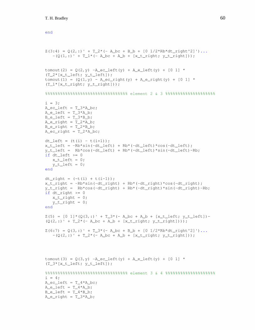
T. H. Bradley 60
end Z(3:4) = Q(2,:)' + T_2*(- A_bc + B_b + [0 1/2*Rb*dt_right^2]')... -(Q(1,:)' + T_1*(- A_bc + A_b + [x_t_right; y_t_right])); tomout(2) = Q(2,y) -A_ec_left(y) + A_e_left(y) + [0 1] * (T_2*[x_t_left; y_t_left]); tomout(1) = (Q(1,y) - A_ec_right(y) + A_e_right(y) + [0 1] * (T_1*[x_t_right; y_t_right])); %%%%%%%%%%%%%%%%%%%%%%%%%%%%%%%%% element 2 & 3 %%%%%%%%%%%%%%%%%%%% i = 3; A_ec_left = T_3*A_bc; A_e_left = T_3*A_b; B_e_left = T_3*B_b; A_e_right = T_2*A_b; B_e_right = T_2*B_b; A_ec_right = T_2*A_bc; dt_left = (t(i) - t(i+1)); x_t_left = -Rb*sin(-dt_left) + Rb*(-dt_left)*cos(-dt_left); y_t_left = Rb*cos(-dt_left) + Rb*(-dt_left)*sin(-dt_left)-Rb; if dt_left >= 0 x_t_left = 0; y_t_left = 0; end dt_right = (-t(i) + t(i-1)); x_t_right = -Rb*sin(-dt_right) + Rb*(-dt_right)*cos(-dt_right); y_t_right = Rb*cos(-dt_right) + Rb*(-dt_right)*sin(-dt_right)-Rb; if dt_right >= 0 x_t_right = 0; y_t_right = 0; end Z(5) = [0 1]*(Q(3,:)' + T_3*(- A_bc + A_b + [x_t_left; y_t_left])-(Q(2,:)' + T_2*(- A_bc + A_b + [x_t_right; y_t_right]))); Z(6:7) = Q(3,:)' + T_3*(- A_bc + B_b + [0 1/2*Rb*dt_right^2]')... -(Q(2,:)' + T_2*(- A_bc + A_b + [x_t_right; y_t_right])); tomout(3) = Q(3,y) -A_ec_left(y) + A_e_left(y) + [0 1] * (T_3*[x_t_left; y_t_left]); %%%%%%%%%%%%%%%%%%%%%%%%%%%%%%%%% element 3 & 4 %%%%%%%%%%%%%%%%%%%% i = 4; A_ec_left = T_4*A_bc; A_e_left = T_4*A_b; B_e_left = T_4*B_b; A_e_right = T_3*A_b;
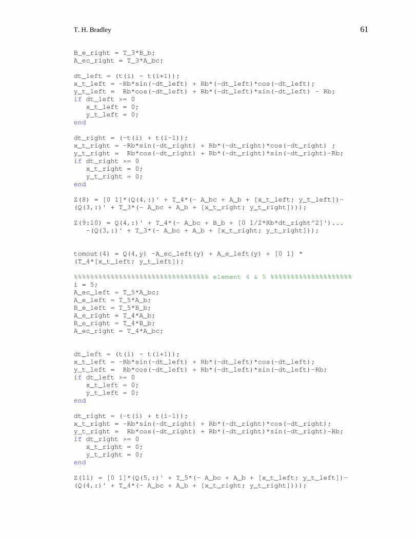
T. H. Bradley 61
B_e_right = T_3*B_b; A_ec_right = T_3*A_bc; dt_left = (t(i) - t(i+1)); x_t_left = -Rb*sin(-dt_left) + Rb*(-dt_left)*cos(-dt_left); y_t_left = Rb*cos(-dt_left) + Rb*(-dt_left)*sin(-dt_left) - Rb; if dt_left >= 0 x_t_left = 0; y_t_left = 0; end dt_right = (-t(i) + t(i-1)); x_t_right = -Rb*sin(-dt_right) + Rb*(-dt_right)*cos(-dt_right) ; y_t_right = Rb*cos(-dt_right) + Rb*(-dt_right)*sin(-dt_right)-Rb; if dt_right >= 0 x_t_right = 0; y_t_right = 0; end Z(8) = [0 1]*(Q(4,:)' + T_4*(- A_bc + A_b + [x_t_left; y_t_left])-(Q(3,:)' + T_3*(- A_bc + A_b + [x_t_right; y_t_right]))); Z(9:10) = Q(4,:)' + T_4*(- A_bc + B_b + [0 1/2*Rb*dt_right^2]')... -(Q(3,:)' + T_3*(- A_bc + A_b + [x_t_right; y_t_right])); tomout(4) = Q(4,y) -A_ec_left(y) + A_e_left(y) + [0 1] * (T_4*[x_t_left; y_t_left]); %%%%%%%%%%%%%%%%%%%%%%%%%%%%%%%%% element 4 & 5 %%%%%%%%%%%%%%%%%%%% i = 5; A_ec_left = T_5*A_bc; A_e_left = T_5*A_b; B_e_left = T_5*B_b; A_e_right = T_4*A_b; B_e_right = T_4*B_b; A_ec_right = T_4*A_bc; dt_left = (t(i) - t(i+1)); x_t_left = -Rb*sin(-dt_left) + Rb*(-dt_left)*cos(-dt_left); y_t_left = Rb*cos(-dt_left) + Rb*(-dt_left)*sin(-dt_left)-Rb; if dt_left >= 0 x_t_left = 0; y_t_left = 0; end dt_right = (-t(i) + t(i-1)); x_t_right = -Rb*sin(-dt_right) + Rb*(-dt_right)*cos(-dt_right); y_t_right = Rb*cos(-dt_right) + Rb*(-dt_right)*sin(-dt_right)-Rb; if dt_right >= 0 x_t_right = 0; y_t_right = 0; end Z(11) = [0 1]*(Q(5,:)' + T_5*(- A_bc + A_b + [x_t_left; y_t_left])-(Q(4,:)' + T_4*(- A_bc + A_b + [x_t_right; y_t_right])));

T. H. Bradley 62
Z(12:13) = Q(5,:)' + T_5*(- A_bc + B_b + [0 1/2*Rb*dt_right^2]')... -(Q(4,:)' + T_4*(- A_bc + A_b + [x_t_right; y_t_right])); tomout(5) = Q(5,y) -A_ec_left(y) + A_e_left(y) + [0 1] * (T_5*[x_t_left; y_t_left]); %%%%%%%%%%%%%%%%%%%%%%%%%%%%%%%%% element 5 & 6 %%%%%%%%%%%%%%%%%%%% i = 6; A_ec_left = T_6*A_bc; A_e_left = T_6*A_b; B_e_left = T_6*B_b; A_e_right = T_5*A_b; B_e_right = T_5*B_b; A_ec_right = T_5*A_bc; t(7) = 0; dt_left = (t(i) - t(i+1)); x_t_left = -Rb*sin(-dt_left) + Rb*(-dt_left)*cos(-dt_left); y_t_left = Rb*cos(-dt_left) + Rb*(-dt_left)*sin(-dt_left)-Rb; if dt_left >= 0 x_t_left = 0; y_t_left = 0; end dt_right = (-t(i) + t(i-1)); x_t_right = -Rb*sin(-dt_right) + Rb*(-dt_right)*cos(-dt_right); y_t_right = Rb*cos(-dt_right) + Rb*(-dt_right)*sin(-dt_right)-Rb; if dt_right >= 0 x_t_right = 0; y_t_right = 0; end Z(14) = [0 1]*(Q(6,:)' + T_6*(- A_bc + A_b + [x_t_left; y_t_left])-(Q(5,:)' + T_5*(- A_bc + A_b + [x_t_right; y_t_right]))); Z(15:16) = Q(6,:)' + T_6*(- A_bc + B_b + [0 1/2*Rb*dt_right^2]')... -(Q(5,:)' + T_5*(- A_bc + A_b + [x_t_right; y_t_right])); tomout(6) = Q(6,y) -A_ec_left(y) + A_e_left(y) + [0 1] * (T_6*[x_t_left; y_t_left]); %%%%%%%%%%%%%%%%%%%%%%%%%%%%%%%%% F = Z';

T. H. Bradley 63
APPENDIX 2 – Dynamic CVT Chain Model:
MATLAB M-files
chain_init_v13f.m
% chain_init.m % This m-file determines the initial locations of the links at a 1:1 % ratio, and initializes the Runge Kutta solver % Thomas Bradley 7/8/01 disp('Running - gci_init_v13f.m') for n_times = 1:1 format compact tic clear global c2c l_link n_links A_b B_b r K_b C_b M center1 center2 global pulley_beta contact_flag force_comp w_p U C_mat A_mat global A_e B_e h step contact_flag_out dYdt_pre t_end K_e C_e R global F_clamp K_link w_link z0 F_t F_n e_v_contactt global mu_s mu_d e_F_l e_t_l e_n_l r_pulley dist_c e_r_sigp e_n_p global m_out e_v_contactn m e_t_p U_out dYdt_1 Z global I_link t_end_last J_pulley Z_out Y_test contact_flag2 cf_out global pulley_i A_ec Z_last A_bc B_bc e_v_contact_tangential global e_v_pullc plotting = 0; disp('Link Position Initialization...') disp('Overall Length Error, mm') start_over = 0%<------------------------------- this is the restart if start_over == 0 load chain_output21_29 size_buff = size(Y_out); Y0 = Y_out(size_buff(1),:); n_links = 75; % # of links r = 59.3 % r is the 1:1 radius of the chain; (mm) elseif start_over == 2 done = 0; c2c = 167.99e-3; % Nissan 2L CVT center to center pulley %distance (m) l_link = 9.33/1000; % GCI link length (m) r = 59.3e-3 ; % r is the 1:1 radius of the chain; (mm) n_links = floor(2*pi*r/.00925); angle = [0:2*pi/n_links:(2*pi-2*pi/n_links)]; x_init = sin(angle) * r; y_init = cos(angle) * r; theta_init = -angle+2*pi; for i = 1:length(theta_init)

T. H. Bradley 64
if theta_init(i) <= -pi; theta_init(i) = theta_init(i) + 2*pi; end end x_dot_init = zeros(1,n_links); y_dot_init = zeros(1,n_links); theta_dot_init = zeros(1,n_links); Y0 = [(x_init-c2c/2) y_init theta_init x_dot_init y_dot_init theta_dot_init 0 0.001 0 0];
load gci_output6_5 size_buff = size(Y_out); Y0 = Y_out(size_buff(1),:); clear Y_out elseif start_over == 1 c2c = 167.99; % Nissan 2L CVT center to center pulley % distance (mm) l_link = 9.29 % GCI link length (mm) est. n_links = 75; % # of links r = 56; % r is the 1:1 radius of the chain; (mm) done = 0; while done == 0 x = zeros(n_links,2); % vector of link positions, has the % form [x y] (mm) x(1,:) = [-c2c/2 r]; % this establishes the position of % the 1st pin (mm) top = 1; % this flag goes off when the % program is assigning the % position of the links on the % bottom of the chain through = 0; thru = 0; for i=2:76 if top == 1 % corresponds to section 1 and 2 of the chain. p9 x(i,:) = x(i-1,:)+[l_link 0]; if x(i,1) >= c2c/2 % corresponds to section 2 of the chain. p9 xbuff = zeros(1,2); xbuff(1,:) = x(i-1,:) - [c2c/2 0]; % xbuff holds the position of the previous link % where the pulley is centered at the origin [x2,y2] = solve('l_link = sqrt((xbuff(1,1) - x2)^2+(xbuff(1,2)-y2)^2)','r^2 = x2^2+y2^2'); % solves the equation for where the pulley % diameter and the link length interesect x(i,1) = max(eval(x2))+c2c/2 ; % going clockwise the rightmost x % coord and the lowest % y coord should be taken x(i,2) = min(eval(y2)); if x(i,2) <=0 buff_dude = (eval(x2))+c2c/2; x(i,1) = buff_dude(2); % when you round the corner the

T. H. Bradley 65
% leftmost x coord end end if (x(i,2)-x(i-1,2)) > 0 top = 0; % if the link begins to move % upwards around the circle % then the not_top regime has been % reached end end if (top == 0) xbuff = zeros(1,2); xbuff(1,:) = x(i-1,:) - [c2c/2 0]; [x2] = solve('l_link = sqrt((xbuff(1,1) - x2)^2+(xbuff(1,2)-r)^2)'); x(i,1) = min(eval(x2))+c2c/2 ; end if and((x(i,2)-x(i-1,2)) >= 0, top == 0) % if it is not in the top regime % and link is going down or flat x(i,:) = x(i-1,:)-[l_link 0]; end if and(top == 0,x(i,1) <= -c2c/2) % if it is not in the top regime % and the link is past the flat % section this corresponds to % section 4 of the chain. p9 xbuff = zeros(1,2); xbuff(1,:) = x(i-1,:) + [c2c/2 0]; [x2,y2] = solve('l_link = sqrt((xbuff(1,1) - x2)^2+(xbuff(1,2)-y2)^2)','r^2 = x2^2+y2^2'); x(i,1) = min(eval(x2))-c2c/2; if through == 1 buff = (eval(y2)); x(i,2) = buff(1); else buff = (eval(y2)); x(i,2) = buff(2); through = 1; end if x(i,2) >=0 if thru == 1 x(i,1) = max(eval(x2))-c2c/2 ; else x(i,1) = min(eval(x2))-c2c/2 ; thru = 1; end end end end (x(i) - x(1)) if abs(x(i) - x(1)) <= .0001

T. H. Bradley 66
done = 1; else r = r+(x(i) - x(1))/2/pi*1 % refine the radius at which % the chain rides on the pulley end end X = x(1:n_links,:)/1000; % output the position matrix for % the chain link CGs (m) r = r/1000 ; % pulley radius at which the % chain rides (m) if plotting == 1 figure plot(X(:,1),X(:,2),'-') axis equal grid else disp('plotting off') end %%%%%%%%%%%%%%%%%%%%%%%%%%%%%%%%%%%%%%%%%%%%%%%%%%%%%%%%%%% disp('Link Direction and Velocity Initialization...') for i=1:length(X) a = i-1; b = i; c = i+1; if i == 1 a = n_links; % index of m-1 b = 1; % index of m c = 2; % index of m+1 end if i == n_links a = n_links-1; % index of m-1 b = n_links; % index of m c = 1; % index of m+1 end dx = x(c,1)- x(a,1); dy = x(c,2) - x(a,2); theta(i) = atan2(dy,dx); theta_vect(i,1:2) = 1/sqrt(dx^2+dy^2)*[dx dy]; speed = 100*2*pi/60*r; end theta(56) = -theta(56); %initialize the Y vector for DOFs of the system Y(1:length(X)) = X(:,1); % link x position (m) Y((length(X)+1):(2*length(X))) = X(:,2); % link y position (m) Y((2*length(X)+1):(3*length(X))) = theta-2*pi;
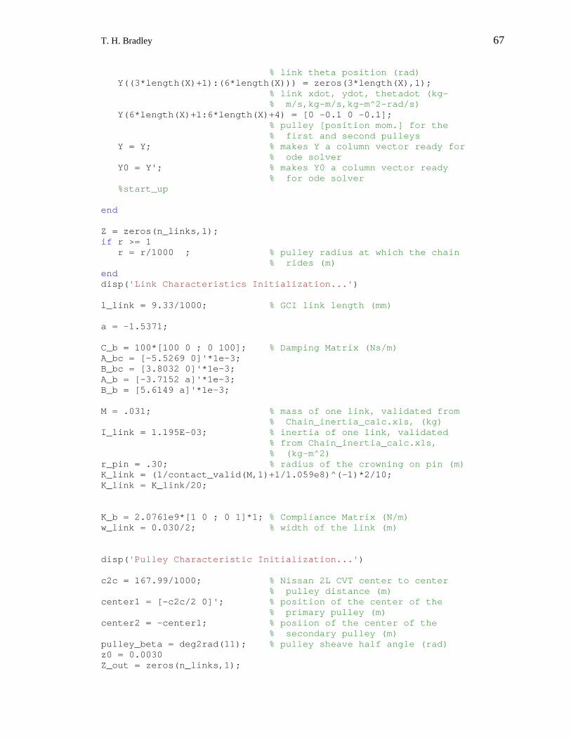
T. H. Bradley 67
% link theta position (rad) Y((3*length(X)+1):(6*length(X))) = zeros(3*length(X),1); % link xdot, ydot, thetadot (kg- % m/s,kg-m/s,kg-m^2-rad/s) Y(6*length(X)+1:6*length(X)+4) = [0 -0.1 0 -0.1]; % pulley [position mom.] for the % first and second pulleys Y = Y; % makes Y a column vector ready for % ode solver Y0 = Y'; % makes Y0 a column vector ready % for ode solver %start_up end Z = zeros(n_links,1); if r >= 1 r = r/1000 ; % pulley radius at which the chain % rides (m) end disp('Link Characteristics Initialization...') l_link = 9.33/1000; % GCI link length (mm) a = -1.5371; C_b = 100*[100 0 ; 0 100]; % Damping Matrix (Ns/m) A_bc = [-5.5269 0]'*1e-3; B_bc = [3.8032 0]'*1e-3; A_b = [-3.7152 a]'*1e-3; B_b = [5.6149 a]'*1e-3; M = .031; % mass of one link, validated from % Chain_inertia_calc.xls, (kg) I_link = 1.195E-03; % inertia of one link, validated % from Chain_inertia_calc.xls, % (kg-m^2) r_pin = .30; % radius of the crowning on pin (m) K_link = (1/contact_valid(M,1)+1/1.059e8)^(-1)*2/10; K_link = K_link/20; K_b = 2.0761e9*[1 0 ; 0 1]*1; % Compliance Matrix (N/m) w_link = 0.030/2; % width of the link (m) disp('Pulley Characteristic Initialization...') c2c = 167.99/1000; % Nissan 2L CVT center to center % pulley distance (m) center1 = [-c2c/2 0]'; % position of the center of the % primary pulley (m) center2 = -center1; % posiion of the center of the % secondary pulley (m) pulley_beta = deg2rad(11); % pulley sheave half angle (rad) z0 = 0.0030 Z_out = zeros(n_links,1);

T. H. Bradley 68
F_clamp = 10; % total compressive force from each % pulley (N) w_p = [0 0 0]'; % pulley angular velocity, negative is % CW (rad/sec) mu_s = 0.12; % coefficient of static friction mu_d = .09; % coefficient of dynamic friction J_pulley = 0.028; % rotational moment of inertia for the % pulley (kg-m^2) step = 0; %h = waitbar(0,'Tom this is your thesis talking. Your ass is mine!!!'); t_end = 1e-2 tspan = [0:t_end/500:t_end];%[0 t_end];% size(Y0) disp('Done - gci_init_v13f.m') %%%%%%%%%%%%% disp('Running - gci_ode_v13f.m') Y = Y0'; step = 0; output_step = 1; done = 0; time = 0; dh = 5e-6; while ~done step = step+1 ; dYdt1 = gci_ode_v13f(time,Y,Y0); dYdt2 = gci_ode_v13f(time+dh/2, Y+dh/2*dYdt1, Y0); dYdt3 = gci_ode_v13f(time+dh/2, Y+dh/2*dYdt2, Y0); dYdt4 = gci_ode_v13f(time+dh, Y+dh*dYdt3, Y0); Y_next = Y + 1/6*(dYdt1 + 2*dYdt2 + 2*dYdt3 + dYdt4)*dh; Y_out(step,:) = Y'; if step == 1 time_prev = 0; else time_prev = time(step-1); end time(step) = time_prev+dh;
if time(step) >= t_end done = 1; end Y = Y_next; time(length(time)) end toc toc save chain_output21_30 end sound((sin((5*[1:10000]))))

T. H. Bradley 69
chain_ode_v13f.m
function dYdt = chain_ode_v13f(t,Y,Y0) %This m-file determines the system of equations and outputs dY/dt. %Thomas Bradley 7/8/01 global c2c l_link n_links A_b B_b r K_b C_b M center1 center2 global pulley_beta contact_flag force_comp w_p U C_mat A_mat global A_e B_e h step contact_flag_out dYdt_pre t_end K_e C_e R global F_clamp K_link w_link z0 F_t F_n e_v_contactt global mu_s mu_d e_F_l e_t_l e_n_l r_pulley dist_c e_r_sigp e_n_p global m_out e_v_contactn m e_t_p U_out dYdt_1 Z global I_link t_end_last J_pulley Z_out Y_test contact_flag2 cf_out global pulley_i A_ec Z_last A_bc B_bc e_v_pullc global e_v_contact_tangential % define the System Dynamics Matrix A_mat A_mat = sparse(zeros(6*n_links+4)); % define the Non-linearities Dynamics Matrix C-mat C_mat = sparse(zeros(6*n_links+4)); U = sparse(zeros(6*n_links+4,1)); contact_flag = zeros(n_links,1); qy_i = n_links; % index to get the y values in Y qtheta_i = 2*n_links; % index to get the theta values in Y px_i = 3*n_links; % index to get the x_dot values % in Y, and the x_ddot solution % row in A_mat py_i = 4*n_links; % index to get the y_dot values % in Y ptheta_i = 5*n_links; % index to get the theta_dot % values in Y pulley_i = 6*n_links; %%%%%%%%%%%%%%%%%%%%%%%%%%%%%%%%%%%%%%%%%%%%%%%%%%%%%%%%%%%%%%%%%%%% U(pulley_i+2) = -100; % Primary Pulley input torque (Nm) U(pulley_i+4) = -100; % Secondary Pulley output torque (Nm) %%%%%%%%%%%%%%%%%%%%%%%%%%%%%%%%%%%%%%%%%%%%%%%%%%%%%%%%%%%%%%%%%%%% K_e = K_b(1,1); C_e1 = C_b(1,1); % this is the xy damping constant C_e2 = C_b(1,1)/100; % this is the damping constant for % theta C_e3 = C_b(1,1)/10; % this is the damping constant for % theta also for m = 1:n_links; a = m-1; b = m; c = m+1; if m == 1 a = n_links; % index of m-1 b = 1; % index of m c = 2; % index of m+1 end if m == n_links
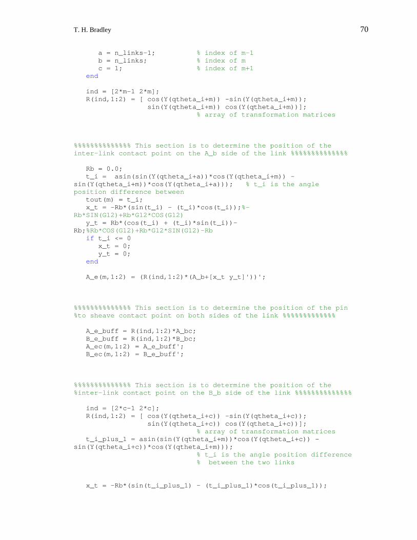
T. H. Bradley 70
a = n_links-1; % index of m-1 b = n_links; % index of m c = 1; % index of m+1 end ind = [2*m-1 2*m]; R(ind,1:2) = [ cos(Y(qtheta_i+m)) -sin(Y(qtheta_i+m)); sin(Y(qtheta_i+m)) cos(Y(qtheta_i+m))]; % array of transformation matrices %%%%%%%%%%%%%% This section is to determine the position of the inter-link contact point on the A_b side of the link %%%%%%%%%%%%%% Rb = 0.0; t_i = asin(sin(Y(qtheta_i+a))*cos(Y(qtheta_i+m)) - sin(Y(qtheta_i+m))*cos(Y(qtheta_i+a))); % t_i is the angle position difference between tout(m) = t_i; x_t = -Rb*(sin(t_i) - (t_i)*cos(t_i));%-Rb*SIN(G12)+Rb*G12*COS(G12) y_t = Rb*(cos(t_i) + (t_i)*sin(t_i))-Rb;%Rb*COS(G12)+Rb*G12*SIN(G12)-Rb if t_i <= 0 x_t = 0; y_t = 0; end A_e(m,1:2) = (R(ind,1:2)*(A_b+[x_t y_t]'))'; %%%%%%%%%%%%%% This section is to determine the position of the pin %to sheave contact point on both sides of the link %%%%%%%%%%%%% A_e_buff = R(ind,1:2)*A_bc; B_e_buff = R(ind,1:2)*B_bc; A_ec(m,1:2) = A_e_buff'; B_ec(m,1:2) = B_e_buff'; %%%%%%%%%%%%%% This section is to determine the position of the %inter-link contact point on the B_b side of the link %%%%%%%%%%%%%% ind = [2*c-1 2*c]; R(ind,1:2) = [ cos(Y(qtheta_i+c)) -sin(Y(qtheta_i+c)); sin(Y(qtheta_i+c)) cos(Y(qtheta_i+c))]; % array of transformation matrices t_i_plus_1 = asin(sin(Y(qtheta_i+m))*cos(Y(qtheta_i+c)) - sin(Y(qtheta_i+c))*cos(Y(qtheta_i+m))); % t_i is the angle position difference % between the two links x_t = -Rb*(sin(t_i_plus_1) - (t_i_plus_1)*cos(t_i_plus_1));

T. H. Bradley 71
% equation of the involute y_t = Rb*(cos(t_i_plus_1) + (t_i_plus_1)*sin(t_i_plus_1))-Rb; % equation of the involute if t_i_plus_1 <= 0 %keeps the involute from going backwards x_t = 0; y_t = 0; end B_e(m,1:2) = (R([2*m-1 2*m],1:2)*(B_b + 0.5*Rb*t_i_plus_1^2))' ; % coord x-formation of B_b plus the involute arc length end for pulley = 1:2 % integrate to get pulley position from momentum A_mat(pulley_i+2*pulley-1,pulley_i+2*pulley) = 1/J_pulley; end for m = 1:n_links a = m-1; b = m; c = m+1; if m == 1 a = n_links; % index of m-1 b = 1; % index of m c = 2; % index of m+1 end if m == n_links a = n_links-1; % index of m-1 b = n_links; % index of m c = 1; % index of m+1 end % The 1st portion of A_mat corresponds to % x_dot = A_mat x + B_mat u where x_dot = x_dot A_mat(m,px_i+m) = 1/M; % The next portion of A_mat corresponds to % y_dot = A_mat x+B_mat u where y_dot = y_dot A_mat(qy_i+m,py_i+m) = 1/M; % The next portion of A_mat corresponds to % theta_dot = A_mat x+B_mat u where % theta_dot = theta_dot A_mat(qtheta_i+m,ptheta_i+m) = 1/I_link; % The next portion of A_mat corresponds to % x_ddot = A_mat x+B_mat u where x_ddot = sum F % assign the values to the A_mat that define px A_mat(px_i+m,a) = K_e; A_mat(px_i+m,b) = -2*K_e; A_mat(px_i+m,c) = K_e; C_mat(px_i+m,a) = K_e*B_e(a,1); C_mat(px_i+m,b) = -K_e*(B_e(b,1)+A_e(b,1)); C_mat(px_i+m,c) = K_e*A_e(c,1); % assign the values to the A_mat that define py A_mat(py_i+m,qy_i+a) = K_e; A_mat(py_i+m,qy_i+b) = -2*K_e; A_mat(py_i+m,qy_i+c) = K_e;

T. H. Bradley 72
C_mat(py_i+m,qy_i+a) = K_e*B_e(a,2); C_mat(py_i+m,qy_i+b) = -K_e*(B_e(b,2)+A_e(b,2)); C_mat(py_i+m,qy_i+c) = K_e*A_e(c,2); % assign the values to the A_mat that define ptheta A_mat(ptheta_i+m,a) = -K_e * A_e(b,2); A_mat(ptheta_i+m,b) = K_e * A_e(b,2) + K_e * B_e(b,2) ; A_mat(ptheta_i+m,c) = -K_e * B_e(b,2); C_mat(ptheta_i+m,a) = -K_e * A_e(b,2) * B_e(a,1); C_mat(ptheta_i+m,b) = 0; C_mat(ptheta_i+m,c) = -K_e * A_e(c,1) * B_e(b,2); A_mat(ptheta_i+m,qy_i+a) = K_e * A_e(b,1); A_mat(ptheta_i+m,qy_i+b) = -K_e * A_e(b,1) - K_e * B_e(b,1); A_mat(ptheta_i+m,qy_i+c) = K_e * B_e(b,1); C_mat(ptheta_i+m,qy_i+a) = K_e * B_e(a,2) * A_e(b,1); C_mat(ptheta_i+m,qy_i+b) = 0; C_mat(ptheta_i+m,qy_i+c) = K_e * B_e(b,1) * A_e(c,2); % assign the values to the A_mat that define px damping terms A_mat(px_i+m,px_i+a) = C_e1; A_mat(px_i+m,px_i+b) = -2*C_e1; A_mat(px_i+m,px_i+c) = C_e1; A_mat(px_i+m,ptheta_i+a) = C_e1 * B_e(a,2); A_mat(px_i+m,ptheta_i+b) = -C_e1 * (B_e(b,2) + A_e(b,2)); A_mat(px_i+m,ptheta_i+c) = C_e1 * A_e(c,2); % assign the values to the A_mat that define py A_mat(py_i+m,py_i+a) = C_e1; A_mat(py_i+m,py_i+b) = -2*C_e1; A_mat(py_i+m,py_i+c) = C_e1; A_mat(py_i+m,ptheta_i+a) = C_e1 * B_e(a,1); A_mat(py_i+m,ptheta_i+b) = -C_e1 * (B_e(b,1) + A_e(b,1)); A_mat(py_i+m,ptheta_i+c) = C_e1 * A_e(c,1); % assign the values to the A_mat that define the theta % direction damping A_mat(ptheta_i+m,px_i+a) = -C_e2/M* A_e(b,2); A_mat(ptheta_i+m,px_i+b) = C_e2/M* A_e(b,2) + C_e2/M* B_e(b,2); A_mat(ptheta_i+m,px_i+c) = -C_e2/M* B_e(b,2); A_mat(ptheta_i+m,py_i+a) = C_e2/M* A_e(b,1); A_mat(ptheta_i+m,py_i+b) = -C_e2/M* A_e(b,1) - C_e2/M* B_e(b,1); A_mat(ptheta_i+m,py_i+c) = C_e2/M* B_e(b,1); A_mat(ptheta_i+m,ptheta_i+a) = C_e3/I_link* B_e(a,1)*A_e(b,1) + C_e3/I_link* B_e(a,2)*A_e(b,2);

T. H. Bradley 73
A_mat(ptheta_i+m,ptheta_i+b) = -C_e3/I_link* A_e(b,1)*A_e(b,1) - C_e3/I_link* B_e(b,1)*B_e(b,1) - C_e3/I_link* A_e(b,2)*A_e(b,2) - C_e3/I_link * B_e(b,2)*B_e(b,2) ; A_mat(ptheta_i+m,ptheta_i+c) = C_e3/I_link* A_e(c,1)*B_e(b,1) + C_e3/I_link* A_e(c,2)*B_e(b,2); end dYdt_1 = A_mat*Y+C_mat*ones(size(U)); %%%%%%%%%%%%%%%%%%%%%%%%%%%% Contact Mechanics %%%%%%%%%%%%%%%%%%%%% theta_l = -pulley_beta; % This makes the contact always happen at the the center of the pin % This does not capture the roundness of the pin Y_test = Y; for m = 1:n_links if Y(m) >= 0 theta_p = atan2(-center2(2,1) + (Y(qy_i+m) + A_ec(m,2)),-center2(1,1) + (Y(m) + A_ec(m,1))) ; e_r_p = [center2(1,1) center2(2,1) 0]'; % position vector of the pulley center (m) cf = 2; else theta_p = atan2((-center1(2,1) + (Y(qy_i+m) + A_ec(m,2))),(-center1(1,1) + (Y(m) + A_ec(m,1)))) ; e_r_p = [center1(1,1) center1(2,1) 0]'; % position vector of the pulley center (m) cf = 1; end r_pulley = sqrt((-e_r_p(2,1) + (Y(qy_i+m) + A_ec(m,2)))^2 + (-e_r_p(1,1) + (Y(m) + A_ec(m,1)))^2); e_r_sigp = [cos(theta_p) sin(theta_p) tan(pulley_beta)]'*r_pulley + [0 0 z0]' ; % position vector of the contour of the % pulley in earth coords from the center of % the pulley e_n_p3 = [cos(theta_p)*sin(pulley_beta) sin(theta_p)*sin(pulley_beta) -cos(pulley_beta)]'; % pulley normal vector in earth coords (1) e_t_p2 = [-sin(theta_p) cos(theta_p) 0]'; % pulley tangent vector in earth coords (2) e_t_p1 = cross(e_t_p2,e_n_p3); % pulley tangent vector in earth coords % facing up at theta = 0 (3) e_r_sigl = [ 0 0 (w_link)]' + [A_ec(m,1) A_ec(m,2) 0]'; % position vector of the contour of the pin % in earth coords e_r_dist = e_r_sigl + [Y(m) Y(qy_i+m) 0]' - e_r_sigp - e_r_p; % distance vector between the pulley contact % and the pin from the pulley to the pin if norm(e_r_dist) == 0 contact_bool = 1; else contact_bool = ((e_r_dist/norm(e_r_dist))'*e_n_p3 <= 0); end
T. H. Bradley 74
if contact_bool == 1 e_v_pullc=cross(1/J_pulley*[0 0 Y(pulley_i+2*cf)]',e_r_sigp) ; contact_flag(m) = cf; e_v_linkc = 1/M*[Y(px_i+m) Y(py_i+m) 0]' + cross(1/I_link*[0 0 Y(ptheta_i+m)]',e_r_sigl); % velocity in earth coords of the link % contact point. (v_link = v_cg + w x % r_contact_point) e_v_contact = e_v_pullc - e_v_linkc; % velocity of the pulley in the earth coords % of the pulley from the pin e_v_contact1 = e_v_contact'*e_t_p1; e_v_contact2 = e_v_contact'*e_t_p2; e_v_contact3 = e_v_contact'*e_n_p3; % mag of relative velocity in each direction e_v_contact_tangential = sqrt(e_v_contact1^2 + e_v_contact2^2); % mag of relative velocity in the plane of % the pin contact Z(m) = (r_pulley*tan(pulley_beta)+z0-w_link); if Z(m) >= 0 Z(m) = 0; end e_F_l = [dYdt_1(px_i+m) dYdt_1(py_i+m) (+K_link*abs(Z(m)))]'+ e_n_p3*K_link*abs(Z(m))^(1)/cos(pulley_beta); % sum of the external force on the link F_n3 = +K_link*abs(Z(m))^(1)/cos(pulley_beta); F_t2 = e_F_l'*e_t_p2; F_t1 = e_F_l'*e_t_p1; will_it_stick = 3;%<--------------------change this friction if will_it_stick == 0 mu = 0.15*(1-exp(-e_v_contact_tangential/1)) ; F_t = mu*F_n3*(e_v_contact2*e_t_p2 + e_v_contact1*e_t_p1)/e_v_contact_tangential; F_contact = F_n3 * e_n_p3 + F_t; U(px_i+m,1) = -F_contact(1,1); U(py_i+m,1) = F_contact(2,1); U(ptheta_i+m,1) = -F_contact(1,1)*A_ec(m,2) + F_contact(2,1)*A_ec(m,1); elseif will_it_stick == 2 %Leine et al friction epsilon = 1e10; %friction steepness factor, Leine et. al. mu = 0.15*2/pi*atan(abs(e_v_contact_tangential)*epsilon) /(1+3*abs(e_v_contact_tangential)); if and(mu <= 0.06, abs(e_v_contact_tangential) >= 0.1) mu = 0.06; end F_t = (mu*F_n3)*(e_v_contact2*e_t_p2 + e_v_contact1*e_t_p1)/sqrt(e_v_contact2^2 + e_v_contact1^2); % Friction force opposite in direction of % the movement of the pulley relative to % the pin F_contact = F_n3 * e_n_p3 + F_t;
T. H. Bradley 75
U(px_i+m,1) = F_contact(1,1); U(py_i+m,1) = F_contact(2,1); else % Karnopp/Leine Friction Model mu = 0.2; if abs(e_v_contact_tangential) >= .1; % slip F_t = mu*F_n3*(e_v_contact2*e_t_p2 + e_v_contact1*e_t_p1)/sqrt(e_v_contact2^2 + e_v_contact1^2); F_contact = F_n3 * e_n_p3 + F_t; U(px_i+m,1) = F_contact(1,1); U(py_i+m,1) = F_contact(2,1); elseif(sqrt((F_t2^2+F_t1^2)) > mu*F_n3*1.05) % stick to slip transition F_t = (sqrt((F_t2^2+F_t1^2)) - mu*F_n3) * (e_t_p2*sign(F_t2) + e_t_p1*sign(F_t1))/sqrt(2); % mag(external force) - mag(friction) F_contact = F_t + F_n3 * e_n_p3; U(px_i+m,1) = F_contact(1,1); U(py_i+m,1) = F_contact(2,1); %U(ptheta_i+m,1) = F_contact(2,1)*A_ec(m,1) - F_contact(1,1)*A_ec(m,2); else % stick F_t = e_v_contact_tangential*sqrt(1000/M) *(e_v_contact2*e_t_p2 + e_v_contact1*e_t_p1)/e_v_contact_tangential; % mag * (-)direction of motion F_contact = F_n3 * e_n_p3 + F_t; % this is the 3-D vector of contact forces % at the point of contact U(px_i+m,1) = F_contact(1,1); U(py_i+m,1) = F_contact(2,1); %U(ptheta_i+m,1) = F_contact(2,1)*A_ec(m,1) - F_contact(1,1)*A_ec(m,2); end end U(pulley_i+2*cf) = U(pulley_i+2*cf) - F_t'*e_t_p2*r_pulley; % Pulley reaction torque (Nm) else F_contact = [0 0 0]'*1e3; Z(m) = 0;% end end dYdt = A_mat*Y+C_mat*ones(size(U))+U; %return to gci_init program;

T. H. Bradley 76
APPENDIX 3 – Linear Elastic Link Compliance
Calculation: MATLAB M-file
link_comp.m
clear close all %~~~~~~~~~~~~~~~~~~~~~~~~~~~~~~~~~~~~~~~~~~~~~~~~~~~~~~~~~~~~~~~~~~~~~~~~% % PIN BENDING COMPLIANCE %~~~~~~~~~~~~~~~~~~~~~~~~~~~~~~~~~~~~~~~~~~~~~~~~~~~~~~~~~~~~~~~~~~~~~~~~% E = 2.068427e+011; B = .003; A = .010; I = pi*B*A^3/4; L = 30e-3; A_1 = [0:8]*3*.00084 + 0.00492; A_2 = [-10 -8 -4 -2 2 4 8 10]*.00084 + .015; A_tot = [A_1 A_2]; for load = 1:10 W = 35e3/10 * load / length(A_1); for j = 1:length(A_tot) x = [0:.0001:.030]'; a = A_tot(j); if j > length(A_1) W = -35e3/10 * load / length(A_2); end for i = 1:length(x) if x(i) >= a F_v(i) = W * (x(i)-a)^3/(6*E*I); F_theta(i) = -W * (x(i)-a)^2/(2*E*I); else F_v(i) = 0; F_theta(i) = 0; end M_0 = 6*E*I/(L^2)*W * (L-a)^3/(6*E*I) + 2*E*I/L*(-W*(L-a)^2/(2*E*I)); V_0 = -12*E*I/L^3*W * (L-a)^3/(6*E*I) - 6*E*I/L^2*(-W*(L-a)^2/(2*E*I)); y(i,j) = - M_0*x(i)^2/(2*E*I) - V_0*x(i)^3/(3*2*E*I) + F_v(i);

T. H. Bradley 77
end hold on plot(x,y(:,j)) end figure plot(x,sum(y,2)) y_output = interp1(x,sum(y,2),A_tot); delta(load) = mean(y_output(1:length(A_1))) - mean(y_output(10:length(y_output))); end load = [1:10]; W = 35e3/10 * load / length(A_1); plot(W,delta) %~~~~~~~~~~~~~~~~~~~~~~~~~~~~~~~~~~~~~~~~~~~~~~~~~~~~~~~~~~~~~~~~~~~~~~~~% % HERTZ LINE CONTACT COMPLIANCE %~~~~~~~~~~~~~~~~~~~~~~~~~~~~~~~~~~~~~~~~~~~~~~~~~~~~~~~~~~~~~~~~~~~~~~~~% R = .040; a = sqrt(4*W*R/pi/E); delta = W.*(1-0.3^2)/pi/E .* (2*log(4*R./a)-1); plot(W,delta, 'r') %~~~~~~~~~~~~~~~~~~~~~~~~~~~~~~~~~~~~~~~~~~~~~~~~~~~~~~~~~~~~~~~~~~~~~~~~% % LINK ELASTIC ELONGATION COMPLIANCE %~~~~~~~~~~~~~~~~~~~~~~~~~~~~~~~~~~~~~~~~~~~~~~~~~~~~~~~~~~~~~~~~~~~~~~~~% delta = W*9.16e-3/E/(.00084*.01366)/8; plot(W,delta, 'k')