Simulation of Brightness Temperatures for the Microwave

Radiometer (MWR) on the Aquarius/SAC-D Mission

Salman S. Khan

M.S. Defense

8th July, 2009

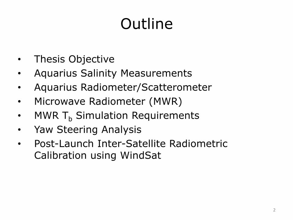
Outline

• Thesis Objective

• Aquarius Salinity Measurements

• Aquarius Radiometer/Scatterometer

• Microwave Radiometer (MWR)

• MWR Tb Simulation Requirements

• Yaw Steering Analysis

• Post-Launch Inter-Satellite Radiometric Calibration using WindSat

2

Thesis Objective

• Simulate realistic ocean brightness temperatures (Tb) for the 3-channel Microwave Radiometer (MWR) on Aquarius/SAC-D– To be used by CONAE for pre-launch

geophysical retrieval algorithms development

• Evaluate the proposed MWR measurement geometry and verify the requirements for spatial/temporal sampling

• Perform a preliminary study for the post-launch inter-satellite radiometric calibration using the WindSat radiometer as a reference

3

4

• Antenna

– Radiometer & Scatterometer share feeds and 2.5 m reflector

– Three footprints in pushbroom configuration

• Radiometer

– 1.413 GHz V, H-pol & 3rd Stokes

• Scatterometer

– 1.26 GHz H-pol

– Provides a critical correction for surface roughness

• Beams

– Inner – 76 x 94 Km

– Middle – 84 x 120 Km

– Outer – 96 x 156 Km

Aquarius Radiometer/Scatterometeron SAC-D

5

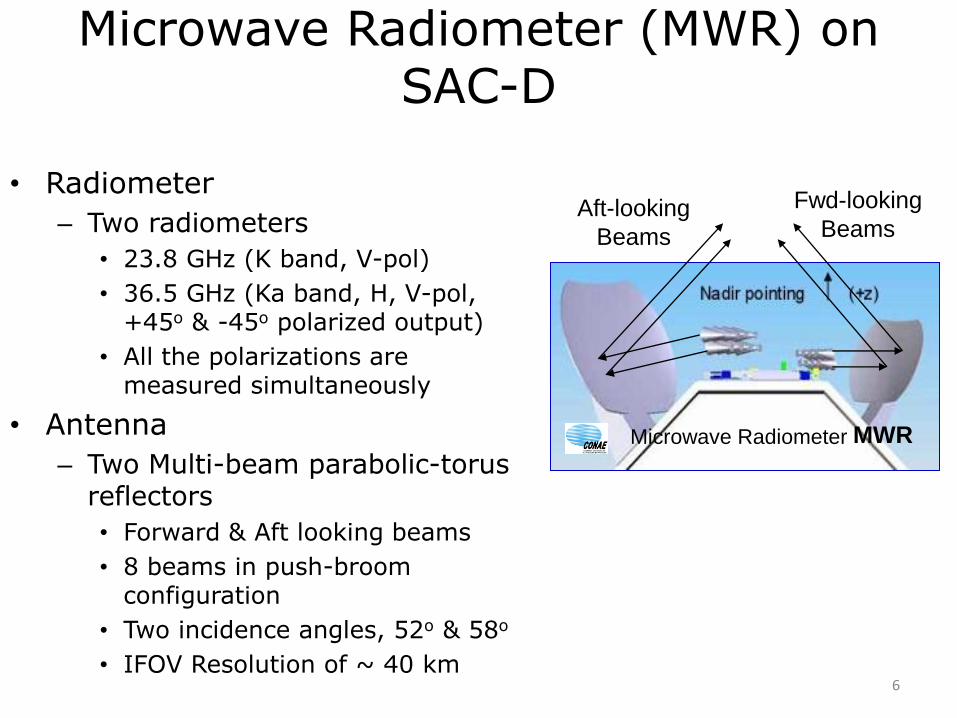
Microwave Radiometer (MWR) on SAC-D

• Radiometer

– Two radiometers

• 23.8 GHz (K band, V-pol)

• 36.5 GHz (Ka band, H, V-pol, +45o & -45o polarized output)

• All the polarizations are measured simultaneously

• Antenna

– Two Multi-beam parabolic-torus reflectors

• Forward & Aft looking beams

• 8 beams in push-broom configuration

• Two incidence angles, 52o & 58o

• IFOV Resolution of ~ 40 km

MWRMicrowave Radiometer

Aft-looking

Beams

Fwd-looking

Beams

6

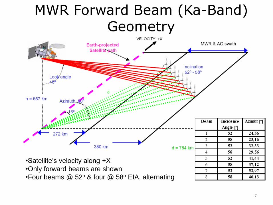
MWR Forward Beam (Ka-Band) Geometry

7

•Satellite’s velocity along +X

•Only forward beams are shown

•Four beams @ 52o & four @ 58o EIA, alternating

MWR Fwd & Aft Beam Geometry

Conical Arc

Conical Arc

8

58o

EIA

52o

EIA90o

MWR beams are sequentially sampled in time

In 1.92 sec, the beams move along-track by 13.1 Km

1.92 sec

9

•The sampling time made the simulation very challenging

since the beams are sampled sequentially at 0.24 sec

intervals in which the spacecraft (and hence the footprint)

moves as well

MWR Tb Simulation Requirements

10

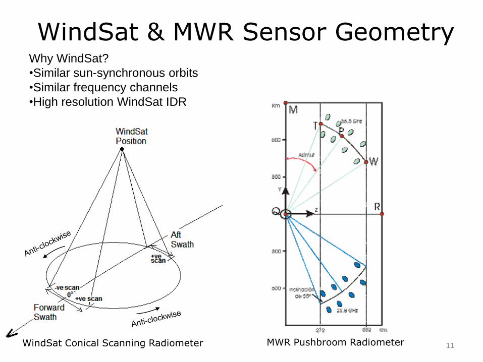
WindSat & MWR Sensor Geometry

WindSat Conical Scanning Radiometer MWR Pushbroom Radiometer 11

Why WindSat?

•Similar sun-synchronous orbits

•Similar frequency channels

•High resolution WindSat IDR

Conical Scanning Sensor Geometry

12

Conical Scanning Sensor Geometry cont.1

Antenna Beam IFOV

13

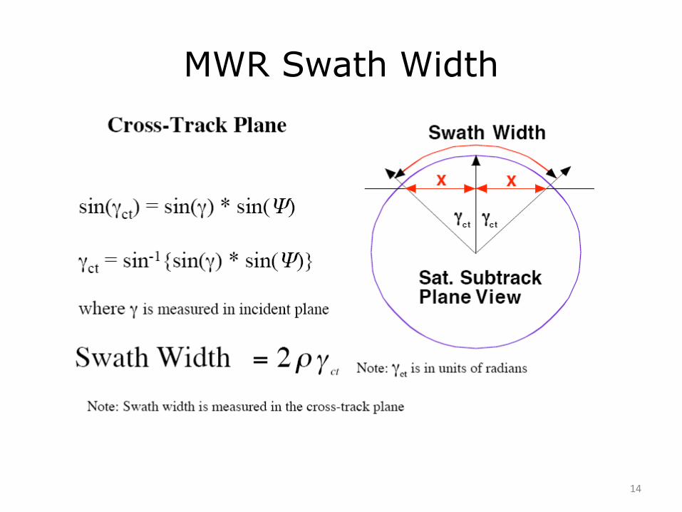
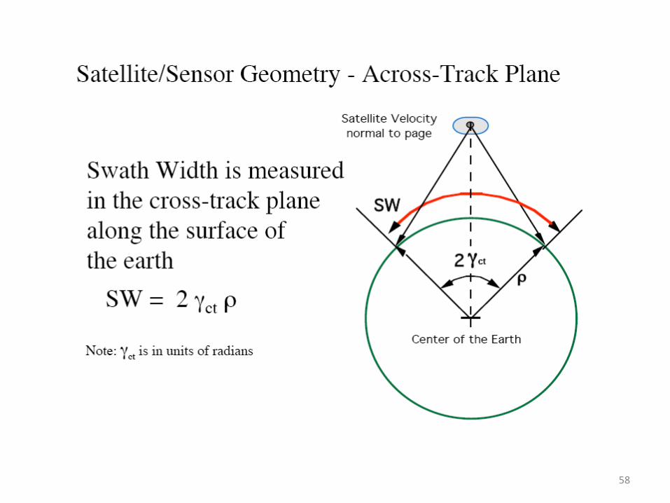
MWR Swath Width

14

Azimuthal Translation of MWR to Equivalent WindSat

15

Center of Earth

γ ct = 2.66o

γ ct = 5.58o

WindSat

MWR

ΔΨ WindSat

ΔΨ MWR

Satellite sub-track plane view

•Altitude WindSat = 840 Km

•Altitude MWR = 657 Km

•ΔΨ WindSat < ΔΨ MWR

MWR Swath Width

657 Km

840 Km

325.2 Km

Azimuthal Translation of MWR to Equivalent WindSat cont.

• MWR swath = 272 Km to 652 Km (to right of subtrack)

– corres ct = 2.66o to 5.58o

• Cross-track central angles ( ct) are the same for MWR and WindSat;

however central angles, () in the incident plane are different

– MWR 58 = 7.75°, 52 = 6.40°

– WindSat = 8.04o

• Using the equation,

solve for corresponding WindSat azimuth angles

Beam 1: Θ=52o

ψ=24.56o

Beam 8:Θ=58o

ψ=46.13o

sin ct sin sin

16

Beam-1

(Az, deg)

Beam-8

(Az, deg)

MWR 24.56 46.13

WindSat -19.37 -44.07

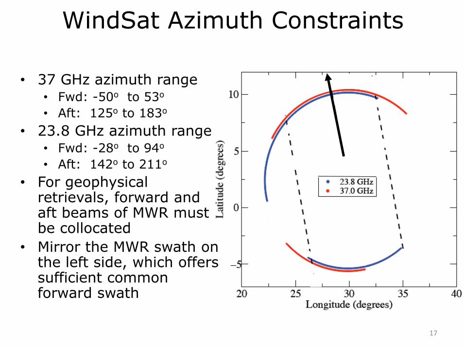
WindSat Azimuth Constraints

17

Longitude

La

titu

de

• 37 GHz azimuth range• Fwd: -50o to 53o

• Aft: 125o to 183o

• 23.8 GHz azimuth range• Fwd: -28o to 94o

• Aft: 142o to 211o

• For geophysical retrievals, forward and aft beams of MWR must be collocated

• Mirror the MWR swath on the left side, which offers sufficient common forward swath

WindSat Envir Data Record (EDR) Azimuth Constraints

• The EDR imposes a limit on the usable azimuth angles

• EDR azimuth range

-27.44o to 38.09o

• Left sided MWR mirrored swath will lose ~6o in azimuth; therefore swath is shifted to start from 38.09o

• Additional MWR beams generated using the entire azimuth range of EDR

18

-27.44o

38.09o

19.37o

44.06o

•Translated WindSat•EDR Azimuth Range

Flig

ht D

irection

WindSat EDR Azimuth Constraints• A total of 19 MWR beams

have been simulated

• 11 on the left & 8 on the right side of flight direction

• Left most MWR beam corresto swath width of 550.6 Km & right most corres to 411.1 Km

• The beam center to center swath spacing corres exactly to MWR spacing = 46.4 Km (325.2/ 7)

• Accurate spatial & sampling resolution of MWR

• Accurate orientation by change in azimuth

19

-27.44o38.09o EDR Azimuth Range

46.4 Km550.6 Km 411.1 Km

Flig

ht D

irection

•Beam Azimuth Angle:

γ ct = Swath width / ρ

Ψ beam= sin-1 (sin(γct)/sin(γ WindSat))

•The 8 beams on either side of flight direction are symmetrical by azimuth

58o EIA

52o EIA

53.8 54 54.2 54.4 54.6 54.8 55 55.2 55.4

5

5.1

5.2

5.3

5.4

5.5

5.6

5.7

5.8

5.9

6

Longitude

Latitu

de

23.8 GHz WindSat Intermediary Data Record

• High resolution spatial sampling along a conical scan

• Resolution 23 GHz - 12 x 20 Km

• Δψ 23.8 = 0.313o/pixel

20

54 54.2 54.4 54.6 54.8 55

5.2

5.3

5.4

5.5

5.6

5.7

5.8

5.9

Longitude

Latitu

de

37 GHz WindSat Intermediary Data Record

• High resolution spatial sampling along a conical scan

• Resolution 37 GHz - 8 x 13 Km

• Δψ 23.8 = 0.21o/pixel21

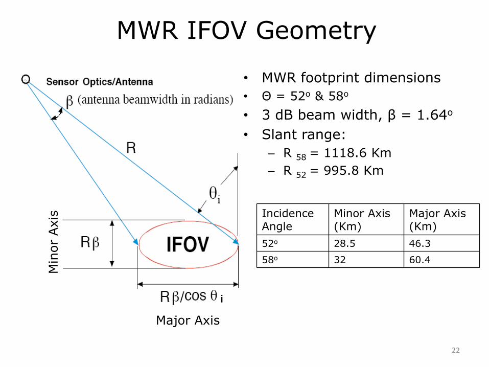
Incidence Angle

Minor Axis (Km)

Major Axis(Km)

52o 28.5 46.3

58o 32 60.4

MWR IFOV Geometry

• MWR footprint dimensions

• Θ = 52o & 58o

• 3 dB beam width, β = 1.64o

• Slant range:

– R 58 = 1118.6 Km

– R 52 = 995.8 Km

Min

or

Axis

Major Axis

22

56.6 56.7 56.8 56.9 57 57.1 57.2 57.3 57.4

-4

-3.9

-3.8

-3.7

-3.6

-3.5

-3.4

LONGITUDE

LA

TIT

UD

E

56.6 56.7 56.8 56.9 57 57.1 57.2 57.3 57.4

-4

-3.9

-3.8

-3.7

-3.6

-3.5

LONGITUDE

LA

TIT

UD

E

52o

52o

58o

58o

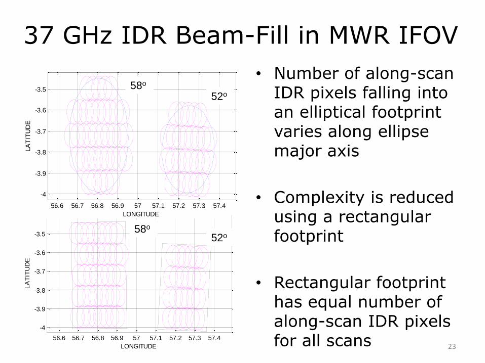
37 GHz IDR Beam-Fill in MWR IFOV

• Number of along-scan IDR pixels falling into an elliptical footprint varies along ellipse major axis

• Complexity is reduced using a rectangular footprint

• Rectangular footprint has equal number of along-scan IDR pixels for all scans 23

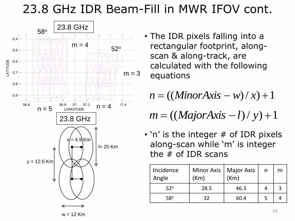
23.8 GHz IDR Beam-Fill in MWR IFOV cont.

• The IDR pixels falling into a rectangular footprint, along-scan & along-track, are calculated with the following equations

• ‘n’ is the integer # of IDR pixels along-scan while ‘m’ is integer the # of IDR scans

56.6 56.7 56.8 56.9 57 57.1 57.2 57.3 57.4

-3.9

-3.8

-3.7

-3.6

-3.5

-3.4

LONGITUDE

LA

TIT

UD

E

23.8 GHz

1)/)(( xwMinorAxisn

1)/)(( ylMajorAxism

52o

58o

m = 3

n = 4n = 5

m = 4

l= 20 Km

w = 12 Km

x = 4.9 Km

y = 12.6 Km

23.8 GHz

Incidence Angle

Minor Axis (Km)

Major Axis(Km)

n m

52o 28.5 46.3 4 3

58o 32 60.4 5 4

24

56.4 56.6 56.8 57 57.2 57.4

-5.3

-5.2

-5.1

-5

-4.9

-4.8

LONGITUDE

LA

TIT

UD

E

37 GHz IDR Beam-Fill in MWR IFOV cont.

37 GHz

52o

58o

m = 5

m = 4

n = 8n = 7

l = 13 Km

w = 8 Km

x = 3.3 Km

y = 12.6 Km

37 GHz

• The IDR pixels falling into a rectangular footprint, along-scan & along-track, are calculated with the following equations

• ‘n’ is the integer # of IDR pixels along-scan while ‘m’ is the integer # of IDR scans

1)/)(( xwMinorAxisn

1)/)(( ylMajorAxism

Incidence Angle

Minor Axis (Km)

Major Axis(Km)

n m

52o 28.5 46.3 7 4

58o 32 60.4 8 5

25

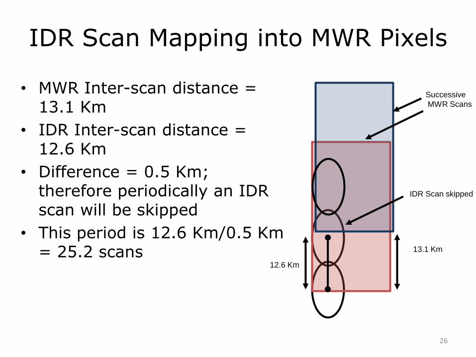
IDR Scan Mapping into MWR Pixels

• MWR Inter-scan distance = 13.1 Km

• IDR Inter-scan distance = 12.6 Km

• Difference = 0.5 Km; therefore periodically an IDR scan will be skipped

• This period is 12.6 Km/0.5 Km = 25.2 scans

12.6 Km

13.1 Km

IDR Scan skipped

26

Successive

MWR Scans

MWR IFOV Summary

Frequency Incidence Angle Width (Km) Length (Km) IDR Pixels n

(Across Track)

IDR Scans m

(Along Track)

23.8 GHz 58o 31.6 57.8 5 4

52o 26.7 45.2 4 3

37 GHz 58o 31.1 63.4 8 5

52o 27.8 50.8 7 4

56.6 56.7 56.8 56.9 57 57.1 57.2 57.3 57.4

-3.9

-3.8

-3.7

-3.6

-3.5

-3.4

LONGITUDE

LA

TIT

UD

E

23.8 GHz

52o

58o

m = 3

n = 4n = 5

m = 4

56.4 56.6 56.8 57 57.2 57.4

-5.3

-5.2

-5.1

-5

-4.9

-4.8

LONGITUDE

LA

TIT

UD

E

37 GHz

52o

58o

m = 5

m = 4

n = 8n = 7

27

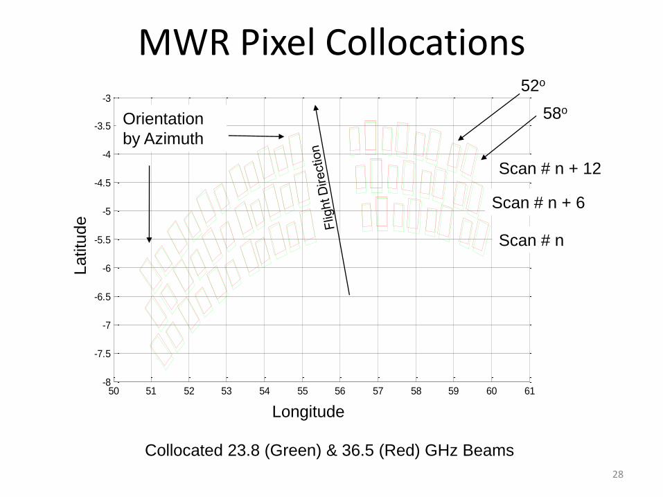
MWR Pixel Collocations

50 51 52 53 54 55 56 57 58 59 60 61-8

-7.5

-7

-6.5

-6

-5.5

-5

-4.5

-4

-3.5

-3

Longitude

Latitu

de

Longitude

Latitu

de

Collocated 23.8 (Green) & 36.5 (Red) GHz Beams

Orientation

by Azimuth

28

52o

58o

Scan # n

Scan # n + 6

Scan # n + 12

MWR 37 GHz Pixels

54 56 58 60 62 64

-25

-24.5

-24

-23.5

-23

-22.5

-22

-21.5

-21

-20.5

-20

Longitude

Latitu

de

MWR 36.5 GHz Swath at 58o (Red) & 52o (Green)

IDR Scan

Skip

IDR Scan

Skip

~ 25 scans

29

30

Start

WindSat IDR file

Filter out skipped IDR scans

Filtered WindSat IDR file

Filter WindSat IDR File

Beam 1…19 (θ, f, ψ)

Calculate Beam m, n (θ, f)

Find the along-scan IDR pixels(n, ψ)

Find the along-track range of scans(m)

Average Tb of IDR pixels

Average Tb of MWR Beams

MWR IFOV Summary

Get IDR Scan

Last scan?

No

Yes

MWR Tb

File

Store 19 MWR Beams of the scan

Comparison of WindSat & MWR Tb at 37 GHz (V-pol) @ 53 deg

100 200 300 400 500 600 700

100

200

300

100 200 300 400 500 600 700

100

200

300

200

250

300

200

250

300

WindSat Tb

MWR Tb

31

• 0.50 resolution

• Tb average of 68

obits in Feb 2007

• Shows radiometric

accuracy of the Tb

simulation

• Mean ΔTb = 0 K

• σ ΔTb = ~2 K

Tb Normalization

• WindSat Tb normalizations are required for incidence angle & frequency adjustment

– WindSat operates at 23.8 - & 37-GHz @ 53°

– MWR operates at 23.8 - & 36.5-GHz @ 52°& 58o

• Radiative Transfer Model (RTM) was used to transform WindSat Tb measurements to equivalent MWR frequencies and incidence angles

32

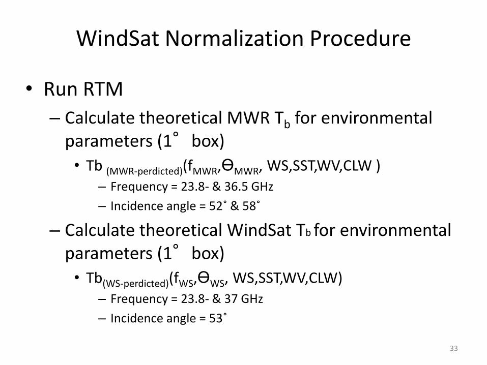
WindSat Normalization Procedure

• Run RTM

– Calculate theoretical MWR Tb for environmental parameters (1°box)

• Tb (MWR-perdicted)(fMWR,ƟMWR, WS,SST,WV,CLW )– Frequency = 23.8- & 36.5 GHz

– Incidence angle = 52˚ & 58˚

– Calculate theoretical WindSat Tb for environmental parameters (1°box)

• Tb(WS-perdicted)(fWS,ƟWS, WS,SST,WV,CLW)– Frequency = 23.8- & 37 GHz

– Incidence angle = 53˚

33

Expected Delta Tb (MWR to WindSat)

– Calculate the predicted (theoretical) Tb difference between MWR & WindSat

• delta = MWR predicted – WS predicted

Tb MWR = WindSat (measured) + delta

34

180 190 200 210 220 230 240 250 260

200

210

220

230

240

250

260

WindSat Tb (K)

MW

R T

b (

K)

Tb Normalization of 23.8 V Channel (58o)

45o Line

2nd order

regression

WindSat Tb(K)

MW

R T

b(K

)

35

WindSat Tb (K)

MW

R T

b (

K)

180 190 200 210 220 230 240 250 260

200

210

220

230

240

250

260

MW

R T

b(K

)

WindSat Tb(K)

MW

R T

b(K

)

•Ran RTM for 1 week to calculate WindSat & MWR theoretical Tb s

•Tb (theoretical) ( f, Ɵ, WS,SST,WV,CLW ), envr. parameters from GDAS

•Tb normalizations were done for all channels (23.8 V, 36.5 V & H) at 52o &

58o incidence angles

•The Tb Biases were found to be independent of the environmental

variables

Yaw Steering Results

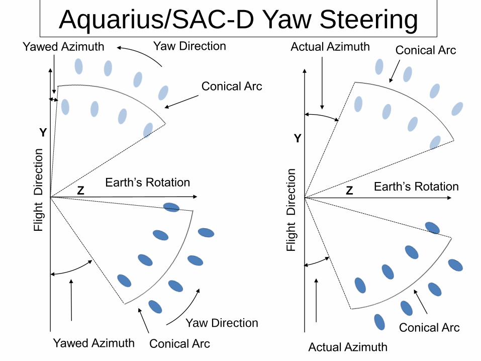
Yaw Direction

Flig

ht D

irection

Flig

ht D

irection

Y

Z

Y

Z

Aquarius/SAC-D Yaw Steering

Aquarius/SAC-D Yaw Steering

-100 -80 -60 -40 -20 0 20 40 60 80 1000

0.5

1

1.5

2

2.5

3

3.5

4

Latitude

Absolu

te Y

aw

(D

egre

es)

Absolute Yaw as a function of

Latitude (Provided by CONAE)Collocated MWR & Aquarius Swath

Earth’s Rotation

38

Latitude

Absolu

te Y

aw

(D

eg)

Max Yaw at Equator

Min Yaw at Poles

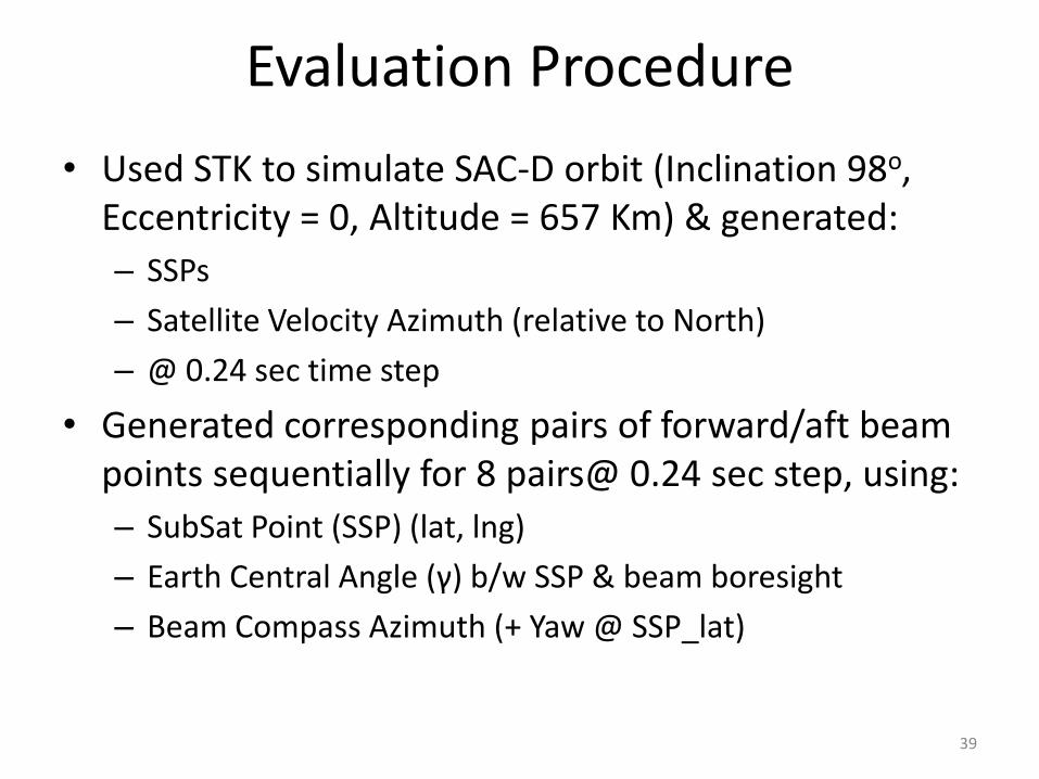
Evaluation Procedure

• Used STK to simulate SAC-D orbit (Inclination 98o,Eccentricity = 0, Altitude = 657 Km) & generated:

– SSPs

– Satellite Velocity Azimuth (relative to North)

– @ 0.24 sec time step

• Generated corresponding pairs of forward/aft beam points sequentially for 8 pairs@ 0.24 sec step, using:

– SubSat Point (SSP) (lat, lng)

– Earth Central Angle (γ) b/w SSP & beam boresight

– Beam Compass Azimuth (+ Yaw @ SSP_lat)

39

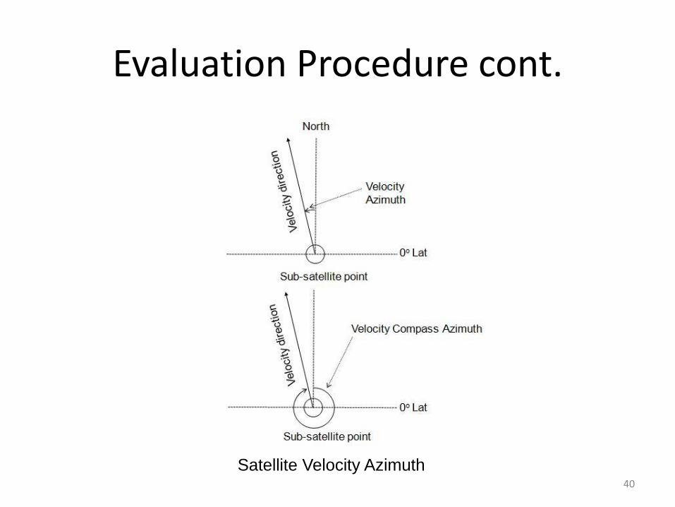
Evaluation Procedure cont.

Satellite Velocity Azimuth40

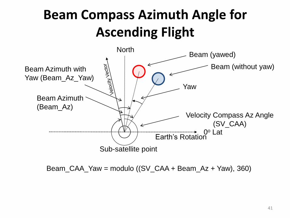
Beam Compass Azimuth Angle for Ascending Flight

Beam (yawed)

Beam (without yaw)

Yaw

Sub-satellite point

0o Lat

Velocity Compass Az Angle

(SV_CAA)

Beam Azimuth

(Beam_Az)

Beam Azimuth with

Yaw (Beam_Az_Yaw)

Beam_CAA_Yaw = modulo ((SV_CAA + Beam_Az + Yaw), 360)

Earth’s Rotation

North

41

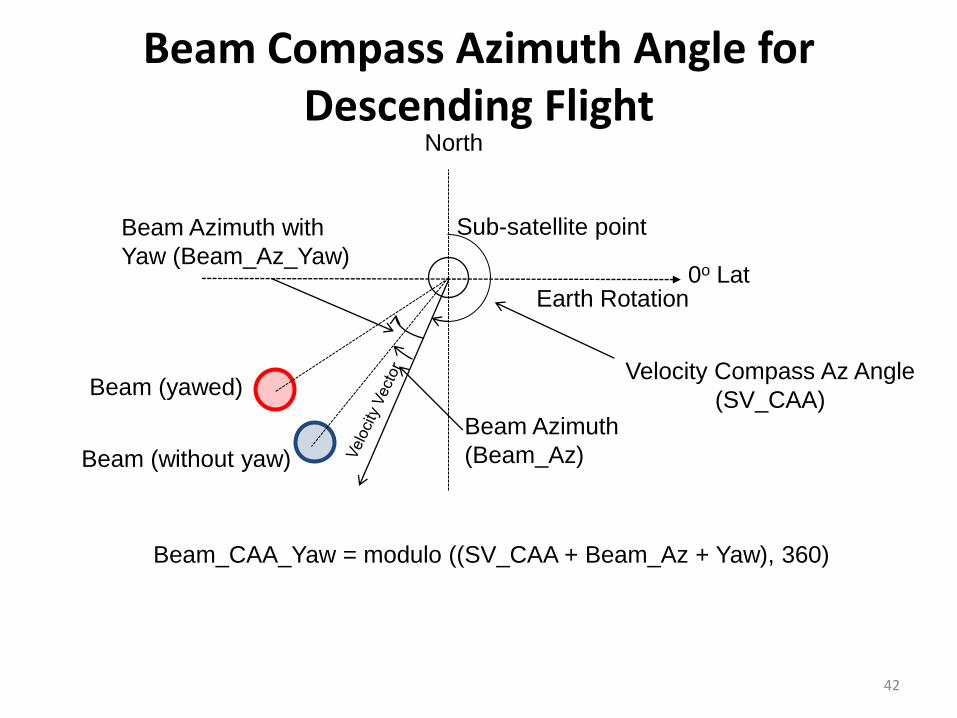
Beam Compass Azimuth Angle for Descending Flight

Beam (yawed)

Beam (without yaw)

Sub-satellite point

0o Lat

Velocity Compass Az Angle

(SV_CAA)Beam Azimuth

(Beam_Az)

Beam Azimuth with

Yaw (Beam_Az_Yaw)

Earth Rotation

North

42

Beam_CAA_Yaw = modulo ((SV_CAA + Beam_Az + Yaw), 360)

BEAM 1 ASC.

BEAM 1 DSC.

BEAM 8 ASC.

BEAM 8 DSC.

Beam-1 separation = 6 km Beam-8 separation = 2.2 km

Beam-8 separation = 6.1 km Beam-1 separation = 6 km

43

Forward/Aft Beam-1 Collocation Separation

Mean ~4 Km

Latitude

44

Collo

cation S

epara

tion (

Km

)•ASC

•DSC

Forward/Aft Beam-8 Collocation Separation

Dis

tance (

Km

)

Mean ~4.1 Km

Latitude

45

Collo

cation S

epara

tion (

Km

)•ASC

•DSC

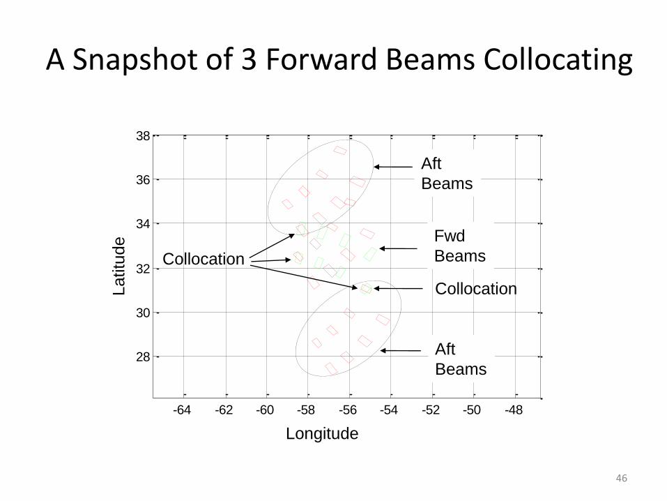
A Snapshot of 3 Forward Beams Collocating

-64 -62 -60 -58 -56 -54 -52 -50 -48

28

30

32

34

36

38

Longitude

Latitu

de Fwd

Beams

Aft

Beams

46

Aft

Beams

Collocation

Collocation

All Forward Beams Collocating withDifferent Aft Scans

47

-68 -66 -64 -62 -60 -58

55

56

57

58

59

Longitude

Latitu

de

Fwd Scan # 437

Aft Scan #:

Aft Scan #:536

558

529

552

519

543

504

530

Post-launch Inter-Satellite Radiometric Calibration using WindSat

48

WindSat shares similarities in orbit (ground track), radiometer frequencies and swath overlap with MWR

Parameter WindSat MWR

Altitude 840 Km 657 Km

Eccentricity 0.00134 0.0012

Inclination Angle 98.7o 98.01o

Ascending Node 6 p.m. 6 p.m.

Frequency23.8 (V & H) and 37.0 (V & H)

23.8 (V) and 36.5 (V & H) GHz

Swath Width ~950 Km ~380 Km

Earth Incidence Angle

53o 52o & 58o

49

50

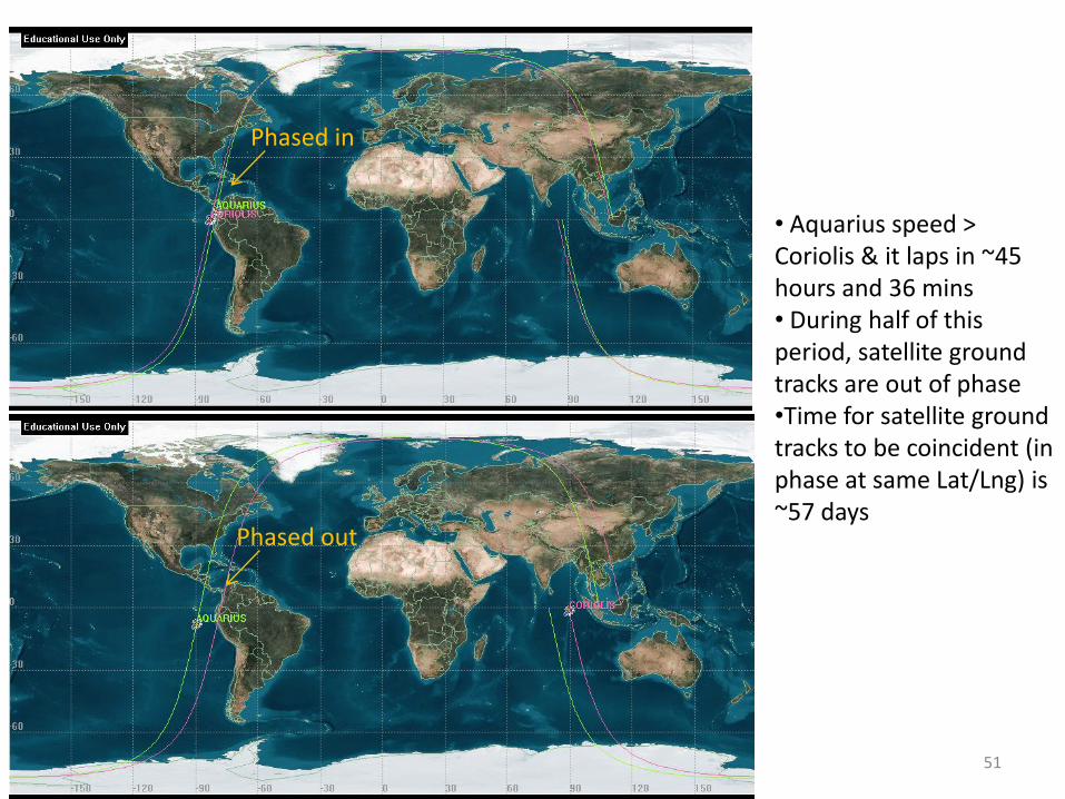
Phased in

Phased out

• Aquarius speed > Coriolis & it laps in ~45 hours and 36 mins • During half of this period, satellite ground tracks are out of phase•Time for satellite ground tracks to be coincident (in phase at same Lat/Lng) is ~57 days

51

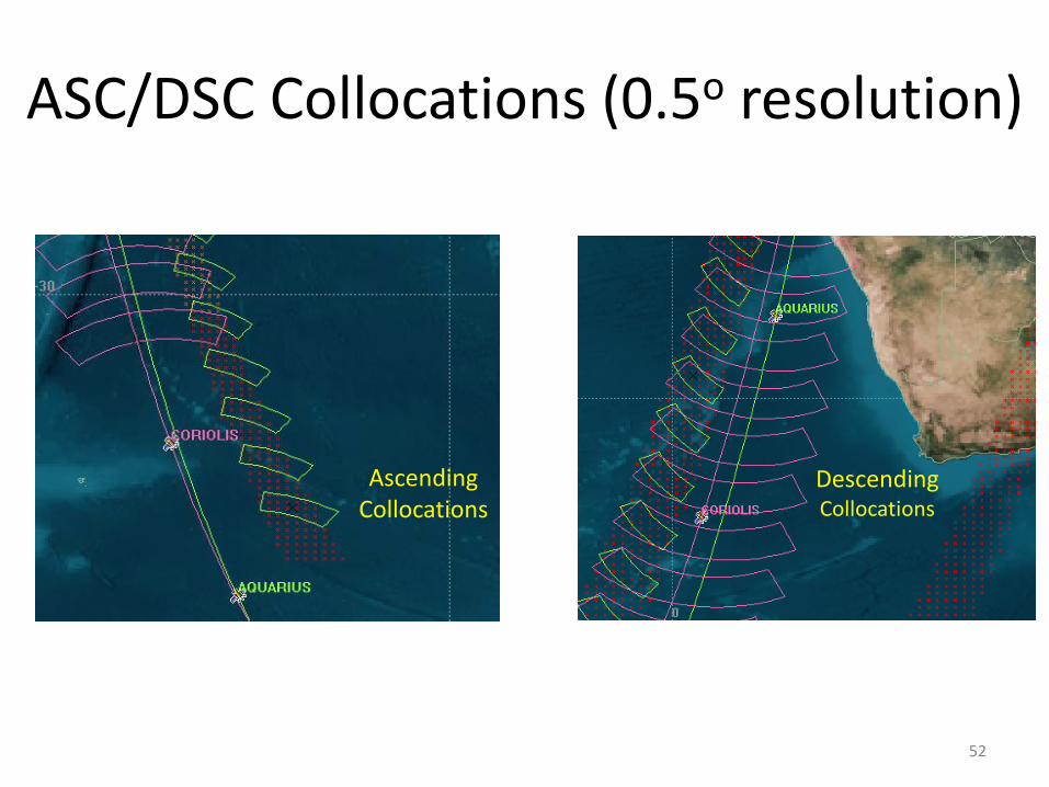
ASC/DSC Collocations (0.5o resolution)

52

Ascending Collocations

DescendingCollocations

• Approx 19,000 collocations in 45 hrs (± 50o Lat)• (0.5o x 0.5o) & ± 45 min window

• Approx 1 Million ocean collocations in 5 months

53

Conclusions

• The MWR Tb simulation is validated to have radiometric and temporal/spatial accuracy

• CONAE’s yaw steering technique to collocate the forward & aft MWR beams has also been verified with a mean collocation separation ~ 4 Km

• The inter-satellite swath collocation between WindSat and MWR shows that ~5 months in orbit, there will be ~1 Million ocean collocations

54

Future Work

• A four month simulated Tb dataset for the 3-channel MWR will be delivered to CONAE for the pre-launch geophysical retrieval algorithms development

• The MWR retrievals will be validated through near simultaneous, collocated comparisons with WindSat’s Environmental Data Records (EDRs)

55

Backup Slides

57

58

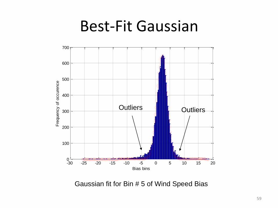
Best-Fit Gaussian

Gaussian fit for Bin # 5 of Wind Speed Bias

-30 -25 -20 -15 -10 -5 0 5 10 15 200

100

200

300

400

500

600

700

Bias bins

Fre

quency o

f occure

nce

Outliers Outliers

59