Simulation of Ant Routing Protocol for Ad-hoc networks in … · Simulation of Ant Routing Protocol ... 2.4.3 Ant-Colony Based Routing Algorithm ... this tree is used to build the

Faculty of Electrical Engineering, Mathematics and Computer Science

Network Architectures and Services Group

Simulation of Ant Routing Protocol

for Ad-hoc networks in NS-2

FJ Arbona BernatE-mail: <[email protected]>

November 2006

Supervisor: prof.dr.ir. P.F.A. Van Mieghem

Mentor: ir. S.S. Dhillon

Advisor: dr.ir. F.A. Kuipers

Copyright c© 2006 by FJ Arbona Bernat

All rights reserved. No part of the material protected by this copyright may be

reproduced or utilized in any form or by any means, electronic or mechanical, including

photocopying, recording or by any information storage and retrieval system, without the

permission from the author and Delft University of Technology.

ii

Abstract

Ant routing is a new scheme for routing inspired by the behavior of real ants. Real ants

are able to find the shortest path to a food source by following the trail of a chemical

substance called pheromone deposited by other ants. In ant routing, the ants (control

packets) collect information about the network conditions and are used to update and

maintain the routing tables.

The load balancing of routes used in ant routing has been proved successful in fixed

networks. This, together with the increasing popularity of ad-hoc wireless networks, has

given us the idea to adapt ant routing for such mobile networks and determine whether

it is suitable or not. A version of this ant routing protocol has been implemented to

work within the network simulator NS-2. Then, a performance comparison has been

done with two well-known ad-hoc routing protocols, i.e. AODV and DSR. Results show

that the overhead due to route maintenance is high, so the performance degrades and is

inferior to AODV and DSR. However, more simulations in another environment should

be done before rejecting this scheme for ad-hoc wireless networks.

Acknowledgements

I would like to thank my mentor, ir. S.S. Dhillon and my supervisor, Prof. P. Van

Mieghem, for guiding me throughout all my thesis project. They give me support and

helped me a lot to resolve the problems that have arised during my stay. Thanks for

their patience. I also want to mention my advisor, Dr. Fernando Kuipers, who guided

me during my whole exchange stay in TU Delft.

I am also grateful to my friends and fellow students, who give me their support in

and outside the laboratory. They are so many and from so different countries that I

cannot mention all of them. However, they know that I will always appreciate their

friendship and help.

Finally, but with no less enthusiasm, I want to dedicate this thesis to my family.

Specially to my mum and my sister, Cris, who, during our endless weekend phone

sessions, encouraged me to do my best to finish this thesis. And to my little nieces,

Esperanca and Victoria, who I look forward to see again soon.

But I cannot continue without mentioning my gratitude to all the anonymous people

who, one way or another, have inspired me for a better living. Not only in the academic

aspect of my life, but also in the personal and social one. Thanks!

iv

Contents

1 Introduction 1

1.1 Routing . . . . . . . . . . . . . . . . . . . . . . . . . . . . . . . . . . . . 1

1.2 Mesh networking . . . . . . . . . . . . . . . . . . . . . . . . . . . . . . . 2

1.3 Mobile Ad-hoc Networks . . . . . . . . . . . . . . . . . . . . . . . . . . . 3

1.4 Swarm Intelligence . . . . . . . . . . . . . . . . . . . . . . . . . . . . . . 4

1.5 Organization of the thesis . . . . . . . . . . . . . . . . . . . . . . . . . . 5

2 Related work 6

2.1 Destination-Sequenced Distance Vector (DSDV) . . . . . . . . . . . . . . 6

2.2 Dynamic Source Routing (DSR) . . . . . . . . . . . . . . . . . . . . . . . 7

2.3 Ad hoc On-Demand Distance Vector (AODV) . . . . . . . . . . . . . . . 8

2.4 Ant-based routing protocols . . . . . . . . . . . . . . . . . . . . . . . . . 8

2.4.1 Probabilistic Emergent Routing Algorithm (PERA) . . . . . . . . 9

2.4.2 Ant Agents for Hybrid Multipath Routing (AntHocNet) . . . . . 9

2.4.3 Ant-Colony Based Routing Algorithm (ARA) . . . . . . . . . . . 10

3 Implementation of Ant routing protocol 11

3.1 Network Model . . . . . . . . . . . . . . . . . . . . . . . . . . . . . . . . 12

3.1.1 Packet Classes and Structure . . . . . . . . . . . . . . . . . . . . 12

v

3.1.2 Node Structure . . . . . . . . . . . . . . . . . . . . . . . . . . . . 13

3.2 Algorithm Description . . . . . . . . . . . . . . . . . . . . . . . . . . . . 16

3.3 Neighbor Discovery Protocol (NDP) . . . . . . . . . . . . . . . . . . . . . 20

4 Simulations 21

4.1 Simulation environment . . . . . . . . . . . . . . . . . . . . . . . . . . . 22

4.1.1 Experiment Setup . . . . . . . . . . . . . . . . . . . . . . . . . . . 22

4.1.2 Running experiment . . . . . . . . . . . . . . . . . . . . . . . . . 25

4.1.3 Postprocessing results . . . . . . . . . . . . . . . . . . . . . . . . 27

4.1.4 Displaying results . . . . . . . . . . . . . . . . . . . . . . . . . . . 29

4.2 Experiments . . . . . . . . . . . . . . . . . . . . . . . . . . . . . . . . . . 30

4.2.1 AODV and DSR comparison . . . . . . . . . . . . . . . . . . . . . 30

4.2.2 Static scenario . . . . . . . . . . . . . . . . . . . . . . . . . . . . . 30

4.2.3 Mobile scenario . . . . . . . . . . . . . . . . . . . . . . . . . . . . 37

4.2.4 Large scenario . . . . . . . . . . . . . . . . . . . . . . . . . . . . . 39

5 Conclusions and Future Work 43

5.1 Conclusions . . . . . . . . . . . . . . . . . . . . . . . . . . . . . . . . . . 43

5.2 Recommendations for Future Work . . . . . . . . . . . . . . . . . . . . . 44

A Resum 45

A.1 Introduccio . . . . . . . . . . . . . . . . . . . . . . . . . . . . . . . . . . 46

A.2 Descripcio i implementacio de l’algoritme . . . . . . . . . . . . . . . . . . 47

A.3 Simulacions i resultats . . . . . . . . . . . . . . . . . . . . . . . . . . . . 48

vi

List of Tables

1.1 Reactive and proactive routing protocols . . . . . . . . . . . . . . . . . . 4

4.1 Basic settings of NS-2 simulations. . . . . . . . . . . . . . . . . . . . . . 26

4.2 Constants used in the DSR simulations . . . . . . . . . . . . . . . . . . . 26

4.3 Constants used in the AODV simulations . . . . . . . . . . . . . . . . . . 26

4.4 Example of user defined options of NS-2 simulations. . . . . . . . . . . . 27

4.5 Default scenario conditions. . . . . . . . . . . . . . . . . . . . . . . . . . 30

4.6 List of data connections . . . . . . . . . . . . . . . . . . . . . . . . . . . 33

4.7 List of neighbors in static scenario . . . . . . . . . . . . . . . . . . . . . . 33

vii

List of Figures

3.1 Node structure in NS-2 . . . . . . . . . . . . . . . . . . . . . . . . . . . . 14

3.2 Data structures . . . . . . . . . . . . . . . . . . . . . . . . . . . . . . . . 15

3.3 Squash function s(x) . . . . . . . . . . . . . . . . . . . . . . . . . . . . . 19

4.1 AODV-DSR comparison . . . . . . . . . . . . . . . . . . . . . . . . . . . 31

4.2 Node distribution in static scenario . . . . . . . . . . . . . . . . . . . . . 32

4.3 Average delay and PDR for a static scenario with 10 nodes. . . . . . . . 32

4.4 Optimal FA generation rate . . . . . . . . . . . . . . . . . . . . . . . . . 35

4.5 Optimal allowed HELLO loss . . . . . . . . . . . . . . . . . . . . . . . . 36

4.6 FA sent only during training period . . . . . . . . . . . . . . . . . . . . . 36

4.7 Tolerance to packet loss . . . . . . . . . . . . . . . . . . . . . . . . . . . 37

4.8 FA generation rate comparison . . . . . . . . . . . . . . . . . . . . . . . . 38

4.9 Pause-move periods . . . . . . . . . . . . . . . . . . . . . . . . . . . . . . 39

4.10 Sending FA only from known sources . . . . . . . . . . . . . . . . . . . . 40

4.11 Simulations on a larger scenario . . . . . . . . . . . . . . . . . . . . . . . 41

viii

Chapter 1

Introduction

Ad-hoc wireless networks are increasing in popularity, due to the spread of laptops,

sensor devices, PDAs and other mobile electronic devices. These devices will eventually

need to communicate with each other. In some cases, without an adequate infrastructure

to rely on. That’s why we need routing protocols that can work without any central

gateway to connect with.

At the same time, swarm intelligence has been used to solve optimization problems

applied to data networks. Routing is one such optimization problem where swarm intel-

ligence has been applied. Several routing protocols take advantage of that, i.e. AntNet

[7], ARA [15], AntHocNet [14] and PERA [3].

In this thesis we provide a fair comparison between an ant based routing protocol

(W AntNet) with other ad-hoc routing protocols, such as AODV [35] and DSR [5].

W AntNet is an adaptation of the AntNet algorithm proposed by Di Caro and Dorigo

in [7].

1.1 Routing

The term routing refers to the process of selecting paths in a computer network along

which to send data. This process can be splitted in a routing protocol, used to exchange

information about topology and link weights, and a routing algorithm, that actually

computes paths between nodes [28].

1

2 CHAPTER 1. INTRODUCTION

There are mainly two approaches for routing algorithms, distance-vector algorithms

and link-state algorithms. The former, like Bellman Ford’s algorithm, assigns a number,

called cost, to each of the links between every node in the network. Nodes will send

information from a source node S to a destination D via the path with the lowest total

cost. An example of the latter is Dijkstra’s algorithm, which uses a data structure that

contains all nodes. It starts with a tree containing only itself. Then, one at a time, from

the set of nodes which it has not yet added to the tree, it adds the node which has the

lowest cost to reach an adjacent node which already appears in the tree. This continues

until every node appears in the tree. Then, this tree is used to build the routing table.

An example of the classical approach to routing is the Open Shortest Path First

(OSPF) protocol. In OSPF, the routers exchange link-state information by flooding the

network. The link state updates are generated only when the link status changes. Once

a node has obtained topology information of the entire network, Dijkstra’s algorithm is

generally used to compute the shortest path.

The two main performance metrics that are affected by the routing algorithm are

throughput (quantity of service) and average packet delay (quality of service) [4]. Routing

is a complex task. Coordination is needed between nodes, link and nodes can fail, and

congestion can arise in some areas. Thus, the routing algorithm needs to modify its

routes, redirecting traffic and updating databases.

1.2 Mesh networking

Mesh networking is a popular term for multi-hop wireless networks used to solve the

problem of how to provide broadband connections to homes without running cables

directly to each subscriber [10]. At the moment, the main option is to reuse the tele-

phone or cable-TV networks. Mesh networking is an approach being proposed by both

commercial and open-source/community movements.

In the commercial model, a neighborhood access point (NAP) is installed, which is

a radio base station with a high-speed internet connection. Subscribers to the service

install their own wireless node to gain access to the NAP. Once this node is installed, it

can also act as a relay to extend the effective coverage of the NAP.

1.3. MOBILE AD-HOC NETWORKS 3

1.3 Mobile Ad-hoc Networks

Mobile ad-hoc networks (MANETs) are self-organized networks. Communication in an

ad-hoc network does not require existence of a central base station or a fixed network

infrastructure. Each node of an ad-hoc network is both a host and a router. That is,

the destination of some information packets while at the same time it can function as

relay station for other packets to their final destination.

This multi-hop support in ad-hoc networks, which makes communication between

nodes outside direct radio range of each other possible, is probably the most distinct

difference between mobile ad-hoc networks and wireless LANs. The MANETs main

characteristics [9] are:

Dynamic topologies Nodes are free to move randomly and organise themselves arbi-

trarily. Thus, the network topology, typically multihop, may change rapidly and

unpredictably. That leads towards the need of an effective routing, a challenging

problem to solve.

Bandwidth-constrained, variable capacity links Wireless links, which can be ei-

ther bidirectional or unidirectional, will continue to have significantly lower capac-

ity than wired ones. In addition, the actual throughput of wireless communications–

after accounting for the effects of multiple access, fading, noise, and interference

conditions, etc.–is often much less than a radio’s maximum transmission rate.

One effect of the relatively low to moderate link capacities is that congestion is

typically the norm rather than the exception, so demand from users will likely

approach or exceed network capacity frequently. As the mobile network is often

simply an extension of the fixed network infrastructure, mobile ad hoc users will

demand similar services. These demands will continue to increase as multimedia

computing and collaborative networking applications rise.

Energy-constrained operation Some or all of the nodes in a MANET may rely on

batteries or other exhaustible means for their energy. For these nodes, the most

important system design criteria for optimization may be energy conservation. As

a result, routing algorithms should be as simple as possible to avoid intensive

computations. For example, overhearing transmissions requires a large amount of

energy to receive and decode entire packets.

4 CHAPTER 1. INTRODUCTION

Limited physical security Mobile wireless networks are generally more prone to phys-

ical security threats than wired nets. The increased possibility of eavesdropping,

spoofing, and denial-of-service attacks should be carefully considered. Existing link

security techniques are often applied within wireless networks to reduce security

threats. As a benefit, the decentralized nature of network control in MANETs pro-

vides additional robustness against the single points of failure of more centralized

approaches.

Scalability Networks may be large, normally more than 10 nodes and reaching 1000

nodes in a sensor network. Thus, routing protocols should be able to scale [32] to

this amount.

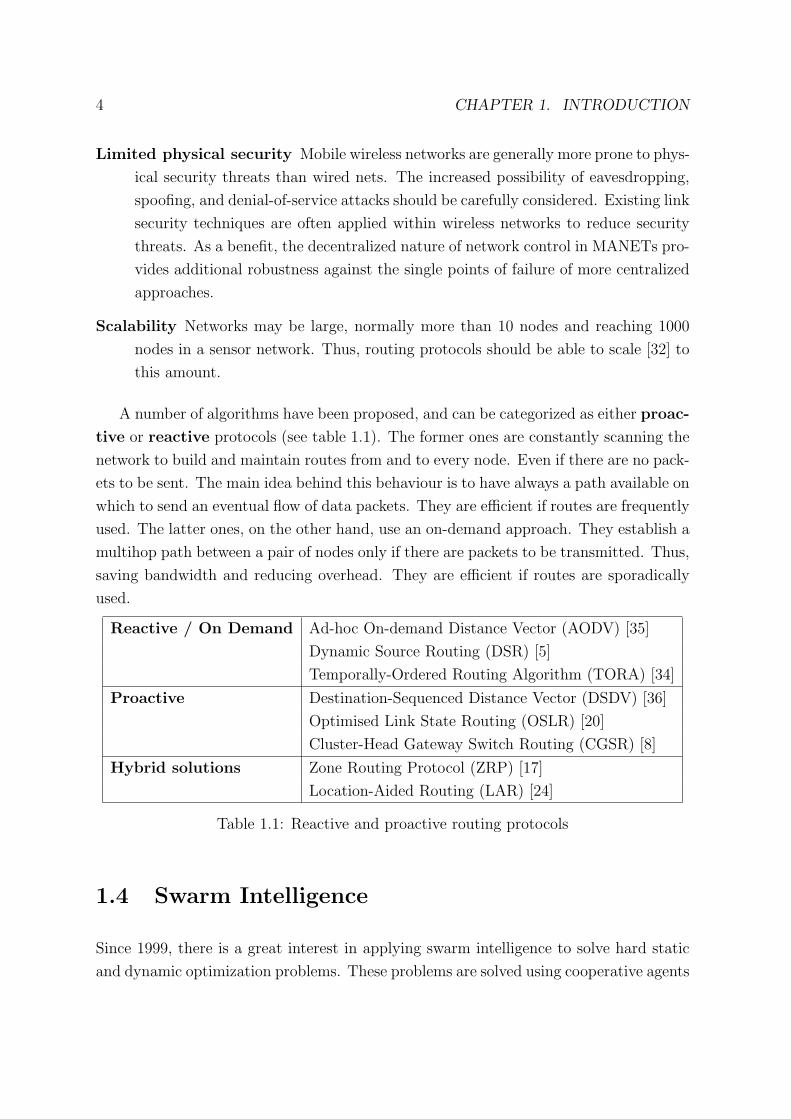
A number of algorithms have been proposed, and can be categorized as either proac-

tive or reactive protocols (see table 1.1). The former ones are constantly scanning the

network to build and maintain routes from and to every node. Even if there are no pack-

ets to be sent. The main idea behind this behaviour is to have always a path available on

which to send an eventual flow of data packets. They are efficient if routes are frequently

used. The latter ones, on the other hand, use an on-demand approach. They establish a

multihop path between a pair of nodes only if there are packets to be transmitted. Thus,

saving bandwidth and reducing overhead. They are efficient if routes are sporadically

used.

Reactive / On Demand Ad-hoc On-demand Distance Vector (AODV) [35]

Dynamic Source Routing (DSR) [5]

Temporally-Ordered Routing Algorithm (TORA) [34]

Proactive Destination-Sequenced Distance Vector (DSDV) [36]

Optimised Link State Routing (OSLR) [20]

Cluster-Head Gateway Switch Routing (CGSR) [8]

Hybrid solutions Zone Routing Protocol (ZRP) [17]

Location-Aided Routing (LAR) [24]

Table 1.1: Reactive and proactive routing protocols

1.4 Swarm Intelligence

Since 1999, there is a great interest in applying swarm intelligence to solve hard static

and dynamic optimization problems. These problems are solved using cooperative agents

1.5. ORGANIZATION OF THE THESIS 5

that communicate with each other modifying their environment, like ant colonies or

others insects do. That is why these agents are commonly called ants.

Key characteristics of these models are:

• Large numbers of simple agents.

• Agents may communicate with each other directly.

• Agents may communicate indirectly by affecting their environment, a process

known as stigmergy.

• Intelligence contained in the networks and communications between agents.

• Local behavior of agents causes some emergent global behavior 1.

Ant routing is the result of using swarm-intelligence in systems for routing within

communications networks. AntNet [7], a particular ant routing algorithm was tested

in routing for fixed networks with a better performance than OSPF, asynchronous dis-

tributed Bellman-Ford with dynamic metrics, shortest path with dynamic cost metric,

Q-R algorithm and predictive Q-R algorithm.

1.5 Organization of the thesis

First, in Chapter 2, we will introduce some other routing solutions for MANETs. Then,

in chapter 3, we will discuss the implementation of our ant routing protocol in NS-2

[19]. Afterwards, in chapter 4, we will show our performance comparison results that,

for practical reasons, have been obtained by simulation. Finally, in chapter 5, we will

present our conclusions and recommendations for future work.

In addition, a summary in Catalan is provided in appendix A, at the end of this

thesis document.

1For example, crickets tend to sync their mating calls, calling all at once at the same speed or birdsflying around can create large groups of birds that seem to behave as one.

Chapter 2

Related work

2.1 Destination-Sequenced Distance Vector (DSDV)

DSDV is a hop-by-hop distance vector routing protocol. It is proactive and each node has

to periodically broadcast routing updates. The key advantage of DSDV over traditional

distance vector protocols is that it guarantees loop-freedom by using the concept of

sequence numbers.

Each DSDV node maintains a routing table listing the “next hop” for each reachable

destination. DSDV tags each route with a sequence number and considers a route R

more favourable than R′ if R has a greater sequence number, or if the two routes have

equal sequence number but R has a lower metric. Each node in the network advertises

an increasing even sequence number for itself. When a node nB decides its route to

a destination nd is broken, it advertises the route to nd with an infinite metric and a

sequence number one greater than its sequence number for the route that has broken

(making an odd sequence number). This causes any node nA routing packets through

nB to incorporate the infinite-metric route into its routing table until node nA hears a

route to nd with a higher sequence number.

DSDV uses triggered route updates when the topology changes. The transmission of

updates is delayed to introduce a softening effect when the topology is changing quickly.

This gives an additional adaptation of DSDV to ad-hoc networks.

6

2.2. DYNAMIC SOURCE ROUTING (DSR) 7

2.2 Dynamic Source Routing (DSR)

DSR [5] is a reactive protocol that uses source routing rather than hop-by-hop routing,

with each packet to be routed carrying in its header the complete, ordered list of nodes

through which the packet must pass. The key advantage of source routing is that

intermediate nodes do not need to maintain up-to-date routing information in order

to route the packets they forward, since the packets themselves already contain all

the routing decisions. This fact, coupled with the on-demand nature of the protocol,

eliminates the need for the periodic route advertisement and neighbor detection packets

present in other protocols. However, routing overhead is bigger.

The DSR protocol consists of two mechanisms: Route Discovery and Route Maintenance.

Route Discovery is the mechanism by which a node ns wanting to send a packet to

a destination nd obtains a path. To perform a Route Discovery, the source node ns

broadcasts a Route Request packet that is flooded through the network in a controlled

manner and is answered by a Route Reply packet from either the destination node

or another node that knows a route to the destination. To reduce the cost of Route

Discovery, each node mantains and actively uses a cache of source routes it has learned

or overheard. That way, the frequency and propagation of Route Requests is limited.

Route Maintenance is the mechanism by which a packet’s sender ns detects if the

network topology has changed such that it can no longer use its route to the destination

nd because two nodes listed in the route have moved out of range of each other. When

Route Maintenance indicates a source route is broken, ns is notified with a Route Error

packet. The sender ns can attempt to use any other route to nd already in its cache or

can invoke Route Discovery again to find a new path.

A DSR node is able to learn routes by overhearing packets not addressed to it (the

promiscuous mode). However, this feature requires an active receiver in the nodes, which

may be rather power consuming and apparently does not improve performance [21].

The implementation used in our simulations is the same it comes by default with

NS-2 version 2.29.

8 CHAPTER 2. RELATED WORK

2.3 Ad hoc On-Demand Distance Vector (AODV)

AODV is essentially a combination of both DSR and DSDV. It borrows the basic on-

demand mechanism of Route Discovery and Route Maintenance from DSR, plus the

use of hop-by-hop routing, sequence numbers, and periodic beacons from DSDV.

When a node ns needs a route to some destination nd, it broadcasts a Route Request

message to its neighbors, including the last known sequence number for that destina-

tion. The Route Request is flooded until it reaches a node that knows a route to the

destination. Each node that forwards the Route Request creates a reverse route for

itself back to node ns.

When the Route Request reaches a node with a route to nd, that node generates a

Route Reply that contains the number of hops necessary to reach nd and the sequence

number for nd most recently seen by the node generating the Reply. Each node that

participates in forwarding this Reply back toward the originator of the Route Request

(node ns), creates a forward route to nd. The state created in each node along the path

from ns to nd is hop-by-hop state; that is, each node remembers only the next hop and

not the entire route, as would be done in source routing.

In order to maintain routes, AODV normally requires that each node periodically

transmit a HELLO message, with a default rate of once per second. Failure to receive

three consecutive HELLO messages from a neighbor is taken as an indication that the link

to the neighbor is down. Alternatively, the AODV specification briefly suggests that a

node may use physical layer or link layer methods to detect link breakages to nodes that

it considers neighbors [35].

When a link goes down, any upstream node that has recently forwarded packets to

a destination using that link is notified via an Unsolicited Route Reply containing an

infinite metric for that destination. Upon receipt of such a Route Reply, a node must

acquire a new route to the destination using Route Discovery as described above.

2.4 Ant-based routing protocols

Apart from AODV, DSDV and DSR, there are also some initiatives for ant-routing in

ad-hoc networks as PERA [3], AntHocNet [14] or ARA [15, 16].

2.4. ANT-BASED ROUTING PROTOCOLS 9

2.4.1 Probabilistic Emergent Routing Algorithm (PERA)

This algorithm exploits the inherent broadcast capability of wireless networks to reach

a better performance. The route discovery and maintenance is done by flooding the

network with ants. Both forward and backward ants are used to fill the routing tables

with probabilities. These probabilities reflect the likelihood that a neighbor will forward

a packet to the given destination. Also multiple paths between source and destination

are created.

First of all, neighbors are discovered using HELLO messages, but entries are only

inserted in the routing table after receiving a backward ant from the destination node.

Each neighbor receives an equiprobable value for destination. This value is increased as

a backward ant comes from that node, establishing a path towards destination.

As ants are flooded, the algorithm uses sequence numbers to avoid duplicate packets.

Only the greater sequence number from the same previous hop is taken into account.

Forward ants with a lower sequence number are dropped. This approach is similar to

AODV Route Request packets, but discovers a set of routes instead of one.

Data packets can be routed according to the highest probability in the routing table

for the next hop, or stochastically, that performs better in fixed networks with small

topologies.

2.4.2 Ant Agents for Hybrid Multipath Routing (AntHocNet)

AntHocNet is a multipath routing algorithm for mobile ad-hoc networks that combines

both proactive and reactive components. It is based on AntNet [7], designed for wired

networks, with some modifications to be used on ad-hoc networks. For example, it

does not maintain routes to all possible destinations at all times, but only for the open

data sessions. This is done in a Reactive Route Setup phase, where reactive forward

ants are sent by the source node to find multiple paths towards the destination node.

Backward ants are used to actually setup the route. While the data session is open,

paths are monitored, maintained and improved proactively using different agents, called

proactive forward ants. The algorithm reacts to link failures with either a local route

repair or by warning preceding nodes on the paths.

10 CHAPTER 2. RELATED WORK

2.4.3 Ant-Colony Based Routing Algorithm (ARA)

The protocol is based on swarm intelligence and especially on the ant colony based meta

heuristic. The routing algorithm consists of three phases.

In the first one, Route Discovery Phase, new paths are discovered. The creation of

new routes requires the use of a forward ant (FANT), which establishes the pheromone

track to the source node, and a backward ant (BANT), which establishes the track to the

destination node. FANTs are broadcasted by the sender to all its neighbors. Each FANT

has a unique sequence number to avoid duplicates. A node receiving a FANT for the

first time, creates a record (destination address, next hop, pheromone value) in

its routing table. The node interprets the source address of the FANT as destination

address, the address of the previous node as next hop, and computes the pheromone

value depending on the number of hops the FANT needed to reach the node. Then

the node relays the FANT to its neighbors. When the FANT reaches destination, it

is processed in a special way. The destination node extracts the information and then

destroys the FANT. A BANT is created and sent towards the source node. In that way,

the path is established and data packets can be sent.

In the second phase, called Route Maintenance, routes are improved during com-

munication. Data packets are used to maintain the path, so no overhead is introduced.

Pheromone values are changing. When a node vi relays a data packet toward destination

vD to a neighbor node vj, it increases the pheromone value of the entry (vD, vj, ψ) by

δψ. The same happens in the opposite direction. The evaporation process is simulated

by regular decreasing of the pheromone values.

The third one handles routing failures, due especially to node mobility, a common

issue in MANETs. ARA recognizes a route failure through a missing acknowledgement.

The links are deactivated by setting to 0 the pheromone value. Then the node searches

for an alternative link. If a second path exists, it is used. Otherwise, neighbors are

informed of the new situation.

ARA fulfills the requirements of distributed operation, loop-freeness, on demand

operation and sleep period operation (that is, nodes are able to sleep when their amount

of pheromone reaches a threshold). Moreover, routing entries and statistic information

are local to each node, several paths are maintained to reach a certain destination and,

in a node with sleep mode on, only packets destined to it are processed.

Chapter 3

Implementation of Ant routing

protocol

While other ad-hoc routing protocols like AODV, DSR or DSDV were already developed

in NS-2, no ant routing protocol was. Thus, the first step was to implement a routing

agent and integrate it in the NS-2 simulator.

After reading some papers related to ant protocols and algorithms [15, 14, 7] we have

decided to implement a modified version of AntNet [7]. The modifications are needed

because AntNet has been designed for fixed networks and we are going to use it in ad-hoc

networks, where the topology is highly dynamic. Thus, we added a neighbor discovery

protocol and some mechanisms to deal with mobility. The core algorithm has not been

altered, and we have applied the same parameters and recomendations as our paper of

reference.

Some people [10, 39] had already implemented a similar protocol in NS-2, but their

motivation was different. Nevertheless, we have used their code as inspiration, as well

as the code for AODV, already implemented in NS-2, to have some coherence with the

backbone of the simulator.

In [29], a simulator was developed specifically for ant routing. However, this sim-

ulator was not taking care of MAC layer nor implementing AODV or DSR, Thus, no

performance comparison was done.

The version used to develop our routing agent is ns-2.29, the most recent release when

we started coding. We have used the programming language C++ to code the main

11

12 CHAPTER 3. IMPLEMENTATION OF ANT ROUTING PROTOCOL

routines of the routing agent, and oTCL to modify the parameters during simulations.

The Network Simulator 2 (NS-2) [19] has been chosen because of its popularity among

academic researchers. Other available simulators are QualNet [37], OPNET [33] and

GloMoSim [11, 1].

To avoid confusions with previous implementations of ant routing protocol, we will

call our implementation W AntNet (Wireless AntNet) in the following.

3.1 Network Model

3.1.1 Packet Classes and Structure

The packets used in the network can be divided into three different classes:

Data packets represent the information that the end-users exchange with each other.

In ant-routing, data packets do not maintain any routing information but use the

information stored at routing tables for travelling from the source to the destination

node.

Forward and Backward ants are control packets used to update the routing tables

and distribute information about the traffic load in the network.

Neighbor Control packets are used to maintain a list of available nodes to which

forward packets. Actually, they are HELLO messages broadcasted periodically

from each node to all its neighbors.

The data packets are normal IP packets. Thus, we will not consider their internal

structure. We will rather center our attention to control packets, both routing agents

and neighbor control packets (NCP).

Neighbor Control packets are rather simple, as their only purpose is to serve as

HELLO messages to indicate the presence of a node in the network. They contain only

the source address and an identifier to distinguish them from the routing agents.

Routing agents, both forward and backward ants, contain, in addition to the IP

header, the following data fields:

3.1. NETWORK MODEL 13

Final destination address towards where the original forward ant was sent. It is

necessary to check if the ant has arrived or not, as the IP destination address will

change at every visited node.

Birthtime is the time when the ant has been generated.

Arrival time to the final destination. This value is used to calculate the trip time.

Memory stack with the addresses of the visited nodes and the departure time towards

the nexthop.

3.1.2 Node Structure

Every node in the network maintains a structure as stated in chapter 5 of [23] (see Fig.

3.1). In addition, there are an input buffer composed of a single queue and an output

buffer composed of a high priority queue and a low priority queue for each neighbor or

outgoing link. The high priority queue is served before the low priority queue.

When a node receives a packet from a neighbor, the packet is first stored in the

input buffer. The packet in the input buffer is served in a FIFO order. After the packet

has been served, the packet is sent to the output buffer. Within the output buffer, the

packet goes to a particular queue for a particular outgoing link based on the type of

the packet and the next node. Backward ant packets have a higher priority than the

data and forward ant packets and are thus stored in the high priority queue, while data

and forward ant packets are stored in the low priority queue. The maximum number of

packets stored in the input or output buffer is limited by the size of the buffer. So, if

the buffer is full, packets are dropped.

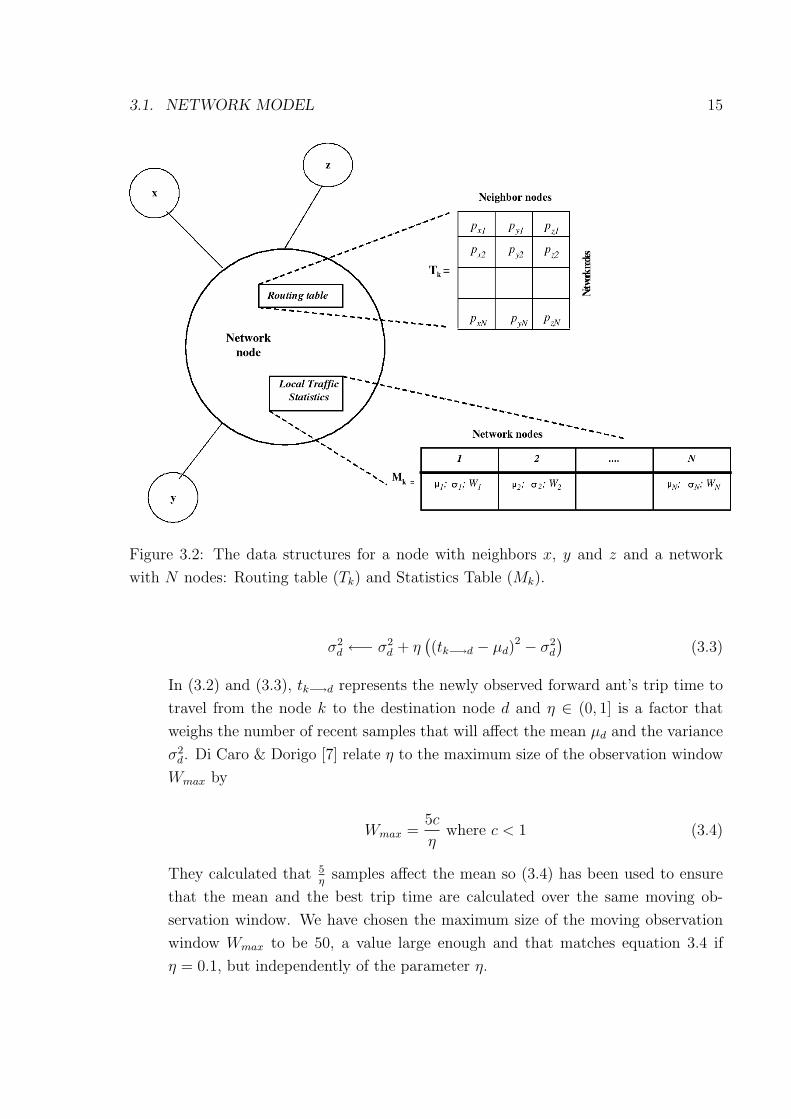
Furthermore, each node has two data structures (see Fig. 3.2) which the routing

agents can interact with in an indirect way:

• One of them is a routing table Tk containing triples of a destination address d, a

nexthop n used to reach that destination d and a probability Pnd. This probability

value Pnd stored in the routing table express the goodness of choosing the associated

nexthop n to reach the destination d. The probabilities have to verify:

∑n∈Nk

pnd = 1 (3.1)


Figure 3.1: Node structure in NS-2.

where d ∈ [1, N ] and Nk = {neighbors (k)}.

• The other one is a local traffic model Mk, containing the statistics about the

network topology and traffic distribution by means of the measured delay. The

model is adaptative and described by means and variances computed over the

trip times experienced by the agents. A windowing mechanism is used to limit

the number of samples used. For each destination d in the network, the table Mk

contains a moving observation windowWd, an estimated mean µd and an estimated

variance σ2d. The moving observation window Wd, of size Wmax, represents an array

containing the trip times of the lastWmax forward ants that travelled from the node

k to the destination d. The moving observation window Wd is used to compute

the best trip time tbestd experienced by a forward ant travelling from the node k to

the destination d among the last Wmax forward ants that travel from the node k to

the destination d. The mean µd and variance σ2d represent the mean and variance

of the trip times experienced by the forward ants to move from the node k to the

destination node d and are calculated using the exponential model:

µd ←− µd + η (tk−→d − µd) (3.2)

3.1. NETWORK MODEL 15

Figure 3.2: The data structures for a node with neighbors x, y and z and a network

with N nodes: Routing table (Tk) and Statistics Table (Mk).

σ2d ←− σ2

d + η((tk−→d − µd)

2 − σ2d

)(3.3)

In (3.2) and (3.3), tk−→d represents the newly observed forward ant’s trip time to

travel from the node k to the destination node d and η ∈ (0, 1] is a factor that

weighs the number of recent samples that will affect the mean µd and the variance

σ2d. Di Caro & Dorigo [7] relate η to the maximum size of the observation window

Wmax by

Wmax =5c

ηwhere c < 1 (3.4)

They calculated that 5η

samples affect the mean so (3.4) has been used to ensure

that the mean and the best trip time are calculated over the same moving ob-

servation window. We have chosen the maximum size of the moving observation

window Wmax to be 50, a value large enough and that matches equation 3.4 if

η = 0.1, but independently of the parameter η.


3.2 Algorithm Description

The W AntNet algorithm, which is basically the same as the AntNet [7] algorithm1, can

be described in detail as follows:

1. At regular intervals, from every network node s, a forward ant Fs−→d is launched

towards a randomly selected destination node d. Destinations are chosen to match

the current traffic patterns i.e., if fsd is a measure (in bits or in the number of

packets) of the data flow s −→ d, then the probability yd of creating at node s a

forward ant with node d as destination is:

yd =fsd∑N

d′=1 fsd′

(3.5)

2. While travelling towards their destination nodes, the forward ants store the address

of each visited node Nk and the departure time to the next hop in a memory stack.

Forward ants share the same queues as data packets, so they experience the same

traffic delays.

3. At each node k, each forward ant chooses the next node as follows:

• If not all the neighboring nodes have been visited, then the next neighbor is

chosen among the nodes that have not been visited as:

P ′nd =

Pnd + αln1 + α (|Nk| − 1)

(3.6)

In (3.6), Nk represents the set of neighbors of the current node k and |Nk|the cardinality of that set, i.e., the number of neighbors while the heuristic

correction ln is a normalized value [0, 1] such that 1− ln is proportional to the

length qn of the queue of the link connecting the node k with its neighbor n:

ln = 1− qn∑|Nk|n′=1 qn′

(3.7)

The value of α in (3.6) weighs the importance of the instantaneous state of

the node’s queue with respect to the probability values stored in the routing

table.

1Except for the Neighbor Discovery Protocol (NDP).

3.2. ALGORITHM DESCRIPTION 17

• If all the neighboring nodes have been visited previously, then the next node is

chosen uniformly among all the neighbors. In this case, since all the neighbors

have been already visited, the forward ant is forced to return to a previously

visited node. Thus, irrespective of which neighbor is chosen as the next node,

the forward ant is in a loop (cycle).

• With some probability ε, the next node may be also chosen uniformly among

all the neighboring nodes. The parameter ε is deliberately incorporated in

W AntNet to overcome the problem where one of the entries in the routing

table is almost unity, while the other are vanishingly small. In such a situa-

tion, the forward ants always choose the same link and thus stop exploring

the network for other routes. The parameter ε ensures that the network is

being constantly explored, though it introduces an element of inefficiency in

the algorithm.

4. If a cycle is detected, that is, if the ant is forced to return to an already visited

node, the cycle’s nodes are popped from the ant’s stack and all memory about the

cycle is destroyed. If the cycle lasted longer than the lifetime of the forward ant

before entering the cycle, the ant is destroyed. The lifetime of a forward ant is

defined as the total time since the forward ant was generated.

5. When the destination node d is reached, the forward ant Fs−→d generates a back-

ward ant Bd−→s. The forward ant transfers all the memory contained in the stack

Ss−→d to the backward ant, and dies.

6. The backward ant takes the same path as the corresponding forward ant, but in

the opposite direction. At each node k, the backward ant pops the stack Ss−→d

to move to the next node. Backward ants do not share the same queues as data

packets and forward ants; they use high priority queues to quickly propagate to

the routing tables the information collected by the forward ants.

7. Arriving at a node k coming from a neighbor node h, the backward ant updates

the two main data structures of the node, the local model of the traffic Mk and

the routing table Tk, for all the entries corresponding to the destination node d.

• The mean µd and variance σ2d entries in the local model of traffic Mk are

modified using (3.2) and (3.3). The best value tbestd of the forward ants

trip time from node k to the destination d stored in the moving observation

window Wd is also updated by the backward ant. If the newly observed


forward ant’s trip time tk−→d from the node k to the destination d is less then

tbestd , then tbestd is replaced by tk−→d.

• The routing table Tk is changed by incrementing the probability phd′ (i.e., the

probability of choosing neighbor h when destination is d′) and decrementing,

by normalization, the other probabilities pnd′ . The probability phd′ is increased

by the reinforcement value r as:

phd′ ←− phd′ + r (1− phd′) (3.8)

The probabilities pnd′ of the other neighboring nodes n for destination d′ are

decreased by the negative reinforcement as:

pnd′ ←− pnd′ − rpnd′ , ∀ n 6= h, n ∈ Nk (3.9)

Thus, in W AntNet, every path found by the forward ants receives a positive

reinforcement.

• The reinforcement value r used in (3.8) and (3.9) is a dimensionless constant

(0, 1] and is calculated as:

r = c1tbestdtk−→d

+ c2tsup − tbestd

(tsup − tbestd) + (tk−→d − tbestd)(3.10)

In (3.10), tk−→d is the newly observed forward ant’s trip time from node k to

the destination d and tbestd is the best trip time experienced by the forward

ants traveling towards the destination d over the observation window Wd.

The value of tsup is calculated as:

tsup = µd +σd√

1− γ√|Wmax|

(3.11)

where γ is the confidence level2. Equation (3.11) represents the upper limit

of the confidence interval for the mean µd, assuming that the mean µd and

the variance σ2d are estimated over Wmax samples.

The first term in (3.10) evaluates the ratio between the current trip time and

the best trip time observed over the moving observation window. The second

term is a correction factor and indicates how far the value of tk−→d is from

tbestd in relation to the extension of the confidence interval [7]. The values of

2In our experiments, it was set to γ = 0.95.

3.2. ALGORITHM DESCRIPTION 19

c1 and c2 indicate the relative importance of each term. It is logical to assume

that the first term in (3.10) is more important than the second term. Hence,

the value of c1 should be chosen larger than the value of c23.

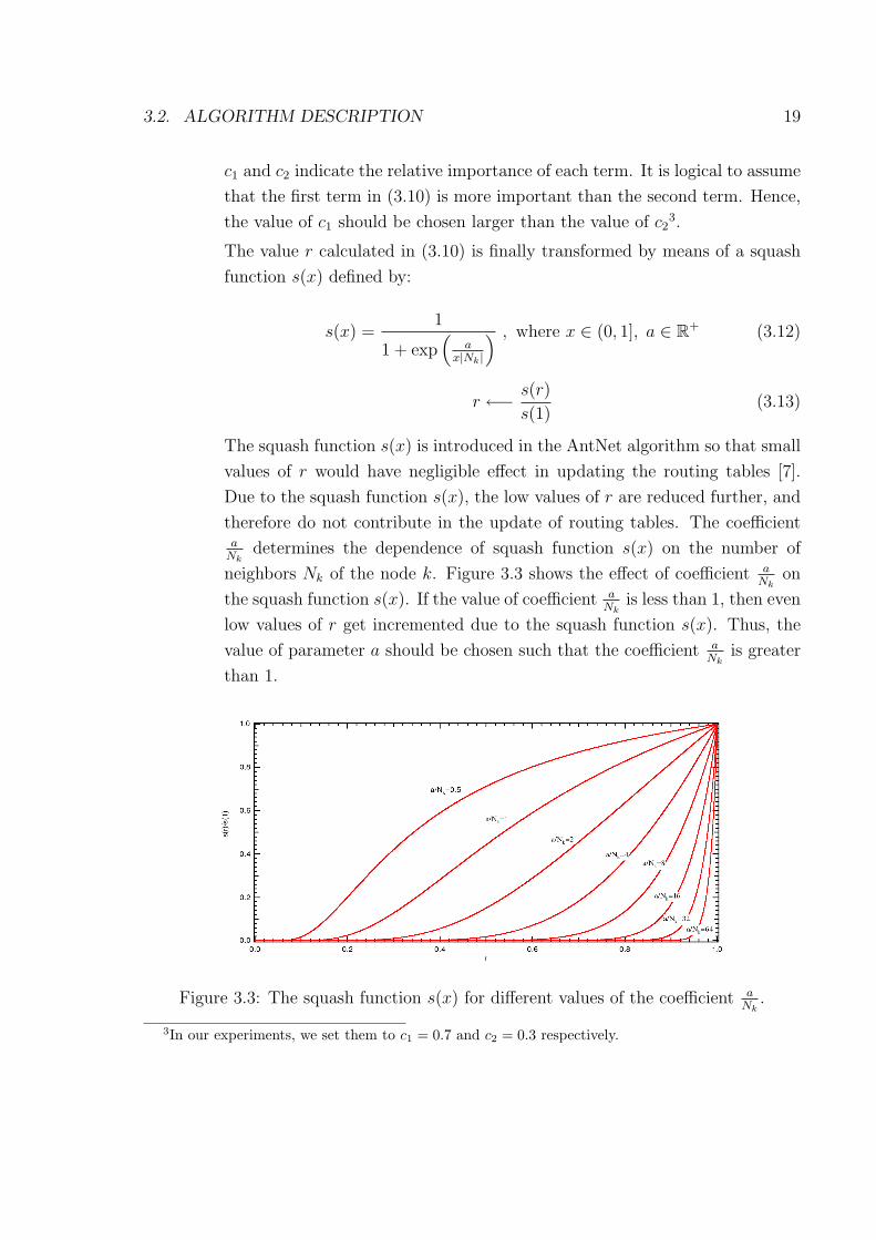
The value r calculated in (3.10) is finally transformed by means of a squash

function s(x) defined by:

s(x) =1

1 + exp(

ax|Nk|

) , where x ∈ (0, 1], a ∈ R+ (3.12)

r ←− s(r)

s(1)(3.13)

The squash function s(x) is introduced in the AntNet algorithm so that small

values of r would have negligible effect in updating the routing tables [7].

Due to the squash function s(x), the low values of r are reduced further, and

therefore do not contribute in the update of routing tables. The coefficienta

Nkdetermines the dependence of squash function s(x) on the number of

neighbors Nk of the node k. Figure 3.3 shows the effect of coefficient aNk

on

the squash function s(x). If the value of coefficient aNk

is less than 1, then even

low values of r get incremented due to the squash function s(x). Thus, the

value of parameter a should be chosen such that the coefficient aNk

is greater

than 1.

Figure 3.3: The squash function s(x) for different values of the coefficient aNk

.

3In our experiments, we set them to c1 = 0.7 and c2 = 0.3 respectively.


Data packets use different routing tables than the forward ants for travelling from

the source node to the destination node. The routing table values for data packets

are obtained by re-mapping the routing table entries used by forward ants by means

of a power function g(v) = vβ, β > 1 that emphasizes the high probability values and

reduces the lower ones. Thus, we prevent data packets from choosing links with very

low probability. In addition, data packets have a fixed time to live (TTL). If they do

not arrive at the destination within the TTL, they are dropped.

3.3 Neighbor Discovery Protocol (NDP)

We have borrowed the NDP from Zone Routing Protocol (ZRP) code [17] modifying

some parameters to adjust it to W AntNet. This protocol works in parallel with the

W AntNet algorithm and its aim is to maintain a list with available neighbors to forward

packets. It works as follows:

1. Every node broadcasts, with periodicity HELLO INTERVAL, a message to all neigh-

bors indicating that is available to forward packets.

2. Also with periodicity HELLO INTERVAL, every node checks if its neighbors are still

available. That is done by means of a timeout. Each neighbor has an associated

expire time. If the node k has not received any HELLO message from neighbor n

and current time is greater than the expire time, neighbor n is deleted from the

list. Furthermore, all entries in the routing table related to this neighbor are also

erased4.

3. Nodes are constantly listening. When a node k receive a HELLO message from node

n, it first checks if that neighbor n is already in the list. If not, the new neighbor n

is added to the list, and the routing table Tk is updated, adding an entry for every

destination d with an associated probability Pnd that is initialized to a minimum

value. If the neighbor is reliable, its probability will increase by the behavior of

the routing agents. In addition, and in all cases, the expire time is updated.

4To avoid erasing the routing information for a neighbor that is only slightly delayed, we haveincreased the number of HELLO packets allowed to be loss from 3, the most common value used inliterature, to 10. In that way, if a node that forms part of a good path is out of range just for a while,we will certainly lose some packets, but not the learning of the entire path.

Chapter 4

Simulations

To test and compare the performance of W AntNet protocol, we used the network sim-

ulator NS-2, version 2.29 [19]. The network model used in our simulation is composed

by mobile nodes and links that are considered bidirectional and wireless. Each node is

considered a communication end-point (host) and a forwarding unit (router).

In addition to NS-2, we developed a set of tools, mainly Bash scripts and AWK

filters, to post-process the output trace files generated by the simulator. Some scripts

were also written to help with the configuration and running of the multiple experiments

we have carried out.

In order to evaluate the performance, we set up multiple experiments. In each ex-

periment, W AntNet is compared with two well-known ad-hoc routing protocols, AODV

and DSR. Changes are made to either the scenario conditions or the W AntNet proto-

col parameters. In every experiment, we run a NS-2 simulation for each protocol and

different scenarios, in a similar way as [6]. The exact environment and parameters will

be discussed in 4.1.

As stated by [25] and [26], MANET simulation studies are not well prepared, and

their results are not reliable. The problem is that making a realistic scenario is difficult,

and we cannot know how complicated factors will affect our protocol. Thus, we have

started with very simple scenarios, trying to obtain similar results from other papers,

like [6] or [21]. We have changed parameters carefully to obtain results as realistic as

possible.

21

22 CHAPTER 4. SIMULATIONS

4.1 Simulation environment

In this section we will describe the procedure followed in any experiment and which tools

and programs do we use. The steps followed are:

1. Settings configuration.

2. Protocol simulation for each scenario.

3. Simulation results postprocessing.

• Extract plotable data from the trace file obtained by simulation.

• Compress trace file to save space space.

• Average results for all scenarios.

4. Display results in a graphical way.

4.1.1 Experiment Setup

The following Bash scripts have been developed to help with the simulations:

Configure experiment The script config-experiment.sh creates a folder tree and

a template config file. This file should be edited to set all the parameters of the

experiment:

$config-experiment.sh [experiment]

$vim [experiment]/config

All the parameters and settings are self-explained in the config file and will be

discussed later in this section.

Copy experiment settings If a similar experiment has to be run, one can use the

script copy-experiment.sh, which copy the movement and traffic patterns and

configuration file from the experiment passed as first argument to the second one.

Then, it asks the user to change whatever needed. Usage:

$copy-experiment.sh [source experiment] [new experiment]

4.1. SIMULATION ENVIRONMENT 23

Settings

The settings defined in the configuration file are the following:

DESCRIPTION Text explaining what we are testing on this particular experiment.

It will be printed, in addition to the results, on the plots generated by the graphical

program used. This text also contains the value of some relevant parameters that

have been changed.

i.e.

DESCRIPTION="\n\\

- Send data pkts directly if destination is a neighbor. \n\\

- IFQ=100 ETA=0.1 FA_RATE=1 pkt/s ALLOWED_HELLO_LOSS=10 pkts \n\\"

CODE REV Major revision of the NS-2 code used to simulate. That way, we can test

the effect that cause certain changes on the code. Further, we can run experiments

that use different versions of the code at the same time, without recompiling.

i.e. CODE REV="126"

PROTOCOLS Protocols we want to compare. Sometimes we will only simulate

W AntNet, and other times also AODV and DSR.

i.e. PROTOCOLS="ANTNET DSR AODV"

TESTS Tests to be performed. These can be, as explained in section 4.1.3, average

end-to-end delay (delay), packet delivery ratio (pdr), routing overhead (rov) and

hop count (hop).

i.e. TESTS="delay pdr hop"

MERGE TESTS Tests whose results should be merged. That is, write results for

every different pausetime in a single file. All tests but delay and hop can be

merged.

i.e. MERGE TESTS="pdr"

CBR SRCS List with the number of CBR sources to generate.

i.e. CBR SRCS="10 20 30"


NUM SCEN Number of random scenarios to average results. The more scenarios we

generate, the more realistic will be the results, but also more time will have to be

invested.

i.e. NUM SCEN=10

NNODES Number of mobile nodes.

i.e. NNODES=50

MAXX X dimension of topography.

i.e. MAXX=1500

MAXY Y dimension of topography.

i.e. MAXY=300

RATE Number of data packets per second sent by CBR sources.

i.e. RATE=4.0

PKTSIZE Packet size in bytes.

i.e. PKTSIZE=64

MINSPEED Minimum speed of nodes in m/s. Should be greater than zero.

i.e. MINSPEED=1

MAXSPEED Maximum speed of nodes in m/s.

i.e. MAXSPEED=20

TRAINING PERIOD Training period for W AntNet in seconds.

i.e. TRAINING PERIOD=100

SIMTIME Simulation time in seconds.

i.e. SIMTIME=900

PAUSETIMES List of simulation pause times in seconds.

i.e. PAUSETIMES="0 100 200 300 600 900"

In addition, a folder tree is created to store connection patterns, scenarios, trace files,

and plot files.


4.1.2 Running experiment

Once configured, the experiment can be started with the script run-experiment.sh. To

debug the simulation, one can add the option -gdb as:

$run-experiment -gdb [experiment]

Otherwise, one should use only:

$run-experiment.sh [experiment]

When running an experiment, the first step is to create the traffic and movement

patterns. The TCL script cbrgen.tcl is used to generate a file with the number of

connections between nodes specified by the configuration file. The traffic sources of

these connections can be either of TCP type or Constant Bit Rate (CBR) over UDP.

In all our experiments we used CBR traffic sources, the same as [6]. To generate the

movement patterns, we used a modified version of the program setdest, developed by

the Monarch Project from CMU [30]. The modified version [40] we have used provides

a steady state in that the average nodal speed consistently decreases over time.

In a movement pattern, the initial position of all nodes is randomly determined.

Then, depending on the pausetime, a destination and a random speed are calculated.

Nodes do not move during pausetime seconds. Then, they move until they arrive to the

destination point, and wait another pausetime seconds. The number of route and link

changes are stored at the end of the generated file.

If the files with those patterns already exist in the experiment folder, they are not

generated again. To overwrite them, one should first remove them and re-run the ex-

periment.

Then, for each protocol, traffic pattern, and movement pattern, a NS-2 simulation is

run. In the file manet-test.tcl are described the steps followed to simulate the ad hoc

routing protocols to compare:

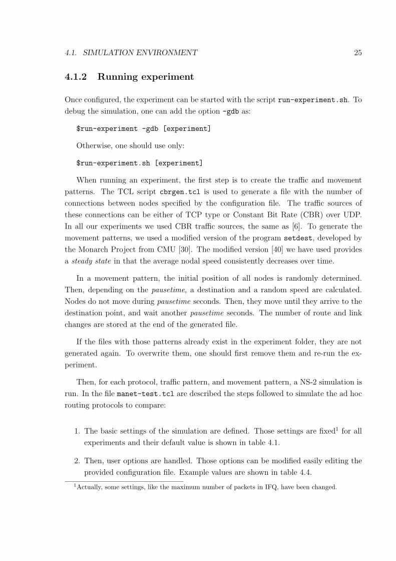
1. The basic settings of the simulation are defined. Those settings are fixed1 for all

experiments and their default value is shown in table 4.1.

2. Then, user options are handled. Those options can be modified easily editing the

provided configuration file. Example values are shown in table 4.4.

1Actually, some settings, like the maximum number of packets in IFQ, have been changed.


Channel type : WirelessChannel

Radio propagation model : TwoRayGround

Network interface type : WirelessPhy

MAC type : 802.11

MAC data rate : 2Mbps

Interface queue (IFQ) type : DropTail/PriQueue

Link layer type : LL

Antenna model : OmniAntenna

Maximum number of packets in IFQ : 100

Table 4.1: Basic settings of NS-2 simulations.

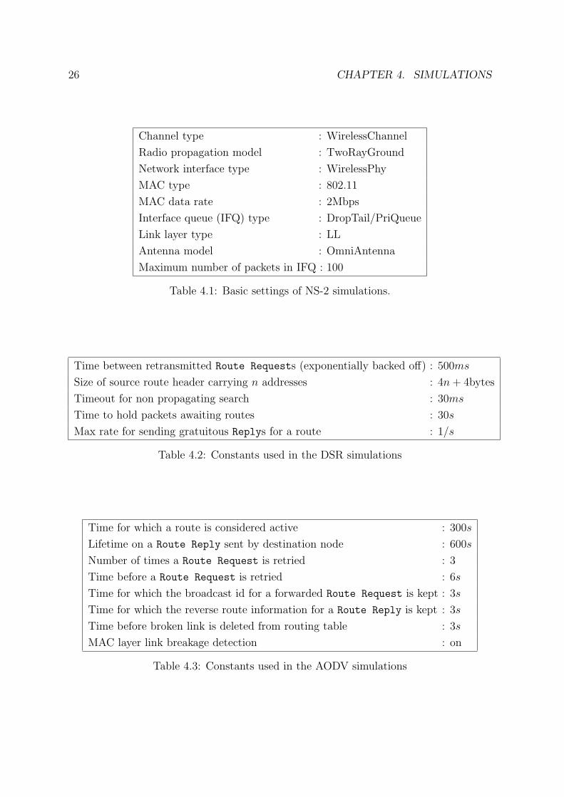
Time between retransmitted Route Requests (exponentially backed off) : 500ms

Size of source route header carrying n addresses : 4n+ 4bytes

Timeout for non propagating search : 30ms

Time to hold packets awaiting routes : 30s

Max rate for sending gratuitous Replys for a route : 1/s

Table 4.2: Constants used in the DSR simulations

Time for which a route is considered active : 300s

Lifetime on a Route Reply sent by destination node : 600s

Number of times a Route Request is retried : 3

Time before a Route Request is retried : 6s

Time for which the broadcast id for a forwarded Route Request is kept : 3s

Time for which the reverse route information for a Route Reply is kept : 3s

Time before broken link is deleted from routing table : 3s

MAC layer link breakage detection : on

Table 4.3: Constants used in the AODV simulations


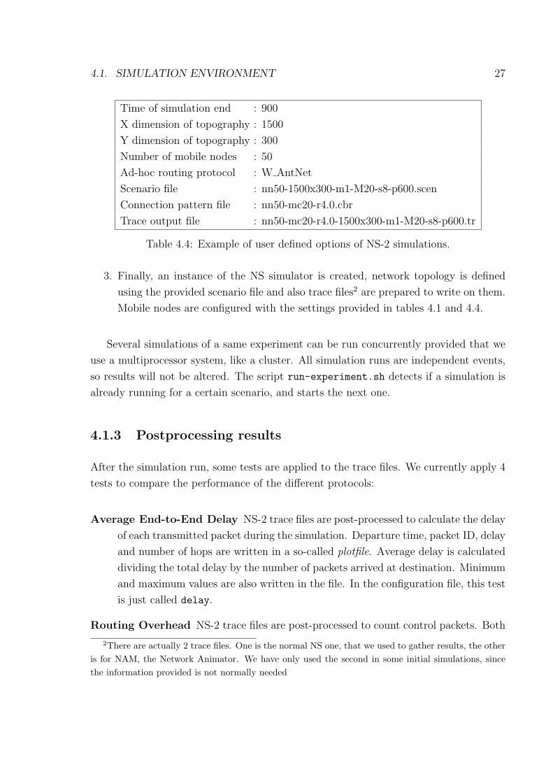
Time of simulation end : 900

X dimension of topography : 1500

Y dimension of topography : 300

Number of mobile nodes : 50

Ad-hoc routing protocol : W AntNet

Scenario file : nn50-1500x300-m1-M20-s8-p600.scen

Connection pattern file : nn50-mc20-r4.0.cbr

Trace output file : nn50-mc20-r4.0-1500x300-m1-M20-s8-p600.tr

Table 4.4: Example of user defined options of NS-2 simulations.

3. Finally, an instance of the NS simulator is created, network topology is defined

using the provided scenario file and also trace files2 are prepared to write on them.

Mobile nodes are configured with the settings provided in tables 4.1 and 4.4.

Several simulations of a same experiment can be run concurrently provided that we

use a multiprocessor system, like a cluster. All simulation runs are independent events,

so results will not be altered. The script run-experiment.sh detects if a simulation is

already running for a certain scenario, and starts the next one.

4.1.3 Postprocessing results

After the simulation run, some tests are applied to the trace files. We currently apply 4

tests to compare the performance of the different protocols:

Average End-to-End Delay NS-2 trace files are post-processed to calculate the delay

of each transmitted packet during the simulation. Departure time, packet ID, delay

and number of hops are written in a so-called plotfile. Average delay is calculated

dividing the total delay by the number of packets arrived at destination. Minimum

and maximum values are also written in the file. In the configuration file, this test

is just called delay.

Routing Overhead NS-2 trace files are post-processed to count control packets. Both

2There are actually 2 trace files. One is the normal NS one, that we used to gather results, the otheris for NAM, the Network Animator. We have only used the second in some initial simulations, sincethe information provided is not normally needed


the number of overhead packets and their size is written in a plotfile. In the

configuration file, this test is referred as rov.

Hop-Count NS-2 trace files are post-processed to count the number of packets with

a certain hop-count and the difference with the optimal hop-count. This test is

referred as hop in the configuration file.

Packet Delivery Ratio NS-2 trace files are post-processed to calculate the delivery

ratio of data packets. That is, the relation between sent packets and received

packets. This test is abbreviated in the simulation tools as pdr.

The information related to each test is extracted from the trace file and stored in a

so-called plot file. The filters are written in AWK, a programming language specially

suited to this task. We also have written some filters to average the results of different

random scenarios. All these AWK filters are located in a filters/ subfolder.

Those tests are performed just after the simulation in NS-2 for a particular scenario

has finished. Then, the trace file is compressed in gzip format to save space in the

computing system3. Once we are sure the trace files are not needed anymore, they are

manually deleted.

After all simulations of the experiment have ended, we can do the following:

Merging and averaging plots When all simulations are finished, the script average-plots.sh

can be used to merge results with different pause time in only one file, and also

to average results from different scenarios. Then, plot graphs are ready to be

displayed.

Generate command file for GNUPlot The script gen-gnuplot-commands.sh cre-

ates a file that can be loaded in GNUPlot to display graphs of interest.

Purge plots Optionally, useless plot files can be removed.

3Each tracefile use more than 100MB without compression and around 15MB otherwise. We choosethe gzip format instead of bzip2 because it requires less computing time.


4.1.4 Displaying results

To display results obtained by simulation we have used the programs GNUPlot4 and

R5. We used GNUPlot to plot the data in a easy way and R to do some statistical

processing on the data.

The plots we have included in this thesis are mainly from the tests Average end-

to-end delay and Packet Delivery Ratio. Both of them have pausetime in seconds

as X-axis. Hop-count and Routing overhead are also plotted in some experiments to

illustrate the optimal hop-count approach of W AntNet and its high route maintenance

overhead.

4See http://www.gnuplot.info/ for more information.5See http://www.r-project.org/ for more information.

http://www.gnuplot.info/

http://www.r-project.org/


4.2 Experiments

The experiments we have realized can be divided in 4 categories:

• AODV and DSR comparison to set up the simulation environment.

• Various tests using a really simple static scenario.

• Performance comparison in a wireless mobile scenario.

• Tests carried out in larger scenario.

If not stated otherwise, the scenario conditions are defined as in table 4.5. All tests

(see section 4.1.3) are applied by default.

Nodes = 50

Area = 1500x300m2

Speed = 1− 20m/s

CBR sources = 10 20 and 30

Packet size = 64bytes

Data rate = 4.0pkts/s

Pausetimes = 0 30 60 120 300 600 900 s

Table 4.5: Default scenario conditions.

4.2.1 AODV and DSR comparison

To check the correctness of our tools and tests, we first simulate a similar scenario to

[6], but comparing only AODV and DSR protocols. We set the same area, number of

nodes and movement and traffic patterns. Results obtained (see figure 4.1) were thus

similar to that paper.

4.2.2 Static scenario

The main motivation of this experiment was to test the correct behavior of our imple-

mentation. For that reason, 10 nodes were manually placed as shown in figure 4.2. The

4.2. EXPERIMENTS 31

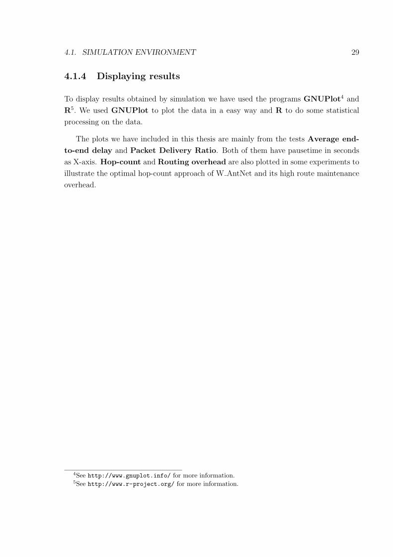
Figure 4.1: Packet Delivery Ratio converges to 100% in all cases when there is no

mobility (pausetime = 900s). DSR performance, in the other hand, decreases with the

number of active sources. Except for DSR and 30 CBR active sources, Average End-

to-End Delay is always below 0.4 seconds. Routing Overhead number of packets

decrease as pausetime increases. At pausetime = 900s (no mobility) there is no need to

send routing packets.


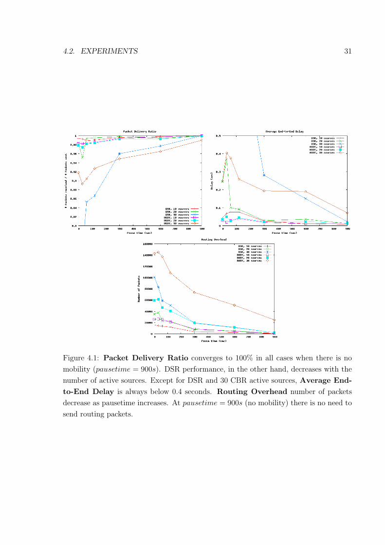
nodes did not move during the whole simulation. They remained static. In that way,

we know which neighbors has every node. In addition, traffic was set up considering 6

CBR sources and 9 concurrent connections or flows, mainly between the more distant

nodes, so they used a larger number of hops to communicate. The list of connections is

shown in table 4.6, and the list of neighbors for each node is shown in table 4.7.

Figure 4.2: The 10 wireless nodes are placed at a convenient distance of each other, so

there are enough neighbors to rely on. Radio range of 250m is also shown in the figure.

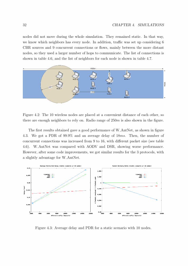
The first results obtained gave a good performance of W AntNet, as shown in figure

4.3. We got a PDR of 99.9% and an average delay of 18ms. Then, the number of

concurrent connections was increased from 9 to 16, with different packet size (see table

4.6). W AntNet was compared with AODV and DSR, showing worse performance.

However, after some code improvements, we got similar results for the 3 protocols, with

a slightly advantage for W AntNet.

Figure 4.3: Average delay and PDR for a static scenario with 10 nodes.

4.2. EXPERIMENTS 33

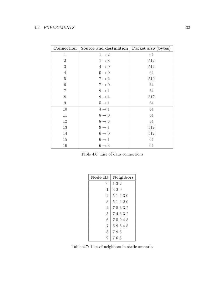
Connection Source and destination Packet size (bytes)

1 1→ 2 64

2 1→ 8 512

3 4→ 9 512

4 0→ 9 64

5 7→ 2 512

6 7→ 0 64

7 9→ 1 64

8 9→ 4 512

9 5→ 1 64

10 4→ 1 64

11 8→ 0 64

12 8→ 3 64

13 9→ 1 512

14 6→ 0 512

15 6→ 1 64

16 6→ 3 64

Table 4.6: List of data connections

Node ID Neighbors

0 1 3 2

1 3 2 0

2 5 1 4 3 0

3 5 1 4 2 0

4 7 5 6 3 2

5 7 4 6 3 2

6 7 5 9 4 8

7 5 9 6 4 8

8 7 9 6

9 7 6 8

Table 4.7: List of neighbors in static scenario


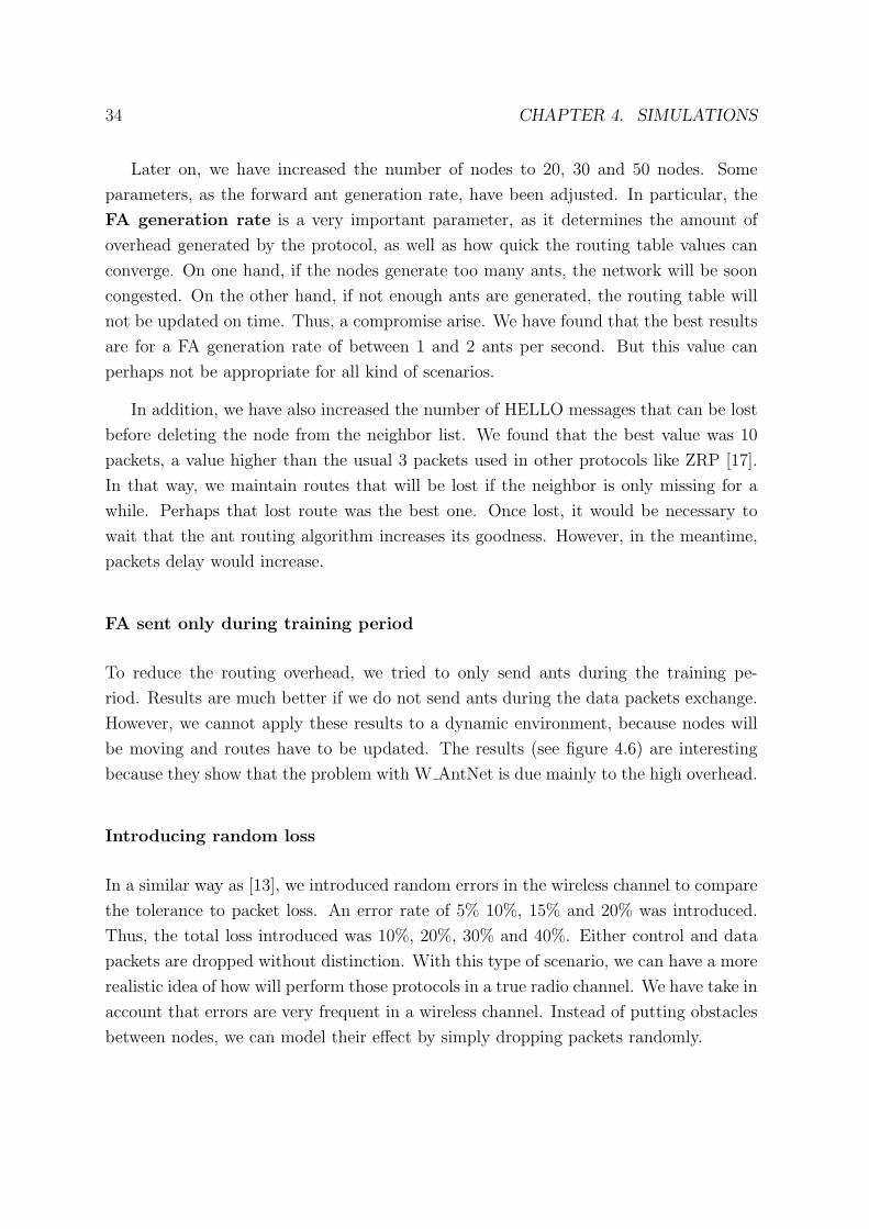
Later on, we have increased the number of nodes to 20, 30 and 50 nodes. Some

parameters, as the forward ant generation rate, have been adjusted. In particular, the

FA generation rate is a very important parameter, as it determines the amount of

overhead generated by the protocol, as well as how quick the routing table values can

converge. On one hand, if the nodes generate too many ants, the network will be soon

congested. On the other hand, if not enough ants are generated, the routing table will

not be updated on time. Thus, a compromise arise. We have found that the best results

are for a FA generation rate of between 1 and 2 ants per second. But this value can

perhaps not be appropriate for all kind of scenarios.

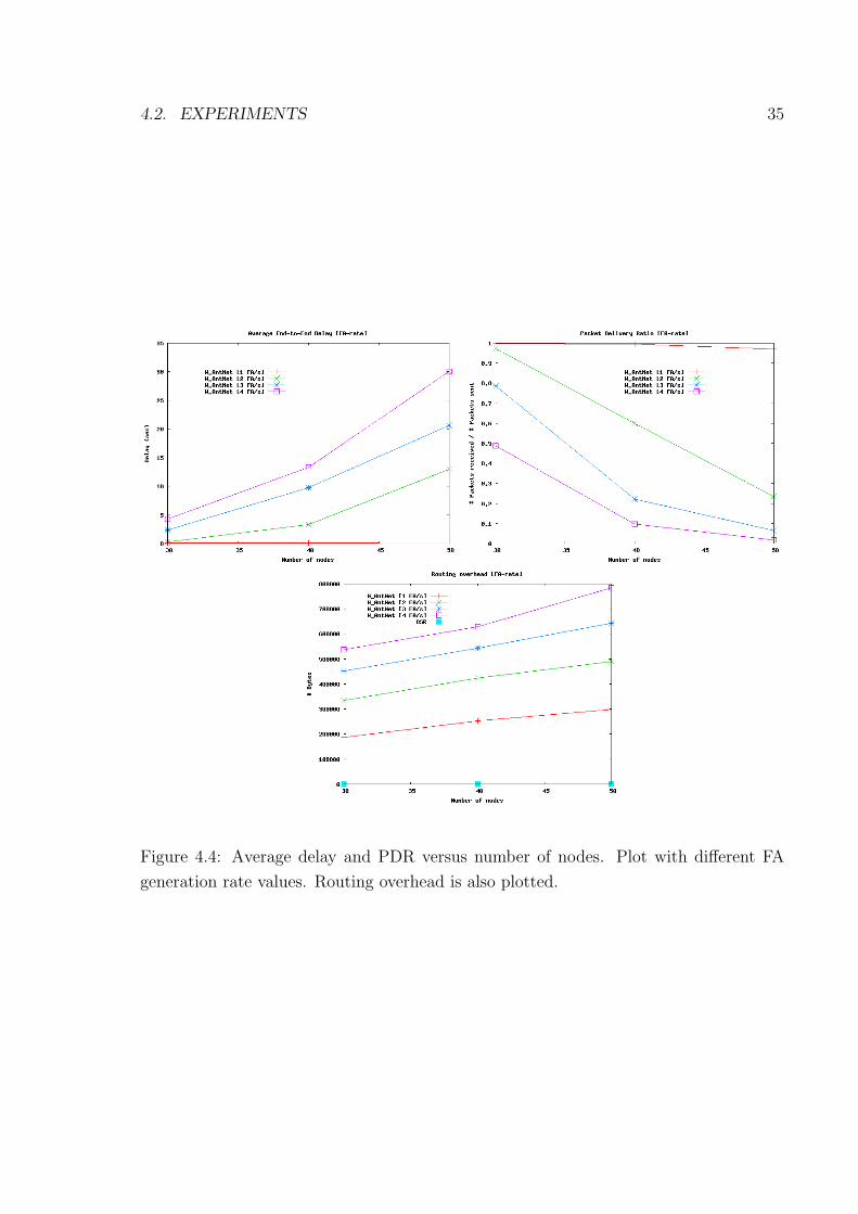
In addition, we have also increased the number of HELLO messages that can be lost

before deleting the node from the neighbor list. We found that the best value was 10

packets, a value higher than the usual 3 packets used in other protocols like ZRP [17].

In that way, we maintain routes that will be lost if the neighbor is only missing for a

while. Perhaps that lost route was the best one. Once lost, it would be necessary to

wait that the ant routing algorithm increases its goodness. However, in the meantime,

packets delay would increase.

FA sent only during training period

To reduce the routing overhead, we tried to only send ants during the training pe-

riod. Results are much better if we do not send ants during the data packets exchange.

However, we cannot apply these results to a dynamic environment, because nodes will

be moving and routes have to be updated. The results (see figure 4.6) are interesting

because they show that the problem with W AntNet is due mainly to the high overhead.

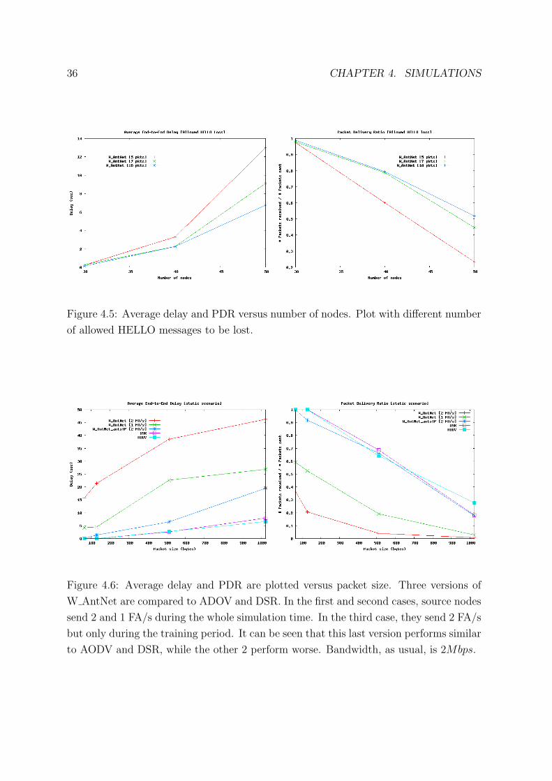
Introducing random loss

In a similar way as [13], we introduced random errors in the wireless channel to compare

the tolerance to packet loss. An error rate of 5% 10%, 15% and 20% was introduced.

Thus, the total loss introduced was 10%, 20%, 30% and 40%. Either control and data

packets are dropped without distinction. With this type of scenario, we can have a more

realistic idea of how will perform those protocols in a true radio channel. We have take in

account that errors are very frequent in a wireless channel. Instead of putting obstacles

between nodes, we can model their effect by simply dropping packets randomly.

4.2. EXPERIMENTS 35

Figure 4.4: Average delay and PDR versus number of nodes. Plot with different FA

generation rate values. Routing overhead is also plotted.


Figure 4.5: Average delay and PDR versus number of nodes. Plot with different number

of allowed HELLO messages to be lost.

Figure 4.6: Average delay and PDR are plotted versus packet size. Three versions of

W AntNet are compared to ADOV and DSR. In the first and second cases, source nodes

send 2 and 1 FA/s during the whole simulation time. In the third case, they send 2 FA/s

but only during the training period. It can be seen that this last version performs similar

to AODV and DSR, while the other 2 perform worse. Bandwidth, as usual, is 2Mbps.

4.2. EXPERIMENTS 37

Figure 4.7: For 0% and 10% packet loss, the performance of the 3 protocols is quite the

same. However, for a 20%, W AntNet packet delivery ratio decreases strongly.

4.2.3 Mobile scenario

Once studied the performance of W AntNet in a static scenario, we have set up a dynamic

scenario with 50 mobile nodes. The movement of such nodes has been determined with

the program setdest, developed by the CMU Monarch group. In particular, we have

used a modified version by EECS, University of Michigan. The code is distributed as

part of the NS-2 software suite.

In these simulations, we have also compared a modified version of W AntNet using

lookahead. That is, when the destination node is a neighbor, instead of using the routing

table, we send packets directly to it. We proved that results are much better, as shown

in 4.8. However, even if we reduce the amount of ants generated, the algorithm performs

bad compared to the other protocols.

Changing movement pattern to pause-move periods

We modified the setdest program so nodes are static for a determined PAUSE period,

and then they change their position during a MOVE period. This behaviour is repeated

until the simulation ends. Three (3) combinations have been simulated:


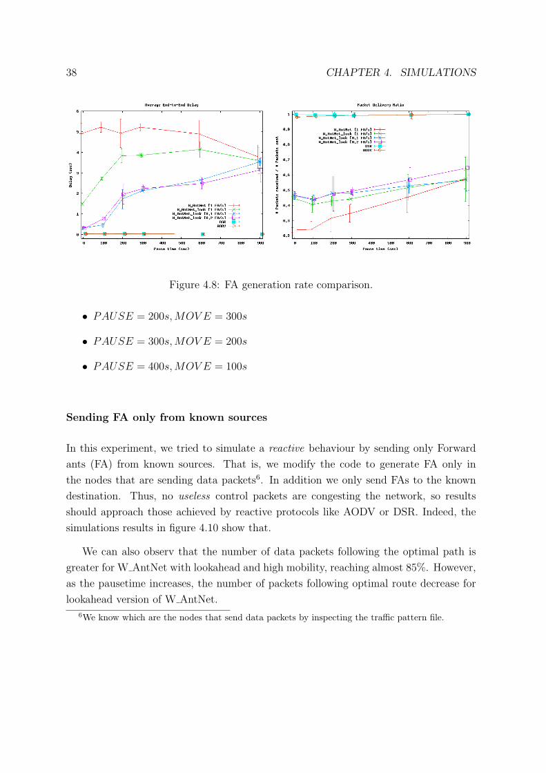
Figure 4.8: FA generation rate comparison.

• PAUSE = 200s,MOV E = 300s



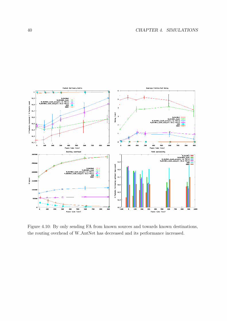
Sending FA only from known sources

In this experiment, we tried to simulate a reactive behaviour by sending only Forward

ants (FA) from known sources. That is, we modify the code to generate FA only in

the nodes that are sending data packets6. In addition we only send FAs to the known

destination. Thus, no useless control packets are congesting the network, so results

should approach those achieved by reactive protocols like AODV or DSR. Indeed, the

simulations results in figure 4.10 show that.

We can also observ that the number of data packets following the optimal path is

greater for W AntNet with lookahead and high mobility, reaching almost 85%. However,

as the pausetime increases, the number of packets following optimal route decrease for

lookahead version of W AntNet.

6We know which are the nodes that send data packets by inspecting the traffic pattern file.

4.2. EXPERIMENTS 39

Figure 4.9: We can observe that when pause period (400s) is longer than move period

(200s), packet delivery ratio is higher. That is due to the fact that the algorithm has

more time to converge and find a stable route.

4.2.4 Large scenario

In this experiment, the behavior of the 3 protocols has been tested in a large area. This

area is a square7 of 2km× 2km. The same amount of nodes has been conserved. Thus,

fewer neighbors (around 3), per node have been available. Performance should be worst

for all of them. The question is which protocol manages better this adverse scenario.

Like the others experiments, 50 nodes have been placed randomly and are moving

during simulations. Version 2 of the program ”setdest”, developed by CMU Monarch

and modified by EECS, University of Michigan, has been used to choose destination and

speed. Traffic has been set up considering CBR sources that generate 20 flows with an

offered load:

• 64bytes/pkt× 4pkt/s× 600s× 20flows = 3000kB

In general, we observe (see figure 4.11) that delay is higher when continuous motion

is applied than when nodes are static. However, packet delivery ratio is better. That

7We change the rectangular area to a square one for the same reasons as [21]. To not discriminateone direction of motion and not limit the number of hops.


Figure 4.10: By only sending FA from known sources and towards known destinations,

the routing overhead of W AntNet has decreased and its performance increased.

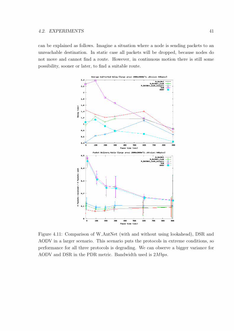
4.2. EXPERIMENTS 41

can be explained as follows. Imagine a situation where a node is sending packets to an

unreachable destination. In static case all packets will be dropped, because nodes do

not move and cannot find a route. However, in continuous motion there is still some

possibility, sooner or later, to find a suitable route.

Figure 4.11: Comparison of W AntNet (with and without using lookahead), DSR and

AODV in a larger scenario. This scenario puts the protocols in extreme conditions, so

performance for all three protocols is degrading. We can observe a bigger variance for

AODV and DSR in the PDR metric. Bandwidth used is 2Mbps.


Chapter 5

Conclusions and Future Work

5.1 Conclusions

The performance of W AntNet is comparable to the shortest path algorithm for static

topology but is dependent on the buffer size at the nodes. Since forward ants share the

same queue as data packets in W AntNet, a high ant generation rate leads to congestion

in the network. This causes W AntNet to perform poorly compared to AODV and DSR

when the size of the buffer is small. Under dynamic topology, a significant amount

of packets in W AntNet end up in loops. Hence, with mobility, the performance of

W AntNet deteriorates in comparison to AODV and DSR that are loop-free.

Furthermore, a high overhead is created by sending ants to discover paths on a

proactive way. This large overhead reduces significantly W AntNet performance. Con-

trol packets use space in the node queues, so both control and data packets are dropped.

If we reduce the generation rate of ants, then overhead is reduced. However, routing ta-

bles are not accurate enough. Using ants in a reactive way, as some protocols do [14, 15],

does not add significant improvement over other on-demand protocols, like AODV.

The use of proactive protocols for routing in ad-hoc networks is not recommended,

as shown in other simulation reports [21, 6]. A reactive approach should be done instead

of the proactive one used in this thesis. Some simulations at the end with flooding

techniques indicated that betters results can be achieved in this way.

43

44 CHAPTER 5. CONCLUSIONS AND FUTURE WORK

5.2 Recommendations for Future Work

Though ad-hoc networks are currently studied, more research has to be done to deploy

this technology in a large scale to the market. Not only about routing issues, but also

about security risks, social acceptance, and selfishness. If a user declines to route packets

for other hosts, and he only wants to use the network as transport for himself, other

hosts will not get service. Research should be done to avoid this. Furthermore, security

risks should be taken in account. For instance, a host, like a laptop or a PDA, can be

compromised by malware; thus affecting communications between nodes. Due to the

distributed routing, a node failure will not be critical, but has to be studied.

We think that perhaps AODV, already implemented in the Linux kernel [31], is a

great candidate to act as a routing agent. However, real experiments should be done

with real laptops and PDAs devices. Further simulations could also be done using

another simulator. Both OPNET [33] and QualNet [37] are good candidates and have

commercial support.

Appendix A

Resum

Ant routing es un nou esquema d’enrutament inspirat en el comportament de les formigues

o altres insectes socials. Les formigues reals son capaces de trobar el camı mes curt a una

font de menjar just seguint el rastre d’una substancia quımica anomenada feromona, la

qual es depositada per altres formigues. El rastre es veu reforcat cada vegada que passa

una formiga. I si el camı no s’utilitza amb frequencia, la feromona s’acaba evaporant. En

ant routing, les formigues (paquets de control) recullen informacio sobre les condicions

de la xarxa i son utilitzades per actualitzar i mantenir les taules d’enrutament.

El balanceig de carrega de les rutes utilitzat en ant routing s’ha provat satisfactoriament

en xarxes fixes. Aixo, juntament amb la creixent popularitat de de les xarxes ad hoc

sense fils, ens ha donat la idea de d’adaptar ant routing per a aquestes xarxes mobils i

determinar si es eficient o no. Una versio d’aquest protocol d’enrutament s’ha implemen-

tat per teballar amb el simulador de xarxes NS-2. Llavors s’ha realitzat una comparacio

de prestacions amb dos altres protocols d’enrutament ad hoc, AODV i DSR. Els resul-

tats mostren que l’overhead degut al manteniment de rutes es alt, de tal manera que

el rendiment es degrada i es inferior a AODV i DSR. No obstant, s’haurien de realitzar

mes simulacions en un altre entorn abans de rebutjar aquest esquema d’enrutament per

a xarxes sense fils ad hoc.

45

46 APPENDIX A. RESUM

A.1 Introduccio

Les xarxes mobils ad-hoc (MANETs) son xarxes auto organitzades, on no se necessita

de cap node central o infrastructura fixa. Cada node actua com a destı i enrutador de

paquets alhora. Aixo permet un suport multi-hop on dos nodes, encara que no estiguin

dins el mateix rang radio, poden comunicar-se.

L’enrutament en MANETs es difıcil per una serie de raons:

• Els nodes es mouen aleatoriament, de manera que la topologia de xarxa pot canviar

rapidament i de forma impredictible.

• Els enllacos radio, ja siguin uni o bidireccionals, tenen menor capacitat que enllacos

fixos. A mes, els efectes adversos de fading, renou, interferencies, etc. del canal

radio disminueixen encara mes aquesta capacitat. Aixo fa que la congestio sigui

mes aviat la norma que no pas l’excepcio en xarxes sense fils.

• Els nodes tenen energia limitada per l’us de bateries. Aixı que un dels criteris

d’optimitzavcio es la conservacio d’energia.

• Les xarxes poden ser grans, amb centenars o milers de nodes. Per tant, l’escalabilitat

es un altre factor que ens afectara.

S’han proposat diversos protocols (veure taula 1.1), que es poden classificar en re-

actius o proactius segons la manera de gestionar les taules d’enrutament. Els protocols

proactius escanegen la xarxa periodicament per crear i mantenir rutes des de i cap a tots

els nodes. Fins i tot si no hi ha connexions. D’aquesta manera, sempre hi ha una ruta

disponible. Els reactius, tambe anomenats on-demand, en canvi, nomes estableixen una

ruta si hi ha paquets per enviar. Aixı s’estalvia amplada de banda i es redueix overhead.

L’algoritme d’enrutament basat en el comportament de formigues que s’estudia en

aquesta tesi es una aplicacio de l’anomenada swarm intelligence. La SI intenta resoldre

problemes d’optimitzacio estatics i dinamics utilitzant agents cooperatius que es comu-

niquen entre ells modificant el seu entorn. Aquest comportament es similar al que fan

les colonies de formigues, abelles i altres insectes. Un protocol que utiliza aquestes idees

per resoldre el problema d’enrutament a xarxes fixes es AntNet [7]. AntNet ofereix,

en xarxes fixes, un rendiment superior a OSPF, Bellman-Ford, l’algoritme Q-R i Q-R

predictiu.

A.2. DESCRIPCIO I IMPLEMENTACIO DE L’ALGORITME 47

En xarxes ad-hoc, alguns protocols utilitzen ant routing, com ara Probabilistic Emer-

gent Routing Algorithm (PERA) [3], Ant Agents for Hybrid Multipath Routing (An-

tHocNet) [14] o Ant-Colony Based Routing Algorithm (ARA) [15]. El protocol que

s’implementa en aquesta tesi s’anomena W AntNet, i es una derivacio directe de AntNet.

A.2 Descripcio i implementacio de l’algoritme

A W AntNet, podem distingir 2 tipus de paquets: dades i control. Els paquets de

control poden ser forward ant (FA), backward ant (BA) o paquets per descobrir els

nostres veinats (NCP). A mes, cada node consta de dues estructures de dades: una

taula d’enrutament basada en probabilitats i un registre d’estadıstiques de trafic. Els

paquets de dades i FAs utilitzen la mateixa cua de baixa prioritat. En canvi, els paquets

BA es guarden en una cua d’alta prioritat.

El protocol consta basicament de les seguents passes:

1. A intervals regulars, cada node envia una FA a una determinada destinacio.

2. Cada node visitat i el temps de partida son guardats a la pila de la FA.

3. El seguent bot es tria a cada node de forma uniforme o segons les probabilitats de

la taula d’enrutament depenent de si ja hem visitat el node o no.

4. Si es detecta un cicle, la memoria del cicle es buida. I si es molt llarg, s’elimina la

FA completament per no desbaratar les estadıstiques.

5. Quan la FA arriba al seu destı, es genera una BA que recorre el camı en sentit

invers, actualitzant les taules d’enrutament i estadıstiques de cada node. S’escull

la ruta amb menor retard.

De forma independent i complementaria, es generen periodicament missatges HELLO

per descobrir possibles veinats.

Per implementar W AntNet s’ha utilitzat el simulador de xarxes NS-2 [19] degut

a la seva popularitat i perque ja tenia implementats els protocols amb els que voliem

comparar W AntNet. S’ha programat amb C++ i TCL orientat a objectes.

48 APPENDIX A. RESUM

A.3 Simulacions i resultats

Els experiments que hem realitzat s’han basat en [6], en un escenari de 1500×300m2, on

50 nodes es mouen a una velocitat de entre 1 i 20 m/s aleatoriament durant 900s. Per

provar distints tipus de mobilitat, s’han establert pauses entre els moviments dels nodes

de 0, 50, 100, 200, 300 600 i 900 segons. Una pausa de 0 segons representa mobilitat

continua i 900 segons representen un escenari estatic. Per a mes informacio sobre els

parametres utilitzats vegeu les taules 4.1 i 4.4.

Els experiments s’han realitzat primer en un escenari simple i estatic i llavors en un

ambient mobil. Els resultats mes destacats son:

• La frequencia de generacio de FA s’ha de triar amb cura, ja que determina la

quantitat d’overhead. Si es massa alt, la xarxa es congestiona, i si es massa baix,

les taules no convergeixen.

• W AntNet es comporta millor en situacions de poca mobilitat.

• Si les FA nomes s’envien a destinacions conegudes, el rendiment augmenta.

• Enviar els paquets directament als nodes veinats (lookahead), tambe disminueix el

retard.

• En general, el rendiment dels protocols sota demanda AODV i DSR es superior al

de W AntNet.

Per tant, futurs projectes s’haurien d’encaminar a adaptar ant routing a un esquema

reactiu en lloc de proactiu, per tal de reduir l’overhead i congestio de les cues.

Bibliography

[1] Lokesh Bajaj, Mineo Takai, Rajat Ahuja, Rajive Bagrodia, and Mario Gerla. Glo-

mosim: A scalable network simulation environment. Technical Report 990027, 13,

1999.

[2] Benjamın Baran. Improved antnet routing. SIGCOMM Comput. Commun. Rev.,

31(2 supplement):42–48, 2001.

[3] J. Baras and H. Mehta. A Probabilistic Emergent Routing Algorithm for Mobile

Ad hoc Networks (PERA), 2003.

[4] Dimitri Bertsekas and Robert Gallager. Data Networks; second edition. Prentice

Hall, 1992. BER d 92:1.

[5] Josh Broch, David B. Johnsona, and David A. Maltz. The Dynamic Source Rout-

ing Protocol for Mobile Ad Hoc Networks (DSR). Internet-draft, IETF MANET

Working Group, March 1998. Expired.

[6] Josh Broch, David A. Maltz, David B. Johnson, Yih-Chun Hu, and Jorjeta

Jetcheva. A Performance Comparison of Multi-Hop Wireless Ad Hoc Network

Routing Protocols. In Mobile Computing and Networking, pages 85–97, 1998.

http://citeseer.nj.nec.com/broch98performance.html.

[7] Gianni Di Caro and Marco Dorigo. AntNet: Distributed Stigmergetic Control for

Communications Networks. Journal of Artificial Intelligence Research, 9:317–365,

1998. http://citeseer.nj.nec.com/dicaro98antnet.html.

[8] Ching-Chuan Chiang, Hsiao-Kuang Wu, Winston Liu, and Mario Gerla. Routing

in Clustered Multihop, Mobile Wireless Networks with Fading Channel. In IEEE

Singapore International Conference on Networks, SICON’97, April 16-17, 1997,

Singapore, pages 197–211. IEEE, IEEE, April 1997.

49

http://citeseer.nj.nec.com/broch98performance.html

http://citeseer.nj.nec.com/dicaro98antnet.html

50 BIBLIOGRAPHY

[9] S. Corson and J. Macker. RFC 2501: Mobile Ad Hoc Networking (MANET):

Routing Protocol Performance Issues and Evaluation Considerations, January 1999.

Status: INFORMATIONAL., http://www.ietf.org/rfc/rfc2501.txt.

[10] Eoin Curran. Reinforcement learning for routing in ad-hoc networks. Master’s

thesis, University of Dublin, Trinity College, September 2003. http://www.maths.

tcd.ie/∼currane/swarm/.

[11] UCLA Computer Science Department. Global Mobile Information System Simula-

tor (GloMoSim). Software Package, 1999. http://pcl.cs.ucla.edu/projects/

glomosim/.

[12] Marco Dorigo and Gianni Di Caro. The Ant Colony Optimization (ACO) Meta-

Heuristic. In David Corne, Marco Dorigo, and Fred Glover, editors, New Ideas

in Optimization, pages 11–32. McGraw-Hill, London, 1999. http://citeseer.nj.

nec.com/article/dorigo99ant.html.

[13] J. Dowling, E. Curran, R. Cunningham, and V. Cahill. Using feedback in collabo-

rative reinforcement learning to adaptively optimize manet routing. Systems, Man

and Cybernetics, Part A, IEEE Transactions on, 35(3):360–372, 2005.

[14] Frederick Ducatelle, Gianni Di Caro, and Luca Maria Gambardella. Ant Agents for

Hybrid Multipath Routing in Mobile Ad Hoc Networks. In WONS, pages 44–53,

2005.

[15] M. Gunes, U. Sorges, and I. Bouazzi. ARA – the ant-colony based routing algorithm

for MANETs, 2002.

[16] Mesut Gunes and Otto Spaniol. Ant-routing-algorithm for mobile multi-hop ad-hoc

networks. pages 120–138, 2003.

[17] Zygmunt J. Haas and Marc R. Pearlman. The Zone Routing Protocol (ZRP) for

Ad Hoc Networks, 2000.

[18] John Heidemann, Nirupama Bulusu, Jeremy Elson, Chalermek Intanagonwiwat,

Kun chan Lan, Ya Xu, Wei Ye, Deborah Estrin, Ramesh Govindan, and John

Heidemann. Effects of Detail in Wireless Network Simulation. submitted to SCS

Communication Networks and Distributed Systems Modeling and Simulation Con-

ference, September 2000.

http://www.ietf.org/rfc/rfc2501.txt

http://www.maths.tcd.ie/~currane/swarm/

http://www.maths.tcd.ie/~currane/swarm/

http://pcl.cs.ucla.edu/projects/glomosim/

http://pcl.cs.ucla.edu/projects/glomosim/

http://citeseer.nj.nec.com/article/dorigo99ant.html

http://citeseer.nj.nec.com/article/dorigo99ant.html

BIBLIOGRAPHY 51

[19] Information Sciences Institute. NS-2 network simulator. Software Package, 2003.

http://www.isi.edu/nsnam/ns/.

[20] P. Jacquet, P. Muhlethaler, T. Clausen, A. Laouiti, A. Qayyum, and L. Viennot.

Optimized link state routing protocol for ad hoc networks. In Proceedings of the

5th IEEE Multi Topic Conference (INMIC 2001), 2001.

[21] Per Johansson, Tony Larsson, Nicklas Hedman, Bartosz Mielczarek, and Mikael

Degermark. Scenario-Based Performance Analysis of Routing Protocols for Mobile

ad-hoc Networks. In MOBICOM, pages 195–206, 1999.

[22] David B Johnson and David A Maltz. Dynamic Source Routing in Ad Hoc Wireless

Networks. In Imielinski and Korth, editors, Mobile Computing, volume 353. Kluwer

Academic Publishers, 1996. http://citeseer.nj.nec.com/johnson96dynamic.

html.

[23] Kevin Fall. NS notes and documentation, 2000. http://www.isi.edu/nsnam/ns/

doc/.

[24] Young-Bae Ko and Nitin H. Vaidya. Location-aided routing (LAR) in mobile ad

hoc networks. Wirel. Netw., 6(4):307–321, 2000.

[25] David Kotz, Calvin Newport, and Chip Elliott. The mistaken axioms of wireless-

network research. Technical Report TR2003-467, Dept. of Computer Science, Dart-

mouth College, July 2003.

[26] Stuart Kurkowski, Tracy Camp, and Michael Colagrosso. Manet simulation studies:

the incredibles. SIGMOBILE Mob. Comput. Commun. Rev., 9(4):50–61, 2005.

[27] Z. Liu, M. Kwiatkowska, and C. Constantinou. A biologically inspired optimisation

to AODV routing protocol. pages 106–111, December 2004.

[28] P. Van Mieghem. Data Communications Networking. Techne Press, 2006.

[29] Radovan Milosevic. Ant routing for mobile ad-hoc networks. Master’s thesis, Fac-

ulty of Information Technologies and Systems, Network Architectures and Services,

August 2003.

[30] CMU Monarch. The CMU Monarch Project’s Wireless and Mobility Extensions to

NS, 1998. http://citeseer.nj.nec.com/180061.html.

http://www.isi.edu/nsnam/ns/

http://citeseer.nj.nec.com/johnson96dynamic.html

http://citeseer.nj.nec.com/johnson96dynamic.html

http://www.isi.edu/nsnam/ns/doc/

http://www.isi.edu/nsnam/ns/doc/

http://citeseer.nj.nec.com/180061.html

52 BIBLIOGRAPHY

[31] National Institute of Standards and Technology (NIST). Kernel AODV. Software

Package, 2006. http://w3.antd.nist.gov/wctg/aodv kernel/.

[32] Valery Naumov and Thomas Gross. Scalability of routing methods in ad hoc net-

works. Perform. Eval., 62(1-4):193–209, 2005.

[33] Inc OPNET Technologies. OPNET wireless network modeling and simulation. Soft-

ware Package, 2006. http://www.opnet.com/.

[34] Vincent D. Park and M. Scott Corson. A Highly Adaptive Distributed Routing

Algorithm for Mobile Wireless Networks. In INFOCOM (3), pages 1405–1413,

1997.

[35] C. Perkins. Ad Hoc On Demand Distance Vector (AODV) Routing, 1997. http:

//citeseer.nj.nec.com/article/perkins99ad.html.

[36] Charles Perkins and Pravin Bhagwat. Highly Dynamic Destination-Sequenced

Distance-Vector Routing (DSDV) for Mobile Computers. In ACM SIGCOMM’94

Conference on Communications Architectures, Protocols and Applications, pages

234–244, 1994.

[37] Scalable Network Technologies. QualNet network simulator. Software Package,

2006. http://www.scalable-networks.com/.

[38] Subir Kumar Sarkar T.G. Basavaraju and C Puttamadappa. Impact of mac layer

on the performance of routing protocols in mobile ad hoc networks. International

Journal of Information Technology, 3(4):237–244, 2006.

[39] Otto Wittner. Ant-like mobile agents, December 2005.

[40] Jungkeun Yoon, Mingyan Liu, and Brian Noble. Random Waypoint Considered

Harmful. In INFOCOM, 2003.

http://w3.antd.nist.gov/wctg/aodv_kernel/

http://www.opnet.com/

http://citeseer.nj.nec.com/article/perkins99ad.html

http://citeseer.nj.nec.com/article/perkins99ad.html

http://www.scalable-networks.com/

Documents

Simulation of Ant Routing Protocol for Ad-hoc networks in … · Simulation of Ant Routing Protocol ... 2.4.3 Ant-Colony Based Routing Algorithm ... this tree is used to build the