Simulation of a Region Operating at 100%Renewable Energy

ByMohamed Ahmed Taha Shalaby

A Thesis submitted to Faculty of Engineering at Cairo University and KasselUniversity in Partial Fulfillment of the Requirements for the Degree of

Master of Science in Renewable Energy and Energy Efficiency

Under Supervision of

Eng. Rishabh Saxena Dr. John Sievers Prof. Mohamed El-Sobki Prof. Dirk DahlhausIdE-Kassel IdE-Kassel Cairo University Kassel University

Cairo University, EgyptKassel University, Germany

March 27, 2013

Simulation of a Region Operating at 100%Renewable Energy

ByMohamed Ahmed Taha Shalaby

A Thesis submitted to Faculty of Engineering at Cairo University and KasselUniversity in Partial Fulfillment of the Requirements for the Degree of

Master of Science in Renewable Energy and Energy Efficiency

Approved by the Examining Committee:

Prof. Mohamed El-Sobki Thesis Advisor and MemberFaculty of Engineering, Cairo University Signature

Prof. Dirk Dahlhaus MemberChair of communication laboratory, Kassel University Signature

Prof. Amr Adly MemberFaculty of Engineering, Cairo University Signature

Dr. Hani Nokraschy MemberNokraschy Engineering GmbH, Germany Signature

Cairo University, Cairo, EgyptKassel University, Kassel, Germany

March 27, 2013

ii

Declaration for the Master’s ThesisI, Mohamed Shalaby, hereby affirm that the master thesis at hand is my own written

work and that I have used no other sources and aids others than those indicated. Onlythe sources cited have been used. Those parts which are direct quotes or paraphrases areidentified as such.

Kassel, Germany March 27, 2013Place Date Signature

iv

Contents

Table of Contents v

List of Figures vii

List of Tables x

Acknowledgment xi

List of Acronyms xiii

Abstract xvi

1 Introduction 11.1 Introduction to Renewable Energy . . . . . . . . . . . . . . . . . . . . . 11.2 Reasons to shift to Renewable Energy . . . . . . . . . . . . . . . . . . . 11.3 Renewable Energy Analysis Programs . . . . . . . . . . . . . . . . . . . 2

2 Modeling Renewable Energy Generators 32.1 Photovoltaic system model . . . . . . . . . . . . . . . . . . . . . . . . . 3

2.1.1 Photovoltaic system connected to grid . . . . . . . . . . . . . . . 32.1.2 Photovoltaic system with Batteries . . . . . . . . . . . . . . . . . 9

2.2 Wind turbine model . . . . . . . . . . . . . . . . . . . . . . . . . . . . . 102.2.1 Vertical Wind Profile . . . . . . . . . . . . . . . . . . . . . . . . 102.2.2 Test wind turbine model . . . . . . . . . . . . . . . . . . . . . . 11

2.3 Bio Generator Model . . . . . . . . . . . . . . . . . . . . . . . . . . . . 122.3.1 Algorithm for the Bio Generator Model . . . . . . . . . . . . . . 12

3 Optimization Method 133.1 Motivation for Optimization Method . . . . . . . . . . . . . . . . . . . . 133.2 Introduction to the Optimization tool . . . . . . . . . . . . . . . . . . . . 133.3 Algorithm for optimization tool . . . . . . . . . . . . . . . . . . . . . . . 14

3.3.1 Percentage of Renewable Energy . . . . . . . . . . . . . . . . . . 153.3.2 Autonomy percentage . . . . . . . . . . . . . . . . . . . . . . . 153.3.3 Carbon dioxide emission . . . . . . . . . . . . . . . . . . . . . . 163.3.4 Annual income to the region . . . . . . . . . . . . . . . . . . . . 173.3.5 Investment costs . . . . . . . . . . . . . . . . . . . . . . . . . . 183.3.6 Job creation . . . . . . . . . . . . . . . . . . . . . . . . . . . . . 193.3.7 Annual Operation & Maintenance costs . . . . . . . . . . . . . . 203.3.8 Public acceptance . . . . . . . . . . . . . . . . . . . . . . . . . . 21

v

3.4 The optimum scenario . . . . . . . . . . . . . . . . . . . . . . . . . . . 223.5 Results . . . . . . . . . . . . . . . . . . . . . . . . . . . . . . . . . . . . 23

4 Case study#1: Osnabrück, Germany 254.1 Overview about Renewable Energy in Osnabrück . . . . . . . . . . . . . 254.2 Renewable Energy Potential in Osnabrück . . . . . . . . . . . . . . . . . 27

4.2.1 Photovoltaic . . . . . . . . . . . . . . . . . . . . . . . . . . . . . 274.2.2 Hydropower . . . . . . . . . . . . . . . . . . . . . . . . . . . . . 274.2.3 Biogas . . . . . . . . . . . . . . . . . . . . . . . . . . . . . . . 274.2.4 Wind . . . . . . . . . . . . . . . . . . . . . . . . . . . . . . . . 27

4.3 Electric demand for Osnabrück . . . . . . . . . . . . . . . . . . . . . . . 284.4 Load profile for Osnabrück . . . . . . . . . . . . . . . . . . . . . . . . . 294.5 Simulation load profile with renewable energy . . . . . . . . . . . . . . . 304.6 Results . . . . . . . . . . . . . . . . . . . . . . . . . . . . . . . . . . . . 30

5 Case study#2: Siwa, Egypt 335.1 Overview about Siwa electric grid . . . . . . . . . . . . . . . . . . . . . 33

5.1.1 Grid history . . . . . . . . . . . . . . . . . . . . . . . . . . . . . 335.1.2 Electric Energy . . . . . . . . . . . . . . . . . . . . . . . . . . . 335.1.3 Load Profile . . . . . . . . . . . . . . . . . . . . . . . . . . . . . 345.1.4 Electric Energy Expectation . . . . . . . . . . . . . . . . . . . . 35

5.2 Energy Efficiency Potential . . . . . . . . . . . . . . . . . . . . . . . . . 365.3 Pre-Feasibility study for replacing current street lamps by LED lamps . . 37

5.3.1 Introduction . . . . . . . . . . . . . . . . . . . . . . . . . . . . . 375.3.2 Investment costs . . . . . . . . . . . . . . . . . . . . . . . . . . 375.3.3 Running costs . . . . . . . . . . . . . . . . . . . . . . . . . . . . 375.3.4 Savings and Payback period . . . . . . . . . . . . . . . . . . . . 385.3.5 Sensitivity Analysis . . . . . . . . . . . . . . . . . . . . . . . . . 395.3.6 Strengths, Weaknesses, Opportunities and Threats (SWOT analysis) 40

5.4 Potential of Renewable Energy in Siwa . . . . . . . . . . . . . . . . . . . 415.4.1 Wind Energy . . . . . . . . . . . . . . . . . . . . . . . . . . . . 415.4.2 Bio Energy . . . . . . . . . . . . . . . . . . . . . . . . . . . . . 425.4.3 Solar Energy . . . . . . . . . . . . . . . . . . . . . . . . . . . . 42

5.5 Pre-Feasibility study for 100% Renewable Energy for Siwa . . . . . . . . 435.5.1 Introduction . . . . . . . . . . . . . . . . . . . . . . . . . . . . . 435.5.2 Key Assumptions . . . . . . . . . . . . . . . . . . . . . . . . . . 435.5.3 Renewable Energy Scenarios for Siwa . . . . . . . . . . . . . . . 435.5.4 Investment cost . . . . . . . . . . . . . . . . . . . . . . . . . . . 445.5.5 Cash Flow Analysis . . . . . . . . . . . . . . . . . . . . . . . . . 445.5.6 Savings and Payback Period . . . . . . . . . . . . . . . . . . . . 455.5.7 Sensitivity Analysis . . . . . . . . . . . . . . . . . . . . . . . . . 465.5.8 Strengths, Weaknesses, Opportunities and Threats (SWOT analysis) 50

5.6 Simulation . . . . . . . . . . . . . . . . . . . . . . . . . . . . . . . . . . 505.6.1 Monthly Energy Profile 2020 . . . . . . . . . . . . . . . . . . . . 505.6.2 Simulation load profile with renewable energy . . . . . . . . . . 515.6.3 Results . . . . . . . . . . . . . . . . . . . . . . . . . . . . . . . 51

vi

6 Conclusion, Recommendations and Future Work 536.1 Conclusion . . . . . . . . . . . . . . . . . . . . . . . . . . . . . . . . . 536.2 Recommendations . . . . . . . . . . . . . . . . . . . . . . . . . . . . . . 536.3 Future Work . . . . . . . . . . . . . . . . . . . . . . . . . . . . . . . . . 54

Reference 56

vii

viii

List of Figures

2.1 Equivalent circuit for an ideal solar cell is a current source in parallel withdiode. . . . . . . . . . . . . . . . . . . . . . . . . . . . . . . . . . . . . 3

2.2 Equivalent circuit diagram for the effective solar cell characteristic withRPV connected in series . . . . . . . . . . . . . . . . . . . . . . . . . . 4

2.3 Block diagram for the PV model with inputs IMPP , VMPP , VOC , ISC , CT ,NOCT , G, Tamb, Cap, installation year and simulation year, while PDCis output from PV model . . . . . . . . . . . . . . . . . . . . . . . . . . 6

2.4 Block diagram for the inverter model with inputs η10%, η50%, η100%, PDCand Pnominal, while ηxx% and PAC are the outputs from the inverter model 7

2.5 Different PV systems installed on the roof of Stuttgart University . . . . . 82.6 Test for PV model shows the simulated PAC by Wagner model and real

PAC for one week . . . . . . . . . . . . . . . . . . . . . . . . . . . . . . 82.7 Block diagram for the PV system with Batteries, explains the algorithm

for PV system with Batteries . . . . . . . . . . . . . . . . . . . . . . . . 92.8 Block diagram for wind model, explaining the algorithm for wind model . 112.9 Test for wind model shows the simulated PAC and power curve from

datasheet . . . . . . . . . . . . . . . . . . . . . . . . . . . . . . . . . . 112.10 Block diagram for bio model, explaining the algorithm for bio model . . . 12

3.1 Block diagram for the optimization tool. . . . . . . . . . . . . . . . . . . 143.2 4D plot for the percentage of Renewable Energy . . . . . . . . . . . . . . 153.3 4D plot for the percentage of autonomy . . . . . . . . . . . . . . . . . . 163.4 4D plot for carbon dioxide emission reduction in tonne. . . . . . . . . . . 173.5 4D plot for income to the region in Million Euros. . . . . . . . . . . . . . 183.6 4D plot for investment costs in Million Euros. . . . . . . . . . . . . . . . 193.7 4D plot shows the number of jobs created within the region. . . . . . . . 203.8 4D plot shows the annual costs for operation & maintenance in Million

Euros. . . . . . . . . . . . . . . . . . . . . . . . . . . . . . . . . . . . . 213.9 4D plot shows the public acceptance within the region. . . . . . . . . . . 223.10 4D plot shows the optimum case at 100% renewable energy. . . . . . . . 23

4.1 Renewable Energy installed in Osnabrück . . . . . . . . . . . . . . . . . 254.2 Installed renewable energy capacity for each community in Osnabrück . . 264.3 Map with Renewable energy installed in each community in Osnabrück . 264.4 The annual expected electric energy consumption and energy generated

from renewable sources from 2010 until 2050 in the county of Osnabrück 284.5 The expected hourly load profile for the county Osnabrück in 2030 . . . . 294.6 Hourly load profile for the county of Osnabrück for 48 hours and the gen-

erated power from renewable energy sources in the region . . . . . . . . . 31

ix

5.1 The monthly electric consumption for Siwa, Egypt for 2011 and 2012. . . 345.2 Hourly electric load profiles for Siwa, Egypt for one day. . . . . . . . . . 355.3 Electric energy expectation from 2013 until 2020 for Siwa, Egypt. . . . . 355.4 Old and new electric load profile after replacing the old street lamps by

new LED lamps. . . . . . . . . . . . . . . . . . . . . . . . . . . . . . . 375.5 Monthly energy consumed by street lighting in Siwa. . . . . . . . . . . . 385.6 Monthly energy costs form street lighting in Siwa. . . . . . . . . . . . . . 385.7 Sensitivity analysis for the payback period for the project by changing the

price of diesel at constant investment cost. . . . . . . . . . . . . . . . . . 395.8 Sensitivity analysis for payback period for project by changing the price

of LED lamps at constant diesel price. . . . . . . . . . . . . . . . . . . . 405.9 Wind regime map for Egypt (Wind atlas for Egypt). . . . . . . . . . . . . 415.10 Solar radiation intensity Map for Egypt (Solar atlas for Egypt). . . . . . . 425.11 The net cash flow for 100% renewable energy project in Siwa. . . . . . . 455.12 The cumulative net cash for 100% renewable energy project in Siwa. . . . 455.13 Effect of price development for PV system on NPV, at constant transmis-

sion lines cost and constant interest rate. . . . . . . . . . . . . . . . . . . 465.14 Effect of price development for transmission lines on NPV, at constant PV

system cost and constant interest rate. . . . . . . . . . . . . . . . . . . . 475.15 Effect of interest rate development on NPV, at constant PV system and

constant transmission line cost. . . . . . . . . . . . . . . . . . . . . . . . 475.16 Effect of price development for PV systems on IRR, at constant transmis-

sion lines cost and constant interest rate. . . . . . . . . . . . . . . . . . . 485.17 Effect of price development for transmission lines on IRR, at constant PV

system cost and constant interest rate. . . . . . . . . . . . . . . . . . . . 495.18 Effect of interest rate development on IRR, at constant PV system and

transmission lines cost. . . . . . . . . . . . . . . . . . . . . . . . . . . . 495.19 The expected monthly electric energy profile for Siwa in 2020. . . . . . . 515.20 The monthly imports/exports from and to Siwa region. . . . . . . . . . . 52

x

List of Tables

1.1 Energy system analysis programs. . . . . . . . . . . . . . . . . . . . . . 2

2.1 Variation of α with terrain. . . . . . . . . . . . . . . . . . . . . . . . . . 10

5.1 Investment cost of different renewable energy scenarios for Siwa. . . . . . 44

xi

AcknowledgmentFirst I would like to thanks DAAD for providing me with the scholarship and specialthanks to Ms. Bikomo and Ms. Dombret.

Many thanks as well go to my colleagues in IdE and deENet and specially my super-visors Dr. John Sievers and Rishabh Saxena, for their support to me during conduction ofthe thesis.

I would like to thank my reviewers Prof. Mohamed Elsobki and Prof. Dirk Dahlhaus.I would like to thank all REMENA team and professors in Cairo University and Kas-

sel University for their support. Moreover I would like to thank all my colleagues inRE3MENA.

Sincere thanks to my lovely parents, brother and sister for their continuously encour-agement throughout the years of my studies.

I would like to thank Eng. Ali Abdelnaby for his hospitality in Siwa and providing mywith support and data about Siwa grid.

I would like to thankUsamaMohamad andHanaKhalil for supportingmewithwritingmy master thesis in LaTeX.

I would like to thanks my friends in Kassel Mostafa Mamdouh, Amr Esbitan, YehiaFawzy and special thanks for Ahmad Talaat.

xii

List of Acronyms

α Thermal coefficient of short circuitα Exponent depends on the roughness of the surfaceηxx% Efficiency of the inverter at xx%ρ Standard air densityA Area of the wind turbineCInvBio

Investment costs for BioCInvP V

Investment costs for PVCInvW

Investment costs for WindCO&MRE

Operation & Maintenance cost for Renewable Energy technologyCsellBio

Selling price for BioCsellP V

Selling price for PVCsellW Selling price for windCf Capacity factorCp Power coefficient of wind turbineCT Temperature coefficient of powerCap Capacity of PV systemCapNewBio

New Bio capacityCapNewP V

New PV capacityCapNewW

New Wind capacityECO2Bio

Emission due to operation of Bio generatorsECO2P V

Emission due to operation of PVECO2W

Emission due to operation of wind turbineG Global irradiationI Current produced by PV moduleIMPP Maximum power point currentIph PhotocurrentISC Short circuit currentID Diode currentIo Diode saturation currentM Slope at open circuit voltageNJobBio

Number of jobs created by Bio generatorsNJobP V

Number of jobs created by PVNJobW

Number of jobs created by windPACP

AC power produced by PVPACW

AC power produced by Wind turbinePNetP W

Power produced by PV and wind subtracted from load profilePNetP W

Load Profile after subtraction of power produced by PV and wind turbinePAC AC power outputPBio Power produced by Bio generatorsPDC Output power from PV modelPLoad Load Profile

xiv

Ploss Normalized power losses in inverterPMPP0 Photovoltaic module at specific solar irradiation and temperaturePNetH PLoad − PPVPout Normalized output power to the nominal powerPPV Power by PV systemPPV Power produced by all PV systemsPSelf Normalized self-consumption for the inverterPW Power produced by all wind turbinesPARE Public acceptance for the renewable energy technologyrloss Normalized ohmic losses in inverterRPV Photovoltaic resistanceRS Series resistanceRE% Renewable Energy percentTamb Ambient temperatureTj Temperature of Photovoltaic moduleVloss Normalized voltage losses on diodes and transistors in inverterVMPP Maximum power point voltageVOC Open circuit voltageVPV Photovoltaic module voltageVT Thermal voltageipv Institute for PhotovoltaicsAC Alternating currentBMU Nature Conservation and Nuclear SafetyCO2 Carbon dioxideDAAD German Academic Exchange ServiceDC Direct CurrentGWh Gigawatt hourIdE Institut dezentrale EnergietechnologienISE Fraunhofer-Institute for Solar Energy SystemskV Kilo VoltkW KilowattkWh Kilowatt hourLED Light Emitting DiodeMW MegawattNOCT Nominal Operating Cell TemperaturePLGross

Gross load profilePLNet

Net load profilePV PhotovoltaicSOC State Of ChargeSTC Standard Test ConditionSWOT Strength, Weakness, Opportunities and ThreatsUBA Federal Environment Agency

xv

AbstractThis master thesis presents PV, wind, bio generator models to model renewable energygenerators. Those models were built on MATLAB platform. A new optimization toolis presented to calculate the optimum capacity needed to be installed in order to reach100% renewable energy with in the region. This optimization tool takes into consider-ation autonomy, costs, CO2 emission, job creation, operation & maintenance costs andpublic acceptance. The result of optimization tool is the optimum capacities from eachrenewable energy technology needed to be installed in the region to be operating at 100%renewable energy. This master thesis simulate two regions operating at 100% renewableenergy. The first region is Osnabrück, Germany, while the second region is Siwa, Egypt.The optimization tool proposed to increase the capacity of PV systems to 578 MW, windcapacity to 1842 MW and bio generators to 120 MW, so the county of Osnabrück couldoperate at 100% renewable energy. The result of optimization tool have been used to sim-ulate hour-by-hour the county gross load profile and power generated by renewable energywithin the county of Osnabrück. Energy efficiency in street lights in Siwa has been dis-cussed from the technical and economical point of view, in order to facilitate the path forrenewable energy to fulfill the load demand. Siwa region could operate at 100% renew-able energy by installing 21 MW PV systems and construct transmission lines connectingSiwa grid with Libya grid.

xvii

Chapter 1

Introduction

The Institute of decentralized Energy technologies (IdE) is currently carrying out the"100% Renewable Energy Regions" project. This project identifies, monitors and net-works regions and municipalities whose goals are to switch their energy supply in thelong run to be supplied entirely on renewable energy. There are over one hundred andthirty districts, municipalities and regional networks in Germany pursuing this goal. Theproject "100% Renewable Energy Regions" is funded by the Federal Ministry for Envi-ronment, Nature Conservation and Nuclear Safety (BMU) and the Federal EnvironmentAgency (UBA).

This Master Thesis presents a new optimization method to simulate a region operatingat 100% renewable energy. Moreover it contains two cases studies simulations one forOsnabrück, Germany and the other for Siwa, Egypt.

1.1 Introduction to Renewable EnergyRenewable Energy is defined as energy that is produced by natural resources - such assunlight, wind, rain, waves, tides and geothermal heat - that are naturally replenishedwithin a time span of a few years [1].

1.2 Reasons to shift to Renewable EnergyMany countries such as Denmark, Ireland and Japan are setting goals to switch their en-ergy supply to be working on 100% renewable energy [1, 2, 3, 4]. The main reasonsthat those countries took the decision of replacing fossil energy and nuclear energy byrenewable energy are:

• Energy Security: As the prices of fossil fuel are increasing and fossil fuel reservesare depleting, countries dependent on importing oil may face risk of supply of en-ergy [1].

• Environment: With the increase of the concentration of green house gases in theatmosphere, the temperature of earth increases, which have an effect on the humanhealth and the environment [5].

• Nuclear Energy problems: Although Nuclear Energy could produce tremendousamount of energy, it has many disadvantages like waste treatment, accidents (Cher-nobyl 1986 and Fukushima 2011), safety and high investment costs.

1

1.3 Renewable Energy Analysis ProgramsThere exist a large number of different computer programs that analyses renewable energysystems. Those programs could be categorized into two main groups. The first group isbased on aggregated annual calculations, while the second group is based on a detailedhour-by-hour simulation. In analyses of 100% renewable energy regions it is essential touse hour-by-hour simulation [1]. Table 1.1 shows different Renewable Energy analysisprograms available in the market that are based on aggregated annual calculations andones which are based on detailed hour-by-hour simulation.

Table 1.1: Energy system analysis programs.

Aggregated Annual Calculations Detailed Hour-by-Hour SimulationsEnergyBALANCE EnergyPLAN

LEAP LEAPMARKAL RAMSESPRIMES BALMORELENPEP SESAM

SIVAELWASPH2RESHOMER

IdE would like to have a deep look on the grid problems and what needs to be changedin the infrastructure of the transmission grid for the regions which would operate on 100%renewable energy. IdE had to implement a tool like the ones presented in table 1.1 intwo phases to determine the grid problems. The first phase is presented in this masterthesis, which is modeling each renewable energy technology and combining it togetherto calculate the net electric energy produced by renewable energy and subtract it fromthe electric load profile to determine the imports and exports from and to the region.Moreover this tool has a new optimization method that takes into the consideration manyaspects like autonomy, costs, CO2 emission, job creation, operation & maintenance costs,public acceptance and etc. This program is based on hour-by-hour simulation and it couldbe easily modified to work with accuracy minute-by-minute, depending on the accuracyof the meteorological data. In the second phase, which is still under development, thetool would be able to predict problems that may occur to the transmission system to theregions operating at 100% renewable energy.

Chapter 2 in this master thesis introduces the models used to build this tool, whilechapter 3 presents the new optimization method. This optimization tool is going to beused to get the optimum capacity needed to be installed in Osnabrück, Germany, which isgoing to be the first case study in thesis, which is explained in more details in chapter 4.The second case study is in Siwa, Egypt which is presented in chapter 5.

2

Chapter 2

Modeling Renewable EnergyGenerators

This chapter is going to introduce models for representing Photovoltaic (PV) system, windturbine and bio generators. The power produced by PV systems, wind turbines and biogenerators are summed up hourly and subtracted from the electric load to know the hourlyexports/imports for electricity to/from region.

2.1 Photovoltaic system modelThis section is going to present two different PV systems. The first PV system would bedirectly connected to the electric grid, while the second PV system is connected to theelectric grid with battery bank to increase the self consumption of the building.

2.1.1 Photovoltaic system connected to gridPV systems connected to the electric grid consists of PV modules connected in seriesand parallel to convert sun light to direct current (DC) and inverter that convert DC toalternating current (AC) for grid connection.

PVmodule consists of number of solar cells connected in series. The solar cell has thesame physical structure as a diode. It consists of a p- and n- doped semiconductor, whichcould be represented by a diode. A current source in parallel with the diode representsthe current produced by an ideal solar cell when light is applied on it. Figure 2.1 showsthe equivalent circuit for an ideal solar cell.

IPh

ID, V

Figure 2.1: Equivalent circuit for an ideal solar cell is a current source in parallel withdiode.

3

Wagner presented the equivalent circuit for the effective solar cell characteristic byadding fictitious PV resistance RPV . RPV is different than the series resistance RS in thesingle diode model [6, 7]. It is fictitious, as the value for it could be a negative or positive.As negative resistance doesn’t exist in reality, the component in the equivalent circuitdiagram can’t be an ohmic resistance. Figure 2.2 shows the equivalent circuit diagram forthe effective solar cell characteristic.

IPh

ID, VD

RPV I

RVPV

Figure 2.2: Equivalent circuit diagram for the effective solar cell characteristic with RPV

connected in series

The value for the current I produced by the PV module could be calculated by equa-tion 2.1

I = IPh −

ID︷ ︸︸ ︷Io

(exp

(VPV + IRPV

VT

)− 1

)(2.1)

Where IPh is the photocurrent produced by current source, Io is the diode saturationcurrent, VT is the thermal voltage and ID is the diode current. While the voltage acrossthe PV module VPV is

VPV = VT ln(IPh − I + Io

Io

)− IRPV (2.2)

The Value for RPV is defined by equation 2.3

RPV = −M ISCIMPP

+ VMPP

IMPP

(1 − ISC

IMPP

)(2.3)

Where ISC is short circuit current, IMPP is the maximum power point current, VMPP

maximum power point voltage at standard test condition (STC) andM is the slope at opencircuit voltage VOC and it could be calculated by equation 2.4

M = VOCISC

(K1

IMPPVMPP

ISCVOC+K2

VMPP

VOC+K3

IMPP

ISC+K4

)(2.4)

Where K are constants defined in the following vector

K =

−5.4116.4503.417

−4.422

(2.5)

The photocurrent IPh produced by current source could be calculated by equation 2.6

IPh = ISCG (1 + α (Tj − 25))1000 (2.6)

4

where G is the global irradiation in watt on 1 m2, α is the thermal coefficient of shortcircuit and Tj is the temperature of PV module. The thermal voltage VT is calculated byequation 2.7

VT = −(M +RPV )ISC (2.7)

The diode saturation current Io is calculated by equation 2.8

Io = ISC exp(

−VOCVT

)(2.8)

The temperature for the PV module Tj is calculated by equation 2.9

Tj = Tamb + (NOCT − 25) G

800 (2.9)

where Tamb is the ambient temperature of the air and NOCT is nominal operating celltemperature.

The maximum power point PMPP0 for PV module at specific solar irradiation andtemperature is calculated based on Wagner model by equations 2.10, 2.11, 2.12 [7].

PMPP0 = VMPP0IMPP0 (2.10)

VMPP0 = VMPP

1 + CT (Tj − 25)+VT298

Tj + 273 ln(

G

1000

)−IMPPRPV

(G

1000 − 1)

(2.11)

IMPP0 = IMPPG

1000 (2.12)

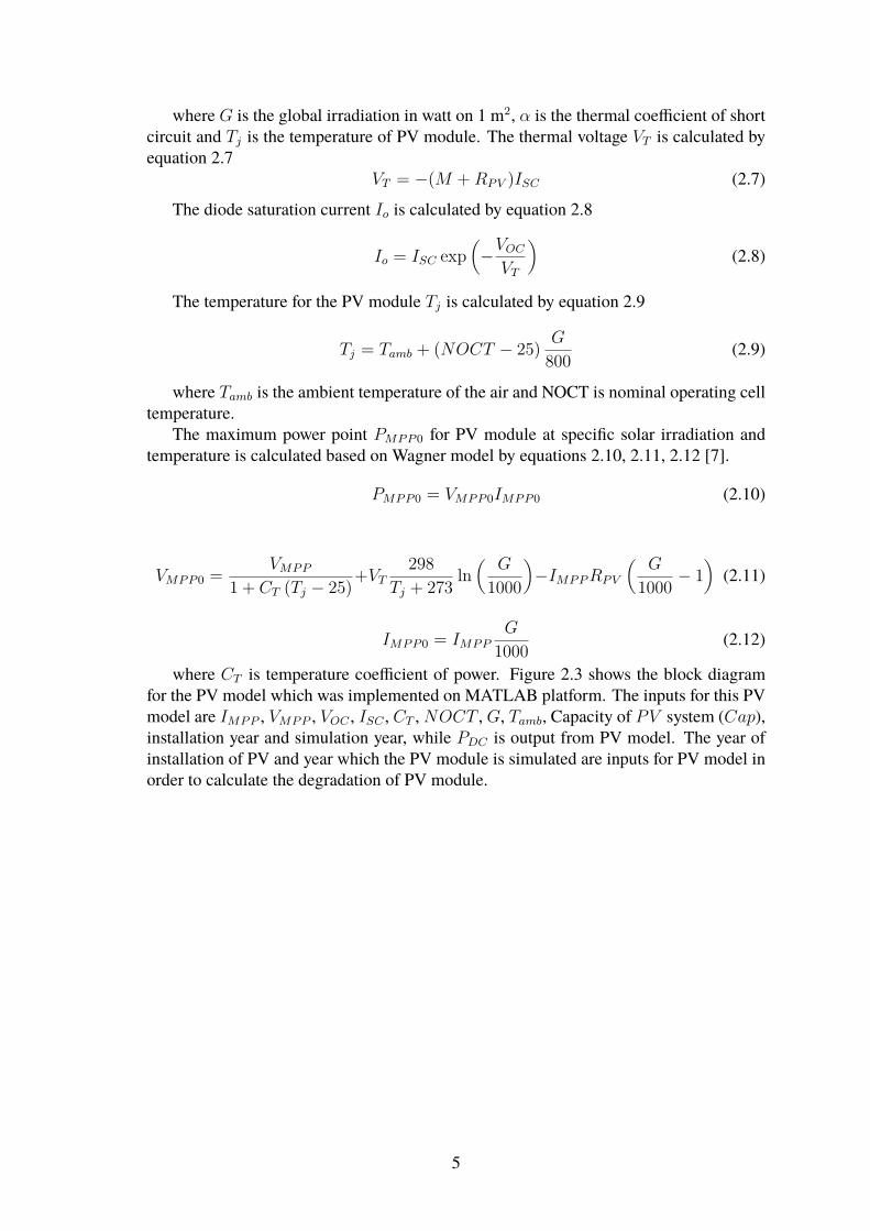
where CT is temperature coefficient of power. Figure 2.3 shows the block diagramfor the PV model which was implemented on MATLAB platform. The inputs for this PVmodel are IMPP , VMPP , VOC , ISC , CT ,NOCT ,G, Tamb, Capacity of PV system (Cap),installation year and simulation year, while PDC is output from PV model. The year ofinstallation of PV and year which the PV module is simulated are inputs for PV model inorder to calculate the degradation of PV module.

5

IMPPl[A]

VMPPl[V]

Ctl[k-1

]Gl[W/m

2]

Meteonorm

Tjl[oC]

DatasheetlforlPVlmodule

PDCl[W]

Ml[V/A]

NOCTl[oC]DatasheetlforlPVlmodule

Tamb [oC]

MeteonormIMPPl[A]

VMPPl[V]

ISCl[A]

VOCl[V]

DatasheetlforlPVlmodule

RPVl[V/A]IMPPl[A]

ISCl[A]DatasheetlforlPVlmodule

VTl[V]

Installationlyear

Simulationllyear

PVlModel

Capl[kW]

Figure 2.3: Block diagram for the PV model with inputs IMPP , VMPP , VOC , ISC , CT ,NOCT , G, Tamb, Cap, installation year and simulation year, while PDC is output fromPV model

Photovoltaic Inverter model

H. Schmidt and D. U. Sauer from Fraunhofer-Institute for Solar Energy Systems (ISE)presented a model for the efficiency curve of inverters [8]. This inverter model requiresparameters which could be easily determined from the datasheet of the inverter. Theefficiency for the inverter could be described by equation 2.13

η = − 1 + vloss2rlossPin

+

√√√√ (1 + vloss)2

(2rlossPin)2 + Pin − PselfrlossP 2

in

(2.13)

Where PSelf represents normalized self-consumption for the inverter, vloss represents nor-malized voltage losses on diodes and transistors and rloss normalized ohmic losses. Thenormalized power losses Ploss is described by equations 2.14, 2.15.

Ploss = Pin − Pout (2.14)

Ploss = Pself + vlossPout + rlossP2out (2.15)

Pout represents the normalized output power to the nominal power. Equation 2.15 showsthat the losses increase with the square of the power output. By substituting with the abovetwo equation, Pout could be calculated by solving the following quadratic equation 2.16.

rlossP2out + Pout(vloss + 1) − Pin + Pself = 0 (2.16)

The parameters vloss, Pself and rloss could be easily calculated from the power curve fromthe datasheet of the inverter by knowing the efficiencies of the inverter at 10%, 50% and100% of the nominal power.

6

vloss is calculated by equation 2.17.

vloss = −43

1η100%

+ 3312

1η50%

− 512

1η10%

(2.17)

Pself is calculated by equation 2.18.

Pself = − 199

1η100%

+ 1099

1η10%

− 111 (2.18)

rloss is calculated by equation 2.19.

rloss = 10099

1η100%

− 1099

1η10%

− 1011 (2.19)

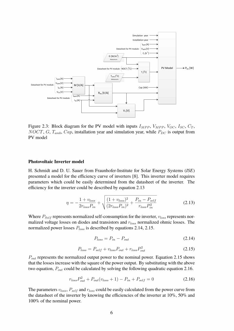
Figure 2.4 shows a block diagram for the inverter model. The inputs for the invertermodel are efficiency of the inverter at 10%, 50% and 100% of the nominal power and theinput DC power PDC . While the outputs for the inverter model are AC power PAC andefficiency of the inverter ηxx%.

Figure 2.4: Block diagram for the inverter model with inputs η10%, η50%, η100%, PDC andPnominal, while ηxx% and PAC are the outputs from the inverter model

Test Photovoltaic model

PV model have been tested by comparing PAC output from the PV model with real PVsystem installed on top of the university building in Stuttgart. Figure 2.5 shows a figure forthe different PV systems installed on the roof of Stuttgart University. Schubert andWursterfrom Institute for Photovoltaics (ipv), Stuttgart University provided us with data for globalradiation (G), temperature of PV module and AC power from PV system (PAC) for oneof the PV systems for one week. This PV system consists of 5 modules of Suntechnics(STM200FM) connected in series. The PV module array is connected with SMA (SunnyBoy 1100) inverter.

7

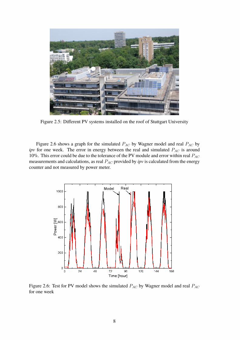
Figure 2.5: Different PV systems installed on the roof of Stuttgart University

Figure 2.6 shows a graph for the simulated PAC by Wagner model and real PAC byipv for one week. The error in energy between the real and simulated PAC is around10%. This error could be due to the tolerance of the PV module and error within real PACmeasurements and calculations, as real PAC provided by ipv is calculated from the energycounter and not measured by power meter.

Figure 2.6: Test for PV model shows the simulated PAC by Wagner model and real PACfor one week

8

2.1.2 Photovoltaic system with Batteries

The prices of installation of PV modules have been decreasing dramatically in the lastfew years, in addition to that the prices for feed in tariff is decreasing too [9]. Grid par-ity has been reached in Germany, therefore people have become more interested in self-consumption of their own energy generated from PV systems. As PV systems producepower only during day time, while the home/company consumes power during the entireday, so batteries are needed to cover the evening demand.

This section is presenting PV system with batteries as a backup. Figure 2.7 shows ablock diagram for the PV system with batteries. The PV system with batteries uses thePV model presented in the previous section. The load profile for home/company PLoad isfed into the model, so that the load profile PLoad is subtracted from PAC produced by PVmodel. The result from the subtraction is named PNetH . Based on the value of PNetH thealgorithm would take a decision.

If PNetH is positive it means that there is enough power to supply the load at that timeand the extra power should be used either to charge the batteries or to feed in the extrapower into the electric grid based on the state of charge (SOC) of the batteries.

In case PNetH is negative it means that there is not enough power to supply the load, sopower has to be discharged from the batteries or taken from the electric grid, dependingon SOC of the batteries.

The inputs for the PV model with batteries are load profile PLoad, capacity of batteriesand the same inputs for the PV model, while the outputs are self-consumption-percent,PNetH and SOC. The maximum allowed SOC is 100%, while the minimum allowed SOCis 50%, to protect the life cycle of the batteries.

Figure 2.7: Block diagram for the PV system with Batteries, explains the algorithm forPV system with Batteries

9

2.2 Wind turbine modelThis section presents a model for 3−bladed horizontal axis wind turbine. The inputsparameters for this model are wind speeds v (ho), height of measuring equipment (ho),hub height of wind turbine (h), roughness of the surface (α), swept area of the windturbine (A) and the power coefficient of wind turbine (Cp).

2.2.1 Vertical Wind ProfileThe wind turbines are installed at high hub heights, while wind measurement equipmentare installed at 10 ˜ 50 meter high. The wind speed at the hub height of the wind turbinecould be estimated by the vertical wind profile equation 2.20 [10]. Table 2.1 shows thevariation of α with terrain.

v(h) = v(ho)(h

ho

)α(2.20)

Table 2.1: Variation of α with terrain.

Type of terrain αCalm open sea 0.104Snow 0.1Rough pasture 0.112Crops 0.131Scattered trees 0.188Forest 0.213Suburbs 0.257City centers 0.289

Figure 2.8 shows a block diagram for wind model, explaining the algorithm of thewind turbine model. If v(h) is higher than cut-out wind speed, that means that the windturbine, should be switched off to protect it and PAC is zero, while if v(h) is lower thanthe cut-in speed that means there isn’t enough power in the wind to rotate the wind turbineand PAC is zero.

If v(h) is between cut-in and cut-out wind speed that means that wind turbine is pro-ducing and PAC produced by the wind turbine could be calculated by equation 2.21 [11].

PAC = 12ρ (v(h))3 CpA (2.21)

Where ρ is the standard air density 1.225 kg/m3. Cp and A are available in the datasheetof the wind turbine manufacture.

10

Figure 2.8: Block diagram for wind model, explaining the algorithm for wind model

2.2.2 Test wind turbine modelFigure 2.9 shows 2 curves for PAC by ENERCON E-126 wind turbine. The dashed blackcurve is power curve that is given by the datasheet of the manufacturer. The second curvein red is PAC simulated by wind model.

Figure 2.9: Test for wind model shows the simulated PAC and power curve from datasheet

11

2.3 Bio Generator ModelThis section presents the bio generatormodel and an algorithm for it. The input parametersfor the bio generator model are load profile after subtracting the power produced by PVand wind (PNetP W

) and the bio capacities which are going to be simulated, while theoutput for the bio generator model are load profile after subtraction of power produced byPV, wind and power produced by the bio generator model.

2.3.1 Algorithm for the Bio Generator ModelThe gross load profile (PLoad) and power produced by the simulated PV systems with inthe region (PACP

) for one year are loaded and subtracted from each other. The resultof this subtraction is called PNetP . The power produced by wind turbines in the region(PACW

) is subtracted from PNetP and the result is named PNetP W.

The bio generator model operates each bio generator 15 hours within 30 hours. Itwould check the highest peaks within 30 hours. Then it would check if there is any Biogenerator that could fulfill the load demand by itself, if yes then this generator would gointo operation, if not then the Bio model would operate more than one generator to fulfillthe load demand (Priority to bigger generators as they are more efficient). After the loadhas been covered by the one or more Bio generators, the Bio model would check the nexthighest peak, until it reaches with it to minimum for 30 hours. Then it would go to checkthe next 30 hours until the year is done.

The outputs for the Bio model are PNetP W Bwhich is load profile minus power pro-

duced by PV, wind and Bio generators and PACBiowhich is the power produced by the

Bio generators.

Figure 2.10: Block diagram for bio model, explaining the algorithm for bio model

12

Chapter 3

Optimization Method

3.1 Motivation for Optimization Method100% renewable energy projects presented in [1, 3, 4, 12] are propose four to six scenarioswith different combination of technology and comparing between those different scenar-ios on the basis of economic factors, carbon dioxide (CO2) emission, imports/exports ofenergy etc. On the other hand, there could be infinite combination of different renew-able energy technologies with which a region could reach 100% renewable energy. Thischapter is going to introduce a new optimization tool that scans the space of differentrenewable energy technologies starting from current installed capacity to the maximumpotential that could be installed in the region, until it reaches 100% renewable energy andpresents an optimal result for each of the following factors: autonomy, costs, CO2 emis-sion, job creation, operation & maintenance costs and public acceptance. The MATLABplatform was used for developing the optimization method. This optimization tool findsthe optimum technology combination based on weighted sum matrices.

3.2 Introduction to the Optimization toolFigure 3.1 shows the block diagram of the algorithm for the optimization tool. The toolconsists of the PV, Wind and Bio models presented in chapter 2. It starts by the currentinstalled capacity in the region and calculates the hourly power produced by each tech-nology and subtracts it from the load profile. The energy produced by renewable energyis calculated as a percentage from the total electric load demand. If the percentage ofrenewable energy is less than 100%, then the tool would recalculate with higher capacityinstalled for PV, Wind and Bio until 100% renewable energy is achieved in the region.

13

PV model

Wind model

PPV

PW

Current State à Max. Potential

Capacity (kW)

+ - Bio modelPBio

Autonomy

Load profile for region %

Σ O&MCost

Bio Energy

Wind Energy

PV Energy

Million €

CO2 Emission

Tons CO2

Income Million €

Current State à Max. Potential

Capacity (kW)

Current State à Max. Potential

Capacity (kW)

PPV

PW

PNetPW

PNetPWB

Job creation

No. Jobs

Investment costs

Million €

Public acceptance

%

PLoad

PLoad

Renewable Energy Percent

%

Figure 3.1: Block diagram for the optimization tool.

3.3 Algorithm for optimization tool

First the algorithm calculates the hourly power produced by PV systems (PPV ) withinthe region, based on the current installed capacity. Then, it calculates the hourly powerproduced by wind turbines (PW ) within the region based on the current installed capacityand sums it with the power produced by PV systems. The summed power from PPV andPW are subtracted from the hourly growth load profile for the region and the result ofthis subtraction named PNetP W

. PNetP Wis one of the inputs for the Bio model. The Bio

model chooses the load peaks, when there isn’t enough power from PV and wind to supplythe load demand and operates the Bio generators. The outputs from the Bio generatormodel are hourly power produced by Bio generators (PBio) in the region and load profileafter subtracting power generated by PV, wind and Bio generators. The energy for eachrenewable energy technology is calculated by summing the hourly power generated forthe whole year.

When 100% renewable energy is reached, the tool would calculate the autonomy, CO2emission, investment costs, number of jobs created, operation & maintenance costs andincome for the region.

14

3.3.1 Percentage of Renewable EnergyThe tool calculates the percentage of renewable energy RE% for this region by equa-tion 3.1, which is the sum of energy produced by PV systems, wind turbines and Bio gen-erators, divided by the total energy demand for this region, multiplied by 100 to presentit as a percentage.

RE% =

8760∑1PPV +

8760∑1PW +

8760∑1PBio

8760∑1PLoad

× 100 (3.1)

The tool presents the percentage of renewable energy in a 4D plot. Figure 3.2 showsthe 4D plot for the percentage of renewable energy. The x-, y-, z-axes represent the capac-ities installed for PV, Wind and Bio respectively. While the color of the surface representsthe fourth dimension, which is the percentage of renewable energy for the given inputcombination. The surface in figure 3.2 represents the 100% renewable energy surfaceand higher1, which means that any point below this surface denotes a scenario less than100% renewable energy, while any point above this surface means it is more than 100%renewable energy. The color column on the right hand side represents the color code forthe percentage of renewable energy.

100200

300400

500600

700

200

400

600

800

1000

1200

1400

1600

1800

2000

0

200

400

600

PV capacity [MW]

4D plot for Renewable Energy Percent

Wind capacity [MW]

Bio

cap

acity

[MW

]

101

102

103

104

105

106Percentage ofRenewableEnergy [%]

Figure 3.2: 4D plot for the percentage of Renewable Energy

3.3.2 Autonomy percentageThe autonomy could be defined as the percentage of energy that, is produced and con-sumed locally without exports and imports. The inputs for the autonomy block are PLoadand PNetP W B

. The autonomy block calculates the percentage of demand which hasn’t1The reason that there are more than 100% renewable energy on the surface, is the big steps taken by

renewable energy capacities, decreasing the steps would lead to increase the computation time for 4D plot

15

been directly supplied by renewable energy produced within the region and subtracts itfrom 100, to calculate the percentage of energy that has been produced and consumedlocally without exports and imports.

Figure 3.3 shows a 100% renewable energy surface. The color of the surface representsthe percentage of autonomy for each combination. The color column on the right handside represents the color code for the percentage of autonomy. It can be noticed fromthe plot that there is a direct correlation between the capacity of Bio generators and theautonomy, as Bio generators are flexible renewable energy sources which operate basedon the demand, while PV and wind energy production is dependent on meteorologicalconditions.

100200

300400

500600

700

200

400

600

800

1000

1200

1400

1600

1800

2000

0

200

400

600

PV capacity [MW]

4D plot for Autonomy

Wind capacity [MW]

Bio

cap

acity

[MW

]

60

65

70

75

80

85

90

Autonomy[%]

Figure 3.3: 4D plot for the percentage of autonomy

3.3.3 Carbon dioxide emissionThe carbon dioxide emission is one of the key elements that make the regions take thedecision of shifting to renewable energy. The carbon dioxide (CO2) emission block cal-culates the amount of carbon dioxide emission based on the amount of energy producedby each renewable energy technology. The carbon dioxide emission for PV is 94 g/kWhel(ECO2P V

), wind is 32 g/kWhel (ECO2W) and Bio generators 640 g/kWhel (ECO2Bio

) [13].

ECO2T otal=(ECO2P V

8760∑1PPV

)+(ECO2W

8760∑1PW

)+(ECO2W

8760∑1PBio

)(3.2)

Figure 3.4 shows the plot with the 100% renewable energy surface. The color ofthe surface represents the carbon dioxide emission reduction for each combination. Thecolor column on the right hand side represents the color code for carbon dioxide emissionreduction. It can be noticed that the more the Bio generators installed the higher theemission, while the more PV and wind are installed the less the CO2 emission.

16

100200

300400

500600

700

200

400

600

800

1000

1200

1400

1600

1800

2000

0

200

400

600

4D plot for carbon dioxide emission

PV capacity [MW]

Wind capacity [MW]

Bio

cap

acity

[MW

]

4

5

6

7

8

9

10

11

x 105

Carbon dioxideemission[Tonne]

Figure 3.4: 4D plot for carbon dioxide emission reduction in tonne.

3.3.4 Annual income to the regionOne of the advantages of a 100% renewable energy project to the region is the valuecreated by the income from selling renewable energy electricity to the region and theregions around it. The selling price for PV (CsellP V

) is set at 0.18 €/kWhele, wind (CsellW )0.07 €/kWhele and Bio (CsellBio

) 0.05 €/kWhele [14]. The income block would calculatethe annual income to the region by equation 3.3.

Income =(CsellP V

8760∑1PPV

)+(CsellW

8760∑1PW

)+(CsellBio

8760∑1PBio

)(3.3)

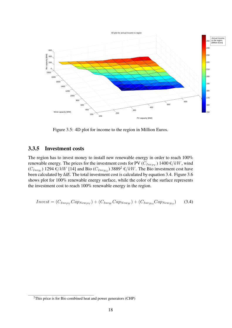
Figure 3.5 shows plot for 100% renewable energy surface, while the color of the sur-face represents the annual income to the region, due to selling electricity into the regionand the regions around it. It is noticed from the figure 3.5 that the higher the installedwind capacity the higher the annual income to the region.

17

100

200

300

400

500

600

700

200

400

600

800

1000

1200

1400

1600

1800

2000

0

200

400

600

PV capacity [MW]

4D plot for annual income to region

Wind capacity [MW]

Bio

cap

acity

[MW

]

150

160

170

180

190

200

210

220

230

240

250Annual incometo the region[Million Euro]

Figure 3.5: 4D plot for income to the region in Million Euros.

3.3.5 Investment costsThe region has to invest money to install new renewable energy in order to reach 100%renewable energy. The prices for the investment costs for PV (CInvP V

) 1400 €/kW , wind(CInvW

) 1294 €/kW [14] and Bio (CInvBio) 38892 €/kW . The Bio investment cost have

been calculated by IdE. The total investment cost is calculated by equation 3.4. Figure 3.6shows plot for 100% renewable energy surface, while the color of the surface representsthe investment cost to reach 100% renewable energy in the region.

Invest = (CInvP VCapNewP V

) + (CInvWCapNewW

) + (CInvBioCapNewBio

) (3.4)

2This price is for Bio combined heat and power generators (CHP)

18

100200

300400

500600

700

200

400

600

800

1000

1200

1400

1600

1800

2000

0

100

200

300

400

500

4D plot for investment costs

PV capacity [MW]

Wind capacity [MW]

Bio

cap

acity

[MW

]

3000

4000

5000

6000

7000

8000

Investmentcosts[Million Euro]

Figure 3.6: 4D plot for investment costs in Million Euros.

3.3.6 Job creationThe number of jobs created in the region is one of the key elements for the value creationwithin the region. The number of jobs created for installing PV (NJobP V

) is 30 Job/MW ,wind (NJobW

) is 22 Job/MW and Bio (NJobBio) is 15 Job/MW [15]. The total number

of jobs created is calculated by equation 3.5. Figure 3.7 shows plot for 100% renewableenergy surface, while the color of the surface represents the number of jobs created.

NJobT otal= (NJobP V

CapNewP V) + (NJobW

CapNewW) + (NJobBio

CapNewBio) (3.5)

19

100200

300400

500600

700

200

400

600

800

1000

1200

1400

1600

1800

2000

0

200

400

600

4D plot for number of jobs created

PV capacity [MW]

Wind capacity [MW]

Bio

cap

acity

[MW

]

3.4

3.6

3.8

4

4.2

4.4

4.6

4.8

x 104

Number of jobs created

Figure 3.7: 4D plot shows the number of jobs created within the region.

3.3.7 Annual Operation & Maintenance costsThe annual operation & maintenance costs (CO&MT otal

) are calculated for PV and windbased on the capacity installed. The annual cost for operation & maintenance for PV(CO&MP V

) is 34.75 €/MW and wind (CO&MW) is 47.32 €/MW , while the annual opera-

tion & maintenance costs for Bio is based on the annual generated energy, as operation &maintenance costs for Bio generators depends more on operation hours for the generator.The annual cost for operation & maintenance for Bio (CO&MBio

) is 2.74 €/MWh [14].The total annual operation & maintenance costs are calculated by equation 3.6.

CO&MT otal= (CO&MP V

CapPV ) + (CO&MWCapW ) +

(CO&MBio

8760∑1PBio

)(3.6)

20

100

200

300

400

500

600

700

200

400

600

800

1000

1200

1400

1600

1800

2000

0

200

400

600

PV capacity [MW]

4D plot for Operation & Maintenance cost

Wind capacity [MW]

Bio

cap

acity

[MW

]

0.04

0.05

0.06

0.07

0.08

0.09

0.1

Annual operation &Maintenancecost [Million Euro]

Figure 3.8: 4D plot shows the annual costs for operation & maintenance in Million Euros.

3.3.8 Public acceptanceThe public acceptance (PA) is defined by grading system (from 0 to 5) for each renewableenergy technology. Zero means that this technology isn’t accepted within the region, onthe other hand five means that this technology is highly accepted within the region. Basedon this grading system the new installed capacity from each technology in kW would bemultiplied by its grade. Then all the results of multiplicities grades would be summed upto give a figure for the public acceptance within the region. The matrix for public accep-tance is normalized by dividing by highest element in the matrix. It has been assumedthat the public acceptance for PV (PAPV ) is 3, wind (PAW ) is 3 and Bio (PABio) is 5.Equation 3.7 shows how the elements of the matrix for public acceptance is calculated.Figure 3.9 shows a 4D plot for the public acceptance within the region. The color codefor public acceptance is form 0 to 1. Zero means it isn’t accepted, while one means that itis highly accepted.

PA = (PAPVCapNewP V) + (PAWCapNewW

) + (PABioCapNewBio) (3.7)

21

100200

300400

500600

700

200

400

600

800

1000

1200

1400

1600

1800

2000

0

200

400

600

PV capacity [MW]

4D plot for Public acceptance

Wind capacity [MW]

Bio

cap

acity

[MW

]

0.1

0.2

0.3

0.4

0.5

0.6

0.7

0.8

0.9

1PublicAcceptance

Figure 3.9: 4D plot shows the public acceptance within the region.

3.4 The optimum scenarioThe question when choosing the capacity that needed to be installed to reach 100% re-newable energy, which is the technology is the most optimum and from which point ofview? Is it the investment costs, CO2 emission · · · etc?

The product of each of the 4D plots in section 3.3 is a matrix, the elements of thematrix could be normalized, by dividing it by the maximum element within the matrix, sothat all the elements of the matrix is between 0 and 1. The optimum matrix is calculatedby the below equation, whereC represents the coefficients of the matrices and it is a scalarvalue. The coefficients are graded from 0 to 5 based on how important this parameter tothe region, for example if this region suffers from high carbon dioxide emission, then thisregion would give CCO2 , 5, while on the other hand if this region have low unemploy-ment, then CJob could be set to 0 or 1. Equation 3.8 shows how the optimum matrix iscalculated. The optimum matrix is normalized by dividing all the elements of the matrixby the maximum element in the matrix. The color code for optimum is form 0 to 1. Onemeans that it is the optimum scenario.

22

X11 . . . Xi1... . . .

...X1j . . . Xij

Optimum

= CAuto.

A11 . . . Ai1... . . .

...A1j . . . Aij

Auto

− CCO2

ECO211

. . . ECO2i1... . . ....

ECO21j. . . ECO2ij

CO2

+CIncome

Inc11 . . . Inci1

... . . ....

Inc1j . . . Incij

Income

+ CJob

Njob11 . . . Njobi1... . . .

...Njob1j

. . . Njobij

Job

−CInvest

Inv11 . . . Invi1

... . . ....

Inv1j . . . Invij

Invest

− CO&M

CO&M11 . . . CO&M i1

... . . ....

CO&M1j. . . CO&M ij

O&M

+CPublic

PA11 . . . PAi1

... . . ....

PA1j . . . PAij

Public

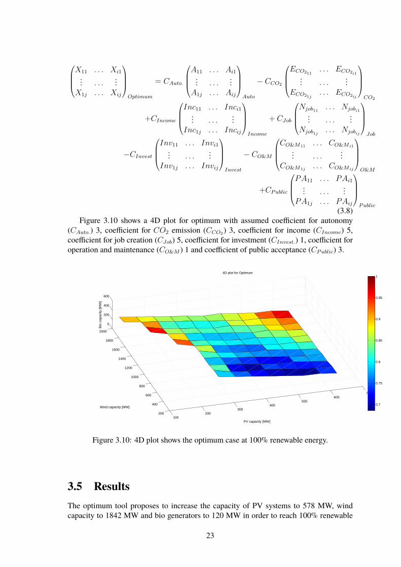
(3.8)Figure 3.10 shows a 4D plot for optimum with assumed coefficient for autonomy

(CAuto.) 3, coefficient for CO2 emission (CCO2) 3, coefficient for income (CIncome) 5,coefficient for job creation (CJob) 5, coefficient for investment (CInvest.) 1, coefficient foroperation and maintenance (CO&M ) 1 and coefficient of public acceptance (CPublic) 3.

100200

300400

500600

700

200

400

600

800

1000

1200

1400

1600

1800

2000

0

200

400

600

PV capacity [MW]

4D plot for Optimum

Wind capacity [MW]

Bio

cap

acity

[MW

]

0.7

0.75

0.8

0.85

0.9

0.95

1

Figure 3.10: 4D plot shows the optimum case at 100% renewable energy.

3.5 ResultsThe optimum tool proposes to increase the capacity of PV systems to 578 MW, windcapacity to 1842 MW and bio generators to 120 MW in order to reach 100% renewable

23

energy based on the grading scale proposed in section 3.4. That means that the regionhave to invest in 473MW in PV systems, 1535 in wind and 40MW in Bio technology.

The optimum point is sensitive many parameters such as the coefficient of gradingsystem, public acceptance, operation & maintenance, number of jobs created, investmentcosts, annual income and carbon dioxide emission for each renewable energy technology.

24

Chapter 4

Case study#1: Osnabrück, Germany

The first case study of a region, aiming to reach 100% renewable energy presented inthis master thesis is Osnabrück, Germany. Osnabrück is located in southwestern LowerSaxony on the border with Nordrhein-Westfalen. The area of the region is 2121 km2 with360,000 inhabitants. Currently the share of renewable energy in the region is around40%. The county of Osnabrück consists of 34 municipalities including 8 cities and 4 jointcommunities ranging in size from 7,000 to more than 45,000 inhabitants [16].

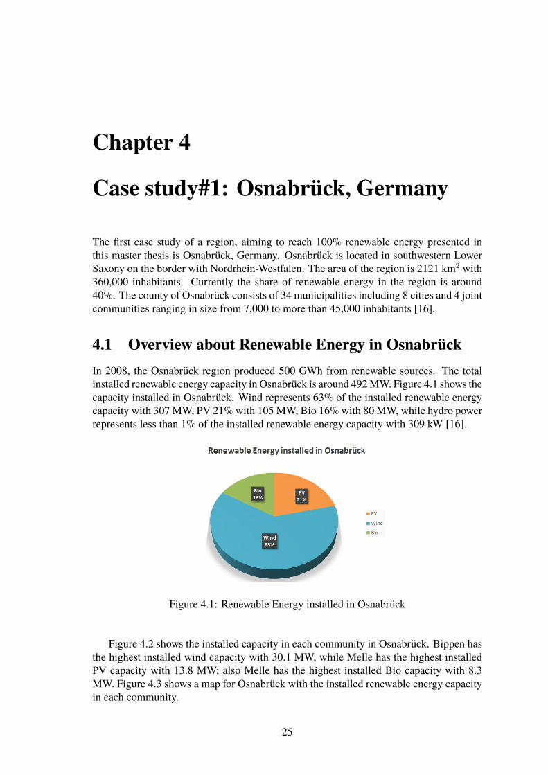
4.1 Overview about Renewable Energy in OsnabrückIn 2008, the Osnabrück region produced 500 GWh from renewable sources. The totalinstalled renewable energy capacity in Osnabrück is around 492MW. Figure 4.1 shows thecapacity installed in Osnabrück. Wind represents 63% of the installed renewable energycapacity with 307 MW, PV 21% with 105 MW, Bio 16% with 80 MW, while hydro powerrepresents less than 1% of the installed renewable energy capacity with 309 kW [16].

Figure 4.1: Renewable Energy installed in Osnabrück

Figure 4.2 shows the installed capacity in each community in Osnabrück. Bippen hasthe highest installed wind capacity with 30.1 MW, while Melle has the highest installedPV capacity with 13.8 MW; also Melle has the highest installed Bio capacity with 8.3MW. Figure 4.3 shows a map for Osnabrück with the installed renewable energy capacityin each community.

25

Figure 4.2: Installed renewable energy capacity for each community in Osnabrück

Figure 4.3: Map with Renewable energy installed in each community in Osnabrück

26

4.2 Renewable Energy Potential in Osnabrück

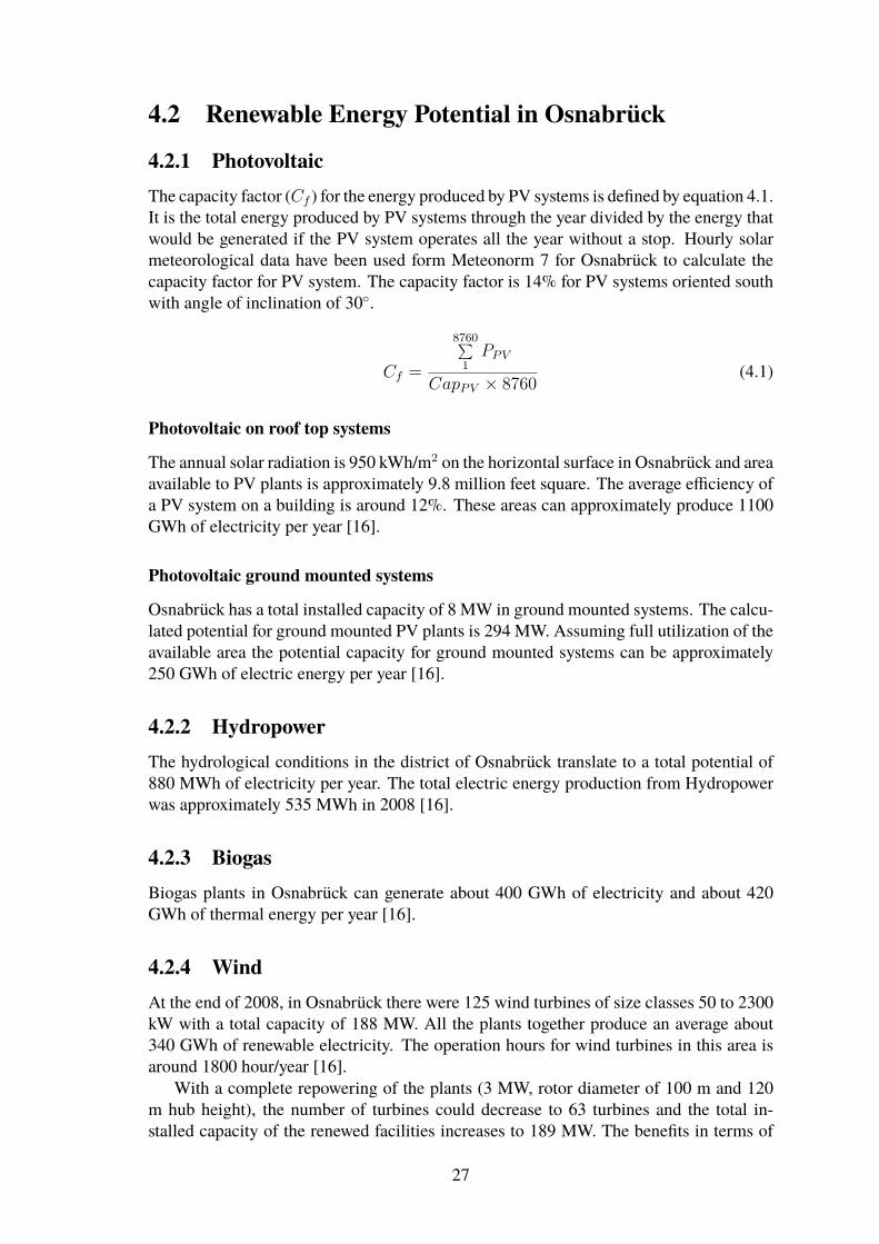
4.2.1 PhotovoltaicThe capacity factor (Cf ) for the energy produced by PV systems is defined by equation 4.1.It is the total energy produced by PV systems through the year divided by the energy thatwould be generated if the PV system operates all the year without a stop. Hourly solarmeteorological data have been used form Meteonorm 7 for Osnabrück to calculate thecapacity factor for PV system. The capacity factor is 14% for PV systems oriented southwith angle of inclination of 30◦.

Cf =

8760∑1PPV

CapPV × 8760 (4.1)

Photovoltaic on roof top systems

The annual solar radiation is 950 kWh/m2 on the horizontal surface in Osnabrück and areaavailable to PV plants is approximately 9.8 million feet square. The average efficiency ofa PV system on a building is around 12%. These areas can approximately produce 1100GWh of electricity per year [16].

Photovoltaic ground mounted systems

Osnabrück has a total installed capacity of 8 MW in ground mounted systems. The calcu-lated potential for ground mounted PV plants is 294 MW. Assuming full utilization of theavailable area the potential capacity for ground mounted systems can be approximately250 GWh of electric energy per year [16].

4.2.2 HydropowerThe hydrological conditions in the district of Osnabrück translate to a total potential of880 MWh of electricity per year. The total electric energy production from Hydropowerwas approximately 535 MWh in 2008 [16].

4.2.3 BiogasBiogas plants in Osnabrück can generate about 400 GWh of electricity and about 420GWh of thermal energy per year [16].

4.2.4 WindAt the end of 2008, in Osnabrück there were 125 wind turbines of size classes 50 to 2300kW with a total capacity of 188 MW. All the plants together produce an average about340 GWh of renewable electricity. The operation hours for wind turbines in this area isaround 1800 hour/year [16].

With a complete repowering of the plants (3 MW, rotor diameter of 100 m and 120m hub height), the number of turbines could decrease to 63 turbines and the total in-stalled capacity of the renewed facilities increases to 189 MW. The benefits in terms of

27

the achievable energy yield per plant in the same space is enormous. With each largermeter hub height the energy yield increases by approximately 1% moreover this increasesthe average permissible full load operation hours after repowering to approximately 2500hour/year [16].

4.3 Electric demand for OsnabrückIn 2008, the electric consumption for county Osnabrück was 1782 GWh. The householdconsumed 557 GWh, while the commercial and industrial sectors1 consumed 1225 GWh.The current share for the households is relatively constant in all communities at an av-erage 1425 kWh/capita. The share of the industrial and commercial sectors is subject tothe local commercial structure [16]. Figure 4.4 shows the annual expected electric en-ergy consumption and energy generated by renewable energy from 2010 until 2050 in thecounty of Osnabrück. It is expected that the energy generated from renewable sourceswould be able to fulfill the load demand in 2030, without including electric mobility andby 2050, with electric mobility.

Figure 4.4: The annual expected electric energy consumption and energy generated fromrenewable sources from 2010 until 2050 in the county of Osnabrück

1The industrial sector doesn’t include steel plants. The steel plants in the county consumes around 500GWh. [16]

28

4.4 Load profile for OsnabrückThe hourly load profile for the county of Osnabrück wasn’t provided to us, so the loadprofile has been generated for the county from the hourly load profile provided by thestadtwerke-osnabrück [17]. The load profile for 2030 for the county of Osnabrück hasbeen generated by multiplying the stadtwerke-osnabrück load profile by a factor whichis the ratio between the expected energy consumed in the county in 2030 and the energyconsumption for the region supplied by stadtwerke-osnabrück. Equation 4.2 shows howthe load profile for 2030 for the county of Osnabrück. Figure 4.5 shows hourly load profilefor the county of Osnabrück in 2030. The minimum expected load is 105 MW, while themaximum expected load is 495 MW in 2030.

PLoad1

...PLoad8760

2030(county)

=

PLoad1

...PLoad8760

2011(Stadtwerke)

×

8760∑1PLoad2030

8760∑1PLoad2011

(4.2)

0 1000 2000 3000 4000 5000 6000 7000 80000

50

100

150

200

250

300

350

400

450

500

Time [hour]

Pow

er [M

W]

Figure 4.5: The expected hourly load profile for the county Osnabrück in 2030

29

4.5 Simulation load profile with renewable energyAs has been mentioned in section 3.5 the county needs to increase the capacity of PVsystems to 578 MW, wind to 1842 MW and Bio generators to are 120 MW to reach its’goal of 100% renewable energy.

It has been assumed that 378 MW from the PV systems are from panels that south ori-ented with angle of inclination 30◦, 100 MW south east oriented with angle of inclination25◦ and the last 100 MW are south west oriented with angle of inclination 25◦.

The wind turbines needed to be installed in the county of Osnabrück have been dividedinto three categories. The first category is 82 wind turbines of ENERCON E-126 witha rated power 7.5 MW, while the second and third categories are 409 wind turbines ofENERCON E-101 and ENERCON E-82 with a rated power 3 MW.

The county of Osnabrück needs to install 40 MW of Bio generators. It has been as-sumed that this new capacity is divided between 226 Bio generators.

4.6 ResultsFigure 4.6 shows the gross, net load profile and power generated by renewable energy for48 hours. The y-axis of this graph represents the power inMW, while the x-axis representsthe time in hours. The solid black line represents the gross load profile for the county ofOsnabrück for 48 hours, while the dashed black line represents the net load profile, whichis the gross load profile subtracted from it the power generated by renewable energy in thecounty of Osnabrück. The solid orange line represents the total power produced by all PVinstalled in the county. The solid blue line represents the total power produced by all thewind turbines installed in the county. The solid green line represents the power producedby all Bio generators in the county. The net load profile is the result of subtraction of thesum of all the renewable energy technologies from the gross load profile.

Positive net loadmeans that the county imports power from outside the county to fulfillthe electric load demand, as the power produced by renewable energy technologies in thecounty is not enough to fulfill the electric load demand. Negative net load means that thecounty produces electric power higher than the electric load demand in the county andthis extra power is exported outside the county.

30

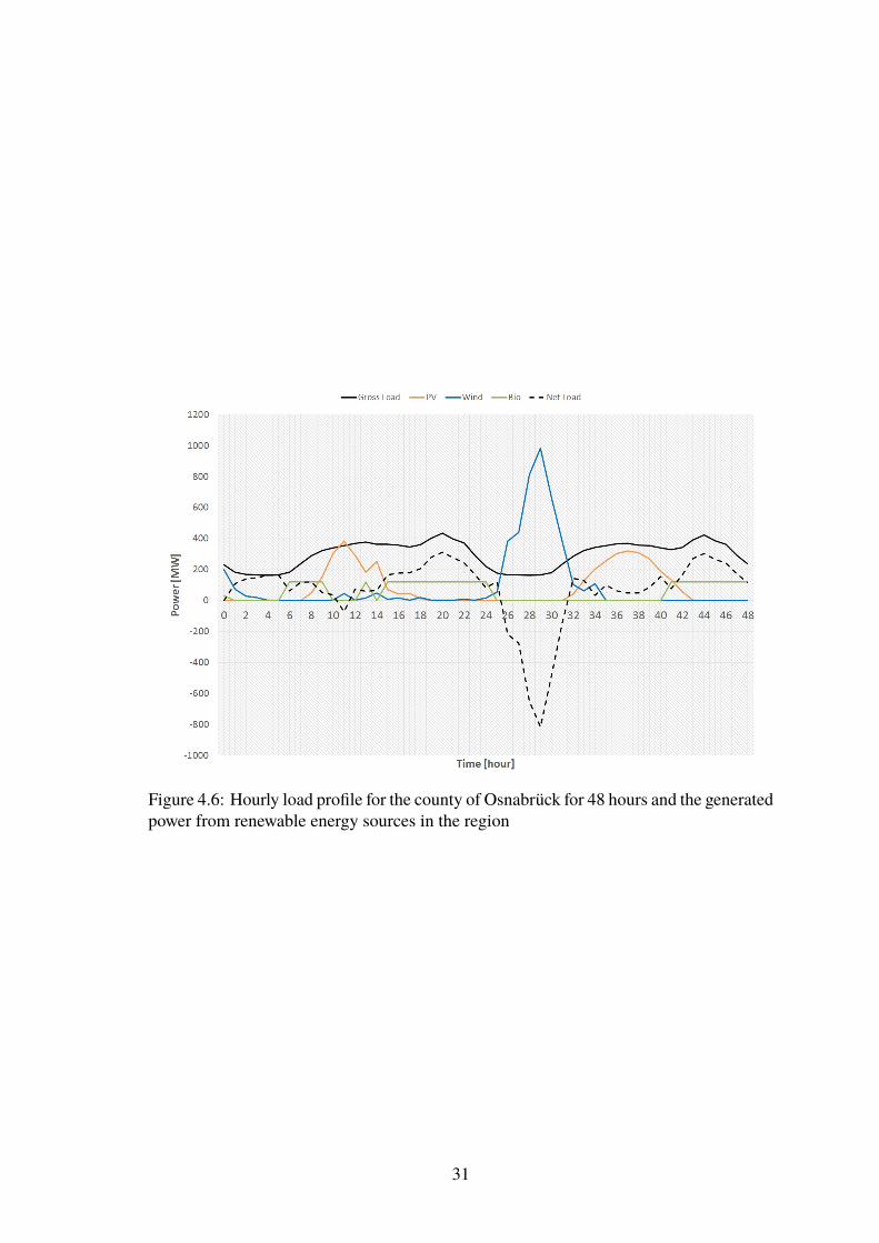
Figure 4.6: Hourly load profile for the county of Osnabrück for 48 hours and the generatedpower from renewable energy sources in the region

31

32

Chapter 5

Case study#2: Siwa, Egypt

The second case study of a region aiming to reach 100% renewable energy presentedin this master thesis is Siwa, Egypt. Siwa is located between the Qattara Depressionand the Egyptian Sand Sea, nearly 300 km south of Mersa Matruh, Egypt, 50 km eastof the Libyan border and 700 km from Cairo, Egypt. The Siwa oasis is located in adeep depression that extends below sea level. This depression, an area lower than thesurrounding region, reaches to about -19 m. Agriculture is the main activity of the Siwi,particularly the cultivation of dates and olives. Siwa consists of 11 Tribes, with around30,000 inhabitants. The information provided in this chapter about the Siwa grid, is basedon an interview with Eng. Ali Abdelnaby, head of the Siwa Engineering sector, El-Beheradistribution company from 30th of December 2012 to 2nd of January 2013.

5.1 Overview about Siwa electric grid

5.1.1 Grid historyElectricity entered Siwa during the end of 1960s. Due to increase in the electric demandthe government had to install 4 generators each of 680 kVA (2 generators were workingduring day and the other 2 during evening). The transmission network during this periodwas on 3.3 kV. Due to the start of the olive oil and water packaging industry in Siwa, theelectric demand increased and the government had to install between 1991 and 1996, 3electric generators, each generator with a capacity of 2.5 MW. Those generators operateon diesel fuel and consumed 1 liter of diesel to produce 3.2 kWh.

Until now, Siwa is not connected to the Egyptian national grid. It is 100 km awayfrom the Libyan grid and 300 km from Egyptian national grid through Mersa Matruh.Siwa is divided into 6 communities which are Siwa city, Agorny, Abo-Shrof, Al-Maraky,Baha-El-Din and Om-El-Sager. Siwa city, Agorny, Al-Marak and Baha-El-Din are con-nected with the Siwa grid. While Om-El-Sager and part of Abo-Shrof (Ayn-Zahra dis-trict) are operating on PV systems. Each house, mosque and light pole in Om-El-Sagerand Ayn-Zahra are operating as an island system, with PV modules on the roof, batteriesand inverters.

5.1.2 Electric EnergyFigure 5.1 shows the monthly electric energy consumption for Siwa for 2011 and 2012.It is noticed from figure 5.1 that there is increase in the electric demand from one year to

33

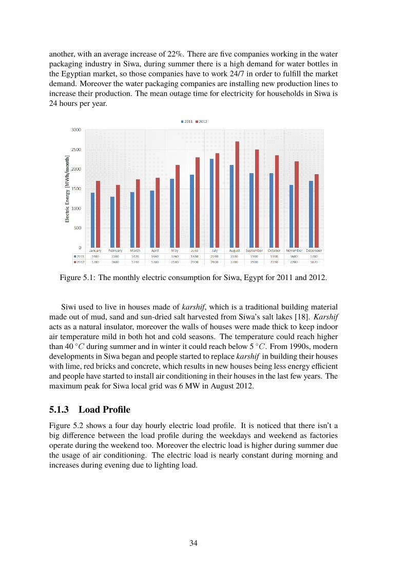
another, with an average increase of 22%. There are five companies working in the waterpackaging industry in Siwa, during summer there is a high demand for water bottles inthe Egyptian market, so those companies have to work 24/7 in order to fulfill the marketdemand. Moreover the water packaging companies are installing new production lines toincrease their production. The mean outage time for electricity for households in Siwa is24 hours per year.

Figure 5.1: The monthly electric consumption for Siwa, Egypt for 2011 and 2012.

Siwi used to live in houses made of karshif, which is a traditional building materialmade out of mud, sand and sun-dried salt harvested from Siwa’s salt lakes [18]. Karshifacts as a natural insulator, moreover the walls of houses were made thick to keep indoorair temperature mild in both hot and cold seasons. The temperature could reach higherthan 40 ◦C during summer and in winter it could reach below 5 ◦C. From 1990s, moderndevelopments in Siwa began and people started to replace karshif in building their houseswith lime, red bricks and concrete, which results in new houses being less energy efficientand people have started to install air conditioning in their houses in the last few years. Themaximum peak for Siwa local grid was 6 MW in August 2012.

5.1.3 Load ProfileFigure 5.2 shows a four day hourly electric load profile. It is noticed that there isn’t abig difference between the load profile during the weekdays and weekend as factoriesoperate during the weekend too. Moreover the electric load is higher during summer duethe usage of air conditioning. The electric load is nearly constant during morning andincreases during evening due to lighting load.

34

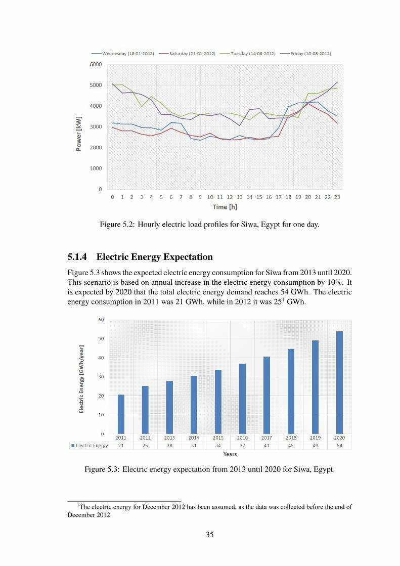
Figure 5.2: Hourly electric load profiles for Siwa, Egypt for one day.

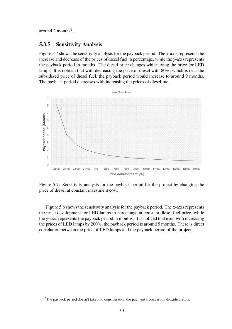
5.1.4 Electric Energy ExpectationFigure 5.3 shows the expected electric energy consumption for Siwa from 2013 until 2020.This scenario is based on annual increase in the electric energy consumption by 10%. Itis expected by 2020 that the total electric energy demand reaches 54 GWh. The electricenergy consumption in 2011 was 21 GWh, while in 2012 it was 251 GWh.

Figure 5.3: Electric energy expectation from 2013 until 2020 for Siwa, Egypt.

1The electric energy for December 2012 has been assumed, as the data was collected before the end ofDecember 2012.

35

5.2 Energy Efficiency PotentialBefore analyzing the Siwa region and how this region could reach 100% renewable energy,there should be an energy efficient auditing done to the region to reduce the electric energyconsumption, to facilitate the path to 100% renewable energy. There are 3000 street lightpoles in Siwa. The power for each street light pole is 280W, thus the total electric load forstreets light poles is 840 kW, which represents more than 10% of the electric load duringevening. Two scenarios have been proposed to reduce the electric load for street lightpoles:

1. To replace the current street light poles with new ones operating with PV moduleswith batteries as a storage. The new street light poles would be working as an islandsystem and won’t be connected with electric grid.

2. To keep the same street light poles and replace the lamps operating on 280 W withnew Light Emitting diode (LED) ones operating on 60 W, while keeping the streetlight poles connected to the grid as it is.

In both scenarios the street light poles are going anyway to operate on renewable en-ergy. The second scenario has been chosen because:

• The investment costs for the second scenario is less.

• In the first scenario the grid won’t benefit from the battery storage by the street lightpoles.

• The available light pole is quite new and reinvestment in new street light leaving thegrid connection for street light poles is considered wastage of public money.

Figure 5.4 shows the old and new winter load profile after replacing the old streetlamps by new LED lamps. It has been assumed that the street lights operate from 6 PMuntil 7 AM in January. The energy consumed by old load profile is 74 MWh, while thenew load profile consumes 64 MWh, which means that replacing the lamps could reducethe energy consumption by more than 12%.

36

Figure 5.4: Old and new electric load profile after replacing the old street lamps by newLED lamps.

5.3 Pre-Feasibility study for replacing current street lampsby LED lamps

5.3.1 IntroductionThis section is going to study from the economic point of view replacing current lampsby LED lamps. The power of the current installed street lamps is 280 W, while the powerof the new LED lamps is 60 W. The life span of the new LED lamps is 50,000 hours, witha beam angle 360 degree and 5900 lm. The input voltage range for the LED lamps is85-277 VAC.

5.3.2 Investment costsThe investment cost for 1 LED is 242 EGP that includes the purchase costs, shipping andinstallation [19]. The total investment costs to replace all the street light poles in Siwa,(which are 3000 light street pole) is 727 thousand EGP.

5.3.3 Running costsIt has been assumed that Egypt imports diesel fuel at a price 1 $/l of diesel, which isequivalent to 6.73 EGP. As it have been mentioned previously in section 5.1.1 that 1 literof diesel produces 3.2 kWh for diesel generators in Siwa. That means that the cost for 1kWh is 2.1 EGP in Siwa. Figure 5.5 compares the monthly electric energy consumed byLED lamps and old lamps, while figure 5.6 compares the monthly costs for LED lampsand old lamps.

37

Figure 5.5: Monthly energy consumed by street lighting in Siwa.

Figure 5.6: Monthly energy costs form street lighting in Siwa.

5.3.4 Savings and Payback period

The old street lighting lamps consume annually 3252 MWh, while LED street lightinglamps will consume 697 MWh. That means that just replacing the old lamps with newLED lamps saves 2555 MWh, which saves around 5 Million EGP. The payback period is

38

around 2 months2.

5.3.5 Sensitivity AnalysisFigure 5.7 shows the sensitivity analysis for the payback period. The x-axis represents theincrease and decrease of the prices of diesel fuel in percentage, while the y-axis representsthe payback period in months. The diesel price changes while fixing the price for LEDlamps. It is noticed that with decreasing the price of diesel with 80%, which is near thesubsidized price of diesel fuel, the payback period would increase to around 9 months.The payback period decreases with increasing the prices of diesel fuel.

Figure 5.7: Sensitivity analysis for the payback period for the project by changing theprice of diesel at constant investment cost.

Figure 5.8 shows the sensitivity analysis for the payback period. The x-axis representsthe price development for LED lamps in percentage at constant diesel fuel price, whilethe y-axis represents the payback period in months. It is noticed that even with increasingthe prices of LED lamps by 200%, the payback period is around 5 months. There is directcorrelation between the price of LED lamps and the payback period of the project.

2The payback period doesn’t take into consideration the payment from carbon dioxide credits.

39

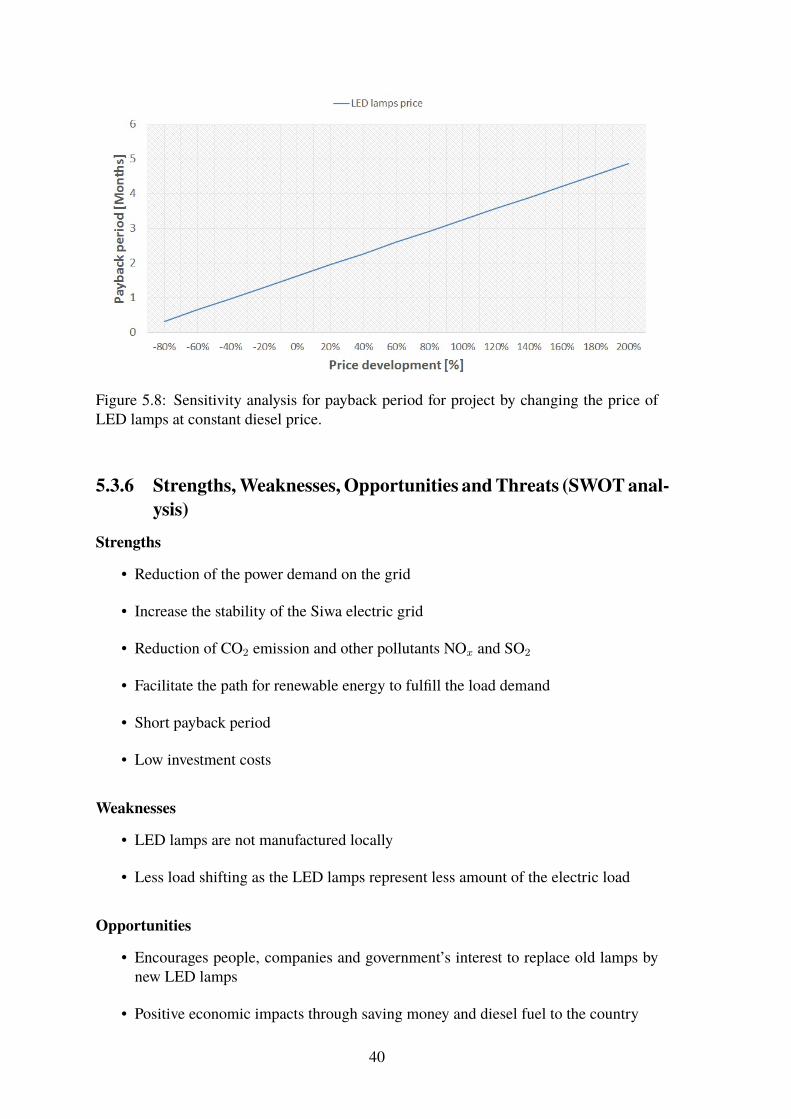
Figure 5.8: Sensitivity analysis for payback period for project by changing the price ofLED lamps at constant diesel price.

5.3.6 Strengths,Weaknesses, Opportunities andThreats (SWOTanal-ysis)

Strengths

• Reduction of the power demand on the grid

• Increase the stability of the Siwa electric grid

• Reduction of CO2 emission and other pollutants NOx and SO2

• Facilitate the path for renewable energy to fulfill the load demand

• Short payback period

• Low investment costs

Weaknesses

• LED lamps are not manufactured locally

• Less load shifting as the LED lamps represent less amount of the electric load

Opportunities

• Encourages people, companies and government’s interest to replace old lamps bynew LED lamps

• Positive economic impacts through saving money and diesel fuel to the country

40

Threats

• Awareness of energy efficiency does not reach all potentially interested parties

5.4 Potential of Renewable Energy in SiwaThis section is going to present the potential of renewable energies in Siwa. Moreover thissection is going to calculate the capacity factor for the energy produced by PV systemsand wind turbines. The capacity factor could be defined by the equation 5.1 as the totalenergy produced by a renewable energy technology through year divided by the energythat would be generated if this renewable energy technology is operating all year roundwithout stop.

Cf =

8760∑1PRE

CapRE × 8760 (5.1)

5.4.1 Wind EnergyThe average wind speed in Siwa at 10 m above the ground level is 2.4 m/sec [20]. Nordex(N43) which is installed in Zafarana, Egypt has been simulated under Siwa weather condi-tion. The capacity factor was 1.8%, which doesn’t make the region particularly interestingto install wind turbines. Figure 5.9 shows the wind atlas for Egypt, it shows that Siwa isin region class 1 [21], with low wind speeds. Moreover H. Abu ElEizz, M. Al-Motawakeland Z. Abu El-Eizz showed in their paper on "Wind characteristic and energy potential-ities of some selected sites in the Yemen Arab Republic and the Republic of Egypt" thatthe accumulated annual wind energy for Siwa is around 33 kWh/m2 and they proposedwind turbines with the following characteristics for Siwa with cut in wind speed 2 m/sec,rated wind speed 4 m/sec and cut out speed 10 m/sec [22].

Figure 5.9: Wind regime map for Egypt (Wind atlas for Egypt).

41

5.4.2 Bio EnergyThis thesis was focusing on the Bio energy generation in Siwa from garbage, animal excre-ment and wood from olive trees. Every family have a number of chickens, those chickenis feed by the remaining food from family. About the plastic garbage, all the plastic is col-lected in Siwa and recycled in Siwa and sold outside the region, so producing Bio energyfrom garbage doesn’t have high potential in Siwa. It is difficult to produce Bio energyfrom the animal excrement residues, as some families grow one or two sheeps or cowsat the backyard of the house, but there isn’t any animal farms in Siwa, so collecting theanimals excrement from large distributed area is difficult. Using wood from olive treesmeans the reduction of number of olives trees. Olives trees represents for Siwi as theirincome, so it is very hard to get red off olive tree.

5.4.3 Solar EnergySiwa has high potential for solar energy and sky is clear all over the year. Figure 5.10shows solar atlas for Egypt, the solar radiation intensity over Siwa is around 2500 kWh/m2/year[21]. The capacity factor for installed PV system in Siwa is around 29%. Moreover, it havebeen noticed that dust contamination in Siwa is very low, which reduce the need to cleanthe PV modules.

Figure 5.10: Solar radiation intensity Map for Egypt (Solar atlas for Egypt).

42

5.5 Pre-Feasibility study for 100%Renewable Energy forSiwa

5.5.1 IntroductionThis section is going to study the possibility of reaching 100% renewable energy in Siwa at2020 from the economic point of view. Figure 5.3 shows the expected energy consumptionfor Siwa region until 2020, it is expected before energy efficiency in streets light that theannual energy consumption is 54 GWh/year for 2020. On the other hand it is expected thatenergy efficiency in street lights would reduce the annual energy consumption by around2.5 GWh/year. The annual consumption after energy efficiency in street lights is around51.5 GWh/year.

5.5.2 Key Assumptions

Period of Analysis: 20 yearsTiming of Payments: At the end of each yearInterest rate: 5%Currency: EGPExchange rate: 1 $ = 6.73 EGP

1 €= 8.99 EGP

5.5.3 Renewable Energy Scenarios for SiwaAfter analyzing different renewable energy technologies in Siwa: wind energy, bio energyand solar energy, it has been notice that the best renewable energy technology for Siwa issolar energy. Siwa hasn’t been analyzed by the optimizationmethod presented in chapter 3as potential for wind energy and bio energy is very weak.

As solar energy could only supply the load only during morning, while there haveto be another solution to supply load at evening. Three scenarios have been proposed tosupply the load during all the day:

• PV system are used to supply the load during morning and charge the battery banksto supply the load during evening

• PV system are used to supply the load during morning, extra power generated by PVsystems would be exported through a transmission line to Libya and during eveningSiwa region will import power from Libya through transmission line

• PV system are used to supply the load during morning, extra power generated wouldbe exported through a transmission line to Mersa Matruh to national grid and dur-ing evening Siwa region will import power from Mersa Matruh from national gridthrough transmission line

The three scenarios would be analyzed from the investment cost point of view and theone which have the least investment cost would be further analyzed. Siwa region needs toinstall 21 MW PV systems, in order to generate annual energy 53 GWh, which is higherthan the electric energy demand by 2020 in case it is connected to Libya grid or national

43

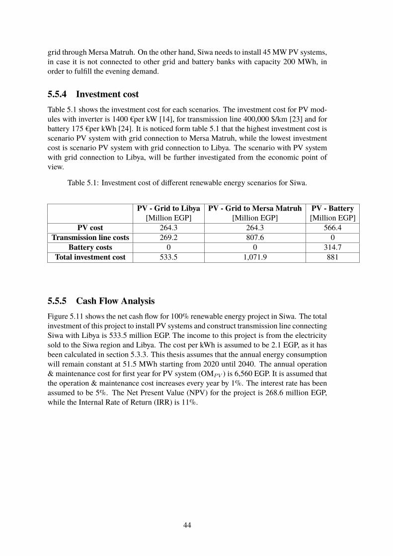
grid through Mersa Matruh. On the other hand, Siwa needs to install 45 MW PV systems,in case it is not connected to other grid and battery banks with capacity 200 MWh, inorder to fulfill the evening demand.

5.5.4 Investment costTable 5.1 shows the investment cost for each scenarios. The investment cost for PV mod-ules with inverter is 1400 €per kW [14], for transmission line 400,000 $/km [23] and forbattery 175 €per kWh [24]. It is noticed form table 5.1 that the highest investment cost isscenario PV system with grid connection to Mersa Matruh, while the lowest investmentcost is scenario PV system with grid connection to Libya. The scenario with PV systemwith grid connection to Libya, will be further investigated from the economic point ofview.

Table 5.1: Investment cost of different renewable energy scenarios for Siwa.

PV - Grid to Libya PV - Grid to Mersa Matruh PV - Battery[Million EGP] [Million EGP] [Million EGP]

PV cost 264.3 264.3 566.4Transmission line costs 269.2 807.6 0

Battery costs 0 0 314.7Total investment cost 533.5 1,071.9 881

5.5.5 Cash Flow AnalysisFigure 5.11 shows the net cash flow for 100% renewable energy project in Siwa. The totalinvestment of this project to install PV systems and construct transmission line connectingSiwa with Libya is 533.5 million EGP. The income to this project is from the electricitysold to the Siwa region and Libya. The cost per kWh is assumed to be 2.1 EGP, as it hasbeen calculated in section 5.3.3. This thesis assumes that the annual energy consumptionwill remain constant at 51.5 MWh starting from 2020 until 2040. The annual operation& maintenance cost for first year for PV system (OMPV ) is 6,560 EGP. It is assumed thatthe operation & maintenance cost increases every year by 1%. The interest rate has beenassumed to be 5%. The Net Present Value (NPV) for the project is 268.6 million EGP,while the Internal Rate of Return (IRR) is 11%.

44

Figure 5.11: The net cash flow for 100% renewable energy project in Siwa.

5.5.6 Savings and Payback Period

Figure 5.12 shows cumulative net cash flow for 100% renewable energy project in Siwa. Itis noticed from figure 5.12 that the payback period for the project is 9 years. This projectwould save around annually around 16 million liter of diesel.

Figure 5.12: The cumulative net cash for 100% renewable energy project in Siwa.

45

5.5.7 Sensitivity AnalysisIt is noted that the dominating factors in the investment cost are the investment in PV sys-tem and the transmission line connecting Libya grid with Siwa. This section will presentthe effect of changing the prices of the PV system, transmission line and interest rate onNPV and IRR. Figure 5.13 shows the the effect of the price development of PV system onthe NPV of the project, while the price for transmission lines and interest rate are constant.The x-axis represents the development price in percentage for the PV system, while they-axis represents NPV. NPV decreases with increasing the price of the PV system. NPVstarts to be negative when the PV system cost increases by more than 40%.

Figure 5.13: Effect of price development for PV system on NPV, at constant transmissionlines cost and constant interest rate.

Figure 5.14 shows the effect of the price development of the transmission lines on theNPV of the project, while the price of the PV systems and interest rate are constant. Thex-axis represents the development price in percentage for the transmission line, while they-axis represents NPV. NPV decreases with increasing the price of transmission lines.NPV becomes negative when the price of transmission lines increases by more than 40%.

46

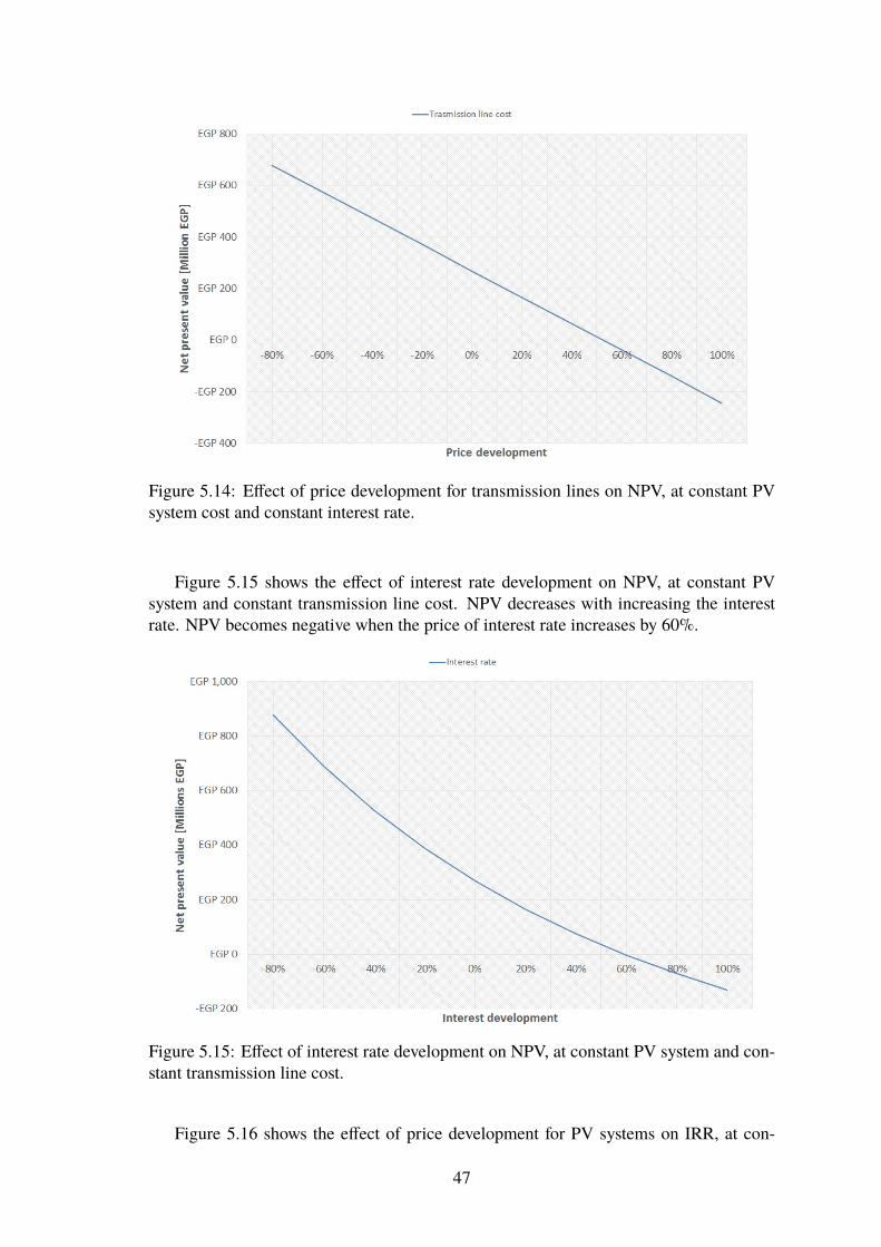
Figure 5.14: Effect of price development for transmission lines on NPV, at constant PVsystem cost and constant interest rate.

Figure 5.15 shows the effect of interest rate development on NPV, at constant PVsystem and constant transmission line cost. NPV decreases with increasing the interestrate. NPV becomes negative when the price of interest rate increases by 60%.

Figure 5.15: Effect of interest rate development on NPV, at constant PV system and con-stant transmission line cost.

Figure 5.16 shows the effect of price development for PV systems on IRR, at con-

47

stant transmission lines cost and constant interest rate. The x-axis represents the pricedevelopment in percentage for the PV system costs, while the y-axis represents IRR. IRRdecreases with increasing the PV system costs. IRR becomes less than the interest ratewhen the price of PV system costs increases by more than 40%.

Figure 5.16: Effect of price development for PV systems on IRR, at constant transmissionlines cost and constant interest rate.

Figure 5.17 shows the effect of price development for transmission lines on IRR, atconstant PV system and constant interest rate. The x-axis represents the price developmentin percentage for the transmission lines, while the y-axis represents IRR. IRR decreaseswith increasing the transmission lines costs. IRR becomes less than the interest rate whenthe price of PV system costs increases by more than 40%.

48

Figure 5.17: Effect of price development for transmission lines on IRR, at constant PVsystem cost and constant interest rate.

Figure 5.18 shows the effect of development of interest rate on IRR, at constant PVsystem and transmission line cost. The x-axis represents the effect of development ofinterest rate in percentage, at constant PV system and transmission line cost, while y-axisrepresents IRR in percentage.

Figure 5.18: Effect of interest rate development on IRR, at constant PV system and trans-mission lines cost.

49

5.5.8 Strengths,Weaknesses, Opportunities andThreats (SWOTanal-ysis)

Strengths

• Siwa grid would be operating at 100% renewable energy

• Increase the stability of the Siwa electric grid

• Increase the trade between Egypt and Libya

• Save annually 16 million liter of diesel to the country

Weaknesses

• High investment costs

• Long payback period for the project

• Increase of the prices of the investment costs or interest rate could lead that theproject is invisible

• Siwa may face black out in case of problem with transmission lines

Opportunities

• Encourages people, companies and government’s interest to start 100% renewableenergy projects in other oasis

• Positive economic impacts through saving money and diesel fuel to the country

Threats

• Siwa region would be affected by any problem happens to Libyan grid.

5.6 Simulation

5.6.1 Monthly Energy Profile 2020This master thesis is going to simulate the Siwa region at 2020 operating at 100% renew-able energy. It is assumed that the monthly consumption in 2020 is with the same ratio as2012. Figure 5.19 shows the monthly electric energy profile for Siwa in 2020. The max-imum load expected in 2020 is 9.6 MW, while the minimum load expected is 4.2 MW.

50

Figure 5.19: The expected monthly electric energy profile for Siwa in 2020.

5.6.2 Simulation load profile with renewable energySiwa region needs to install 21 MW PV system, in order to reach 100% renewable energy.There is around 30,000 inhabitant, if it is assumed that each family house have 6 persons,that means there is around 5000 house in Siwa. It have been assumed that each housewould install PV system with capacity 2.1 kWp. That means that the total installed capac-ity on the roof of the houses in Siwa is around 10.5 MWp. There are around 16 factory inSiwa, so if each factory could install between 20 and 100 kWp, so that the total installedcapacity on the roof of factories in Siwa is 750 kWp. There would be four PV power plantseach power plant is with capacity 2.5 MWp. The total PV capacity installed in Siwa is21.25 MWp. All PV system installed in Siwa is facing south with angle of inclination 30◦.This PV capacity would generate annually 54.3 GWh. The hourly meteorological data forSiwa for 2020, have been predicted by Meteonorm version 7.

The gross load profile (PLGross) is defined as the hourly electric load profile for the

region, while the net load profile (PLNet) could be defined as the gross load profile sub-

tracted from it the power generated by renewable energy within the region. Each monthin 2020 have been weighted the same ratio as the weight for 2012. The gross load profileis generated from the new day hourly load profile after applying energy efficiency to thestreet lighting in Siwa. There is two daily load profiles one for summer and the second onefor winter. The summer load profile have been applied for gross load profiles for April,May, June, July, August and September, while the winter load profile have been appliedfor gross load profiles January, February, March, October, November and December.

5.6.3 ResultsHourly net profile have been calculated by the method presented in subsection 5.6.2. Theimported and exported electric energy have been calculated and presented in figure 5.20.

51

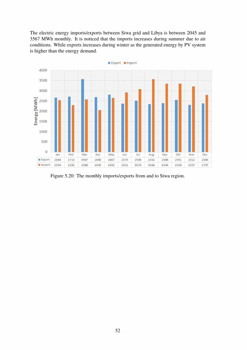
The electric energy imports/exports between Siwa grid and Libya is between 2045 and3567 MWh monthly. It is noticed that the imports increases during summer due to airconditions. While exports increases during winter as the generated energy by PV systemis higher than the energy demand.

Figure 5.20: The monthly imports/exports from and to Siwa region.

52

Chapter 6

Conclusion, Recommendations andFuture Work

6.1 ConclusionPV, wind, bio generator models have been presented in chapter 2. Those models havebeen used to represent renewable energy generators in the region. Chapter 3 presenteda new methodology to get the optimum capacity needed to be installed in order to reach100% renewable energy with in the region. This optimization tool was implemented usingMATLAB platform. The optimization tool takes into consideration autonomy, costs, CO2emission, job creation, operation & maintenance costs and public acceptance.

The county of Osnabrück could reach to 100% renewable energy by increasing theinstalled capacity of PV systems to 578MW, wind to 1842MW and Bio generators to 120MW. Hourly simulation have been presented with the new renewable energy capacities inchapter 4.

Applying energy efficiency in street lighting systems would save annually 6 millionEGP. Siwa region could reach to 100% renewable energy, by installing 21MWPV systemsand build transmission lines connecting Siwa region with Libya grid. Payback periodexpected for 100% renewable energy project in Siwa is 9 years.

6.2 RecommendationsIn chapter 3, the coefficients for the optimization method have been assumed, it is recom-mended in the future that those coefficients are done by survey for the people living in thecounty and decision makers.

Tracking PV system is much more recommended for the four PV power plants thatwould be installed in Siwa, as it would produce much more energy, moreover the powerproduced by the tracking system is over longer period of day, which reduces exportingenergy from Libya.

It is recommended to apply energy efficiency in houses in Siwa, as new houses builtwith bad energy efficiency in building, need to install air conditions, which consumes alot of energy, so applying energy efficiency into houses would reduce the load demandduring summer.

There is more than hot springs in Siwa oasis, so it is recommended to study the po-tential of producing electric energy from geothermal energy in Siwa.

53

PV systems in Om-El-Sager and Abo-Shrof regions, are operating as island systemfor each house. That means that each house have his own modules, battery and inverter.The problem with this system that new houses built won’t have electricity and on the otherhand people living there could afford to buy this PV system. So it is recommended in thefuture to make an internal grid for the region and make central battery bank, so that newhouses built could have electricity.

This master focus on reaching with region to 100% renewable energy, which requiresfrom Siwa region to build transmission lines or install battery bank, which increases theinvestment costs. On the other hand Siwa region could start to install PV systems to supplythemorning demand, while during night it could operate the diesel generators to supply thenight demand. Although this scenario won’t reach with Siwa region to 100% renewableenergy, it would reduce the CO2 emission for the region and diesel consumption.

6.3 Future WorkThe algorithm for optimization tool needs to be further improved to reduce the computa-tion time. Moreover the optimization tool needs to add a new optimization tool, such asthe number of bio generators that needed to be installed.

The simulation tool for renewable energy needs to be modified to present the gridproblems and what needed to be changed in the infrastructure of the grid to be operatingat 100% renewable energy.

54

Bibliography

[1] H. Lund, Renewable Energy Systems: The Choice andModeling of 100%RenewableSolutions. Elsevier Science, 2009.

[2] H. Lund, “Renewable energy strategies for sustainable development,” Energy,vol. 32, no. 6, pp. 912 – 919, 2007. Third Dubrovnik Conference on SustainableDevelopment of Energy, Water and Environment Systems.

[3] D. Connolly, H. Lund, B. Mathiesen, and M. Leahy, “The first step towards a 100%renewable energy-system for ireland,” Applied Energy, vol. 88, no. 2, pp. 502 – 507,2011. The 5th Dubrovnik Conference on Sustainable Development of Energy, Waterand Environment Systems, held in Dubrovnik September/October 2009.

[4] M. Kruska, D. Ichiro, M. Ohbayash, K. Takase, I. Tetsunari, G. Evans, S. Herbergs,H. Lehmann, K. Mallon, S. Peter, and D. Assman, “Energy rich japan,” tech. rep.,EUTech, Institute for Sustainable Energy Policies (ISEP), Institute for SustainableSolutions and Innovations (ISUSI), Wuppertal Institute for Climate, Environmentand Energy, Römerweg 2, 52070 Aachen, Germany, October 2003.

[5] B. V. Mathiesen, H. Lund, and K. Karlsson, “100% renewable energy systems, cli-mate mitigation and economic growth,” Applied Energy, vol. 88, no. 2, pp. 488 –501, 2011. The 5th Dubrovnik Conference on Sustainable Development of Energy,Water and Environment Systems, held in Dubrovnik September-October 2009.

[6] A. Wagner, Photovoltaik Engineering.: Die Methode der Effektiven Solarzellen-Kennlinie. VDI-Buch, Springer-Verlag GmbH, 1999.

[7] C. Bendel and A. Wagner, “Photovoltaic measurement relevant to the energy yield,”in Photovoltaic Energy Conversion, 2003. Proceedings of 3rd World Conference on,vol. 3, pp. 2227 –2230 Vol.3, may 2003.

[8] H. Schmidt and D. U. Sauer, “Praxisgerechte modellierung und abschaetzung vonwechselrichter-wirkungsgraden,” Sonnenenergie, no. 4, pp. 43–47, 1996.

[9] M. Ammon, “Grid parity of photovoltaics in germany a result of the renewable en-ergy act,” IMRE, vol. 6, no. 1, pp. 15–27, 2012.

[10] M. Ray, A. Rogers, and J. McGowan, “Analysis of wind shear models and trends indifferent terrains,” in AWEA Windpower 2005 Conference, June 2006.

[11] S. Muyeen, J. Tamura, and T. Murata, Stability Augmentation of a Grid-ConnectedWind Farm. Green energy and technology, Springer, 2009.

55

[12] H. Lund and B. Mathiesen, “Energy system analysis of 100systems - the case ofdenmark in years 2030 and 2050,” Energy, vol. 34, no. 5, pp. 524 – 531, 2009. 4thDubrovnik Conference 4th Dubrovnik conference on Sustainable Development ofenergy, Water and amp; Environment.

[13] J. Sievers, Dieselmotor-Kraft-Wärme-Kopplungsanlagen im Kontext der Integrationerneuerbarer Energien in die Energieversorgung. PhD thesis, Universität Kassel,2010.

[14] “Renewable power generation: Costs in 2012: An overview,” tech. rep., Interna-tional Renewable Energy Agency (IRENA), C67 Office Building, Khalidiyah (32nd)Street, 236, Abu Dhabi, United Arab Emirates, January 2013.

[15] “Renewable energy jobs & access,” tech. rep., International Renewable EnergyAgency (IRENA), C67 Office Building, Khalidiyah (32nd) Street, 236, Abu Dhabi,United Arab Emirates, June 2012.

[16] A. Witte, I. Lehmkuhl, D. Vagelpohl, A. Graw, K. Reisdorf, D. Genske, A. Ruff,T. Jödecke, P. Moser, and C. H. and, “Integriertes klimaschutzkonzept des landkreisosnabrück,” tech. rep., Landkreis Osnabrück, Planungsbüro Graw and Kompeten-znetzwerk Dezentrale Energietechnologien GmbH, Universität Kassel, FachgebietÖkonomie der Stadt- und Regionalentwicklung, 2011.

[17] D. S. der Stadtwerke Osnabrück AG, “Netzstrukturstrukturdaten,” 2012.

[18] C. Brebbia, Eco-Architecture: Harmonisation Between Architecture and Nature.WIT Transactions on Ecology and the Environment, WIT Press, 2012.

[19] “Shenzhen snc opto electronic company, led street light,” 2013.

[20] K. S. Essa and F. Mubarak, “Survey and assessment of wind-speed and windpowerin egypt, including air density variation,” Wind Engineering, vol. 30, no. 2, pp. 95–106, 2006.

[21] A. K. Khalil, A. M. Mubarak, and S. A. Kaseb, “Road map for renewable energyresearch and development in egypt,” Journal of Advanced Research, vol. 1, no. 1,pp. 29 – 38, 2010.

[22] H. A. El-Eizz, M. Al-Motawakel, and Z. A. El-Eizz, “Wind characteristic and energypotentialities of some selected sites in the yemen arab republic and the republic ofegypt,” Renewable Energy, vol. 1, no. 5–6, pp. 675 – 681, 1991.

[23] “100 per cent renewables study – electricity transmission cost assumptions,” tech.rep., Australian Energy Market Operator (AEMO), September 2012.

[24] “Photon magazine, august 2011.”

56