Embed Size (px)
Citation preview
Proceedings, 6th Chaotic Modeling and Simulation International Conference
11 - 14 June 2013 Istanbul, Turkey
Simulation of a Network Circulars Patch Antennas
for the Wireless Communications
Adnane Latif
Cadi Ayyad University, Marrakech, Morocco
E-mail: [email protected], [email protected]
Abstract:
The objective of this paper is the design a linear network of 3 circular patch antennas
and the study its radiation diagrams which is formed by multiplying a diagram of a
single patch antenna by the factor of a linear network in the two planes E and H .In fact
, the change excitation phase β which is considered as very important parameter in the
patch antenna network design is adjusted while all the other factors are fixed, thus, the
different radiation diagrams of the network in two planes are obtained .
Keywords: Patch antenna, Array antennas, Wireless communications, Radiation
Diagramm, Simulation of antenna network.
1. Introduction The use of a single patch antenna is often insufficient to meet the constraints
imposed by radiation. Specific characteristics such as high gain or a main lobe
comply can usually be obtained only by grouping several sources radiating to
form a system called "network". A network of antennas consists of a group of
identical sources. The spacing of the sources called “network step” which is a
basic parameter in the design of a network patch antenna.
These sources are fed by a splitter (distribution system) which defines a law of
supply in module and in phase. The major advantage of the network of antennas
is the ability to create a radiation beam adjustable and shaped in all directions
according to the law of supply and the number of elements. The group in the
simplest network is obtained with a number of identical sources that are
deduced from each other by translation to form linear networks and plans.
For the linear network, we seek to conform the radiation diagram only in the
plane containing the sources. In a modification of the radiation diagram over the
entire hemisphere, the elementary sources must be arranged in the two-
dimensional network.
In an antennas network, the energy is distributed between various sources
radiating in a given law: the radiation characteristics of the system depends on
the radiation diagram of the base element, the coefficients of excitation in
amplitude and in phase on each source and the distance between elements.
These networks consist of circular radiating elements connected in chain with
each other by short cut of microstrip line. The supply network of the antenna
will aim to bring energy to the various sources according to the law of
weighting (balance). The simplest technique is to feed the radiating elements by
microstrip lines.
325

Proceedings, 6th Chaotic Modeling and Simulation International Conference
11 - 14 June 2013 Istanbul, Turkey
2. Radiation Diagram of a Network of Circular Patch Antenna
A linear network with uniform spacing is illustrated in Figure 1.1 where N
isotropic radiating elements are excited by a plane wave generated from source
situated in a far field. The field radiated by an antenna network is the vector
summation of fields radiated by each element. By properly selecting the spacing
between the elements and power law, we can change the directivity and the
radiation direction of the network.
Figure 1 .Network of N circular patch aligned along the z axis
θ: The angle between the z axis is the direction of radiation
φ: The angle between the projection of the direction of radiation and x-axis
β: The phase of current between two successive elements in the network
3. Simulation of a Linear Network Formed by Three Circular
Patch Antennas The simulation of linear network will be made on two softwares MATLAB and
PCAAD. The used parameters of this antenna are:
The ray of the patch a =3cm
The dielectric constant ɛr =2.33
The thickness dielectric h=0.159cm
Frequency of resonance fr =2.3 GHz
Length of wave λ =3cm
For this network the number of patches is N = 3 is the spacing between the
elements is fixed at 7cm.
The results of the program developed in MATLAB are mounted in the figures 2
and 3, in which visualizes the network factor of the 3 antennas patch polar
coordinates and Cartesian coordinates, and the radiation diagram of a single
circular patch antenna and the radiation diagram of the network of 3 circular
patch antennas.
326

Proceedings, 6th Chaotic Modeling and Simulation International Conference
11 - 14 June 2013 Istanbul, Turkey
3.1 In the E Plane(φ=0)
For different values of phase network , it visualizes the diagram of radiation
observed in the network plan E. The result is shown on the figures below:
0.5
1
30
210
60
240
90
270
120
300
150
330
180 0
Facteur de Reseau en coordonnées polaire
25
50
30
210
60
240
90
270
120
300
150
330
180 0
Diagramme de Rayonnement de patch isolé
25
50
30
210
60
240
90
270
120
300
150
330
180 0
Diagramme de Rayonnement de Reseau de patch
-100 -50 0 50 1000
0.5
1Facteur de Reseau en coordonnées cartesiennes
360,0
0.5
1
30
210
60
240
90
270
120
300
150
330
180 0
Facteur de Reseau en coordonnées polaire
25
50
30
210
60
240
90
270
120
300
150
330
180 0
Diagramme de Rayonnement de patch isolé
25
50
30
210
60
240
90
270
120
300
150
330
180 0
Diagramme de Rayonnement de Reseau de patch
-100 -50 0 50 1000
0.5
1Facteur de Reseau en coordonnées cartesiennes
45
327

Proceedings, 6th Chaotic Modeling and Simulation International Conference
11 - 14 June 2013 Istanbul, Turkey
0.5
1
30
210
60
240
90
270
120
300
150
330
180 0
Facteur de Reseau en coordonnées polaire
25
50
30
210
60
240
90
270
120
300
150
330
180 0
Diagramme de Rayonnement de patch isolé
25
50
30
210
60
240
90
270
120
300
150
330
180 0
Diagramme de Rayonnement de Reseau de patch
-100 -50 0 50 1000
0.5
1Facteur de Reseau en coordonnées cartesiennes
90
0.5
1
30
210
60
240
90
270
120
300
150
330
180 0
Facteur de Reseau en coordonnées polaire
25
50
30
210
60
240
90
270
120
300
150
330
180 0
Diagramme de Rayonnement de patch isolé
25
50
30
210
60
240
90
270
120
300
150
330
180 0
Diagramme de Rayonnement de Reseau de patch
-100 -50 0 50 1000
0.5
1Facteur de Reseau en coordonnées cartesiennes
130
328

Proceedings, 6th Chaotic Modeling and Simulation International Conference
11 - 14 June 2013 Istanbul, Turkey
0.5
1
30
210
60
240
90
270
120
300
150
330
180 0
Facteur de Reseau en coordonnées polaire
25
50
30
210
60
240
90
270
120
300
150
330
180 0
Diagramme de Rayonnement de patch isolé
25
50
30
210
60
240
90
270
120
300
150
330
180 0
Diagramme de Rayonnement de Reseau de patch
-100 -50 0 50 1000
0.5
1Facteur de Reseau en coordonnées cartesiennes
300
0.5
1
30
210
60
240
90
270
120
300
150
330
180 0
Facteur de Reseau en coordonnées polaire
25
50
30
210
60
240
90
270
120
300
150
330
180 0
Diagramme de Rayonnement de patch isolé
25
50
30
210
60
240
90
270
120
300
150
330
180 0
Diagramme de Rayonnement de Reseau de patch
-100 -50 0 50 1000
0.5
1Facteur de Reseau en coordonnées cartesiennes
345
Figure 2. Diagram of radiation linear network with N = 3 in the E plane
(MATLAB)
For the results we have found for the same values of phase network using the
software PCAAD are shown below Fig.3:
329
Proceedings, 6th Chaotic Modeling and Simulation International Conference
11 - 14 June 2013 Istanbul, Turkey
360,0 45
90 130
300 ° 345
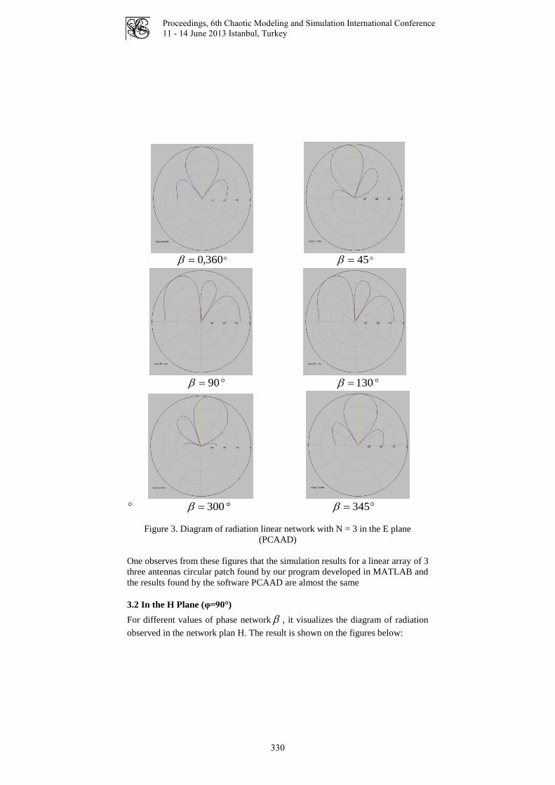
Figure 3. Diagram of radiation linear network with N = 3 in the E plane
(PCAAD)
One observes from these figures that the simulation results for a linear array of 3
three antennas circular patch found by our program developed in MATLAB and
the results found by the software PCAAD are almost the same
3.2 In the H Plane (φ=90°)
For different values of phase network , it visualizes the diagram of radiation
observed in the network plan H. The result is shown on the figures below:
330

Proceedings, 6th Chaotic Modeling and Simulation International Conference
11 - 14 June 2013 Istanbul, Turkey
1
2
30
210
60
240
90
270
120
300
150
330
180 0
Facteur de Reseau en coordonnées polaire
25
50
30
210
60
240
90
270
120
300
150
330
180 0
Diagramme de Rayonnement de patch isolé
50
100
30
210
60
240
90
270
120
300
150
330
180 0
Diagramme de Rayonnement de Reseau de patch
-100 -50 0 50 1001.7
1.8
1.9
2Facteur de Reseau en coordonnées cartesiennes
360,0
1
2
30
210
60
240
90
270
120
300
150
330
180 0
Facteur de Reseau en coordonnées polaire
25
50
30
210
60
240
90
270
120
300
150
330
180 0
Diagramme de Rayonnement de patch isolé
50
100
30
210
60
240
90
270
120
300
150
330
180 0
Diagramme de Rayonnement de Reseau de patch
-100 -50 0 50 1001.4
1.6
1.8
2Facteur de Reseau en coordonnées cartesiennes
45
331

Proceedings, 6th Chaotic Modeling and Simulation International Conference
11 - 14 June 2013 Istanbul, Turkey
1
2
30
210
60
240
90
270
120
300
150
330
180 0
Facteur de Reseau en coordonnées polaire
25
50
30
210
60
240
90
270
120
300
150
330
180 0
Diagramme de Rayonnement de patch isolé
50
100
30
210
60
240
90
270
120
300
150
330
180 0
Diagramme de Rayonnement de Reseau de patch
-100 -50 0 50 1001.4
1.6
1.8
2Facteur de Reseau en coordonnées cartesiennes
90
1
2
30
210
60
240
90
270
120
300
150
330
180 0
Facteur de Reseau en coordonnées polaire
25
50
30
210
60
240
90
270
120
300
150
330
180 0
Diagramme de Rayonnement de patch isolé
50
100
30
210
60
240
90
270
120
300
150
330
180 0
Diagramme de Rayonnement de Reseau de patch
-100 -50 0 50 1001.4
1.6
1.8
2Facteur de Reseau en coordonnées cartesiennes
130
332

Proceedings, 6th Chaotic Modeling and Simulation International Conference
11 - 14 June 2013 Istanbul, Turkey
1
2
30
210
60
240
90
270
120
300
150
330
180 0
Facteur de Reseau en coordonnées polaire
25
50
30
210
60
240
90
270
120
300
150
330
180 0
Diagramme de Rayonnement de patch isolé
50
100
30
210
60
240
90
270
120
300
150
330
180 0
Diagramme de Rayonnement de Reseau de patch
-100 -50 0 50 1001.4
1.6
1.8
2Facteur de Reseau en coordonnées cartesiennes
300
1
2
30
210
60
240
90
270
120
300
150
330
180 0
Facteur de Reseau en coordonnées polaire
25
50
30
210
60
240
90
270
120
300
150
330
180 0
Diagramme de Rayonnement de patch isolé
50
100
30
210
60
240
90
270
120
300
150
330
180 0
Diagramme de Rayonnement de Reseau de patch
-100 -50 0 50 1001.6
1.7
1.8
1.9
2Facteur de Reseau en coordonnées cartesiennes
345
Figure 4. Diagram of radiation linear network with N = 3 in the E plane
(MATLAB)
333

Proceedings, 6th Chaotic Modeling and Simulation International Conference
11 - 14 June 2013 Istanbul, Turkey
For the results we have found for the same values of phase network using
the software PCAAD are shown below Figure 5:
360,0 45
90 130
300 345
Figure 5. Diagram of radiation linear network with N = 3 in the H plane
(PCAAD)
The simulation results for the linear network of 3 circular patch antennas in H
plan our program developed in MATLAB and the results found by the PCAAD
software are almost the same.
334

Proceedings, 6th Chaotic Modeling and Simulation International Conference
11 - 14 June 2013 Istanbul, Turkey
4. Conclusions In E plane: According to the result given by the software PCAAD and those
found by MATLAB: We observe that the phase variation of excitation
influences only on the directivity pattern. a good directivity of the radiation
diagram is observed for 0 (12.0 dB). We observe also an increase in
modulus of the deflection angle is obtained by varying the phase excitation from 00 (where the deflection angle equal to
00 ) to 0130 (or
deviation angle equal to 033 ) after it decreases from
0300 (where
deflection angle equal to015 ). On the main lobe amplitude is reduced by
increasing the phase excitation from00 to
0130 at the same time the
amplitude of side lobes increases, but the main lobe amplitude starts has
increased from0300 .
In H plane: According to the result given by the software MATLAB and
PCAAD: It is observed that an increase in excitation phase has an effect only on
the directivity of the network diagram, on the other hand the width of 3dB beam
remains constant during this phase variation of excitation (76.7 °) as well as
deflection angle of main lobe is always zero (0 °). In order the directivity
remains constant for the value = 0 °, 45 ° (its value equal to 12dB), begins to
decline after increasing the excitation phase ( = 90 ° for the value of
directivity is 11.8dB, for = 130 No value of directivity is 11.1dB), after
beginning to increase for = 300 ° (11.9dB), and = 345 (12dB).
References 1. D.M. Pozar and D.H.Schaubert, New York, IEEE Press, 1995.
2. K.Huie, Thesis submitted to the faculty of the Virginia Polytechnic Institute and
State University in partial fulfilment of the requirements for the degree of Master
of Science in Electrical Engineering, January, 2002
3. C.A. Balanis, 2nd
Edition, John Wiley & Son, Inc 1997.
4. F.T. Ulaby, Prentice Hall, 1999.
5. A. Constantine - Balanis, 3ième Edition John Wiley & Sons Inc 2005.
6. W.F. Richards, Van Nostrand Reinhold Co.,New York , 1989.
7. J.R. James and P.S. Hall, I.E.E. Electromagnetic Waves Series 28, Peter Peregrinus
LTD 1989
8. Constantine A. Balanis , John Wiley & Son,Inc, 2008.
9. E.H Newman,and P.Tylythan, 1981.
10. R.F. Harrington, New York, 1968.
335

Proceedings, 6th Chaotic Modeling and Simulation International Conference
11 - 14 June 2013 Istanbul, Turkey
336

Proceedings, 6th Chaotic Modeling and Simulation International Conference
11 - 14 June 2013 Istanbul, Turkey
Resonances and patterns within the kINPen-MED
atmospheric pressure plasma jet
Victor J Law, A Chebbi, F T O’Neill and D P Dowling
School of Mechanical and Materials Engineering, University College Dublin,
Belfield, Dublin 4, Ireland.
E-mail: [email protected]
Abstract: The kINPen MED atmospheric pressure plasma jet is now undergoing clinical
studies that are designed to investigate its suitability as a device for use in plasma
medicine treatments. This paper describes dimensionless studies of the synchronizing
oscillatory gas flow through the nozzle followed by electro-acoustic measurements
coupled with the discharge photo emission. The plasma jet operates in the burst mode of
2.5 KHz (duty cycle = 50%), within a neutral argon Strouhal number of 0.14 to 0.09 and
Reynolds number of 3570 to 5370. In this mode the jet acts like a plasma actuator with
an anisotropic far field noise pattern that is composed of radiated noise centered at 17.5
kHz; +20 dB, and the expanding visible plasma plume and cooled gas recombine along
the jet axial flow (1-2 kHz peak that diminishes at a rate of -1.7 dB.kHz-1).
Keywords: atmospheric pressure plasma jet, plasma medicine, gas flow dynamics,
acoustic resonance.
1. Introduction Cold atmospheric plasmas have shown enormous potential in Plasma Medicine
for surface sterilization, for wound healing, for blood coagulation and in cancer
treatment [1, 2]. This paper is focused on an atmospheric pressure plasma jet
(APPJ) system called kINPen MED, which is being targeted for use in Plasma
Medicine [3]. However to keep the medical device safe and easy to handle the
fixed repetitive pulsed power source is used and the gas supply is limited to
argon flow rate of 4-6 standard liters per minute (SLM). To help underpin the
ongoing clinical trials this paper presents dimensionless analysis of the jet along
with the jets electro-acoustic and polychromic emission.
It has been shown that within the cold limit of ions that the speed of sound can
be approximated to the neutral gas molecular temperature [4, 5], see equation 1.
Here the fluctuation in the speed of neutrals and ions generate both sound waves
and an oscillatory electric field, both of which contribute to the overall local
sound pressure level. In the plasma production zone the difference between
neutrals and ions, is that the latter (and electrons) absorb electrical energy from
the electrical electro-magnetic field as the plasma gas expands and loses
electrical energy, when the electrical power is turned off. Whereas the neutral
gas gains energy thereby allowing radicals and metastable species to be formed
from the electron-neutral energy transfer per second in the plasma volume and
so the electron-neutral reaction acts as an acoustic source. In The kinPen09 [3]
and the Med version an argon plasmas comprises Ar+ ions and hydroxyl (OH)
radicals.
337

Proceedings, 6th Chaotic Modeling and Simulation International Conference
11 - 14 June 2013 Istanbul, Turkey
M
RTc
gas
sound
γ= (1)
Where Sound is the speed of sound in the gas medium, R is the gas constant
(8.314 J K-1
mol-1
), Tgas is the gas temperature in Kelvin, M is the molar mass in
kilograms per mole of the gas (argon = 0.03994 kg mole-1
), and γ adiabatic
constant of the gas (argon and helium = 1.6).
The Strouhal number (St) [11, 12] of the kINPen MED was compared with 5
other commercial APPJs: the kINPen09 [3], the PVA Tepla air Plasma-PenTM
[6], the air-PlasmaTreatTM
[7, 8], and two helium linear jets [9, 10]. The St is a
dimension-less measure as defined in equation (1), where 1, fd is the drive
frequency, and D is the length scale of the nozzle diameter and v is the gas (in
this argon) velocity. Thus for St ~ 1, the drive frequency is synchronized
through the nozzle orifice to the velocity of the gas exiting the nozzle. For low
St, the quasi steady state of the gas dominates the oscillation. And at high values
of St the viscosity of the gas dominates fluid flow (“fluid plug”). Thus St acts as
a comparator when the jets have similar values of D. Of the 5 plasma jets
studied only the kINPen MED has a compound nozzle (double open-end
ceramic tube within a steel-steel outer body with a central electrically driven
wire electrode. The linear jets are configured as double open-ended glass tubes.
v
DfSt d= (2)
10 100 1000 10000 100000 1000000
0.01
0.1
1
10
100
[6] 100 Hz
[7, 8] 19-25 kHz
kINPenMed 2.5 kHz
kINPen 1.1 MHz
[9] 18 kHz
[10] 3.6 kHz
St
Frequency (Hz)
0.6
0.9
Fig 1: St numbers for 6 air and helium APPJs as a function of fd and D: 1.7 to 4
mm.
338

Proceedings, 6th Chaotic Modeling and Simulation International Conference
11 - 14 June 2013 Istanbul, Turkey
Figure 1 show the log-log graph relationship between St and fd for the 6 APPJs,
which have a D value between 1.7 to 4 mm. There are two observations of note
within the plot. First, the gas type (air, argon and helium) are normalized
through their gas velocities (equation 2) and thus there is gas correlation;
Second using the Plasma-Pen as references point two interpolation lines are
used to map the upper and lower boundary of the data points with the kINPen
forming the lower rate boundary (exp0.6
) and the PlasmaTreatTM
forming the
upper rate boundary (exp0.9
). From these observations and an examination of
equation 1, it can be deduced that the rates corresponded to the length scale D.
2. Experiments As with aircraft jet engines, low frequency driven APPJs produce two types of
acoustic emission patterns within the overall radiated noise emission. The
acoustic noise patterns originate from the jet nozzle and from axially aligned jet
turbulence. To measure the aircraft jet engine noise patterns the jet engine is
normally placed within an anechoic chamber and both near-field microphones
and a linear array of far field microphones in are used to measure the noise
pattern [11, 12]. In contrast the acoustic noise of APPJs has been measured with
a single microphone in some preferred position with the result that the boundary
between the two acoustic production sources is ill-defined. Furthermore there
has no report of an APPJ being employed as plasma actuator, where the St is an
indicator of the acoustic spectrum is attenuation.
For the purpose of this study, a single condenser mini-microphone is used to
measure both the electro-magnetic emission and acoustic emission from kINPen
MED which uses argon as the ionization gas. The microphone acts as both an E-
probe and a sound energy sensor, where both measured quantities are distance
dependent. In ordered to capture the nozzle Omni-directional sound energy and
sound energy being propagated along the discharge axis, acoustic far field
measurement is scaled to a distance of 20 x the jet diameter between 90o
perpendicular to the jet exit nozzle to 180o where the microphone is facing the
gas flow. From a process control perspective 90o position has a number of
advantages; (a) the microphone measures the radiated plasma sound energy
emanating from the nozzle; (b) the microphone does not mechanically interfere
with the movement of the jet over the treatment surface and; (c) the 90o allows
capture of the deflected sound energy from the treated surface to be used as a
nozzle to surface height indicator [7, 8], thus by inference the treated surface
temperature. In addition to the electro-acoustic measurements, a photodiode
(PD) is used to evaluate the jets time-dependent polychromic emission and
acoustic pattern is correlated with “overspill” [13] of the plasma jet on treated
Polyethylene-terephthalate (PET) polymer using water contact angle
measurements. Finally the electro-acoustic and PD measurements where
digitally processed using LabVIEW software and correlated as previously
described [7, 14].
3. Results
339

Proceedings, 6th Chaotic Modeling and Simulation International Conference
11 - 14 June 2013 Istanbul, Turkey
3.1. Electro-acoustic analysis Figure 2 shows the typical electro-acoustic from the APPJ at a microphone
angle 90o with the plasma turned-off, and on, with the argon flowing at 5 SLM
(nozzle velocity = 36.78 m.s-1
) in both cases. For the plasma conditions the first
feature of note is that the fd (2.5 kHz) has Q-factor (f/∆f ~ 100) followed by its
harmonics: here observed up to20 kHz. The second feature of note is that 5th
and
6th
harmonic of the fd straddle the broad asymmetric structure (f/∆f ~ 35)
centered on 17.5 kHz. Turning off the electric power to the nozzle not only
removes the drive frequency component but also reduces the broadband
structure at 17.5 kHz by 20 dB. An independent measurement using a sound
pressure level meter (YF-20) indicates this reduction equates a drop of 4 to 6 dB
in the audible range. A photo of the argon discharge and ceramic nozzle is
shown as an insert in figure 2.
Fig 2: Argon plasma formed using the kINPen MED along with the associated
plasma acoustic response.
Using the 2 electro-acoustic traces and the knowledge of the nozzle geometry it
possible to model the acoustic response (fn) and it overtones (fn) of the nozzle of
as either an open-ended gas column (equation 3) or as a Helmholtz resonator
(equation 4) [7]. At room temperature (20oC) the speed of sound (c) in argon
and air equates to 323 to 346 m.s-1
.
( )rLm
ncf n
6.0+= 3
0 2 4 6 8 10 12 14 16 18 20 22
-120
-100
-80
-60
-40
Ele
ctr
o-a
cou
stic
inte
nsi
ty (d
B)
Frequency (kHz)
Ar/microphone (56 dB) Ar-plasma/microphone (60dB)
340

Proceedings, 6th Chaotic Modeling and Simulation International Conference
11 - 14 June 2013 Istanbul, Turkey
o
oLV
Acf
π2= 4
In equations 3: L is the length of the ceramic tube beyond the drive electrode
(0.01 m), and r is the tube radius end-correction (0.0005 m). Lastly m denotes
the resonate mode within the tube (1 = fullwave and 2 = halfwave resonant
mode etc...) and n is the overtone number. Whereas in equation 4: A is the area
of nozzle, and Vo is the volume of the nozzle.
Equations 3 yields a value range of fn between 16.5 to 17.7 kHz for a halfwave
resonant mode (m =2). This calculation agrees well with the broad acoustic peak
at 17.5 kHz which is enhanced in amplitude by onset of the plasma. By
comparison equation 4 yields a fo range between 2.57 and 2.75 kHz which is a
factor of 5-6 times lower than the observed broadband response. This
comparison of the two mathematical models suggests that the open ended nozzle
model provides the most representative and robust visualization of the nozzle
acoustic response.
3.2. Photodiode analysis Using a Hamamatsu MPPC photo diode (PD) with a rise time of 10 ns and a
spectral range between 320 and 900 nm we now turn to the examining the effect
of 2.5 kHz pulse drive frequency on the time-dependent plasma polychromic
emission. Discharge emission was collected via a fibre optic and collimating
lens focused at the plasma discharge at 1 mm downstream of the nozzle exit.
0.0 0.2 0.4 0.6 0.8 1.0
0
500
1000
1500
2000
2500
3000
3500
plasma
on
plasma
offplasma
off
PD
le
ve
l (
a.u
)
Time (ms)
4 ms (2.5kHz)
plasma
off
Fig 3: kINPen MED polychromic emission at 1 mm from nozzle.
341
Proceedings, 6th Chaotic Modeling and Simulation International Conference
11 - 14 June 2013 Istanbul, Turkey
The measurement results for 5 SLM of argon is shown in figure 3. Here it can
be seen that the polychromic emission has a 2.5 kHz pulse; with a periodic duty
cycle of 50% response (duration of the emission to the total period of a repeat
signal) with an envelope rise- and fall-time of microseconds. Within the
emission envelope four dips in emission can be also seen. The flat top of the
pulse enveloped appears to represent the DBD self-current-limiting
characteristic that prevents spark formation within the reactor tube. That is, the
plasma is extinguished unless the magnitude of the applied voltage continuously
increases. For limited range investigated, varying the argon flow rate from 4 to 6
SLM does not alter the height of the envelope or the emission between the
envelopes; nor does it alter the drive (2.5 kHz) or harmonics frequencies.
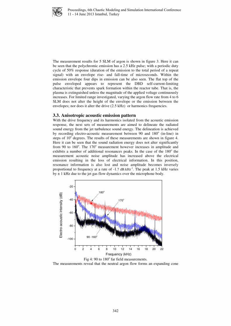
3.3. Anisotropic acoustic emission pattern With the drive frequency and its harmonics isolated from the acoustic emission
response, the next sets of measurements are aimed to delineate the radiated
sound energy from the jet turbulence sound energy. The delineation is achieved
by recording electro-acoustic measurement between 90 and 180o (in-line) in
steps of 10o degrees. The results of these measurements are shown in figure 4.
Here it can be seen that the sound radiation energy does not alter significantly
from 90 to 160o. The 170
o measurement however increases in amplitude and
exhibits a number of additional resonances peaks. In the case of the 180o the
measurement acoustic noise amplitude has increased above the electrical
emission resulting in the loss of electrical information. In this position,
resonance information is also lost and noise amplitude becomes inversely
proportional to frequency at a rate of -1.7 dB.kHz-1. The peak at 1.5 kHz varies
by ± 1 kHz due to the jet gas flow dynamics over the microphone body.
0 2 4 6 8 10 12 14 16 18 20 22
-100
-80
-60
-40
-20
180o
90 -160o
170o
Ele
ctr
o-a
co
ustic inte
nsity (
dB
)
Frequency (kHz) Fig 4: 90 to 180
o far field measurements.
The measurements reveal that the neutral argon flow forms an expanding cone
342

Proceedings, 6th Chaotic Modeling and Simulation International Conference
11 - 14 June 2013 Istanbul, Turkey
with internal angle of 10 degrees to the jet axis. This is in contrast to the 10 mm
in length visible pencil-like plasma plume, see figure 2 picture insert.
An investigation was carried out to determine the correlation between the area /
diameter treated by the kINPen MED gas plume and the water contact angle of
the PET placed under the jet. Measurements were obtained 1 hour after plasma
treatment as a function of the gap distance (5, 10, and 15 mm) between the jet
and the PET substrate. The contact angle obtained for the untreated PET was
85o. Table 1 shows the results of the measurements and the computed internal
cone angel for the treatment gap. This limited gap distance analysis reveals that
the treated diameter is much larger than the pencil-like diameter of the plasma
plume (~ 2 mm), with an overspill ratio (plasma/treatment diameter) of 8 to 10.
The treatment becomes less effective with gap distance. Correlating these results
with the acoustic mapping it appears that the argon gas passing through the
plasma zone and entering the expanding argon cone has a chemical ‘spillover
effect’on the surface properties of PET thus possibly differentiating between ion
exposure and radicals and metastable treatment mechanisms.
Table 1: PET WCA as a function gap distance. The photograph demonstrates
the increased water droplet width after the plasma treatment (2 mm scale bar).
No Plasma 5 mm 10 mm 15 mm 20 mm
WCA 85o 45
o 59
o 70
o
Overspill diameter N/A 16 mm 20 mm 18 mm
Treatment angle N/A 160 90 62
Overspill ratio N/A 8 10 9
4. Conclusion This paper examined the kINPen MED argon flow dynamics using
dimensionless analysis, electro-acoustic and photodiode measurements. The St
analysis of the plasma jet (with 5 other APPJs with similar nozzle diameters (D
= 1.7 to 4 mm) reveal similar nozzle oscillating flow mechanisms that produce
St values that are proportionally to Hz (0.6 to 0.9)
between 100 Hz to 1.1 MHz
where the rate is defined by the scale length of the nozzle. Electro-acoustic and
polychromic emission measurements reveal the APPJ nozzle is operating with a
low St < 0.5 for an argon flow of 4-6 SLM. The nozzle resonant frequency can
be modeled as a closed end column where resonance amplitude undergoes
amplification when plasma is applied. One possible mechanism for this acoustic
amplification may be due to electric winds [4] that are generated by the positive
and negative edges of the drive pulse and which are synchronized to the neutral
argon velocity to produce an enhanced molecular vibration at the nozzle exit.
The plasma jet therefore appears to act like a dielectric barrier discharge plasma
actuator. Electro-acoustic far field pattern measurements reveal an anisotropic
acoustic emission which is composed of sound radiation energy from the nozzle
and the axially aligned gas jet pressure. It has been shown that gas passing
343

Proceedings, 6th Chaotic Modeling and Simulation International Conference
11 - 14 June 2013 Istanbul, Turkey
through the visible plasma zone and entering the expanding argon cone alters
the hydrophobicity of PET when placed cone region.
Acknowledgement
This work is partially supported by Science Foundation Ireland Grant
08/SRCI1411 and the Enterprise Ireland Commercialisation Programme.
References 1. M. G. Kong, G. Kroesen, G. Morfill, T. Nosenko, T. Shimizu T, J. van Dijk and J. L.
Zimmermann. Plasma medicine: an introductory review, New J. Phys. 11, 115012,
2009.
2. M. Vandamme, E. Robert, S, Pesnel, S. Barbosa, S. Dozias, J. Sobilo, S. Lerondel, A.
Le Pape, J. M. Pouvesle. Antitumor Effect of Plasma Treatment on U87 Glioma
Xenografts: Preliminary Results, Plasma Processes and Polymers 7(3-4), 264-273,
2010.
3. K.-D. Weltmann, E. Kindel, R. Brandenburg, C. Meyer, R. Bussiahn, C. Wilke, and T.
von Woedtke. Atmospheric pressure plasma jet for medical therapy: plasma
parameters and risk estimation. Contrib. Plasma Phys. 49(9), 631-640, 2009.
4. M. Fitaire and T. D. Mantei. Some experimental results on acoustic wave propagation
in a plasma. Physics of Fluids. 15(3), 464-469, 1972.
5. V. J. Law, C. E. Nwankire, D. P. Dowling, and S Daniels. Acoustic emission within an
atmospheric helium discharge jet. Chaos Theory: Modeling, Simulation and
Applications. 255-264. Eds: C. H. Skiadas, I. Dimotikalis and C. Skiadas.
(Publisher: World Scientific 2011).
6. V. J. Law. Interdisciplinary Symposium on Complex Systems, 11-13th September
Prague, Czech Republic 2013.
7. V. J. Law, F. T. O’Neill and D. P. Dowling. Evaluation of the sensitivity of electro-
acoustic measurements for process monitoring and control of an atmospheric
pressure plasma jet system. PSST. 20(3), 035024, 2011.
8. V. J. Law, F. T. O’Neill, D. P. Dowling Atmospheric pressure plasma acoustic
moment analysis. Complex systems 20(2), 181-193 (Complex systems,
Publications, Inc 2011).
9. J. L. Walsh, F. Iza, N. B. Janson, V. J. Law and M. G. Kong. Three distinct modes in a
cold atmospheric pressure plasma jet. J, Phys, D: Appl, Phys 43(7), 075201 (14pp),
2010.
10. N. O’Connor and S. Daniels. Passive acoustic diagnostics of an atmospheric pressure
linear field jet including analysis in the time-frequency domain. J Appl. Phys 110,
013308, 2011.
11. V. F. Kopiev, V. A. Bityurin, I. V. Belyaev, S. M. Godin, M. Yu. Zaitsev, A. I.
Klimov, V. A. Kopiev, I. A. Moralev, and N. N. Ostrikov. Jet noise control using
the dielectric barrier discharge plasma actuators. Acoustical Physics. 58(4), 434-
441, 2012.
12. M. Samimy, J.-H. Kim, J. Kastner, I. Adamovich, and Y. Utkin. Active Control of a
Mach 0.9 Jet for noise mitigation using plasma actuators. AIAA J. 45( 4), 890-901,
2007.
13. J. F. Kolb, A. M. Mattson, C. M. Edelbute, X. H. Muhammad and L. C. Heller. Cold
dc-operated air plasma jet for the inactivation of infectious microorganisms. IEEE
PS 40(11), 3007-3026. 2012.
14. V. J. Law, M. Donegan and B. Creaven. Acoustic metrology: from atmospheric
plasma to solo percussive irish dance. CMSIM Journal. 4, 663-670, 2012.
344

Proceedings, 6th Chaotic Modeling and Simulation International Conference
11 - 14 June 2013 Istanbul, Turkey
1
Bursting Dynamics of Pancreatic β-cells
with Electrical and Chemical Couplings
Qishao Lu 1,
*, Pan Meng2
1) Department of Dynamics and Control, Beihang University, Beijing 100191,China
2) Department of Mathematics,Guangdong College of Pharmacy,Guangzhou 510224,China
* E-mail: [email protected]
Abstract: Pancreatic β-cells located in islets of Langerhans in the pancreas are responsible for the synthesis and secretion of insulin in response to a glucose challenge. Bursting electrical activity is also important for
pancreatic β-cells as it leads to oscillations in the intracellular free calcium concentration, which in turn leads
to oscillations in insulin secretion. The minimal model for a single pancreatic β-cell was extended by
introducing one additional ionic current was considered. The synchronization behaviors of two identical pancreatic β-cells connected by electrical (gap-junction) and chemical (synaptic) couplings, respectively, are
investigated based on bifurcation analysis by extending the fast-slow dynamics from single cell to coupled
cells. Various firing patterns are produced in coupled cells under proper coupling strength when a single cell
exhibits tonic spiking or square-wave bursting individually, no matter the cells are connected by electrical or chemical coupling. The above analysis of bursting types and the transition may provide us with better insight
into understanding the role of coupling in the dynamic behaviors of pancreatic beta-cells.
Keywords: Pancreatic β-cell, Coupling, Calcium oscillation, Bursting, Synchronization, Transition.
1. Introduction
Pancreatic β-cells located in islets of Langerhans in the pancreas are responsible for the synthesis
and secretion of insulin in response to a glucose challenge. Like nerve and endocrine cells,
pancreatic β-cells are electrically excitable and the electrical firing patterns typically come in the
form of bursting, characterized by an active phase of fast spiking followed by a quiescent phase
without spiking. It is well-known that bursting can be exhibited by a wide range of nerve and
endocrine cells and is likely one of the most important and distinctive firing patterns in dynamic
behaviors. Bursting electrical activity is also important for pancreatic β-cells as it leads to
oscillations in the intracellular free Ca2+
concentration, which in turn leads to oscillations in insulin
secretion.
2. The Model
The minimal model for a single pancreatic β-cell was extended by introducing one additional
ionic current, namely, the ATP-sensitive K+ current IK(ATP). This modified model described by
the following equations:
),(),(),()( )( pvIsvInvIvIdt
dvATPKskCa (1)
])([ nvndt
dn (2)
svsdt
dss )( (3)
Three variables in this system are the membrane potential (v), the delayed rectifier activation
(n), and a very slow variable s which has been postulated to be the intracellular Ca2+
.
Depending on the value of the parameter gs, the system either undergoes a spiking solution or
generates bursting oscillations, both of which can be explained by using fast-slow dynamics
analysis.
3. Main Results
The synchronization behaviors of two identical pancreatic β-cells connected by electrical
(gap-junction) and chemical (synaptic) couplings, respectively, are investigated based on
bifurcation analysis and numerical simulations by extending the fast-slow dynamics from
single cell to coupled cells. Various firing patterns are produced in coupled cells under proper
coupling strength when a single cell exhibits tonic spiking or square-wave bursting
345

Proceedings, 6th Chaotic Modeling and Simulation International Conference
11 - 14 June 2013 Istanbul, Turkey
2
individually, no matter the cells are connected by electrical or chemical coupling.
For two electrically coupled cells, when an isolated single cell exhibits continuous spiking
individually, with the coupling strength increasing, there exists synchronization transition
path including at least four different synchronous states, including two kinds of bursting
synchronization with totally different bifurcation structure of the fast subsystem, and another
two synchronous spiking regimes with continuous anti-phase and in-phase rhythms,
respectively.
For two chemically coupled cells, two spiking cells can transit to bursting under weak
chemical coupling condition. Moreover, an interesting inverse period-adding bursting
sequence is found when the isolated cell exhibits square-wave bursting. In addition, the two-
cell model with proper chemical coupling strength can produce the ―fold/Hopf‖ type of
bursting.
In summary,on the one hand, cells could burst synchronously for both weak electrical and
chemical couplings when an isolated single cell exhibits tonic spiking itself. Especially, for
electrically coupled cells, under the variation of the coupling strength there exist complex
transition processes of synchronous firing patterns, including the anti-phase continuous
spiking, then another type of bursting, and finally the in-phase tonic spiking. On the other
hand, it is shown that when an individual cell exhibit square-wave bursting, modest coupling
strength can make the electrically coupled system generate ―fold/Hopf‖ bursting via
―fold/fold" hysteresis loop while the chemically coupled system generate ―fold/Hopf‖
bursting. Especially, chemically coupled bursters could exhibit inverse period-adding bursting
sequence.
4. Conclusion
The above analysis of bursting types and the transition may provide us with better insight into
understanding the role of coupling in the dynamic behaviors of pancreatic β-cells. It is noticed
that these results are obtained when the slow variables of two cells are very near and could be
taken as the bifurcation parameter. In fact, this assumption is valid mostly except the inverse
period-adding bursting sequence occurring in the chemically coupled situation. The latter case
is worthy of further research.
References 1. F. Ashcroft and P. Rorsman. Electrophysiology of the pancreatic β-cell, Prog. Biophys.
Molec. Biol., vol. 54, 87—143 , 1989.
2. T. A. Krasimira, C. L. Zimliki, R. Bertram and A. Sherman. Diffusion of calcium and
metabolites in pancreatic islets: Killing osciaaltions with a pitchfork, J. Biophys., vol. 90,
3434-3446, 2006. 3. H. P. Meissner, Electrophysiological evidence for coupling between β-cells of pancreatic
islets, Nature, vol. 262, 502–504 , 1976.
4. A. Sherman and J. Rinzel. Model for synchronization of pancreatic beta-cells by gap
junctions, J. Biophys., vol. 59, 547-559 , 1991.
5. A. Sherman and J. Rinzel. Rhythmogenic effects of weak electrotonic coupling in
neuronal models, Proc. Natl. Acad. Sci. USA, vol. 89, 2471-2474, 1992.
6. A. Sherman. Anti-phase, asymmetric and aperiodic oscillations in excitable cells - I. Coupled
bursters, Bull. Math. Biol. vol. 56, 811–835, 1994.
7. D. Terman. The transition from bursting to continuous spiking in excitable membrane models,
J. Nonlinear Sci., vol. 2, 135–182, 1992.
8. E. M. Izhikevich. Neural excitability, spiking and bursting, Int. J. Bifur. and Chaos, vol. 10,
1171-1266 , 2000.
9. P. Meng, Q. S. Lu, and Q. Y. Wang, Dynamical analysis of bursting oscillations in the
Chay-Keizer model with three time scales, Science China: Series E, vol. 54, 1–9, 2011.
346
Proceedings, 6th Chaotic Modeling and Simulation International Conference
11 - 14 June 2013 Istanbul, Turkey
Chaos Cryptography: Relation Of Entropy With Message Length and Period
George Makris1 , Ioannis Antoniou2
Complex Systems Analysis Laboratory, Mathematics Department, Aristotle University, 54124, Thessaloniki, Greece 1E-mail: [email protected] 2E-mail: [email protected]
Abstract: Chaos cryptography is implemented by torus automorphisms with strictly positive entropy production. For any given entropy production 0h > we explicitly construct integer valued automorphisms with entropy ( )S ≥ . We identify compatibility conditions between the values of the entropy production and the lengths of the messages in terms of the grid size and we propose constructive ways to encrypt messages of arbitrary length in terms of torus automorphisms with any given desired entropy production. We moreover prove that the restrictions of chaotic maps with the same entropy have the same period for a fixed grid size. Keywords: Entropy, Cryptography, Chaos, Cryptography with Chaos. 1. Introduction Chaos cryptography was proposed by Shannon in his classic 1949 mathematical paper on Cryptography where used chaotic maps as models - mechanisms for symmetric key encryption. Of course Shannon did not employ the term Chaos which emerged in the 1970s. This remarkable intuition was based on the paradigm of the Baker’s map introduced by Hopf in 1934 as a simple deterministic mixing model with statistical regularity. Shannon observed that using chaotic maps, encryption is achieved via successive mixing of the initial information which is uniformly “spread” all over the available state space. In this way it is becoming exponentially hard to recover the initial message if the reverse transformation is not known. Baker’s map is the simplest example of chaotic Torus Automorphisms with constant Entropy production equal to one bit at every step. The Entropy production theory of Torus Automorphisms and general Chaotic maps was developed later by Kolmogorov and his group [Arnold and Avez, 1968; Katok ea, 1995; Lasota ea, 1994], following Shannon’s earlier foundation of Information Theory in 1948. Baker’s map has also served as a toy model for understanding the problem of Irreversibility in Statistical Mechanics [Prigogine, 1980]. Chaos cryptography with 2-dimensional maps deal with image encryption [Guan D. ea, 2005; Xiao G. ea , 2009] and text encryption [Kocarev ea, 2003; Kocarev ea, 2004; Kocarev L. and Lian S., 2011;Li S., 2003]. We have proposed a new implementation method for Chaos Cryptography based on Chaotic torus automorphisms, applicable for both image and text encryption simultaneously [Makris G, Antoniou I, 2012a] and designed torus automorphisms with desired entropy production [Makris G, Antoniou I, 2012b]. Part of these results is summatized in section 1.
347

Proceedings, 6th Chaotic Modeling and Simulation International Conference
11 - 14 June 2013 Istanbul, Turkey
As the grid discretizations of chaotic Torus automorphisms are periodic, for effective implementation we have to examine the conditions for reliable cryptography implementation. The objectives of this work are: a) to examine the dependence of the period on the entropy production and on the grid size (Section 2), b) to provide conditions for admissible grid discretizations (Section 3) and c) to provide algorithms for the construction of integer torus automorphims with desired entropy production (Appendix A) and for adapting the image size to the appropriate grid size (Appendix B) for customized implementation of chaotic cryptography). The automorphisms of the 2-torus [ ) [ )0,1 0,1Y = × are defined by the formula:
( )1
1
: : 1 , n n
n n
x xS Y Y A mod n
y y+
+
→ = ∈
(1)
Wherea b
Ac d
=
is a real invertible matrix with inverse:
1 d b1Ac aad bc
− − = − −
Chaotic Torus automorphisms (1) have one eigenvalue greater than 1, according Pesin’s 1977 Formula. Lemma:
1) The class of chaotic automorphisms (1) with ad bc 1− = consists of the matrices:
a b, , 0, 21 d
A a b d aadb
= ∈ ∈ − > −−
(2)
2) The entropy production of the Chaotic automorphisms (2) is:
( ) ( ) ( )2 1 2
2
2
2a d a d 4log log log
( ) ( ) 42 2
tr A tr Aλ
+ + + − + −= == ,
, , 2a b d a∈ ∈ > − (or ( ) 2tr A > ) (3)
3) The chaotic automorphisms (2) are expressed in terms of the entropy production as a parameter by the formula:
( )a b
, a , 0, 0a 2 2 a 12 2 a
A b
b
−−
= ∈ ∈ − >⋅ + − − + −
(4)
4) For the class of chaotic automorphisms Α with one eigenvalue greater than 1 and ad bc 1− = − we have the corresponding formulas:
348

Proceedings, 6th Chaotic Modeling and Simulation International Conference
11 - 14 June 2013 Istanbul, Turkey
a b, , 0, 1 d
A a b d aadb
= ∈ ∈ − > −+
(5)
( ) ( ) ( )
2 1 2
2
2
2a d a d 4log log log
( ) ( ) 42 2
tr A tr Aλ
+ + + += =
+ += ,
, ,a b d a∈ ∈ > − (or ( ) 0tr A > ) (6)
( )a b
, a , 0, 0a 2 2 a 12 2 a
A b
b
−−
= ∈ ∈ − >⋅ − − + − −
(7)
Formulas (2),(3),(4) are proven in [Makris G, Antoniou I, 2012b]. The corresponding formulas for the case ad bc 1− = − are obtained in a similar way. From formulas (3),(6) we see that Corollary Two Chaotic Torus Automorphisms have the same Entropy Production (are isomorphic), if and only if they have the same trace 2. Entropy production and the period of the discretization restrictions of integer Torus Automorphisms The implementation of cryptographic algorithms requires discretization of the chaotic maps onto the selected N N× grid. In order to preserve the grid structure we shall consider torus automorphisms with integer matrix elements. Given a desired entropy production value not less than h we may construct integer torus automorphisms with entropy production h from formulas (4),(7) using the algorithms presented in appendix A. The coordinates of pixels are elements of the NxN lattices N N× . The restriction of any integer torus automorphism to N N× (mod N):
( ) ( )'
mod mod'
x x a b xA N N
y y c d y
= =
(8)
is a periodic transformation, called the NxN discretization automorphism of (1). The period of the discretization automorphisms (8) is the minimal number T which satisfies the formula:
( ) 2
1 0mod
0 1
Ta bN
c d
= Ι =
(9)
Theorem 1: All discretization automorphisms (8) with the same trace have the same period T which depends only on the size N of the grid. Proof:
349

Proceedings, 6th Chaotic Modeling and Simulation International Conference
11 - 14 June 2013 Istanbul, Turkey
First we shall show that the discretization automorphisms (8) of isospectral matrices have the same period. It is enough to show that the matrices A (9) and
1
2
00λ
λ
∆ =
(10)
define discretization automorphisms (8) with the same period. We have:
1A B B−= ⋅∆ ⋅ Where B is a diagonalization transformation of A. If T is the period of (8), from (9) and (10) we have:
( )1 1TT TA B B B B− −= ⋅∆ ⋅ = ⋅∆ ⋅ and:
( ) ( )1 1
2
1 00mod mod
0 10
T T
T
a bN B B N
c dλ
λ−
= =
Therefore:
( )1
2
1 00mod
0 10
T
T Nλ
λ
=
Therefore the discretizations (8) of Δ and A have the same period T . From the eigenvalue formulas (3) and (6), we see that the eigenvalues 1 2,λ λ depend only on the trace of A. Therefore any two matrices with the same trace define discretizations (8) with the same period. 3. Entropy Production and Grid size We observe that torus automorphisms with different entropy production may have identical discretizations (8). For example, applying formula (6) we see that
the torus automorphisms with matrices 1
2 14093 2047
A =
and
2
2 193 47
A =
have entropy productions 1 11.0007h =
and 2 5.6141h = correspondingly. However their discretizations (8) to the grid 100 100× are identical:
2 1 2 1mod100 mod100
4093 2047 93 47
≡
.
The same is true for the grids 200 200× , 500 500× , 1000 1000× and others. This is an undesirable fact because only equivalent chaotic torus automorphisms should have identical grid discretization (8). We found that this requirement is true only for certain values of the entropy production h and grid size N . The result is the following:
350

Proceedings, 6th Chaotic Modeling and Simulation International Conference
11 - 14 June 2013 Istanbul, Turkey
Theorem 2: An necessary and sufficient condition for one to one correspondence between torus automorphisms and their grid discretizations (8) is: , ,max ,N a b c d> (11) Equivalently in terms of entropy production, using (3) and (6) we have the conditions:
( )a 2 2 a 1, ,x 2 ,ma 2h hN a b a
b
−−
⋅ + − − >
− +
for det( ) 1A = (12)
( )a 2 2 a 1, ,x 2 ,ma 2h hN a b a
b
−−
⋅ − − + >
− −
for det( ) 1A = − (13)
Prof:
( ) ( ) ( )( ) ( ) ( )
( )
mod modmod mod
mod mod
modb
c d
a N b Na b x xN N
c N d Nc d y y
xN
yαυ υυ υ
= =
=
As the remainders , , ,b c dαυ υ υ υ are always not greater than a,b,c,d
correspondingly, we have: bd
c d
a btr a d tr
c dα
α
υ υυ υ
υ υ
= + ≥ + =
Therefore, from (3) and (6) we have: b
c d
a bh h
c dαυ υυ υ
≥
b
c d
a bh h
c dαυ υυ υ
=
if and only if: a N< and b N< and c N< and d N< ,
from which follows the desired result. The natural question now arises what are the possible values of entropy production for automorphisms satisfying (11) Without significant loss of generality we consider the simpler class of integer torus automorphisms with 1b = . Formulas (12) and (13) are written :
( ) ( )22log 4 1 , 0h a N a N a N < + + + − − < <
, det( ) 1A = (14)
( ) ( )22log 4 1 , 0h a N a N a N < + + + + − < <
, det( ) 1A = − (15)
Therefore given the grid size N we know the maximal entropy production from (14),(15) for automorphisms with b=1 and conversely given a desired entropy production value we know the minimal grid size from (12),(13). The relation
351

Proceedings, 6th Chaotic Modeling and Simulation International Conference
11 - 14 June 2013 Istanbul, Turkey
between entropy production and grid size is shown in figure 1. We shall call the discretizations (8) with grid size N N× admissible discretizations if and only if the conditions (12) , (13) hold.
Entropy Production and Grid Size, det( ) 1A =
Entropy Production and Grid Size, det( ) 1A = −
0 5 10 15 200
1
2
3
4
5
6x 10
5 N(h) , a=N-1
h
N
0 5 10 15 20
0
1
2
3
4
5
6x 10
5 N(h) , a=N-1
h
N
Figure 1: Entropy Production and Grid Size
In case the grid N N× for admissible discretization (8) of the constructed torus automorphisms is larger than the message size n m× we may enlarge and adapt the message size to the grid size using the algorithm presented in appendix B. 5. Conclusions After extending our previous results [Makris G, Antoniou I, 2012b] on the entropy production on torus automorphisms (Lemma and Corollary), we show that the period of grid discretizations of chaotic automorphisms depends only on the entropy production and on the grid size (Theorem 1). In order to avoid the undesirable fact that torus automorphisms with different entropy production may have the same discretization, we provide a necessary and sufficient condition of admissible grid discretizations (Theorem 2). For customized implementation of chaotic cryptography, we provide algorithms for the construction of integer torus automorphims with desired entropy production (Appendix A) and for adapting the image size to the appropriate grid size (Appendix B). These results are necessary for implementation of chaotic cryptographic algorithms of desired entropy production. Based on Theorem 2 and Appendix B we can automatically adapt the message size to admissible discretization for effective cryptography. References 1. Akritas P., Antoniou I., Pronko G., "On the Torus Automorphisms: Analytic Solution,
Computability and Quantization", Chaos, Solitons and Fractals 12,(2001) 2805-2814 2. Arnold, V. I. and Avez, A., Ergodic Problems of Classical Mechanics Benjamin, New
York , 1968
352

Proceedings, 6th Chaotic Modeling and Simulation International Conference
11 - 14 June 2013 Istanbul, Turkey
3. Guan Z. H., Huang F., and Guan W.. Chaos-based image encryption algorithm. Physics Letters A, Vol. 346, Issues 1-3,( 2005), pp 153-157.
4. Dyson FJ, Falk H., Period of a discrete cat mapping. Am Math Monthly 1992;2(99):603-14
5. Hopf E., On Causality, Statistics and Probability, J. Math. and Phys. 13, (1934), 51-102.
6. Katok A., Hasselblatt B., Introduction to the Modern Theory of Dynamical Systems, Cambridge University Press, Cambridge, UK , 1995
7. Kocarev L., Sterjev M., Amato P., RSA ENCRYPTION ALGORITHM BASED ON TORUS AUTOMORPHISMS, IEEE, ISCAS (2004), IV 577-580.
8. Kocarev L., Tasev Z., and Makraduli J., “Public-Key Encryption and Digital-Signature Schemes Using Chaotic Maps”, 16th European Conference on Circuits Theory and Design, September 1 – September 4, 2003, Krakow, Poland, ECCTD 2003.
9. Kocarev, L., Lian, S., Chaos-Based Cryptography. Theory, Algorithms and Applications,Studies in Computational Intelligence, Vol. 354, (2011), ISBN 978-3-642-20542-2, Berlin.
10. Lasota A. and Mackey M., Chaos, Fractals, and Noise, Springer-Verlag New York, 1994.
11. Li, S., Analyses and New Designs of Digital Chaotic Ciphers. Ph.D. thesis, School of Electronic and Information Engineering, Xi’an Jiaotong University, Xi’an, China, 2003
12. Makris G., Antoniou I., 2012, "Cryptography with Chaos", Chaotic Modeling and Simulation (CMSIM), VOL 1: 169-178, 2012, ISSN 2241-0503.
13. Makris G., Antoniou I., 2012, "Cryptography with Entropy Producing Maps", 6th World Congress of NonLinear Analysts, IFNA 2012, 25 June - 1 July, Athens, Greece
14. Pesin Ya. B., Characteristic Lyapunov exponents and smooth ergodic theory, Russ. Math. Surv. 32:4, (1977), 55-112
15. Prigogine I., From Being to Becoming, Freeman, New York, 1980 16. Shannon C. , A Mathematical Theory of Communication. Bell System Technical
Journal, vol. 27, pp. 379–423, 623–656 (1948); Shannon C. and Weaver W., Mathematical Theory of Communication, Univ of Illinois Press, Urbana, Ill (1949).
17. Shannon, C., Communication Theory of Secrecy Systems. Bell System Technical Journal, Vol.28, Issue 4, (1949), pp 656–715.
18. Smale S., "Differentiable dynamical systems". Bulletin of the American Mathematical Society 73: (1967) 747–817.
19. Smale S., Finding a horseshoe on the beaches of Rio, Mathematical Intelligencer 20, (1998), 39-44
20. Xiao, D., Liao, X., Wei, P., Analysis and improvement of a chaos-based image encryption algorithm. Chaos, Solitons & Fractals, Vol. 40, Issue 5, (2009), pp 2191-2199.
353

Proceedings, 6th Chaotic Modeling and Simulation International Conference
11 - 14 June 2013 Istanbul, Turkey
Appendix A: Construction of integer torus automorphisms with entropy production not less than any desired positive real number Torus automorphisms have been applied to NxN grids and the periods has been related to the grid size N [Vivaldi, 1989; Dyson FJ and Falk H, 1992; Akritas ea, 2001;Antoniou ea, 1997; Xiao ea, 2009]. According to formula (2) we
should have a 1db−
∈ for any integer values a,b,d. , ie. : ( )a 1d mod b =
For any given entropy production 0h > we construct integer matrixes A with entropy ( )A ≥ according to the following algorithm. Algorithm 1. Construction of integer matrices A with ( )det 1A = Step 0: inputs: (0, ), a,∈ ∞ ∈ b
Step 1: Set ( ) 2 2x tr A − = = + , z is the ceiling of z
Step 2: Set d=x-a Step 3: if [ d>2-a and ( b=1 or (a ) 1d mod b = ) ] goto Step 9 Step 4: if [ a 0 and 0mod b b mod a≠ ≠ ] goto Step 7 Step 5: Set x=x+1 and d=x-a Step 6: goto Step 3 Step 7: Set a=a+1 and d=x-a Step 8: goto Step 3
Step 9: return a b
A 1 dadb
= −
Step 10: return λ1(A)=( ) ( )2a d a d 4
2+ + + −
Step 11: return ( ) ( )2 1logA Aλ=
Input Output
a b a b
A 1 dadb
= −
λ1(A) ( ) A
1.2 1 1 1 1
A1 2
=
2.6180 1.3885
1.2 2 3 2 3
A1 2
=
3.7321 1.9000
354

Proceedings, 6th Chaotic Modeling and Simulation International Conference
11 - 14 June 2013 Istanbul, Turkey
3.5 1 1 1 1
A10 11
=
11.9161 3.5748
3.5 5 1 5 1
A34 7
=
11.9161 3.5748
3.5 5 3 5 3
A13 8
=
11.9161 3.5748
11 2 1 2 1
A4093 2047
=
2049 11.0007
Table 1: Examples of Algorithm 1
According to formula (4) we should have a 1db+
∈ for any integer values
a,b,d. , ie. : ( ) ( )a 1 0 a 1d mod b d mod b b+ = ⇒ = −
Algorithm 2. Construction of integer matrices A with ( )det 1A = − Step 0: inputs: (0, ), a,∈ ∞ ∈ b
Step 1: Set ( ) 2 2x tr A − = = − , z is the ceiling of z
Step 2: Set d=x-a Step 3: if [ d>-a and ( b=1 or (a ) 1d mod b b= − ) ] goto Step 9 Step 4: if [ a 0 and 0mod b b mod a≠ ≠ ] goto Step 7 Step 5: Set x=x+1 and d=x-a Step 6: goto Step 3 Step 7: Set a=a+1 and d=x-a Step 8: goto Step 3
Step 9: return a b
A 1 dadb
= +
Step 10: return λ1(A)=( ) ( )2a d a d 4
2+ + + +
Step 11: return ( ) ( )2 1logA Aλ= Input Output
a b a b
A 1 dadb
= +
λ1(A) ( ) A
1.2 1 1 1 1
A2 1
=
2.4142 1.2716
355

Proceedings, 6th Chaotic Modeling and Simulation International Conference
11 - 14 June 2013 Istanbul, Turkey
1.2 2 3 2 3
A1 1
=
3.3028 1.7237
3.5 1 1 1 1
A12 11
=
12.0828 3.5949
3.5 5 1 5 1
A36 7
=
12.0828 3.5949
3.5 5 3 5 3
A12 7
=
12.0828 3.5949
11 2 1 2 1
A4093 2046
=
2048 11.0000
Table 2: Examples of Algorithm 2
Appendix B: Algorithm to Enlarge image size from ( )n m× to ( )N N× : Step 0: inputs: ( ), ,image N c , N: new image size, c: color of new pixels
Step 1: calculate ( ),n m =image size Step 2: hW N n= −
Step 3: Create an new blank image1 with size 2
hW m ×
and color c to every
pixel. Step 4: Create an new image2 with vertical quote of three images:
12
1
imageimage image
image
=
. Image2 size= ( )N m×
Step 5: wW N m= −
Step 6: Create a new blank image3 with size 2
wW N ×
and color c to every
pixel. Step 7: Create a new_image with horizontal quote of three images :
( )_ 3 2 3new image image image image= . new_mage size= ( )N N×
Image (342 x 454)
Image1 ( 79 x 454)
Image2 (500 x 454)
Image3 (500 x 23)
356

Proceedings, 6th Chaotic Modeling and Simulation International Conference
11 - 14 June 2013 Istanbul, Turkey
Inputs New_image
(500 x 500) Output
Image N=500 c=white Calculations
158hW N n == − 46wW N m= − =
New_image
The advantage of adding pixels in an image is to keep the original information.
357

Proceedings, 6th Chaotic Modeling and Simulation International Conference
11 - 14 June 2013 Istanbul, Turkey
358

Proceedings, 6th Chaotic Modeling and Simulation International Conference
11 - 14 June 2013 Istanbul, Turkey
Chaos Based Water Marked Image Encryption
Mahalinga V. Mandi, Dileep D
Dr. Ambedkar Institute of Technology, Bangalore, India
E-mail: [email protected]
Abstract: Digital image watermarking along with image encryption is a growing
research area. The use of chaos in image watermarking and image encryption algorithms
has seen tremendous advantages. In this paper a chaos based image watermarking to
provide authentication and chaos based watermarked image encryption to provide
security is proposed. The performance of the image watermarking and encryption is
mainly based on the randomness properties of chaotic binary sequences. Chaotic binary
sequences are derived from chaotic discrete sequences using logistic map equation. In
order for a complex imaging system to cope with these concerns, a cryptography
algorithm able to manage the vast amounts of data involved in image processing is
required. This paper proposes a new image watermarked encryption algorithm based on
Logistic map equation, in which the key space is 2212 which improves the security against
exhaustive attacks. Also good encryption speed is achieved using the proposed
algorithm. The experimental results and the security analysis including Key space,
Information entropy and key sensitivity proves that the proposed algorithm is secure,
authenticated and more efficient.
Keywords: Watermarking, Image encryption, Logistic map, Chaos
1. Introduction The growth of the digital technology and the associated need for information
integrity, authenticity and secrecy encourages the development of secure image
encryption systems. After the advent of the Internet and especially nowadays,
security of data and protection of privacy has become a major concern for
everyone‟s life. Combining the properties of cryptography and chaos theory it is
possible to design an image encryption algorithm that provides security,
authentication and privacy in image and video applications. Cryptography deals
with watermarking techniques to provide authentication and encryption
techniques to provide security. Chaos theory provides the suitable non linear
binary sequences that can be applied to watermarking and encryption algorithm.
Chaos is a deterministic, random like process found in non-linear, dynamical
system which is non-periodic, non-converging and bounded. Chaotic signals are
random like but they are produced by deterministic systems and can be
reproduced. Chaotic systems are sensitive to initial conditions and thus even
with a small difference in initial conditions will lead to the generation of very
different signals from the same dynamical system. The broad band, noise like
nature of chaos offers several advantages when used for generating key stream
for watermark and encryption algorithm. Chaotic sequences are non-repeatable;
if only part of the sequence is recovered then it is nearly impossible to
359

Proceedings, 6th Chaotic Modeling and Simulation International Conference
11 - 14 June 2013 Istanbul, Turkey
regenerate the whole sequence. This means that any unintended receiver
subjected to these sequences will encounter noise like waveforms whose
spectrum have no features that can be exploited for signal interception.
The chaos based image watermarking and encryption is discussed in [1] – [6]
and [12] – [13]. A watermarking procedure for digital image in the Complex
Wavelet Domain is discussed in [1]. The proposed watermark algorithm needs
three keys: a sub-image, a random location matrix and spread spectrum
watermark. The first and the second ones ensure the security of watermarking
procedure and the third one guarantees its robustness.
A new robust watermarking scheme based on a chaotic function and a
correlation method for detection, operating in the frequency domain is discussed
in [2]. This scheme is blind and comparing to other chaos related watermarking
methods, experimental results exhibit satisfactory robustness against a wide
variety of attacks such as filtering, noise addition, geometric manipulations and
JPEG compression with very low quality factors. The scheme also outperforms
traditional frequency domain embedding both in terms of robustness and
quality.
A digital image watermark algorithm based on discrete wavelet transform and
chaos theory is referred [3]. During the embedding of the watermarking, discrete
wavelet transform is done firstly and extract low frequency part as the
embedding field; then the chaotic sequence is used to encrypt the watermark and
transform the encrypted part and extract the low frequency; finally, embed the
low frequency part into that of the original image.
An efficient, secure color image coder incorporating Color-SPIHT (C-SPIHT)
compression and partial encryption is presented in [4]. Confidentiality of the
image data is achieved by encrypting only the significance bits of individual
wavelet coefficients for K iterations of the C-SPIHT algorithm. By varying K,
the level of confidentiality vs. processing overhead can be controlled.
A new approach for image encryption based on chaotic logistic maps in order to
meet the requirements of the secure image transfer is discussed in [5]. Here an
external secret key of 80-bit and two chaotic logistic maps are employed. The
initial conditions for the both logistic maps are derived using the external secret
key by providing different weightage to all its bits.
A digital image encryption algorithm four arry chaotic array is presented in [6]
and uses chaotic maps to generate four value chaotic array whose size as big as
image.
Combined with two chaotic maps, a novel alternate structure is applied to image
cryptosystem in paper [7]. A general cat-map is used for permutation and
diffusion, as well as the OCML (one-way coupled map lattice), which is applied
360

Proceedings, 6th Chaotic Modeling and Simulation International Conference
11 - 14 June 2013 Istanbul, Turkey
for substitution. These two methods are operated alternately in every round of
encryption process, where two sub-keys employed in different chaotic maps are
generated through the master-key spreading.
A paper on the utilization Pixels Arrangement and Random Permutation to
encrypt medical image for transmission security is presented in [8]. The
objective of this scheme is to obtain a high speed computation process and high
security. In this paper a new chaos based watermarked image encryption
algorithm is proposed. First the watermark is embedded in the image and then
the image is encrypted using two steps, first the image is position permuted and
then the substitution is done by XORring
each pixel. The key streams are
generated using logistic map equation.
The organization of the paper is as follows. Section 2 discusses the architecture
of the proposed scheme. Section 3 presents experimental results. Security
analysis is discussed in section 4. Finally the paper is concluded in section 5.
2. Architecture Fig. 1 shows the block diagram of chaos based image encryption scheme with
embedded watermark. In this diagram there are two parts. One that is used to
embed the watermark in the plain image using LSB insertion and the other that
encrypts the watermarked image using chaotic logistic map equation. LSB
insertion is randomly done and the LSB keystream is generated using chaotic
logistic map equation. The advantage of using LSB insertion is that it is possible
to embed a large watermark as compared to other techniques. In the
watermarked image encryption, mainly two steps are involved. First the image
is position permuted and then the substitution is done by Bitwise XORring
each
pixel with Key stream 3 to obtain an encrypted image. The Key stream 1 is used
for row permutation and Key stream 2 is used for column permutation.
Generation of Key streams is explained in Section 2.1.
Fig. 1. Proposed Encryption Scheme
Plain
Image
Position
Permutation
Encrypted
Authenticate
d Image
Key
Strea
m1
Key
Strea
m2
Key
Strea
m3
Bit-
wise
XOR
Chaos based
LSB
insertion
Watermark
LSB Key
Stream
Watermarked Image
361

Proceedings, 6th Chaotic Modeling and Simulation International Conference
11 - 14 June 2013 Istanbul, Turkey
Fig. 2 shows the watermark extraction. Here the decryption of the watermarked
image is exactly the reverse process and the same Key streams are used. The
watermark is also extracted with the same LSB Key stream. It is also possible to
know whether the watermark/image is tampered by comparing the extracted
watermark and the reference watermark. Hence the proposed algorithm not only
provides the required security but also provides the authentication.
Fig. 2. Watermark detection
2.1. Key stream generator
Key stream generator is as shown in Fig. 3. In this paper Logistic map is used
for generating chaotic real valued discrete sequence by selecting a key.
Fig. 3. Key Stream Generation
LSB Key
Stream
Reference
Watermark
Tampered
Image/
Watermark
Extracted
Watermark
Untampered
Image/Watermar
k
No
Yes
Encrypted
Authenticate
d Image
Position
Permutation
Decrypted
Authenticate
d Image
Key
Strea
m1
Key
Strea
m2
Key
Strea
m3
Bit-
wise
XOR
Chaos based Watermark
extraction
Compare
Logistic Map Binary
Conversion Key
Real valued discrete sequence
Key stream
Mapping Key Stream
362

Proceedings, 6th Chaotic Modeling and Simulation International Conference
11 - 14 June 2013 Istanbul, Turkey
The most commonly used chaotic map is Logistic map equation is given by,
x k+1 = r * x k * (1- x k) , 0 < x < 1 (1)
where x0 is the initial value, r is the bifurcation parameter and depending on the
value of r, x0 the dynamics of the generated chaotic sequence can change
dramatically. For 3.57 < r ≤ 4, the sequence is found to be non periodic and non-
converging [9]. The probability density function of Logistic map is symmetric
and hence the binary conversion is done as shown in equation (2).
bi = 0 for xk < 0.5
and bi = 1 for xk ≥ 0.5 (2)
where 0 < i < n , n = length of the chaotic sequence.
Key = key1, key2, key3 is composed of three sub-keys, where sub-key1 is
used as initial value for generating key stream1, sub-key2 is used as initial value
for generating key stream2 and sub-key3 is used as initial value for generating
key stream3. Key stream mapping for generating key stream1, 2 and 3 are as
shown in Fig. 4.
Fig. 4. Key Stream Mapping
Where B1, B2…etc denotes decimal numbers obtained by combining k-binary
numbers for each streams respectively. Thus if the Image to be encrypted is of
size 2M
X 2N then required length of key Stream 1 which is used for row
permutation is 2
M and the range is [0, 2
M -1], required length of key Stream 2
used for column permutation is 2N
and the range is [0, 2N -1] and the required
length of key Stream 3 which is used for bitwise XORring
is 2M
X 2N X 8 and
the range is [0, 255].
During the key stream 1 and 2 generation, it must be guaranteed that there is no
duplicate element in the two streams by discarding the repeated sequence.
The LSB key stream is similar to key stream 3 and mainly depends on the size
of the watermark.
3. Experimental Results In order to test this algorithm we considered standard 512 X 512 Lena bmp
image. In this Lena image a watermark „R‟ of size 14 X 14 is embedded. The r
363

Proceedings, 6th Chaotic Modeling and Simulation International Conference
11 - 14 June 2013 Istanbul, Turkey
value is taken as 3.99 and the initial values to generate key streams 1, 2 and 3
respectively is taken as key = key1, key2, key3 = 0.6532245, 0.9874562,
0.416745. For generating the LSB key stream the initial value is taken as
0.62343242.
Fig. 5 shows the input image, watermark embedded image, watermark and
watermark extract.
Fig. 5. Input image and Watermark
Fig. 6 to Fig. 9 shows the histogram of the input image, encrypted image,
encrypted image histogram and decrypted image respectively.
Fig. 6. Input Image Histogram Fig. 7. Encrypted Image
Encrypted Image
0
500
1000
1500
2000
2500
3000
Input Image Histogram
0 50 100 150 200 250
Input Image Watermarked Image
Watermark Watermark Recovered
364

Proceedings, 6th Chaotic Modeling and Simulation International Conference
11 - 14 June 2013 Istanbul, Turkey
Fig. 8. Encrypted image histogram Fig. 9. Decrypted image
The encryption and Decryption time in Matlab for a 512 X 512 bmp image was
found to be 0.679 seconds.
4. Security Analysis A good encryption schemes should resist all kinds of known attacks such as
known/chosen plain text attacks, cipher text only attack, statistical attack and
various brute force attacks. We will present some security analysis on the
proposed encryption scheme in this section.
4.1. Key space analysis Considering most commonly used PC platform as an example, the computation
precision is 16 decimal digits, therefore a chaos-based cryptosystem can only
provides 1016
≈253
size key space [10], which is a little smaller than DES(256
)
and by far smaller than AES(2128
). Since key = key1, key2, key3 and LSB key
which is composed of four sub-keys, the key space size is (1016
)4 ≈ 2
212, which is
larger than the acknowledged most security AES algorithm. Besides, the scheme
is secure against known/chosen-plaintext attack, since it adopts both
permutation and substitution operations.
4.2. Information entropy Entropy of a random image source is expected to be eight for an image in which
each pixel is 8-bits [11]. The entropy of the input image in was found to be
7.3465 and the entropy of the encrypted image was found to be 7.9963, which is
very close to the theoretical value. The entropy of the encrypted image of the
proposed scheme is very close to the ideal one. Also the entropy of the
watermarked image is equal to 7.3466 which is almost same as that of the input
image.
Decrypted Image
0
500
1000
1500
2000
2500
Encrypted Image Histogram
0 50 100 150 200 250
365

Proceedings, 6th Chaotic Modeling and Simulation International Conference
11 - 14 June 2013 Istanbul, Turkey
4.3. Key Sensitivity A good crypto-system should be sufficiently sensitive to small changes in the
key. In the proposed scheme with a small change in the key it is not possible to
decrypt the image. This was observed by selecting the key = 0.6532245,
0.9874562, 0.41674500001 and by decrypting the image with a
wrong key, key3 is not possible. Fig. 10 shows the decrypted image with a
wrong key and its histogram.
Fig. 10. Decrypted image and its histogram with a wrong key
5 Conclusions In this paper a new a good performance chaos based security algorithm for
images is proposed. The algorithm proposed in this paper provides security as
well as authenticity. The advantage of this algorithm is that the key space is
enlarged to 2212
, which improves the security against exhaustive attack and also
the good encryption speed which is enhances the performance when image size
is large. The entropy of the encrypted image of the proposed scheme is very
close to the ideal one and hence the encrypted image appears to be highly
random which is observed from the histogram of encrypted image. The
simulation result shows that the proposed scheme has very good key sensitivity
which provides good security for color images. By comparing the extracted
watermark with the reference watermark it is easy to find whether the
image/watermark is tampered or not.
Acknowledgement The authors would like to thank the Principal, Management, SPFU and NPIU
for sponsoring the authors to present the paper in the International Conference
CHAOS 2013 under the World Bank Funded Project TEQIP-2.
References 1. S. Mabtoul , E. Ibn-Elhaj , D. Aboutajdine, “A Blind Chaos-Based Complex
Wavelet-Domain Image Watermarking Technique”, Proc. Int Jnl. of Computer
Science and Network Security, VOL.6 No.3, pp. 134-139, March 2006
366

Proceedings, 6th Chaotic Modeling and Simulation International Conference
11 - 14 June 2013 Istanbul, Turkey
2. E. Chrysochos, V. Fotopoulos, and A. N. Skodras, Robust Watermarking of Digital
Images Based on Chaotic Mapping and DCT”.
3. Qiang Wang, Qun Ding, Zhong Zhang and Lina Ding, “Digital Image Encryption
Research Based on DWT and Chaos”, Proc. Fourth IEEE Int. Conf. on Natural
Computation, pp. 494-498, 2008.
4. Karl Martin, Rastislav Lukac, Konstantinos N. Plataniotis, “Efficient encryption
ofwavelet-based coded color images”, Jnl. Pattern Recognition Society, Elsevier,
pp. 1111 – 1115, 2006.
5. N.K. Pareek, Vinod Patidar, and K.K. Sud, “Image encryption using chaotic logistic
map”, Jnl. Image and Vision Computing, Elsevier, pp. 926–934, 2006.
6. Gao Shan-qing, Zhang Shi-jie, Liu Bin, Luo Xiang-yang and Liu Fen-lin, ” An
Image Encryption Algorithm based on Four-value Chaotic Array”, Jnl. Image and
Graphics, Vol. II, No. 2, pp. 244-250, Feb. 2006.
7. Zhang YiWei1, Wang YuMin & Shen XuBang, “A chaos-based image encryption
algorithm using alternate structure”, Springer, Vol. 50, No. 3, pp. 334-341, June
2007.
8. Koredianto Usman, Hiroshi Juzoji, Isao Nakajima, Soegijardjo Soegidjoko,
Mohamad Ramdhani, Toshihiro Hori and Seiji Igi, “Medical Image Encryption
Based on Pixel Arrangement and Random Permutation for Transmission Security”,
IEEE, pp. 244-247, 2007.
9. Mahalinga V.Mandi, R. Murali K.N.Haribhat,” Chaotic functions for generating
binary sequences and their suitability in Multiple Access”, Proc. IEEE-ICCT
2006,Vol. 1,pp.217-220.
10. Chong Fu,Zhiliang Zhu, ”A Chaotic Image encryption scheme based on circular bit
shift method”, The 9th International Conference for Young Computer Scientists,
IEEE Computer Society, pp. 3057 – 3061, 2008.
11. Xu Shu-Jiang, Wang Ying-Long, Wang Ji-Zhi, Tian Min,” A Novel Image
Encryption Scheme Based on Chaotic Maps”, Proc. IEEE-ICSP 2008, pp. 1014 –
1018.
12. Soumaya Al-Maadees, Afnan Al-Ali and Turki Abdalla, “A New Chaos-Based
Image-Encryption and Compression Algorithm”, Journal of Electrical and Computer
Engineering, Volume 2012 (2012), Article ID 179693, 11 pages,
DOI:10.1155/2012/179693.
13. Chen Zaiping, Li Haifen, Dong Enzeng and Du Yang, “Hyper-Chaos Based Image
Encryption Algorithm”, 2nd IEEE International Conference on Intelligent Human-
Machine Systems and Cybernetics (IHMSC), 2010, Volume: 2, pp. 188 – 191.
367

Proceedings, 6th Chaotic Modeling and Simulation International Conference
11 - 14 June 2013 Istanbul, Turkey
368

Proceedings, 6th Chaotic Modeling and Simulation International Conference
11 - 14 June 2013 Istanbul, Turkey
1
Maximova Marina
South-Russian State Technical University (Novocherkassk Polytechnic Institute), Faculty of Socio-
Humanitarian Knowledge, Department of Philosophy
Email: [email protected]
An attractor and a superattractor in the contemporary
pan-humanitarian space
Abstract: The work purpose is clearing up the possibility of adequate use of the
applied synergetics results in the sphere of philosophical and social knowledge. On
the basis of the contemporary Russian researchers' works the author analyzes the
concept of an attractor and a superattractor as the goal of a complex system,
considers prospects of synergetics methodology use in the epistemological scientific
field.
Keywords: attractor, superattractor, synergetics, socio-humanitarian systems, post-
nonclassical paradigm
1. Introduction: One of the major defining concepts in the contemporary
synergetics, namely the attractor, can be developed in the area of both applied and
abstract and philosophical knowledge. An attractor as an emergent formation shows
qualitative changes in the process of evolutionary development of any system,
including non-natural, general social systems. According to the author, an attractor
represents a system innovation [1,2], - a conceptual change in the system which
radically alters its behaviour.
For more "evident" confirmation of the idea the author offers to use the Darwinian
concept of selection which if applied to socio-humanitarian systems is interpreted as
occurrence of bifurcation points, branching of the system associated with
uncertainty in its further development when the most suitable variant satisfying the
"natural" laws of development defines further vector of movement. The system
evolution process is a process of movement on the way chosen in the bifurcation
point. Thus, the universal mechanism of evolution is revealed at the moment of
bifurcation by selecting structures capable of bringing the system to a totally new
level. An attractor, or an innovation is a conceptual change most suitable for novelty
features. Such an attractor represents rather stable state of the system, a balance
between instability and steady state.
2. Essence of the attractor in socio-humanitarian systems. In comparison with
applied synergetics, use of synergetic methodology in humanitarian knowledge has
a number of peculiarities. In particular, social systems have a higher level of
complexity as they include "the human" factor, namely a role of a man as the
subject of knowledge. Taking into account such a feature of «human» systems it is
offered to consider the attractor to be not a point but K. Lorenz's strange attractor
having a limited area of its existence, a certain field of possible decisions. If, by
analogy with applied synergetics, the attractor is understood to be the system goal, it
will allow to show pluralistic character of social processes with a great number of
various goals at different levels of the action.
Laws of social systems functioning are associated with processes of apprehending
by the subject the activity results in its total variety. In this case it is inevitably
necessary to touch upon the question on the goal essence and on necessity of its
understanding change according to scientific trends of the postnonclassical
scientific paradigm. If we understand the social system goal to be the strange
attractor, it is necessary to reveal its features in this context.
369

Proceedings, 6th Chaotic Modeling and Simulation International Conference
11 - 14 June 2013 Istanbul, Turkey
2
First, it is necessary to note conventionality of the concept of the local goal of self-
organizing systems of any nature. The concept of the goal assumes availability of an
external subject which sets this goal. Sinergetic systems of such a subject do not
have and cannot have. Therefore, in accordance with the results of the researches
[3], complex self-organizing systems of a social nature can be referred to the group
of teleonomic systems. These are systems which evolve to some final condition
without a specific initial programme.
In this case, the concept of "the goal" can be defined as an internally determined
condition of a social system and a direction of its change and development, that is
the system trend to the order. In the process of evolutionary development the similar
"goal" reasons play the increasing role, accordingly the factors named the order
parametres, become complicated as well. Along with their complication, the
system “goals” become more complicated, their quantity set by the strange attractor
increases.
Every social attractor forms its area of attraction, therefore intrasystem relations
based on coherent collective movement of the system components arise.
3.A superattractor and its meaning in the contemporary reality. According to
N.I. Moiseyev [4], a social system can have a great number of attractors. Proceeding
from it, it is logical to differentiate local attractors as intermediate goals of
evolutionary processes, and global, that is consolidating the whole process of the
system functioning. Taking into account complexity of non-natural systems, it
seems to be pertinent to clear up social parametres of such a global attractor as a
goal-like structure.
In this connection Russian scientist V.P. Bransky [5] determines the concept of a
superattractor. A superattractor is fundamentally important when considering social
systems as it defines availability of the global "goal" of the whole system which
can be understood as a general meaning of the evolution. A global attractor (a
superattractor) can be presented as an asymptotically stable point in the evolution
spiral which movement incessantly approaches this point.
The incessant aiming for a superattractor is caused by complexity of its nature, non-
linearity of movement to it. In the interpretation of social processes V.P. Bransky
understands a superattractor as a limit of the mankind cultural development, a
meaning of global self-organization, the order and chaos synthesis, more precisely,
the order which is stable against the chaos.
The concept of a superattractor defines the system integrity, representing the
concept of holistic synergistic system world outlook.
According to V.P. Bransky, a superattractor is a much broader category in
comparison with the concept of the system goal. In the conception of synergistic
historicism [5] a superattractor is interpreted as a public ideal and analyzed
particularly from the view point of its subjective spiritual characteristics associated
with axiological categories. According to such conception, the most general concept
concerning social processes is the concept of the ideal including a number of value
and world outlook characteristics.
From this view point the ideal acquires a global comprehensive character. V.P.
Bransky notes that in the XX-th century philosophy there was a trend to replace the
concept of "the ideal" with the concepts of "the project", "the plan" that does not
correspond to global essential characteristics of the ideal – a superattractor
including all the scale of axiological categories, such as value, meaning, truth, as
well as a doubtless strategic component.
Taking into account the complex nature of a superattractor in social systems, in my
opinion, it is pertinent to make emphasis on understanding of a superattractor as the
global goal of the system dealing with world outlook and value systems in the social
processes. In this case the term "the ideal" in the best way possible corresponds to
such a concept including complex subjective social characteristics.
370

Proceedings, 6th Chaotic Modeling and Simulation International Conference
11 - 14 June 2013 Istanbul, Turkey
3
So, from the view point of synergetics and the conception offered by V.P. Bransky,
development can be interpreted as the directed non-linear movement to a
superattractor fulfilled through the change of local attractors by means of self-
organization.
For example, for today, such a broad social phenomenon as globalization can be
understood, proceeding from the synergistic paradigm, as a social self-organization
of the wide range.
The concept of a global superattractor of the social system is used as a consolidating
parametre uniting the scope of self-organization processes at various being levels
and determiming the evolution in its integrity. On this basis the contemporary
synergistic world outlook becomes truly holistic: any object is as the universal
component which "strives" for a superattractor.
4. Conclusion. Defining an attractor as one of the crucial concepts of the
contemporary synergetics in the pan-humanitarian supplement is caused by its goal-
like behaviour and backbone characteristics. In this context the concept of «a
superattractor» offered by the Russian philosophical school, which allows to
interpret the unified process of the universal evolution from the view point of the
synergistic methodology is challenging.
References:
1.Maksimova M.V. Innovation and synergistic reconstruction of evolutionary
epistomology S. Tulmina. Scientific thought of the Caucasus.- 2010,- No. 1, pp.56-
60
2.Maksimova M.V. Innovations in synergetics of socio-humanitarian processes.
CHAOS 2009 : Chaotic Modeling and Simulation : Books of Abstracts International
Conference, Chania Crete Greece, June 1-5, 2009 / Editor Christos H. Skiadas.-
Chania Crete Greece, 2009.- p.47
3.Mamchur E.N. Spontaneity and teleologism. Spontaneity and determinism.
Institute of Philosophy at the Russian Academy of Sciences. – М.: Nauka, 2006. –
pp. 225–248.
4.Moiseyev N.N. Farewell to simplicity / N.N. Moiseyev. – М.: Agraf, 1998. – p.
474.
5.Bransky V.P. Globalisation and synergistic historicism. St. Petersburg:
Politekhnika, 2004. – p. 400.
371

Proceedings, 6th Chaotic Modeling and Simulation International Conference
11 - 14 June 2013 Istanbul, Turkey
372

Proceedings, 6th Chaotic Modeling and Simulation International Conference
11 - 14 June 2013 Istanbul, Turkey
Weak Regularized Solutions to StochasticCauchy Problems⋆
Irina V. Melnikova1 and Uljana A. Alekseeva2
1 Ural Federal University, Institute of Mathematics and Computer Sciences, 620083Ekaterinburg, Lenina av., 51, Russia(E-mail: [email protected])
2 Ural Federal University, Institute of Mathematics and Computer Sciences, 620083Ekaterinburg, Lenina av., 51, Russia(E-mail: [email protected])
Abstract. The Cauchy problem for systems of differential equations with stochasticperturbations is studied. Weak regularized solution are constructed for the case ofsystems with operators generating R-semigroups; generalized and mild solutions areintroduced.Keywords: white noise process; Wiener process; weak, regularized, generalized andmild solutions; Gelfand-Shilov spaces.
1 Introduction
Let (Ω,F , P ) be a random space. We consider the Cauchy problem for thesystems of differential equations with stochastic perturbations :
∂X(t, x)
∂t= A
(i∂
∂x
)X(t, x) +BW(t, x), t ∈ [0, T ], x ∈ R, (1)
X(0, x) = f(x), (2)
where A(i ∂∂x
)is a matrix operator: A
(i ∂∂x
)=
Ajk
(i ∂∂x
)m
j, k=1generating
different type systems in the Gelfand-Shilov classification [3], Ajk
(i ∂∂x
)are lin-
ear differential operators in L2(R) of finite orders; W = W(t), t ≥ 0 is a ran-dom process of white noise type in Ln
2 (R): W(t) = (W1(t, x, ω), . . .W1(t, x, ω)),x ∈ R, ω ∈ Ω; B is a bounded linear operator from Ln
2 (R) to Lm2 (R); f is an
Lm2 (R)-valued random variable; X = X(t), t ∈ [0, T ] is an Lm
2 (R)-valuedstochastic process X(t) = (X1(t, x, ω), . . . Xm(t, x, ω)), x ∈ R, ω ∈ Ω, which isto be determined.
This problem usually is not well-posed for several reasons. The first oneis caused by the fact that the differential operators A
(i ∂∂x
)generally do not
generate semigroups of class C0 and the corresponding homogeneous Cauchyproblem is not uniformly well-posed in Lm
2 (R), they generate only some regu-larized semigroups. By this reason we look for a regularized solution of (1)–(2).The second reason is the irregularity of a white noise process, because of thiswe need to consider not the original equation (1) but the integrated one, that is
⋆ The work was supported by the Ministry of Education and Science of RussianFederation (Program 1.1016.2011) and by RFBR, project 13-01-00090
373

Proceedings, 6th Chaotic Modeling and Simulation International Conference
11 - 14 June 2013 Istanbul, Turkey
an equation in the Ito form with a Wiener process W being a kind of primitiveof white noise W:
X(t, x) = f(x) +
∫ t
0
A
(i∂
∂x
)X(τ, x) dτ +BW (t, x), t ∈ [0, T ], x ∈ R. (3)
In addition, we can not expect the stochastic inhomogeneity be in the domainof A
(i ∂∂x
), by this reason we have to explore weak regularized solutions to the
integrated problem (3).
2 Necessary definitions and preliminary results
We consider the problem (1)–(2) as an important particular case of the abstractCauchy problem
X ′(t) = AX(t) +BW(t), t ∈ [0, T ], X(0) = f, (4)
and the problem (3) as that of the abstract integral one (written as usually inthe form of differentials):
dX(t) = AX(t)dt+BdW (t), t ∈ [0, T ], X(0) = f, (5)
with A being the generator of a regularized semigroup in a Hilbert space H, es-pecially an R-semigroup (see, exp., Melnikova[4], Melnikova and Anufrieva[6]).Thus, we continue investigations of Da Prato[2], Melnikova et al. [5], Alshan-skiy and Melnikova[1]. We assume in this paper H = Lm
2 (R).
Definition 1. Let A be a closed operator and R be a bounded linear operatorin Lm
2 (R) with a densely defined R−1. A strongly continuous family S :=S(t), t ∈ [0, τ), τ ≤ ∞, of bounded linear operators in Lm
2 (R) is called anR-regularized semigroup (or R-semigroup) generated by A if
S(t)Af = AS(t)f, t ∈ [0, τ), f ∈ domA, (6)
S(t)f = A
∫ t
0
S(τ)f ds+Rf, t ∈ [0, τ), f ∈ Lm2 (R). (7)
The semigroup is called local if τ < ∞.
Definition 2. LetQ be a symmetric nonnegative trace class operator in Ln2 (R).
An Ln2 (R)-valued stochastic process W (t), t ≥ 0 is called a Q-Wiener process
if(W1) W (0) = 0 Pa.s. ;(W2) the process has independent increments W (t)−W (s), 0 ≤ s ≤ t,
with normal distribution N (0, (t− s)Q);(W3) W (t) has continuous trajectories Pa.s.
Definition 3. Let Ft, t ≤ ∞ be a filtration defined by W . An Lm2 (R)-valued
Ft-measurable process X = X(t), t ∈ [0, T ] is called a weak R-solution of
374

Proceedings, 6th Chaotic Modeling and Simulation International Conference
11 - 14 June 2013 Istanbul, Turkey
the problem (3) with A(i ∂∂x
)generating an R-semigroup S(t), t ∈ [0, τ) in
Lm2 (R) if the following conditions are fulfilled:
1) for each t ∈ [0, T ], k = 1,m,∫ t
0∥Xk(·, τ)∥L2(R) dτ < ∞ Pa.s.;
2) for each g ∈ domA∗, X satisfies the weak regularized equation :
⟨X(t), g⟩ = ⟨Rf, g⟩+∫ t
0
⟨X(τ), A∗g⟩ dτ + ⟨RBW (t), g⟩ Pa.s. , t ∈ [0, T ]. (8)
It is proved by Melnikova and Alshanskiy[1] that a weak R-solution of theabstract stochastic Cauchy problem (5) with densely defined A being the gener-ator of an R-semigroup and W being a Q-Wiener process exists and is unique.In our case of the problem (3) we have the following result.
Theorem 1. Let W (t), t ≥ 0 be a Q-Wiener process in Ln2 (R) and A
(i ∂∂x
)be the generator of an R-semigroup S(t), t ∈ [0, τ) in Lm
2 (R) satisfying thecondition ∫ t
0
∥S(τ)B∥2HS dτ < ∞, (9)
where ∥ · ∥HS is the norm in the space of Hilbert-Schmidt operators acting from
the space Q12Ln
2 (R) to Lm2 (R). Then for each F0-measurable Lm
2 (R)-valuedrandom variable f
X(t) = S(t)f +
∫ t
0
S(t− τ)B dW (τ), t ∈ [0, T ], (10)
is the unique weak R-solution of (5).
We see in (10) that the main part of constructing an R-solution is con-structing an R-semigroup generated by A. It is not an easy task to constructR-semigroups generated by given operators A in the general case. But for dif-ferential operators A
(i ∂∂x
)such semigroups can be constructed and we describe
a way to do this in the present paper.Our methods are based on investigations of the differential systems:
∂u(t, x)
∂t= A
(i∂
∂x
)u(t, x), t ∈ [0, T ], x ∈ R, (11)
provided by the generalized Fourier transform technique in [3]. So, let us applythe Fourier transform to the system (11) and consider the dual one:
∂u(t, s)
∂t= A(s)u(t, s), t ∈ [0, T ], s ∈ C. (12)
Let the functions λ1(·), . . . , λm(·) be characteristic roots of the system (12)and Λ(s) := max
1≤k≤mℜλk(s), s ∈ C. Then solution operators of (12) have the
following estimation
etΛ(s) ≤∥∥∥etA(s)
∥∥∥m
≤ C(1 + |s|)p(m−1)etΛ(s), t ≥ 0, s ∈ C. (13)
375

Proceedings, 6th Chaotic Modeling and Simulation International Conference
11 - 14 June 2013 Istanbul, Turkey
Definition 4. A system (11) is called1) correct by Petrovsky if there exists such a C > 0 that Λ(σ) ≤ C, σ ∈ R;2) conditionally–correct if there exist such constants C > 0, 0 < h < 1,
C1 > 0 that Λ(σ) ≤ C|σ|h + C1, σ ∈ R;3) incorrect if the function Λ(·) grows for real s = σ in the same way as for
complex ones: Λ(σ) ≤ C|σ|p0 + C1, σ ∈ R.
Finally, note that the operator i ∂∂x is self-conjugate in L2(R):
(i ∂∂x
)∗= i ∂
∂x .Hence the differential operator of (1) has the following conjugate one
A∗(i∂
∂x
)=
Akj
(i∂
∂x
)m
k,j=1
,
obtained of Ajk
(i ∂∂x
)mj,k=1 by replacing components with conjugate operators
and by further transposition.
3 Construction of R-semigroups generated by A(i ∂∂x
)Since for the problem (12) solution operators of multiplication by etA(·), t ≥ 0,generally have an exponential growth (13), one can not obtain propagators ofthe problem (11) in the framework of the classical inverse Fourier transform.That is why we introduce an appropriate multiplierK(·) into the inverse Fouriertransform :
GR(t, x) :=1
2π
∫ ∞
−∞eiσxK(σ)etA(σ) dσ, (14)
providing the uniform convergence of this integral with respect to t ∈ [0, T ] inLm2 (R)× Lm
2 (R) =: Lm2 . For this purpose we require K(·)etA(·) ∈ Lm
2 .The matrix-function GR(t, x) obtained in (14) is a regularized Green func-
tion. If its convolution with f is well-defined, then the convolution gives aregularized solution of (11). In addition to the above condition, we introduceK(·) providing∫ ∞
−∞eiσxK(σ)etA(σ)f(σ) dσ ∈ Lm
2 (R), t ∈ [0, T ], (15)
for each f ∈ Lm2 (R). These conditions hold, for example, if K(·)etA(·) ∈ Lm
2
and is bounded.Now we show that the family of convolution operators with GR(t, x):
(S(t)f)(x) := GR(t, x) ∗ f(x), t ∈ [0, τ), (16)
forms a local R-semigroup in Lm2 (R) for any τ < ∞. To begin with, we verify
the strong continuity property of the family S(t), t ∈ [0, T ], T < ∞ : forarbitrary f ∈ Lm
2 (R) we show that ∥S(t)f − S(t0)f∥Lm2 (R) → 0 as t → t0.
∥S(t)f − S(t0)f∥2Lm2 (R) =
376

Proceedings, 6th Chaotic Modeling and Simulation International Conference
11 - 14 June 2013 Istanbul, Turkey
=
∫R
(1
2π
∫ ∞
−∞eiσxK(σ)
[etA(σ)f(σ)− et0A(σ)f(σ)
]dσ
)2
dx.
Let us split the inner integral into the three integrals:∫|σ|≥N
eiσxK(σ)etA(σ)f(σ) dσ −∫|σ|≥N
eiσxK(σ)et0A(σ)f(σ) dσ
+
∫|σ|≤N
eiσxK(σ)[etA(σ) − et0A(σ)
]f(σ) dσ. (17)
Note that the functions hN (x, t) :=
∫|σ|≥N
eiσxK(σ)etA(σ)f(σ) dσ and
gN (x, t) :=
∫|σ|≤N
eiσxK(σ)[etA(σ) − et0A(σ)
]f(σ) dσ
are elements of Lm2 (R) for all t ∈ [0, T ] as the inverse Fourier transform of the
functions from Lm2 (R)
hN (σ, t) =
0, |σ| ≤ N,
K(σ)etA(σ)f(σ), |σ| > N,
and gN (σ, t) = K(σ)etA(σ)f(σ) − hN (σ, t), respectively. Further, since
K(·)etA(·) ∈ Lm2 and f(·) ∈ Lm
2 (R), the integral (15) is convergent uniformlywith respect to x ∈ R and t ∈ [0, T ], then for any ε > 0
|hN (x, t)| < ε/4, x ∈ R, t ∈ [0, T ],
by the choice of N . So, sum of absolute values of the first two integrals in (17)is less than ε/2. Now fix N . Since
(e(t−t0)A(σ) − 1
)→ 0 as t → t0 uniformly
with respect to σ ∈ [−N,N ], we can take
|gN (x, t)| < ε/2, x ∈ R, t ∈ [0, T ].
To obtain the estimate for
∥S(t)f − S(t0)f∥2Lm2 (R) =
1
4π2
∫R(hN (x, t)− hN (x, t0) + gN (x, t))
2dx
we consider the difference hN (x, t)− hN (x, t0) =: ∆N (x, t, t0), t, t0 ∈ [0, T ], asa single function, then ∆N (·, t, t0) ∈ Lm
2 (R) and for a fixed N by the choice oft0, |∆N (x, t, t0)| < ε/2, x ∈ R. In these notations we have:
4π2∥S(t)f − S(t0)f∥2Lm2 (R) =
=
∫R∆2
N (x, t, t0) dx+ 2
∫R∆N (x, t)gN (x, t, t0) dx+
∫Rg2N (x, t) dx.
On the way described above one can show that every of these three integrals isan infinitesimal value. That is the integrals over the infinite intervals |x| > M
377

Proceedings, 6th Chaotic Modeling and Simulation International Conference
11 - 14 June 2013 Istanbul, Turkey
are small by the choice of M because of their uniform convergence with respectto t ∈ [0, T ]. Integrals on compacts [−M,M ] are small because the integrandsare small, that provided by the sequential choice of M and t ∈ [0, T ]. Thiscompletes the proof that operators of the family (16) are strongly continuous.
Next, we show that the obtained operators commute with A(i ∂∂x
)on f ∈
domA(i ∂∂x
). By properties of convolution, a differential operator may be ap-
plied to any components of convolution, so we applyA(i ∂∂x
)to f ∈ domA
(i ∂∂x
):
A
(i∂
∂x
)(S(t)f)(x) = GR(t, x) ∗A
(i∂
∂x
)f(x) = S(t)A
(i∂
∂x
)f(x).
Hence, the equality (6) holds. In conclusion, we show the R-semigroup equation(7). For an arbitrary f ∈ domA
(i ∂∂x
)consider the equality:
∂
∂t(S(t)f)(x) =
∂
∂t[GR(t, x) ∗ f(x)] =
1
2π
∂
∂t
∫ ∞
−∞eiσxK(σ)etA(σ)f(σ) dσ.
Since the integral converges uniformly with respect to t ∈ [0, T ], we can differ-entiate under the integral sign :
∂
∂t(S(t)f)(x) =
1
2π
∫ ∞
−∞eiσxK(σ)etA(σ)A(σ)f(σ) dσ.
The condition f ∈ domA(i ∂∂x
)provides A(·)f(·) ∈ Lm
2 (R), hence the inverse
Fourier transform of A(σ)f(σ) is A(i ∂∂x
)f(x) and
∂
∂t(S(t)f)(x) = GR(t, x) ∗A
(i∂
∂x
)f(x) =
= A
(i∂
∂x
)[GR(t, x) ∗ f(x)] = A
(i∂
∂x
)(S(t)f)(x).
Integration with respect to t gives the equality
(S(t)f)(x)− (S(0)f)(x) =
∫ t
0
A
(i∂
∂x
)(S(τ)f)(x) dτ.
Since A(i ∂∂x
)is closed in Lm
2 (R) and differentiable functions are dense there,this equality holds for any f ∈ Lm
2 (R) :
(S(t)f)(x)− (S(0)f)(x) = A
(i∂
∂x
)∫ t
0
(S(τ)f)(x) dτ, t ∈ [0, T ].
Put operator R in Lm2 (R) equal to S(0), then by the strong continuity property,
Rf(x) =1
2π
∫ ∞
−∞eiσxK(σ)f(σ) dσ.
So, we have an R-semigroup generated by A(i ∂∂x
)constructed in Lm
2 (R).Now for all types of systems (11) – correct by Petrovsky, conditionally-
correct and incorrect – we introduce appropriate correcting functions K(σ) asfollows:
378

Proceedings, 6th Chaotic Modeling and Simulation International Conference
11 - 14 June 2013 Istanbul, Turkey
- for systems correct by Petrovsky we take K(σ) = 1(1+σ2)d/2+1 , where d =
p(m− 1),
- for conditionally-correct systems we takeK(σ) = e−a|σ|h , where a > const·T ,- for incorrect systems — K(σ) = e−a|σ|p0 , where a > const · T .
4 Some remarks on generalized solutions and solutionsof quasi–linear equations
In the previous section we have studied R-solutions to the problem (5) with dif-ferential operators A
(i ∂∂x
)that are generators of R-semigroups in H = Lm
2 (R),and we focused ourself on the construction of these R-semigroups. If not a reg-ularized, but a genuine solution of the problem is needed, then we have toconstruct the solution in spaces, where operator R−1 is bounded.
How difficult it is to construct R-semigroups in general, we have noted.Constructing the required spaces in the general case, the same challenge. Nev-ertheless, in the case of the differential operators A
(i ∂∂x
)suitable spaces can be
chosen among those constructed by Gelfand[3] on the basis of the generalizedFourier transform technique. If to take f being an Lm
2 (R)-valued random vari-able, for systems correct by Petrovsky we can construct a generalized solutionX(t, ·, ω) = (X1(t, ·, ω), . . . Xm(t, ·, ω)), t ∈ [0, T ], ω ∈ Ω, in S ′×· · ·×S ′, whereS ′ is known as the space of distributions of slow growth. For conditionally-
correct systems these are spaces(Sα,Aβ,B
)′of distribution increasing exponen-
tially with order 1/β dual to Sα,Aβ,B — the space of all infinitely differentiable
functions satisfying the condition : for any ε > 0, δ > 0
|xkφ(q)(x)| ≤ Cε, δ(A+ ε)k(B + δ)qkkαqqβ , k, q ∈ N0, x ∈ R,
with a constant Cε, δ = Cε, δ(φ). And for incorrect systems the required spaceis Z ′, that is dual to the space Z of all integer functions φ(·) of argument z ∈ C,satisfying the condition
|zkφ(z)| ≤ Ckeb|y|, k ∈ N0, z = x+ iy ∈ C,
with some constants b = b(φ), Ck = Ck(φ).
Now consider the Cauchy problem for a quasi–linear equation :
dX(t) = AX(t)dt+ F (t,X)dt+BdW (t), t ∈ [0, T ], X(0) = f, (18)
with A being the generator of an R-semigroup in a Hilbert space H, in par-ticular with A = A
(i ∂∂x
)generating one of the constructed R-semigroups in
H = Lm2 (R). Here F (t,X) is a nonlinear term satisfying the following condi-
tions:(F1) ∥F (t, y1) − F (t, y2)∥H ≤ C∥y1 − y2∥H , t ∈ [0, T ], y1, y2 ∈ H (the
Lipschitz condition);(F2) ∥f(t, y)∥2H ≤ C∥1 + y∥2H , t ∈ [0, T ], y ∈ H (the growth condition).
Let us introduce a definition of a mildR-solution for the quasi–linear Cauchyproblem (18). In the sense of this paper terminology it will be a strong solution.
379

Proceedings, 6th Chaotic Modeling and Simulation International Conference
11 - 14 June 2013 Istanbul, Turkey
Definition 5. An H-valued Ft-measurable process X(t), t ∈ [0, T ], X(t) =X(t, ω), ω ∈ Ω, is called a mild R-solution of the problem (18) with A gener-ating an R-semigroup S := S(t), t ∈ [0, τ) if
1)∫ T
0∥X(τ)∥H dτ < ∞ Pa.s.;
2) for each t ∈ [0, T ], X(t) satisfies the following equation
X(t) = S(t)f +
∫ t
0
S(t− s)F (s,X(s)) ds+
∫ t
0
S(t− s)B dW (s) ds Pa.s. (19)
A unique mild R-solution to (18), in particular to the problem with A =A(i ∂∂x
)and with F satisfying the conditions (F1)–(F2), can be constructed
by the method of successive approximations, similarly to the case of stronglycontinuous semigroups considered by Da Prato[2] and Ogorodnikov[8].
As for mild solutions, they can be obtained only in spaces, where operatorR−1 is defined, and similarly to the case of the linear problem above, thesespaces must be special spaces of generalized functions or even more generalspaces, where nonlinear operations on generalized functions are possible. Thatis the problem for further investigations. The beginning to the investigationsof generalized solutions to quasi-linear problems
X ′(t) = AX(t) + F (t,X) +BW(t), t ≥ 0, X(0) = f,
was laid in the paper Melnikova and Alekseeva[7] due to construction of abstractstochastic Colombeau spaces.
References
1. M. A. Alshanskiy and I. V. Melnikova. Regularized and generalized solutions ofinfinitedimensional stochastic problems. Math. sbornik 202, 11:3–30, 2011.
2. G. Da Prato and J. Zabczyk. Stochastic equations in infinite dimensions. CambridgeUniv. Press, 1992 (454 pages).
3. I. M. Gel’fand and G. E. Shilov. Generalezed functions, vol. 3: Some questions ofthe theory of differential equations (English translation). Academic Press, NewYork, 1968.
4. I. V. Melnikova and A. Filinkov. The Cauchy problem. Three approaches. Mono-graphs and Surveys in Pure and Applied Mathematics, 120. CRC / Chapman& Hall, 2001 (240 pages).
5. I. V. Melnikova, A. I. Filinkov and U. A. Anufrieva. Abstract stochastic equationsI. Classical and Generalized Solutions. Journal of Mathematical Sciences 111,2:3430–3475, 2002.
6. I. V. Melnikova and U. A. Anufrieva. Peculiarities and regularization of ill–posedCauchy problems with differential operators. J. of Math. Sciences 148, 4:481–632,2008.
7. I. V. Melnikova and U. A. Alekseeva. Quasilinear stochastic Cauchy problem inabstract Colombeau spaces. Int. Journal of Mathematics and Mathamatical Sci-ences, 2012: Article ID 509026,11 pages, 2012.
8. A. A. Ogorodnikov. Solution of nonlinear stochastic equations with a generator ofa semigroup discontinuous at zero. Russian Mathematics 55, 6:76-84, 2011.
380
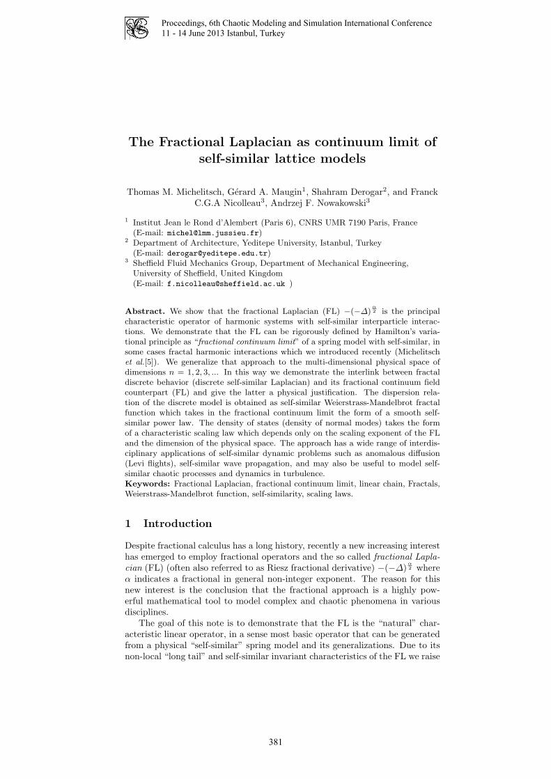
Proceedings, 6th Chaotic Modeling and Simulation International Conference
11 - 14 June 2013 Istanbul, Turkey
The Fractional Laplacian as continuum limit ofself-similar lattice models
Thomas M. Michelitsch, Gerard A. Maugin1, Shahram Derogar2, and FranckC.G.A Nicolleau3, Andrzej F. Nowakowski3
1 Institut Jean le Rond d’Alembert (Paris 6), CNRS UMR 7190 Paris, France(E-mail: [email protected])
2 Department of Architecture, Yeditepe University, Istanbul, Turkey(E-mail: [email protected])
3 Sheffield Fluid Mechanics Group, Department of Mechanical Engineering,University of Sheffield, United Kingdom(E-mail: [email protected] )
Abstract. We show that the fractional Laplacian (FL) −(−∆)α2 is the principal
characteristic operator of harmonic systems with self-similar interparticle interac-tions. We demonstrate that the FL can be rigorously defined by Hamilton’s varia-tional principle as “fractional continuum limit” of a spring model with self-similar, insome cases fractal harmonic interactions which we introduced recently (Michelitschet al.[5]). We generalize that approach to the multi-dimensional physical space ofdimensions n = 1, 2, 3, ... In this way we demonstrate the interlink between fractaldiscrete behavior (discrete self-similar Laplacian) and its fractional continuum fieldcounterpart (FL) and give the latter a physical justification. The dispersion rela-tion of the discrete model is obtained as self-similar Weierstrass-Mandelbrot fractalfunction which takes in the fractional continuum limit the form of a smooth self-similar power law. The density of states (density of normal modes) takes the formof a characteristic scaling law which depends only on the scaling exponent of the FLand the dimension of the physical space. The approach has a wide range of interdis-ciplinary applications of self-similar dynamic problems such as anomalous diffusion(Levi flights), self-similar wave propagation, and may also be useful to model self-similar chaotic processes and dynamics in turbulence.Keywords: Fractional Laplacian, fractional continuum limit, linear chain, Fractals,Weierstrass-Mandelbrot function, self-similarity, scaling laws.
1 Introduction
Despite fractional calculus has a long history, recently a new increasing interesthas emerged to employ fractional operators and the so called fractional Lapla-cian (FL) (often also referred to as Riesz fractional derivative) −(−∆)
α2 where
α indicates a fractional in general non-integer exponent. The reason for thisnew interest is the conclusion that the fractional approach is a highly pow-erful mathematical tool to model complex and chaotic phenomena in variousdisciplines.
The goal of this note is to demonstrate that the FL is the “natural” char-acteristic linear operator, in a sense most basic operator that can be generatedfrom a physical “self-similar” spring model and its generalizations. Due to itsnon-local “long tail” and self-similar invariant characteristics of the FL we raise
381

Proceedings, 6th Chaotic Modeling and Simulation International Conference
11 - 14 June 2013 Istanbul, Turkey
the question what is the interlink of the FL with fractal and chaotic featuresoften chosen in nature.
Recently many models where developed which employ the FL in variousphysical contexts, among them the description of “complex” dynamic phe-nomena including anomalous diffusion (Levi flights) [1–3,8,10] and see also thenumerous references therein.
This note is organized as follows: As point of departure we introduce a 1Dharmonic spring model with harmonic elastic potential energy which describesself-similar interparticle interactions which we developed recently [5]. Thisdiscrete model leads to fractal dynamic vibrational characteristics such as adispersion relation of the form of Weierstrass-Mandelbrot fractal functions.Application of Hamilton’s variational principle defines a discrete self-similarLaplacian with all good properties of a Laplacian: The self-similar Laplacianis self-adjoint, elliptic, negative (semi-) definite (indicating elastic stability),and translational invariant. We introduce a fractional continuum limit whichyields in rigorous manner the FL. In this way the FL is physically justifiedbeing a continuum description of a self-similar spring model. The approach isgeneralized to n dimensions of the physical space.
2 Linear chain model with self-similar harmonicinteractions
We consider an infinite sequence of points hp generated by a non-linear map-ping with (initial value h = h0)
hp+1 = N(hp) = Np(h), hp+1 = N−1(hp) = N−p(h) (1)
where we exclude for convenience periodic orbits and fixed points. All pointsof the sequence are assumed to fulfil hp = hq for p = q (−∞ < p < ∞). Definea function Φ for a arbitrary generated by the series
Φ(h) =
∞∑s=−∞
a−δsf(hs) (2)
where the sum is performed over the infinite sequence of points hs of (1). Φ(h)is defined (convergent) for sufficiently good functions f . Function Φ behavesself-similar under the (in general non-linear) transformation h → N(h) of itsargument, namely
Φ(N(h)) = aδ∞∑
s=−∞a−δ(s+1)f(hs+1) = aδΦ(h) (3)
For the sake of simplicity but without loss of generality let us consider here asequence generated by a linear mapping
N(h) = ah, a > 1 (4)
382

Proceedings, 6th Chaotic Modeling and Simulation International Conference
11 - 14 June 2013 Istanbul, Turkey
Then we introduce the self-similar elastic potential in the form of a self-similarfunction (3), namely
W(x, h) =1
4
∞∑s=−∞
a−δs(u(x+ has)− u(x))2 + (u(x− has)− u(x))2
(5)
which is self-similar in the sense of (3) with respect to h. The elastic potentialdescribes a homogeneous mass distribution where each material point x is con-nected with other material points x±has by a self-similar distribution of linearsprings of spring constants ∼ a−δs. In general this potential can be definedalso for nonlinear sequence hs of (1). The notion of self-similarity at a pointwas coined by Peitgen et al.[9].
The total elastic energy of (5) is given by
V (h) =
∫ ∞
−∞W(x, h) dx (6)
A self-similar Laplacian is then defined by Hamilton’s principle
∆δ,hu(x) = − δV
δu(x)(7)
where δ(..)δu stands for a functional derivative, and where
∆(δ,a,h)u(x) =∞∑
s=−∞a−δs (u(x+ has) + u(x− has)− 2u(x)) , 0 < δ < 2
(8)fulfilling self-similarity condition ∆δ,ah = aδ∆δ,h. This Laplacian has all re-quired good properties. The dispersion relation (negative eigenvalues) of thisLaplacian are obtained in the form of Weierstrass-Mandelbrot functions
ω2(δ,a)(kh) = 4
∞∑s=−∞
a−δs sin2 (khas
2), 0 < δ < 2 (9)
which are self-similar ω2(δ,a)(kah) = aδω2
(δ,a)(kh) within its entire interval of
existence 0 < δ < 2. The dispersion relation (9) is within 0 < δ < 1 a nowheredifferentiable fractal function of estimated Hausdorff dimension 2 − δ [4,5].In figures 1-3 cases of increasing fractal dimension (decreasing δ) are plotted.Note that for 1 ≤ δ < 2 (9) is a non-fractal function of Hausdorff dimensionD = 1 (see figure 1). For increasing fractal dimension D (decreasing exponentδ) fractal dispersion curves have increasingly erratic characteristics. For moredetails we refer to our paper Michelitsch et al.[5].
383

Proceedings, 6th Chaotic Modeling and Simulation International Conference
11 - 14 June 2013 Istanbul, Turkey
0 0.5 1 1.50
2
4
6
8
10
12
kh
ω2 (k
h)
δ=1.2 (nonfractal case D=1)
Fig. 1. Dispersion relation (9) for a non-fractal case.
0 0.5 1 1.50
2
4
6
8
10
12
14
kh
ω2 (k
h)
D=1.3
Fig. 2. Dispersion relation (9) for a non-fractal case.
0 0.5 1 1.50
10
20
30
40
50
60
70
kh
ω2 (k
h)
D=1.9
Fig. 3. Dispersion relation (9) for a fractal case.
384

Proceedings, 6th Chaotic Modeling and Simulation International Conference
11 - 14 June 2013 Istanbul, Turkey
3 The FL as fractional continuum limit of the discretechain Laplacian and its generalization to n dimensions
Now we define the fractional continuum limit as follows [6,7]
Λa(h) = lima→1
∞∑s=−∞
a−δsf(ash) ≈ hδ
ζ
∫ ∞
0
f(τ)
τ δ+1dτ (10)
where a = 1 + ζ → 1 and 0 < ζ << 1. The fractional continuum limit of theelastic potential (5) takes then the form
W(x, h) ≈ hδ
4ζ
∫ ∞
0
(u(x+ τ)− u(x))2 + (u(x− τ)− u(x))2
τ δ+1dτ, 0 < δ < 2
(11)which can be generalized to n dimensions as
W(x, h, α) ≈ hα
4ζ
∫ ∞
0
(u(x+ r)− u(x))2 + (u(x− r)− u(x))2
τα+ndnr (12)
where 0 < α < 2. Hamilton’s principle yields from (12) the fractional contin-uum limit of the self-similar Laplacian in n dimensions
∆n,α,hu(x) =: − δV
δu(x)=
hα
2ζ
∫ ∞
0
(u(x+ r) + u(x− r)− 2u(x))
τα+ndnr (13)
with 0 < α < 2. (13) recovers for n = 1 also the fractional continuumlimit of the self-similar Laplacian (8). The dispersion relation is obtained by∆n,α,he
ikx = −ω2n,α,h(kh)e
ikx and yields [8] a power-law of the form
ω2n,α,h(kh) = An,αk
α, 0 < α < 2 (14)
with the positive constant [8]
An,α =hα
ζ
πn2
2α−1α
Γ (1− α2 )
Γ (α+n2 )
> 0, 0 < α < 2 (15)
The positiveness of this constant is a consequence of the elastic stability.The following observation is crucial: The fractional continuum limit Lapla-
cian (13) coincides (up to a normalization factor) with the FL which is defined,e.g. [2,3,10]
∆n,α,h = −An,α (−∆)α2 (16)
where the constant (15) is consistent with the normalization factor given by inthe literature e.g. [2,3,10] and where (13) recovers with (16) and (15) the stan-dard representation of the FL. Our self-similar chain model represents hencea discrete lattice counterpart which corresponds in the fractional continuumapproximation the FL fractional approach.
385

Proceedings, 6th Chaotic Modeling and Simulation International Conference
11 - 14 June 2013 Istanbul, Turkey
With (15) it is straight-forward to obtain the density of normal modes(“density of states”) D(ω) where D(ω)dω measures the number of eigenmodesof frequency ω. It is obtained as [8]
Dα,n(ω) = Bn,αω2nα −1, 0 < α < 2 (17)
with
Bn,α =22−n
πn2 Γ (n2 )αA
nαn,α
(18)
We observe that the state density Dα,n(ω) scales as ∼ ω2nα −1 with a positive
exponent where 0 < n − 1 < 2nα − 1 depending only on physical dimension n
and α. Because of 0 < α < 2 the scaling exponent of the self-similar density ofstates (17) is always greater than the exponent n−1 of the standard Laplacianwhich is asymptotically approached by (17) when α approaches the forbiddenvalue α → 2.
4 Conclusions
We have demonstrated in this brief note that the fractional Laplacian can berigorously defined as the fractional continuum limit by a self-similar linearspring model and its generalization to n = 1, 2, 3.. dimensions. In this way aphysical justification for the FL is introduced. The model also reveals the in-terlink between fractal vibrational Weierstrass-Mandelbrot characteristics andits smooth fractional continuum counterpart. The present approach allows todevelop a smooth fractional field theory of phenomena with fractal and erratic- chaotic features [8]. Especially noteworthy is a vast potential of applicationswhich include dynamic processes such as anomalous diffusion (Levi flights),wave propagation and turbulence problems.
References
1.D. Brockmann and L. Hufnagel, Front Propagation in Reaction-Superdiffusion Dy-namics: Taming Levy Flights with Fluctuations, Phys. Rev. Lett. 98, 178301(2007.
2.Z.-Q. Chen, P. Kim, R. Song, Heat kernel estimates for the Dirichlet FL, J. Eur.Math. Soc. 12, 1307-1329 (2008).
3.A. Hanyga, Multi’dimensional solutions of space-time fractional diffusion equations,Proc. R. Soc. Lond. A, 458, 429-450 (2002). doi: 10.1098/rspa.2001.0893
4.G.H. Hardy, Weierstrass’s non-differentiable function. In: Trans. Amer. Math. Soc..Bd. 17, Nr. 3, 1916, S. 301-325, doi:10.1090/S0002-9947-1916-1501044-1.
5.T.M. Michelitsch, G.A. Maugin, F. C. G. A. Nicolleau, A. F. Nowakowski, S.Derogar. Dispersion relations and wave operators in self-similar quasicontinuouslinear chains. Physical Review E 80, 011135, 2009.
6.T. M. Michelitsch, The self-similar field and its application to a diffusion problem,J. Phys. A: Math. Theor. 44 465206, 2011.
386

Proceedings, 6th Chaotic Modeling and Simulation International Conference
11 - 14 June 2013 Istanbul, Turkey
7.T.M. Michelitsch, G.A. Maugin, M. Rahman, S. Derogar, A.F. Nowakowski, F. C.G. A. Nicolleau, A continuum theory for one-dimensional self-similar elasticityand applications to wave propagation and diffusion, European Journal of AppliedMathematics, vol. 23, pp. 709-735, 2012).
8.T.M. Michelitsch, G.A. Maugin, A.F. Nowakowski, F. Nicolleau, The fractionalLaplacian as a limiting case of a self-similar spring model and applications ton-dimensional anomalous diffusion. Fractional Calculus and Applied Analysis, inpress.
9.H.O. Peitgen, H. Juergens, D. Saupe, Fractals for the Classroom” Part Two,Springer-Verlag, New York, und NCTM, 1992.
10.J. L. Vazquez (2010), Nonlinear Diffusion with Fractional Laplacian Operators.In Nonlinear partial differential equations: the Abel Symposium 2010; Holden,Helge & Karlsen, Kenneth H. eds., Springer, 2012. Pp. 271-298.
387

Proceedings, 6th Chaotic Modeling and Simulation International Conference
11 - 14 June 2013 Istanbul, Turkey
388

Proceedings, 6th Chaotic Modeling and Simulation International Conference
11 - 14 June 2013 Istanbul, Turkey
Laceability in the Brick Product of Cycles
Dr. R.Murali
*, Shivaputra
#, Chetan.S
#
*Department of Mathematics, Dr.Ambedkar Institute of Technology, India.
#Department of Electronics and Communication Engineering, Dr. Ambedkar
Institute of Technology, India
E-mail: [email protected]
Abstract: B. Alspach, C.C. Chen and Kevin Mc Avaney [1] have discussed the
Hamiltonian laceability of the Brick product C(2n, m, r) for even cycles. In [2], the
authors have explored the Hamiltonian laceability properties of (m,r)-Brick Product
C(2n+1, 1, r) for r=2,3. In [3] the authors have established Hamiltonian laceability
properties of C(2n+1, 1, r) for r=3,4. In this paper we present the Hamiltonian
laceability properties of C(2n+1, 1, r) for r=5,6,and 7.
Keywords - Brick product, Connected graph, Hamiltonian-t-laceable graph. 2000 Mathematics subject classification: 05C45, 05C99
.
1. INTRODUCTION
Let G be a finite, simple, connected and undirected graph. Let u
and v be two vertices in G. The distance between u and v in G,
denoted by d(u,v) is the length of a shortest u-v path in G. G is
Hamiltonian laceable if there exists in G a Hamiltonian path
between every pair of distinct vertices in G at an odd distance. G is
Hamiltonian-t-laceable (Hamiltonian-t*-laceable) if there exists a
Hamiltonian path between every pair of distinct vertices (at least
one pair of distinct vertices) u and v in G with the property
d(u,v)=t , 1 ≤ t ≤ diamG. Hamiltonian laceability in the Brick
product of even cycles was studied by B.Alspach, C.C.Chen and
Kevin McAvaney in [1]. In [2] and [3], the authors have discussed
the Hamiltonian laceability properties of the (m,r)-Brick Product
of odd cycles C(2n+1,m,r) for r=2,3 and 4. In this paper we
explore the Hamiltonian-t-laceability of the (m,r)-Brick Product
C(2n+1,1,r) for r=5,6 and 7.
Definition 1: (Brick Product of even cycles):
Let m, n and r be a positive integers. Let C2n- a0,a1,a2,a3…..a(2n-1)a0
denote a cycle of order 2n. The (m,r)-brick product of C2n denoted
389

Proceedings, 6th Chaotic Modeling and Simulation International Conference
11 - 14 June 2013 Istanbul, Turkey
by C(2n,m,r) is defined as follows. For m=1, we require that r be
odd and greater than 1. Then, C(2n,m,r) is obtained from C2n by
adding chords a2k(a2k+r), k=1,2,….n, where the computation is
performed under modulo 2n.
From the definition above, it is clear that the Brick product
of even cycles is a connected three regular graph.
The following figure 1 shows the Brick product of the
cycle C10 for r = 5.
Fig. 1: Brick product C(10,1,5)
Definition 2: (Brick Product of odd cycles):
Let m,n and r be positive integers. Let C2n+1=a0 a1 a2 a3………a2n a0
denote a cycle of order 2n+1 (n>1). The (m,r)-brick product of
C2n+1, denoted by C(2n+1,m,r) is defined as follows. For m=1, we
require that 1< r < 2n. Then C(2n+1,m,r) is obtained from C2n+1 by
adding chords ak(ak+r), 0 ≤ k ≤ 2n where the computation is
performed under modulo 2n+1.
From the definition above, it is clear that the Brick product
of odd cycles is a connected four regular graph.
390

Proceedings, 6th Chaotic Modeling and Simulation International Conference
11 - 14 June 2013 Istanbul, Turkey
The following figure 2 shows the Brick product of the
cycle C13 for r=2.
Fig.2: The Brick product C (13, 1, 2)
Definition 3: Let u and v be two distinct vertices in a connected
graph G. Then u and v are attainable in G if there exists a
Hamiltonian path in G between u and v.
Terminologies used in the Brick Product to determine the
Hamiltonian path:
For m=1, if ai is any vertex of C (2n+1, m, r), then the following
are defined.
(ai) P[m] = (ai)( ai+1)( ai+2) . . . . . . . .(ai+m-1)
(ai) P-1
[m] = (ai)(ai-1)( ai-2) . . . . . . . . (ai-m+1)
(ai) [J] = (ai)( ai+r) and (ai)[J-1
] = (ai)( ai-r)
(ai) [K] = (ai)( ai+2) and (ai)[K-1
] = (ai)( ai-2)
Example: For n= 4, consider the graph C(2n+1, 1, 4). For the
vertices ai and aj in G, we have d(ai, aj) = 2 for i =1 and j =3.
Using the above notations, a Hamiltonian path in G between the
vertices a1 and a3 is given by (ai) P(2) J [P-1
(2)]2 J
-1 [P
-1(2)]
2(n-3) J
-1
= a1-a2-a6-a5-a4-a0-a8-a7-a3 under modulo 2n+1.
The following figure 3 shows the Hamiltonian path
between the vertices a1 and a3.
391
Proceedings, 6th Chaotic Modeling and Simulation International Conference
11 - 14 June 2013 Istanbul, Turkey
Fig.3: Hamiltonian path from vertex a1 to a3 in the Brick
Product C(9,1,4)
Definition 4: Let ai and aj be any two distinct vertices in a
connected graph G. Let E’ be a minimal set of edges not in G and
P be a path in G such that P E’ is a Hamiltonian path in G from
ai to aj. Then | E’| is called the t-laceability number (t) of ),( ji aa
and the edges in E’ are called the t-laceability edges with respect
to ),( ji aa .
2. RESULTS
In [2] the authors proved the following result:
Theorem 5: The graph G=C(2n+1, 1, 2) is Hamiltonian-t-
laceable for 1≤t≤diamG.
In [3] the authors proved the following results:
Theorem 6: The graph C(2n+1, 1, 3) is Hamiltonian-t-laceable
for t=1,2 if n=3 and is Hamiltonian-t-laceable for t=1,2,3 if n≥6
such that (2n+1)1(mod 3).
392

Proceedings, 6th Chaotic Modeling and Simulation International Conference
11 - 14 June 2013 Istanbul, Turkey
Theorem 7: The graph C(2n+1, 1, 3) is Hamiltonian-t-laceable
for t=1,2,3. Where n≥5 such that (2n+1) 2(mod 3).
Theorem 8: The graph C(2n+1, 1, 4) is Hamiltonian-t-laceable
for t=1,2 if n = 4 and is Hamiltonian-t-laceable for t=1,2,3 if n ≥
6 such that (2n+1) 1(mod 4).
Theorem 9: The graph C(2n+1, 1, 4) is Hamiltonian-t-laceable
for t=1,2,3. Where n ≥ 5 such that (2n+1)3(mod 4).
We now prove the following results:
Theorem 10: The graph G=C(2n+1,1,5) for n≥5 and n≠7+5k is
Hamiltonian-t-laceable for t=1. For t=2, G is Hamiltonian-t-
laceable with (t)=1, where k is a non negative integer.
Proof: Consider the graph G= C(2n+1, 1, 5).
Let d(ai, aj) = t, (0 ≤ i < j ≤ 2n). For convenience we take j>i.
Claim 1: G is Hamiltonian-t-laceable for t=1
Case (i): j - i = 1 or (2n+1)-(j-i) =1
If j - i = 1 or (2n+1)-(j-i) =1 in C2n+1 then, ai and aj are attainable in
G, since (ai) [P-1
(2)]2n
is the Hamiltonian path.
393

Proceedings, 6th Chaotic Modeling and Simulation International Conference
11 - 14 June 2013 Istanbul, Turkey
Fig.4: Hamiltonian path from vertex a0 to a1 in the Brick
Product C(13,1,5)
Case (ii): j - i = 5 or (2n+1)-( j - i) =5
If j - i = 5 in C2n+1 then, ai and aj are attainable in G, since
(ai) [P(2)]4 J
-1[(P
-1(2)]
2n-5 is the Hamiltonian path.
If (2n+1)-( j - i) =5 in C2n+1 then, ai and aj are attainable in G, since
(ai) [P-1
(2)]4 J [P(2)]
2n-5 is the Hamiltonian path.
Claim 2: G is Hamiltonian-t-laceable for t=2
Case(i): j - i = 2 or (2n+1)-( j - i) =2
If j - i = 2 or (2n+1)-( j - i) =2 in C2n+1 then, ai and aj are attainable
in G, since (ai) P(2) K-1
[P-1
(2)]2(n-1)
is a Hamiltonian path with t-
laceability edge K-1
.
Case(ii): j - i = 6 or (2n+1)-( j - i) = 6
If j - i = 6 or (2n+1)-( j - i) = 6 in C2n+1 then, ai and aj are attainable
in G, since (ai) J [P-1
(2)]4
K-1
[P-1
(2)]n+5
is the Hamiltonian path
with t-laceability edge K-1
.
Case(iii): If j - i = 4 or (2n+1)-( j - i) =4
If j - i = 4 or (2n+1)-( j - i) =4 in C2n+1 then, ai and aj are attainable
in G, since (ai) J [P(2)]n+6
K [P(2)]8 is the Hamiltonian path with t-
laceability edge K.
394

Proceedings, 6th Chaotic Modeling and Simulation International Conference
11 - 14 June 2013 Istanbul, Turkey
Hence the proof.
Theorem 11: The graph G=C(2n+1,1,6) for n ≥ 6 and n ≠7+3k
is Hamiltonian-t-laceable for t=1. For t=2, G is Hamiltonian-t-
laceable with (t)=1, where k is a non negative integer.
Proof: Consider the graph G= C(2n+1, 1, 6).
Let d(ai, aj) = t, (0 ≤ i < j ≤ 2n). For convenience we take j>i.
Claim 1: G is Hamiltonian-t-laceable for t=1
Case (i): j - i = 1 or (2n+1)-(j-i) =1
If j - i = 1 or (2n+1)-(j-i) =1 in C2n+1 then, ai and aj are attainable in
G, since (ai) [P-1
(2)]2n
is the Hamiltonian path.
Case (ii): j - i = 6 or (2n+1)-( j - i) =6
If j - i = 6 in C2n+1 then, ai and aj are attainable in G, since
(ai) [P(2)]5 J
-1[(P
-1(2)]
2n-6 is the Hamiltonian path.
If (2n+1)-( j - i) = 6 in C2n+1 then, ai and aj are attainable in G,
since (ai) [P-1
(2)]5 J [P(2)]
2n-6 is the Hamiltonian path.
Claim 2: G is Hamiltonian-t-laceable for t=2
If n=6 then (ai) J [P(2)]6 K [P(2)]
5 is a Hamiltonian path with t-
laceability edge K. If n ≥ 7 then
Case(i): j - i = 2 or (2n+1)-( j - i) =2
If j - i = 2 or (2n+1)-( j - i) =2 in C2n+1 then, ai and aj are attainable
in G, since (ai) P(2) K-1
[P-1
(2)]2(n-1)
is a Hamiltonian path with t-
laceability edge K-1
.
Case(ii): j - i = 5 or (2n+1)-( j - i) = 5
If j - i = 5 or (2n+1)-( j - i) = 5 in C2n+1 then, ai and aj are attainable
in G, since (ai) J [P-1
(2)]n-7
K-1
[P-1
(2)]n+5
is the Hamiltonian path
with t-laceability edge K-1
.
Case(iii): If j - i = 7 or (2n+1)-( j - i) =7
If j - i = 7 or (2n+1)-( j - i) =7 in C2n+1 then, ai and aj are attainable
in G, since (ai) J [P-1
(2)]2(n-3)
K [P-1
(2)]n-8
is the Hamiltonian path
with t-laceability edge K.
395

Proceedings, 6th Chaotic Modeling and Simulation International Conference
11 - 14 June 2013 Istanbul, Turkey
Hence the proof.
Theorem 12: The graph C(2n+1,1,7) is Hamiltonian-t-laceable
for t=1 if n ≥ 7 and n ≠10+7k where k is a non negative integer.
Proof: Consider the graph G= C(2n+1, 1, 7).
Let d(ai, aj) = t, (0 ≤ i < j ≤ 2n). For convenience we take j>i.
Case (i): j - i = 1 or (2n+1)-(j-i) =1
If j - i = 1 or (2n+1)-(j-i) =1 in C2n+1 then, ai and aj are attainable in
G, since (ai) [P-1
(2)]2n
is the Hamiltonian path.
Fig.5: Hamiltonian path from vertex a0 to a1 in the Brick
Product C(19,1,7)
Case (ii): j - i = 7 or (2n+1)-( j - i) =7
If j - i = 7 in C2n+1 then, ai and aj are attainable in G, since
(ai) [P(2)]6 J
-1[(P
-1(2)]
2n-7 is the Hamiltonian path.
If (2n+1)-( j - i) = 7 in C2n+1 then, ai and aj are attainable in G,
since (ai) [P-1
(2)]6 J [P(2)]
2n-7 is the Hamiltonian path.
Hence there exists Hamiltonian path between an every pair of
vertices in G such that d(ai,aj)=1. Therefore G is Hamiltonian-t-
laceable for t=1.
Hence the proof.
396

Proceedings, 6th Chaotic Modeling and Simulation International Conference
11 - 14 June 2013 Istanbul, Turkey
3. REFERENCES:
[1] Brain Alspach, C.C. Chen and Kevin McAvaney, On a class of
Hamiltonian laceable 3-regular graphs, Discrete Mathematics,
151(1996), pp. 19-38
[2] Leena N. shenoy and R.Murali, Laceability on a class of
Regular Graphs, International Journal of computational
Science and Mathematics, volume 2, Number 3 (2010), pp.
397-406.
[3] Girisha.A, H.Mariswamy, R.Murali and G.Rajendra,
Hamiltonian Laceability in a class of 4-Regular Graphs, IOSR
Journal of Mathematics, Volume 4, Issue 1 (Nov. - Dec. 2012),
pp. 07-12.
[4] Girisha.A and R.Murali, Hamiltonian Laceability in cyclic
product and brick product of cycles, International Journal of
Graph Theory, Volume 1, Issue 1, February 2013, pp. 32-40.
[5] F. Harary, Graph Theory, Narosa Publishing House, Reprint,
1990.
*************
397

Proceedings, 6th Chaotic Modeling and Simulation International Conference
11 - 14 June 2013 Istanbul, Turkey
398

Proceedings, 6th Chaotic Modeling and Simulation International Conference
11 - 14 June 2013 Istanbul, Turkey
Some aspects of stochastic calculus
and approximation in chaoticsystems analysis
Gabriel V. Orman and Irinel Radomir
Department of Mathematics and Computer Science”Transilvania” University of Brasov, 500091 Brasov, Romania.
E-mail: [email protected]
Abstract. Frequently when we refer to chaos and chaotic and complexsystems to describe the comportment of some natural phenomena, in factwe consider phenomena of the type of a Brownian motion which is a morerealistic model of such phenomena. Thus one can talk about a passing fromchaotic and complex systems to Brownian motion. Some aspects regardindthe Brownian motion and its Markovian nature will be developed, in short, inthis paper; we try also to emphasize their impact for some practical problems.
Keywords: stochastic differential equations, stochastic calculus, Markovprocesses, Brownian motion.
1 Introduction
It is known that a chaotic perpetual motion of a Brownian particle is theresult of the collisions of particle with the molecules of the fluid in whichthere is.
But this particle is much bigger and also heavier than the molecules of thefluid which it collide, and then each collision has a negligible effect, while thesuperposition of many small interactions will produce an observable effect.
On the other hand, for a Brownian particle such molecular collisions ap-pear in a very rapid succession, their number being enormous. For a so highfrequency, evidently, the small changes in the particle’s path, caused by eachsingle impact, are too fine to be observable. For this reason the exact pathof the particle can be described only by statistical methods.
We emphasize that L. Bachelier derived the law governing the position of asingle grain performing a 1-dimensional Brownian motion starting at a ∈ Rat time t = 0; and A. Einstein also derived the same law from statisticalmechanical considerations and applied it to the determination of moleculardiameters.
399

Proceedings, 6th Chaotic Modeling and Simulation International Conference
11 - 14 June 2013 Istanbul, Turkey
Also Paul Levy found a construction of the Brownian motion and givena profound description of the fine structure of the individual Brownian path.D. Ray obtained some results in the case when the motion is strict Markov;and W. Feller obtained that the generator of a strict Markovian motion withcontinuous paths (diffusion) can be expressed as a differential operator.
And in the last time we can speak about Markov processes from KiyosiIto’s perspective (according to D.W. Stroock). The usual class of Markovprocesses which we consider has many times some restrictions which do notcover many interesting processes. This is the reason for which we try oftento obtain some extensions of this notion.
Researches in this direction are due especially to K. Ito and in this contextwe shall refer below, in short, to some of them.
2 On Markov processes - an extended defini-
tion
Let S be a state space and consider a particle which moves in S. Also, supposethat the particle starting at x at the present moment will move into the setA ⊂ S with probability pt(x,A) after t units of time, “irrespectively of itspast motion”, that is to say, this motion is considered to have a Markoviancharacter.
The transition probabilities of this motion are pt(x,A)t,x,A and we con-sidered that the time parameter t ∈ T = [0,+∞).
The state space S is assumed to be a compact Hausdorff space with acountable open base. The σ-field generated by the open sets (the topologicalσ-field on S) is denoted by K(S). Therefore, a Borel set A is a set in K(S)(i.e. A ∈ K(S)).
The mean valuem = M(µ) =
∫Rxµ(dx)
is used for the center and the scattering degree of a one-dimensional proba-bility measure µ having the second order moment finite, and the variance ofµ is defined by
σ2 = σ2(µ) =∫R
(x−m)2µ(dx).
On the other hand, from the Tchebychev’s inequality, for any t > 0, wehave
µ(m− tσ,m+ tσ) ≤ 1
t2,
so that several properties of 1-dimensional probability measures can be de-rived.
400

Proceedings, 6th Chaotic Modeling and Simulation International Conference
11 - 14 June 2013 Istanbul, Turkey
Remark 2.1 In the case when the considered probability measure has nofinite second order moment, σ becomes useless. In such a case one can in-troduce the central value and the dispersion that will play similar roles as mand σ for general 1-dimensional probability measures.
The dispersion δ is defined as follows
δ = δ(µ) = − log∫ ∫
R2e−|x−y|µ(dx)µ(dy).
Furthermore it is assumed that the following conditions are satisfied bythe transition probabilities pt(x,A)t∈T,x∈S,A∈K(S):
1 for t and A fixed,a) the transition probabilities are Borel measurable in x;b) pt(x,A) is a probability measure in A;
2 p0(x,A) = δx(A) (i.e. the δ-measure concentrated at x);
3 pt(x, ·)weak−→ pt(x0, ·) as x→ x0 for any t fixed, that is
limx→x0
∫f(y)pt(x, dy) =
∫f(y)pt(x0, dy)
for all continuous functions f on S;4 pt(x, U(x)) −→ 1 as t 0, for any neighborhood U(x) of x;5 the Chapman-Kolmogorov equation holds:
ps+t(x,A) =∫Spt(x, dy)ps(y, A).
We can give now the definition of a Markov process as follows:
Definition 2.1 A ”Markov process” is a system of stochastic processes
Xt(ω), t ∈ T, ω ∈ (Ω, K, Pa)a∈S,
that is for each a ∈ S, Xtt∈S is a stochastic process defined on the proba-bility space (Ω, K, Pa).
It can be observed that a definition as it is given above not correspondto many processes that are of a real interest so that it is useful to obtain anextension of this notion. An extended notion has been proposed by K. Itoand it is given below.
Let E be a separable Banach space with real coefficients and norm || · ||and let also L(E,E) be the space of all bounded linear operators E −→ E.It can be observed that L(E,E) is a linear space.
401
Proceedings, 6th Chaotic Modeling and Simulation International Conference
11 - 14 June 2013 Istanbul, Turkey
Definition 2.2 The collection of stochastic processes
X = Xt(ω) ≡ ω(t) ∈ S, t ∈ T, ω ∈ (Ω, K, Pa)a∈S
is called a ”Markov process” if the following conditions are satisfied:
1) the ”state space” S is a complete separable metric space and K(S) is atopological σ-algebra on S;
2) the ”time internal” T = [0,∞);
3) the ”space of paths” Ω is the space of all right continuous functions T −→S and K is the σ-algebra K[Xt : t ∈ T ] on Ω;
4) the probability law of the path starting at a, Pa(H), is a probability mea-sure on (Ω, K) for every a ∈ S which satisfy the following conditions:
4a) Pa(H) is K(S)-measurable in a for every H ∈ K;
4b) Pa(X0 = a) = 1;
4c) Pa(Xt1 ∈ E1, · · · , Xtn ∈ En) =∫. . .∫ai∈Ei
Pa(Xt1 ∈ da1)Pa1(Xt2−t1 ∈ da2) . . .
. . . Pan−1(Xtn−tn−1 ∈ dan) for 0 < t1 < t2 < . . . < tn.
Remark 2.2 Evidently there are some differences between this definition andDefinition 2.1 of a Markov process. Thus
i. The space S is not necessary to be compact;
ii. it is not assumed the existence of the left limits of the path;
iii. the transition operator f −→ Gtf(·) = E.(f(Xt)) do not necessarilycarry C(S) into C(S) (C(S) being the space of all real-valued boundedcontinuous functions on S).
3 The Markovian nature of the Brownian path
In his study Bachelier found some solutions of the type ψ(x). He derived1
the law governing the position of a single grain performing a 1-dimensionalBrownian motion starting at a ∈ R1 at time t = 0:
Pa[x(t) ∈ db] = g(t, a, b)db (t, a, b) ∈ (0,+∞)×R2, (1)
1Bachelier, L. Theorie de la speculation. Ann. Sci. Ecole Norm. Sup., 17, 1900, 21-86.
402
Proceedings, 6th Chaotic Modeling and Simulation International Conference
11 - 14 June 2013 Istanbul, Turkey
where g is the source (Green) function
g(t, a, b) =e−
(b−a)2
2t
√2πt
(2)
of the problem of heat flow:
∂u
∂t=
1
2
∂2u
∂a2(t > 0). (3)
Bachelier also pointed out the Markovian nature of the Brownian pathexpressed in
Pa[a1 ≤ x(t1) < b1, a2 ≤ x(t2) < b2, · · · , an ≤ x(tn) < bn] =
=
b1∫a1
b2∫a2
· · ·bn∫an
g(t1, a, ξ1) g(t2 − t1, ξ1, ξ2) · · ·
· · · g(tn − tn−1, ξn−1, ξn) dξ1 dξ2 · · · dξn, 0 < t1 < t2 < · · · tn (4)
and used it to establish the law of maximum displacement
P0
[maxs≤t
x(s) ≤ b]
= 2
b∫0
e−a2
2t
√2πt
da t > 0, b ≥ 0. (5)
It is very interesting that A. Einstein, in 1905, also derived (1) fromstatistical mechanical considerations and applied it to the determination ofmolecular diameters.2
As we already emphasized, a rigorous definition and study of Brownianmotion requires measure theory. Consider the space of continuous pathw : t ∈ [0,+∞)→ R with coordinates x(t) = w(t) and let B be the smallestBorel algebra of subsets B of this path space which includes all the simpleevents B = (w : a ≤ x(t) < b), (t ≥ 0, a < b). Wiener established theexistence of nonnegative Borel measures Pa(B), (a ∈ R, B ∈ B) for which(4) holds3. Among other things, this result attaches a precise meaning toBachelier’s statement that the Brownian path is continuous.
Paul Levy found another construction of the Brownian motion and givesa profound description of the fine structure of the individual Brownian path.
The standard Brownian motion can be now defined.
2see: A. Einstein, Investigations on the theory of the Brownian movement, New York,1956.
3N. Wiener, Differential space, Math. Phys. 2, 1923, pp. 131-174
403

Proceedings, 6th Chaotic Modeling and Simulation International Conference
11 - 14 June 2013 Istanbul, Turkey
Definition 3.1 A continuous-time stochastic process Bt | 0 ≤ t ≤ T iscalled a ”standard Brownian motion” on [0, T ) if it has the following fourproperties:
i B0 = 0.
ii The increments of Bt are independent; that is, for any finite set oftimes 0 ≤ t1 < t2 < · · · < tn < T, the random variables
Bt2 −Bt1 , Bt3 −Bt2 , · · · , Btn −Btn−1
are independent.
iii For any 0 ≤ s ≤ t < T the increment Bt−Bs has the normal distribu-tion with mean 0 and variance t− s.
iv For all ω in a set of probability one, Bt(ω) is a continuous function oft.
The Brownian motion can be represented as a random sum of integrals oforthogonal functions. Such a representation satisfies the theoretician’s needto prove the existence of a process with the four defining properties of Brow-nian motion, but it also serves more concrete demands. Especially, the seriesre-presentation can be used to derive almost all of the most important ana-lytical properties of Brownian motion. It can also give a powerful numericalmethod for generating the Brownian motion paths that are required in com-puter simulation.
Remark 3.1 Let us consider R ∪ ∞. Then one can define
pt(x, dy) =1
t√
2πe−
(y−x)2
2t2 dy in R
pt(∞, A) = δ∞A.
Let us observe that the conditions 1b) and 2-5 assumed on the transitionprobabilities pt(x,A)t∈T,x∈S,A∈K(S), given in Section 2, are satisfied in thiscase for ”Brownian transition probabilities” where R ∪ ∞ is considered asthe one-point compactification of R.
Finally we shall give an interesting result regarding to a 3-dimensionalBrownian motion.
Let X be a Markov process in a generalized sense as it is given in Def-inition 2.2. Let us denote by B(S) the space of all bounded real K(S)-measurable functions and let us consider a function f ∈ B(S).
404

Proceedings, 6th Chaotic Modeling and Simulation International Conference
11 - 14 June 2013 Istanbul, Turkey
It is supposed that
Ea
( ∞∫0
|f(Xt)|dt)
(6)
is bounded in a. Then, the following
Uf(a) = Ea
( ∞∫0
f(Xt)dt)
(7)
is well-defined and is a bounded K(S)-measurable function of a ∈ S. TheUf is called the potential of f with respect to X. Having in view thatUf = limα↓0Rαf , it is reasonable to write R0 instead of U . Based on thisfact, Rαf will be called the potential of order α of f .
It is useful to retain that Rαf ∈ B(S) for α > 0; and generally f ∈ B(S)while R0f(= Uf) ∈ B(S) under the condition (6).
Now the name potential is justified by the following theorem on the 3-dimensional Brownian motion.
Theorem 3.1 Let X be the 3-dimensional Brownian motion. If f ∈ B(S)has compact support, then f satisfies (6) and
Uf(a) =1
2π
∫R3
f(b)db
|b− a|=
1
2π×Newtonian potential of t. (8)
We do not insist on these aspects. But more details, proofs and relatedproblems can be found in [1], [2], [3], [4], [14], [6], [13], [12].
Conclusion 3.1 As we have said at the beginning, we think that when, invarious problems, we say ”chaos” or ”chaotic and complex systems” or weuse another similar expression to define the comportment of some naturalphenomena, in fact we imagine phenomena similarly to a Brownian motionwhich is a more realistic model of such phenomena. And this opinion lie atthe basis of this paper.
References
[1] A. T. Bharucha-Reid. Elements Of The Theory Of Markov Processes AndTheir Applications. Mineola, New York, 1997, Dover Publications, Inc.
[2] K. Ito, Selected Papers, Springer, 1987.
405

Proceedings, 6th Chaotic Modeling and Simulation International Conference
11 - 14 June 2013 Istanbul, Turkey
[3] K. Ito and H. P. McKean Jr. Diffusion Processes and their Sample Paths.Berlin Heidelberg, 1996, Springer-Verlag.
[4] K. Ito. Stochastic Processes. Ole E. Barndorff-Nielsen, Ken-iti Sato, edi-tors. Berlin Heidelberg, 2004, Springer-Verlag.
[5] B. Øksendal. Stochastic Differential Equations: An Introduction withApplications. Sixth Edition, New York, 2003, Springer, Berlin-Heidelberg.
[6] P. Olofsson, and M. Andersson. Probability, Statistics and StochasticProcesses, 2nd Edition. John Wiley & Sons, Inc., Publication, 2012.
[7] G. V. Orman. Lectures on Stochastic Approximation Algorithms. Theoryand Applications. Duisburg, 2001, Preprint, Univ. ”Gerhard Mercator”.
[8] G. V. Orman. Handbook Of Limit Theorems And Sochastic Approxima-tion. Brasov, 2003, Transilvania University Press.
[9] G. V. Orman. On Markov Processes: A Survey Of The Transition Prob-abilities And Markov Property. In Christos H. Skiadas and Ioannis Di-motikalis, editors, Chaotic Systems: Theory and Applications. World Sci-entific Publishing Co Pte Ltd, 2010, 224-232.
[10] G. V. Orman. On a problem of approximation of Markov chains by a so-lution of a stochastic differential equation. In Christos H. Skiadas, IoannisDimotikalis and Charilaos Skiadas, editors, Chaos Theory: Modeling, Sim-ulation and Applications. World Scientific Publishing Co Pte Ltd, 2011,30-40.
[11] G. V. Orman and I. Radomir. New Aspects in Approximation of aMarkov Chain by a Solution of a Stochastic Differential Equation. ChaoticModeling and Simulation (CMSIM) International Journal, 2012, pp. 711-718.
[12] G. V. Orman. Aspects of convergence and approximation in randomsystems analysis. LAMBERT Academic Publishing, Germany, 2012.
[13] Z. Schuss. Theory and Application of Stochastic Differential Equations.New York, 1980, John Wiley & Sons.
[14] D. W. Stroock, Markov Processes from K. Ito Perspective, PrincetonUniv. Press, Princeton, 2003.
406

Proceedings, 6th Chaotic Modeling and Simulation International Conference
11 - 14 June 2013 Istanbul, Turkey
Stabilization of an Inductorless Chua’s Chaotic
Circuit via Sliding Mode Control*
Suphaphorn Panikhom, Wirote Sangtungtong and Sarawut Sujitjorn
School of Electrical Engineering, Suranaree University of Technology,
Nakhon Ratchasima, 30000, Thailand
E-mail: [email protected]
Abstract: This article proposes stabilization of an inductorless Chua’s chaotic
circuit via sliding mode control (SMC). Modeling of the circuit and its
electronic circuit design are presented. During controller design process,
stability guarantee is required simultaneously. Since the second method of
Lyapunov’s is applied, coefficients of the Lyapunov function candidates and
their derivatives are obtained via metaheuristic search. Adaptive tabu search
(ATS) metaheuristic has been applied for the purposes, and the design is
formulated as an optimization problem with nonlinear constraints. The paper
gives details of algorithm implementation, control design, electronic circuit
design and simulation results with discussions.
Keywords:, Chua’s Circuit, Stabilization, Sliding Mode Control.
1. Introduction
Research in chaos has been a very active topic in recently years. Leon O Chua
introduced a chaotic circuit in 1983 [1] becoming a famous circuit nowadays.
The circuit is a simple and typical third-order autonomous system that exhibits
chaotic and bifurcation phenomena [2],[3]. Proper use for a chaotic system may
need its chaotic behavior during a certain period of time alternating to well-
behaved (or stabilized) dynamic. Therefore, stabilization techniques are needed
for chaotic systems. Among those in literature, it has been possible to use
traditional feedback control approach for the purpose [4]. Nonlinear feedback
control approach has been proposed with stability analysis using Hurwitz matrix
[5]. Another possibility for control and stabilization of a chaotic system is to use
backstepping method [6, 7]. Recently, sliding mode control (SMC) has been
successfully applied due to its robustness property [8-12]. The SMC forces a
system under control to be on a sliding manifold, and remain there till its
dynamic reaches an equilibrium. The method is applied to find controller
parameters with stability simultaneously guaranteed, for instance the work
reported by Wang (2009) [9]. Our proposed works employ the SMC together
with a kind of metaheuristics namely adaptive tabu search (ATS) [13]. The ATS
is an efficient intelligent search method which has been successfully applied to
*Paper included in Chaotic Systems: Theory and Applications, C.H. Skiadas and
I. Dimotikalis, Eds, World Scientific, pp 302—308, 2010.
407

Proceedings, 6th Chaotic Modeling and Simulation International Conference
11 - 14 June 2013 Istanbul, Turkey
various real-world problems [14],[15]. The simulation results from PSIM are
provided to show the effectiveness of the proposed approach.
2. Mathematic Model of Chua’s chaotic circuit
The standard form of Chua’s circuit shown in Fig.1 consists of two main parts
that are linear elements ,R L and C and a nonlinear element2
( )cg V called
Chua’s diode. The piecewise-linear (PWL) function of Chua’s diode is shown in
Fig. 2(a). The double scroll chaotic behavior in Fig. 2(b) will be occurred when
adjusting R into a suitable value.
1C 2C
R2cV
1cVLi 2( )g ci V
2( )cg VL
Fig.1 Standard unforced Chua’s circuit.
0.002
0.001
0
-0.001
-0.002
2Vc
2( )gi Vc
-4 -2 0 2 4
bG
pB aG
pB
(a) (b)
Fig.2 (a) Piecewise-linear function of the 2
( )cg V ,
(b) Phase portrait of double scroll attractor in three dimensional view.
1C2C
7R2cV
1cV
3u1u
Li2
( )g ci V
2u
Gyrator circuit
L=18mH
8R
9R
1R
6R
5R
4R
3R
2R
Chua’s Diode
3C
Fig.3 Inductorless Chua’s chaotic circuit with controller input indicated.
The modified Chua’s circuit is developed by changing the inductor to a
Gyrator circuit composed of two resistors, a capacitor and an operational
amplifier to compact the size of experimental circuit, and illuminate the noise
voltage across the inductor. Likewise, Chua’s diode can be realized by six
resistors and two operational amplifiers [2]. Furthermore, the controller inputs
-1
-0.5
0
0.5
1
-4
-2
0
2
4-3
-2
-1
0
1
2
3
initial
x1x2
x3
408

Proceedings, 6th Chaotic Modeling and Simulation International Conference
11 - 14 June 2013 Istanbul, Turkey
have been added into standard form in order to stabilize the chaotic Chua’s
circuit [3]. The schematic diagram of modified Chua’s circuit with controller
input indicated is illustrated in Fig.3.
By applying Kirchoff’s laws to the circuit, the controlled Chua’s circuit can
be represented by
1
2 1
1
2 2
1 2
1
7 1 1 1
2
3
7 2 2 2
1( )
1( )
( )1( )
c Lc c
Lc
c g cc c
dV i uV V
dt R C C C
diV u
dt L
dV i V uV V
dt R C C C
(1).
2 2 2 27( ) [ (1 2)( )(| | | |)]c b c a b c p c pf V R G V G G V B V B (2)
where 1 2,c cV V are the voltages across capacitors 1C and 2C , respectively, Li is
the current through inductor L, The nonlinearity function 2
( )cf V is an I-V
characteristic representing three segments PWL curve. The inner slopes aG , the
outer slope bG and the breakpoint voltage pB can be obtained from Fig.2(a).
Inputs 1 2,u u and 3u are sliding mode controllers.
To simplify (1) and (2), the circuit can be normalized by the following the
new notation:
1t t RC , 1 1,x Vc 2 ,Lx i 3 2x Vc
2 7 2x R x 1 7 1u R u , 3 2 7 1 3(1 )( )u C R C u
(3)
23 7( ) ( )g cf x R i V , 7 am R G ,
7 bn R G ,
Substitutes (3) into (1) and (2), so that the main bifurcation parameters of
Chua’s circuit can be obtained as 1 2C C and 2
1R C L . Normalized circuit
can be reformulated as follows
11 2 3 1
21 2
31 3 3 3
( )
( ( ))
dxx x x u
dt
dxx u
dt
dxx x f x u
dt
(4)
3 3 3 3( ) (1 2)( )(| | | |)p pf x nx m n x B x B . (5)
The schematic diagram in Fig.3 is overall an circuit of the proposed method.
The value of electronic components are selected as 1 90C nF ,
2 10C nF ,
3 0.01C µF ,1 2, 220R R ,
3 2.4R k ,4 5, 39R R k ,
6 3.3R k ,7 2R K .
8 1R ,9 1.8R M . In this case, Chua’s circuit will generate the double scroll
409
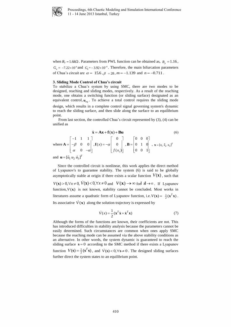
Proceedings, 6th Chaotic Modeling and Simulation International Conference
11 - 14 June 2013 Istanbul, Turkey
when 7 1.6R k . Parameters from PWL function can be obtained as, pB 1.16 ,
aG -47.22 10 and 4= 3.92 10bG . Therefore, the main bifurcation parameters
of Chua’s circuit are 15.6 , 28 , 1.139m and 0.711n .
3. Sliding Mode Control of Chua’s circuit
To stabilize a Chua’s system by using SMC, there are two modes to be
designed, reaching and sliding modes, respectively. As a result of the reaching
mode, one obtains a switching function (or sliding surface) designated as an
equivalent control, equ . To achieve a total control requires the sliding mode
design, which results in a complete control signal governing system's dynamic
to reach the sliding surface, and then slide along the surface to an equilibrium
point.
From last section, the controlled Chua’s circuit represented by (3), (4) can be
unified as
( ) x Ax f x Bu (6)
where
1 1 1
0 0
0
A ,
3
0
( ) 0
( )
x
f x
f ,
0 0 0
0 1
0 0 1
0
B , 1 2 3[ ]Tx x xx
and 1 2 3[ ]Tu u uu
Since the controlled circuit is nonlinear, this work applies the direct method
of Lyapunov's to guarantee stability. The system (6) is said to be globally
asymptotically stable at origin if there exists a scalar function ( )V x , such that
( ) 0, 0,V x x ( ) 0, 0V x x and ( )V x for x ‖ ‖ . If Lyapunov
function, ( )V x is not known, stability cannot be concluded. Most works in
literatures assume a quadratic form of Lyapunov function, i.e. ( )V x 12
( )Tx x .
Its associative ( )V x along the solution trajectory is expressed by
1
( ) ( )2
T TV x x x x x (7)
Although the forms of the functions are known, their coefficients are not. This
has introduced difficulties in stability analysis because the parameters cannot be
easily determined. Such circumstances are common when ones apply SMC
because the reaching mode can be assumed via the above stability conditions as
an alternative. In other words, the system dynamic is guaranteed to reach the
sliding surface 0s according to the SMC method if there exists a Lyapunov
function 12
( ) ( )TV s s s , and ( ) 0, 0V s s . The designed sliding surfaces
further direct the system states to an equilibrium point.
410

Proceedings, 6th Chaotic Modeling and Simulation International Conference
11 - 14 June 2013 Istanbul, Turkey
Sliding surface or switching function is a desirable scheme to force the
system dynamic to converge to an equilibrium point. A sliding surface with a
compensator inclusive is represented by
s Cx z (8)
with its dynamic described by
s = C + zx (9)
in which the compensator dynamic [12] is described by z Kx z . For a
design, the matrices C and K must be found to comply with the reaching
condition, 0s . Consequently, an equivalent control, equ , is
( )eq u CAx Cf x Kx z (10)
Replace u in (6) by equ in (10), the system under sliding mode control can be
obtained as
( ) ( ) .t x A BCA BK BC x (11)
The derivative of Lyapunov function (7) can be expressed by
1
( )2
TV x x Qx (12)
where
.T T T T T T T T Q A BCA BK BC A A C B K B C B (13)
As a necessity, on the sliding surface C and K must satisfy the following
conditions: 0 0V Q and 0s . According to such conditions, the
controlled system is asymptotically stable.
Reaching law is another necessary scheme of SMC since it governs the
system state(s) to converge to the sliding surface. One basic form of the
reaching law is constant plus proportional rate. Practically, the sgn function
generates chattering. To avoid this, one can implement a boundary layer
method, i.e. s ‖ ‖ , where represents the boundary width. This helps smooth
the switching behavior. Therefore, the reaching law can be written a
11 2( ) sq q K s s s
(14)
where 1q and 2q are positive constants, 0sK , representing total gain. The
law (14) is much simpler than that proposed by [12]. To guarantee stability, we
consider a Lyapunov function ( ) (1 2)( )TV s s s . Its derivative is obtained as
411

Proceedings, 6th Chaotic Modeling and Simulation International Conference
11 - 14 June 2013 Istanbul, Turkey
21
2( ) ( )T T
sV K s s s s s s‖ ‖ (15)
which is negative definite for 0sK . Equating (9) and (14), we obtain the
following control signal
( ) .s sK K U CAx Cf x Kx Z Cx Z (16)
From (16), one realizes that ,C K and sK must be found to satisfy
asymptotically stable conditions. This requires an efficient computing method.
Among many existing methods, metaheuristics called adaptive tabu search [13]
is our choice, and described next.
3. Search for controller parameters
ATS is chosen as a tool to find suitable controller parameters. Since the
algorithm has been known, we omit review of the ATS. Detailed explanation of
the algorithm with applications can be found in [13-15]. We apply the ATS to
search for the matrices and resulting in and , as well as a
positive constant .
An important issue of algorithm implementation is objective function.
Regarding this, the following procedures represent the objective function.
Step1. Receive parametric values of , and from ATS.
Step2. Assign parameters to the state equation in (6).
Step3. Calculate using (13) and eigenvalues of .
Step4. Based on obtained eigenvalues, determine the negative definiteness of .
If then (substitute , and in (16) by the current parameters).
- Solve the system model for the states and *.
- Calculate cost value: .
If then .
Step5. Return , , and to ATS
*Remarks: Forth-order Runge-Kutta method with is used for solving
equations. The maximum iteration is .
The ATS repeatedly search for solutions. It stops when either or
search iteration hits 1,000. Using Intel® core™ i7-2620M CPU 2.70 GHz,
RAM 8 GB, the ATS coded in MATLAB spent 7 iterations, 411.52 seconds to
reach for 0 0 0
C= 10.667 1 0
16.422 0 1
, 0 0 0
K= 10.880 17.923 17.145
3.796 -14.314 11.062
, = 1.3631 with
. The parameters C , K and sK can be substituted into U in
(2.16). This results in
C K 0Q 0V
sK
C KsK
Q Q
Q
( 0)Q C K sK
1 2,x x 3x
max max max1 2 3( ) i i if s x x x
( 0)Q 4( 10 )set f s
C K sK f s
0.01t s
max 1,000i
310f s
sK
544.53 10f s
412

Proceedings, 6th Chaotic Modeling and Simulation International Conference
11 - 14 June 2013 Istanbul, Turkey
1
2 1 2 3
3 1 2 3
0
1.141 29.953 27.812 0.363
9.0 18.76 2.108 19.848 0.726
u
u x x x
u gx x x x
(17)
4 Simulation results
Both Chua system and controllers are realized as electronics circuit. The main
electronic components are op-amps (LF351), analog multipliers (AD633), Rs
and Cs. Fig.4 shows the schematic diagram of the controlled Chua’s circuit. The
diagram is used for simulation using PSIM. The sub circuit of the obtained
controller u2 and u3 are electronically applied by using differential and
inverting amplifier circuit based on equation (17). We are interested in the states
1 2,x x and 3x . PSIM provides the results as illustrated in Fig.5. The curves
showing the states in figure 8 indicate that when the controller is switched on at
0.6t s all the states are governed to the equilibrium nicely.
R439k
R1220
R539k 220
R63.3k
R32.4k
90nC2
10nC1
R111.65k
1.8MR9
R8
1
C30.01u
L-equipvalent 18mHx2
controller3
x1
x3
igx
u3
AD633_2
10.06
1/1.65ku3
AD633_1
0.06
1
I_sensor_x2
gx3
u2
1/(1.65K*9)
controller2
x2
x1
x3
u2
I_sensor_gx3
x3x1
Chua's Diode
x1+
W
Z
x4-x3+x2-
x1+
W
Z
x4-x3+x2-
R2
G G1
G
G2
G1G2
V_sensor_x1
V_sensor_x3
Fig.4 Schematic diagram of controlled Chua’s circuit.
x3
x1 x2
0
0.5
1.0
-0.5
-1.0
0
0.002
0.004
-0.002
-0.004
0
2
4
-2
-4
0.06 0.080.02 0.04 1
0.06 0.080.02 0.04 1 0.06 0.080.02 0.04 1
Fig.5 Time response of states (a) 1,x (b) 2x and (c) 3x in PSIM.
5. Conclusion
Successful stabilization for a chaotic Chua’s circuit has been presented by this
article. The effective control utilizes sliding mode method. The article proposes
simple reaching law which can completely avoid chattering has been proposed.
To obtain controller parameters with stability guaranteed simultaneously
requires complicated computing. Regarding this, the ATS has been applied to
413

Proceedings, 6th Chaotic Modeling and Simulation International Conference
11 - 14 June 2013 Istanbul, Turkey
search for the controller parameters as well as ( )V x and ( )V x simultaneously.
The theoretical approach has been tested using electronic circuit
implementation. Simulation results agree very well indicating successful
stabilization without drawing excessive control signals.
Acknowledgement
The authors gratefully acknowledge the financial supports by Rajamangala
University of Technology Isarn, Suranaree University of Technology, and the
Office of the Higher Education Commission under NRU Project of Thailand.
References
1. T. Matsumoto, A chaotic from Chua’s circuit, IEEE Trans. Circuits Syst, vol. CAS-31,
no. 12, 1055-1058, 1984.
2. K. S. Tang, K. F. Man, G. Q. Zhong, and G. Chen, Some New Circuit Design for
Chaos Generation, in G. Chen and T. Ueta (Eds.) Chaos in Circuits and Systems,
World Scientific, Singapore, 2002, 171–190.
3. L. A. B. Tôrres, L. A. Aguirre, R. M. Palhares, and E. M. A. M. Mendes, Chaos
Control for Chua's Circuits. Control Of Chaos In Nonlinear Circuits And Systems:
97-164. 2008.
4. G. Chen and X. Dong, On feedback control of chaotic continuous-time systems,
Circuits and Systems I: Fundamental Theory and Applications, IEEE Transactions
on, vol. 40, 591-601, 1993.
5. M. Chen and Z. Han, Controlling and synchronizing chaotic Genesio system via
nonlinear feedback control, Chaos, Solitons & Fractals, vol. 17, 709-716, 2003.
6. J. Lü and S. Zhang, Controlling Chen's chaotic attractor using backstepping design
based on parameters identification, Physics Letters A, vol. 286, 148-152, 2001.
7. M. T. Yassen, Chaos control of chaotic dynamical systems using backstepping design,
Chaos, Solitons & Fractals, vol. 27, 537-548, 2006.
8. J. Y. Hung, W. Gao, and J. C. Hung, Variable structure control: a survey, Industrial
Electronics, IEEE Transactions on, vol. 40, 2-22, 1993.
9. G. Weibing and J. C. Hung, Variable structure control of nonlinear systems: a new
approach, Industrial Electronics, IEEE Transactions on, vol. 40, 45-55, 1993.
10. T.-Y. Chiang, M.-L. Hung, J.-J. Yan, Y.-S. Yang, and J.-F. Chang, Sliding mode
control for uncertain unified chaotic systems with input nonlinearity, Chaos,
Solitons & Fractals, vol. 34, 437-442, 2007.
11. J. M. Nazzal and A. N. Natsheh, Chaos control using sliding-mode theory, Chaos,
Solitons & Fractals, vol. 33, 695-702, 2007.
12. H. Wang, Z. Han, Q. Xie, and W. Zhang, Sliding mode control for chaotic systems
based on LMI, Communications in Nonlinear Science and Numerical Simulation,
vol. 14, 1410-1417, 2009.
13. D. Puangdownreong, S. Sujitjorn, and T. Kulworawanichpong, Convergence
Analysis of Adaptive Tabu Search, ScienceAsia, vol. 30, 183-190, 2004.
14. D. Puangdownreong, K. N. Areerak, A. Srikaew, S. Sujitjorn, and P. Totarong,
"System identification via Adaptive Tabu Search," In Proc. IEEE Int. Conf. on
Industrial Technology (ICIT’02), Bangkok, Thailand, vol. 2, 915-920,2002.
15. T. Kulworawanichpong, K-L. Areerak, K-N. Areerak, and S. Sujitjorn, Harmonic
Identification for Active Power Filters Via Adaptive Tabu Search Method, Lecture
Notes in Computer Science, Springer-Verlag Heidelberg, 2004, 687-694.
414

Proceedings, 6th Chaotic Modeling and Simulation International Conference
11 - 14 June 2013 Istanbul, Turkey
Self-organization in the thin gas-sensitiveAg-containing polyacrylonitrile films
V. Petrov, N. Plugotarenko, T. Semenistaya
Southern Federal University, Rostov-on-Don, RussiaE-mail: [email protected]
Abstract: The surface of thin gas-sensitive Ag-containing polyacrylonitrile films isinvestigated by a method of atomic force microscopy. The assumption of existence in thestudied spatial distributed system of signs of the determined chaos is confirmed withcalculation of parameters of nonlinear dynamics. The interrelation between extent of self-organization in films of polyacrylonitrile and their gas-sensitive properties is found.Keywords: electroconductive organic polymers, gas-sensitive materials, self-organization, theory of information, atomic force microscopy.
1. IntroductionNanocomposite films of metallcontaining polyacrylonitrile (PAN), representingan organic matrix, which structure and properties change at influence of varioustemperatures, and the particles of a modifying additive dispersed in it, are aperspective material for microelectronics [1]. Ag-containing PAN filmsfabricated by pyrolysis method under the influence of incoherent IR-radiationfrom film-forming solutions, undergo transition from a liquid state of substanceto the solid-state – this stage is process of self-organization of a material. Thestructure of the disorder material is formed in nonequilibrium conditions, thesubstance when hardening changes the properties in time and is distributed non-uniformly in space, and thus in the disorder environment occurs a spatialordered structure [2]. Methods of nonlinear dynamics and theory of informationare applied to the analysis of processes of self-organization in structure ofmaterials: surface structure research of materials with various structuralorganization and revealing long-range correlations in these structures [3]. It ispossible to investigate dynamics of system, measuring any of dynamic variablesin one point at regular intervals. Thus the look and dimension of an attractor,number of degrees of freedom, correlation and fractal dimensions of a surface,Lyapunov exponents, average mutual information and other parameters ofdynamics are defined. These methods which have been originally developed forresearch of behavior of systems, changing the condition in time, are adapted forstudying of the spatial distributed systems what surfaces of the materials are.
2. Results and discussionFor carrying out researches a set of samples of Ag-containing PAN films usingdifferent technological regimes was fabricated.Sensitivity of the films was evaluated using factor of gas-sensitivity S, which iscalculated as:
415

Proceedings, 6th Chaotic Modeling and Simulation International Conference
11 - 14 June 2013 Istanbul, Turkey
S = (Rо – Rg)/Rо, Rо > Rg,
where Ro – value of resistance of a film on air, Rg – value of resistance of a filmin the atmosphere of detected gas.In view of the material surface is a fractal object general idea of fractal objectsis used for its analysis [4].Well-known in the theory of nonlinear systems Takens method is used toresearch the dynamics of formation of solid phase of gas-sensitive material ofPAN films [2]. Patterns of self-organization processes at the formation ofdisordered materials, which the PAN films are, can be studied by means of thestudy of their surface, because their surface is a "snapshot" processes ofsolidification. Proceeding from this, the fractal dimension Df of Ag-containingPAN films on the profile surface obtained with scanning probe microscopeSolver P47 Pro (NT-MDT) in tapping mode on the air in the size of areas 5×5mkm2 was measured. Step of scanning determined the choice of the lineardimensions of the scanning area and used a number of steps. Surface scancarried out with a fixed number of points N = 256 × 256 regardless of thescanned area. Distribution function of the altitude profile of the surface ρ = f(h)of studied film, begins on some level h, taken as a zero. Using Image Analysispackage processed 65536 points in a surface image of each sample forconstructing this feature. This number of points is sufficient to identify thetopology of attractor [2]. As a result of measurement of height profile for thesamples, which were carried out along the surface through discrete intervals, geta three-dimensional image of the square surface. In the course of the processingof three-dimensional images of square surface areas by using the ImageAnalysis program received a graph of the distribution function of the heightprofile. For data processing Grassbergera-Prokaččia algorithm was used [2].The first Lyapunov exponent lr was calculated using Wolf’s algorithm [5].Lyapunov exponents are topological invariants that characterize the spatio-temporal evolution and stability of the system: dynamics of formation of solid-state is determined by the spatial-temporal chaos of a small dimension.Calculation of the average mutual information I (AMI) was carried out bymethods of the theory of information, described in [3]. AMI is the maincharacteristic of the correlations in nonlinear systems. AMI invariant relative tothe different technologies and allows you to evaluate the impact of differenttechnological factors on the structure of the material.Studies have shown that application of different temperature and time regimes atforming the polymer nanocomposite films and modifying its transition metalwith different percentage concentration lead to significant changes in themorphology of its surface.Fig. 1 presents the image, obtained by AFM measurements of the surfacemorphology of a sample of Ag-containing PAN film. The distribution functionof height profile h (ρ is the density of probability) (Fig.2) and the dependence ofthe correlation dimension D = f(log2r) (Fig. 3) are given too.
416

Proceedings, 6th Chaotic Modeling and Simulation International Conference
11 - 14 June 2013 Istanbul, Turkey
Fig. 1. AFM-image of the surface morphology of Ag-containing PAN film
Fig. 2. Distribution function of height profile of Ag-containing PAN film
of
Fig. 3. Dependence D = f(log2r) of Ag-containing PAN film
Dependence of correlation dimension D = f(log2r) allows to testify the presenceor absence of self-organizing structures in nanocomposite materials PAN/Ag.The analysis showed the presence of deterministic chaos in the system. It is
417

Proceedings, 6th Chaotic Modeling and Simulation International Conference
11 - 14 June 2013 Istanbul, Turkey
noted that the surface of the films with the best gas-sensing properties formedby three levels of self-similar structures.Studies of the samples revealed that AMI has rather big range in values. AMIincreases with increase of height of surface profile of films. Samples withdisordered structure represent hundredths of units in AMI values thatcorrespond to theoretical calculations for the amorphous material. Sufficientlyhigh AMI values are observed in the samples with small value of the height ofthe surface profile (up to 30 nm) and good gas sensitivity (S = 0,46 ÷ 0,53).High AMI values prove presence of long-range correlations in the system,which may be evidence of order as a result of self-organization processes [3].Dependence of factor of gas-sensitivity on chlorine (107 ppm) and AMI valuefrom silver content by weight in PAN films fabricated at the same technologicalregimes, is resulted on fig. 4. Character of the received dependences is similar.The maximal AMI value corresponds the maximal value of factor of gas-sensitivity.Thus, the calculation of AMI allows to reveal correlations in disorderedmaterials, which conclude a certain interrelation of electrophysical and gas-sensing properties of PAN/Ag films with its morphology of the surface.
Fig. 4. Dependence of factor of gas-sensitivity (S) and AMI values (I) fromsilver content by weight in PAN films
For investigated samples Lyapunov first spatial exponent λr which haveappeared positive have been calculated. It means, that distribution of substancein space differs from equilibrium. The analysis of Lyapunov exponent testifies,that stability of structure of a material depends on technological parameters ofits formation: higher values of temperature of second stage of IR-annealing tendto increase Lyapunov exponent. It is necessary to note absence of correlationbetween values of spatial Lyapunov exponent and percentage concentration ofthe modifying additive in samples.
418

Proceedings, 6th Chaotic Modeling and Simulation International Conference
11 - 14 June 2013 Istanbul, Turkey
3. ConclusionsThe structure of the disorder materials is formed in strongly non-equilibriumconditions with violation of symmetry in the thermodynamically open, non-linear system. This is all the properties inherent in the self-organization. As aresult of complex researches the presence of the spatially-ordered structures inthe disorder amorphous organic matrix of polymer is confirmed.During research it has been established, that greater value of the average mutualinformation and higher degree of self-organizing answers more orderedstructure of the material and the highest values of factor of gas-sensitivity.Thus, on the basis of knowledge of type of dynamics management of nonlinearsystem of synthesis of a material should be carried out coordinated with internaldynamic processes of substance. It will allow not only to operate effectivelyprocess of growth of the disorder materials, but also to program synthesis ofmaterials for micro - and nanoelectronics with new unique properties.
References1. Korolev A. N., Semenistaya T.V., Al-Hadrami I. S., Loginova T. P., Bruns M.
Nanocomposite copper-containing polyacrylonitrile films: composition, structure,morphology of the surface. // Perspective materials. 2010. 5. P. 52 – 56.
2. Vihrov S.P, Bodyagin N.V., Larina T.G., Mursalov S.M. Processes of height ofunregulated semiconductors from positions of theory of self-organization. // Physicsand technique of semiconductors. 2005. V. 39. 8. P. 953 – 959.
3. Avacheva T.G., Bodyagin N.V., Vihrov S.P, Mursalov S.M. Research of self-organization of unregulated materials with the use of theory of information. //Physics and technique of semiconductors. 2008. V. 42. 5. P. 513 – 518.
4. Douketis. C., Wang Z., Haslett T. L., Moskovits M. Fractal character of cold-depositedsilver films determined by low-temperature scanning tunneling microscopy. //Physical Review B. 1995. V. 51. 16. P. 11022 – 11031.
5. Wolf A., Swift J.B., Swinney H.L., Vastano J.A. Determining Lyapunov exponentsfrom a time series. // Physica D. 1985. V. 16. P. 285 – 317.
419

Proceedings, 6th Chaotic Modeling and Simulation International Conference
11 - 14 June 2013 Istanbul, Turkey
420

Proceedings, 6th Chaotic Modeling and Simulation International Conference
11 - 14 June 2013 Istanbul, Turkey
Exponential dichotomy and bounded solutionsof the Schrodinger equation
Oleksander A. Pokutnyi1
Institute of mathematics of NAS of Ukraine, , 01601 Kiev, Ukraine(E-mail: [email protected])
Abstract. Necessary and sufficient conditions for existence of bounded on theentire real axis solutions of Schrodinger equation are obtained under assumptionthat the homogeneous equation admits an exponential dichotomy on the semi-axes.Bounded analytical solutions are represented using generalized Green’s operator.
Keywords: exponential dichotomy, normally-resolvable operator, pseudoinverseMoore-Penrose operator.
Numerous papers deal with problems of the existence of bounded solutionsof linear and nonlinear differential equations in Banach spaces and conditionof exponential dichotomy on both semi-axes. We note the well-known pa-per [1], where such problems were considered in finite-dimensional spaces.Boundary value problems for linear differential equations in Banach spaceswhich admit exponential dichotomy on both semi-axes with bounded andunbounded operators in linear part was investigated in [2], [3]. The normalsolvability of a differential operator was considered in [4]. The present paperdealt with the derivation of necessary and sufficient conditions for the ex-istence of generalized bounded solutions of the Schrodinger equation in theHilbert space.
1 Linear case
1.1 Statement of the Problem
Consider the next differential Shrodinger equation
dϕ(t)dt
= −iH(t)ϕ(t) + f(t), t ∈ J (1)
in a Hilbert space H, where, for each t ∈ J ⊂ R, the unbounded operatorH(t) has the form H(t) = H0 + V (t) ( here H0 = H∗0 is unbounded self-adjoint operator with domain D = D(H0) ⊂ H), the mapping t → V (t) isstrongly continuous. Define as in [5] operator-valued function
V (t) = eitH0V (t)e−itH0 .
421

Proceedings, 6th Chaotic Modeling and Simulation International Conference
11 - 14 June 2013 Istanbul, Turkey
In this case for V (t) Dyson’s [5, p.311] representation is true and its propaga-tor we define as U(t, s). If U(t, s) = e−itH0U(t, s)eisH0 then ψs(t) = U(t, s)ψis a weak solution of (1) with condition ψs(s) = ψ in the sense that for anyη ∈ D(H0) function (η, ψs(t)) is differentiable and
d
dt(η, ψs(t)) = −i(H0η, ψs(t))− i(V (t)η, ψs(t)), t ∈ J.
The present part dealt with the derivation of necessary and sufficientconditions for the existence of weak (in different senses) bounded solutionsof the inhomogeneous equation (1) with f ∈ BC(J,H) = f : J → H; thefunction f is continuous and bounded . Here the boundedness is treated inthe sense that |||f ||| = supt∈J ||f(t)|| <∞. For simplicity we suppose that Ddense in H. The operator U(t, s) is a bounded linear operator for fixed t, s,and since the set D is dense in H, we find that it can be extended to the entirespace H by continuity, which is assumed in forthcoming considerations. Theextension of the family of evolution operators to the entire space is denotedin the same way.
1.2 Bounded solutions
Throughout the following, we use the notion of exponential dichotomy in thesense of [6]. It is of special interest to analyze the exponential dichotomy onthe half-lines R−s = (−∞, s] and R+
s = [s;∞). [In this case, the projection-valued functions defined on half-lines will be denoted by P−(t) for all t ≥ sand P+(t) for all t < s with constants M1, α1 and M2, α2, respectively (α1, α2
- entropy or Lyapunov coefficients on the half-lines).] Most of the resultsobtained below follows directly from [3]. The main result of this section canbe stated as follows.
Theorem 1. Let U(t, s), t ≥ s ∈ R be the family of strongly continuousevolution operators associated with equation (1). Suppose that the followingconditions are satisfied.
1. The operator U(t, s) admits exponential dichotomy on the half-linesR+
0 and R−0 with projection-valued operator-functions P+(t) and P−(t), re-spectively.
2. The operator D = P+(0)− (I − P−(0)) is generalized-invertible.Then the following assertions hold.1. There exist weak solutions of equation (1) bounded on the entire line
if and only if the vector function f ∈ BC(R,H) satisfies the condition∫ +∞
−∞H(t)f(t)dt = 0, (2)
where H(t) = PN(D∗)P−(0)U(0, t).2. Under condition (2), the weak solutions of (1) bounded on the entire
line have the form
ϕ0(t, c) = U(t, 0)P+(0)PN(D)c+ (G[f ])(t, 0)∀c ∈ H, (3)
422

Proceedings, 6th Chaotic Modeling and Simulation International Conference
11 - 14 June 2013 Istanbul, Turkey
where
(G[f ])(t, s) =
∫ t
sU(t, τ)P+(τ)f(τ)dτ −
∫ +∞t
U(t, τ)(I − P+(τ))f(τ)dτ++U(t, s)P+(s)D+[
∫∞sU(s, τ)(I − P+(τ))f(τ)dτ+
+∫ s
−∞ U(s, τ)P−(τ)f(τ)dτ ], t ≥ s∫ t
−∞ U(t, τ)P−(τ)f(τ)dτ −∫ s
tU(t, τ)(I − P−(τ))f(τ)dτ+
+U(t, s)(I − P−(s))D+[∫∞
sU(s, τ)(I − P+(τ))f(τ)dτ+
+∫ s
−∞ U(s, τ)P−(τ)f(τ)dτ ], s ≥ t
is the generalized Green operator of the problem on the bounded, on the entireline, solutions
(G[f ])(0+, 0)− (G[f ])(0−, 0) = −∫ +∞
−∞H(t)f(t)dt;
L(G[f ])(t, 0) = f(t), t ∈ R
and
(Lx)(t) =dx
dt− iH(t)x(t),
D+ is the Moore-Penrouse pseudoinverse operator to the operator D; PN(D) =I −D+D and PN(D∗) = I −DD+ are the projections [7] onto the kernel andcokernel of the operator D.
Remark 1. A similar theorem holds for the case in which the familyof evolution operators U(t, s) admits exponential dichotomy on the half-linesR+
s and R−s .Now we show that condition 2 in theorem 1 can be omitted and in the
different senses equation (1) is always resolvable. From the proof of thetheorem 1 follows that equation (1) have bounded solutions if and only if theoperator equation
Dξ = g, (4)
g =∫ 0
−∞U(0, τ)P−(τ)f(τ)dτ +
∫ +∞
0
U(0, τ)(I − P+(τ))f(τ)dτ
is resolvable and its number depends from the dimension of N(D).Consider next 3 cases.1) Classical strong generalized solutions.Consider case when the operator D is normally-resolvable (R(D) = R(D)
is the set of values of D). Then [7] g ∈ R(D) if and only if PN(D∗)g = 0and the set of solutions of (4) can be represented in the form [7] ξ = D+g +PN(D)c,∀c ∈ H.
2) Strong generalized solutions.Consider the case when R(D) 6= R(D). We show that operator D may
be extended to D in such way that R(D) is closed.
423

Proceedings, 6th Chaotic Modeling and Simulation International Conference
11 - 14 June 2013 Istanbul, Turkey
Since the operator D is bounded the next representations of H in thedirect sum are true
H = N(D)⊕X,H = R(D)⊕ Y,
with X = N(D)⊥ and Y = R(D)⊥
. Let E = H/N(D) is quotient space ofH and P
R(D)is orthoprojector, which projects onto R(D). Then operator
D = PR(D)
Dj−1p : X → R(D) ⊂ R(D),
is linear, continuous and injective (here p : X → E is continuous bijectionand j : H → E is a projection. The triple (H,E, j) is a locally trivial bundlewith typical fiber PN(L)H). In this case [8, p.26,29] we can define stronggeneralized solution of equation
Dξ = g, ξ ∈ X.
We complete the space X with the norm ||ξ||X = ||Dξ||F , where F = R(D)[8]. Then the extended operator
D : X → R(D), X ⊂ X
is a homeomorphism of X and R(D). Operator D := DPX : H → H isnormally-resolvable. By the construction of a strong generalized solution [8],the equation
D ξ = g,
has a unique generalized solution, which we denote D+g which is called the
strong generalized solution of (4). Then the set of strong generalized solutionsof (4) has the form
ξ = D+g + PN(D)c,∀c ∈ H.
3) Strong pseudosolutions.Consider an element g /∈ R(D). This condition is equivalent PN(D∗)g 6= 0.
In this case there are elements from H that minimize norm ||Dξ − g||H forξ ∈ H :
ξ = D+g + PN(D)c,∀c ∈ H.
These elements are called strong pseudosolutions by analogy of [7].Remark 2. It should be noted that in each cases 1) - 3) the form of
bounded solutions (4) isn’t change.Remark 3. As follows from 1) and 3) the notion of exponential di-
chotomy is equivalent of existence of bounded on the entire real axis solutionsof (1).
424

Proceedings, 6th Chaotic Modeling and Simulation International Conference
11 - 14 June 2013 Istanbul, Turkey
2 Main result (Nonlinear case)
In the Hilbert space H, consider the differential equation
dϕ(t)dt
= −iH(t)ϕ(t) + εZ(ϕ, t, ε) + f(t). (5)
We seek a bounded solution ϕ(t, ε) of equation (5) that becomes one of thesolutions of the generating equation (1) for ε = 0.
To find a necessary condition on the operator function Z(ϕ, t, ε), we im-pose the joint constraints
Z(·, ·, ·) ∈ C[||ϕ− ϕ0|| ≤ q]×BC(R,H)× C[0, ε0],
where q is some positive constant.Let us show that this problem can be solved with the use of the operator
equation for generating constants
F (c) =∫ +∞
−∞H(t)Z(ϕ0(t, c), t, 0) = 0. (6)
Theorem 2 (necessary condition). Let the equation (1) admits exponen-tial dichotomy on the half-lines R+
0 and R−0 with projection-valued operatorfunctions P+(t) and P−(t), respectively, and let the nonlinear equation (5)have a bounded solution ϕ(·, ε) that becomes one of the solutions of the gen-erating equation (1) with constant c = c0, ϕ(t, 0) = ϕ0(t, c0) for ε = 0. Thenthis constant should satisfy the equation for generating constants (6).
The proof of this theorem is the same as in [3, Theorem 1].To find a sufficient condition for the existence of bounded solutions of (1),
we additionally assume that the operator function Z(ϕ, t, ε) is strongly dif-ferentiable in a neighborhood of the generating solution (Z(·, t, ε) ∈ C1[||ϕ−ϕ0|| ≤ q]).
This problem can be solved with the use of the operator
B0 =∫ +∞
−∞H(t)A1(t)U(t, 0)P+(0)PN(D)dt : H → H,
where A1(t) = Z1(v, t, ε)|v=ϕ0,ε=0 (the Frechet derivative).Theorem 3 (sufficient condition). Suppose that the equation (1) admits
exponential dichotomy on the half-lines R+0 and R−0 with projection-valued
functions P+(t) and P−(t), respectively. In addition, let the operator B0
satisfy the following conditions.1. The operator B0 is Moore-Penrose pseudoinvertible.2. PN(B∗
0 )PN(D∗)P−(0) = 0.Then for an arbitrary element of c = c0 ∈ H satisfying the equation for
generating constants (6), there is exists bounded solution. This solution canbe found with the use of the iterative process
425

Proceedings, 6th Chaotic Modeling and Simulation International Conference
11 - 14 June 2013 Istanbul, Turkey
yk+1(t, ε) = εG[Z(ϕ0(τ, c0 + yk, τ, ε))](t, 0),
ck = −B+0
∫ +∞
−∞H(τ)A1(τ)yk(τ, ε) +R(yk(τ, ε), τ, ε)dτ,
R(yk(t, ε)) = Z(ϕ0(t, c0) + yk(t, ε), t, ε)− Z(ϕ0(t, c0), t, 0)−A1(t)yk(t, ε),
R(0, t, 0) = 0, R(1)x (0, t, 0) = 0,
yk+1(t, ε) = U(t, 0)P+(0)PN(D)ck + yk+1(t, 0, ε),
ϕk(t, ε) = ϕ0(t, c0)+yk(t, ε), k = 0, 1, 2, ..., y0(t, ε) = 0, ϕ(t, ε) = limk→∞
ϕk(t, ε).
2.1 Relationship between necessary and sufficient conditions
First, we formulate the following assertion.Corollary. Let a functional F (c) have the Frechet derivative F (1)(c) for
each element c0 of the Hilbert space H satisfying the equation for generatingconstants (6). If F 1(c) has a bounded inverse, then equation (5) has a uniquebounded solution on the entire line for each c0.
Remark 4. If assumptions of the corollary are satisfied, then it followsfrom its proof that the operators B0 and F (1)(c0) are equal. Since the oper-ator F (1)(c) is invertible, it follows that assumptions 1 and 2 of Theorem 3are necessarily satisfied for the operator B0. In this case, equation (5) hasa unique bounded solution for each c0 ∈ H. Therefore, the invertibility con-dition for the operator F 1(c) relates the necessary and sufficient conditions.In the finite-dimensional case, the condition of invertibility of the operatorF (1)(c) is equivalent to the condition of simplicity of the root c0 of the equa-tion for generating amplitudes [7].
In such way we obtain the modification of the well-known method ofLyapunov-Schmidt. It should be emphasized that theorem 2 and 3 give uspossible condition of chaotic behavior of (5) [9].
References
1.K. J. Palmer. Exponential dichotomies and transversal homoclinic points. J. Dif-ferent. Equat. 55.-1984. P. 225–256.
2.Boichuk A.A., Pokutnyi O.A. Dichotomy and boundary value problems on thewhole line. - Proceedings, 5th Chaotic Modeling and Simulation InternationalConference, 12-15 June 2012, Athens Greece. - p.81-89.
3.Pokutnyi A.A. Bounded solutions of linear and weakly nonlinear differential equa-tions in a Banach space with unbounded operator in the linear part. Differentialequations (in Russian), 2012, vol.48, No.6 - pp.803-813.
426

Proceedings, 6th Chaotic Modeling and Simulation International Conference
11 - 14 June 2013 Istanbul, Turkey
4.A. A. Boichuk and A.A. Pokutnij. Bounded solutions of linear differential equa-tions in Banach space. Nonlinear Oscillations, 9, no 1. - 2006. - P. 3-14;http://www.springer.com/.
5.Reed M., Symon B. Methods of modern mathematical physics: in 4 vol. - .:World,1978. - v.2: Harmonic analysis. Selfadjointness. - 1978. – 395p.(in Russian)
6.Henry D. Geometric theory of semilinear parabolic equations. - .:Mir, 1985. -376p.(in Russian)
7.Boichuk A.A., Samoilenko A.M. Generalized Inverse Operators and FredholmBoundary Value Problems. – VSP, Utrecht-Boston, 2004. – 317 p.
8.Klyushin D.A., Lyashko S.I., Nomirovskii D.A., Petunin Yu. I., Semenov V.V.Generalized Solutions of Operator Equations and Extreme Elements. Springer,2012. 202+xxi p.
9.Chueshov I.D. Introduction to the theory of infinite-dimensional dissipative sys-tems. Acta, 2002. - 416p.
427

Proceedings, 6th Chaotic Modeling and Simulation International Conference
11 - 14 June 2013 Istanbul, Turkey
428

Proceedings, 6th Chaotic Modeling and Simulation International Conference
11 - 14 June 2013 Istanbul, Turkey
Recovery of Coupling Architecture in Ensembles of Coupled Time-Delay Systems
Vladimir I. Ponomarenko, Mikhail D. Prokhorov and Ilya V. Sysoev
Saratov Branch of the Institute of Radio Engineering and Electronics of Russian Academy of Sciences, Saratov, Russia E-mail: [email protected]
Abstract: A method is proposed for the recovery of coupling architecture and coupling values in ensembles of interacting time-delay systems. The method is based on the reconstruction of the model equations for ensemble elements and diagnostics of significance of couplings from time series of elements oscillations. Keywords: Dynamical modeling; Time series analysis; Time-delay systems; Ensembles of oscillators; Coupling detection. 1. Introduction The behavior of complex systems composed of several interacting elements depends on not only the properties of the elements, but also on the character of their coupling. For example, the structure and intensity of couplings in an ensemble of oscillating systems determines the possibility of their synchronization and the formation of different spatial and temporal structures [1]. In recent years, much attention has been paid to the problem of revealing the presence of couplings in ensembles of multielement systems and determining their structure and characteristics from time series [2–4]. Usually this problem is solved using the methods based on the phase dynamics modeling. Here, we propose a method for reconstructing the coupling values and architecture in large ensembles of interacting systems based on a method for reconstructing the model equations of ensemble elements from time series of their oscillations. Using this method we reconstructed for the first time the a priori unknown architecture of couplings in an ensemble of chaotic time-delay systems with a complex coupling structure. 2. Method Description Let us consider an ensemble composed of diffusively coupled time-delay systems, where each system is described by the equation:
( ) ( ) ( )( ) ( ) ( )( )1( )
M
i i i i i i i, j j ij j i
ε x t = x t f x t τ k x t x t= ≠
− + − + −∑ , (1)
429

Proceedings, 6th Chaotic Modeling and Simulation International Conference
11 - 14 June 2013 Istanbul, Turkey
where M is the number of elements in the ensemble, εi is the parameter characterizing the inertial properties of the system, τi is the delay time, fi is a nonlinear function, and ki,j are the coupling coefficients.
1, , ,i = … M
x
To determine all coupling coefficients in the ensemble we propose a method based on reconstructing model equation (1) for each element. First, we reconstruct the delay times. In [5] we have found out that there are practically no extrema separated by the delay time in time series of isolated (ki, j = 0) time-delay systems of type (1). Having determined, for different τ values, number Ni of situations where the points of a chaotic time series, spaced by time interval τ, are simultaneously extremal and having plotted dependence Ni(τ), we can find delay time τi as a value at which this dependence exhibits an absolute minimum [5]. The validity of this method for reconstructing τi in a chain of coupled time-delay systems was substantiated in [6]. According to our results, this method for determining the delay time remains efficient for ensembles of systems (1) with an arbitrary number of couplings between elements, provided that the interaction of systems does not induce a large number of additional extrema in chaotic time series of their oscillations. This assumption remains valid for weak coupling even in the case of globally coupled systems (1). Note that the condition of weak coupling and the absence of synchronization between ensemble elements is necessary for almost all methods for revealing couplings [4].
,i j ik
Having determined τi, one can reconstruct parameter εi, nonlinear function fi, and the coupling coefficients ki,j of the ith time-delay system (1), knowing the time series of oscillations of all ensemble elements. For that we propose the following approach. Let us write (1) in the form:
( ) ( ) ( ) ( )( ) ( )(1( )
M
i i i i, j j i i i ij j i
ε x t x t k x t x t f x t τ= ≠
+ − − = −∑ )
)
. (2)
If one plots the dependence of the left-hand side of (2) on xi(t–τ i), it will coincide with the function fi. Since εi and ki,j are a priori unknown, we will search for them by minimizing the parameter:
( ) (( )1 2 2, , 1 , , 1
1( , )
S
i i i j i n i n i n i nn
L k y y z zε−
+ +=
= − + −∑ , (3)
This parameter characterizes the distance between the points in the (yi, zi) plane, which are sorted with respect to the coordinate yi. Here, yi = xi(t–τ i),
430

Proceedings, 6th Chaotic Modeling and Simulation International Conference
11 - 14 June 2013 Istanbul, Turkey
( ) ( ) ( ) ( )(1( )
M
i i i i i, j j ij j i
z ε x t x t k x t x t= ≠
= + − −∑ ) (4)
n is the point number and S is the number of points. When the εi and ki,j values are chosen incorrectly, the points in the (yi, zi) plane do not lie on one-dimensional curve fi. Therefore, the Li(εi, ki,j) value is larger than that for true εi and ki,j. For εi and ki,j we set starting conjectures and then refine them by the simplex method with minimization of (3), which minimum is denoted as Li,M. For M ≤ 4 and the absence of noise, all parameters are reconstructed with a high accuracy. However, at M > 4 the situation in which the method does not allow one to reveal the absent couplings between ensemble elements becomes typical. These couplings are identified as weak because of the presence of indirect couplings via other elements. Insignificant couplings can be rejected by the method of successive trial exclusion of the coefficients ki,j from model (1). We hypothesize that the two elements are not coupled (by excluding the corresponding coupling coefficient ki,j) and reconstruct the other parameters of the model finding the minimum Li,j,M–1 of function (3). This procedure is then repeated by excluding another ki,j at a fixed i, etc., for all (1, ,j M= … j i≠ ). Finally, we determine the exclusion of which ki,j yields and estimate the statistical significance
of the magnitude
, 1 ,mini M i jjL − = , 1ML −
, 1 ,i M i ML L L−=
, 1i ny +
based on the following considerations. At large S, the differences ,i ny− and , 1 ,i n i nz z+ − in (3) are distributed according to the close to normal law, where S/2 of these differences can be considered as independent because they have no common coordinates. In addition, Li,M depends on M parameters of model (2), a fact that reduces the number of independent values in (3) to S/2 – M. Then, taking into account that the sum of squares of K independent normally distributed values obeys the chi-square law with K degrees of freedom [7], we find that the Li,M values obtained at different parameters and/or in the presence of noise are distributed according to the chi-square law with S/2 – M degrees of freedom and the Li,M–1 values are distributed according to the chi-square law with S/2 – M + 1 degrees of freedom. The parameter X, which is a ratio of two independent random values distributed according to the chi-square law with v and w degrees of freedom, is known to obey the Fisher–Snedecor distribution with the distribution function
( )2 2v,w dv wF X = B ,⎛ ⎞
⎜⎝ ⎠
⎟ (5)
431

Proceedings, 6th Chaotic Modeling and Simulation International Conference
11 - 14 June 2013 Istanbul, Turkey
where B is the incomplete β function and ( )d = vX vX w+ [8]. Therefore, the magnitude L is described by distribution function (5) with X = L, v = S/2 – M + 1 and w = S/2 – M. We denote the L value at which ( ), 1 1v w pF L − p= − as L1–p (p is the statistical significance level). Then, if L > L1–p, one can conclude at the significance level p that the elements are coupled and, therefore, all ki,j ≠ 0. In the opposite case we conclude that the corresponding elements are not coupled and check the significance level for other couplings, successively excluding the remaining couplings of the ith element one by one. The procedure is repeated until all couplings become significant. This approach makes it possible to reconstruct the coupling architecture, parameters of all elements, and their nonlinear functions. If the number of couplings between ensemble elements is known to be small, the method of successive trial addition of the coefficients ki,j to model (1) is preferred for reconstructing the coupling architecture and values. At first, we find the minimum Li,1 of function (3) under the assumption that all ki,j are absent in (1) (i.e., there are no couplings). Then we successively (one by one) introduce ki,j into (1) and find the minimum Li,j,2 of function (3). Running over all j ≠ i, we find ,2 , ,2mini j
L Li j= . If L > L1–p, where ,1 ,2i iL L L= , and Fv,w is plotted at
v = S/2 – 1 and w = S/2 – 2, the coupling introduced is nonzero at significance level p. This procedure is repeated until next coupling added to the model turns out to be insignificant. 3. Method Application As an example, we consider the reconstruction of the coupling architecture in an ensemble of coupled Mackey-Glass systems described by (1) with the function
( ) 10
( )( )(1 ( ))
i i ii i i
i i i
a x tf x tb x t
τττ
−− =
+ − (6)
and ε i = 1/bi. These systems are affected by independent normal noises ξi(t) with a zero mean and dispersion 2
iσ . The parameters of the elements were specified randomly: integer τi ∈ [300, 400], εi ∈ [8, 12], ai ∈ [0.2, 0.25], ki,j ∈ [0.08, 0.12] and . At these parameter values all elements oscillate chaotically. The time series of each element contains 10 000 points with a sampling step of 1. Fig. 1 shows the architecture of randomly chosen couplings in an ensemble of M = 10 elements.
2 10iσ −= 4
432
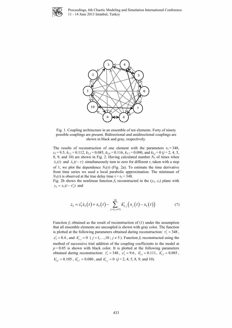
Proceedings, 6th Chaotic Modeling and Simulation International Conference
11 - 14 June 2013 Istanbul, Turkey
Fig. 1. Coupling architecture in an ensemble of ten elements. Forty of ninety possible couplings are present. Bidirectional and unidirectional couplings are
shown in black and gray, respectively. The results of reconstruction of one element with the parameters τ5 = 348, ε5 = 9.5, k5,1 = 0.112, k5,3 = 0.085, k5,6 = 0.116, k5,7 = 0.090, and k5,j = 0 (j = 2, 4, 5, 8, 9, and 10) are shown in Fig. 2. Having calculated number N5 of times when
5 ( )x t and 5 (x t )τ− simultaneously turn to zero for different τ, taken with a step of 1, we plot the dependence N5(τ) (Fig. 2a). To estimate the time derivative from time series we used a local parabolic approximation. The minimum of N5(τ) is observed at the true delay time τ = τ5 = 348. Fig. 2b shows the nonlinear function f5 reconstructed in the (y5, z5) plane with
5 5 5(y x t )τ ′= − and
( ) ( ) ( ) ( )(10
5 5 5 5 5 51( 5)
, j jj j
z ε x t x t k x t x t= ≠
′ ′= + − −∑ ) (7)
Function f5 obtained as the result of reconstruction of (1) under the assumption that all ensemble elements are uncoupled is shown with gray color. The function is plotted at the following parameters obtained during reconstruction: 5 348τ ′ = ,
5 8.4ε ′ = , and ( ;5, 0jk ′ = 1, ,10j = … 5j ≠ ). Function f5 reconstructed using the method of successive trial addition of the coupling coefficients to the model at p = 0.05 is shown with black color. It is plotted at the following parameters obtained during reconstruction: 5 348τ ′ = , 5 9.6ε ′ = , 5,1 0.111k ′ = , 5,k 3 0.085′ = ,
, k , and 5,6 0.105k ′ = 5,7 0.0′ = 80 5, jk 0′ = (j = 2, 4, 5, 8, 9, and 10).
433
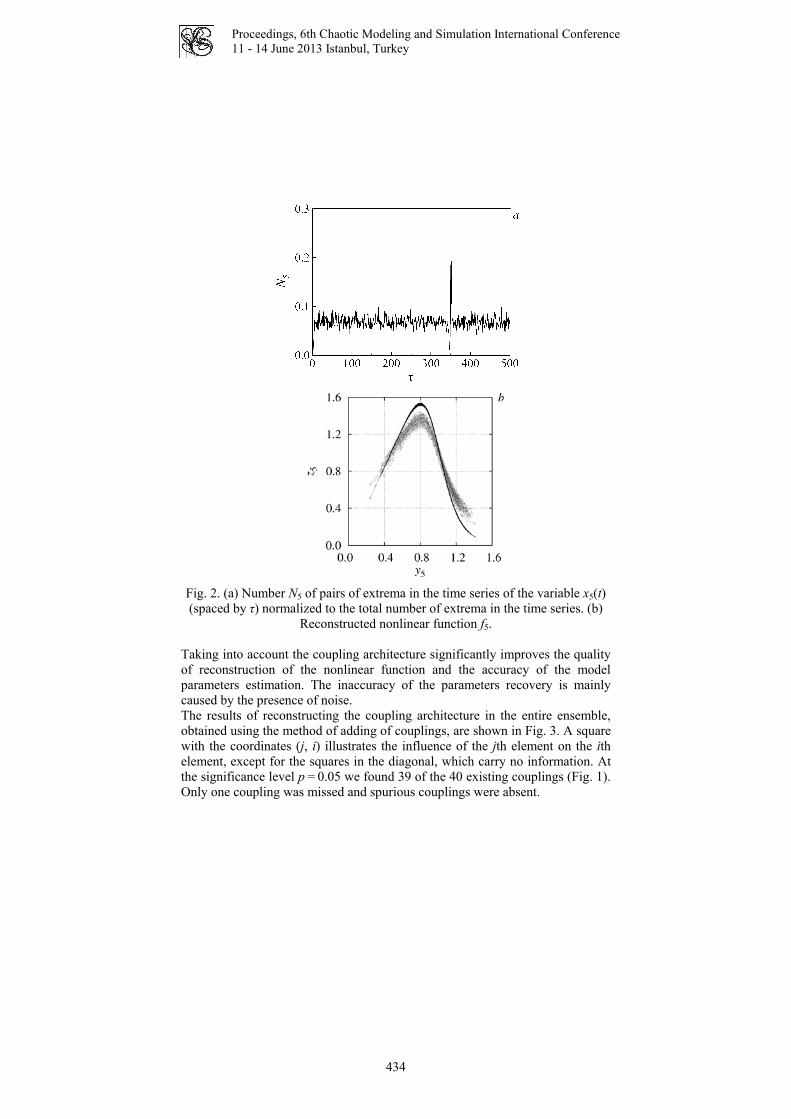
Proceedings, 6th Chaotic Modeling and Simulation International Conference
11 - 14 June 2013 Istanbul, Turkey
Fig. 2. (a) Number N5 of pairs of extrema in the time series of the variable x5(t) (spaced by τ) normalized to the total number of extrema in the time series. (b)
Reconstructed nonlinear function f5. Taking into account the coupling architecture significantly improves the quality of reconstruction of the nonlinear function and the accuracy of the model parameters estimation. The inaccuracy of the parameters recovery is mainly caused by the presence of noise. The results of reconstructing the coupling architecture in the entire ensemble, obtained using the method of adding of couplings, are shown in Fig. 3. A square with the coordinates (j, i) illustrates the influence of the jth element on the ith element, except for the squares in the diagonal, which carry no information. At the significance level p = 0.05 we found 39 of the 40 existing couplings (Fig. 1). Only one coupling was missed and spurious couplings were absent.
434

Proceedings, 6th Chaotic Modeling and Simulation International Conference
11 - 14 June 2013 Istanbul, Turkey
Fig.3. Diagram of the results of recovering the coupling architecture in an ensemble of ten Mackey–Glass systems obtained at the significance level
p = 0.05 using the method of successive trial addition of coupling coefficients to the model. Correctly recovered couplings, correctly found absent couplings, and
missed couplings are shown in black, white, and gray, respectively.
Note that reconstructing the coupling architecture from the same time series using the method of excluding of couplings, we obtained many spurious couplings at the same p. The method of excluding of couplings is more efficient for reconstructing ensembles where the number of existing couplings is many times larger than the number of absent couplings. On the contrary, the method of adding of couplings is most efficient when the number of couplings in an ensemble is small. It works well even in the case of large ensembles (M = 50). The case under consideration, in which the numbers of existing and absent couplings are comparable, is the most complicated for reconstruction. In these situations the method of adding of couplings is more efficient. 3. Conclusions We have proposed the method for the reconstruction of coupling architecture in ensembles of interacting time-delay systems. Besides the coupling values, the method allows one to recover the delay times, parameters of inertia, and nonlinear functions of each element of the ensemble. For the diagnostics of significance of couplings we have used the method of successive trial addition of coupling terms to the model and the method of successive trial exclusion of coupling terms from the model. The method is successfully applied to the reconstruction of the coupling architecture in the ensemble of coupled nonidentical Mackey-Glass systems from chaotic time series of their oscillations.
References 1. A. Pikovsky, M. Rosenblum, and J. Kurths. Synchronization: A Universal Concept in
Nonlinear Sciences, Cambridge: Cambridge University Press, 2001. 2. M. Timme. Revealing network connectivity from response dynamics, Phys. Rev. Lett.,
98: 224101, 2007.
435

Proceedings, 6th Chaotic Modeling and Simulation International Conference
11 - 14 June 2013 Istanbul, Turkey
3. I. T. Tokuda, S. Jain, I. Z. Kiss, and J. L. Hudson. Inferring phase equations from multivariate time series, Phys. Rev. Lett. 99:064101, 2007.
4. D. A. Smirnov and B. P. Bezruchko. Detection of couplings in ensembles of stochastic oscillators, Phys. Rev. E 79: 046204, 2009.
5. M. D. Prokhorov, V. I. Ponomarenko, A. S. Karavaev, and B. P. Bezruchko. Reconstruction of time-delayed feedback systems from time series, Physica D 203:209–223, 2005.
6. V. I. Ponomarenko and M. D. Prokhorov. Estimating characteristics of ensemble of coupled delay-feedback systems from their experimental time series, Tech. Phys. Lett. 36:902–905, 2010.
7. M. Kendall and A. Stuart. The Advanced Theory of Statistics, New York: MacMillan, 1979.
8. N. L. Johnson, S. Kotz, and N. Balakrishnan. Continuous Univariate Distributions, vol. 2, New York: Wiley, 1995.
436

Proceedings, 6th Chaotic Modeling and Simulation International Conference
11 - 14 June 2013 Istanbul, Turkey
Digital Secure Communication Using Chaotic Time-Delay Systems
Mikhail D. Prokhorov, Vladimir I. Ponomarenko, Danil D. Kulminskiy,
Anatoly S. Karavaev
Saratov Branch of the Institute of Radio Engineering and Electronics of Russian Academy of Sciences, Saratov, Russia E-mail: [email protected]
Abstract: We have developed an experimental system for secure communication with nonlinear mixing of information signal and chaotic signal of a time-delay system based on programmable microcontrollers with digital transmission line. The proposed scheme allows one to transmit and receive speech and musical signals in a real time without noticeable distortion. Keywords: Chaotic communication, Time-delay systems, Chaotic synchronization. 1. Introduction The development of communication systems employing the phenomenon of synchronization of chaotic oscillations has attracted a lot of attention [2, 4, 7, 8] due to the broadband power spectrum of chaotic signals, high speed of information transmission, and tolerance to sufficiently high levels of noise. Besides, many chaotic communication schemes are simply realized and demonstrate a rich variety of different oscillating regimes. Different approaches for the transmission of information signals using chaotic dynamics have been proposed. Nonlinear mixing of information signal and chaotic signal is one of the most widespread among them [4]. However, one of the main disadvantages of communication systems with nonlinear mixing is their comparatively low interference immunity [4]. It is explained by the fact that, in order to ensure the security of transmitted data, the level of information signal must be significantly lower than that of the chaotic carrier. Under these conditions, the presence of noise in the communication channel leads to an appreciable distortion of the message signal at the scheme output. We propose a scheme of data transmission with nonlinear mixing, in which the information signal is added to a chaotic signal that is formed as a result of digital calculations on a microcontroller. The receiver, whose parameters are identical with those of the transmitter, receives a digital signal from which the information component is extracted using again digital calculations. Such communication system exploits masking of the information signal by a chaotic signal and possesses sufficiently high stability to noise that is inherent in digital systems of data transmission. In order to increase the level of security of hidden data transmission it has been proposed to employ time-delay systems, demonstrating chaotic dynamics of very high dimension, in private communication [5, 6, 9, 11]. For this reason, we
437

Proceedings, 6th Chaotic Modeling and Simulation International Conference
11 - 14 June 2013 Istanbul, Turkey
have considered in the present paper a communication scheme with nonlinear mixing based on chaotic oscillator with delayed feedback. 2. Communication Scheme A block diagram of the communication system with nonlinear mixing is shown in Figure 1. A transmitter represents a ring system composed of a delay line, a nonlinear element, and a linear low-pass filter. The information signal m(t) is added to the chaotic signal f(x(t–τ)) with the help of a summator and the signal s(t) = f(x(t–τ))+m(t) is transmitted into the communication channel and simultaneously injected into the feedback circuit of the transmitter whose dynamics is described by a first-order delay-differential equation
( )( ) ( ) ( ) ( )x t x t f x t m tε = − + − +τ , (1) where x(t) is the system state at time t, f is a nonlinear function, τ is the delay time, and ε is a parameter that characterizes the inertial properties of the system. With this nonlinear mixing the information signal is directly involved in the formation of a complicated dynamics of the chaotic system.
Fig. 1. Block diagram of the communication system with nonlinear mixing: (I) transmitter, (II) receiver, (DL) delay lines, (ND) nonlinear devices, and
(F) filters. A receiver is composed of the same elements as the transmitter, except for the summator that is replaced by a subtracter breaking the feedback circuit. The receiver equation is
( )( ) ( ) ( ) ( )y t y t f x t m tε = − + − +τ . (2) At the output of the subtracter we have the extracted information signal m’(t) = f(x(t–τ))+m(t)– f(y(t–τ)). If the transmitter and the receiver are
438

Proceedings, 6th Chaotic Modeling and Simulation International Conference
11 - 14 June 2013 Istanbul, Turkey
composed of identical elements, they become completely synchronized after the transient process. The difference between the oscillations of systems (1) and (2), Δ(t) = x(t)–y(t), decreases in time for any ε>0, since ( ) ( )t t εΔ = −Δ . As the result of synchronization we have x(t) = y(t) and, hence, f(x(t–τ)) = f(y(t–τ)) and m’(t) = m(t) . It should be noted, that the quality of the extraction of message m(t) does not depend on its amplitude and frequency characteristics. By this is meant that the considered communication scheme allows one to transmit complicated information signals without distortion. The nonlinear element in our scheme provides a quadratic transformation. In this case the transmitter equation takes the form
( )2( ) ( ) ( ) ( )x t x t x t m tε λ τ= − + − − + , (3) where λ is the parameter of nonlinearity. The transmitter parameters were chosen to obtain a regime of developed chaotic oscillations. We used a programmable microcontroller to implement the transmitter. Since this device has no built-in facilities supporting the floating-point operations, one should use integer calculations in microcontroller in order to increase the speed of response. For this purpose the variables and parameters of Eq. (3) were scaled as follows. For small ε, the allowable limits of variation of the parameter λ for which system (3) has a periodic or chaotic attractor are from 0 to 2. Within this range of λ variation the dynamical variable x(t) can take values from –2 to +2. Let us pass to integer arithmetic and transform Eq. (3) in such a way that the dynamical variable would be placed in a 16-bit memory location, whereby its integer values vary between –215 and 215. It can be done by substituting variables as X(t) = 214x(t) and M(t) = 214m(t). Then, Eq. (3) takes the following form:
2
14 14 14 14
( ) ( ) ( ) ( )2 2 2 2X t X t X t Mε τλ −⎛ ⎞= − + − +⎜ ⎟
⎝ ⎠t . (4)
Multiplying both sides of Eq. (4) by 214 and introducing parameter Λ = 214λ, we obtain the following equation:
2
14
( ( ))( ) ( ) ( )2
X tX t X t M tτε −= − + Λ − + . (5)
This differential equation can be reduced to a difference equation, which is more convenient for program implementation on a microcontroller:
(1 1 (n n n kt t )) nX X F X Mε ε+ −Δ Δ⎛ ⎞= − + +⎜ ⎟
⎝ ⎠, (6)
439

Proceedings, 6th Chaotic Modeling and Simulation International Conference
11 - 14 June 2013 Istanbul, Turkey
where n is the discrete time, Δt is the time step, k is the discrete delay time in units of sampling time Δt, and 2 1( ) 2n k n kF X X− −= Λ − 4 . Figure 2 shows a block diagram of the transmitter based on a programmable microcontroller. At the first step of microcontroller program operation the circular buffer array (containing the values from Xn – k to Xn) is initialized by a certain constant value as the initial condition. Then, the nonlinear function F(Xn – k) is calculated and summed with the information signal Mn. After that, the obtained sum Sn is transmitted into the communication channel that is organized as a serial digital interface. The subsequent value of the discrete dynamic variable Xn + 1 is calculated in accordance with relation (6) and fed into the circular buffer. After k cycles the process of initialization is accomplished and the buffer is filled by actual values.
Fig. 2. Block diagram of the transmitter implemented on a microcontroller: (Σ) summator, a and b are constant multipliers, where a = 1–Δ t/ε and b = Δ t/ε.
The linear transformation of the signal in our scheme was performed using a digital low-pass first-order Butterworth filter. It should be noted that employment of high-order filters with an infinite or finite pulse characteristic usually allows one to increase the security of the communication scheme. The greater the number of coefficients in the equation that describes the filter, the greater the number of previous values of the variable involved in calculations of the next value and, hence, the higher the security level of transmitted data. The nonlinear transformation can also be of various types. For example, one can use a Bernoulli map, a tent map, or other maps with chaotic dynamics. 3. Extracting Information Signal Mixed with Chaotic Signal In our scheme the transmitter was implemented on a programmable microcontroller of the Atmel megaAVR family. As the information signal we choose a musical information signal (a song). Part of the time series of this audio signal is presented in Figure 3(a). The analog information signal m(t) is fed to the input of an analog-to-digital converter (ADC) and the signal Mn from its output is mixed with the chaotic signal of the transmitter. The calculations are performed in terms of integer arithmetic, with the chaotic signal amplitude varying within 16 bits and the information signal within 12 bits.
440

Proceedings, 6th Chaotic Modeling and Simulation International Conference
11 - 14 June 2013 Istanbul, Turkey
Fig. 3. (a) Oscillograms of temporal realizations of musical information signal m(t) at the transmitter input (on top) and the extracted information signal m’(t) at the receiver output (below). (b) Time series of chaotic signal Sn. (c) Power
spectra of signals Mn (1), Sn (2), and Mn’ (3). The spectrum of Mn’ is shown by grey color.
Figure 3(b) shows a part of the time series of a chaotic signal Sn = F(Xn – k)+Mn generated by the oscillator with delayed feedback at λ = 1.9, Δt/ε = 0.5, and k = 100. This signal had a digitization frequency of 20 kHz (Δt = 50 mcs) and was transmitted over a digital communication channel at a rate of 115.2 kbit/s using RS-232 interface. If one passes this signal through a digital-to-analog converter (DAC) and reproduce, he will hear only noise without any signs of speech and music. The receiver was implemented on the same programmable microcontroller as the transmitter. At the subtracter output of the receiver we have the extracted information signal Mn’ = F(Xn – k)+Mn–F(Yn – k) . If the receiver parameters are identical with those of the transmitter and noise is absent, then F(Yn – k) = F(Xn – k) and Mn’ = Mn . Passing the digital signal Mn’ through a DAC we obtain the analog information signal m’(t) at its output. Part of the time series of m’(t) is also displayed in Figure 3(a). As it can be seen from Figure 3(a), the time series of the original and extracted information signals are very similar. Aurally the original musical signal m(t) and the signal m’(t) at the receiver output are indistinguishable.
441

Proceedings, 6th Chaotic Modeling and Simulation International Conference
11 - 14 June 2013 Istanbul, Turkey
Figure 4(c) shows the power spectra of the chaotic signal Sn, musical information signal Mn, and the signal Mn’ extracted in the receiver. The amplitude of the musical information signal comprises about 25% of the amplitude of the chaotic carrier and the presence of audio signal is not noticeable in the power spectrum of the transmitted signal Sn. The power spectra of the signals Mn and Mn’ are very close. Thus, the quality of hidden information extraction at the receiver output is good enough in spite of the presence of noise inherent in a real system. The proposed scheme allows one to transmit and receive speech and musical signals in a real time without noticeable distortion. 4. Extraction of Information Signal at the Mismatch of the Receiver and Transmitter Parameters In the example considered in the previous section the identity of the parameter values in the transmitter and receiver ensures the high quality of hidden message extraction for the authorized listener. The identity of the receiver and transmitter parameters is very important for communication schemes based on synchronization of chaotic systems. With the increase of mismatch of the receiver and transmitter parameters, the quality of chaotic synchronous response of the receiver deteriorates leading to a worse quality of the information signal extraction [4]. Beginning with a certain value of mismatch, the extraction of hidden message becomes impossible. The advantage of the proposed digital communication scheme is the employment of programmable microcontrollers that allows us to achieve the complete identity of the receiver and transmitter parameters, which is practically unattainable in the case of constructing the receiver and transmitter from analog elements. For an eavesdropper the signal transmitted over the communication channel is perceived as noise. To extract a hidden message from the chaotic carrier the unauthorized listener must know the transmitter configuration, i.e. he must know that the transmitter is governed by the model time-delay equation (1) and he must know also the type of nonlinear function f and accurate values of the system parameters. For reconstruction of model equations of time-delay systems and estimation of their parameters from time series a number of methods has been proposed [1, 3, 10, 12]. In the absence of noise these methods allow one to recover the unknown parameters of time-delay systems with a good accuracy. However, in the presence of noise the parameter estimation is less accurate. Moreover, the error of parameter estimation increases with the increase of noise level. The considered communication scheme employs nonlinear mixing of information signal and chaotic signal of a time-delay system. In this case the presence of information signal in the chaotic carrier inevitably decreases the accuracy of estimation of the system parameters just as in the case of noise presence. We have examined how accurately the transmitter parameters must be known for extracting a hidden information signal at the receiver output. Let us choose the same transmitter parameters as in Section 3 and the same musical information signal. The receiver parameters are chosen the same as for
442

Proceedings, 6th Chaotic Modeling and Simulation International Conference
11 - 14 June 2013 Istanbul, Turkey
transmitter except for the discrete delay time k, which is varied in the vicinity of true value of k = 100. Already for a minimal mismatch of k by unity (k = 99 or k = 101) we hear only noise at the receiver output. Thus, the information signal is completely masked in the case of a 1% mismatch of the delay time in the transmitter and receiver. Parts of the time series of the original musical signal m(t) and the signal m’(t) extracted in the receiver at k = 99 are presented in Figure 4. The amplitude of the signal m’(t) is significantly greater than the amplitude of m(t). Besides, the signal m’(t) looks like a chaotic carrier.
Fig. 4. Oscillograms of temporal realizations of the original information signal m(t) (on top) and the information signal m’(t) extracted in the receiver at the
mismatch of parameter k (k = 99) (below). We study also the influence of the parameter e mismatch on the quality of the hidden message extraction. The receiver and transmitter parameters are chosen the same except for the parameter ε, which is varied in the vicinity of true value of ε = 100 mcs. It is found out that the information signal is not heard at the receiver output if a mismatch of ε is greater than 1.5%. In this case the time series and power spectra of m’(t) and m(t) are appreciably different. In the case of 0.1-1% mismatch by ε, the information signal is masked partially. We can distinguish several words and a musical background at the receiver output although the time series and power spectra of m’(t) and m(t) are appreciably different. If a mismatch of ε is 0.05%, the musical signal is extracted in the receiver with a small noise disturbance, which disappears under the further decrease of mismatch. Thus, in order to extract a hidden message an authorized listener has to reconstruct the transmitter parameters with a high accuracy that is a very complicated problem for the proposed scheme. 5. Conclusion We have developed the experimental digital communication system with nonlinear mixing of information signal and chaotic signal of time-delay system in which the transmitter and receiver are implemented on programmable microcontrollers. This system allows one to transmit and receive speech and
443

Proceedings, 6th Chaotic Modeling and Simulation International Conference
11 - 14 June 2013 Istanbul, Turkey
musical signals in a real time without noticeable distortion. The high quality of hidden message extraction is achieved due to the use of digital elements in the scheme, which ensure identity of the parameters and high stability to noise typical for digital communication systems. We have studied a possibility of extraction of hidden information signal in the case of mismatch of the parameters of the receiver and transmitter in the proposed scheme. It is found out that for the hidden message extraction the parameter mismatch must be less than 1% that ensures the privacy of the proposed communication scheme. Acknowledgements This work is supported by the Russian Foundation for Basic Research, Grant No. 13-02-00227 and by the grant of the president of Russian Federation, MK-4435.2012.8. References 1. M. J. Bünner, M. Ciofini, A. Giaquinta, R. Hegger, H. Kantz, R. Meucci and A. Politi.
Reconstruction of systems with delayed feedback: (I) Theory. Eur Phys J D 10:165–176, 2000.
2. K. M. Cuomo and A. V. Oppenheim. Circuit implementation of synchronized chaos with applications to communications. Phys Rev Lett 71:65–68, 1993.
3. C. Dai, W. Chen, L. Li, Y. Zhu and Y. Yang. Seeker optimization algorithm for parameter estimation of time-delay chaotic systems. Phys Rev E 83:036203, 2011.
4. A. S. Dmitriev and A.I. Panas. Dynamical Chaos: New Information Carriers for Communication Systems. Fizmatlit, Moscow, 2002.
5. W.-H. Kye. Information transfer via implicit encoding with delay time modulation in a time-delay system. Phys Lett A 376:2663–2667, 2012.
6. R. M. Nguimdo, P. Colet, L. Larger and L. Pesquera. Digital key for chaos communication performing time delay concealment. Phys Rev Lett 107:034103, 2011.
7. U. Parlitz, L. O. Chua, L. Kocarev, K. S. Halle and A. Shang. Transmission of digital signals by chaotic synchronization. Int J of Bifurcation and Chaos 2:973–977, 1992.
8. L. M. Pecora, T. L. Carroll, G. A. Johnson, D. J. Mar and J. F. Heagy. Fundamentals of synchronization in chaotic systems, concepts, and applications. Chaos 7:520–543, 1997.
9. V. I. Ponomarenko and M. D. Prokhorov. Extracting information masked by the chaotic signal of a time-delay system. Phys Rev E 66:026215, 2002.
10. M. D. Prokhorov, V. I. Ponomarenko, A. S. Karavaev and B. P. Bezruchko. Reconstruction of time-delayed feedback systems from time series. Physica D 203:209–223, 2005.
11. K. Pyragas. Transmission of signals via synchronization of chaotic time-delay systems. Int J of Bifurcation and Chaos 8:1839–1842, 1998.
12. L. Zunino, M. C. Soriano, I. Fischer, O. A. Rosso and C. R. Mirasso. Permutation-information-theory approach to unveil delay dynamics from time-series analysis. Phys Rev E 82:046212, 2010.
444

Proceedings, 6th Chaotic Modeling and Simulation International Conference
11 - 14 June 2013 Istanbul, Turkey
Acceleration Data Extraction Associating to
the Peak-Valley Segmentation Approach
Using the Morlet Wavelet Transform
S. Abdullaha1
, T. E. Putraa2
, D. Schrammb3
, M. Z. Nuawia4
aDepartment of Mechanical and Materials Engineering,
Universiti Kebangsaan Malaysia
43600 UKM Bangi Selangor, Malaysia bDepartmental Chair of Mechatronics,Universität Duisburg-Essen
47057 Duisburg, Germany
E-mail: [email protected],
Abstract: This paper presents a peak-valley segmentation procedure for the wavelet-
based extraction of acceleration data. A 60-second acceleration signal was measured on a
McPherson frontal coil spring of a 2000 cc Proton sedan car, and the data was used for
the simulation. The Morlet wavelet-based analysis was used to extract higher amplitude
segments in order to produce a shortened signal that has an equivalent behaviour. Using
this process, it has been found that the Morlet wavelet was able to summarise the original
data up to 49.45% with less than 10% difference with respect to statistical parameters.
This clearly indicates that the Morlet wavelet can be successfully applied to compress the
original signal without changing the main history as well. Finally, it has been proven that
the Morlet wavelet successfully identified the higher amplitudes in the acceleration data.
Keywords: Acceleration data, Peak-valley extraction, Morlet wavelet, Modified data.
1. Introduction Control and stability of a car entirely depend on the contact between the road
surface and the tires [1]. The dynamic interaction between vehicle and road
surface causes problems with respect to the vehicle structure and the ride
quality. Collision between uneven road surfaces and tires gives a certain amount
of vibration which contributes to mechanical failure of car components due to
fatigue as the car structure was subjected to cyclic loading. This vibration also
interfaces the function of the car suspension system and gives a great impact on
the performance of the car [2-5].
According to Jinhee [6], car suspension systems experience vibration when is
subjected to variable driving conditions leading to strain at this component. If
this condition continues it will increase the probability of fatigue failure for the
car suspension system. The problems arising have been solved by simulating the
dynamic behaviour of a structural component on which the dynamic forces are
acting. Measured road surface profiles are generally considered as external
disturbances acting through the automotive suspension system onto the vehicle
body. Road surface profiles are usually used to describe the bumpiness of the
road. Because of weakness of measuring equipment used, there is noise in the
445

Proceedings, 6th Chaotic Modeling and Simulation International Conference
11 - 14 June 2013 Istanbul, Turkey
road surface profile data. Thus, the accuracy and reliability of the road surface
profile is reduced. If the signal trends are not extracted from the input signal
used, it will directly affect the test results, leading to inappropriate judgments
and conclusions. Therefore, it is an important task that the signal trend is
extracted and separated from the noise during road surface data processing [7].
Based on this background, methods for the signal trend extraction of road
surface profile are introduced. At present, the popular methods for the signal
trend extraction are: least-squares fitting, low-pass filtering, wavelet
decomposition, empirical mode decomposition, etc., as reported in [7]. The
objective of this work is to extract acceleration data in order to remove white
noise in the data. In order to address the objective of the research, acceleration
data is edited to produce shorter data while retaining its original characteristics.
Therefore, a data editing technique is necessary for producing new modified
signals as required. Continuous wavelet transform (CWT) has been applied to
the digital signal processing algorithm. An algorithm for signal trend extraction
of road surface profile has been developed by adopting a fatigue feature
algorithm developed by Putra et al [8]. It is hypothesized that the pattern of an
acceleration data is similar to the pattern of a fatigue signal.
2. Literature Overview 2.1. Global signal statistics
Statistical parameters are used for random signal classification and pattern
monitoring. Common statistical parameters that are directly related to the
observation of the data behaviour are the mean value, standard deviation (SD),
the root-mean square (r.m.s.), skewness, kurtosis and the crest factor (CF). From
these parameters, the r.m.s. and kurtosis give significant effects to evaluate the
randomness of the data [9]. The r.m.s. calculates the energy distribution,
wherein higher r.m.s. indicates a higher energy content, which in turn indicates
higher fatigue damage in the signal. On the other hand, kurtosis represents the
continuity of peaks in a time series loading. The peaks also reveal higher fatigue
damage, suggesting that a higher kurtosis indicates higher fatigue damage.
The r.m.s. is the second statistical moment used for determining the total energy
contained in a signal. The r.m.s. of signals with zero mean value is equal to the
SD. The r.m.s. of discrete data can be calculated as follows:
21
1
21...
= ∑=
n
j
jxn
smr
In addition, kurtosis is the fourth statistical moment that is very sensitive to
spikes and it represents the continuation of peaks in a time series loading. The
kurtosis value of a Gaussian normal distribution is close to 3.0. Higher kurtosis
shows that the value is higher compared to the appropriate value in the Gaussian
normal distribution, indicating that only a small proportion of data is closer to
the mean value [10]. The kurtosis for a set of discrete data is formulated as:
446

Proceedings, 6th Chaotic Modeling and Simulation International Conference
11 - 14 June 2013 Istanbul, Turkey
( )∑=
−=n
j
j xxSDn
K1
4
4)(
1
2.2. Continuous Morlet Wavelet Transform
The continuous wavelet transform (CWT) is conducted on each reasonable
scale, producing a lot of data and is used to determine the value of a continuous
decomposition to reconstruct the signal accurately [11]. The Morlet wavelet is
one of the mother wavelets that are involved in the CWT, and it can be
described by the following equation:
( ) ( ) ( )πttt cos 2exp 22βψ −=
By dilation with a (scale factor) and translation with b (position), a son wavelet
can be acquired [12]:
( ) ( ) ( )
−
−−−=
a
btπ
a
bttba cos exp
2
22
,
βψ
Wavelet decomposition calculates the resemblance index, also called the
coefficient, between the signal being analyzed and the wavelet. Generally, the
wavelet coefficient is expressed with the following integral [11]:
( ) ( )( )∫+∞
∞−= dtttfC baba ,, ψ
The Morlet wavelet coefficient indicates the distribution of the internal energy
of the signal in the time-frequency domain [13]. The signal internal energy e can
be expressed as:
( ) ( )2
,, baba Ce =
2.3. Peak-valley segmentation-based signal extraction
Fatigue damage is very sensitive to peak and valley in a time series loading.
Thus, in the extraction, time series data needs to be converted in the form of
peak-valley. For the development of the extraction algorithm, the input required
was the distribution of the magnitude in the time domain obtained by the time-
frequency method. The distribution was decomposed into the time domain
spectrum by taking the magnitude cumulative value for an interval of time.
A gate value was used for the extraction of the damage feature. The gate value
was the energy spectrum variable that maintains the minimum magnitude level.
Segments with magnitudes exceeding the minimum magnitude value were
maintained, whereas the segments with magnitudes less than the minimum
447

Proceedings, 6th Chaotic Modeling and Simulation International Conference
11 - 14 June 2013 Istanbul, Turkey
magnitude value were removed from the signal. The concept refers to the
concept of the cut-off level used in the extraction in the time domain [14].
To obtain the optimum of the gate value, the maintained segments then were
merged with each other to form a shorter modified signal, compared to the
original signal. In the case of global signal statistical parameters, a difference of
10% is used considering that at least 10% of the original signal contains a lower
amplitude cycle leading to the minimum structural damage to obtain a final
signal corresponding to the original signal [15].
3. Methodology Acceleration data measured at a McPherson frontal coil spring of a 2.000 cc
Proton Wira sedan car was used for the current study. At the same time, strain
data on the component was measured as well. The behaviour of both the
acceleration and strain data was to be observed. According to Gillespie [16], the
coil spring of a car at the similar brand of this research was made from
SAE5160 alloy steel. Its properties are tabulated in Table 1 [17].
Table 1. The mechanical properties of the SAE5160 alloy steel.
Properties Values
Modulus of elasticity, E (GPa) 207
Density, ρ (kg/m3) 7.85
Poisson’s ratio, ρ 0.27
An accelerometer was placed at the location of the coil spring showing the
highest stress concentration which was obtained through finite element analysis.
The car was driven on a highway road surface at a velocity of 70 km/h. The
original signal produced by the accelerator was a variable amplitude load
sampled at 500 Hz and recorded using a data acquisition setup, as shown in
Figure 1.
Fig. 1. The data acquisition setup: (a) accelerometer, (b) PXI system.
4. Results and Discussion 4.1. Acceleration data
The collected data contained many small amplitudes and higher frequency
patterns in the signal background. The data is a time domain signal measured at
the coil spring sampled at 500 Hz for 30,000 data points. Therefore the total
(b) (a)
448
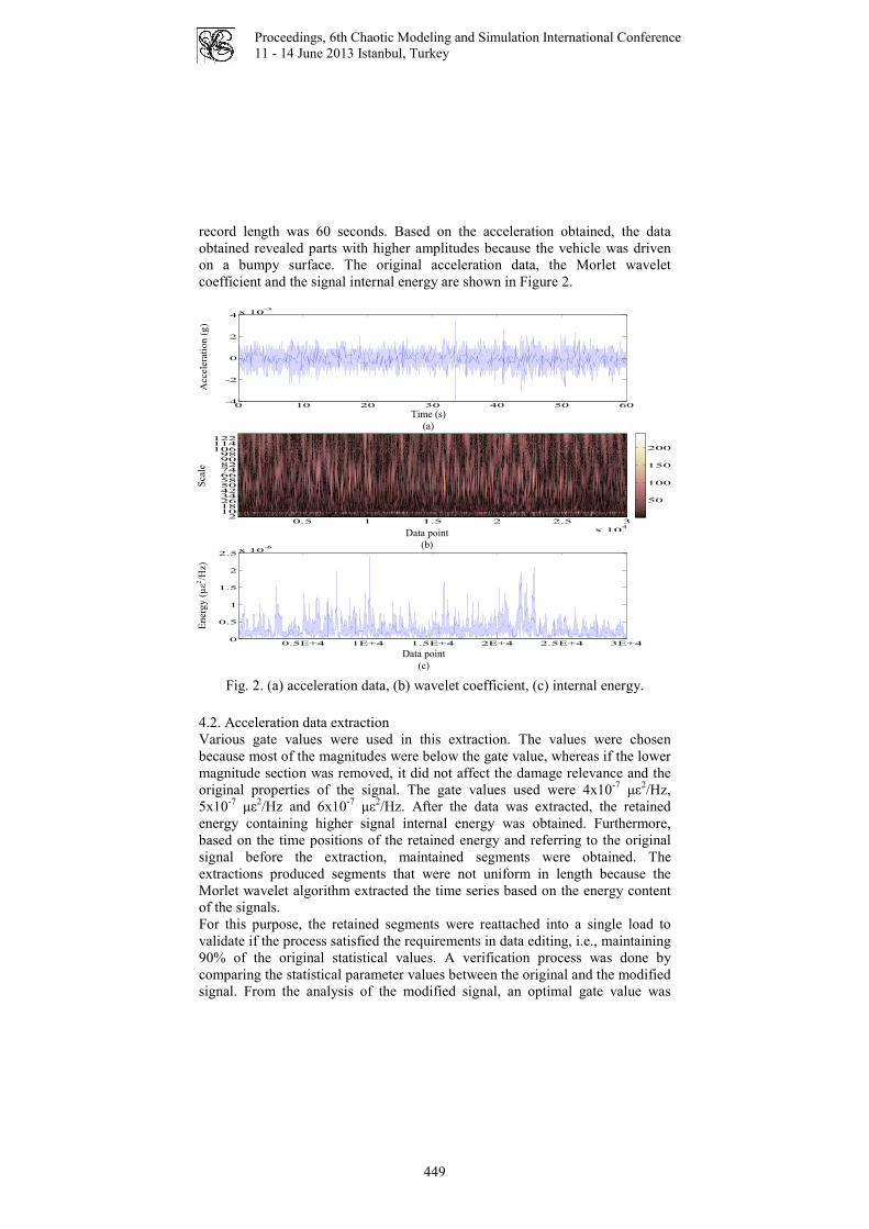
Proceedings, 6th Chaotic Modeling and Simulation International Conference
11 - 14 June 2013 Istanbul, Turkey
record length was 60 seconds. Based on the acceleration obtained, the data
obtained revealed parts with higher amplitudes because the vehicle was driven
on a bumpy surface. The original acceleration data, the Morlet wavelet
coefficient and the signal internal energy are shown in Figure 2.
Fig. 2. (a) acceleration data, (b) wavelet coefficient, (c) internal energy.
4.2. Acceleration data extraction
Various gate values were used in this extraction. The values were chosen
because most of the magnitudes were below the gate value, whereas if the lower
magnitude section was removed, it did not affect the damage relevance and the
original properties of the signal. The gate values used were 4x10⁻⁷
µε2/Hz,
5x10⁻⁷
µε2/Hz and 6x10
-7 µε
2/Hz. After the data was extracted, the retained
energy containing higher signal internal energy was obtained. Furthermore,
based on the time positions of the retained energy and referring to the original
signal before the extraction, maintained segments were obtained. The
extractions produced segments that were not uniform in length because the
Morlet wavelet algorithm extracted the time series based on the energy content
of the signals.
For this purpose, the retained segments were reattached into a single load to
validate if the process satisfied the requirements in data editing, i.e., maintaining
90% of the original statistical values. A verification process was done by
comparing the statistical parameter values between the original and the modified
signal. From the analysis of the modified signal, an optimal gate value was
Acc
eler
atio
n (
g)
Time (s)
(a)
0 10 20 30 40 50 60-4
-2
0
2
4x 10
-3
Sca
le
Data point
(b)
(b)
0.5 1 1.5 2 2.5 3
x 104
2 10 18 26 34 42 50 58 66 74 82 90 98106114122
50
100
150
200
En
erg
y (
µε2
/Hz)
Data point
(c)
0.5E+4 1E+4 1.5E+4 2E+4 2.5E+4 3E+40
0.5
1
1.5
2
2.5x 10
-6
449
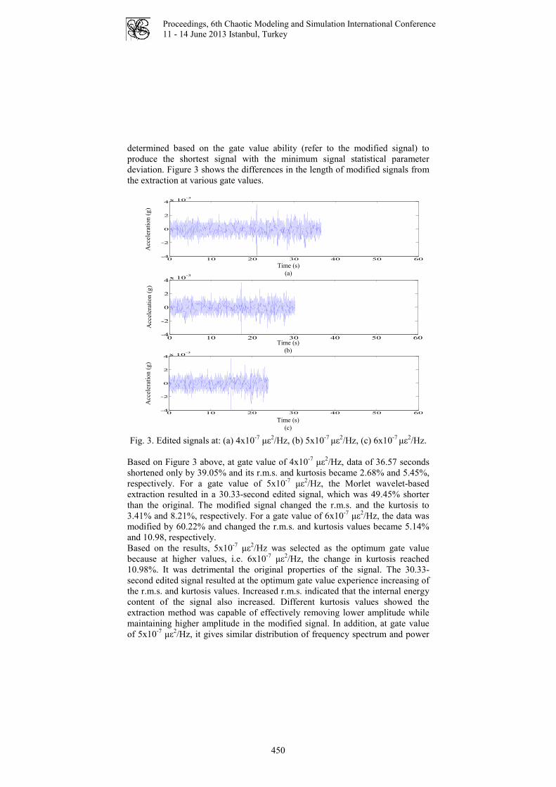
Proceedings, 6th Chaotic Modeling and Simulation International Conference
11 - 14 June 2013 Istanbul, Turkey
determined based on the gate value ability (refer to the modified signal) to
produce the shortest signal with the minimum signal statistical parameter
deviation. Figure 3 shows the differences in the length of modified signals from
the extraction at various gate values.
Fig. 3. Edited signals at: (a) 4x10⁻⁷
µε2/Hz, (b) 5x10
-7 µε
2/Hz, (c) 6x10
-7 µε
2/Hz.
Based on Figure 3 above, at gate value of 4x10⁻⁷
µε2/Hz, data of 36.57 seconds
shortened only by 39.05% and its r.m.s. and kurtosis became 2.68% and 5.45%,
respectively. For a gate value of 5x10⁻⁷
µε2/Hz, the Morlet wavelet-based
extraction resulted in a 30.33-second edited signal, which was 49.45% shorter
than the original. The modified signal changed the r.m.s. and the kurtosis to
3.41% and 8.21%, respectively. For a gate value of 6x10⁻⁷
µε2/Hz, the data was
modified by 60.22% and changed the r.m.s. and kurtosis values became 5.14%
and 10.98, respectively.
Based on the results, 5x10⁻⁷
µε2/Hz was selected as the optimum gate value
because at higher values, i.e. 6x10⁻⁷
µε2/Hz, the change in kurtosis reached
10.98%. It was detrimental the original properties of the signal. The 30.33-
second edited signal resulted at the optimum gate value experience increasing of
the r.m.s. and kurtosis values. Increased r.m.s. indicated that the internal energy
content of the signal also increased. Different kurtosis values showed the
extraction method was capable of effectively removing lower amplitude while
maintaining higher amplitude in the modified signal. In addition, at gate value
of 5x10⁻⁷
µε2/Hz, it gives similar distribution of frequency spectrum and power
Acc
eler
atio
n (
g)
Time (s)
(a)
0 10 20 30 40 50 60-4
-2
0
2
4x 10
-3
Acc
eler
atio
n (
g)
Time (s)
(b)
0 10 20 30 40 50 60-4
-2
0
2
4x 10
-3
Acc
eler
atio
n (
g)
Time (s)
(c)
0 10 20 30 40 50 60-4
-2
0
2
4x 10
-3
450

Proceedings, 6th Chaotic Modeling and Simulation International Conference
11 - 14 June 2013 Istanbul, Turkey
spectral density, as shown in Figure 4. It shows the noise in the road surface
profile had been removed. The data were successfully edited based on the
relationship between the higher amplitude and the Morlet wavelet coefficients
of the time-frequency domain obtained. This Morlet wavelet algorithm removed
segments with magnitudes less than the gate value based on their positions on
the time axis.
Fig. 4. Original and edited signals: (a) length, (b) frequency spectrum,
(c) power spectral density.
5. Conclusion In this study, an experiment was conducted to collect data for the purpose of
obtaining acceleration data to simulate the extraction algorithm. The
acceleration data causes vibration that will increase the probability to the fatigue
failure at car components. The extraction process yielded data on the damaging
segments by identifying and extracting segments based on the coefficient
distribution of the Morlet wavelet transform. The damaging segments were
combined to form shorter signals while maintaining original behaviours.
Overall, the Morlet wavelet algorithm was able to shorten the signal up to
49.45% but maintained more than 90% of the statistical parameters and gave
similar distribution of power spectral density as original data. The extraction
method was able to identify the structural damage values of each segment.
Finally, this study proved that the Morlet wavelet is an appropriate technique to
extract acceleration data, especially for the automotive applications.
Acc
eler
atio
n (
g)
Time (s)
(a)
10 20 30 40 50 60
-3
-2
-1
0
1
2
3
x 10-3
Original
Extracted
Am
pli
tud
e (g
2/H
z)
Frequency (Hz)
(b)
0 50 100 150 200 250
0.2
0.4
0.6
0.8
1
1.2
Original
Extracted
Am
pli
tud
e (g
2/H
z)
Frequency (Hz)
(c)
0 50 100 150 200 250
1
2
3
4
5
6x 10
-8
Original
Extracted
451

Proceedings, 6th Chaotic Modeling and Simulation International Conference
11 - 14 June 2013 Istanbul, Turkey
References
1. C. Ferreira, P. Ventura, R. Morais, A. L. G. Valente, C. Neves and M. C. Reis,
Sensing methodologies to determine automotive damper condition under vehicle
normal operation, Sensors and Actuators A: Physical 156:237-244, 2009.
2. V. Yildirim, Free vibration characteristics of composite barrel and hyperboloidal coil
springs, Mechanics Composite Materials and Structures 8:205-217, 2001.
3. V. Yildirim, A parametric study on the natural frequencies of unidirectional
composite conical springs, Communications in Numerical Methods in Engineering
20:207-227, 2004.
4. S. Narayanan and S. Senthil, Stochastic optimal active control of a 2-dof quarter car
model with non-linear passive suspension elements, Journal of Sound and
Vibration 211:495-506, 1998.
5. L. Sun, Optimum design of ‘‘road-friendly’’ vehicle suspension systems subjected to
rough pavement surfaces, Applied Mathematical Modelling 26:635-652, 2002.
6. L. Jinhee, Free vibration analysis of cylindrical helical springs by the pseudospectral
method, Journal of Sound and Vibration 302:185-196, 2007.
7. D. Hu-ming, X. Fei, Z. Kaibin, M. Ying and S. Feng. Signal trend extraction of road
surface profile measurement, 2nd International Conference on Signal Processing
Systems (ICSPS) 694-698, 2010.
8. T. E. Putra, S. Abdullah, M. Z. Nuawi and Z. M. Nopiah. Wavelet coefficient
extraction algorithm for extracting fatigue features in variable amplitude loading,
Journal of Applied Sciences 10:277-283, 2010.
9. V. Pakrashi, B. Basu, A. O’ Connor, Structural damage detection and calibration
using a wavelet-kurtosis technique, Engineering Structures 29:2097-2108, 2007.
10. C. Braccesi, F. Cianetti, G. Lori and D. Pioli. The frequency domain approach in
virtual fatigue estimation of non-linear systems: the problem of non-Gaussian
states of stress, International Journal of Fatigue 31:766-775, 2009.
11. M. Misiti, Y. Misiti, G. Oppenheim and J. M. Poggi. Matlab User’s Guide: Wavelet
ToolboxTM 4, The Math Works Inc., MA, 2008.
12. J. Lin and L. Qu. Feature extraction based on morlet wavelet and its application for
mechanical fault diagnosis Journal of Sound and Vibration, 234:135-148, 2000.
13. A. K. Darpe. A novel way to detect transverse surface crack in a rotating shaft,
Journal of Sound and Vibration 305:151-171, 2007.
14. R. I. Stephens, P. M. Dindinger and J. E. Gunger. Fatigue damage editing for
accelerated durability testing using strain range and SWT parameter criteria,
International Journal of Fatigue 19:599-606 1997.
15. J. Giacomin, A. Steinwolf and W. J. Staszewski. Application of Mildly
Nonstationary Mission Synthesis (MNMS) to automotive road data, ATA 7th Int.
Conf. on the New Role of Experimentation in the Modern Automotive Product
Development Process 2001.
16. T. D. Gillespie. Fundamental of Vehicle Dynamics. SAE International, United
Kingdom, 1992.
17. nCode. Ice-Flow: Glyphworks 4.0 Tutorials, nCode International Ltd., Sheffield,
2005.
452
Proceedings, 6th Chaotic Modeling and Simulation International Conference
11 - 14 June 2013 Istanbul, Turkey
Chaotic Pattern Recognition Using the Adachi
Neural Network Modified in a Random Manner
Ke Qin1 and B. J. Oommen2,3
1 University of Electronic Science & Technology of China, Chengdu, China. 611731(E-mail: [email protected])
2 Carleton University, Ottawa, ON, Canada. K1S 5B63 University of Agder, Postboks 509, 4898 Grimstad, Norway.(E-mail: [email protected])
Abstract. This paper deals with achieving chaotic Pattern Recognition (PR) usingthe Adachi Neural Network (AdNN), where the Neural Network (NN) has been mod-ified in a random manner. The Adachi Neural Network is a fascinating NN whichhas been shown to possess chaotic properties, and to also demonstrate AssociativeMemory (AM) and Pattern Recognition (PR) characteristics. Variants of the AdNNhave also been used to obtain other PR phenomena, and even blurring. An unsur-mountable problem associated with the AdNN and the variants referred to above, isthat all of them require a quadratic number of computations. Earlier, in [1], we man-aged to reduce the computational cost significantly by merely using a linear numberof computations by enforcing a Maximum Spanning Tree topology, and a gradientsearch method. However, in the sense of a NNs structure, very few networks possessa linearly connected topology. Instead, most of the “physical” networks includingbiological NNs and Internet networks have the properties of a complex network suchas a random network, small-world network or a scale-free network. In this paper, wemainly consider the issue of how the network topology can be modified by involvingrandomized connections so as to render the new network much closer to “real” NNs.On the other hand, the newly obtained network still possesses strong PR character-istics. To achieves this, we first construct a random network by means of the E-Rmodel and then address the problem of computing the weights for the new network.This is done in such a manner that the modified random connection-based NN hasapproximately the same input-output characteristics, and thus the new weights arethemselves calculated using a gradient-based algorithm. Through a detailed exper-imental analysis, we show that the new random AdNN-like network possesses PRproperties for appropriate settings. As far as we know, such a random AdNN has notbeen reported, and our present results are novel.Keywords: Chaotic Neural Networks, Chaotic Pattern Recognition, Adachi-likeNeural Networks, Random Networks.
1 Introduction
The use of Artificial Neural Networks (ANNs) is one of the four best approachesfor Pattern Recognition (PR). ANNs attempt to use some organizational prin-ciples such as learning, generalization, adaptivity, fault tolerance, distributedrepresentation, and computation in order to achieve the recognition. One of thelimitations of most ANN models is the dependency on an external stimulation.Once an output pattern has been identified, the ANN remains in that state
453

Proceedings, 6th Chaotic Modeling and Simulation International Conference
11 - 14 June 2013 Istanbul, Turkey
until the arrival of a new external input. This is in contrast to real biologicalNNs which exhibit sequential memory characteristics. To be more specific, oncea pattern is recalled from a memory location, the brain is not “stuck” in it;it is also capable of recalling other associated memory patterns without beingprompted by any additional external inputs. This ability to “jump” from onememory state to another in the absence of a stimulus is one of the hallmarks ofthe brain, which is one phenomenon that a chaotic PR system has to emulate.
The goal of the field of Chaotic PR systems can be summarized as follows:We do not intend a chaotic PR system to report the identity of a testing patternwith a “class proclamation”. Rather, what we want to achieve is to have thechaotic PR system give a strong periodic ormore frequent signal when a patternis recognized. Furthermore, between two consecutively recognized patterns,none of the trained patterns must be recalled. Finally, and most importantly,if an untrained pattern is presented, the system must give a chaotic signal.
This paper deals with the Adachi Neural Network AdNN [2], which pos-sesses a spectrum of very interesting chaotic, AM and PR properties, as de-scribed in [1,3–11]. The fundamental problem associated with the AdNN andits variants are their quadratic computational requirements. We shall showthat by using the E-R model and an effective gradient search strategy, thisburden can be significantly reduced, and yet be almost as effective with regardto the chaotic and PR characteristics.
We are currently working on reducing the complexity of the AdNN and theassociated computations by invoking the so-called “small-world” model.
2 Limitations of the Current Schemes
Although the works of Adachi et al and Calitoiu et al were ground-breaking,it turns out that, as stated in [3–5], the results claimed in the prior workswere not as precise as stated. Apart from this limitation, the computationalburden is excessive, rendering it impractical. Besides this, most of currentNNs have a regular topology, e.g., a completely connected graph or a neighbor-coupled graph. This is in contrast with “real” NNs which usually have irregulartopologies, e.g., a random graph, a small-world graph or even a scale-free graph.The contribution of this paper is to present a novel CNN which is connectedin a randomized AdNN way. For brevity, we refer to the modified AdNN withrandom connections as the “Random-AdNN”.
3 Designing the Random-AdNN
3.1 The Topology of the Random-AdNN
To present the new characteristics of the Random-AdNN, we shall first arriveat a topology with randomly-chosen edges. Such a modified random AdNN isobtained in two steps. Firstly, we connect the neurons by using the E-R model.The second step involves the computation of the weights associated with thisnew structure, which we will address subsequently.
454

Proceedings, 6th Chaotic Modeling and Simulation International Conference
11 - 14 June 2013 Istanbul, Turkey
Algorithm 1 Topology Random-AdNN
Input: N , the number of neurons in the network, and a set of P patterns which thenetwork has to “memorize”.Output: The topology and initial weights of the Random-AdNN.Method:
1: Create a fully-connected graph G with N vertexes which represents the AdNN.2: For each edge, we delete it with a fixed probability, pd.3: Continue this process for all the
(
N
2
)
edges.4: Compute the initial weights of the edges of G, wij as follows:
wij = 1
P
∑P
s=1(2xs
i−1)(2xsj−1), where x
si is the i
th component of the sth pattern.5: If there is no edge between vertex i and j, wij = 0;
End Algorithm Topology Random-AdNN
3.2 The Weights of the Random-AdNN: Gradient Search
Since we have removed most of the “redundant” edges from the completely-connected graph by using the E-R model, it is clear that the NN at hand willnot adequately compare with the original AdNN. Thus, our next task is todetermine a new set of weights so as to force the Random-AdNN to retainsome of its PR properties, namely those corresponding to the trained patterns.We briefly explain below (the details are omitted in the interest of space, andone can refer to [12] for more details) the process for achieving this.
The Random-AdNN is defined by the following equations:
xRi (t+ 1) = f(ηRi (t+ 1) + ξRi (t+ 1)), (1)
ηRi (t+ 1) = kfηRi (t) +
∑
eij∈T
wR∗
ij xRj (t), (2)
ξRi (t+ 1) = krξRi (t)− αxR
i (t) + ai. (3)
where wR∗
ij , xRi , ξRi and ηRi are the weights, outputs, and state variables of
the Random-AdNN respectively, and have similar meanings to wij, xi, ξiand ηi of the AdNN.
In order to find the optimal values of wR∗
ij , we define the square error
between the original output of the AdNN and new output at the nth step as:
Ep =1
2
N∑
i=1
(xA,pi − x
R,pi (n))2, (4)
where xA,pi and x
R,pi imply the outputs of the ith neuron when the pth pattern is
presented to the AdNN network and the Random-AdNN network respectively.The overall global error is defined by E =
∑P
p=1Ep where P is the number of
trained patterns.
In order to adjust wRij to obtain the smallest global error E, we consider the
gradient, ∆wRij , and move wR
ij by an amount which equals ∆wRij in the direction
455
Proceedings, 6th Chaotic Modeling and Simulation International Conference
11 - 14 June 2013 Istanbul, Turkey
where the error is minimized. This can be formalized as follows:
∆wRij = −β
∂E
∂wRij
= −β∂∑P
p=1Ep
∂wRij
= −β
P∑
p=1
∂Ep
∂xR,pi (n)
·∂x
R,pi (n)
∂wRij
= β
P∑
p=1
(xA,pi − x
R,pi (n)) ·
1
ε· xR,p
i (n) · (1− xR,pi (n)) · xR,p
j (n), (5)
where β is the learning rate of the gradient search. The formal algorithm whichachieves the update is given in Algorithm 2.
Algorithm 2 Weights Random-AdNN
Input: The number of neurons, N , a set of P patterns, and the initial weights wRij
of the Random-AdNN. These initial weights are wAij for the edges in the random
graph, and are set to zero otherwise. The parameters and settings which we haveused are the learning rate β = 0.05, ε = 0.015, α = 10, kf = 0.2 and kr = 1.02.Output: The weights wR∗
ij of the Random-AdNN.Method:
1: Compute the outputs of the Random-AdNN corresponding to the P trained in-puts.
2: For all edges of the Random-AdNN, compute ∆wRij as per Equation (5). Other-
wise, set ∆wRij = 0 .
3: wRij ← wR
ij +∆wRij .
4: Go to Step 1 until E is less than a given value or ∆wRij ≈ 0.
End Algorithm Weights Random-AdNN
The results of a typical numerical experiment which proceeds along theabove gradient search are shown in Fig. 1 and 2. In these simulations, wehave chosen the learning rate β to be 0.05. To clarify issues, we catalogueour experiments for three specific cases, namely when the probability pd fordeleting an edge is 0.9, 0.5 and 0.1 respectively.
If pd is 0.9, the total error E and average values of ∆wRij do not converge
to 0, as shown in Fig. 1. However, as pd decreases, e.g., 0.5, then E and ∆wRij
converge to 0, as shown in Fig. 2 (a) and (b). If pd is even less, E and ∆wRij
also converge to 0 but with a faster rate, as shown in Fig. 2 (c) and (d). Thisphenomenon can be easily explained: The larger the value of pd, the smalleris the number of edges and vice versa. Thus, if pd = 0, it means that theRandom-AdNN is exactly the same as the original AdNN. On the other hand,if pd = 1, it means that all the vertexes are isolated and remain as disconnectedunits. Of course, the “fitting” effect that we obtain by the approximate graph,the Random-AdNN, is more precise as the number of edges increases.
The Lyapunov analysis of the Random-AdNN is also available, but omittedhere in the interest of space. It can be found in [12].
456

Proceedings, 6th Chaotic Modeling and Simulation International Conference
11 - 14 June 2013 Istanbul, Turkey
0 10 20 30 40 50−0.35
−0.3
−0.25
−0.2
−0.15
−0.1
−0.05
0
Ave
rage
Val
ue o
f ∆ w
ij
0 10 20 30 40 5030
35
40
45
50
55
60
Tot
al E
rror
E
Time
Fig. 1. The figure on the left shows the variation of the average of ∆wLij (averaged
over all values of i and j) over the first 50 iterations of the gradient search scheme.The average converges to a value arbitrarily close to zero after 12 time steps. Thefigure on the right shows the variation of the global error over the same time frame.Observe that this quantity does not converge to zero.
0 10 20 30 40 50−0.35
−0.3
−0.25
−0.2
−0.15
−0.1
−0.05
0
0.05
Ave
rage
Val
ue o
f ∆ w
ij
0 10 20 30 40 500
1
2
3
4
5
6
7
8
Tot
al E
rror
E
Time
(a) (b)
0 10 20 30 40 50−0.12
−0.1
−0.08
−0.06
−0.04
−0.02
0
0.02
Ave
rage
Val
ue o
f ∆ w
ij
0 10 20 30 40 500
0.1
0.2
0.3
0.4
0.5
0.6
0.7
Tot
al E
rror
E
Time
(c) (d)
Fig. 2. The figures show the variation of the average of ∆wLij and the global error
over the same time frame. The probability of edge deletion is pd = 0.5 (for (a) and(b)) and pd = 0.1 (for (c) and (d)) respectively.
457

Proceedings, 6th Chaotic Modeling and Simulation International Conference
11 - 14 June 2013 Istanbul, Turkey
4 Chaotic and PR Properties of the Random-AdNN
We now briefly report the PR properties of the Random-AdNN. These prop-erties have been discovered as a result of examining the Hamming distancebetween the input pattern and the patterns that appear in the output. Theexperiments were conducted using the Adachi data set described below.
2 4 6 8 10
2
4
6
8
102 4 6 8 10
2
4
6
8
102 4 6 8 10
2
4
6
8
102 4 6 8 10
2
4
6
8
102 4 6 8 10
2
4
6
8
102 4 6 8 10
2
4
6
8
10
Fig. 3. The 10×10 patterns used by Adachi et al . The first four patterns are used totrain the network. The fifth pattern is obtained from the fourth pattern by including15% noise. The sixth pattern is the untrained pattern.
In the ideal setting we would have preferred the Random-AdNN to bechaotic when exposed to untrained patterns, and the output to appear period-ically or more frequently when exposed to trained patterns. Besides yieldingthis phenomenon, the Random-AdNN also goes through a chaotic phase and aPR phase as some of its parameters change.
We summarize the results for the Random-AdNN, obtained by using differ-ent settings of pd. The others parameters are: kf = 0.2, kr = 1.02, α = 10,ε = 0.015, β = 0.05.
From these tables we see clearly that, the Random-AdNN is able to “res-onate” the input patterns with the corresponding output patterns. ConsiderTable 1 (a) as an example. If the input is P1, then the network outputs P1accordingly, and at the same time, no other trained patterns appear in the out-put sequence. Even when a noisy pattern is presented to the system, e.g., P5,which is a noisy pattern of P4 with 15% noise, the network still “resonates” P4instead of P5 in the output sequence. Furthermore, if the input is an untrainedpattern, e.g., P6, then none of the trained patterns will be recalled. Observethat even the input pattern P6, will itself be retrieved only a few times, whichis much less than the other diagonal entries in the table, i.e., when the inputsare P1 – P4. The difference between (a) – (c) is that in Table (c), the network“resonates” the input patterns more frequently than in (a) and (b). This isbecause when pd = 0.1, the Random-AdNN is almost the same as the originalAdNN since the Random-AdNN has most of the edges of the AdNN. However,in this case, the Random-AdNN also needs a quadratic number of computa-tions, which is computationally much more intensive than for the case whenpd = 0.9. In this regard, we comment that pd = 0.9 is good enough for PR,which has only a very small computational burden. By a simple computationwe can see that the expected degree for each vertex of the Random-AdNN isonly N(1 − pd) = 10 for the Adachi data set, which implies that the compu-
458

Proceedings, 6th Chaotic Modeling and Simulation International Conference
11 - 14 June 2013 Istanbul, Turkey
Table 1. The frequency of the Hamming distance between the input and the outputpatterns for the Random-AdNN. The probability pd is 0.9, 0.5, 0.1 for (a), (b), (c)respectively.
Input Patterns
pd = 0.9 P1 P2 P3 P4 P5 P6
P1 151 0 0 0 0 0P2 0 422 0 0 0 0
Retrieved P3 0 0 161 0 0 0Patterns P4 0 0 0 106 177 0
P5 0 0 0 10 2 0P6 0 0 0 0 0 46
Input Patterns
pd = 0.5 P1 P2 P3 P4 P5 P6
P1 202 0 0 0 0 0P2 0 285 0 0 0 0
Retrieved P3 0 0 234 0 0 0Patterns P4 0 0 0 211 206 0
P5 0 0 0 4 3 0P6 0 0 0 0 0 33
(a) (b)
Input Patterns
pd = 0.1 P1 P2 P3 P4 P5 P6
P1 238 0 0 0 0 0P2 0 331 0 0 0 0
Retrieved P3 0 0 258 0 0 0Patterns P4 0 0 0 237 189 0
P5 0 0 0 9 20 0P6 0 0 0 0 0 34
(c)
tational load has been greatly reduced when compared to the original AdNN,which has a vertex degree of 99.
5 Conclusions
In this paper we have concentrated on the field of Chaotic Pattern Recognition(PR), which is a relatively new sub-field of PR. Such systems, which have onlyrecently been investigated, demonstrate chaotic behavior under normal condi-tions, and resonate when it is presented with a pattern that it is trained with.The network that we have investigated is the Adachi Neural Network (AdNN)[2], which has been shown to possess chaotic properties, and to also demon-strate Associative Memory (AM) and Pattern Recognition (PR) characteristics.In this paper we have considered how the topology can be modified so as torender the network much closer to “real” neural networks. To achieve this, wehave changed the network structure to be a random graph, and then computedthe best weights for the new graph by using a gradient-based algorithm. By adetailed experimental suite, we showed that the new Random-AdNN possesseschaotic and PR properties for different settings.
Acknowledgements: The first author would like to thank the Ministry ofScience and Technology of Sichuan Province, China, for its financial support(Grant Nos. 2012HH0003 and 9140A17060411DZ02) for this research.
459

Proceedings, 6th Chaotic Modeling and Simulation International Conference
11 - 14 June 2013 Istanbul, Turkey
References
1.Qin, K., Oommen, B.J.: Adachi-like chaotic neural networks requiring linear-timecomputations by enforcing a tree-shaped topology. IEEE Transactions on NeuralNetworks 20(11) (2009) 1797–1809
2.Adachi, M., Aihara, K.: Associative dynamics in a chaotic neural network. NeuralNetworks 10(1) (1997) 83–98
3.Calitoiu, D., Oommen, B.J., Nussbaum, D.: Desynchronizing a chaotic patternrecognition neural network to model inaccurate perception. Ieee Transactions onSystems Man and Cybernetics Part B-Cybernetics 37(3) (2007) 692–704
4.Calitoiu, D., Oommen, B.J., Nussbaum, D.: Periodicity and stability issues of achaotic pattern recognition neural network. Pattern Analysis and Applications10(3) (2007) 175–188
5.Qin, K., Oommen, B.J.: Chaotic pattern recognition: The spectrum of propertiesof the adachi neural network. In: Lecuture Notes in Computer Science. Volume5342., Florida, USA (2008) 540–550
6.Chen, L., Aihara, K.: Global searching ability of chaotic neural networks. IEEETransactions on Circuits and Systems I: Fundamental Theory and Applications46(8) (1999) 974–993
7.Qin, K., Oommen, B.J.: An enhanced tree-shaped adachi-like chaotic neural net-work requiring linear-time computations. In: The 2nd International Conferenceon Chaotic Modeling, Simulation and Applications, Chania, Greece (2009) 284–293
8.Luo, G.C., Ren, J.S., Qin, K.: Dynamical associative memory: The properties ofthe new weighted chaotic adachi neural network. IEICE TRANSACTIONS onInformation and Systems E95d(8) (2012) 2158–2162
9.Qin, K., Oommen, B.J.: Networking logistic neurons can yield chaotic and patternrecognition properties. In: IEEE International Conference on ComputationalIntelligence for Measure Systems and Applications, Ottawa, Ontario, Canada(2011) 134–139
10.Hiura, E., Tanaka, T.: A chaotic neural network with duffing’s equation. In: Pro-ceedings of International Joint Conference on Neural Networks, Orlando, Florida,USA (2007) 997–1001
11.Qin, K., Oommen, B.J.: The entire range of chaotic pattern recognition propertiespossessed by the adachi neural network. Intelligent Decision Technologies 6(1)(2012) 27–41
12.Qin, K.: Generic Analysis of Chaotic Neural Networks and Their Applicationsin Pattern Recognition and Crypto-systems. PhD thesis. (2010) University ofElectronic Science and Technology of China, Chengdu, China.
460

Proceedings, 6th Chaotic Modeling and Simulation International Conference
11 - 14 June 2013 Istanbul, Turkey
Stochastic Model Reduction for PolynomialChaos Expansion Using Proper Orthogonal
Decomposition
Mehrdad Raisee1, Dinesh Kumar2 and Chris Lacor2?
1 Center of Excellence in Design and Optimization of Energy Systems (CEDOES)School of Mechanical Engineering, College of Engineering, University of Tehran,P.O.Box: 11155-4563, Tehran, IRAN(E-mail: [email protected])
2 Fluid Mechanics and Thermodynamics Research Group, Department ofMechanical Engineering, Vrije Universiteit Brussel, Pleinlaan 2, 1050 Brussels,BELGIUM(E-mail: [email protected], [email protected])
Abstract. In this paper, a non-intrusive stochastic model reduction scheme is de-veloped for polynomial chaos representation using proper orthogonal decomposition.The main idea is to extract the optimal orthogonal basis via inexpensive calculationson a coarse mesh and then use them for the fine discretization analysis. The devel-oped reduced-order model is implemented to the stochastic steady-state heat diffusionequation. The random conductivity field is approximated via the Karhunen-Loeve(KL) expansion. Input random variables are uniformly distributed so that the Gauss-Legendre quadrature scheme is utilized for the numerical integration. The numericalresults showed that the non-intrusive model reduction scheme is able to accuratelyreproduce mean and variance fields. It is found that the computation-time of thereduced-order model is lower than that of the full-order model.Keywords: Uncertainty Quantification, Polynomial Chaos, Reduced-order Model.
1 Introduction
In many engineering applications, uncertainty in physical properties, input dataand model parameters result in uncertainties in the system output. A repre-sentative practical example is design of turbomachineries where uncertaintiesin flow conditions and small variations in structural parameters of compo-nents(e.g. blade profile) can have a significant impact on the performance. Fordesign refinement of such complex mechanical devices, it is necessary to includeall uncertainty information in the output results using uncertainty quantifica-tion (UQ) schemes. However, many complex applications require a fine 3Dcomputational mesh, small time-step and high-dimensional space for stochas-tic analysis. This dramatically increases the computational cost which is notdesirable for design proposes. Thus, it is necessary to employ efficient numericalschemes for stochastic analysis of complex industrial flows. A variety of differ-ent uncertainty quantification methods such as Monte Carlo approach, sensi-tivity method, perturbation method, regression method and polynomial chaos
? Corresponding Author
461

Proceedings, 6th Chaotic Modeling and Simulation International Conference
11 - 14 June 2013 Istanbul, Turkey
have been proposed for uncertainty quantification. All of these techniques havepositive and negative features, and no single technique is optimum for all situ-ations. Following our previous work on UQ (Dinescu et al.[1] and Wang et al.[7]), here we employed Polynomial Chaos (PC) approach to model uncertaintypropagation. Polynomial chaos methods have been successfully applied to solidmechanics problems by several researches (See for example Ghanem and Spanos[3] and Doostan et al. [2]). PC schemes have also been employed for a numberof fluid mechanics problems by a number of researchers such as: Walters andHuyse [6], Mathelin et al. [4] and Dinescu et al. [1]. The polynomial chaos rep-resentation can be used for different Probability Density Functions (PDFs) andcan be implemented through either intrusive or non-intrusive methods. Theintrusive approach requires the modification of the CFD codes and this may bedifficult, expensive, and time consuming for many CFD problems. Moreover,the source codes of most commercial CFD softwares are not accessible and thusit is impossible to implement the intrusive PC approach to such softwares. Forthese reasons, here we focused on non-intrusive PC methodology with uniformPDF for uncertainty quantification. The main shortcoming of all PC methodsis the curse of dimensionality. Developing efficient reduced-order models forshortening the computational cost associated with the stochastic analysis isof great interest for prediction of complex industrial flows with large numberof uncertain parameters. In recent years, several model reduction techniqueshave been proposed for uncertainty quantification. Two informative examplesof such works are: Nouy [5] and Doostan et al. [2]. In Nouy [5] a GeneralizeSpectral Decomposition (GSD) was proposed that gives the reduced basis in-dependent of the stochastic discretization scheme. The GSD implementationto a class of Stochastic Partial Differential Equations (SPDE) leads to drasticcomputational saving though does not circumvent the curse of dimensionality.Doostan et al. [2] proposed an intrusive model reduction technique for chaosrepresentation of a SPDE to tackle the curse of dimensionality. A 2D test casefrom solid mechanics is chosen to illustrate the accuracy and convergence ofthe model.In this work, a non-intrusive reduced-order technique is developed and ap-plied to the 2D steady-state stochastic heat diffusion equation. This paperis organized as follows. In Section 2 we present the details of mathematicalformulation and problem under investigation. In Section 3, the model reduc-tion methodology is described. Finally, in Section 4 the numerical results arepresented and discussed.
2 Mathematical Formulation
To demonstrate the non-intrusive stochastic model reduction algorithm, 2Dsteady-state stochastic heat conduction in a square plate of side 2a is considered(see Figure 1). The 2D heat diffusion with random thermal conductivity isdescribed by the following SPDE:
∂
∂x(k(x, y; ζ)
∂T
∂x) +
∂
∂y(k(x, y; ζ)
∂T
∂y) = 0 (1)
462

Proceedings, 6th Chaotic Modeling and Simulation International Conference
11 - 14 June 2013 Istanbul, Turkey
As shown in Figure (1), the top boundary of the plate is at hot temperature
Fig. 1. Schematic of computational domain.
Th whilst the side and bottom boundaries of the plate are at cold temperatureTc. The thermal conductivity of the plate, k(x, y; ζ), is assumed to be a two-dimensional homogeneous random process with known mean k(x, y) and knowncovariance function:
R(x1, y1;x2, y2) = σk2e−|x1−x2|/bx−|y1−y2|/by (2)
where bx and by are the correlation lengths in x and y directions, respectively,and σk is the standard deviation on the thermal conductivity.A key ingredient here is the representation of stochastic thermal conductivityfield as a Karhunen-Loeve (KL) expansion, a type of Fourier expansion forrandom functions, which amounts to a discretization in the space of randomevents. According to the KL expansion, the eigenvalues and eigenfunctions areobtained by solving the following 2D integral equation:∫
D
R(x1, y1;x2, y2)φn(x2, y2)dx2dy2 = λnφn(x1, y1) (3)
Separation of kernel (2) as R(x1, y1;x2, y2) = σk2e−|x1−x2|/bx .e−|y1−y2|/by and
substitution in (3) leads to two identical 1D integral eigenvalue equations inx and y directions. Solution of the integral equations give eigenvalues (i.e.
λ(x)i and λ
(y)j ) and their corresponding eigenfunctions (i.e. φ
(x)i and φ
(y)j ). As
described in Ghanem and Spanos [3], the complete form of KL expansion forrandom process k(x, y; ζ) is:
k(x, y; ζ) = k(x, y) +
∞∑i=1
∞∑j=1
√λ(x)i λ
(y)j ζi,j
1√2
[φ(x)i (x)φ
(y)j (y) + φ
(x)j (x)φ
(y)i (y)]
(4)
463

Proceedings, 6th Chaotic Modeling and Simulation International Conference
11 - 14 June 2013 Istanbul, Turkey
Having obtained an analytical expression for the thermal conductivity, theSPDE (Equation (1)) is discretized using an explicit central differencing schemein a uniform grid (∆x = ∆y), see Figure 1. Thus, for any set of ζ ≡ ζini=1,first thermal conductivity is calculated in the computational domain using KLexpression (Equation (4)). Then, the new temperature Tn+1 at grid node (i, j)is obtained from old nodal temperature Tn of neighbouring nodes. The solutionis converged when the maximum error between the old and new temperaturevalues is sufficiently small(ε ' 10−9).
3 Model Reduction Methodology
In the classical polynomial chaos expansion, the random temperature fieldT (x, y; ζ) can be decomposed into deterministic and stochastic components.The PC representation of temperature field of order p for n random variableζ ≡ ζini=1 can be written as:
T (x, y; ζ)− < T (x, y) >=
P∑i=1
T i(x, y)ψi(ζ) (5)
where the total number of terms are P + 1 = (p+ n)!/p!n! and the mean valueof T (x, y; ζ) is expressed as:
< T (x, y) >=
∫ω
T (x, y; ζ)f(ζ)dζ (6)
In the above equation, f is Probability Density Function (PDF). Here we as-sumed random variables are uniformly distributed over interval [-1,1] and thusthe PDF is f = 1/2n for n random variables ζini=1. The non-intrusive methoduses spectral projection to find the PC expansion coefficients T i(x, y) in Equa-tion (5). Projecting Equation (5) onto the kth basis and use of orthogonalitygives:
T i(x, y) =1
< ψ2i (ζ) >
∫ω
T (x, y; ζ)ψi(ζ)f(ζ)dζ (7)
The objective of the spectral projection method is to compute the polynomialcoefficients by evaluating numerator in Equation (7) numerically, while thedominator can be computed analytically for multi-variant orthogonal polyno-mials. Here we used the n-dimensional Gauss-Legendre quadrature to computethe projection integrals in Equation (7) as:
T i(x, y) =1
< ψ2i (ζ) >
q∑i1=1
..
q∑in=1
(wi11 ⊗ ..⊗ win
n )T (x, y; ζi11 , .., ζinn )f(ζi11 , .., ζ
inn )
(8)
where (ζk,wk), k = 1, 2, .., q are the one-dimensional (1D) Gauss-Legendreintegration points and weights.
464

Proceedings, 6th Chaotic Modeling and Simulation International Conference
11 - 14 June 2013 Istanbul, Turkey
The above classical expansion dose not represent an optimal PC representationof T (x, y, ζ). To find the optimal PC expansion one can consider the fact thatspatial discretization errors and random discretization errors may be decoupled.Therefore, one can minimize the random discretization errors on the coarse gridand then solve the real physical problem on a fine mesh by using limited numberof optimal random basis zimi=1 (obtained in the coarse grid analysis) where mis the number of dominated eigenvalues. The first step in the model reductionscheme is to find optimal PC basis using POD; a well-known procedure forextracting a basis for a model decomposition from an ensemble of realizations.To this end, suppose in a coarse grid, expression (9) represents an optimal PCexpansion of the stochastic temperature field T (x, y, ζ);
T (x, y; ζ)− < T (x, y) >=
m∑i=1
T i(x, y)zi(ζ) (9)
Now in the coarse grid, the covariance function C(x1, y1;x2, y2) of temperaturefield can be obtained from:
C(x1, y1;x2, y2) =
P∑i=1
T i(x1, y1)T i(x2, y2) < ψ2i > (10)
The corresponding eigenvalues νi and eigenfunctions φi(x, y) are the solutionof the following eigenvalue problem:∫
D
C(x1, y1;x2, y2)φi(x2, y2)dx2dy2 = νiφi(x1, y1) (11)
The upper limit m in the Equation (9) can be found by the size of dominanteigenspace (10) such that
∑mi=1νi/
∑i νi ≥ 0.99.
Having obtained T i(x, y) from classical PC on the coarse grid and eigenfunc-tions φi(x, y) from the solution of eigenvalue problem (11), the set of optimalbasis zimi=1 can be now represented as a linear combination of the set ofclassical polynomial chaos; ψiPi=1 using the following scalar product1:
zi(ζ) = [T (x, y; ζ)− < T (x, y) >,φi(x, y)] =
P∑j=1
αijψj(ζ) (12)
where coefficient αlj are obtained via the scalar product:
αij =
∫R
T j(x, y)φi(x, y)d−→x d−→y (13)
One now dose the classical polynomial chaos on a fine mesh, where zi are usedinstead of ψi. For 1 ≤ i ≤ m, the coefficients in expansion (9) are obtainedfrom:
T i(x, y) =< T (x, y; ζ), zi >
< zi, zi >=
1
νi
P∑j=1
αij < T (x, y; ζ), ψj > (14)
1 The scalar product of functions v and w is defined as: [v, w] =∫xv.wdx.
465

Proceedings, 6th Chaotic Modeling and Simulation International Conference
11 - 14 June 2013 Istanbul, Turkey
4 Results and Discussion
We now examine the performance of the reduced-order model by analyzing the2D steady-state heat conduction equation. It is assumed that the top wall isat Th = 300C and side and bottom walls at Tc = 100C. First, a 2D KLexpansion is performed using the exponential kernel with a standard deviationof σk = 1.0 W/m.K and correlation lengths of bx = by = 10.0 m. The meanthermal conductivity is assumed to be k = 5.0 W/m.K. The first six largestterms in the KL expansions are chosen for further analysis.
Fig. 2. Computed eigenvalues using coarse discretization analysis.
Figures 2 and 3 respectively show the distributions of eigenvalues and | αij |coefficients obtained from the coarse discretization analysis on a 5 × 5 meshwhen a second-order Legendre polynomial (p = 2) is employed. From thesefigures it can be concluded that only two (m = 2) basis functions (i.e. z1 andz2) are adequate for the fine discretization analysis. Thus, fine discretizationanalysis is performed using the new z1 and z2 basis functions on a 40×40 mesh.The computed mean and variance fields using full- and reduced-order modelsare compared in Figure 4. It is visible the fine grid computations via reduced-and full-order models resulted in identical results for the mean temperature.Moreover, full- and reduced-order analysis on the fine mesh produced verysimilar variance fields. The order of maximum difference in variance fields is10−3. The ratio of computation-time for the reduced-order analysis to the timeneeded for the full-order calculation using three fine meshes of 30× 30, 40× 40and 50 × 50 is shown in Figure 5. While reduced-order computations on the30 × 30 results to about 10% saving in the computation-time, more that 50%saving in computation-time is obtained when a finer 50× 50 mesh is employed.
466

Proceedings, 6th Chaotic Modeling and Simulation International Conference
11 - 14 June 2013 Istanbul, Turkey
Fig. 3. Computed | αij | using coarse discretization analysis.
Fig. 4. Comparison of mean and variance fields.
467

Proceedings, 6th Chaotic Modeling and Simulation International Conference
11 - 14 June 2013 Istanbul, Turkey
Fig. 5. Ratio of reduced-order computation-time to the full-order computation-time.
Conclusion
In this paper, a non-intrusive model reduction technique for PC expansion ispresented and discussed. The reduced-order model is applied to the 2D steady-state heat diffusion equation. Distributions of mean and variance obtainedfrom the reduced-order model are compared with those of full-order model.The numerical results show that the developed reduced-order model is able toproduce acceptable results for such statistical quantities. Computation-time ofthe reduced-order model is found to be lower than that of the full-order model.
References
1.C. Dinescu, S. Smirnov, Ch. Hirsch, and C. Lacor. Assessment of intrusive andnon-intrusive non-deterministic CFD methodologies based on polynomial chaosexpansions. Int. J. of Eng. Systems Modeling and Simulation, 2:87-98, 2010.
2.A. Doostan, R. Ghanem, and J. Red-Horse. Stochastic model reduction for chaosrepresentations. Comp. Meth. in Appl. Mech. and Eng., 196:3951-3966, 2007.
3.R. Ghanem, and O. Spanos. Stochastic Finite Elements: A Spectral Approach,1991, Springer Verlag.
4.L. Mathelin, M. Y. Hussaini, and T. A. Zang. Stochastic approaches to uncertaintyquantification in CFD simulations. Numer. Algorithms, 38:209-236, 2007.
5.A. Nouy. A generalized spectral decomposition technique to solve a class of linearstochastic partial differential equations. Comp. Meth. in Appl. Mech. and Eng.,196:4521-4537, 2007.
6.R. W. Walters, and L. Huyse. Uncertainty analysis for fluid mechanics with appli-cations. NASA/CR 2002-211449.
7.X. Wang, Ch. Hirsch, Z. Liu, S. Kang, and C. Lacor. Uncertainty-based robustaerodynamic optimization of rotor blades. Int. J. Numer. Meth. Engng, DOI:10.1002/nme.4438, 2012.
468

Proceedings, 6th Chaotic Modeling and Simulation International Conference
11 - 14 June 2013 Istanbul, Turkey
The profile of temperature in the dissipativeover-dense plasma layer
L. Rajaei1? , S. Miraboutalebi2
1 Physics Department, Qom University, Qom, Iran(E-mail: [email protected])
2 Physics Department, Islamic Azad University, North Tehran Branch, Tehran,1651153311, Iran(E-mail: [email protected])
Abstract. An investigation is undertaken to introduce an effective mechanism ofplasma heating which significantly enhances and facilitates the heating of a denseplasma layer. This mechanism directly related to the phenomena of anomalous trans-parency of a dense plasma layer through the resonant excitation of the coupled surfacewaves. It is shown that the collisional effects reduce the rate of the energy transmis-sion through the plasma layer under resonant conditions. This dissipative effectscause heating of the plasma layer to a considerable amount of temperature. Thetemperature distribution in the plasma layer during the transmission of the electro-magnetic waves is studied.Keywords: Microwave, Dissipation, Incident wave, Over-dense plasma, Surfaceplasma, Transparency.
1 Introduction
The investigations of circumstances and important factors in the plasma heat-ing is the subject of relevance for many fields of plasma physics ranging fromlaboratory experiments to astrophysics [1]. The heat flow and temperaturegradient in plasma are fundamental process that take place during plasma phe-nomenons and are of grate importance effects. These process in some situations,have inevitable destructive effects. One of the challenges of embedding plasmain electric field is the appearance of high temperature electrons which acts likean internal transport barrier. The three well known heating mechanisms ofplasma are ohmic heating, neutral beam injection and high frequency electro-magnetic waves. In the high frequency electromagnetic waves mechanism ofplasma heating, the energy of waves is converted into thermal electron motionthrough electron-ion collisions [2,3]. Also the interaction of the electromagneticwaves with plasma may lead to the resonant excitation of the electrostatic waveswhich subsequently decays generating energetic electrons [4].
In our previous works we studied the total transparency conditions of anoverdense plasma layer due to the resonant excitation of the coupled surfacemodes, [5]-[9]. In the present paper we demonstrate another mechanism ofplasma heating that significantly enhances and facilitates the heating of thedense plasma. We will show that for a collisional plasma under resonant condi-tions, the dissipative effects cause heating of the dense plasma to a considerable
? Corresponding author: Tel +98-25-32854972. E-mail address: [email protected]
469

Proceedings, 6th Chaotic Modeling and Simulation International Conference
11 - 14 June 2013 Istanbul, Turkey
amount of temperature. Hence the process of resonant excitation of the cou-pled plasmons can be considered as an effective mechanism of plasma heating.In fact this process has a dual acting effect, it cause the transparency of theplasma slab and at the same time it gives rise to plasma heating.
This paper is organized as follows: In section two the geometrical construc-tion of the problem and the transmission of the electromagnetic waves throughthe considered structure. In section three the solutions of the heat equationsat steady states condition is given and the temperature is predicted. Finally,section four presents the results.
2 the model
Fig. 1. Schematic diagram showing the spatial distribution of the effective electricpermittivity.
Let us consider a geometrical structure fulfills the conditions under whichthe high transparency of a normally reflected overdense plasma can be observed, [7]. The system is modeled as an overdense plasma layer with length b placedbetween two equal ordinary dielectrics or equivalently cold plasma layer (seeFig. 1). In order to examine the resonant conditions of the excitation of thesurface modes let us consider a p-polarize wave specified by the magnetic fieldcomponent B = (0, 0, Bz) and the electric field in the plane of incidence (x, y),namely E = (Ex, Ey, 0). Considering the geometrical structure of Fig. (1),the spatial part of the electric and the magnetic fields must be proportionalto exp(iky) and the waves amplitudes become functions only of the variable x.In this case the magnetic field and temperature at the steady state, obtain thefollowing forms:
470
Proceedings, 6th Chaotic Modeling and Simulation International Conference
11 - 14 June 2013 Istanbul, Turkey
κ∂2T
∂2x+Q = 0. (1)
ε∂
∂x
1
ε
∂Bz∂x
+ (ε− k2y)Bz = 0 . (2)
where κ refers to the thermal conductivity. Also,
Q =ε02ε′′ωE2
0 |E| , (3)
where ε′′ is the imaginary part of the permittivity. Here ε = (1 − ω2p
ω2s ),
s = (1 + iν/ω), also k0 = ωc and ωp = 4πn0e
2
m . In these equations, all fieldquantities have become dimensionless and redefined as follows:(
r = k0r , t = ωt), E =
E
E0, ν =
ν
ω, T =
T
T0, (4)
where the tilde quantities are dimensionless, but for simplicity, we ignore thetilde sign of our field quantities in equations. Likewise, the temperature shouldsatisfy the surface heat balances. where ky = sinθ. Analytical solutions ofEqs.(2)gives the magnetic field in the both dielectrics and the over dense plasmamediums, and are obtained in the following forms:
Bz = (A1eαx +A2e
−αx), (5)
where α =√k2y − ε. The electromagnetic fields in the vacuum regions, x < −a
and x > b, have the following forms:
Bz = E0eı cos θx +Re−ı cos θx x < −a , (6)
Bz = Treı cos θx x > b , (7)
where E0, R and T respectively assign the field components for the incident,reflected and transmitted waves.
These field solutions should satisfy the conditions of continuity of dBz/dxand Bz, on all the boundaries and as a result, one achieve eight equations forthe unknown coefficients, specifically the coefficient R and Tr are obtained. Forresonant values of the incident angle θ, we should expect anomalous transmis-sion of the electromagnetic waves.
Fig. (2) shows the transmission curve Tr andR as a function of the incidenceangle θ for two different values of the collisional frequencies, namely for ν = 0.1and ν = 0.2. Two important results are obtained from these plots. As the firstresult, there is an acute increase in the transmission properties of the system,when the angle of incidence reaches to one of its resonant values. Accordingto the figure.(2), the maximum of the transmission coefficient T occurs aboutθ = 0.18rad for two different value of collisional frequencies.
As the second result, comparing the two maximums indicates that, with theincrease of the collisional frequency ν, t he maximum rate of the electromagnetic
471

Proceedings, 6th Chaotic Modeling and Simulation International Conference
11 - 14 June 2013 Istanbul, Turkey
Fig. 2. The transmission coefficients vs incident angel for two different value of col-lisional frequency
waves decreases. In order to investigate the effect of this dissipated energy onthe increase of the plasma temperature, the electric field amplitude in the over-dense plasma at the maximum points is needed. To provide this we note thatfor the case ν = 0.1, the deficiency at the maximum point is about 1 − (|R |2 + | Tr |2) = 0.3071, while For the case ν = 0.2 the deficiency is about1− (R2 + T 2
r ) = 0.4373.
3 The heat equation
In order to investigate the temperature variations or the increase of the tem-perature degree of the over-dense plasma due to passing of the electromagneticwaves one should consider the solutions of the heat equation (1). The factorQ that is given in Eq.(3) can be considered as a thermal source for the heatequation. The imaginary part of the permittivity explicitly appears in the heatsource and hence is vitally important to produce heat. Also the heat source Qdepends on the amplitude of the passing electric field in the over-dense plasmalayer. The electric field amplitudes, obtained in previous section, in the over-dense plasma layer under the resonant transmission of waves. Substitutingthem in Eq. (3) for each value of the collisional frequency ν, the heating sourceQ would be obtained. Subsequently one can study the temperature variationsand the key factors of these variations by solving the corresponding heat equa-tion via Eq.(1).
Here we follow the above procedure and analyze the temperature variationsfrom Eq.1 in steady state both numerically and analytically.
we require only the boundary condition which includes convection relationon both boundaries of the plasma.
T (x) = 1, x = 0,∂T
∂x= 0, x = b.
It should be noticed that the sample or the plasma will be kept in room tem-perature, therefore, T0 is the room temperature also here T is dimensionlessand equals to T/T0 . Heat equation will be solved through analytic as wellas the numerical method and, subsequently, compare the data obtained. Theanalytical answers of this equation are as follows:
T (x) = − 1
κ
∫ ∫Q(x)dxdx+ C1x+ C2, (8)
472

Proceedings, 6th Chaotic Modeling and Simulation International Conference
11 - 14 June 2013 Istanbul, Turkey
where C1 and C2 are calculated by boundary conditions.Also Eq. 8 can bewritten in the following form
T (x) = −F1(x) + F2(0)x+ F1(0), (9)
where F1(x) =∫ ∫
Q(x)dx, F2(x) =∫Q(x)dx,
The above relation demonstrates that the curve of temperature is an ascend-ing function of space. To investigate this more closely, the analytical solutionsof the temperature functions obtained from Eq.1 are plotted in Fig. (3a).Thisfigure contains two different curves corresponding to two different values of thecollisional frequencies ν. As it is shown in the figure, the plasma tempera-ture increases as one move away from the plasma fronting edge. It should benoticed that this temperature rising takes place due to the collisional effectswhich appears in the form of the thermal source term Q.
It is also plotted the temperature curve by using a numerical method andthe results are given in Fig. (3b). To solve the heat equation (1) numerically,the finite difference method has been employed. These numerical results are ina good agreement with the analytical results and show an ascending functionof space for the temperature function.
Fig. 3. The profile of temperature for analytic and numeric solutions.
4 Conclusions
It has been shown here that the coupled resonant excitation of the surfacemodes could create a condition for suitably heating of a dense collisional plasmalayer. To provide the resonant conditions, the plasma layer was considered be-tween two dielectric layers. The slab then was supposed to be subjected tothe electromagnetic waves. After solving the equation of the wave for a coldplasma, the electric field in all mediums was obtained. Eventually, the energytransmission on the rear side of the dielectric layer was examined. Here, theimportant issue is the effect of the collision on the amount of energy trans-mission which, as researchers have shown, diminishes as the collisional effectsincrease. Equally the important issue is the way in which the dissipative en-ergy in the plasma appears. The results indicate that the dissipated energy inthe plasma led to the heating of the particles and the increasing of the plasmatemperature.
473

Proceedings, 6th Chaotic Modeling and Simulation International Conference
11 - 14 June 2013 Istanbul, Turkey
References
1.J. C. Metcalfe, and M. B. C. Quigley, Heat transfer in plasma-arc welding, WeldingJournal 54,3 (1975) 99s-103s.
2.J. M. Dawson and J. Oberman. High frequency conductivity and the emission andabsorption coefficients of a fully ionized plasma. Phys. Fluids, 5 (1962)517.
3.A. B. Langdon. Nonlinear inverse bremsstrahlung and heated electron distributions.Phys. Rev. Lett., 44 (1980)575 .
4.D. Forslund, J. Kindel, K. Lee, E. Lindman, and R. Morse. Theory and simulationof resonant absorption in a hot plasma. Phys. Rev. A, 11 (1975)679.
5.Yu. P. Bilokh, Plasmon mechanism of light transmission through a metal film or aplasma layer, Optics comm. 259(2006)436-444.
6.R. Dragila, B. Luther-Davies and S. Vukovic 1985 High transparency of classicallyopaque metallic films, Physics Review Letter. 55, 1117–1120.
7.L. Rajaei, S. Miraboutalebi and B. Shokri 2011 Transmission of Electromagneticwave Through a Warm Over-dense Plasma layer with dissipative factor, PhysScr. 84, 8949.
8.S. Miraboutalebi, L. Rajaei, and M. K. KhadiviBorogeni, Plasmon resonance cou-pling in cold overdense dissipative plasma, Journal of Theoretical and AppliedPhysics 7.1 (2013)1-9.
9.S. Miraboutalebi, L. Rajaee, and L. FarhangMatin, Surface wave excitations onmagnetized over-dense plasma, Journal of Theoretical and Applied Physics 6.1(2012)1-8.
474

Proceedings, 6th Chaotic Modeling and Simulation International Conference
11 - 14 June 2013 Istanbul, Turkey
Delay-dependent output feedback guaranteed
cost control for Hopfield neural networks
G. Rajchakit
Major of Mathematics, Faculty of Science, Maejo University, Chiangmai, 50290,Thailand(E-mail: [email protected])
Abstract. This paper studies the problem of guaranteed cost control for a class ofHopfield delayed neural networks. The time delay is a continuous function belong-ing to a given interval, but not necessary to be differentiable. A cost function isconsidered as a nonlinear performance measure for the closed-loop system. The sta-bilizing controllers to be designed must satisfy some exponential stability constraintson the closed-loop poles. By constructing a set of argumented Lyapunov-Krasovskiifunctionals combined with Newton-Leibniz formula, a guaranteed cost controller isdesigned via memoryless state feedback control and new sufficient conditions for theexistence of the guaranteed cost state-feedback for the system are given in terms oflinear matrix inequalities (LMIs).
Keywords: Neural networks, guaranteed cost control, stabilization, interval time-varing delays, Lyapunov function, linear matrix inequalities
1 Introduction
Stability and control of Hopfield neural networks with time delay has been at-tracted considarable attention in recent years [1-8]. In many practical systems,it is desirable to design neural networks which are not only asymptotically orexponentially stable but can also guarantee an adequate level of system perfor-mance. In the area of control, signal processing, pattern recognition and imageprocessing, delayed neural networks have many useful applications. Some ofthese applications require that the equilibrium points of the designed networkbe stable. In both biological and artificial neural systems, time delays due tointegration and communication are ubiquitous and often become a source ofinstability. The time delays in electronic neural networks are usually time-varying, and sometimes vary violently with respect to time due to the finiteswitching speed of amplifiers and faults in the electrical circuitry. Guaranteedcost control problem [9-12] has the advantage of providing an upper bound ona given system performance index and thus the system performance degrada-tion incurred by the uncertainties or time delays is guaranteed to be less thanthis bound. The Lyapunov-Krasovskii functional technique has been amongthe popular and effective tool in the design of guaranteed cost controls forneural networks with time delay. Nevertheless, despite such diversity of re-sults available, most existing work either assumed that the time delays areconstant or differentiable [13-16]. Although, in some cases, delay-dependentguaranteed cost control for systems with time-varying delays were considered
475

Proceedings, 6th Chaotic Modeling and Simulation International Conference
11 - 14 June 2013 Istanbul, Turkey
2 G. Rajchakitin [12, 13, 15], the approach used there can not be applied to systems withinterval, non-differentiable time-varying delays. To the best of our knowledge,the guaranteed cost control and state feedback stabilization for Hopfield neuralnetworks with interval, non-differentiable time-varying delays have not beenfully studied yet, which are important in both theories and applications. Thismotivates our research.
In this paper, we investigate the guaranteed cost control for Hopfield de-layed neural networks problem. The novel features here are that the delayedneural network under consideration is with various globally Lipschitz continu-ous activation functions, and the time-varying delay function is interval, non-differentiable. A nonlinear cost function is considered as a performance mea-sure for the closed-loop system. The stabilizing controllers to be designed mustsatisfy some exponential stability constraints on the closed-loop poles. Basedon constructing a set of augmented Lyapunov-Krasovskii functionals combinedwith Newton-Leibniz formula, new delay-dependent criteria for guaraneed costcontrol via memoryless feedback control is established in terms of LMIs.
The outline of the paper is as follows. Section 2 presents definitions andsome well-known technical propositions needed for the proof of the main result.LMI delay-dependent criteria for guaraneed cost control is presented in Section3. The paper ends with conclusions and cited references.
2 Preliminaries
The following notation will be used in this paper. R+ denotes the set of
all real non-negative numbers; Rn denotes the n−dimensional space with the
scalar product 〈x, y〉 or xT y of two vectors x, y, and the vector norm ‖ . ‖;Mn×r denotes the space of all matrices of (n× r)−dimensions. AT denotes thetranspose of matrix A; A is symmetric if A = AT ; I denotes the identity matrix;λ(A) denotes the set of all eigenvalues of A; λmax(A) = maxReλ;λ ∈ λ(A).xt := x(t + s) : s ∈ [−h, 0], ‖ xt ‖= sups∈[−h,0] ‖ x(t + s) ‖; C1([0, t], Rn)denotes the set of all R
n−valued continuously differentiable functions on [0, t];L2([0, t], R
m) denotes the set of all the Rm−valued square integrable functions
on [0, t];Matrix A is called semi-positive definite (A ≥ 0) if 〈Ax, x〉 ≥ 0, for all
x ∈ Rn;A is positive definite (A > 0) if 〈Ax, x〉 > 0 for all x 6= 0;A > B means
A − B > 0. The notation diag. . . stands for a block-diagonal matrix. Thesymmetric term in a matrix is denoted by ∗.
Consider the following Hopfield neural networks with interval time-varyingdelay:
x(t) = −Ax(t) + W0f(x(t)) + W1g(x(t − h(t))) + Bu(t), t ≥ 0,
x(t) = φ(t), t ∈ [−h1, 0],(1)
where x(t) = [x1(t), x2(t), . . . , xn(t)]T ∈ Rn is the state of the neural, u(.) ∈
L2([0, t], Rm) is the control; n is the number of neurals, and
f(x(t)) = [f1(x1(t)), f2(x2(t)), . . . , fn(xn(t))]T ,
476

Proceedings, 6th Chaotic Modeling and Simulation International Conference
11 - 14 June 2013 Istanbul, Turkey
Guaranteed cost control for Hopfield neural networks 3g(x(t)) = [g1(x1(t)), g2(x2(t)), . . . , gn(xn(t))]T ,
are the activation functions; A = diag(a1, a2, . . . , an), ai > 0 represents theself-feedback term; B ∈ Rn×m is control input matrix; W0,W1 denote theconnection weights, the discretely delayed connection weights and the distribu-tively delayed connection weight, respectively; The time-varying delay functionh(t) satisfies the condition
0 ≤ h0 ≤ h(t) ≤ h1,
The initial functions φ(t) ∈ C1([−h1, 0], Rn), with the norm
‖φ‖ = supt∈[−h1,0]
√
‖φ(t)‖2 + ‖φ(t)‖2.
In this paper we consider various activation functions and assume that theactivation functions f(.), g(.) are Lipschitzian with the Lipschitz constantsfi, ei > 0 :
|fi(ξ1) − fi(ξ2)| ≤ fi|ξ1 − ξ2|, i = 1, 2, . . . , n,∀ξ1, ξ2 ∈ R,
|gi(ξ1) − gi(ξ2)| ≤ ei|ξ1 − ξ2|, i = 1, 2, . . . , n,∀ξ1, ξ2 ∈ R,(2)
The performance index associate with the system (2.1) is the following function
J =
∫
∞
0
f0(t, x(t), x(t − h(t)), u(t))dt, (3)
where f0(t, x(t), x(t − h(t)), u(t)) : R+ × Rn × Rn × Rm → R+, is a nonlinearcost function satisfies
∃Q1, Q2, R : f0(t, x, y, u) ≤ 〈Q1x, x〉 + 〈Q2y, y〉 + 〈Ru, u〉, (4)
for all (t, x, u) ∈ R+ × Rn × Rm and Q1, Q2 ∈ Rn×n, R ∈ Rm×m, are givensymmetric positive definite matrices. The objective of this paper is to designa memoryless state feedback controller u(t) = Kx(t) for system (2.1) and thecost function (2.3) such that the resulting closed-loop system
x(t) = (A + BK)x(t) + W0f(x(t)) + W1g(x(t − h(t))), (5)
is exponentially stable and the closed-loop value of the cost function (2.3) isminimized.
Definition 2.1 Given α > 0. The zero solution of closed-loop system (2.5) isα−exponentially stabilizable if there exist a positive number N > 0 such thatevery solution x(t, φ) satisfies the following condition:
‖ x(t, φ) ‖≤ Ne−αt ‖ φ ‖, ∀t ≥ 0.
Definition 2.2 Consider the control system (1). If there exist a memorylessstate feedback control law u∗(t) = Kx(t) and a positive number J∗ such thatthe zero solution of the closed-loop system (2.5) is exponentially stable and thecost function (2.3) satisfies J ≤ J∗, then the value J∗ is a guaranteed costantand u∗(t) is a guaranteed cost control law of the system and its correspondingcost function.
We introduce the following technical well-known propositions, which will beused in the proof of our results.
477

Proceedings, 6th Chaotic Modeling and Simulation International Conference
11 - 14 June 2013 Istanbul, Turkey
4 G. RajchakitProposition 2.1. (Schur complement lemma [17]). Given constant matricesX,Y,Z with appropriate dimensions satisfying X = XT , Y = Y T > 0. ThenX + ZT Y −1Z < 0 if and only if
(
X ZT
Z −Y
)
< 0.
Proposition 2.2. (Integral matrix inequality [18]). For any symmetric positivedefinite matrix M > 0, scalar γ > 0 and vector function ω : [0, γ] → R
n suchthat the integrations concerned are well defined, the following inequality holds
(∫ γ
0
ω(s) ds
)T
M
(∫ γ
0
ω(s) ds
)
≤ γ
(∫ γ
0
ωT (s)Mω(s) ds
)
3 Design of guaranteed cost controller
In this section, we give a design of memoryless guaranteed feedback cost controlfor neural networks (2.1). Let us set
W11 = −[P + αI]A − AT [P + αI] − 2BBT + 0.25BRBT +
1∑
i=0
Gi,
W12 = P + AP + 0.5BBT ,
W13 = e−2αh0H0 + 0.5BBT + AP,
W14 = 2e−2αh1H1 + 0.5BBT + AP,
W15 = P0.5BBT + AP,
W22 =1
∑
i=0
WiDiWTi +
1∑
i=0
h2i Hi + (h1 − h0)U − 2P − BBT ,
W23 = P, W24 = P, W25 = P,
W33 = −e−2αh0G0 − e−2αh0H0 − e−2αh1U +
1∑
i=0
WiDiWTi ,
W34 = 0, W35 = −2αh1U,
W44 =
1∑
i=0
WiDiWTi − e−2αh1U − e−2αh1G1 − e−2αh1H1, W45 = e−2αh1U,
W55 = −e−2αh1U + W0D0WT0 ,
E = diagei, i = 1, . . . , n, F = diagfi, i = 1, . . . , n,
λ1 = λmin(P−1),
λ2 = λmax(P−1) + h0λmax[P
−1(
1∑
i=0
Gi)P−1]
+ h21λmax[P
−1(1
∑
i=0
Hi)P−1] + (h1 − h0)λmax(P
−1UP−1).
478

Proceedings, 6th Chaotic Modeling and Simulation International Conference
11 - 14 June 2013 Istanbul, Turkey
Guaranteed cost control for Hopfield neural networks 5Theorem 3.1. Consider control system (2.1) and the cost function (2.3). Ifthere exist symmetric positive definite matrices P,U,G0, G1,H0,H1, and diag-onal positive definite matrices Di, i = 0, 1 satisfying the following LMIs
W11 W12 W13 W14 W15
∗ W22 W23 W24 W25
∗ ∗ W33 W34 W35
∗ ∗ ∗ W44 W45
∗ ∗ ∗ ∗ W55
< 0, (6)
−PA − AT P −∑1
i=0 e−2αhiHi 2PF PQ1
∗ −D0 0∗ ∗ −Q−1
1
< 0, (7)
W1D1WT1 − e−2αh1U 2PE PQ2
∗ −D1 0∗ ∗ −Q−1
2
< 0, (8)
then
u(t) = −1
2BT P−1x(t), t ≥ 0. (9)
is a guaranteed cost control and the guaranteed cost value is given by
J∗ = λ2‖φ‖2.
Moreover, the solution x(t, φ) of the system satisfies
‖ x(t, φ) ‖≤
√
λ1
λ2e−αt ‖ φ ‖, ∀t ≥ 0.
Proof. Let Y = P−1, y(t) = Y x(t). Using the feddback control (2.5) weconsider the following Lyapunov-Krasovskii functional
V (t, xt) =
6∑
i=1
Vi(t, xt),
V1 = xT (t)Y x(t),
V2 =
∫ t
t−h0
e2α(s−t)xT (s)Y G0Y x(s) ds,
V3 =
∫ t
t−h1
e2α(s−t)xT (s)Y G1Y x(s) ds,
V4 = h0
∫ 0
−h0
∫ t
t+s
e2α(τ−t)xT (τ)Y H0Y x(τ) dτ ds,
V5 = h1
∫ 0
−h1
∫ t
t+s
e2α(τ−t)xT (τ)Y H1Y x(τ) dτ ds,
V6 = (h1 − h0)
∫ t−h0
t−h1
∫ t
t+s
e2α(τ−t)xT (τ)Y UY x(τ) dτ ds.
479

Proceedings, 6th Chaotic Modeling and Simulation International Conference
11 - 14 June 2013 Istanbul, Turkey
6 G. RajchakitIt easy to check that
λ1 ‖ x(t) ‖2≤ V (t, xt) ≤ λ2 ‖ xt ‖2, ∀t ≥ 0, (10)
Taking the derivative of V1 we have
V1 =2xT (t)Y x(t)
=yT (t)[−PAT − AP ]y(t) − yT (t)BBT y(t)
+ 2yT (t)W0f(.)y(t) + 2yT (t)W1g(.)y(t)
V2 =yT (t)G0y(t) − e−2αh0yT (t − h0)G0y(t − h0) − 2αV2;
V3 =yT (t)G1y(t) − e−2αh1yT (t − h1)G1y(t − h1) − 2αV3;
V4 =h20y
T (t)H0y(t) − h1e−2αh0
∫ t
t−h0
xT (s)H0x(s) ds − 2αV4;
V5 =h21y
T (t)H1y(t) − h1e−2αh1
∫ t
t−h1
yT (s)H1y(s) ds − 2αV4;
V6 =(h1 − h0)2yT (t)Uy(t) − (h1 − h0)e
−2αh1
∫ t−h0
t−h1
yT (s)Uy(s) ds − 2αV6.
Applying Proposition 2.2 and the Leibniz - Newton formula
∫ t
s
y(τ)dτ = y(t) − y(s),
we have for j = 1, 2, i = 0, 1 :
−hi
∫ t
t−hi
yT (s)Hj y(s) ds ≤ −
[∫ t
t−hi
y(s) ds
]T
Hj
[∫ t
t−hi
y(s) ds
]
≤ −[y(t) − y(t − h(t))]T Hj [y(t) − y(t − h(t))]
= −yT (t)Hiy(t) + 2xT (t)Hjy(t − h(t))
− yT (t − hi)Hjy(t − hi);
(11)
Note that∫ t−h0
t−h1
yT (s)Uy(s) ds =
∫ t−h(t)
t−h1
yT (s)Uy(s) ds +
∫ t−h0
t−h(t)
yT (s)Uy(s) ds.
Applying Proposition 2.2 gives
[h1 − h(t)]
∫ t−h(t)
t−h1
yT (s)Uy(s)ds ≥[
∫ t−h(t)
t−h1
y(s)ds]T
U[
∫ t−h(t)
t−h1
y(s)ds]
≥[y(t − h(t) − y(t − h1)]T U [y(t − h(t) − y(t − h1)]
Since h1 − h(t) ≤ h1 − h0, we have
[h1−h0]
∫ t−h(t)
t−h1
yT (s)Uy(s)ds ≥ [y(t−h(t)−y(t−h1)]T U [y(t−h(t)−y(t−h1)],
480

Proceedings, 6th Chaotic Modeling and Simulation International Conference
11 - 14 June 2013 Istanbul, Turkey
Guaranteed cost control for Hopfield neural networks 7then
−[h1−h0]
∫ t−h(t)
t−h1
yT (s)Uy(s)ds ≤ −[y(t−h(t)−y(t−h1)]T U [y(t−h(t)−y(t−h1)].
Similarly, we have
−(h1−h0)
∫ t−h0
t−h(t)
yT (s)Uy(s) ds ≤ −[y(t−h0)−y(t−h(t))]T U [y(t−h0)−y(t−h(t)].
Then, we have
V (.) + 2αV (.) ≤ yT (t)[−PAT − AP ]y(t) − yT (t)BBT y(t) + 2yT (t)W0f(.)
+ 2yT (t)W1g(.) + yT (t)(1
∑
i=0
Gi)y(t) + 2α〈Py(t), y(t)〉
+ yT (t)(
1∑
i=0
h2i Hi)y(t) + (h1 − h0)y
T (t)Uy(t)
−
1∑
i=0
e−2αhiyT (t − hi)Giy(t − hi)
− e−2αh0 [y(t) − y(t − h0)]T H0[y(t) − y(t − h0)]
− e−2αh1 [y(t) − y(t − h1)]T H1[y(t) − y(t − h1)]
− e−2αh1 [y(t − h(t)) − y(t − h1)]T U [y(t − h(t)) − y(t − h1)]
− e−2αh1 [y(t − h0) − y(t − h(t))]T U [y(t − h0) − y(t − h(t))].
(12)
Using the equation (1)
P y(t) + APy(t) − W0f(.) − W1g(.) + 0.5BBT y(t) = 0,
and multiplying both sides with [2y(t),−2y(t), 2y(t − h0), 2y(t − h1), y(t −h(t))]T , we have
2yT (t)P y(t) + 2yT (t)APy(t) − 2yT (t)W0f(.) − 2yT (t)W1g(.)
+ yT (t)BBT y(t) = 0,
− 2yT (t)P y(t) − 2yT (t)APy(t) + 2yT (t)W0f(.)
+ 2yT (t)W1g(.) − yT (t)BBT y(t) = 0,
2yT (t − h0)P y(t) + 2yT (t − h0)APy(t) − 2yT (t − h0)W0f(.)
− 2yT (t − h0)W1g(.) + yT (t − h0)BBT y(t) = 0,
2yT (t − h1)P y(t) + 2yT (t − h1)APy(t) − 2yT (t − h1)W0f(.)
− 2yT (t − h1)W1g(.) + yT (t − h1)BBT y(t) = 0,
2yT (t − h(t))P y(t) + 2yT (t − h(t))APy(t) − 2yT (t − h(t))W0f(.)
− 2yT (t − h(t))W1g(.) + yT (t − h(t))BBT y(t) = 0.
(13)
481

Proceedings, 6th Chaotic Modeling and Simulation International Conference
11 - 14 June 2013 Istanbul, Turkey
8 G. RajchakitAdding all the zero items of (13) and f0(t, x(t), x(t−h(t)), u(t))−f0(t, x(t), x(t−h(t)), u(t)) = 0, respectively into (12) and using the condition (4) for the fol-lowing estimations
f0(t, x(t), x(t − h(t)), u(t)) ≤〈Q1x(t), x(t)〉 + 〈Q2x(t − h(t)), x(t − h(t))〉
+ 〈Ru(t), u(t)〉
=〈PQ1Py(t), y(t)〉 + 〈PQ2Py(t − h(t)), y(t − h(t))〉
+ 0.25〈BRBT y(t), y(t)〉
2〈W0f(x), y〉 ≤〈W0D0WT0 y, y〉 + 〈D−1
0 f(x), f(x)〉,
2〈W1g(z), y〉 ≤〈W1D1WT1 y, y〉 + 〈D−1
1 g(z), g(z)〉,
2〈D−10 f(x), f(x)〉 ≤〈FD−1
0 Fx, x〉,
2〈D−11 g(z), g(z)〉 ≤〈ED−1
1 Ez, z〉,
we obtain
V (.) + 2αV (.) ≤ζT (t)Eζ(t) + yT (t)S1y(t) + yT (t − h(t))S2y(t − h(t))
− f0(t, x(t), x(t − h(t)), u(t))(14)
where ζ(t) = [y(t), y(t), y(t − h0), y(t − h1), y(t − h(t)), f(.), g(.)], and
E =
W11 W12 W13 W14 W15
∗ W22 W23 W24 W25
∗ ∗ W33 W34 W35
∗ ∗ ∗ W44 W45
∗ ∗ ∗ ∗ W55
S1 = −PA − AT P −
1∑
i=0
e−2αhiHi + 4PFD−10 FP + PQ1P,
S2 = W1D1WT1 − e−2αh2U + 4PED−1
1 EP + PQ2P.
Note that by the Schur complement lemma, Proposition 2.1, the conditionsS1 < 0 and S2 < 0 are equivalent to the conditions (7) and (8), respectively.Therefore, by condition (6), (7), (8), we obtain from (14) that
V (t, xt) ≤ −2αV (t, xt), ∀t ≥ 0. (15)
Integrating both sides of (15 ) from 0 to t, we obtain
V (t, xt) ≤ V (φ)e−2αt, ∀t ≥ 0.
Furthermore, taking condition (3.5) into account, we have
λ1 ‖ x(t, φ) ‖2≤ V (xt) ≤ V (φ)e−2αt ≤ λ2e−2αt ‖ φ ‖2,
then
‖ x(t, φ) ‖≤
√
λ2
λ1e−αt ‖ φ ‖, t ≥ 0,
482

Proceedings, 6th Chaotic Modeling and Simulation International Conference
11 - 14 June 2013 Istanbul, Turkey
Guaranteed cost control for Hopfield neural networks 9which concludes the exponential stability of the closed-loop system (5). Toprove the optimal level of the cost function (3), we derive from (14) and (6) -(8) that
V (t, zt) ≤ −f0(t, x(t), x(t − h(t)), u(t)), t ≥ 0. (16)
Integrating both sides of (16) from 0 to t leads to
∫ t
0
f0(t, x(t), x(t − h(t)), u(t))dt ≤ V (0, z0) − V (t, zt) ≤ V (0, z0),
dute to V (t, zt) ≥ 0. Hence, letting t → +∞, we have
J =
∫
∞
0
f0(t, x(t), x(t − h(t)), u(t))dt ≤ V (0, z0) ≤ λ2‖φ‖2 = J∗.
This completes the proof of the theorem.
4 Conclusions
In this paper, the problem of guaranteed cost control for Hopfield neural net-works with interval nondifferentiable time-varying delay has been studied. Anonlinear quadratic cost function is considered as a performance measure forthe closed-loop system. The stabilizing controllers to be designed must satisfysome exponential stability constraints on the closed-loop poles. By constructinga set of time-varying Lyapunov-Krasovskii functional combined with Newton-Leibniz formula, a memoryless state feedback guaranteed cost controller designhas been presented and sufficient conditions for the existence of the guaranteedcost state-feedback for the system have been derived in terms of LMIs.
Acknowledgements. This work was supported by the National Foundationfor Science and Technology Development, Vietnam and the Thailand ResearchFund Grant.
References
1.Hopfield J.J., “Neural networks and physical systems with emergent collective com-putational abilities,” Proc. Natl. Acad. Sci. USA, 79(1982), 2554-2558.
2.Kevin G., An Introduction to Neural Networks, CRC Press, 1997.3.Wu M., He Y., She J.H., Stability Analysis and Robust Control of Time-Delay
Systems, Springer, 2010.4.Arik S., An improved global stability result for delayed cellular neural networks,
IEEE Trans. Circ. Syst. 499(2002), 1211-1218.5.He Y., Wang Q.G., M. Wu, LMI-based stability criteria for neural networks with
multiple time-varying delays, Physica D, 112(2005), 126-131.6.Kwon O.M., J.H. Park, Exponential stability analysis for uncertain neural networks
with interval time-varying delays. Appl. Math. Comput., 212(2009), 530541.7.Phat V.N., Trinh H. , Exponential stabilization of neural networks with various ac-
tivation functions and mixed time-varying delays, IEEE Trans. Neural Networks,
21(2010), 1180-1185.
483

Proceedings, 6th Chaotic Modeling and Simulation International Conference
11 - 14 June 2013 Istanbul, Turkey
10 G. Rajchakit8.Botmart T.and P. Niamsup, Robust exponential stability and stabilizability of linear
parameter dependent systems with delays, Appl. Math. Comput., 217(2010),2551-2566.
9.W.H. Chen W.H., Guan Z.H., Lua X., Delay-dependent output feedback guaranteedcost control for uncertain time-delay systems, Automatica, 40(2004), 1263 - 1268.
10.Palarkci M.N., Robust delay-dependent guaranteed cost controller design for un-certain neutral systems,Appl. Math. Computations, 215(2009), 2939-2946.
11.Park J.H., Kwon O.M., On guaranteed cost control of neutral systems by retardedintegral state feedback, Applied Mathematics and Computation, 165(2005), 393-404.
12.Park J.H., Choi K., Guaranteed cost control of nonlinear neutral systems viamemory state feedback, Chaos, Fractals and Solitons, 24(2005), 183-190.
13.Fridman E., Orlov Y., Exponential stability of linear distributed parameter systemswith time-varying delays. Automatica, 45(2009), 194201.
14.Xu S., Lam J., A survey of linear matrix inequality techniques in stability analysisof delay systems. Int. J. Syst. Sci., 39(2008), 12, 10951113.
15.Xie J.S., Fan B.Q., Young S.L., Yang J., Guaranteed cost controller design ofnetworked control systems with state delay, Acta Automatica Sinica, 33(2007),170-174.
16.Yu L., Gao F., Optimal guaranteed cost control of discrete-time uncertain systemswith both state and input delays, Journal of the Franklin Institute, 338(2001),101-110.
17.Boyd S., Ghaoui L. El, Feron E., and V. Balakrishnan, Linear Matrix Inequalitiesin System and Control Theory, Philadelphia: SIAM, 1994.
18.Gu K., Kharitonov V., Chen J., Stability of Time-delay Systems, Birkhauser,Berlin, 2003.
484

Proceedings, 6th Chaotic Modeling and Simulation International Conference
11 - 14 June 2013 Istanbul, Turkey
Delay-dependent optimal guaranteed cost
control of stochastic neural networks with
interval nondifferentiable time-varying delays
M. Rajchakit
Major of Statistics, Faculty of Science, Maejo University, Chiangmai, 50290,Thailand(E-mail: [email protected])
Abstract. This paper studies the problem of guaranteed cost control for a class ofstochastic delayed neural networks. The time delay is a continuous function belongingto a given interval, but not necessary to be differentiable. A cost function is consideredas a nonlinear performance measure for the closed-loop system. The stabilizing con-trollers to be designed must satisfy some mean square exponential stability constraintson the closed-loop poles. By constructing a set of argumented Lyapunov-Krasovskiifunctionals combined with Newton-Leibniz formula, a guaranteed cost controller isdesigned via memoryless state feedback control and new sufficient conditions for theexistence of the guaranteed cost state-feedback for the system are given in termsof linear matrix inequalities (LMIs). A numerical example is given to illustrate theeffectiveness of the obtained result.
Keywords: stochastic neural networks, guaranteed cost control, mean square stabi-lization, interval time-varing delays, Lyapunov function, linear matrix inequalities
1 Introduction
Stability and control of neural networks with time delay has been attractedconsidarable attention in recent years [1-8]. In many practical systems, it isdesirable to design neural networks which are not only asymptotically or ex-ponentially stable but can also guarantee an adequate level of system perfor-mance. In the area of control, signal processing, pattern recognition and imageprocessing, delayed neural networks have many useful applications. Some ofthese applications require that the equilibrium points of the designed networkbe stable. In both biological and artificial neural systems, time delays due tointegration and communication are ubiquitous and often become a source ofinstability. The time delays in electronic neural networks are usually time-varying, and sometimes vary violently with respect to time due to the finiteswitching speed of amplifiers and faults in the electrical circuitry. Guaranteedcost control problem [9-12] has the advantage of providing an upper bound ona given system performance index and thus the system performance degrada-tion incurred by the uncertainties or time delays is guaranteed to be less thanthis bound. The Lyapunov-Krasovskii functional technique has been amongthe popular and effective tool in the design of guaranteed cost controls for neu-ral networks with time delay. Nevertheless, despite such diversity of resultsavailable, most existing work either assumed that the time delays are constant
485

Proceedings, 6th Chaotic Modeling and Simulation International Conference
11 - 14 June 2013 Istanbul, Turkey
2 M. Rajchakitor differentiable [13-16]. Although, in some cases, delay-dependent guaranteedcost control for systems with time-varying delays were considered in [12, 13,15], the approach used there can not be applied to systems with interval, non-differentiable time-varying delays. To the best of our knowledge, the guaran-teed cost control and state feedback stabilization for stochastic neural networkswith interval, non-differentiable time-varying delays have not been fully studiedyet (see, e.g., [4–16] and the references therein), which are important in boththeories and applications. This motivates our research.
In this paper, we investigate the guaranteed cost control for stochastic de-layed neural networks problem. The novel features here are that the delayedneural network under consideration is with various globally Lipschitz continu-ous activation functions, and the time-varying delay function is interval, non-differentiable. A nonlinear cost function is considered as a performance mea-sure for the closed-loop system. The stabilizing controllers to be designed mustsatisfy some mean square exponential stability constraints on the closed-looppoles. Based on constructing a set of augmented Lyapunov-Krasovskii function-als combined with Newton-Leibniz formula, new delay-dependent criteria forguaraneed cost control via memoryless feedback control is established in termsof LMIs, which allow simultaneous computation of two bounds that character-ize the mean square exponential stability rate of the solution and can be easilydetermined by utilizing MATLABs LMI Control Toolbox.
The outline of the paper is as follows. Section 2 presents definitions andsome well-known technical propositions needed for the proof of the main re-sult. LMI delay-dependent criteria for guaraneed cost control and a numericalexample showing the effectiveness of the result are presented in Section 3. Thepaper ends with conclusions and cited references.
2 Preliminaries
The following notation will be used in this paper. R+ denotes the set of
all real non-negative numbers; Rn denotes the n−dimensional space with the
scalar product 〈x, y〉 or xT y of two vectors x, y, and the vector norm ‖ . ‖;Mn×r denotes the space of all matrices of (n× r)−dimensions. AT denotes thetranspose of matrix A; A is symmetric if A = AT ; I denotes the identity matrix;λ(A) denotes the set of all eigenvalues of A; λmax(A) = maxReλ;λ ∈ λ(A).xt := x(t + s) : s ∈ [−h, 0], ‖ xt ‖= sups∈[−h,0] ‖ x(t + s) ‖; C1([0, t], Rn)denotes the set of all R
n−valued continuously differentiable functions on [0, t];L2([0, t], R
m) denotes the set of all the Rm−valued square integrable functions
on [0, t];
Matrix A is called semi-positive definite (A ≥ 0) if 〈Ax, x〉 ≥ 0, for allx ∈ R
n;A is positive definite (A > 0) if 〈Ax, x〉 > 0 for all x 6= 0;A > B meansA − B > 0. The notation diag. . . stands for a block-diagonal matrix. Thesymmetric term in a matrix is denoted by ∗.
486
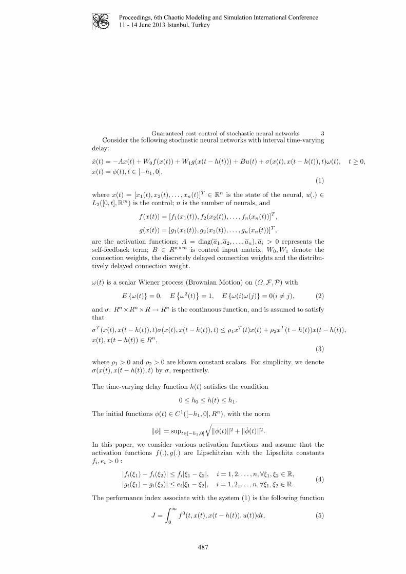
Proceedings, 6th Chaotic Modeling and Simulation International Conference
11 - 14 June 2013 Istanbul, Turkey
Guaranteed cost control of stochastic neural networks 3Consider the following stochastic neural networks with interval time-varying
delay:
x(t) = −Ax(t) + W0f(x(t)) + W1g(x(t − h(t))) + Bu(t) + σ(x(t), x(t − h(t)), t)ω(t), t ≥ 0,
x(t) = φ(t), t ∈ [−h1, 0],
(1)
where x(t) = [x1(t), x2(t), . . . , xn(t)]T ∈ Rn is the state of the neural, u(.) ∈
L2([0, t], Rm) is the control; n is the number of neurals, and
f(x(t)) = [f1(x1(t)), f2(x2(t)), . . . , fn(xn(t))]T ,
g(x(t)) = [g1(x1(t)), g2(x2(t)), . . . , gn(xn(t))]T ,
are the activation functions; A = diag(a1, a2, . . . , an), ai > 0 represents theself-feedback term; B ∈ Rn×m is control input matrix; W0,W1 denote theconnection weights, the discretely delayed connection weights and the distribu-tively delayed connection weight.
ω(t) is a scalar Wiener process (Brownian Motion) on (Ω,F ,P) with
E ω(t) = 0, E
ω2(t)
= 1, E ω(i)ω(j) = 0(i 6= j), (2)
and σ: Rn×Rn×R → Rn is the continuous function, and is assumed to satisfythat
σT (x(t), x(t − h(t)), t)σ(x(t), x(t − h(t)), t) ≤ ρ1xT (t)x(t) + ρ2x
T (t − h(t))x(t − h(t)),
x(t), x(t − h(t)) ∈ Rn,
(3)
where ρ1 > 0 and ρ2 > 0 are khown constant scalars. For simplicity, we denoteσ(x(t), x(t − h(t)), t) by σ, respectively.
The time-varying delay function h(t) satisfies the condition
0 ≤ h0 ≤ h(t) ≤ h1.
The initial functions φ(t) ∈ C1([−h1, 0], Rn), with the norm
‖φ‖ = supt∈[−h1,0]
√
‖φ(t)‖2 + ‖φ(t)‖2.
In this paper, we consider various activation functions and assume that theactivation functions f(.), g(.) are Lipschitzian with the Lipschitz constantsfi, ei > 0 :
|fi(ξ1) − fi(ξ2)| ≤ fi|ξ1 − ξ2|, i = 1, 2, . . . , n,∀ξ1, ξ2 ∈ R,
|gi(ξ1) − gi(ξ2)| ≤ ei|ξ1 − ξ2|, i = 1, 2, . . . , n,∀ξ1, ξ2 ∈ R.(4)
The performance index associate with the system (1) is the following function
J =
∫ ∞
0
f0(t, x(t), x(t − h(t)), u(t))dt, (5)
487

Proceedings, 6th Chaotic Modeling and Simulation International Conference
11 - 14 June 2013 Istanbul, Turkey
4 M. Rajchakitwhere f0(t, x(t), x(t − h(t)), u(t)) : R+ × Rn × Rn × Rm → R+, is a nonlinearcost function satisfies
∃Q1, Q2, R : f0(t, x, y, u) ≤ 〈Q1x, x〉 + 〈Q2y, y〉 + 〈Ru, u〉, (6)
for all (t, x, u) ∈ R+ × Rn × Rm and Q1, Q2 ∈ Rn×n, R ∈ Rm×m, are givensymmetric positive definite matrices. The objective of this paper is to design amemoryless state feedback controller u(t) = Kx(t) for system (1) and the costfunction (5) such that the resulting closed-loop system
x(t) = −(A−BK)x(t)+W0f(x(t))+W1g(x(t−h(t)))+σ(x(t), x(t−h(t)), t)ω(t),(7)
is mean square exponentially stable and the closed-loop value of the cost func-tion (5) is minimized.
Definition 2.1 Given α > 0. The zero solution of closed-loop system (7) isα−exponentially stabilizable in the mean square if there exist a positive numberN > 0 such that every solution x(t, φ) satisfies the following condition:
E ‖ x(t, φ) ‖ ≤ E
Ne−αt ‖ φ ‖
, ∀t ≥ 0.
Definition 2.2 Consider the control system (1). If there exist a memorylessstate feedback control law u∗(t) = Kx(t) and a positive number J∗ such thatthe zero solution of the closed-loop system (7) is mean square exponentiallystable and the cost function (5) satisfies J ≤ J∗, then the value J∗ is a guar-anteed costant and u∗(t) is a guaranteed cost control law of the system and itscorresponding cost function.
We introduce the following technical well-known propositions, which will beused in the proof of our results.
Proposition 2.1. (Integral matrix inequality [17]). For any symmetric positivedefinite matrix M > 0, scalar γ > 0 and vector function ω : [0, γ] → R
n suchthat the integrations concerned are well defined, the following inequality holds
(∫ γ
0
ω(s) ds
)T
M
(∫ γ
0
ω(s) ds
)
≤ γ
(∫ γ
0
ωT (s)Mω(s) ds
)
488

Proceedings, 6th Chaotic Modeling and Simulation International Conference
11 - 14 June 2013 Istanbul, Turkey
Guaranteed cost control of stochastic neural networks 53 Design of guaranteed cost controller
In this section, we give a design of memoryless guaranteed feedback cost controlfor stochastic neural networks (1). Let us set
W11 = −AP − PAT − 2αP − BBT + 0.25BRBT +
1∑
i=0
Gi −
1∑
i=0
e−2αhiHi
+ 4PFD−10 FP + PQ1P + 2ρ1PP,
W12 = P + AP + 0.5BBT ,
W13 = e−2αh0H0 + 0.5BBT + AP,
W14 = 2e−2αh1H1 + 0.5BBT + AP,
W15 = P0.5BBT + AP,
W22 =
1∑
i=0
WiDiWTi +
1∑
i=0
h2i Hi + (h1 − h0)U − 2P − BBT ,
W23 = P, W24 = P, W25 = P,
W33 = −e−2αh0G0 − e−2αh0H0 − e−2αh1U +
1∑
i=0
WiDiWTi ,
W34 = 0, W35 = e−2αh1U,
W44 =1
∑
i=0
WiDiWTi − e−2αh1U − e−2αh1G1 − e−2αh1H1, W45 = e−2αh1U,
W55 = −e−2αh1U +
1∑
i=0
WiDiWTi − e−2αh2U + 4PED−1
1 EP + PQ2P + 2ρ2PP,
E = diagei, i = 1, . . . , n, F = diagfi, i = 1, . . . , n,
λ1 = λmin(P−1),
λ2 = λmax(P−1) + h0λmax[P
−1(
1∑
i=0
Gi)P−1]
+ h21λmax[P
−1(
1∑
i=0
Hi)P−1] + (h1 − h0)λmax(P
−1UP−1).
Theorem 3.1. Consider control system (1) and the cost function (5). If thereexist symmetric positive definite matrices P,U,G0, G1,H0,H1, and diagonalpositive definite matrices Di, i = 0, 1 satisfying the following LMIs
W11 W12 W13 W14 W15
∗ W22 W23 W24 W25
∗ ∗ W33 W34 W35
∗ ∗ ∗ W44 W45
∗ ∗ ∗ ∗ W55
< 0, (8)
489

Proceedings, 6th Chaotic Modeling and Simulation International Conference
11 - 14 June 2013 Istanbul, Turkey
6 M. Rajchakitthen
u(t) = −1
2BT P−1x(t), t ≥ 0. (9)
is a guaranteed cost control and the guaranteed cost value is given by
J∗ = E
λ2‖φ‖2
.
Moreover, the solution x(t, φ) of the system satisfies
E ‖ x(t, φ) ‖ ≤ E
√
λ2
λ1e−αt ‖ φ ‖
, ∀t ≥ 0.
Proof. Let Y = P−1, y(t) = Y x(t). Using the feddback control (7) we considerthe following Lyapunov-Krasovskii functional and taking the mathematical ex-pectation
E V (t, xt) = E
6∑
i=1
Vi(t, xt)
,
E V1 = E
xT (t)Y x(t)
,
E V2 = E
∫ t
t−h0
e2α(s−t)xT (s)Y G0Y x(s) ds
,
E V3 = E
∫ t
t−h1
e2α(s−t)xT (s)Y G1Y x(s) ds
,
E V4 = E
h0
∫ 0
−h0
∫ t
t+s
e2α(τ−t)xT (τ)Y H0Y x(τ) dτ ds
,
E V5 = E
h1
∫ 0
−h1
∫ t
t+s
e2α(τ−t)xT (τ)Y H1Y x(τ) dτ ds
,
E V6 = E
(h1 − h0)
∫ t−h0
t−h1
∫ t
t+s
e2α(τ−t)xT (τ)Y UY x(τ) dτ ds
.
It easy to check that
E
λ1 ‖ x(t) ‖2
≤ E V (t, xt) ≤ E
λ2 ‖ xt ‖2
, ∀t ≥ 0, (10)
490

Proceedings, 6th Chaotic Modeling and Simulation International Conference
11 - 14 June 2013 Istanbul, Turkey
Guaranteed cost control of stochastic neural networks 7Taking the derivative of Vi, i = 1, 2, . . . , 6 and taking the mathematical expec-tation, we have
E
V1
=E
2xT (t)Y x(t)
=E
yT (t)[−PAT − AP ]y(t) − yT (t)BBT y(t)
+ E
2yT (t)W0f(.) + 2yT (t)W1g(.) + 2yT (t)σω(t)
;
E
V2
=E
E
yT (t)G0y(t) − e−2αh0yT (t − h0)G0y(t − h0) − 2αV2
;
E
V3
=E
yT (t)G1y(t) − e−2αh1yT (t − h1)G1y(t − h1) − 2αV3
;
E
V4
=E
h20y
T (t)H0y(t) − h1e−2αh0
∫ t
t−h0
xT (s)H0x(s) ds − 2αV4
;
E
V5
=E
h21y
T (t)H1y(t) − h1e−2αh1
∫ t
t−h1
yT (s)H1y(s) ds − 2αV4
;
E
V6
=E
(h1 − h0)2yT (t)Uy(t) − (h1 − h0)e
−2αh1
∫ t−h0
t−h1
yT (s)Uy(s) ds − 2αV6
.
Applying Proposition 2.1 and the Leibniz - Newton formula∫ t
s
y(τ)dτ = y(t) − y(s),
we have for i, j = 0, 1, :
−E
hi
∫ t
t−hi
yT (s)Hj y(s) ds
≤ −E
[∫ t
t−hi
y(s) ds
]T
Hj
[∫ t
t−hi
y(s) ds
]
≤ −E
[y(t) − y(t − h(t))]T Hj [y(t) − y(t − h(t))]
= −E
yT (t)Hjy(t) + 2xT (t)Hjy(t − h(t))
− E
yT (t − hi)Hjy(t − hi)
.
(11)
Note that
E
∫ t−h0
t−h1
yT (s)Uy(s) ds
= E
∫ t−h(t)
t−h1
yT (s)Uy(s) ds
+E
∫ t−h0
t−h(t)
yT (s)Uy(s) ds
.
Applying Proposition 2.1 gives
E
[h1 − h(t)]
∫ t−h(t)
t−h1
yT (s)Uy(s)ds
≥ E
[
∫ t−h(t)
t−h1
y(s)ds]T
U[
∫ t−h(t)
t−h1
y(s)ds]
≥ E
[y(t − h(t) − y(t − h1)]T U [y(t − h(t) − y(t − h1)]
.
Since h1 − h(t) ≤ h1 − h0, we have
E
[h1 − h0]
∫ t−h(t)
t−h1
yT (s)Uy(s)ds
≥ E
[y(t − h(t) − y(t − h1)]T U [y(t − h(t) − y(t − h1)]
,
491

Proceedings, 6th Chaotic Modeling and Simulation International Conference
11 - 14 June 2013 Istanbul, Turkey
8 M. Rajchakitthen
−E
[h1 − h0]
∫ t−h(t)
t−h1
yT (s)Uy(s)ds
≤ −E
[y(t − h(t) − y(t − h1)]T U [y(t − h(t) − y(t − h1)]
.
Similarly, we have
−E
(h1 − h0)
∫ t−h0
t−h(t)
yT (s)Uy(s) ds
≤ −E
[y(t − h0) − y(t − h(t))]T U [y(t − h0) − y(t − h(t)]
.
Then, we have
E
V (.) + 2αV (.)
≤ E
yT (t)[−PAT − AP ]y(t) − yT (t)BBT y(t) + 2yT (t)W0f(.)
+ E
2yT (t)W1g(.) + 2yT (t)σω(t) + yT (t)(
1∑
i=0
Gi)y(t) + 2α〈Py(t), y(t)〉
+ E
yT (t)(1
∑
i=0
h2i Hi)y(t) + (h1 − h0)y
T (t)Uy(t)
− E
1∑
i=0
e−2αhiyT (t − hi)Giy(t − hi)
− E
e−2αh0 [y(t) − y(t − h0)]T H0[y(t) − y(t − h0)]
− E
e−2αh1 [y(t) − y(t − h1)]T H1[y(t) − y(t − h1)]
− E
e−2αh1 [y(t − h(t)) − y(t − h1)]T U [y(t − h(t)) − y(t − h1)]
− E
e−2αh1 [y(t − h0) − y(t − h(t))]T U [y(t − h0) − y(t − h(t))]
.
(12)
Using the equation (7)
P y(t) + APy(t) − W0f(.) − W1g(.) + 0.5BBT y(t) − σω(t) = 0,
and multiplying both sides with [2y(t),−2y(t), 2y(t − h0), 2y(t − h1), 2y(t −h(t)), 2σω(t)]T , and taking the mathematical expectation, we have
E
2yT (t)P y(t) + 2yT (t)APy(t) − 2yT (t)W0f(.) − 2yT (t)W1g(.)
+ E
yT (t)BBT y(t) − 2yT (t)σω(t)
= 0,
− E
2yT (t)P y(t) − 2yT (t)APy(t) + 2yT (t)W0f(.)
+ E
2yT (t)W1g(.) − yT (t)BBT y(t) + 2yT (t)σω(t)
= 0,
E
2yT (t − h0)P y(t) + 2yT (t − h0)APy(t) − 2yT (t − h0)W0f(.)
− E
2yT (t − h0)W1g(.) + yT (t − h0)BBT y(t) − 2yT (t − h0)σω(t)
= 0,
E
2yT (t − h1)P y(t) + 2yT (t − h1)APy(t) − 2yT (t − h1)W0f(.)
− E
2yT (t − h1)W1g(.) + yT (t − h1)BBT y(t) − 2yT (t − h1)σω(t)
= 0,
492

Proceedings, 6th Chaotic Modeling and Simulation International Conference
11 - 14 June 2013 Istanbul, Turkey
Guaranteed cost control of stochastic neural networks 9E
2yT (t − h(t))P y(t) + 2yT (t − h(t))APy(t) − 2yT (t − h(t))W0f(.)
− E
2yT (t − h(t))W1g(.) + yT (t − h(t))BBT y(t) − 2yT (t − h(t))σω(t)
= 0,
E
2ωT (t)σT P y(t) + 2ωT (t)σT APy(t) − 2ωT (t)σT W0f(.)
− E
2ωT (t)σT W1g(.) + ωT (t)σT BBT y(t) − 2ωT (t)σT σω(t)
= 0.
(13)
Adding all the zero items of (13) and f0(t, x(t), x(t−h(t)), u(t))−f0(t, x(t), x(t−h(t)), u(t)) = 0, respectively into (12), applying asumption (2), (3), using thecondition (6) for the following estimations and taking the mathematical expec-tation
E
f0(t, x(t), x(t − h(t)), u(t))
≤E 〈Q1x(t), x(t)〉 + 〈Q2x(t − h(t)), x(t − h(t))〉
+ E 〈Ru(t), u(t)〉
=E 〈PQ1Py(t), y(t)〉 + 〈PQ2Py(t − h(t)), y(t − h(t))〉
+ E
0.25〈BRBT y(t), y(t)〉
,
E 2〈W0f(x), y〉 ≤E
〈W0D0WT0 y, y〉 + 〈D−1
0 f(x), f(x)〉
,
E 2〈W1g(z), y〉 ≤E
〈W1D1WT1 y, y〉 + 〈D−1
1 g(z), g(z)〉
,
E
2〈D−10 f(x), f(x)〉
≤E
〈FD−10 Fx, x〉
,
E
2〈D−11 g(z), g(z)〉
≤E
〈ED−11 Ez, z〉
,
we obtain
E
V (.) + 2αV (.)
≤E
ζT (t)Eζ(t) − f0(t, x(t), x(t − h(t)), u(t))
, (14)
where ζ(t) = [y(t), y(t), y(t − h0), y(t − h1), y(t − h(t))], and
E =
W11 W12 W13 W14 W15
∗ W22 W23 W24 W25
∗ ∗ W33 W34 W35
∗ ∗ ∗ W44 W45
∗ ∗ ∗ ∗ W55
.
Therefore, by condition (8), we obtain from (14) that
E
V (t, xt)
≤ −E 2αV (t, xt) , ∀t ≥ 0. (15)
Integrating both sides of (15) from 0 to t, we obtain
E V (t, xt) ≤ E
V (φ)e−2αt
, ∀t ≥ 0.
Furthermore, taking condition (10) into account, we have
E
λ1 ‖ x(t, φ) ‖2
≤ E V (xt) ≤ E
V (φ)e−2αt
≤ E
λ2e−2αt ‖ φ ‖2
,
then
E ‖ x(t, φ) ‖ ≤ E
√
λ2
λ1e−αt ‖ φ ‖
, t ≥ 0,
493

Proceedings, 6th Chaotic Modeling and Simulation International Conference
11 - 14 June 2013 Istanbul, Turkey
10 M. Rajchakitwhich concludes the mean square exponential stability of the closed-loop system(2.7). To prove the optimal level of the cost function (5), we derive from (14)and (8) that
E
V (t, zt)
≤ −E
f0(t, x(t), x(t − h(t)), u(t))
, t ≥ 0. (16)
Integrating both sides of (18) from 0 to t leads to
E
∫ t
0
f0(t, x(t), x(t − h(t)), u(t))dt
≤ E V (0, z0) − V (t, zt) ≤ E V (0, z0) ,
dute to E V (t, zt) ≥ 0. Hence, letting t → +∞, we have
J = E
∫ ∞
0
f0(t, x(t), x(t − h(t)), u(t))dt
≤ E V (0, z0) ≤ E
λ2‖φ‖2
= J∗.
This completes the proof of the theorem.
Example 3.1. Consider the stochastic neural networks with interval time-varying delays (2.1), where
A =
[
0.2 00 0.2
]
,W0 =
[
−0.3 0.10.1 −0.3
]
,W1 =
[
−0.4 0.30.3 −0.9
]
, B =
[
0.50.4
]
,
E =
[
0.7 00 0.9
]
, F =
[
0.7 00 0.8
]
, Q1 =
[
0.7 0.20.2 0.6
]
, Q2 =
[
0.2 0.30.3 0.3
]
, R =
[
0.9 0.50.5 0.8
]
,
h(t) = 0.1 + 2.0297 sin2 t if t ∈ I = ∪k≥0[2kπ, (2k + 1)π]
h(t) = 0 if t ∈ R+ \ I,
Note that h(t) is non-differentiable, therefore, the stability criteria proposed in[5, 6, 7, 12, 15] are not applicable to this system. Given α = 1.1, ρ1 = 0.5, ρ1 =0.8, h0 = 0.1, h1 = 2.1297, by using the Matlab LMI toolbox, we can solve forP,U,G0, G1,H0,H1,D0, and D1 which satisfy the condition (3.1) in Theorem3.1. A set of solutions are
P =
[
3.1297 0.48310.4831 1.1970
]
, U =
[
2.0912 0.12910.1291 3.0017
]
,
G0 =
[
0.1473 0.01130.0113 0.8931
]
, G1 =
[
0.6179 0.11970.1197 1.0273
]
,
H0 =
[
1.0387 0.39700.3970 2.2207
]
, H1 =
[
0.9712 0.00120.0012 0.7219
]
,
D0 =
[
0.2189 00 0.2189
]
, D1 =
[
0.1249 00 0.1249
]
.
Thenu(t) = −1.7196x1(t) − 1.2551x2(t), t ≥ 0
494

Proceedings, 6th Chaotic Modeling and Simulation International Conference
11 - 14 June 2013 Istanbul, Turkey
Guaranteed cost control of stochastic neural networks 11
is a guaranteed cost control law and the cost given by
J∗ = E
11.3271 ‖φ‖2
.
Moreover, the solution x(t, φ) of the system satisfies
E ‖x(t, φ)‖ ≤ E
0.7315e−1.1t ‖φ‖
,∀t ≥ 0.
4 Conclusions
In this paper, the problem of guaranteed cost control for stochastic neuralnetworks with interval nondifferentiable time-varying delay has been studied.A nonlinear quadratic cost function is considered as a performance measure forthe closed-loop system. The stabilizing controllers to be designed must satisfysome mean square exponential stability constraints on the closed-loop poles. Byconstructing a set of time-varying Lyapunov-Krasovskii functional combinedwith Newton-Leibniz formula, a memoryless state feedback guaranteed costcontroller design has been presented and sufficient conditions for the existenceof the guaranteed cost state-feedback for the system have been derived in termsof LMIs.
Acknowledgements. This work was supported by the Thai Research FundGrant, the Higher Education Commission and Faculty of Science, Maejo Uni-versity, Thailand.
References
1.Hopfield J.J., “Neural networks and physical systems with emergent collective com-putational abilities,” Proc. Natl. Acad. Sci. USA, 79(1982), 2554-2558.
2.Kevin G., An Introduction to Neural Networks, CRC Press, 1997.3.Wu M., He Y., She J.H., Stability Analysis and Robust Control of Time-Delay
Systems, Springer, 2010.4.Arik S., An improved global stability result for delayed cellular neural networks,
IEEE Trans. Circ. Syst. 499(2002), 1211-1218.5.He Y., Wang Q.G., M. Wu, LMI-based stability criteria for neural networks with
multiple time-varying delays, Physica D, 112(2005), 126-131.6.Kwon O.M., J.H. Park, Exponential stability analysis for uncertain neural networks
with interval time-varying delays. Appl. Math. Comput., 212(2009), 530541.7.Phat V.N., Trinh H. , Exponential stabilization of neural networks with various ac-
tivation functions and mixed time-varying delays, IEEE Trans. Neural Networks,
21(2010), 1180-1185.8.Botmart T.and P. Niamsup, Robust exponential stability and stabilizability of linear
parameter dependent systems with delays, Appl. Math. Comput., 217(2010),2551-2566.
9.W.H. Chen W.H., Guan Z.H., Lua X., Delay-dependent output feedback guaranteedcost control for uncertain time-delay systems, Automatica, 40(2004), 1263 - 1268.
495

Proceedings, 6th Chaotic Modeling and Simulation International Conference
11 - 14 June 2013 Istanbul, Turkey
12 M. Rajchakit10.Palarkci M.N., Robust delay-dependent guaranteed cost controller design for un-
certain neutral systems,Appl. Math. Computations, 215(2009), 2939-2946.11.Park J.H., Kwon O.M., On guaranteed cost control of neutral systems by retarded
integral state feedback, Applied Mathematics and Computation, 165(2005), 393-404.
12.Park J.H., Choi K., Guaranteed cost control of nonlinear neutral systems viamemory state feedback, Chaos, Fractals and Solitons, 24(2005), 183-190.
13.Fridman E., Orlov Y., Exponential stability of linear distributed parameter systemswith time-varying delays. Automatica, 45(2009), 194201.
14.Xu S., Lam J., A survey of linear matrix inequality techniques in stability analysisof delay systems. Int. J. Syst. Sci., 39(2008), 12, 10951113.
15.Xie J.S., Fan B.Q., Young S.L., Yang J., Guaranteed cost controller design ofnetworked control systems with state delay, Acta Automatica Sinica, 33(2007),170-174.
16.Yu L., Gao F., Optimal guaranteed cost control of discrete-time uncertain systemswith both state and input delays, Journal of the Franklin Institute, 338(2001),101-110.
17.Gu K., Kharitonov V., Chen J., Stability of Time-delay Systems, Birkhauser,Berlin, 2003.
496
Proceedings, 6th Chaotic Modeling and Simulation International Conference
11 - 14 June 2013 Istanbul, Turkey
Two-Side Confidence Intervals for the Poisson Means
Manlika Rajchakit Major of Statistics, Faculty of Science, Maejo University, Chiang Mai 50290,
Thailand.
E-mail: [email protected].
Abstract: In this paper we consider interval estimation for the Poisson means. The
following confidence intervals are considered: Wald CI, Score CI, Score continuity
correction CI, Agresti and Coull CI, Bayes Wald CI, Bayes Score CI, and Bayes Score
continuity correction CI. Each interval is examined for its coverage probability and its
expected lengths. Based on this simulation; we recommend Score CI and the Wald CI for
the small n and the larger n respectively.
Keywords: Bayes Estimators; Poisson distribution; Interval Estimation.
1. Introduction
Estimation is one of the main branches of statistics. They refer to the process
by which one makes inference about a population, based on information
obtained from a sample. Statisticians use sample statistics to estimate
population parameter. For example; sample means are used to estimate
population mean; sample proportions, and to estimate proportions. An estimate
of population parameters may be expressed in two ways; point and interval
estimate. A point estimate of a population parameter is a single value of a
statistic, for example, the sample mean x is a point estimate of the population
meanµ . Similarly, the sample proportion p is a point estimate of the population
proportion P. An interval estimate is defined by two numbers, between which a
population parameter is to lie, for example, a x b< < is an interval estimate of
the population meanµ . It indicates that the population mean is greater than a
bit less than b. Statisticians use a confidence interval to express the precision
and uncertainty associated with a particular sampling method, for example, we
might say that we are 95% confidence that the true population mean falls
within a specified range. This statement is a confidence interval. It mean that if
we used the same sampling method to select different samples and compute
different interval estimates, the true population mean would fall within a range
defined by the sample statistic ± margin of error 95% of the time.
In this paper, we are compare seven method confidence interval (CIs) for the
Poisson means, Poisson distribution is a discrete probability distribution. A
Poisson random variable (X) representing the number of successes occurring in
a given time interval or a specified region of space.
The probability distribution is
( )xe
P Xx!
−λλ= .
497

Proceedings, 6th Chaotic Modeling and Simulation International Conference
11 - 14 June 2013 Istanbul, Turkey
Where x=0, 1, 2,…, e=2.71828 (but use your calculator’s e button), and
λ =mean number of successes in the given time interval or region of space.
Confidence interval (CI) of Poisson means that popular is
2
ˆ ˆz n ,αλ ± λ
and 2zα is the ( )100 1 2−α percentile of the standard normal distribution.
This formula, we call Wald method, it is easy to present and compute but it has
poor coverage properties for small n. Brown, Cai and das Gupta [2] showed
that Wald CI is actually far too poor and unreliable and the problem are not just
for small n. Cai [1] showed that Wald CI suffers from a series systematic bias
in the coverage. Therefore, the other researcher are present any method for
solve this problem; see Manlika [3], Ross [4], Stamey [5] and Wardell [7]. We
have known that common method used maximum likelihood estimator. So, we
require to developed the CIs by Bayes estimator with Wald CI, Score CI and
Score continuity correction CI which the prior distribution of λ is assumed to
be gamma distribution with α and β parameters. Wararit [6] showed that the
optimal values of α and β are their value provide αβ closed to the λ
parameter. The α value is always higher than the β value, the α lies between
4.0 and 5.0.
2. The confidence interval
1. Create random variable that has Poisson
distribution.
2. Compute interval estimation for a Poisson
distribution seven methods:
2.1 Wald CI
ˆˆ Z
n
λλ ± . (a)
2.2 Score CI
( )2 1 22
1 2
ˆn z 2 zˆznn 4n
−λ +
± λ +
. (b)
498

Proceedings, 6th Chaotic Modeling and Simulation International Conference
11 - 14 June 2013 Istanbul, Turkey
2.3 Score continuity correction CI
( )2 2ˆ ˆ2n Z 1 Z Z 4n 2
2n
λ + − + λm m. (c)
2.4 Agresti and Coull CI
2 21 2X z 2 X z 2
z nn n
− + +±
. (d)
2.5 Bayes Wald CI
Zn
λλ ±
%% . (e)
2.6 Bayes Score CI
( ) 1 22
21 2
n z 2 zzn
n 4n
−λ +
± λ +
%%%%
% %.
(f)
2.7 Bayes Score continuity correction CI
( )2 22n Z 1 Z Z 4n 2
2n
λ + − + λ% %% %m m
%. (g)
Note that for (a)-(c) ˆ xλ = ; λ is well known to be the MLE of λ and z is the
( )100 1 2−α percentile of the standard normal distribution
For (e)-(g) ( )X
n 1
α + βλ =
β+% and n n 1= β+% .
λ% is Bayes’ estimator of Poisson mean, and
X is number of successes occurring in a given time interval
or a specified region of space.
3. Simulation results The performance of the estimated coverage probabilities of the confidence
interval (a)-(f) and their expected lengths were examined via Monte Carlo
simulation. Data were generate from Poisson distribution with 1,2,3,4,5λ = and
sample size n=10 to 100. All simulations were performed using programs
499

Proceedings, 6th Chaotic Modeling and Simulation International Conference
11 - 14 June 2013 Istanbul, Turkey
written in the R Statistical software, repeated 1,000 times in each case at level of
significance 0.01,0.05,α = and 0.10. The simulation results are shown in Figure
1-2 and Table 1.
Figure 1 show that the coverage probability of the Wald CI, Score CI, Agresti
and Coull CI, and Score continuity correction CI for fixed 3λ = and variable n
from 10 to 100. Naively, are may expect that the coverage probability gets
systematically near the nominal level as the sample size n increases.
Wald CI Score CI
Agresti and Coull CI Score continuity correction CI
Figure1 Coverage probability of four intervals for a Poisson mean with
0.05α = and n 10= to 100.
Figure2. Show that the coverage probability of the alternative intervals with
Bayes estimator gives the coverage probability upper nominal level.
500

Proceedings, 6th Chaotic Modeling and Simulation International Conference
11 - 14 June 2013 Istanbul, Turkey
Bayes Wald CI Bayes Score CI
Bayes Score continuity correction CI
Figure2 Coverage probability of three intervals for a Poisson mean with
0.05α = and n 10= to 100.
In addition, the expected lengths of the score CI and the Wald CI are much
shorter than the other CIs when n are small and larger respectively. The
expected length increase as the value λ gets larger (e.g. For Score CI, n=10
and 0.05α = ; 0.23284 for 1λ = ; 0.327333 for 3λ = ; and 0.482786 for 5λ = ).
Moreover, when the sample size increase, the expected length is shorter (e.g.
For Score CI, 1λ = and; 0.23284 for n=10; 0.102252 for n=50; and 0.072279
for n=100).
4. Conclusions
Our main objective is to compare the CIs under different situation; we compare
the performance of all the CIs described above under various situations and
three different confidence levels 0.05,0.01,0.10α = . We found that, Wald CI is
below the nominal level, but it has smallest expected length for n are small
(n<30), Score CI , Score corrected continuity CI , Agresti and Coull CI are
above the nominal level and they have expected length slightly higher Wald CI.
Three alternatives with Bayes estimator have a higher CI and they are similar
with each other and do a good job, so, we recommend Score CI and the Wald CI
for the small n and the larger n respectively.
References [1] T. T. Cai, “One-sided confidence intervals in discrete distributions”, J. of Statistical planning
and inference, 131 (2005) 63-88.
[2] D. B. Lawrence, T. T. Cai, and A. Dasgupta, “Interval estimation for a binomial Proportion”, Statistica Sinica, 16 (2003):101-133.
[3] M. Tanusit, “A Comparative Study of Parameter Inference Methods for Poisson distribution:
Small Sample Size”, Advance and Applications in Statistics, 14 (2010):49-55. [4] T. D. Ross, “Accurate confidence intervals for binomial proportion and Poisson rate
estimation”, Comput. Biol. Med, 33 (2003) : 509-531.
501

Proceedings, 6th Chaotic Modeling and Simulation International Conference
11 - 14 June 2013 Istanbul, Turkey
[5] J. D. Stamey, J. W. Seaman, and D. M. Young, “Bayesian analysis of complementary Poisson rate parameters with data subject to misclassification”, Statist. Plann. Inference, 134 (2005),
36-48.
[6] W. Panichkitkosolkul, “The Optimal Parameters of Prior Distribution for Bayes’ Estimator of Poisson Mean”, SWU Sci. J., 23 No. 1 (2007) 23-31.
[7] G. D. Wardell, “Small Sample Interval Estimation of Bernoulli and Poisson Parameters”, The
American Statistician, 51 (1997) : 321-325
Manlika Tanusit received the B.S. degree in Statistics from Kasetsart University, Bangkok City, Thailand, in 2008. Currently, she is a lecturer at
the Department of Statistics, Maejo University, Chiang Mai, Thailand. His
research interests include stability and stabilization of dynamical systems, qualitative theory of differential/discrete-time systems.
Email: [email protected]
502

Proceedings, 6th Chaotic Modeling and Simulation International Conference
11 - 14 June 2013 Istanbul, Turkey
Correlation and Randomness Properties of Binary
Sequences Generated Using Matrix Reccurence
Relation Defined over Z8
Ramesh S*, Dileep D
#
*Department of Electronics & Communication Engineering,
Dr Ambedkar Institute of Technology, Bangalore, India #Istrac, ISRO, Bangalore
E-mail: [email protected]
Abstract: This article describes an approach to the generation of key sequence based on
matrix recurrence relation defined over Z8. The generated sequence is subjected to FIPS
140-1 test suite and Hamming Autocorrelation test .The generated sequence passes the
FIPS 140-1 test suite and also exhibits good Hamming autocorrelation properties. The
results of these tests are analyzed.
Keywords: Random number, pseuodo random number, Recurrence relation over Z8,
Auto correlation
1. Introduction
Good Cryptography requires good random numbers. Security of
these protocols relies on the unpredictability of the key they use.
Almost all cryptographic protocols require the generation and use
of secret value that must be unknown to attacker. Random number
generators used to generate key sequence must satisfy stringent
requirements like unpredictability, uniform distribution, long
period, and good statistical properties. Pierrie L’Ecuyer[1,2,3,4
]discusses the most widely used random number generators based
on linear recurrence models such as Multiple recurrence
generators, Multiple recurrence generators with carry ,the Linear
feedback shift registers etc.., The authors proposed the [ 5,6,7]
random number generator based on the matrix recurrence relation
defined over Z8 . In this paper the generation of sequence of
random number defined over z8 based on matrix recurrence
relation, the FIPS 140-1 tests performed on the proposed generator
and the Hamming auto correlation properties of the sequence so
generated are also discussed.
503

Proceedings, 6th Chaotic Modeling and Simulation International Conference
11 - 14 June 2013 Istanbul, Turkey
2. Organization of the paper
The rest of this article is organized as follow. In Section II, we
present a proposed a random number generator defined over Z8
using matrix recurrence relation. In Section III, we discuss briefly
the FIPS 140-1 tests and Normalized Hamming autocorrelation
test, which are used to test the proposed random number generator.
3. The Proposed Random Number Generator defined over Z8
Based on matrix recurrence relation [5, 6]
The following matrix recurrence relation defines the proposed
random number generator over Z8 [5, 6, and 7]
X j =1
1
0
ij
k
i
i XC
, j ≥ k+1 arithmetic modulo 8 (1)
Where X is an n-tuple (nx1) over Z8 and coefficients
Ci , i = 0 to k-1and can be
a) n x n non-singular matrix over Z8 or
b) Any n x n arbitrary matrix over Z8
When m is prime X is a vector otherwise it is an element of
module over Z8.
Output is concatenated sequence xi T where xi
T is transpose of
xi, i =0,1,2,……
4. Testing of Random Numbers
The evaluations of the quality of the random number generators
are very difficulty problem, which has no unique solution. On the
other hand there is no single practical tests that can realize the
randomness in a given sequence of random numbers. Since all the
504

Proceedings, 6th Chaotic Modeling and Simulation International Conference
11 - 14 June 2013 Istanbul, Turkey
pseudorandom sequence generators are based on deterministic
rules, there exist always tests in which a given generator will fail.
A large number of statistical tests have been proposed, such as
DIEHARD specification FIPS 140-1 and Knuth’s test,
Autocorrelation test, Crypt -XS. In this paper we compute the
FIPS 140-1 test statistics for a binary sequence generated by the
equation (1) and also the autocorrelation test is performed on the
sequence generated by the equation (1).
The Frequency test, serial test (two-bit test), Poker test, runs test,
autocorrelation test are the five statistical tests that are commonly
used for determining whether the binary sequence s possesses
some specific characteristics that a truly random sequence would
be likely to exhibit [5]. These tests are discussed in detail in papers
[Knuth] [Menezes] [5, 6, 11, and 12]
4.1. FIPS 140-1 Statistical Tests for Randomness
The second and following pages should begin 1.0 inch (2.54 cm)
from the top edge. On all pages, the bottom margin should be 1-
1/8 inches (2.86 cm) from the bottom edge of the page for 8.5 x
11-inch paper; for A4 paper, approximately 1-5/8 inches (4.13 cm)
from the bottom edge of the page.
Federal Information Processing Standard FIPS- 140-1 specifies
monobit test. Poker test runs test and long run test for computing
the statistics for randomness also provide the explicit bounds that
the computed value of a statistic must satisfy. A single bit string s
of length 20000 bits, output from a generator, is subjected to each
of the above tests. If any of the tests fail, then the generator fails
the test.[ 5,6,7,8, 12].
4.1.1. Monobit test
The number n1 of 1’s in sequence s should satisfy 9654 < n1<
10346.
4.1.2. Poker test
Let q be a positive integer such that n/q ≥5. (2q), and let k =
n/q . Divide the sequence s into k non-overlapping parts each of
505

Proceedings, 6th Chaotic Modeling and Simulation International Conference
11 - 14 June 2013 Istanbul, Turkey
length q, and let ni be the number of occurrences of the ith
type of
sequence of length q, 1 ≤ i ≥ 2q.
X2=2q/k
kn
q
i
i
2
1
2
2
The statistic X2 defined by equation (2) is computed for m = 4.
The poker test is passed if 1.03 < X2 < 57.4.
4.1.3. Runs test
The number Bi and Gi of blocks and gaps, respectively, of
length i in sequence s are counted for each i, 1 ≤ i ≤ 6. (For the
purpose of this test, runs of length greater than 6 are considered to
be of length 6.) The runs test is passed if the 12 counts Bi and Gi, 1
≤ i ≤ 6, are each within the corresponding interval specified by the
table 1
Table 1.Interval specified for Run test
Length
of run
Required interval
1 2267 − 2733
2 1079 − 1421
3 502 − 748
4 223 − 402
5 90 − 223
6 90 − 223
4.1.4. Long run test
The long run test is passed if there are no runs of length 34 or
more. FIPS 140-1 allows these tests to be substituted by alternative
tests, which provide equivalent or superior randomness checking.
4.2. Hamming Auto Correlation Test
One of the desirable properties of sequence of random numbers is
that, the elements of the sequence must not be clustered [5-7, 12].
506

Proceedings, 6th Chaotic Modeling and Simulation International Conference
11 - 14 June 2013 Istanbul, Turkey
This property can be verified by computing normalized Hamming
correlation of the sequence Rh(τ) which is given by equation (3).
Rh(τ) = (a-d)/(a+d) (3)
Where a = agreements, d = disagreements between bits of
sequence and its shifted version and τ is time shift. Rh (τ)) is
computed by counting the number of agreements and
disagreements for different time shifts. The value of Rh(τ) ranges
between +1 and –1. For τ =0, Rh(τ) =1,since there is no
disagreements.
Table 2. Matrix used for computing recurrence equationrence
equation (1)
C0 C1 C2 C3 C4
7 0
0 1
5 0
1 1
6 1
1 1
3 1
1 2
5 2
1 1
C5 C6 C7 C8 C9
3 3
3 4
4 3
3 5
7 5
1 2
5 4
1 3
0 7
1 5
C10 C11 C12 C13 C14
3 4
5 7
6 5
1 3
4 5
1 3
5 7
1 4
1 4
1 7
C15 C16 C17 C18 C19
2 1
1 1
3 2
1 1
6 3
1 1
7 1
4 1
5 5
3 2
Table 3 .Initial vectors used for computing recurrence equation (1)
X1 X2 X3 X4 X5 X6 X7
1
2
3
1
4
5
6
1
3
7
5
1
7
0
X8 X9 X1
0
X1
1
X12 X13 X14
5
2
5
4
3
2
2
3
7
3
1
3
4
4
X1
5
X1
6
X1
7
X1
8
X19 X20
3
3
5
0
1
5
6
2
5
6
4
6
507

Proceedings, 6th Chaotic Modeling and Simulation International Conference
11 - 14 June 2013 Istanbul, Turkey
5 Results and discussion
5.1. FIPS-140-1 Tests Results
The sequence of length 20000 consecutive binary mapped bits
generated using equation (1) is subjected to FIPS 140-1 statistical
test to determine the randomness property. Table 2 gives an array
of 20 arbitrary 2 x 2 matrix over Z8 and the sequence is generated
by using these matrices as co efficient matrix in the equation (1)
for different stages k = 3 to 20.Table 3 gives corresponding initial
vectors used for the generation of the sequence. The results are
tabulated in Table 4 for different stages k = 3 to 20.
Results show that, the sequences passes FIPS 140-1 tests for stages
k > 4 for the given matrices and initial vector. However for the
stages k ≤ 4 the sequence doesn’t pass all the tests but few. The
algorithm is tested for different sets of 2 x 2 matrices
Table 4. Results of FIPS 140-1 tests carried out on the recurrence
equation (1)
Rando
mness
test
Case 1
3 stages
Case 2
4 stages
Mono
bit Test
n1 n0 n1 n0
1022
0
9798 9992 1000
8
Poker
Test
265.88 171.75
Run
Test
Run
1
Run
0
Run
1
Run
0
1 2259 2420 2384 2400
2 1395 1399 1311 1274
3 564 537 701 693
4 377 322 278 286
5 216 162 134 190
6 135 102 166 130
Long
run test
Passes Long run test
508

Proceedings, 6th Chaotic Modeling and Simulation International Conference
11 - 14 June 2013 Istanbul, Turkey
Rando
mness
test
Case 3
5 stages
Case 4
6 stages
Mono-
bit Test
n1 n0 n1 n1
9988 1001
2
9930 9988
Poker
Test
7.6544 12.768
Run
Test
Run
1
Run
0
Run
Test
Run
1
1 2500 2433 1 2500
2 1214 1273 2 1214
3 627 662 3 627
4 311 299 4 311
5 168 161 5 168
6 159 151 6 159
Long
run test
Passes Long run test
and initial vectors and it is found that for k > 4 the sequence
generated pass FIPS 140-1 tests.
5.2 Hamming Autocorrelation Test Results
Sequence xi T is over Z8 and is converted into a binary
sequence where 0,1,2,3,4,5,6,7 are replaced by binary 3-tuples
000,001,010,011,100,101,110, 111 respectively.
Hamming correlation Rh(τ) is computed using equation (3) by
considering
i) Sequence of 10,000 consecutive output integer of the recurrence
equation (1) which is right circularly shifted by τ shifts, τ =
0,1,…., 9999,and
ii) Sequence of 20,000 consecutive output bits of the recurrence
equation (1) which is right circularly shifted by τ shifts, τ =
0,1,…., 19999
509

Proceedings, 6th Chaotic Modeling and Simulation International Conference
11 - 14 June 2013 Istanbul, Turkey
Plots of Normalized Hamming autocorrelation test are shown in
Figure 1 to 6
Rando
mness
test
Case 5
7 stages
Case 6
8 stages
Mono
bit Test
n1 n0 n1 n0
9887 1011
3
991
8
10082
Poker
Test
21.9328 16.5952
Run
Test
Run
1
Run
0
Run
1
Run
0
1 2569 2507 257
7
2499
2 1254 1304 115
8
1217
3 621 602 630 626
4 321 312 328 332
5 108 133 152 163
6 163 180 150 159
Long
run test
Passes Long run test
Rando
mness
test
Case 7
9 stages
Case 8
10stages
Mono-
bit Test
n1 n0 n1 n1
9945 10055 999
0
10010
Poker
Test
13.9072 11.2384
Run
Test
Run
1
Run
0
Run
Test
Run
1
1 2482 2433 254
2
2538
2 1212 1252 122
2
1217
510

Proceedings, 6th Chaotic Modeling and Simulation International Conference
11 - 14 June 2013 Istanbul, Turkey
3 611 641 630 641
4 322 262 315 320
5 158 177 170 154
6 161 181 144 152
Long
run test
Passes Long run test
Rando
mness
test
Case 9
11 stages
Case 10
12 stages
Mono
bit Test
n1 n0 n1 n0
1011
8
9882 101
18
9882
Poker
Test
11.5648 12.9728
Run
Test
Run
1
Run
0
Run
1
Run
0
1 2391 2534 239
1
2534
2 1292 1219 129
2
1219
3 643 577 643 577
4 301 297 301 297
5 153 173 153 173
6 182 162 182 162
Long
run test
Passes Long run test
Rando
mness
test
Case 11
13 stages
Case 12
14 stages
Mono-
bit Test
n1 n0 n1 n0
1007
6
9924 100
76
9924
Poker
Test
19.9232 13.952
511

Proceedings, 6th Chaotic Modeling and Simulation International Conference
11 - 14 June 2013 Istanbul, Turkey
Run
Test
Run
1
Run
0
Run
1
Run
0
1 2503 2573 250
3
2573
2 1265 1220 126
5
1220
3 645 644 645 644
4 296 277 296 277
5 158 167 158 167
6 162 147 162 147
Long
run test
Passes Long run test
Rando
mness
test
Case 13
15 stages
Case 14
16 stages
Mono
bit Test
n1 n0 n1 n0
9988 1001
2
998
8
10012
Poker
Test
7.6544
Run
Test
Run
1
Run
0
Run
1
Run
0
1 2500 2433 250
0
2433
2 1214 1273 121
4
1273
3 627 662 627 662
4 311 299 311 299
5 168 161 168 161
6 159 161 159 161
Long
run test
Passes Long run test
Table 5. Results of Hamming autocorrealtion
512

Proceedings, 6th Chaotic Modeling and Simulation International Conference
11 - 14 June 2013 Istanbul, Turkey
Figure1. Normalized Hamming auto
correlation (NHAC) over integers, binary
and its histogram
Number of stages = 5
Ci’s are non -singular matrix (C0 to C4)
and Xi’s are ( X1 to X5)
Figure 2. Normalized Hamming auto
correlation (NHAC) over integers, binary
and its histogram
Number of stages = 6
Ci’s are non -singular matrix (C0 to C5)
and Xi’s are ( X1 to X6)
513

Proceedings, 6th Chaotic Modeling and Simulation International Conference
11 - 14 June 2013 Istanbul, Turkey
Figure3. Normalized Hamming auto
correlation (NHAC) over integers, binary
and its histogram
Number of stages = 7
Ci’s are non -singular matrix (C0 to C6)
and Xi’s are ( X1 to X7)
Figure 4. Normalized Hamming auto
correlation (NHAC) over integers, binary
and its histogram
Number of stages = 8
Ci’s are non -singular matrix (C0 to C7)
and Xi’s are ( X1 to X8)
514

Proceedings, 6th Chaotic Modeling and Simulation International Conference
11 - 14 June 2013 Istanbul, Turkey
Figure 5. Normalized Hamming auto
correlation (NHAC) over integers, binary
and its histogram
Number of stages = 9
Ci’s are non -singular matrix (C0 to C8)
and Xi’s are ( X1 to X9)
Figure 6. Normalized Hamming auto
correlation (NHAC) over integers, binary
and its histogram
Number of stages = 10
Ci’s are non -singular matrix (C0 to C9)
and Xi’s are ( X1 to X10)
515

Proceedings, 6th Chaotic Modeling and Simulation International Conference
11 - 14 June 2013 Istanbul, Turkey
5. Conclusions
Use of matrix recurrence relation defined over Z8 for the
generation of sequence of random numbers with desirable
statistical properties suitable for cryptographic application has
been discussed. The generated sequence passes the FIPS 140-1 test
suite for stages k > 4. Normalized Hamming Auto Correlation test
performed on the sequence generated using recurrence (1) relation
exhibits good correlation properties for number of stages k > 5 for
the given matrix and initial vector.
References 1. Kencheng Zeng et al. , “Pseudorandom bit generators in stream-cipher cryptography”,
IEEE, 1991.
2. Pierre L’Ecuyer, “Random number generation”,
http://www.iro.umontreal.ca/~lecuyer, 2004
3. Fran¸cois Panneton and Pierre L’Ecuyer, “Random number generators based on
linear recurrences in 2w”, http://www.iro.umontreal.ca/_lecuyer, 2004.
4. Franc¸Ois Panneton and Pierre L’ecuyer, “On the xorshift random number
generators”, ACM journal, vol.V, no. N, month 20YY, Pages 1–16.
5. Ramesh S, K.N.Haribhat,and Murali R, “Generation of random number sequences: A
literature review”, proceedings of national conference on signal processing and
communication ,J.N.N.College of Engineering,Shimoga,India,pp.61-62,July 2006
6. Ramesh S, K.N.Haribhat,and Murali R, “Generation of random number sequences
defined over Z4 and their properties”, proceedings of international conference on
communication technology IEEE ICCT2006 Gulin,China,Nov 27-30, 2006
7. Ramesh S, K.N.Haribhat,and Murali R, “Generation of sequence of random numbers
defined over Z4 and their applications in stream cipher system”, accepted for
proceedings of Sonata international conference on communication, computers and
controls,RVCE,Bangalore-India,Nov-23 to25,2006
8. Alfred J. Menezes,P.Van Oorschot and S.Vanstone, “Hand book of applied
cryptography”,CRC Press,1996.
9. Benjamin jun, Paul kocher, The Intel random number generator, “Cryptography
research,Inc,white paper prepared for the Intel corporation,1999
10. Knuth, D. E, “The art of computer programming”, volume 2: semi numerical
algorithms, third edition. Pearson education,.1998
11. Bruce Schneier, “Applied cryptography”, second edition, John wiley and sons, 1996.
12. Sathyanarayana S V,M.Ashwatha Kumar ,K.N Haribhat, “study of elliptical curve
pseudorandom sequence generator”, proceedings of 5th national workshop on
cryptology ,J.N.N.College of engineering,Shimoga,India,2005
516

Proceedings, 6th Chaotic Modeling and Simulation International Conference
11 - 14 June 2013 Istanbul, Turkey
Synchronization in von Bertalanffy’s models
J. Leonel Rocha1, Sandra M. Aleixo1 and Acilina Caneco2
1 Instituto Superior de Engenharia de Lisboa - ISEL, ADM and CEAUL, RuaConselheiro Emıdio Navarro, 1, 1959-007 Lisboa, Portugal(E-mail: [email protected], [email protected]),
2 Instituto Superior de Engenharia de Lisboa - ISEL, ADM and CIMA-UE, RuaConselheiro Emıdio Navarro, 1, 1959-007 Lisboa, Portugal(E-mail: [email protected])
Abstract. Many data have been useful to describe the growth of marine mammals,invertebrates and reptiles, seabirds, sea turtles and fishes, using the logistic, the Gom-pertz and von Bertalanffy’s growth models. A generalized family of von Bertalanffy’smaps, which is proportional to the right hand side of von Bertalanffy’s growth equa-tion, is studied and its dynamical approach is proposed. The system complexity ismeasured using Lyapunov exponents, which depend on two biological parameters:von Bertalanffy’s growth rate constant and the asymptotic weight.
Applications of synchronization in real world is of current interest. The behaviourof birds flocks, schools of fish and other animals is an important phenomenon char-acterized by synchronized motion of individuals. In this work, we consider networkshaving in each node a von Bertalanffy’s model and we study the synchronization in-terval of these networks, as a function of those two biological parameters. Numericalsimulation are also presented to support our approaches.Keywords: Von Bertalanffy’s models, synchronization, Lyapunov exponents.
1 Introduction and motivation
Several mathematical equations have been used to describe the growth of ma-rine populations, namely fishes, seabirds, marine mammals, invertebrates, rep-tiles and sea turtles. Among these equations, three of the most familiar are thelogistics, the Gompertz and the von Bertalanffy models, see [5] and referencestherein. For a certain population, the growth of an individual, regarded as anincrease in its length or weight with increasing age, is commonly modeled by amathematical equation that represents the growth of an “average” individualin the population. One of the most popular functions that have been usedto analyze the increase in average length or weight of fish is von Bertalanffy’smodel, see for example [1] and [3].
Synchronization is a fundamental nonlinear phenomenon, which can be ob-served in many real systems, in physics, chemistry, mechanics, engineering,secure communications or biology, see for example [13]. It can be observed inliving beings, on the level of single cells, physiological subsystems, organismsand even on the level of large populations. Sometimes, this phenomenon isessential for a normal functioning of a system, e.g. for the performance of apacemaker, where the synchronization of many cells produce a macroscopicrhythm that governs respiration and heart contraction. Sometimes, the syn-chrony leads to a severe pathology, e.g. in case of the Parkinson’s disease, when
517

Proceedings, 6th Chaotic Modeling and Simulation International Conference
11 - 14 June 2013 Istanbul, Turkey
locking of many neurons leads to the tremor activity. Biological systems useinternal circadian clocks to efficiently organize physiological and behavioral ac-tivity within the 24-hour time domain. For some species, social cues can serveto synchronize biological rhythms. Social influences on circadian timing mightfunction to tightly organize the social group, thereby decreasing the chances ofpredation and increasing the likelihood of mating, see [14]. Almost all seabirdsbreed in colonies; colonial and synchronized breeding is hypothesized to reducepredation risk and increases social interactions, thereby reducing the costs ofbreeding . On the other hand, it is believed that synchronization may promoteextinctions of some species. Full synchronism may have a deleterious effect onpopulation survival because it may lead to the impossibility of a recoloniza-tion in case of a large global disturbance, see [15]. Understand the aggregatemotions in the natural world, such as bird flocks, fish schools, animal herds,or bee swarms, for instance, would greatly help in achieving desired collectivebehaviors of artificial multi-agent systems, such as vehicles with distributedcooperative control rules.
The layout of this paper is as follows. In Sec.2, we present a new dynamicalapproach to von Bertalanffy’s growth equation, a family of unimodal maps,designated by von Bertalanffy’s maps. In Sec.3, we present the network modelhaving in each node a von Bertalanffy’s model. The synchronization interval ispresented in terms of the network connection topology, expressed by its Lapla-cian matrix and of the Lyapunov exponent of the network’s nodes. In Sec.4,we give numerical simulations on some kinds of lattices, evaluating its synchro-nization interval. We present some discussion on how this interval changes withthe increasing of the number of neighbors of each node, with the increasing ofthe total number of nodes and with the intrinsic growth rate. We also observeand discuss some desynchronization phenomenon.
2 Von Bertalanffy’s growth dynamics approach
An usual form of von Bertalanffy’s growth function, one of the most frequentlyused to describe chick growth in marine birds and in general marine growths,is given by
Wt = W∞
(
1− e−K
3(t−t0)
)3
, (1)
where Wt is the weight at age t, W∞ is the asymptotic weight, K is von Berta-
lanffy’s growth rate constant and t0 is the teoretical age the chick would haveat weight zero. The growth function, Eq.(1), is solution of the von Bertalanffy’sgrowth equation,
g (Wt) =dWt
dt=
K
3W
23
t
(
1−
(
Wt
W∞
)13
)
, (2)
introduced by von Bertalanffy to model fish weight growth, see [11] and [12].
The per capita growth rate, associated to this growth model, is given by
h (Wt) =g (Wt)
Wt
=K
3W
−13
t
(
1−
(
Wt
W∞
)13
)
. (3)
518
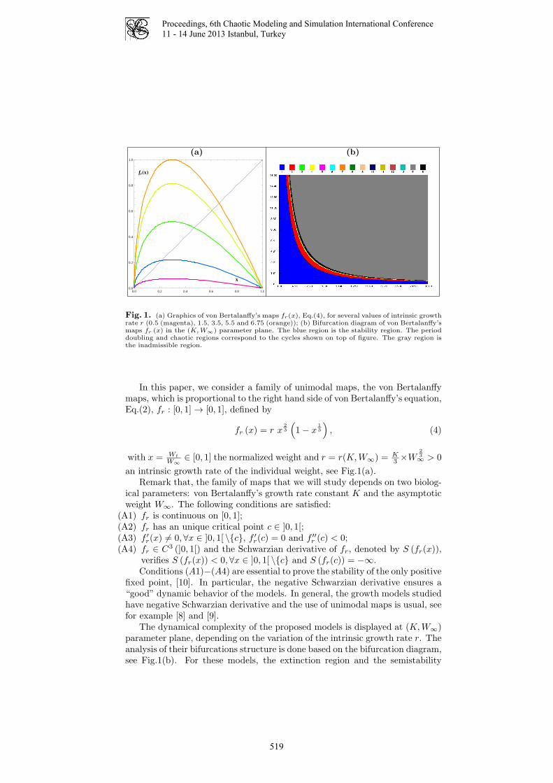
Proceedings, 6th Chaotic Modeling and Simulation International Conference
11 - 14 June 2013 Istanbul, Turkey
(a) (b)
x
frHxL
0.0 0.2 0.4 0.6 0.8 1.00.0
0.2
0.4
0.6
0.8
1.0
Fig. 1. (a) Graphics of von Bertalanffy’s maps fr(x), Eq.(4), for several values of intrinsic growthrate r (0.5 (magenta), 1.5, 3.5, 5.5 and 6.75 (orange)); (b) Bifurcation diagram of von Bertalanffy’smaps fr (x) in the (K,W∞) parameter plane. The blue region is the stability region. The perioddoubling and chaotic regions correspond to the cycles shown on top of figure. The gray region isthe inadmissible region.
In this paper, we consider a family of unimodal maps, the von Bertalanffymaps, which is proportional to the right hand side of von Bertalanffy’s equation,Eq.(2), fr : [0, 1] → [0, 1], defined by
fr (x) = r x23
(
1− x13
)
, (4)
with x = Wt
W∞
∈ [0, 1] the normalized weight and r = r(K,W∞) = K3 ×W
23∞ > 0
an intrinsic growth rate of the individual weight, see Fig.1(a).Remark that, the family of maps that we will study depends on two biolog-
ical parameters: von Bertalanffy’s growth rate constant K and the asymptoticweight W∞. The following conditions are satisfied:
(A1) fr is continuous on [0, 1];(A2) fr has an unique critical point c ∈ ]0, 1[;(A3) f ′
r(x) 6= 0, ∀x ∈ ]0, 1[ \c, f ′
r(c) = 0 and f ′′
r (c) < 0;(A4) fr ∈ C3 (]0, 1[) and the Schwarzian derivative of fr, denoted by S (fr(x)),
verifies S (fr(x)) < 0, ∀x ∈ ]0, 1[ \c and S (fr(c)) = −∞.Conditions (A1)−(A4) are essential to prove the stability of the only positive
fixed point, [10]. In particular, the negative Schwarzian derivative ensures a“good” dynamic behavior of the models. In general, the growth models studiedhave negative Schwarzian derivative and the use of unimodal maps is usual, seefor example [8] and [9].
The dynamical complexity of the proposed models is displayed at (K,W∞)parameter plane, depending on the variation of the intrinsic growth rate r. Theanalysis of their bifurcations structure is done based on the bifurcation diagram,see Fig.1(b). For these models, the extinction region and the semistability
519

Proceedings, 6th Chaotic Modeling and Simulation International Conference
11 - 14 June 2013 Istanbul, Turkey
curve have no expressive meaning. Because it is difficult to identify per capita
growth rates, Eq.(3), less than one for all densities, to the extinction case, andper capita growth rates strictly less than one for all densities, except at onepopulation density, to the semistability case, except at most a set of measurezero. We verify that, lim
x→0+f
′
r (x) > 1 and the origin’s basin of attraction is
empty, except at most a set of measure zero. The fixed point 0 is unstable.
A behavior of stability is defined when a population persists for intermedi-ate initial densities and otherwise goes extinct. The per capita growth rate ofthe population, Eq.(3), is greater than one for an interval of population densi-ties. The lower limit of these densities correspond to the positive fixed pointAK,W∞
≡ Ar, of each function fr, Eq.(4), see Fig.1(a). Furthermore, attendingto (A2) and (A3) we have that f2
r (c) > 0, then there is a linearly stable fixedpoint Ar ∈ ]0, 1[, whose basin of attraction is ]0, 1[, for more details see [10].
The symbolic dynamics techniques prove to be a good method to determinea numerical approximation to the stability region (in blue), see Fig.1(b). Formore details about symbolic dynamics techniques see for example [8]. In the(K,W∞) parameter plane, this region is caracterized by the critical point iter-ates that are always attracted to the fixed point sufficiently near of the superstable or super attractive point Ar, defined by fr (c) = c. Let Ar ∈ ]0, 1[ bethe fixed points sufficiently near of Ar, then
limn→∞
fnr (c) = Ar, for
(
3K−1A13r
(
1−A13r
))32
< W∞(K) < W∞(K)
where W∞(K) represents the super stabel curve of the cycle of order 2, given inimplicit form by f2
r (c) = c. In this parameter plane, the set of the super stableor super attractive points Ar defines the super stabe curve of the fixed point.In the region before reaching the super stable curve, the symbolic sequencesassociated to the critical points orbits are of the type CL∞. After this superstable curve, the symbolic sequences are of the type CR∞. In this parameterregion, the topological entropy is null, [6].
The period doubling region corresponds to the parameters values, to whichthe population weight oscillates asymptotically between 2n states, with n ∈ N.In period-dubling cascade, the symbolic sequences correspondent to the iteratesof the critical points are determined by the iterations f2n
r (c) = c. Analytically,these equations define the super-stability curves of the cycle of order 2n. Theperiod doubling region is bounded below by the curve of the intrinsic growthrate values where the period doubling starts, W∞(K), correspondent to the2-period symbolic sequences (CR)∞. Usually, the upper limit of this region isdetermined using values of intrinsic growth rate r, corresponding to the firstsymbolic sequence with non null topological entropy. Commonly, the symbolicsequence that identifies the beginning of chaos is
(
CRLR3)
∞
, a 6-periodicorbit, see for example [8] and [9]. The unimodal maps in this region, also havenull topological entropy, [6].
In the chaotic region of the (K,W∞) parameter plane, the evolution ofthe population size is a priori unpredictable. The maps are continuous onthe interval with positive topological entropy whence they are chaotic and
520

Proceedings, 6th Chaotic Modeling and Simulation International Conference
11 - 14 June 2013 Istanbul, Turkey
the Sharkovsky ordering is verified. The symbolic dynamics are characterizedby iterates of the functions fr that originate orbits of several types, whichalready present chaotic patterns of behavior. The topological entropy is a non-decreasing function in order to the parameter r, until reaches the maximumvalue ln 2 (consequence of the negative Schwartzian derivative). In [8] and[9] can be seen a topological order with several symbolic sequences and theirtopological entropies, which confirm this result to others growth models. Thisregion is bounded below by the curve of the intrinsic growth rate values wherethe chaos starts. The upper limit is the fullshift curve, defined by fr (c) = 1.This curve characterizes the transition between the chaotic region and theinadmissible region. In the inadmissible region, the graphic of any function fris no longer totally in the invariant set [0, 1]. The maps under these conditionsnot already belong to the studied familie functions and are not good modelsfor populations dynamics.
3 Synchronization and Lyapunov exponents
Consider a general network ofN identical coupled dynamical systems, describedby a connected, undirected graph, with no loops and no multiple edges. In eachnode the dynamics of the system is defined by the maps fr given by Eq.(4).The state equations of this network, in the discretized form, are
xi(k + 1) = fr(xi(k)) + c
N∑
j=1
lijfr(xj(k)), with i = 1, 2, ..., N (5)
where c is the coupling parameter and L = (lij) is the Laplacian matrix orcoupling configuration of the network. The Laplacian matrix is given by L =D − A, where A is the adjacency matrix and D = (dij) is a diagonal matrix,with dii = ki, being ki the degree of node i. The eigenvalues of L are all realand non negatives and are contained in the interval [0,min N, 2∆], where∆ isthe maximum degree of the vertices. The spectrum of L may be ordered, λ1 =0 ≤ λ2 ≤ · · · ≤ λN . The network (5) achieves asymptotical synchronization if
x1(t) = x2(t) = ... = xN (t) →t→∞
e(t),
where e(t) is a solution of an isolated node (equilibrium point, periodic orbitor chaotic attractor), satisfying e(t) = f(e(t)).
One of the most important properties of a chaotic system is the sensitivityto initial conditions. A way to measure the sensitivity with respect to initialconditions is to compute the average rate at which nearby trajectories divergefrom each other. Consider the trajectories xk and yk, starting, respectively,from x0 and y0. If both trajectories are, until time k, always in the same linearregion, we can write
|xk − xk| = eλk|x0 − y0|, where λ =1
k
k−1∑
j=0
ln |f ′
r(xj)|.
521

Proceedings, 6th Chaotic Modeling and Simulation International Conference
11 - 14 June 2013 Istanbul, Turkey
r
hmax
2 3 4 5 6-5
-4
-3
-2
-1
0
1
2
Fig. 2. Lypunov exponents estimates for von Bertalanffy’s maps Eq.(4), as a function of theintrinsic growth rate r.
The Lyapunov exponents of a trajectory xk is defined by
hmax = limk→+∞
1
k
k−1∑
j=0
ln |f ′
r(xj)| (6)
whenever it exists. The computation of the Lyapunov exponent hmax gives theaverage rate of divergence (if hmax > 0), or convergence (if hmax < 0) of the twotrajectories from each other, during the time interval [0, k], see for example [16].We note that, the Lyapunov exponents depend on two biological parameters:von Bertalanffy’s growth rate constant and the asymptotic weight. See in Fig.2the Lyapunov exponents estimate for von Bertalanffy’s maps Eq.(4).
If the coupling parameter c belongs to the synchronization interval]
1− e−hmax
λ2,1 + e−hmax
λN
[
(7)
then the synchronized states xi(t), (i = 1, ...N) are exponentially stable, [17].The second eigenvalue λ2 is know as the algebraic connectivity or Fiedler valueand plays a special role in the graph theory. As bigger is λ2, more easilythe network synchronizes. As much larger λ2 is, more difficult is to separatethe graph in disconnected parts. The graph is connected if and only if λ2 6=0. In fact, the multiplicity of the null eigenvalue λ1 is equal to the numberof connected components of the graph. Fixing the topology of the network,the eigenvalues of the Laplacian λ2 and λN are fixed, so the synchronizationonly depends on the Lyapunov exponent of each node, hmax. Remark thatthe synchronization interval also depend on two biological parameters: vonBertalanffy’s growth rate constant and the asymptotic weight.
4 Numerical simulation and conclusions
To support our approaches, we consider a regular ring lattice, a graph with N
nodes, each one connected to k neighbors, k2 on each side, having in each node
the same model, the von Bertalanffy maps fr given by Eq.(4). See in Fig.3
522

Proceedings, 6th Chaotic Modeling and Simulation International Conference
11 - 14 June 2013 Istanbul, Turkey
1
2
34
5
6
1 2
34
a b c)))1
2
34
5
6
Fig. 3. Lattices. In a) with N = 4 nodes and k = 2, in b) with N = 6 nodes and k = 2 and in c)with N = 6 nodes and k = 4. From (a) to (b) the total number of vertices of the network increasesmaintaining the number of neighbors of each node, and from (b) to (c) increases the number ofneighbors of each node, but the total number of vertices of the network remains the same.
some example of lattices. If, for instance, N = 6 and K = 4, see Fig.3c), theadjacency matrix A and the Laplacian matrix L are
A =
0 1 1 0 1 11 0 1 1 0 11 1 0 1 1 00 1 1 0 1 11 0 1 1 0 11 1 0 1 1 0
and L = D −A =
4 −1 −1 0 −1 −1−1 4 −1 −1 0 −1−1 −1 4 −1 −1 00 −1 −1 4 −1 −1−1 0 −1 −1 4 −1−1 −1 0 −1 −1 4
.
So, the network correspondent to the graph in Fig.3 c) is defined by the system,
x1 = fr(x1) + c(4x1 − x2 − x3 − x5 − x6)x2 = fr(x2) + c(−x1 + 4x2 − x3 − x4 − x6)x3 = fr(x3) + c(−x1 − x2 + 4x3 − x4 − x5)x4 = fr(x4) + c(−x2 − x3 + 4x4 − x5 − x6)x5 = fr(x5) + c(−x1 − x3 − x4 + 4x5 − x6)x6 = fr(x6) + c(−x1 − x2 − x4 − x5 + 4x6)
.
For this lattice the eigenvalues of the Laplacian matrix are λ1 = 0, λ2 =λ3 = λ4 = 4 and λ5 = λ6 = 6. If we consider, for instance, r = 6.60, theLyapunov exponent of fr(x) is 0.377, Eq.(6). Then, attending to Eq.(7), this
lattice synchronizes if 1−e−0.377
2 < c < 1+e−0.377
6 ⇔ 0.079 < c < 0.281 and theamplitude of the synchronization interval is 0.202. For more examples see Table1. The lattice correspondent to the Fig.3 b) has eigenvalues of the Laplacianmatrix λ1 = 0, λ2 = λ3 = 1, λ4 = λ5 = 3 and λ6 = 4. Thus, for the samer = 6.60, the lattice synchronizes if 0.313 < c < 0.421 and the amplitude ofthis interval is 0.107. Moreover, to the lattice in Fig.3 a), the eigenvalues of theLaplacian matrix are λ1 = 0, λ2 = λ3 = 2 and λ4 = 4. For the same r = 6.60,the lattice synchronizes if 0.157 < c < 0.421 and the amplitude of this intervalis 0.264. In Table 1 are presented more examples, where we computed thesynchronization interval for several values of the intrinsic growth rate r, for allthese lattices a), b) and c) of Fig.3. The results of Table 1 allow us to claim:
(C1) From the lattice a) to lattice b) in Fig.3, the total number of vertices ofthe network increases maintaining the number of neighbors of each node.
523

Proceedings, 6th Chaotic Modeling and Simulation International Conference
11 - 14 June 2013 Istanbul, Turkey
Synchronization Interval Amplituder hmax
Lattice a) Lattice b) Lattice c) Lattice a) Lattice b) Lattice c)
6.50 0.297 ]0.128, 0.436[ ]0.257, 0.436[ ]0.064, 0.291[ 0.308 0.179 0.226
6.55 0.347 ]0.147, 0.427[ ]0.293, 0.427[ ]0.073, 0.285[ 0.280 0.134 0.211
6.60 0.377 ]0.157, 0.421[ ]0.313, 0.421[ ]0.079, 0.281[ 0.264 0.107 0.202
6.65 0.406 ]0.167, 0.417[ ]0.334, 0.417[ ]0.083, 0.278[ 0.250 0.083 0.194
6.70 0.463 ]0.185, 0.407[ ]0.371, 0.407[ ]0.093, 0.272[ 0.222 0.037 0.179
6.73 0.506 ]0.199, 0.401[ ]0.397, 0.401[ ]0.099, 0.267[ 0.202 0.003 0.168
6.74 0.533 ]0.207, 0.397[ (*) ]0.103, 0.265[ 0.190 (*) 0.161
6.75 0.598 ]0.225, 0.388[ (*) ]0.112, 0.258[ 0.163 (*) 0.146
Table 1. Lyapunov exponent, hmax, synchronization interval,]
1−e−hmax
λ2, 1+e
−hmax
λN
[
, and
amplitude of this interval, 1+e−hmax
λN−
1−e−hmax
λ2, for several intrinsic growth rates r, for the
lattices a), b) and c) of Fig.3.(*) In this case, the desynchronization phenomenon occurs, see (C4).
We verify that the synchronization is worse, not only because it begins tosynchronize at a higher value of the coupling parameter c, but also, becausethe synchronization interval is shorter.
(C2) Comparing the results for the lattices b) and c) in Fig.3, we may concludethat maintaining the total number of vertices of the network, but increas-ing the number of neighbors of each node, the synchronization is better,not only because it begins to synchronize at a lower value of the couplingparameter c, but also, because the synchronization interval is larger.
(C3) Observing the columns of Table 1, we verify that, as the intrinsic growthrate r increases, the synchronization is worse, not just because it begins tosynchronize at a higher value of the coupling parameter c, but also, becausethe synchronization interval is shorter.
(C4) Note that, for the intrinsic growth rate r = 6.74 and r = 6.75, for the latticeb), the upper bound of the synchronization interval is lower than the lowerbound. This means that, there is no synchronization for any value of thecoupling parameter c. This desynchronization phenomenon was expectedbecause the network (5) synchronizes only if hmax < ln(2R + 1), whereR = λ1−λ2
λ2−λN
, see [17]. In the case of lattice b), we have ln(2R+1) = 0.511, sothere is synchronization only if hmax < 0.511, which do not happens for r =6.74 and r = 6.75. In all the other studied cases, the Lyapunov exponentverifies hmax < ln(2R+1), so we have a non empty synchronization interval.
524
Proceedings, 6th Chaotic Modeling and Simulation International Conference
11 - 14 June 2013 Istanbul, Turkey
Acknowledgment
Research partially sponsored by national funds through the Foundation for Sci-ence and Technology, Portugal - FCT under the project PEst-OE/MAT/UI0006/2011, CEAUL, CIMA-UE and ISEL. The authors are grateful to Prof. DanieleFournier-Prunaret for having made the image of Fig.1(b).
References
1.G.M. Cailliet, W.D. Smith, H.F. Mollet and K.J. Goldman. Age and growth studiesof chondrichthyan fishes: the need for consistency in terminology, verification,validation, and growth function fitting. Environ. Biol. Fish., 77: 211–228, 2006.
2.A.B. Cooper. A Guide to Fisheries Stock Assessment. From Data to Recommenda-tions. New Hampshire Sea Grant, 2006.
3.T.E. Essington, J.F. Kitchell and C.J. Walters. The von Bertalanffy growth func-tion, bioenergetics, and the consumption rates of fish. Can. J. Fish. Aquat. Sci.,58: 2129–2138, 2001.
4.J.A. Hutchings and J.D. Reynolds. Marine fish population collapses: consequencesfor recovery and extinction isk. BioSci., 54: 297–309, 2004.
5.V.S. Karpouzi and D. Pauly. Life-History Patterns in Marine Birds. In M.L.D.Palomares and D. Pauly, editors, Fisheries Centre Research Reports 16 (10),Von Bertalanffy Growth Parameters of Non-Fish Marine Organisms, pages 27-43, Canada, 2008. The Fisheries Centre, University of British Columbia.
6.D. Lind and B. Marcus. An Introduction to Symbolic Dynamics and Codings. 2nd
edition, Cambridge University Press, Cambridge, 1999.7.J.A. Musick. Criteria to define extinction risk in marine fishes. Fisheries, 24: 6–14,
1999.8.J.L. Rocha and S.M. Aleixo. An extension of gompertzian growth dynamics: Weibull
and Frechet models. Math. Biosci. Eng., 10: 379–398, 2013.9.J.L. Rocha and S.M. Aleixo. Dynamical analysis in growth models: Blumberg’s
equation. Discrete Contin. Dyn. Syst.-Ser.B, 18: 783–795, 2013.10.S.J. Schreiber. Chaos and population disappearances in simple ecological models.
J. Math. Biol., 42: 239–260, 2001.11.L. Von Bertalanffy. A quantitative theory of organic growth. Human Biology, 10:
181–213, 1938.12.L. Von Bertalanffy. Quantitative laws in metabolism and Growth. The Quarterly
Review of Biology, 32: 217–231, 1957.13.A. Balanov, N. Janson, D. Postnov and O. Sosnovtseva. Synchronization: From
Simple to Complex, Springer, 2009.14.A.J. Davidson and M. Menaker, Birds of a feather clock together sometimes: social
synchronization of circadian rhythms. Curr. Opin. Neurobiol., 13 (6): 765–769,2003.
15.J.A.L. Silva and F.T. Giordani, Density-dependent migration and synchronism inmetapopulations. Bull. of Math. Bio-, 68: 451-465, 2006.
16.M.Hasler and Y.L. Maistrenko, An introduction to the synchronization of chaoticsystems: coupled skew tent maps. IEEE Trans. on Circ. Syst. – I, 44 (10): 856–866, 1987.
17.X. Li and G. Chen, Synchronization and desynchronization of complex dynamicalnetworks: An engineering viewpoint. IEEE Trans. on Circ. Syst. –I, 50 (11):1381–1390, 2003.
525

Proceedings, 6th Chaotic Modeling and Simulation International Conference
11 - 14 June 2013 Istanbul, Turkey
526

Proceedings, 6th Chaotic Modeling and Simulation International Conference
11 - 14 June 2013 Istanbul, Turkey
Mutual information rate and topological orderin networks
J. Leonel Rocha1 and Acilina Caneco2
1 Instituto Superior de Engenharia de Lisboa - ISEL, ADM and CEAUL, RuaConselheiro Emıdio Navarro, 1, 1959-007 Lisboa, Portugal(E-mail: [email protected]),
2 Instituto Superior de Engenharia de Lisboa - ISEL, ADM and CIMA-UE, RuaConselheiro Emıdio Navarro, 1, 1959-007 Lisboa, Portugal(E-mail: [email protected])
Abstract. In this paper we study the evolution of the information flow associatedwith a topological order in networks. The amount of information produced by anetwork may be measure by the mutual information rate. This measure and the syn-chronization interval are expressed in terms of the transversal Lyapunov exponents.The networks are constructed by successively joining one edge, maintaining the samenumber of nodes, and the topological order is described by the monotonicity of thenetwork topological entropy. The network topological entropy measures the complex-ity of the network topology and it is expressed by the Perron value of the adjacencymatrix. We conclude that, as larger the network topological entropy, the larger isthe rate with which information is exchanged between nodes of such networks. Toillustrate our ideas we present numerical simulations for several networks with a topo-logical order established.Keywords: Mutual information rate, topological entropy, networks.
1 Introduction and motivation
Information theory is an area of mathematics and engineering, concerning thequantification of information and it benefits of matters like mathematics, statis-tics, computer science, physics, neurobiology and electrical engineering. Infor-mation theory and synchronization are directly related in a network. Theentropy is a fundamental measure of information content and the topologicalentropy can describe the character of complexity of a network, see for example[10]. In [6], using the mutual information rate to measure the information flow,we have proved that the larger the synchronization is, the larger is the ratewith which information is exchanged between nodes in the network. Althoughthe important growth in the field of complex networks, it is still not clearwhich conditions for synchronization implies information transmission and itis still not known which topology is suitable for the flowing of information.Nevertheless, we conclude with this study that, the more complex is a network,expressed by its topological entropy, the larger is the flux of information.
In this work we study the relationship between the topological order in net-works and the transmission of information. The topological order in networks isdescribed by the monotonicity of the network topological entropy. The conceptof the network topological entropy was previously introduced in [10]. However,
527
Proceedings, 6th Chaotic Modeling and Simulation International Conference
11 - 14 June 2013 Istanbul, Turkey
there are several concepts of network entropy, see [7]. We will use the onebased on symbolic dynamics. In Sec.2, we present some preliminaries conceptsto be used in the following, such as: fundamental notions of graphs theory,conditions for complete synchronization, comunication channel and mutual in-formation rate. Sec.3 is devoted to the study of topological order in networks,using the definition of the network topological entropy. In Sec.4, numerical sim-ulations are presented for several networks with a topological order established.Finally, in Sec.5, we discuss our study and provide some relevant conclusions.
2 Preliminaries concepts
In this section, we introduce some notions and basic results on graphs andnetworks theory. Mathematically, networks are described by graphs (directedor undirected) and the theory of dynamical networks is a combination of graphtheory and nonlinear dynamics. From the point of view of dynamical systems,we have a global dynamical system emerging from the interactions between thelocal dynamics of the individual elements. The tool of graph theory allows usto analyze the coupling structure between them.
A graph G is an ordered pair G = (V,E), where V is a nonempty set ofN vertices or nodes vi and E is a set of edges or links, eij , that connect twovertices vi and vj . We will only consider the case of undirected graphs, thatmeans that the edge eij is the same as the edge eji. If the graph G is notweighted, the adjacency matrix A = A (G) = [aij ] is defined as follows:
aij =
1, if vi and vj are connected0, if vi and vj are not connected
.
The degree of a node vi is the number of edges incident on it and is denotedby ki. For more details in graph theory see [4].
Consider a network of N identical chaotic dynamical oscillators, describedby a connected and undirected graph, with no loops and no multiple edges.In each node the dynamics of the oscillators is defined by xi = f(xi), withf : Rn → Rn and xi ∈ Rn is the state variables of the node i. The stateequations of this network are
xi = f(xi) + σN∑j=1
lij xj , with i = 1, 2, ..., N (1)
where σ > 0 is the coupling parameter, L = [lij ] = A − D is the Laplacianmatrix or coupling configuration of the network. One of the most importantsubjects under investigation is the network synchronizability, fixing the con-nection topology and varying the local dynamics or fixing the local dynamicand varying the connection topology [5]. In [9] it was establish that completesynchronization can be achieved provided that all the conditional Lyapunovexponents are negative. In Sec.4, we use this result to determine the synchro-nization interval. The negativity of the conditional Lyapunov exponents is anecessary condition for the stability of the synchronized state, [3]. It is also amathematical expression of the decreasing to zero of the logarithm average of
528

Proceedings, 6th Chaotic Modeling and Simulation International Conference
11 - 14 June 2013 Istanbul, Turkey
the distance of the solutions on the transverse manifold to the solutions on thesynchronization manifold.
A communication channel represents a pathway through which informationis exchanged. In this work, a communication channel is considered to be formedby a transmitter Si and a receiver Sj , where the information about the trans-mitter can be measured. In a network, each one of the links between them, i.e.,each one of the edges of the corresponding graph, represents a communicationchannel. In [1], it is defined the mutual information rate (MIR) between onetransmitter Si and one receiver Sj , denoted by IC(Si, Sj), by
IC(Si, Sj) =
λ∥ − λ⊥ , if λ⊥ > 0
λ∥ , if λ⊥ ≤ 0, (2)
where λ∥ denotes the positive Lyapunov exponents associated to the synchro-nization manifold and λ⊥ denotes the positive Lyapunov exponents associatedto the transversal manifold, between Si and Sj . λ∥ represents the information(entropy production per time unit) produced by the synchronous trajectoriesand corresponds to the amount of information transmitted. On the other hand,λ⊥ represents the information produced by the nonsynchronous trajectories andcorresponds to the information lost in the transmission, the information thatis erroneously retrieved in the receiver. For more details and references see forexample [1] and [2]. In [6], we prove that as the coupling parameter increases,the mutual information rate increases to a maximum at the synchronizationinterval and then decreases.
3 Topological order in networks
In this section we study a topological order in networks, which are constructedby successively joining one edge, maintaining the same number of nodes. Thistopological order is described by the monotonicity of the network topologicalentropy. The introduction of the network topological entropy concept was madein [10], which requires a strict and long construction, using tools of symbolicdynamics and algebraic graph theory. However, we present some basic aspectsof this definition. The topological entropy htop(X) of a shift dynamical system(X,σ) over some finite alphabet A is defined by
htop(X) = limn→∞
log Tr (An(X))
n
and htop(X) = 0 if X = ∅, where A(X) is the transition matrix of X, [8].We remark that the transition matrix A(X) describes the dynamics betweenthe nodes of the network, which is represented by a graph G. The Perron-Frobenius Theorem states that, if the adjacency matrix A = 0 is irreducibleand λA is the Perron value of A, then htop(X) = log λA. We calculate thetopological entropy of the associated dynamical system, which is equal to thelogarithm of the growth rate of the number of admissible words, [8]. If we havea network associated to a graph G, which determine the shift space X, we willcall network topological entropy of G the quantity htop(X), i.e.,
htop(G) = htop(X) = log λA. (3)
529

Proceedings, 6th Chaotic Modeling and Simulation International Conference
11 - 14 June 2013 Istanbul, Turkey
The following result establishes a topological order in networks.
Proposition 1. Let G1 and G2 be two undirected graphs, with the same num-ber of vertices N , and G1 be a not complete graph. If the graph G2 is obtainedfrom the graph G1 by joining an edge, then htop(G2) > htop(G1).
Proof. Let A = [aij ] and B = [bij ] be the adjacency matrices of the graphs G1
and G2, respectively. If the graph G2 is obtained from the graph G1 by joiningan edge, then the adjacency matrix B is obtained from the adjacency matrixA by replacing some entry aij = 0 by bij = 1. As the graphs G1 and G2 arenot directed, then the matrices A and B are symmetric, and bji = 1. Thus,the matrix B is equal to the matrix A plus some matrix with non negativeentries. For any power n, we have Bn = An + C, for some matrix C whoseentries are all non negative. As Tr(C) ≥ 0 and Tr(Bn) = Tr(An) + Tr(C),
then Tr(Bn) > Tr(An). Consequently, we obtain log Tr(Bn)n > log Tr(An)
n , forall integers n. From the definition of network topological entropy, Eq.(3), wehave htop(G2) > htop(G1).
4 Numerical simulations
In this section we will consider, as an example, a network with N = 6 nodes,having in each node the same skew-tent map, f : [0, 1] → [0, 1], defined by
f(x) =
xa , if 0 ≤ x ≤ a
1−x1−a , if a < x ≤ 1
, (4)
with 0.5 ≤ a < 1, see [6]. See Fig.1 where we present some examples of thesenetworks. We start with a network of 7 edges, without the edges 1− 2, 3− 5,5− 6, 3− 4, 4− 6, 2− 5, 3− 6 and 2− 4, and each time we add one edge, thelast one of this list. We evaluate the eigenvalues of the Jacobian matrix, theLyapunov exponents, the region where all transversal Lyapunov exponents arenegatives, the synchronization interval and the mutual information rate for allcommunication channels of these networks. In order to compare the results, aswe add one edge, we consider for all studied cases the same value a = 0.9 of theskew-tent map parameter. For this network, the region where all transversalLyapunov exponents are negatives do not intersect the line a = 0.9. So, forthis value of a there is no synchronization interval, see 1) of Fig.2, and we donot evaluate the mutual information rate in this case.
We present the details for the network with 8 edges shown in 1) of Fig.1.The adjacency matrix A and the Laplacian matrix L of this network are:
A =
0 0 1 1 1 10 0 1 1 0 11 1 0 0 0 01 1 0 0 1 01 0 0 1 0 01 1 0 0 0 0
and L = A−D =
−4 0 1 1 1 10 −3 1 1 0 11 1 −2 0 0 01 1 0 −3 1 01 0 0 1 −2 01 1 0 0 0 −2
,
530

Proceedings, 6th Chaotic Modeling and Simulation International Conference
11 - 14 June 2013 Istanbul, Turkey
1
23
4
5 6
1
23
4
5 6
1
23
4
5 6
1
23
4
5 6
1) 2) 3) 4)
Fig. 1. Construction of networks by successively joining one edge, with 8, 10, 14 and 15 edgesand N = 6 nodes.
σ
a
1) 2) 3)
Fig. 2. Regions where the transversal Lyapunov exponents are negatives. The synchronizationregion is the intersection of these regions. In the vertical axis is the coupling parameter σ and in thehorizontal axis is the tent map parameter a. In 1) is the network with 7 edges, in 2) with 8 edges,and in 3) with 9 edges. The image in 1) shows that for a = 0.9 there is no synchronization intervalbecause the intersection of the regions where all transversal Lyapunov exponents are negativesdoes not occur for a = 0.9.
where D is the diagonal matrix with entries dii = ki, beeing ki the degree ofeach node i. This network is defined by the following system,
x1 = f(x1) + σ(−4x1 + x3 + x4 + x5 + x6)x2 = f(x2) + σ(−3x2 + x3 + x4 + x6)x3 = f(x3) + σ(x1 + x2 − 2x3)x4 = f(x4) + σ(x1 + x2 − 3x4 + x5)x5 = f(x5) + σ(x1 + x4 − 2x5)x6 = f(x6) + σ(x1 + x2 − 2x6)
,
where σ is the coupling parameter. The Jacobian matrix is given by,
J =
c− 4σ 0 σ σ σ σ
0 c− 3σ σ σ 0 σσ σ c− 2σ 0 0 0σ σ 0 c− 3σ σ 0σ 0 0 σ c− 2σ 0σ σ 0 0 0 c− 2σ
,
being c = c(x) the slope of f , Eq.(4), given by c(x) = 1a , if x ≤ a and
c(x) = − 11−a if x > a. The eigenvalues of the Jacobian are µ1 = c, µ2 = c−4σ,
µ3 = c − 3σ, µ4 = c − 2σ, µ5 = c − 72σ −
√172 and µ6 = c − 7
2σ −√172 . The
531

Proceedings, 6th Chaotic Modeling and Simulation International Conference
11 - 14 June 2013 Istanbul, Turkey
0.0 0.2 0.4 0.6 0.8 1.0 1.2 1.4
0.0
0.1
0.2
0.3
0.4
0.5
0.0 0.2 0.4 0.6 0.8 1.0 1.20.0
0.1
0.2
0.3
0.4
0.5
1) 2)
IC2IC3
IC4
IC6IC5 IC1
IC2
IC3
σσ
Fig. 3. ICifor the network with 8 edges in 1) of Fig.1 and with 10 edges in 2) of Fig.1.
first eigenvector is (1, 1, 1, 1, 1, 1) and it corresponds to the parallel Lyapunovexponent λ∥. The others eigenvectors correspond to the transversal Lyapunovexponents λ⊥i , with i = 2, 3, 4, 5, 6. So, the parallel Lyapunov exponent is
λ∥ =
∫ln |µ1| =
∫ a
0
ln1
a+
∫ 1
a
ln
∣∣∣∣ −1
1− a
∣∣∣∣ = −a ln a− (1− a) ln(1− a) (5)
and the transversal Lyapunov exponents are
λ⊥i = a ln
∣∣∣∣1a − νiσ
∣∣∣∣+ (1− a) ln
∣∣∣∣− 1
1− a− νiσ
∣∣∣∣ , with i = 2, 3, 4, 5, 6
where ν2 = 4, ν3 = 3, ν4 = 2, ν5 = 72σ +
√172 and ν6 = 7
2σ −√172 . In order to
have synchronization, all transversal Lyapunov exponents must be negatives,see 2) in Fig.2. In this figure, each color corresponds to a region where one ofthe transversal Lyapunov exponents is negative. For example, if a = 0.9, thenthe synchronization interval is ]0.236, 0.336[, where all the transversal Lyapunovexponents λ⊥i are negative. See also 3) in Fig.2 for the network with 9 edges.To evaluate the mutual information rate (MIR), according to Eq.(2), for eachλ⊥i we obtain the interval ]ai, bi[ where λ⊥i < 0, thus
ICi =
−a ln a− (1− a) ln(1− a)− a ln
∣∣ 1a − νiσ
∣∣− (1− a) ln∣∣∣− 1
1−a − νiσ∣∣∣ ,
if σ < ai or σ > bi−a ln a− (1− a) ln(1− a), if ai < σ < bi
with a = 0.9 and i = 2, 3, 4, 5, 6. See in 1) of Fig.3 the plots of these ICi .The MIR attains its maximum 0.325..., in an interval of lenght 1.028 and thenetwork topological entropy, given by Eq.(3), is log λA = 1.02835....
The second case that we study in detail is the network with 10 edges andwithout the edges, see 2) of Fig.1. The adjacency matrix A and the Laplacianmatrix L are given by,
A =
0 0 1 1 1 10 0 1 1 1 11 1 0 0 0 11 1 0 0 1 01 1 0 1 0 01 1 1 0 0 0
and L = A−D =
−4 0 1 1 1 10 −4 1 1 1 11 1 −3 0 0 11 1 0 −3 1 01 1 0 1 −3 01 1 1 0 0 −3
.
532

Proceedings, 6th Chaotic Modeling and Simulation International Conference
11 - 14 June 2013 Istanbul, Turkey
This network is defined by the system,
x1 = f(x1) + σ(−4x1 + x3 + x4 + x5 + x6)x2 = f(x2) + σ(−4x2 + x3 + x4 ++x5 + x6)x3 = f(x3) + σ(x1 + x2 − 3x3 + x4)x4 = f(x4) + σ(x1 + x2 − 3x4 + x5)x5 = f(x5) + σ(x1 + x2 + x4 − 3x5)x6 = f(x6) + σ(x1 + x2 + x3 − 3x6)
,
and the Jacobian matrix is given by
J =
c− 4σ 0 σ σ σ σ
0 c− 4σ σ σ σ σσ σ c− 3σ σ 0 0σ σ σ c− 3σ σ 0σ σ 0 σ c− 3σ 0σ σ σ 0 0 c− 3σ
.
The eigenvalues of the Jacobian matrix are µ1 = c, µ2 = c − 6σ, µ3 = µ4 =µ5 = c−4σ and µ5 = c−2σ. Thus, the parallel Lyapunov exponent is identicalto the previous case, Eq.(5), and the transversal Lyapunov exponents are
λ⊥i = a ln
∣∣∣∣1a − νiσ
∣∣∣∣+ (1− a) ln
∣∣∣∣− 1
1− a− νiσ
∣∣∣∣ , with i = 2, 3, 4
where ν2 = 6, ν3 = 4 and ν4 = 2. See 1) in Fig.4 the regions where thesetransversal Lyapunov exponents are negatives. For a = 0.9, this networksynchronizes if σ ∈]0.170, 0.312[. We compute the ICi like in the previouscase and we plot its graphics in 2) of Fig.3. The MIR attains its maximum0.325..., in an interval of lenght 1.216 and the network topological entropy islog λA = 1.21559.... Figs.4, 5 and Table 1 contain information similar to theother cases analyzed in this topological order.
2) 3)
σ
1) 2) 3)
a
Fig. 4. Regions where the transversal Lyapunov exponents are negatives. The synchronizationregion is the intersection of these regions. In 1) is the network with 10 edges, in 2) with 11 edges,and in 3) with 12 edges. For the same value of a, the amplitude of the synchronization intervalincreases.
533

Proceedings, 6th Chaotic Modeling and Simulation International Conference
11 - 14 June 2013 Istanbul, Turkey
2)
σ
a
1) 3)
Fig. 5. Regions where the transversal Lyapunov exponents are negatives. The synchronizationregion is the intersection of these regions. In 1) is the network with 13 edges, in 2) with 14edges and in 3) with 15 edges (complete network). For the same value of a, the amplitude of thesynchronization interval increases.
Edges µi = c− νiσ (i = 2, 3, 4, 5, 6) Sync. interv. Ampl. log λA
8 ν2 = 4, ν3 = 3, ν4 = 2, ν5 = 7+√
172
, ν6 = 7−√
172
]0.236,0.336[ 0.100 1.028
9 ν2 = ν3 = 4, ν4 = 3, ν5 = 7+√
172
, ν6 = 7−√
172
]0.236,0.336[ 0.100 1.127
10 ν2 = 6, ν3 = ν4 = ν5 = 4, ν6 = 2 ]0.170,0.312[ 0.142 1.216
11 ν2 = 6, ν3 = ν4 = 4, ν5 = 4 +√2, ν6 = 4−
√2 ]0.131,0.312[ 0.181 1.312
12 ν2 = ν3 = 6, ν4 = 5, ν5 = 4, ν6 = 3 ]0.113,0.312[ 0.199 1.403
13 ν2 = ν3 = ν4 = 6 ν5 = ν6 = 4 ]0.085,0.312[ 0.227 1.475
14 ν2 = ν3 = ν4 = ν5 = 6 ν6 = 4 ]0.085,0.312[ 0.227 1.548
15 ν2 = ν3 = ν4 = ν5 = ν6 = 6 ]0.057,0.312[ 0.255 1.609
Table 1. Jacobian eigenvalues, µi, for (i = 2, 3, 4, 5, 6), which correspond to the transversalLyapunov exponents, synchronization interval, its amplitude, network topological entropy and thenumber of edges from 8 to 15 (complete network).
2 4 6 8 10 12 14edge number
0.5
1.0
1.5
top.entropy
Fig. 6. The network topological entropy increases as the the number of edges of the networkincreases.
5 Conclusions and discussion
We started our simulations, considering the network with 8 edges and withoutthe edges 1 − 2, 3 − 5, 5 − 6, 3 − 4, 4 − 6, 2 − 5 and 3 − 6, and in eachstep we add the last edge of this list. In each step of this construction, weobtain the Laplacian matrix and compute the eigenvalues µi (i = 1, 2, 3, 4, 5, 6)of the Jacobian matrix, the parallel and transversal Lyapunov exponents, the
534

Proceedings, 6th Chaotic Modeling and Simulation International Conference
11 - 14 June 2013 Istanbul, Turkey
synchronization interval, the network topological entropy and the ICifor the
networks with 8, 9, 10, 11, 12, 13, 14 and 15 edges (complete network). Forall these cases µ1 = c and this eigenvalue correspond to the synchronizationmanifold. The others µi correspond to the transversal Lyapunov exponents andare presented in Table 1. In this table is also presented the synchronizationinterval and the network topological entropy, for all these cases. See in Figs.2,4 and 5 the synchronization regions, in terms of the skew-tent map parametera and of the coupling parameter σ. In Fig.6 we may see that the networktopological entropy increases as we add one edge sucessively to the network.
From the numerical simulations shown in figures and Table 1, we concludethat, with the topological order established, the interval where the mutualinformation rate attains its maximum, the synchronization interval, increasesits amplitude. Thus, we claim that, as larger the network topological entropy,the larger is the rate with which information is exchanged between nodes inthe network.
Acknowledgment
This work is funded by FCT through the National Funds - Foundation for Sci-ence and Technology within the project PEst-OE/MAT/UI0006/2011, CIMA-UE, CEAUL and ISEL.
References
1.M. S. Baptista and J. Kurths, Chaotic channel, Phys. Rev. E, 72, 045202R, (2005).2.M. S. Baptista and J. Kurths, Information transmission in active networks, Phys.
Rev. E, 77, 026205, (2008).3.S. Boccaletti, J. Kurths, G. Osipov, D.L. Valladares and C.S. Zhou, The synchro-
nization of chaotic systems, Physics Reports, 366, 1-101, (2002).4.B. Bollobas and O.M. Riordan, Handbook of Graphs and Networks: From the
Genome to the Internet, Wiley-VCH, 2003.5.A. Caneco, S. Fernandes, C. Gracio and J.L. Rocha, Networks synchronizability,
local dynamics and some graph invariants, Dynamics, Games and Science I,Springer Proceedings in Mathematics, 1, 221-238, (2011).
6.A. Caneco and J.L. Rocha, Synchronization and information transmission in net-works, submited.
7.L. Ji, B.-H. Wang , W.-X. Wang and T. Zhou , Network entropy based on topologyconfiguration and its computation to random networks, Chin. Phys. Lett., 25,11, 4177, (2008).
8.D. Lind and B. Marcus, Symbolic Dynamics and Coding, Cambridge UniversityPress, 1995.
9.L. M. Pecora and T. L. Carroll, Driving systems with chaotic signals, Phys. Rev.A, 44, 2374-2383, (1991).
10.J.L. Rocha, C. Gracio, S. Fernandes, A. Caneco, Spectral and dynamical invariantsin a complete clustered network, submited.
535

Proceedings, 6th Chaotic Modeling and Simulation International Conference
11 - 14 June 2013 Istanbul, Turkey
536

Proceedings, 6th Chaotic Modeling and Simulation International Conference
11 - 14 June 2013 Istanbul, Turkey
Synchronization in von Bertalanffy’s models
J. Leonel Rocha1, Sandra M. Aleixo1 and Acilina Caneco2
1 Instituto Superior de Engenharia de Lisboa - ISEL, ADM and CEAUL, RuaConselheiro Emıdio Navarro, 1, 1959-007 Lisboa, Portugal(E-mail: [email protected], [email protected]),
2 Instituto Superior de Engenharia de Lisboa - ISEL, ADM and CIMA-UE, RuaConselheiro Emıdio Navarro, 1, 1959-007 Lisboa, Portugal(E-mail: [email protected])
Abstract. Many data have been useful to describe the growth of marine mammals,invertebrates and reptiles, seabirds, sea turtles and fishes, using the logistic, the Gom-pertz and von Bertalanffy’s growth models. A generalized family of von Bertalanffy’smaps, which is proportional to the right hand side of von Bertalanffy’s growth equa-tion, is studied and its dynamical approach is proposed. The system complexity ismeasured using Lyapunov exponents, which depend on two biological parameters:von Bertalanffy’s growth rate constant and the asymptotic weight.
Applications of synchronization in real world is of current interest. The behaviourof birds flocks, schools of fish and other animals is an important phenomenon char-acterized by synchronized motion of individuals. In this work, we consider networkshaving in each node a von Bertalanffy’s model and we study the synchronization in-terval of these networks, as a function of those two biological parameters. Numericalsimulation are also presented to support our approaches.Keywords: Von Bertalanffy’s models, synchronization, Lyapunov exponents.
1 Introduction and motivation
Several mathematical equations have been used to describe the growth of ma-rine populations, namely fishes, seabirds, marine mammals, invertebrates, rep-tiles and sea turtles. Among these equations, three of the most familiar are thelogistics, the Gompertz and the von Bertalanffy models, see [5] and referencestherein. For a certain population, the growth of an individual, regarded as anincrease in its length or weight with increasing age, is commonly modeled by amathematical equation that represents the growth of an “average” individualin the population. One of the most popular functions that have been usedto analyze the increase in average length or weight of fish is von Bertalanffy’smodel, see for example [1] and [3].
Synchronization is a fundamental nonlinear phenomenon, which can be ob-served in many real systems, in physics, chemistry, mechanics, engineering,secure communications or biology, see for example [13]. It can be observed inliving beings, on the level of single cells, physiological subsystems, organismsand even on the level of large populations. Sometimes, this phenomenon isessential for a normal functioning of a system, e.g. for the performance of apacemaker, where the synchronization of many cells produce a macroscopicrhythm that governs respiration and heart contraction. Sometimes, the syn-chrony leads to a severe pathology, e.g. in case of the Parkinson’s disease, when
537

Proceedings, 6th Chaotic Modeling and Simulation International Conference
11 - 14 June 2013 Istanbul, Turkey
locking of many neurons leads to the tremor activity. Biological systems useinternal circadian clocks to efficiently organize physiological and behavioral ac-tivity within the 24-hour time domain. For some species, social cues can serveto synchronize biological rhythms. Social influences on circadian timing mightfunction to tightly organize the social group, thereby decreasing the chances ofpredation and increasing the likelihood of mating, see [14]. Almost all seabirdsbreed in colonies; colonial and synchronized breeding is hypothesized to reducepredation risk and increases social interactions, thereby reducing the costs ofbreeding . On the other hand, it is believed that synchronization may promoteextinctions of some species. Full synchronism may have a deleterious effect onpopulation survival because it may lead to the impossibility of a recoloniza-tion in case of a large global disturbance, see [15]. Understand the aggregatemotions in the natural world, such as bird flocks, fish schools, animal herds,or bee swarms, for instance, would greatly help in achieving desired collectivebehaviors of artificial multi-agent systems, such as vehicles with distributedcooperative control rules.
The layout of this paper is as follows. In Sec.2, we present a new dynamicalapproach to von Bertalanffy’s growth equation, a family of unimodal maps,designated by von Bertalanffy’s maps. In Sec.3, we present the network modelhaving in each node a von Bertalanffy’s model. The synchronization interval ispresented in terms of the network connection topology, expressed by its Lapla-cian matrix and of the Lyapunov exponent of the network’s nodes. In Sec.4,we give numerical simulations on some kinds of lattices, evaluating its synchro-nization interval. We present some discussion on how this interval changes withthe increasing of the number of neighbors of each node, with the increasing ofthe total number of nodes and with the intrinsic growth rate. Also, we observeand discuss some desynchronization phenomenon.
2 Von Bertalanffy’s growth dynamics approach
An usual form of von Bertalanffy’s growth function, one of the most frequentlyused to describe chick growth in marine birds and in general marine growths,is given by
Wt = W∞
(1− e−
K3 (t−t0)
)3, (1)
where Wt is the weight at age t, W∞ is the asymptotic weight, K is von Berta-
lanffy’s growth rate constant and t0 is the teoretical age the chick would haveat weight zero. The growth function, Eq.(1), is solution of the von Bertalanffy’sgrowth equation,
g (Wt) =dWt
dt=
K
3W
23t
(1−
(Wt
W∞
) 13
), (2)
introduced by von Bertalanffyy to model fish weight growth, see [11] and [12].
The per capita growth rate, associated to this growth model, is given by
h (Wt) =g (Wt)
Wt=
K
3W
− 13
t
(1−
(Wt
W∞
) 13
). (3)
538

Proceedings, 6th Chaotic Modeling and Simulation International Conference
11 - 14 June 2013 Istanbul, Turkey
(a) (b)
x
frHxL
0.0 0.2 0.4 0.6 0.8 1.00.0
0.2
0.4
0.6
0.8
1.0
Fig. 1. (a) Graphics of von Bertalanffy’s maps fr(x), Eq.(4), for several values of intrinsic growthrate r (0.5 (magenta), 1.5, 3.5, 5.5 and 6.75 (orange)); (b) Bifurcation diagram of von Bertalanffy’smaps fr (x) in the (K,W∞) parameter plane. The blue region is the stability region. The perioddoubling and chaotic regions correspond to the cycles shown on top of figure. The gray region isthe inadmissible region.
In this paper, we consider a family of unimodal maps, the von Bertalanffymaps, which is proportional to the right hand side of von Bertalanffy’s equation,Eq.(2), fr : [0, 1] → [0, 1], defined by
fr (x) = r x23
(1− x
13
), (4)
with x = Wt
W∞∈ [0, 1] the normalized weight and r = r(K,W∞) = K
3 ×W23∞ > 0
an intrinsic growth rate of the individual weight, see Fig.1(a).Remark that, the family of maps that we will study depends on two biolog-
ical parameters: von Bertalanffy’s growth rate constant K and the asymptoticweight W∞. The following conditions are satisfied:
(A1) fr is continuous on [0, 1];(A2) fr has an unique critical point c ∈ ]0, 1[;(A3) f ′
r(x) = 0, ∀x ∈ ]0, 1[ \c, f ′r(c) = 0 and f ′′
r (c) < 0;(A4) fr ∈ C3 (]0, 1[) and the Schwarzian derivative of fr, denoted by S (fr(x)),
verifies S (fr(x)) < 0, ∀x ∈ ]0, 1[ \c and S (fr(c)) = −∞.Conditions (A1)−(A4) are essential to prove the stability of the only positive
fixed point, [10]. In particular, the negative Schwarzian derivative ensures a“good” dynamic behavior of the models. In general, the growth models studiedhave negative Schwarzian derivative and the use of unimodal maps is usual, seefor example [8] and [9].
The dynamical complexity of the proposed models is displayed at (K,W∞)parameter plane, depending on the variation of the intrinsic growth rate r. Theanalysis of their bifurcations structure is done based on the bifurcation diagram,see Fig.1(b). For these models, the extinction region and the semistability
539

Proceedings, 6th Chaotic Modeling and Simulation International Conference
11 - 14 June 2013 Istanbul, Turkey
curve have no expressive meaning. Because it is difficult to identify per capitagrowth rates, Eq.(3), less than one for all densities, to the extinction case, andper capita growth rates strictly less than one for all densities, except at onepopulation density, to the semistability case, except at most a set of measurezero. We verify that, lim
x→0+f
′
r (x) > 1 and the origin’s basin of attraction is
empty, except at most a set of measure zero. The fixed point 0 is unstable.
A behavior of stability is defined when a population persists for intermedi-ate initial densities and otherwise goes extinct. The per capita growth rate ofthe population, Eq.(3), is greater than one for an interval of population densi-ties. The lower limit of these densities correspond to the positive fixed pointAK,W∞ ≡ Ar, of each function fr, Eq.(4), see Fig.1(a). Furthermore, attendingto (A2) and (A3) we have that f2
r (c) > 0, then there is a linearly stable fixedpoint Ar ∈ ]0, 1[, whose basin of attraction is ]0, 1[, for more details see [10].
The symbolic dynamics techniques prove to be a good method to determinea numerical approximation to the stability region (in blue), see Fig.1(b). Formore details about symbolic dynamics techniques see for example [8]. In the(K,W∞) parameter plane, this region is caracterized by the critical point iter-ates that are always attracted to the fixed point sufficiently near of the superstable or super attractive point Ar, defined by fr (c) = c. Let Ar ∈ ]0, 1[ bethe fixed points sufficiently near of Ar, then
limn→∞
fnr (c) = Ar, for
(3K−1A
13r
(1−A
13r
)) 32
< W∞(K) < W∞(K)
where W∞(K) represents the super stabel curve of the cycle of order 2, given inimplicit form by f2
r (c) = c. In this parameter plane, the set of the super stableor super attractive points Ar defines the super stabe curve of the fixed point.In the region before reaching the super stable curve, the symbolic sequencesassociated to the critical points orbits are of the type CL∞. After this superstable curve, the symbolic sequences are of the type CR∞. In this parameterregion, the topological entropy is null, [6].
The period doubling region corresponds to the parameters values, to whichthe population weight oscillates asymptotically between 2n states, with n ∈ N.In period-dubling cascade, the symbolic sequences correspondent to the iteratesof the critical points are determined by the iterations f2n
r (c) = c. Analytically,these equations define the super-stability curves of the cycle of order 2n. Theperiod doubling region is bounded below by the curve of the intrinsic growthrate values where the period doubling starts, W∞(K), correspondent to the2-period symbolic sequences (CR)∞. Usually, the upper limit of this region isdetermined using values of intrinsic growth rate r, corresponding to the firstsymbolic sequence with non null topological entropy. Commonly, the symbolicsequence that identifies the beginning of chaos is
(CRLR3
)∞, a 6-periodic
orbit, see for example [8] and [9]. The unimodal maps in this region, also havenull topological entropy, [6].
In the chaotic region of the (K,W∞) parameter plane, the evolution ofthe population size is a priori unpredictable. The maps are continuous onthe interval with positive topological entropy whence they are chaotic and
540

Proceedings, 6th Chaotic Modeling and Simulation International Conference
11 - 14 June 2013 Istanbul, Turkey
the Sharkovsky ordering is verified. The symbolic dynamics are characterizedby iterates of the functions fr that originate orbits of several types, whichalready present chaotic patterns of behavior. The topological entropy is a non-decreasing function in order to the parameter r, until reaches the maximumvalue ln 2 (consequence of the negative Schwartzian derivative). In [8] and[9] can be seen a topological order with several symbolic sequences and theirtopological entropies, which confirm this result to others growth models. Thisregion is bounded below by the curve of the intrinsic growth rate values wherethe chaos starts. The upper limit is the fullshift curve, defined by fr (c) = 1.This curve characterizes the transition between the chaotic region and theinadmissible region. In the inadmissible region, the graphic of any function fris no longer totally in the invariant set [0, 1]. The maps under these conditionsnot already belong to the studied familie functions and are not good modelsfor populations dynamics.
3 Synchronization and Lyapunov exponents
Consider a general network ofN identical coupled dynamical systems, describedby a connected, undirected graph, with no loops and no multiple edges. In eachnode the dynamics of the system is defined by the maps fr given by Eq.(4).The state equations of this network, in the discretized form, are
xi(k + 1) = fr(xi(k)) + c
N∑j=1
lijfr(xj(k)), with i = 1, 2, ..., N (5)
where c is the coupling parameter and L = (lij) is the Laplacian matrix orcoupling configuration of the network. The Laplacian matrix is given by L =D − A, where A is the adjacency matrix and D = (dij) is a diagonal matrix,with dii = ki, being ki the degree of node i. The eigenvalues of L are all realand non negatives and are contained in the interval [0,min N, 2∆], where∆ isthe maximum degree of the vertices. The spectrum of L may be ordered, λ1 =0 ≤ λ2 ≤ · · · ≤ λN . The network (5) achieves asymptotical synchronization if
x1(t) = x2(t) = ... = xN (t) →t→∞
e(t),
where e(t) is a solution of an isolated node (equilibrium point, periodic orbitor chaotic attractor), satisfying e(t) = f(e(t)).
One of the most important properties of a chaotic system is the sensitivityto initial conditions. A way to measure the sensitivity with respect to initialconditions is to compute the average rate at which nearby trajectories divergefrom each other. Consider the trajectories xk and yk, starting, respectively,from x0 and y0. If both trajectories are, until time k, always in the same linearregion, we can write
|xk − xk| = eλk|x0 − y0|, where λ =1
k
k−1∑j=0
ln |f ′r(xj)|.
541

Proceedings, 6th Chaotic Modeling and Simulation International Conference
11 - 14 June 2013 Istanbul, Turkey
r
hmax
2 3 4 5 6-5
-4
-3
-2
-1
0
1
2
Fig. 2. Lypunov exponents estimates for von Bertalanffy’s maps Eq.(4), as a function of theintrinsic growth rate r.
The Lyapunov exponents of a trajectory xk is defined by
hmax = limk→+∞
1
k
k−1∑j=0
ln |f ′r(xj)| (6)
whenever it exists. The computation of the Lyapunov exponent hmax gives theaverage rate of divergence (if hmax > 0), or convergence (if hmax < 0) of the twotrajectories from each other, during the time interval [0, k], see for example [16].We note that, the Lyapunov exponents depend on two biological parameters:von Bertalanffy’s growth rate constant and the asymptotic weight. See in Fig.2the Lyapunov exponents estimate for von Bertalanffy’s maps Eq.(4).
If the coupling parameter c belongs to the synchronization interval]1− e−hmax
λ2,1 + e−hmax
λN
[(7)
then the synchronized states xi(t), (i = 1, ...N) are exponentially stable, [17].The second eigenvalue λ2 is know as the algebraic connectivity or Fiedler valueand plays a special role in the graph theory. As bigger is λ2, more easilythe network synchronizes. As much larger λ2 is, more difficult is to separatethe graph in disconnected parts. The graph is connected if and only if λ2 =0. In fact, the multiplicity of the null eigenvalue λ1 is equal to the numberof connected components of the graph. Fixing the topology of the network,the eigenvalues of the Laplacian λ2 and λN are fixed, so the synchronizationonly depends on the Lyapunov exponent of each node, hmax. Remark thatthe synchronization interval also depend on two biological parameters: vonBertalanffy’s growth rate constant and the asymptotic weight.
4 Numerical simulation and conclusions
To support our approaches, we consider a regular ring lattice, a graph with Nnodes, each one connected to k neighbors, k
2 on each side, having in each nodethe same model, the von Bertalanffy maps fr given by Eq.(4). See in Fig.3
542

Proceedings, 6th Chaotic Modeling and Simulation International Conference
11 - 14 June 2013 Istanbul, Turkey
1
2
34
5
6
1 2
34
a b c)))1
2
34
5
6
Fig. 3. Lattices. In a) with N = 4 nodes and k = 2, in b) with N = 6 nodes and k = 2 and in c)with N = 6 nodes and k = 4. From (a) to (b) the total number of vertices of the network increasesmaintaining the number of neighbors of each node, and from (b) to (c) increases the number ofneighbors of each node, but the total number of vertices of the network remains the same.
some example of lattices. If, for instance, N = 6 and K = 4, see Fig.3c), theadjacency matrix A and the Laplacian matrix L are
A =
0 1 1 0 1 11 0 1 1 0 11 1 0 1 1 00 1 1 0 1 11 0 1 1 0 11 1 0 1 1 0
and L = D −A =
4 −1 −1 0 −1 −1−1 4 −1 −1 0 −1−1 −1 4 −1 −1 00 −1 −1 4 −1 −1−1 0 −1 −1 4 −1−1 −1 0 −1 −1 4
.
So, the network correspondent to the graph in Fig.3 c) is defined by the system,
x1 = fr(x1) + c(4x1 − x2 − x3 − x5 − x6)x2 = fr(x2) + c(−x1 + 4x2 − x3 − x4 − x6)x3 = fr(x3) + c(−x1 − x2 + 4x3 − x4 − x5)x4 = fr(x4) + c(−x2 − x3 + 4x4 − x5 − x6)x5 = fr(x5) + c(−x1 − x3 − x4 + 4x5 − x6)x6 = fr(x6) + c(−x1 − x2 − x4 − x5 + 4x6)
.
For this lattice the eigenvalues of the Laplacian matrix are λ1 = 0, λ2 =λ3 = λ4 = 4 and λ5 = λ6 = 6. If we consider, for instance, r = 6.60, theLyapunov exponent of fr(x) is 0.377, Eq.(6). Then, attending to Eq.(7), this
lattice synchronizes if 1−e−0.377
2 < c < 1+e−0.377
6 ⇔ 0.079 < c < 0.281 and theamplitude of the synchronization interval is 0.202. For more examples see Table1. The lattice correspondent to the Fig.3 b) has eigenvalues of the Laplacianmatrix λ1 = 0, λ2 = λ3 = 1, λ4 = λ5 = 3 and λ6 = 4. Thus, for the samer = 6.60, the lattice synchronizes if 0.313 < c < 0.421 and the amplitude ofthis interval is 0.107. Moreover, to the lattice in Fig.3 a), the eigenvalues of theLaplacian matrix are λ1 = 0, λ2 = λ3 = 2 and λ4 = 4. For the same r = 6.60,the lattice synchronizes if 0.157 < c < 0.421 and the amplitude of this intervalis 0.264. In Table 1 are presented more examples, where we computed thesynchronization interval for several values of the intrinsic growth rate r, for allthese lattices a), b) and c) of Fig.3. The results of Table 1 allow us to claim:
(C1) From the lattice a) to lattice b) in Fig.3, the total number of vertices ofthe network increases maintaining the number of neighbors of each node.
543

Proceedings, 6th Chaotic Modeling and Simulation International Conference
11 - 14 June 2013 Istanbul, Turkey
Synchronization Interval Amplituder hmax
Lattice a) Lattice b) Lattice c) Lattice a) Lattice b) Lattice c)
6.50 0.297 ]0.128, 0.436[ ]0.257, 0.436[ ]0.064, 0.291[ 0.308 0.179 0.226
6.55 0.347 ]0.147, 0.427[ ]0.293, 0.427[ ]0.073, 0.285[ 0.280 0.134 0.211
6.60 0.377 ]0.157, 0.421[ ]0.313, 0.421[ ]0.079, 0.281[ 0.264 0.107 0.202
6.65 0.406 ]0.167, 0.417[ ]0.334, 0.417[ ]0.083, 0.278[ 0.250 0.083 0.194
6.70 0.463 ]0.185, 0.407[ ]0.371, 0.407[ ]0.093, 0.272[ 0.222 0.037 0.179
6.73 0.506 ]0.199, 0.401[ ]0.397, 0.401[ ]0.099, 0.267[ 0.202 0.003 0.168
6.74 0.533 ]0.207, 0.397[ (*) ]0.103, 0.265[ 0.190 (*) 0.161
6.75 0.598 ]0.225, 0.388[ (*) ]0.112, 0.258[ 0.163 (*) 0.146
Table 1. Lyapunov exponent, hmax, synchronization interval,]
1−e−hmax
λ2, 1+e−hmax
λN
[, and
amplitude of this interval, 1+e−hmax
λN− 1−e−hmax
λ2, for several intrinsic growth rates r, for the
lattices a), b) and c) of Fig.3.(*) In this case, the desynchronization phenomenon occurs, see (C4).
We verify that the synchronization is worse, not only because it begins tosynchronize at a higher value of the coupling parameter c, but also, becausethe synchronization interval is shorter.
(C2) Comparing the results for the lattices b) and c) in Fig.3, we may concludethat maintaining the total number of vertices of the network, but increas-ing the number of neighbors of each node, the synchronization is better,not only because it begins to synchronize at a lower value of the couplingparameter c, but also, because the synchronization interval is larger.
(C3) Observing the columns of Table 1, we verify that, as the intrinsic growthrate r increases, the synchronization is worse, not just because it begins tosynchronize at a higher value of the coupling parameter c, but also, becausethe synchronization interval is shorter.
(C4) Note that, for the intrinsic growth rate r = 6.74 and r = 6.75, for the latticeb), the upper bound of the synchronization interval is lower than the lowerbound. This means that, there is no synchronization for any value of thecoupling parameter c. This desynchronization phenomenon was expectedbecause the network (5) synchronizes only if hmax < ln(2R + 1), whereR = λ1−λ2
λ2−λN, see [17]. In the case of lattice b), we have ln(2R+1) = 0.511, so
there is synchronization only if hmax < 0.511, which do not happens for r =6.74 and r = 6.75. In all the other studied cases, the Lyapunov exponentverifies hmax < ln(2R+1), so we have a non empty synchronization interval.
544

Proceedings, 6th Chaotic Modeling and Simulation International Conference
11 - 14 June 2013 Istanbul, Turkey
Acknowledgment
Research partially sponsored by national funds through the Foundation for Sci-ence and Technology, Portugal - FCT under the project PEst-OE/MAT/UI0006/2011,CEAUL, CIMA-UE and ISEL.
References
1.G.M. Cailliet, W.D. Smith, H.F. Mollet and K.J. Goldman. Age and growth studiesof chondrichthyan fishes: the need for consistency in terminology, verification,validation, and growth function fitting. Environ. Biol. Fish., 77: 211–228, 2006.
2.A.B. Cooper. A Guide to Fisheries Stock Assessment. From Data to Recommenda-tions. New Hampshire Sea Grant, 2006.
3.T.E. Essington, J.F. Kitchell and C.J. Walters. The von Bertalanffy growth func-tion, bioenergetics, and the consumption rates of fish. Can. J. Fish. Aquat. Sci.,58: 2129–2138, 2001.
4.J.A. Hutchings and J.D. Reynolds. Marine fish population collapses: consequencesfor recovery and extinction isk. BioSci., 54: 297–309, 2004.
5.V.S. Karpouzi and D. Pauly. Life-History Patterns in Marine Birds. In M.L.D.Palomares and D. Pauly, editors, Fisheries Centre Research Reports 16 (10),Von Bertalanffy Growth Parameters of Non-Fish Marine Organisms, pages 27-43, Canada, 2008. The Fisheries Centre, University of British Columbia.
6.D. Lind and B. Marcus. An Introduction to Symbolic Dynamics and Codings. 2nd
edition, Cambridge University Press, Cambridge, 1999.7.J.A. Musick. Criteria to define extinction risk in marine fishes. Fisheries, 24: 6–14,
1999.8.J.L. Rocha and S.M. Aleixo. An extension of gompertzian growth dynamics: Weibull
and Frechet models. Math. Biosci. Eng., 10: 379–398, 2013.9.J.L. Rocha and S.M. Aleixo. Dynamical analysis in growth models: Blumberg’s
equation. Discrete Contin. Dyn. Syst.-Ser.B, 18: 783–795, 2013.10.S.J. Schreiber. Chaos and population disappearances in simple ecological models.
J. Math. Biol., 42: 239–260, 2001.11.L. Von Bertalanffy. A quantitative theory of organic growth. Human Biology, 10:
181–213, 1938.12.L. Von Bertalanffy. Quantitative laws in metabolism and Growth. The Quarterly
Review of Biology, 32: 217–231, 1957.13.A. Balanov, N. Janson, D. Postnov and O. Sosnovtseva. Synchronization: From
Simple to Complex, Springer, 2009.14.A.J. Davidson and M. Menaker, Birds of a feather clock together sometimes: social
synchronization of circadian rhythms. Curr. Opin. Neurobiol., 13 (6): 765–769,2003.
15.J.A.L. Silva and F.T. Giordani, Density-dependent migration and synchronism inmetapopulations. Bull. of Math. Bio-, 68: 451-465, 2006.
16.M.Hasler and Y.L. Maistrenko, An introduction to the synchronization of chaoticsystems: coupled skew tent maps. IEEE Trans. on Circ. Syst. – I, 44 (10): 856–866, 1987.
17.X. Li and G. Chen, Synchronization and desynchronization of complex dynamicalnetworks: An engineering viewpoint. IEEE Trans. on Circ. Syst. –I, 50 (11):1381–1390, 2003.
545

Proceedings, 6th Chaotic Modeling and Simulation International Conference
11 - 14 June 2013 Istanbul, Turkey
546

Proceedings, 6th Chaotic Modeling and Simulation International Conference
11 - 14 June 2013 Istanbul, Turkey
Analogue of Turan-Erdos-Koksma inequality fora discrepancy of complex PRN’s
Vadim Rudetskiy1, Tran The Vinh2, Pavel Varbanets3, and Sergey Varbanets4
1 I. I. Mechnikov Odessa National University, 65026 Odessa, Ukraine(E-mail: [email protected])
2 I. I. Mechnikov Odessa National University, 65026 Odessa, Ukraine(E-mail: [email protected])
3 I. I. Mechnikov Odessa National University, 65026 Odessa, Ukraine(E-mail: [email protected])
4 I. I. Mechnikov Odessa National University, 65026 Odessa, Ukraine(E-mail: [email protected])
Abstract. There is built an analogue of Turan-Erdos-Koksma inequality for the dis-crepancy of the sequence of complex numbers from unit circle. The sequence of PRN’sgenerated by the Gaussian integers with the norms comparable to 1 for given modulushas been considered. The estimate for discrepancy of this points was obtained.Keywords: Gaussian integers, the sequence of pseudo-random numbers, discrepancy.
1 Introduction
We consider the sequence of complex numbers zn, |zn| ≤ 1. Let 0 ≤ ξ1 <ξ2 ≤ 1, 0 ≤ ϕ1 < ϕ2 ≤ 2π, and let P (ξ, ϕ) denotes the sectorial region of unitcircle |z| ≤ 1
P (ξ, ϕ) := z ∈ C : ξ1 < N(z) ≤ ξ2, ϕ1 < arg z ≤ ϕ2. (1)
Denote by F the collection of sectorial region P (ξ, ϕ) for all ξ and ϕ.The sequence zn calls the pseudo-random in unit circle if it induces by a
determinative algorithm and its statistic properties are ”similar” on propertyof sequence of the random numbers. The ”similarity” means that this sequenceclosely adjacent to uniformly distributed in the disk |z| ≤ 1, and its elements areuncorrelated. On these properties of the sequence os pseudo-random numbers(abbreviation: PRN’s) can destine by value of discrepancy DN of the pointsz1, z2, . . . , zN :
DN (z1, . . . , zN ) := supP⊂C
∣∣∣∣AN (P )
N− |P |
∣∣∣∣ , (2)
where AN (P ) is the number of points among z1, . . . , zN falling into P , |P |denotes the volume P, supremum is extended over all sectorial region P of unitcircle |z| ≤ 1.
The similar definition of discrepancy DN has for the s-dimensional sequence
of complex points Z(s)n = (z
(s)1 , . . . , z
(s)n ), zj ∈ C.
We say that the sequence zn passes s-dimensional test on uncorrelatedness
if it passes s-dimensional test on equidistribution (i.e. D(s)N (z
(s)1 , . . . , z
(s)N )→ 0
547
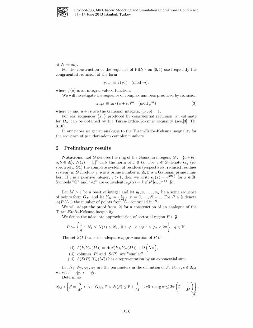
Proceedings, 6th Chaotic Modeling and Simulation International Conference
11 - 14 June 2013 Istanbul, Turkey
at N →∞).For the construction of the sequence of PRN’s on [0, 1) use frequently the
congruential recursion of the form
yn+1 ≡ f(yn) (mod m),
where f(u) is an integral-valued function.We will investigate the sequence of complex numbers produced by recursion
zn+1 ≡ z0 · (u+ iv)m (mod pm) (3)
where z0 and u+ iv are the Gaussian integers, (z0, p) = 1.For real sequences xn produced by congruential recursion, an estimate
for DN can be obtained by the Turan-Erdos-Koksma inequality (see,[3], Th.3.10).
In our paper we get an analogue to the Turan-Erdos-Koksma inequality forthe sequence of pseudorandom complex numbers.
2 Preliminary results
Notations. Let G denotes the ring of the Gaussian integers, G := a+ bi :a, b ∈ Z; N(z) = |z|2 calls the norm of z ∈ G. For γ ∈ G denote Gγ (re-spectively, G∗γ) the complete system of residues (respectively, reduced residuessystem) in G modulo γ; p is a prime number in Z; p is a Gaussian prime num-ber. If q is a positive integer, q > 1, then we write eq(x) = e2πi
xq for x ∈ R.
Symbols ”O” and ”” are equivalent; νp(α) = k if pk|α, pk+1 6 |α.
Let M > 1 be a positive integer and let y1, y2, . . . , yN be a some sequenceof points form GM and let YM =
ynM
, n = 0, . . . , N − 1. For P ∈ F denote
A(P, YM ) the number of points from YM contained in P .We will adapt the proof from [2] for a construction of an analogue of the
Turan-Erdos-Koksma inequality.We define the adequate approximation of sectorial region P ∈ F,
P :=
z
q: N1 ≤ N(z) ≤ N2, 0 ≤ ϕ1 < arg z ≤ ϕ2 < 2π
, q ∈ N.
The set S(P ) calls the adequate approximation of P if
(i) A(P, YN (M)) = A(S(P ), YN (M)) +O(N
12
),
(ii) volumes |P | and |S(P )| are ”similar”,(iii) A(S(P ), YN (M)) has a representation by an exponential sum.
Let N1, N2, ϕ1, ϕ2 are the parameters in the definition of P . For r, s ∈ ZMwe set r = r
M , s = sM .
Determine
Sr,s :
β =
α
M: α ∈ GM , r < N(β) ≤ r +
1
M, 2πs < argα ≤ 2π
(s+
1
M
).
(4)
548

Proceedings, 6th Chaotic Modeling and Simulation International Conference
11 - 14 June 2013 Istanbul, Turkey
Put
S(P ) := ∪r,s
Sr,s⊂P
Sr,s.
It is obvious that S(P ) = P (N1, N2, ψ1, ψ2), where
N1 = min a
M, a ∈ ZM : N1 ≤
a
M
N2 = min
b
M, b ∈ ZM : N2 ≤
b
M
ψ1 = min
2πa
M, a ∈ ZM : ψ1 ≤
2πa
M
ψ2 = min
2πb
M, b ∈ ZM : ψ2 ≤
2πb
M
We proved the following analogue of the Turan-Erdos-Koksma inequality (see,[3])
Theorem 1. Let M > 1 be integer. Then for any sequence yn, yn ∈ GM ,the discrepancy DN of points
ynM
satisfies to inequality
DN ≤ 2
(1−
(1− 2π
M
)2)
+
+1
M
∑γ∈GMγ 6=0
min
(1
| sinπ<γ|,
1
| sinπ=γ|
)1
N
(|SN |+O
(N
12
)),
where SN =N−1∑n=0
eM (<(γyn)).
Proof. By an analogue with the work[2] we infer
RN (S(P )) :=A(S(P ))
N− |S(P )| = 1
N
N−1∑n=0
χS(P )(xn)− |S(P )|, (5)
where xn = ynM , χ∆ is the characteristic function of the set ∆.
By the equality
χSr,s(x) =∑
α∈Sr,s
1
M2
∑γ∈GM
eM (γ(α− x))
we get
|RN (S(P ))| ≤
≤∑
0 6=γ∈GM
1M2
∣∣∣∣∣ ∑z(r,s)∈Sr,s
eM (−<(γz(r, s)))
∣∣∣∣∣ ·∣∣∣∣ 1N N−1∑
n=0eM (<(γyn))
∣∣∣∣ , (6)
549

Proceedings, 6th Chaotic Modeling and Simulation International Conference
11 - 14 June 2013 Istanbul, Turkey
where z(r, s) is the complex number such that
N(z(r, s)) =r
M, arg z(r, s) =
2πs
M.
In order to calculate the first inner sum over Sr,s one needs an estimate ofthe sum ∑
M=
∑N1<N(ω)≤N2
ϕ1<argω≤ϕ2
eM (<(γω)), (0 6= γ ∈ GM ). (7)
The sum∑M can be considered as a sum of coefficients of Dirichlet series
for the Hecke Z-function over the Gaussian field Q(i):
Zm(s, δ0, δ1) =∑
06=ω∈G
e2πi<(ωδ1)
N(ω + δ0)se4mi argω, (<s > 1).
Putting δ0 = 0, δ1 = γM , we obtain for any T > 1 by a standard way the
following estimates:
∑N(ω)≤X
eM (γω) = (ϕ2 − ϕ1)∑
)N(ω) ≤ xeM (γω) +O
1
T
∑N(ω)≤x
1
+
+O
(ϕ2 − ϕ1)
T∑m=1
∣∣∣∣∣∣∑
N(ω)≤x
eM (γω)e4mi argω
∣∣∣∣∣∣ .
(8)
∑N(ω)≤x
eM (γω)e4mi argω εx
12+ε
M14
+M12 (|m|+ 3)1+ε (9)
(for the details, see Chapter 2 of [1], for example).Next, we have a simple analogue of the estimate of linear exponential sum
over G ∣∣∣∣∣ ∑N1<N(ω)≤N2
22πi<(αω)
∣∣∣∣∣ ≤≤ (N2 −N1)
12 min
((N2 −N1)
12 , 1| sinπ<α| ,
1| sinπ=α|
).
(10)
Now by (4)-(9), putting T = x23 and taking unto account that |P | =
ϕ2−ϕ1
2 (N2 −N1), we obtain our assertion. ut
3 Sequence of PRN’s produced by the cyclic group En.
Let p ≡ 3 (mod 4) be a prime integer. Consider the set of the classes of residue(mod pn) over G, such that for every α ∈ En we have N(α) ≡ ±1 (mod pn).Respectively a convolution of multiplication the set En forms a group. It iswell known that a regular generative element of En is a generative element forany E`, ` = 1, 2, . . . , n. Moreover, |En| = 2(p + 1)pn−1 (|En| is the number ofelements in En).
550

Proceedings, 6th Chaotic Modeling and Simulation International Conference
11 - 14 June 2013 Istanbul, Turkey
We fix the generative element of En and let some z0 ∈ Gn, (N(z0), p) = 1.We call z0 an initial value for the sequence zm, where zm = z0(u + iv)m,m = 0, 1, . . . , N − 1.
Lemma 1. ([4], pp.232-233)Let p ≡ 3 (mod 4), n > 3, and let u + iv is a generative element of the
group En. Then for every 0 ≤ ` ≤ pn−2, 0 ≤ k < 2(p+ 1), we have
(u+ iv)2(p+1)p`+k ≡ A(`, k) + iB(`, k) (mod pn),
where
A(`, k) ≡ A0(k) +A1(k)`+ · · ·+An−1(k)`n−1 (mod pn),
B(`, k) ≡ B0(k) +B1(k)`+ · · ·+Bn−1(k)`n−1 (mod pn).
Moreover,
Aj(k) = Aju(k)−Bjv(k), Bj(k) = Ajv(k) +Bju(k), j = 0, 1, . . . , n− 1;
A0 ≡ 1 (mod p), B0 ≡ 0 (mod p);
A1 ≡ 0 (mod p3), A2 = p2A′2, (A′2, p) = 1;
B1 = pB′1, (B′1, p) = 1, B2 ≡ A3 ≡ B3 ≡ · · · ≡ An−1 ≡ Bn−1 ≡ 0 (mod p3);
u(0) = 1, v(0 = 0), (u(p+ 1), p) = 1, p||v(p+ 1);
(v(k), p) = 1 for k 6= 0, p+ 1.
Corollary 1.
p||A1(k), Aj(k) ≡ 0 (mod p2), j = 2, 3, . . . ; k 6= 0, p+ 1;
p2||A1(0), Aj(0) ≡ 0 (mod p3), j = 2, 3, . . . ;
p2||A1(p+ 1), p2||A2(k), Aj(p+ 1) ≡ 0 (mod p3), j = 3, 4, . . . ;
p2||B2(k) if k 6= 0, p+ 1; B2(k) ≡ 0 (mod p3) else;
Bj(k) ≡ 0 (mod p3), j = 3, 4, . . . ; νp(B1(k)) = 1, k = 0, 1, . . . , 2p+ 1.
Lemma 2. Let α ∈ Gpn , α = phα0, (α0, p) = 1, h < n, and let zm = z0(uiv)m
(mod pn), m = 0, 1, . . . , 2(p+ 1)pn−1 − 1.Then ∣∣∣∣∣∣
N−1∑j=0
epn−1(<(αzj))
∣∣∣∣∣∣ ≤ 2pn−h−r−1
2 ,
where r is determined from (12) and depends on α.
Proof. Let us denote
νp(α) = h, 0 ≤ h < n− 1, α = phα0, (α0, p) = 1;
Mh = 2(p+ 1)pn−1−h.
551

Proceedings, 6th Chaotic Modeling and Simulation International Conference
11 - 14 June 2013 Istanbul, Turkey
Then we have∣∣∣∣∣M0−1∑m=0
epn−h−1(<(α0zm))
∣∣∣∣∣ = p2h
∣∣∣∣∣Mh−1∑m=0
epn−h−1(<(α0zm))
∣∣∣∣∣ =
= p2h
∣∣∣∣∣∣2p+1∑k=0
pn−h−1−1∑`=0
epn−h−1(aAk(`)− bBk(`))
∣∣∣∣∣∣ .(11)
For every k = 0, 1, . . . , 2p+ 1, we consider the polynomial
aAk(`)− bBk(`) =
n−1∑j=0
cj(k)`j ,
where
cj(k) = (aAj − bBj)u(k) + (bAj − aBj)v(k), j = 0, 1, . . . , n− 1.
In particular,
c1(k) = (aA1 − bB1)u(k) + (bA1 − aB1)v(k) =
= (au(k) + bv(k))A1 − (bu(k)− av(k))B1,
c2(k) = (aA2 − bB2)u(k) + (bA2 − aB2)v(k) =
= (au(k) + bv(k))A2 − (bu(k)− av(k))B2.
(12)
We see that for all values of k = 0, 1, . . . , 2p+ 1
νp(A1(k)) 6= νp(B1(k)), νp(A2(k)) 6= νp(B2(k)).
Now if for given α0 and k the inequality
νp(c1(k)) ≥ νp(c2(k)) = r (13)
holds, then the inner sum over ` in (10) can be estimated as pn−h+r−1
2 (suchsum by consequent slope leads to the Gaussian sum).
In other cases (i.e., νp(c1(k)) < νp(c2(k))) this sum is vanishes.Hence, from (10)-(12) we infer the assertion of lemma. ut
Lastly we prove the main result
Theorem 2. Let the sequence zn is generated by the recursion
zm+1 ≡ zm(u+ iv) (mod pn),
where z0 ∈ Gpm , u + iv is a generative element of the group En of classes ofresidue modulo pn with the norms that ≡ 1 (mod pn). Then the discrepancy of
the pointszmpm
, m = 0, 1, . . . , N − 1, N ≤ 2(p+ 1)pn−1 satisfies the following
inequality
DN ≤ 2
(1−
(1− 2π
pn
)2)
+N−1pn2 log pn.
552

Proceedings, 6th Chaotic Modeling and Simulation International Conference
11 - 14 June 2013 Istanbul, Turkey
Proof. Indeed, for every h, 0 ≤ h ≤ n− 1 there is at most O(pn−h−r) numbersα0, α0 ∈ Gpn−h for which νp(c1(k)) ≥ νp(c2(k)) = r, where c1(k), c2(k) deter-mined by (11).
Now, by Lemma 2 and Theorem 1 we immediately obtain the proof oftheorem. ut
Theorem 1 makes possible to prove that the sequence of complex numbers znproduced by the recursion
zn+1 ≡ αz−1n + β + γzn (mod pn),
α, β, γ, z0 ∈ G, (α, p) = (z0, p) = 1, β ≡ γ ≡ 0 (mod p), passes s-dimensionaltest on equidistribution and unpredictability.
References
1.R. C. Baker. Diophantine Inequalities. LMS Monographs (New Series),v.1(Clarendon Press, Oxford), 1986.
2.P. Hellekalen. General discrepancy estimates the Walsh function system. ActaArith., 67:209-218, 1994.
3.H. Niederreiter. Random Number Generation and Quasi-Monte Carlo Methods,SIAM, Philadelphia, 1992.
4.S. Varbanets. The Norm Kloosterman Sums Over Z[i]. Analytic and ProbabilisticMethods in Number Theory, Proc. Forth. International Conference in Honour ofJ. Kubilius, Palanga, Lithuania, 25-29 Semtember, 213-224, 2006.
553

Proceedings, 6th Chaotic Modeling and Simulation International Conference
11 - 14 June 2013 Istanbul, Turkey
554
Proceedings, 6th Chaotic Modeling and Simulation International Conference
11 - 14 June 2013 Istanbul, Turkey
Linear-inversive congruential pseudo-randomnumbers with prime power modulus
Vadim Rudetskiy1, Tran The Vinh2, Pavel Varbanets3, and Sergey Varbanets4
1 I. I. Mechnikov Odessa National University, 65026 Odessa, Ukraine(E-mail: [email protected])
2 I. I. Mechnikov Odessa National University, 65026 Odessa, Ukraine(E-mail: [email protected])
3 I. I. Mechnikov Odessa National University, 65026 Odessa, Ukraine(E-mail: [email protected])
4 I. I. Mechnikov Odessa National University, 65026 Odessa, Ukraine(E-mail: [email protected])
Abstract. Studied the sequence of pseudo-random numbers produced by the linear-inversive congruential generator with the special conditions on the parameters ofgenerator. Obtained the individual and averaged by initial value the estimates ofexponential sums on the sequence of pseudo-random numbers.Keywords: pseudo-random numbers, linear-inversive generator, discrepancy, expo-nential sum.
1 Introduction
The Nonlinear methods for pseudo-random number generation provide rea-sonable equidistribution and statistical independence properties. Unfortunatelya classical standard method of generating the pseudo-random numbers in theinterval [0, 1) by a linear recursion yn+1 ≡ ayn + n (mod m) does not inquirewith this problem.
A particularly promising nonlinear method is the inversive congruentialmethod where nonlinearity is achieved by employing the operation of multi-plicative inversion with a respect to given modulus of a typical representer ofsuch generating is the following congruential recursion
yn+1 ≡ ay−1n + b (mod M), (1)
where u−1 is a multiplicative inverse modM if (u,M) = 1.Usually, modulus M select is equal to an odd prime (see, [1][2],[4]) or an
odd prime power (see,[3],[6],[7],[8]). However, it has a priority of existence forthe linear-inversive congruential generator.
yn+1 ≡ ay−1n + b+ cyn (mod pm). (2)
Example, in [3] it is obtained the condition for which a generated sequenceyn has a period of maximal length for p = 2. In [8] it was studied the gener-ator (2) with (y0, p) = (a, p) = 1, b ≡ c ≡ 0 (mod p) and inferred the conditionwhen yn has a maximal period τ . For normalizing sequence ynpm there is
555

Proceedings, 6th Chaotic Modeling and Simulation International Conference
11 - 14 June 2013 Istanbul, Turkey
obtained a non-trivial estimate of discrepancy DN
(y1pm , . . . ,
yNpm
), N ≤ τ .
The sequence xn, xn = ynpm we call the sequence of pseudo-random num-
bers.In present paper we investigate the linear-inversive generator (2) under con-
ditions a ≡ b ≡ 0 (mod p), (c, p) = 1. Notice that the conditions a ≡ b ≡ 0(mod p), (c, p) = 1 or (a, p) = 1, b ≡ c ≡ 0 (mod p) guarantee an existence ofyn for any value of n if (y0, p) = 1.
W.-S. Chou[1] shows that for for generator (1) the conditions a ≡ 0 (mod p),(b, p) = 1 produce corresponding sequence yn with a period τ = 1. It is notalright for an applications. We will prove that the sequence yn produced by(2) has reasonably large period. As well, we give the description of yn as thepolynomial on n and initial value y0. It makes possible to obtain an acceptableestimate for the discrepancy function DN .
Throughout this paper will be used the following
Notation:
For an integer q > 1 we denote by Zq the residue ring of integersmodulo q.As usual, we denote Z∗q the set of invertible elements of Zq.
The notation eq(x) stands for e2πixq .
For u ∈ Z∗pm we use the notation u−1 if uu−1 ≡ 1 (mod pm).
We write νp(a) = k if pk||a.
2 Auxiliary lemmas and preliminary results
In this section we shall gather some auxiliary results which we will useduring the course of the proof of theorems.
Lemma 1. Let p be a prime and let f(x) ∈ Z[x] be a polynomial of degree n,n ≥ 2,
f(x) = a1x+ a2x2 + a3x
3 + · · ·+ anxn,
where νp(aj) ≥ νp(a2) > 0, j ≥ 3.Then the following estimates∣∣∣∣∣∣
∑x∈Zpm
epm(f(x))
∣∣∣∣∣∣ ≤
0 if νp(a1) < νp(a2),
2pm+νp(a2)
2 if νp(a1) ≥ νp(a2).
hold.
This assertion is a corollary of the estimate of Gauss sum.Let xn is a sequence of numbers from [0, 1). Form the sequence of s-
dimensional points X(s)n = (xn, xn+1, . . . , xn+s−1), n = 1, s, . . . , N . We say
that xn passes the s-dimensional discrepancy test if for every j = 1, 2, . . . , s
the sequence X(j)n has a discrepancy which tends to zero for N →∞.
Consider a point sets Ps from [0, 1)s for which all coordinates of all points are
556

Proceedings, 6th Chaotic Modeling and Simulation International Conference
11 - 14 June 2013 Istanbul, Turkey
rational numbers of the form aq , 0 ≤ a < q. Let us denote C(q) =
(−a2 ,
a2
]∩Z,
C∗(q) = a ∈ C(q)|(a, q) = 1. Let Cs(q) (respectively, C∗s (q)) be the innerproduct of s copies of C(q) (respectively, C∗(q)).
Lemma 2 (Niederreiter,[5]). For an integer M ≥ 2 and y0, . . . , yN−1 ∈ Zs,let P be the point set consisting of the fractional parts M−1y0, . . . , M−1yN−1.Then
DN (P ) ≤ 1−(
1− 1
M
)s+
∑h∈C∗
s (M)
1
r(h,M)
∣∣∣∣∣ 1
N
N−1∑n=0
e
(1
Mh · yn
)∣∣∣∣∣ .From this lemma it is seen that the non-trivial estimates of exponential sums
over the sequence of X(s)n are important for the further investigation we
presented.
Proposition 1. Let yn be the sequence produced by the recursion (2) withthe parameters a ≡ b ≡ 0 (mod p), (c, p) = (y0, p) = 1. There are exist thepolynomial Fk(u, v) ∈ Z[u, v] such that for k ≥ m+ 1 we have
yk ≡ Fk(y0, y−10 ) := A0k +A1ky0 +B1ky
−10 +
+B2ky−20 +B3ky
−30 + · · ·+Bm1ky
−m10 (mod pm),
Bjk ≡ 0 (mod pm0), j ≥ 4, m0 = 2νp(a) + νp(b), m1 ≤[
m
νp(a · b)
],
(3)
where the coefficients Aik, Bjk defined by the following relations (4) and(5).
Proof. By (2) we sequentially infer
y1 ≡ ay−10 + b+ cy0 (mod pm)
y2 ≡a
ay−10 + b+ cy0+ b+ c(ay−10 + b+ cy0) ≡
≡ ac−1y−10
(1− c−1y−10 (b+ ay−10 ) + c−2y−20 (b+ ay−10 )2 + · · ·+
+b+ c(ay−10 + b+ cy0))≡
≡ A0,2 +A1,2y0 +B1,2y−10 +B2,2y
−20 +B3,2y
−30 + · · · ,
where modulo pm0 , m0 = 2νp(a) + νp(b), we have
A0,2 = b(1 + c), A1,2 = c2, B1,2 = a(c+ c−1), B2,2 = −abc−2,B3,2 = ab2c−3, Bj,2 = 0, j = 4, 5, . . . .
Let
yk = A0,k +A1,ky0 +B1,ky−10 +B2,ky
−20 +B3,ky
−30 +B4,ky
−40 + · · · .
Then modulo pm0
yk+1 = (b+ cA0,k) + cA1,ky0 + (cB1,k + aA−11,k)y−10 +
+ (cB2,k − aA0,kA−21,k)y−20 + (cB3,k − aA−21,kB1,k + aA−20,kA
−31,k)y−30 .
557

Proceedings, 6th Chaotic Modeling and Simulation International Conference
11 - 14 June 2013 Istanbul, Turkey
Hence, after simple calculations we deduce
A0,3 = b(1 + c+ c2), A1,3 = c3, B1,3a(c2 + 1 + c−2),
B2,3 = −ab(2c−1 + c−2), B3,3 = ab2c−2 − a2c−2(c+ c−1) + ab2c−6(1 + c)2,
and for k > 3A0,k+1 = b c
k+1−1c−1 , A1,k+1 = ck+1, B1,k+1 = a(c2 + 1) + a(k − 1)c−k,
B2,k+1 =
−abck−3(2c−1 + c−2) + abc−2(k−1) c
[ k+12 ]−1
c−1 if c 6= 1,
3ab+ 2−1abk if c = 1.
(4)
Similarly,B3,k+1 ≡ ac−2(b2g1(k) + ag2(k)) (5)
where g1(k), g2(k) ∈ Z[x], g1(2) = g2(2) = 0. ut
Corollary 1. Let yn be the sequence produced by the recursion (2), more-over, νp(b) < νp(a). Then in the assumptions of Proposition 1 for k ≥ 3, k ≡ z(mod δ), 0 ≤ z ≤ δ − 1, where δ is an index c mod p, we have
yk ≡ y0 + kpνp(u)+1H1(z, y0, y−1) + k2pνp(au)+1H2(z, y0, y
−1)+
k3pνp(au)+2 + · · · (mod pm)
Proof. If c ≡ 1 (mod p) we have for p > 3
ck = (1 + pu)k ≡ 1 + pa1k + pa2k2 + pa3k
3 + · · ·+ pλsasps (mod pm),
where νp(aj) = jνp(u), j = 1, 2, 3, . . .;νp(aj) ≥ 4νp(u), j = 4, 5, . . ..
Hence, in this case we find from Proposition 1
yk ≡ y0 + kpνp(u)+1G1(y0, y−10 ) + k2pνp(au)+1G2(y0, y
−10 )+
+ k3pνp(au)+2G3(k, y0, y−10 ) (mod pm).
(6)
In the case c 6≡ 1 (mod p) we denote through δ an index of c, 1 < δ ≤ p−1,modulo p.
Let k = δ`+ z, 0 ≤ z ≤ δ − 1, ` ≡ kδ−1 + zδ−1 (mod pm)
ck = (1 + pu)` · cz =
(1 + p`u+
`(`− 1)
2p2u2 + · · ·
)cz,
c−k ≡ 1− p`u+
(`+
`(`− 1)
2p2u2 + · · ·
)cz.
And we again obtain the relation a type of (6)
yk ≡ y0 + kpνp(u)+1G′1(z, y0, y−10 ) + k2pνp(au)+1G′2(z, y0, y
−10 )+
k3pνp(au)+2G′3(z, k, y0, y−10 ) (mod pm),
(7)
where Gi, G′i are the polynomials on k with the coefficients depending on y0,
y−10 , z.The corollary is established. ut
558

Proceedings, 6th Chaotic Modeling and Simulation International Conference
11 - 14 June 2013 Istanbul, Turkey
Corollary 2. The period of the sequence yn generated by (2) is equal toτ = pm−νp(b) if νp(b) < νp(a).
Indeed, from (4), (5) Aj,k+3 ≡ Aj,3 (mod pm),Bj,k+3 ≡ Bj,3 (mod pm),j = 0, 1, 2, 3, . . .
if and only if k ≡ 0 (mod pm−νp(b)).
3 Main results
First in this section we prove the Theorems 1-3 on the estimate of exponen-tial sums of the sequences of PRN’s yn generated by recursion (2).
Theorem 1. Let (h1, h2, p) = 1, νp(h1 + h2) = α, νp(h1k + h2`) = β and letyn be produced by (2). The the following estimates
∣∣∣∣∣∣∑
y0∈Z∗pm
epm(h1y` + h2yk)
∣∣∣∣∣∣ ≤
0 if α < β + νp(b),m− α− β > 0,
2pm+β+νp(b)
2 if α ≥ γ + νp(b),m− α− β > 0,
pm−1(p− 1) in otherwise
hold.
Proof. For 0 ≤ k, ` < τ = pm−νp(b) we have for c 6= 1:
h1yk + h2y` = B0 +B1y0 +B−1y−10 +B−2y
−20 + pν0H(y0, y
−10 ),
where
B1 = b
(h1c
k + h2c`
c− 1
),
B−1 = a(h1 − h2)(c2 − 1) + a[(kh1c
k + `h2c`)− (h1c
k + h2c`)],
B−2 = −ab(2c−1 + c−2)(h1ck−1 + h2c
`−1)+
+ abc2h1c
k1 + h2c`1 − (h1c
k2 + h2c`2)
c− 1,
ν0 = min (νp(ab2), νp(a
2)).
Substituting ck and c` by the polynomials on k or ` and applying Lemma 1 wededuce the statement of the theorem. ut
The case c = 1 gives the same result.
Theorem 2. Let a linear-inversive generator (2) generates the sequence ofPRN’s yn. Then for N ≤ τ = pm−νp(b) we have the following bounds∣∣∣∣∣
N−1∑n=0
epm(hyn)
∣∣∣∣∣m if m > νp(bh),
pm+νp(h)
2
(Nτ + log τ
)if νp(bh) < m,
N otherwise.
559
Proceedings, 6th Chaotic Modeling and Simulation International Conference
11 - 14 June 2013 Istanbul, Turkey
This assertion follows from Corollary 1 and Lemma 1.
Theorem 3. Let the sequence yn be generated by (2) with parameters a, b,c, y0, (y0, p) = (c, p) = 1 and νp(a) > νp(b) = α ≥ 1. Then for every h ∈ Z,νp(h) = s, we have
1
ϕ(pm)
∑y0∈Z∗
pm
∣∣∣∣∣N−1∑n=0
epm(hyn)
∣∣∣∣∣ N12 +Np−
m−12 .
In order to prove this theorem it is sufficiently to apply the schema of argumentfrom the proof of theorem 3 in [8].
Now, taking into account that equidistribution and statistical independency(unpredictability) properties of the uniform PRN’s can be analyzed on thediscrepancy of certain point sets in [0, 1)s we state from the Theorems 2 and 3and Lemma 3 the following statement:
Theorem 4. Let yn generated by (2) with (y0, p) = (c, p) = 1, νp(a) >νp(b) ≤ 1. Then for the sequence xn, yn = xn
pm we have
DN (x0, x1, . . . , xN−1) ≤ 1
pm+ 2N−1p
m−νp(b)2
(1
p
(2
πlog pm +
7
5
)2
+ 1
).
Moreover, for almost all y0 ∈ Zpm
DN (y0, x0, x1, . . . , xN−1) ≤ 1
pm+ 3N
12 p−
m−νp(b)4 log pm.
So, the linear-inversive congruential generator (2) produces the sequences ofPRN’s xn that involve the properties of equidistribution and unpredictability.
References
1.W. S. Chou. The period lengths of inversive congruential recursions. Acta Arith.,73(4):325–341, 1995.
2.J. Eichenauer, J. Lehn. A non-linear congruential pseudorandom number genera-tor.Statist. Hefte, 27:315–326, 1986.
3.T. Kato, L.-M. Wu and N. Yanagihara. On a nonlinear congruential pseudorandomnumber generator. Math. of Comp., 65(213):227-233, 1996.
4.H. Niederreiter. Recent trends in random number and random vector generation.Ann. Oper. Res., 31:323–345, 1991.
5.H. Niederreiter. Random Number Generation and Quasi-Monte Carlo Methods.SIAM, Philadelphia,Pa., 1992.
6.H. Niederreiter, I. Shparlinski. Exponential sums and the distribution of inversivecongruential pseudorandom numbers with prime-power modulus. Acta Arith.,90(1):89–98, 2000.
7.P. Varbanets, S. Varbanets. Exponential sums on the sequences of invergive congru-ential psendorandom numbers with prime-power modulus, VoronoI’s Impact onModern Science, Proc. of IV Intern. Conf. on Anal. Number Theory and SpatialTessellations, Kyiv, 4(1):112–130, 2008.
560

Proceedings, 6th Chaotic Modeling and Simulation International Conference
11 - 14 June 2013 Istanbul, Turkey
8.P. Varbanets, S. Varbanets. Generalizations of Inversive Congruential Generator.Analytic and Probabilistic Methods in Number Theory, Proc. Fifth. InternationalConference in Honour of J. Kubilius, Palanga, Lithuania, 04-10 Semtember 2011,17:265-282, 2012.
561

Proceedings, 6th Chaotic Modeling and Simulation International Conference
11 - 14 June 2013 Istanbul, Turkey
562