Simulation of a Dispersive Tsunami due to the 2016 El Salvador–Nicaragua Outer-Rise

Earthquake (Mw 6.9)

YUICHIRO TANIOKA,1 AMILCAR GEOVANNY CABRERA RAMIREZ,2 and YUSUKE YAMANAKA3

Abstract—The 2016 El Salvador–Nicaragua outer-rise earth-

quake (Mw 6.9) generated a small tsunami observed at the ocean

bottom pressure sensor, DART 32411, in the Pacific Ocean off

Central America. The dispersive observed tsunami is well simu-

lated using the linear Boussinesq equations. From the dispersive

character of tsunami waveform, the fault length and width of the

outer-rise event is estimated to be 30 and 15 km, respectively. The

estimated seismic moment of 3.16 9 1019 Nm is the same as the

estimation in the Global CMT catalog. The dispersive character of

the tsunami in the deep ocean caused by the 2016 outer-rise El

Salvador–Nicaragua earthquake could constrain the fault size and

the slip amount or the seismic moment of the event.

Key words: Tsunami numerical simulation, the Boussinesq

equations, outer-rise earthquake.

1. Introduction

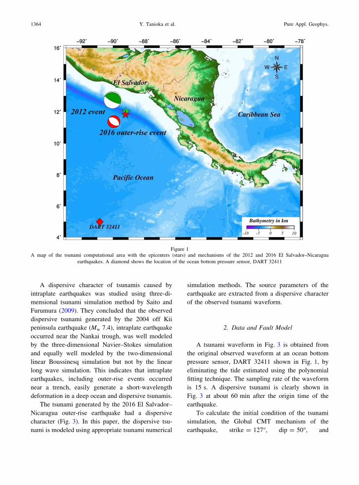
A large earthquake (Mw 6.9) occurred at the outer

rise of the Middle America trench off El Salvador and

Nicaragua on November 24, 2016 (Fig. 1). The

Global CMT solution shows that the mechanism of

the earthquake was a normal fault type

(strike = 127�, dip = 50�, rake = - 89�) with a

centroid depth of 12 km and the seismic moment of

3.16 9 1019 Nm (Mw 6.9). A tsunami warning was

issued along the coast of Nicaragua by the Nicar-

aguan Institute of Territorial Studies (INETER). A

small tsunami was generated by the earthquake and

was detected by only one ocean bottom pressure

sensor, DART 32411 in Fig. 1. No damage was

reported along the coast.

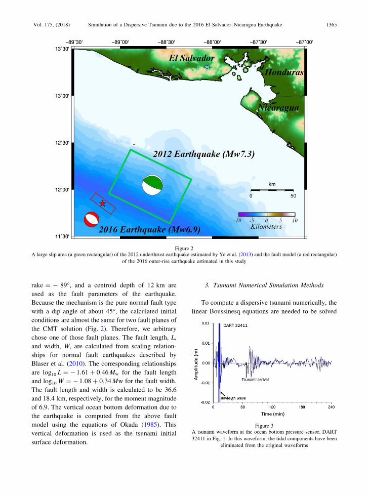
A large underthrust earthquake (Mw 7.3) occurred

on August 27, 2012 near the 2016 earthquake

(Fig. 2). The slip distribution of the 2012 earthquake

was estimated using teleseismic body waves by Ye

et al. (2013) and determined that a large slip occurred

at the plate interface near the trench. Ye et al. (2013)

also estimated a low radiated seismic energy ratio to

the seismic moment (Er/M0) of 1.85 9 10-6 and

suggested that this earthquake was a tsunami earth-

quake. Borrero et al. (2014) also concluded that the

earthquake was a tsunami earthquake by analyzing

the tsunami heights along the coast. Because the

mechanism of the 2016 earthquake occurred in the

outer-rise was a normal fault type, the 2016 event

could be triggered by the 2012 earthquake which

released the stress at the plate interface (Fig. 2).

Previously, Christensen and Ruff (1988) sug-

gested that in the coupled subduction zone, including

Central America, tensional outer-rise earthquakes

occurred after large underthrust earthquakes at the

plate interface. The most recent significant sequence

is the occurrence of the 2007 outer-rise Kurile

earthquake (Mw 8.0) after the 2006 underthrust Kurile

earthquake (Mw 8.3) (Fujii and Satake 2008; Tanioka

et al. 2008). Because the outer-rise event occurred at

shallow depth with a high angle fault, the tsunami

contains much higher frequency component than

those tsunamis caused by typical underthrust earth-

quakes. Toh et al. (2011) shows that the far-field

observed tsunami generated by the 2007 Kurile outer-

rise earthquake had a dispersive character, but the

that generated by the 2006 Kurile underthrust earth-

quake did not.

1 Institute of Seismology and Volcanology, Hokkaido

University, N10W8 Kita-ku, Sapporo, Hokkaido 060-0810, Japan.

E-mail: tanioka@sci.hokudai.ac.jp2 Nicaraguan Institute of Territorial Studies, Managua,

Nicaragua.3 Department of Civil Engineering, The University of Tokyo,

Tokyo, Japan.

Pure Appl. Geophys. 175 (2018), 1363–1370

� 2018 The Author(s)

This article is an open access publication

https://doi.org/10.1007/s00024-018-1773-5 Pure and Applied Geophysics

A dispersive character of tsunamis caused by

intraplate earthquakes was studied using three-di-

mensional tsunami simulation method by Saito and

Furumura (2009). They concluded that the observed

dispersive tsunami generated by the 2004 off Kii

peninsula earthquake (Mw 7.4), intraplate earthquake

occurred near the Nankai trough, was well modeled

by the three-dimensional Navier–Stokes simulation

and equally well modeled by the two-dimensional

linear Boussinesq simulation but not by the linear

long wave simulation. This indicates that intraplate

earthquakes, including outer-rise events occurred

near a trench, easily generate a short-wavelength

deformation in a deep ocean and dispersive tsunamis.

The tsunami generated by the 2016 El Salvador–

Nicaragua outer-rise earthquake had a dispersive

character (Fig. 3). In this paper, the dispersive tsu-

nami is modeled using appropriate tsunami numerical

simulation methods. The source parameters of the

earthquake are extracted from a dispersive character

of the observed tsunami waveform.

2. Data and Fault Model

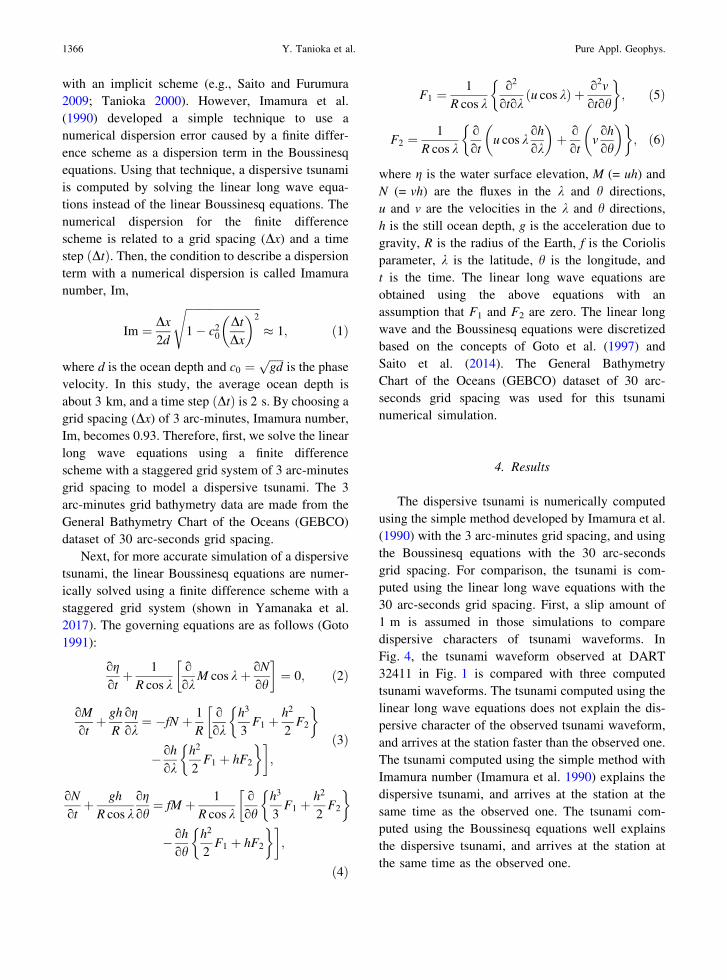
A tsunami waveform in Fig. 3 is obtained from

the original observed waveform at an ocean bottom

pressure sensor, DART 32411 shown in Fig. 1, by

eliminating the tide estimated using the polynomial

fitting technique. The sampling rate of the waveform

is 15 s. A dispersive tsunami is clearly shown in

Fig. 3 at about 60 min after the origin time of the

earthquake.

To calculate the initial condition of the tsunami

simulation, the Global CMT mechanism of the

earthquake, strike = 127�, dip = 50�, and

Figure 1A map of the tsunami computational area with the epicenters (stars) and mechanisms of the 2012 and 2016 El Salvador–Nicaragua

earthquakes. A diamond shows the location of the ocean bottom pressure sensor, DART 32411

1364 Y. Tanioka et al. Pure Appl. Geophys.

rake = - 89�, and a centroid depth of 12 km are

used as the fault parameters of the earthquake.

Because the mechanism is the pure normal fault type

with a dip angle of about 45�, the calculated initial

conditions are almost the same for two fault planes of

the CMT solution (Fig. 2). Therefore, we arbitrary

chose one of those fault planes. The fault length, L,

and width, W, are calculated from scaling relation-

ships for normal fault earthquakes described by

Blaser et al. (2010). The corresponding relationships

are log10 L ¼ � 1:61 þ 0:46Mw for the fault length

and log10 W ¼ � 1:08 þ 0:34Mw for the fault width.

The fault length and width is calculated to be 36.6

and 18.4 km, respectively, for the moment magnitude

of 6.9. The vertical ocean bottom deformation due to

the earthquake is computed from the above fault

model using the equations of Okada (1985). This

vertical deformation is used as the tsunami initial

surface deformation.

3. Tsunami Numerical Simulation Methods

To compute a dispersive tsunami numerically, the

linear Boussinesq equations are needed to be solved

Figure 3A tsunami waveform at the ocean bottom pressure sensor, DART

32411 in Fig. 1. In this waveform, the tidal components have been

eliminated from the original waveforms

Figure 2A large slip area (a green rectangular) of the 2012 underthrust earthquake estimated by Ye et al. (2013) and the fault model (a red rectangular)

of the 2016 outer-rise earthquake estimated in this study

Vol. 175, (2018) Simulation of a Dispersive Tsunami due to the 2016 El Salvador–Nicaragua Earthquake 1365

with an implicit scheme (e.g., Saito and Furumura

2009; Tanioka 2000). However, Imamura et al.

(1990) developed a simple technique to use a

numerical dispersion error caused by a finite differ-

ence scheme as a dispersion term in the Boussinesq

equations. Using that technique, a dispersive tsunami

is computed by solving the linear long wave equa-

tions instead of the linear Boussinesq equations. The

numerical dispersion for the finite difference

scheme is related to a grid spacing (Dx) and a time

step ðDtÞ. Then, the condition to describe a dispersion

term with a numerical dispersion is called Imamura

number, Im,

Im ¼ Dx2d

ffiffiffiffiffiffiffiffiffiffiffiffiffiffiffiffiffiffiffiffiffiffiffiffiffiffiffi

1 � c20

DtDx

� �2s

� 1; ð1Þ

where d is the ocean depth and c0 ¼ffiffiffiffiffi

gdp

is the phase

velocity. In this study, the average ocean depth is

about 3 km, and a time step ðDtÞ is 2 s. By choosing a

grid spacing (Dx) of 3 arc-minutes, Imamura number,

Im, becomes 0.93. Therefore, first, we solve the linear

long wave equations using a finite difference

scheme with a staggered grid system of 3 arc-minutes

grid spacing to model a dispersive tsunami. The 3

arc-minutes grid bathymetry data are made from the

General Bathymetry Chart of the Oceans (GEBCO)

dataset of 30 arc-seconds grid spacing.

Next, for more accurate simulation of a dispersive

tsunami, the linear Boussinesq equations are numer-

ically solved using a finite difference scheme with a

staggered grid system (shown in Yamanaka et al.

2017). The governing equations are as follows (Goto

1991):

ogot

þ 1

R cos ko

okM cos kþ oN

oh

� �

¼ 0; ð2Þ

oM

otþ gh

R

ogok

¼ �fN þ 1

R

o

okh3

3F1 þ

h2

2F2

� ��

� oh

okh2

2F1 þ hF2

� ��

;

ð3Þ

oN

otþ gh

R cos kogoh

¼ fM þ 1

R cos ko

ohh3

3F1 þ

h2

2F2

� ��

� oh

ohh2

2F1 þ hF2

� ��

;

ð4Þ

F1 ¼ 1

R cos ko2

otokðu cos kÞ þ o2v

otoh

� �

; ð5Þ

F2 ¼ 1

R cos ko

otu cos k

oh

ok

� �

þ o

otvoh

oh

� �� �

; ð6Þ

where g is the water surface elevation, M (= uh) and

N (= vh) are the fluxes in the k and h directions,

u and v are the velocities in the k and h directions,

h is the still ocean depth, g is the acceleration due to

gravity, R is the radius of the Earth, f is the Coriolis

parameter, k is the latitude, h is the longitude, and

t is the time. The linear long wave equations are

obtained using the above equations with an

assumption that F1 and F2 are zero. The linear long

wave and the Boussinesq equations were discretized

based on the concepts of Goto et al. (1997) and

Saito et al. (2014). The General Bathymetry

Chart of the Oceans (GEBCO) dataset of 30 arc-

seconds grid spacing was used for this tsunami

numerical simulation.

4. Results

The dispersive tsunami is numerically computed

using the simple method developed by Imamura et al.

(1990) with the 3 arc-minutes grid spacing, and using

the Boussinesq equations with the 30 arc-seconds

grid spacing. For comparison, the tsunami is com-

puted using the linear long wave equations with the

30 arc-seconds grid spacing. First, a slip amount of

1 m is assumed in those simulations to compare

dispersive characters of tsunami waveforms. In

Fig. 4, the tsunami waveform observed at DART

32411 in Fig. 1 is compared with three computed

tsunami waveforms. The tsunami computed using the

linear long wave equations does not explain the dis-

persive character of the observed tsunami waveform,

and arrives at the station faster than the observed one.

The tsunami computed using the simple method with

Imamura number (Imamura et al. 1990) explains the

dispersive tsunami, and arrives at the station at the

same time as the observed one. The tsunami com-

puted using the Boussinesq equations well explains

the dispersive tsunami, and arrives at the station at

the same time as the observed one.

1366 Y. Tanioka et al. Pure Appl. Geophys.

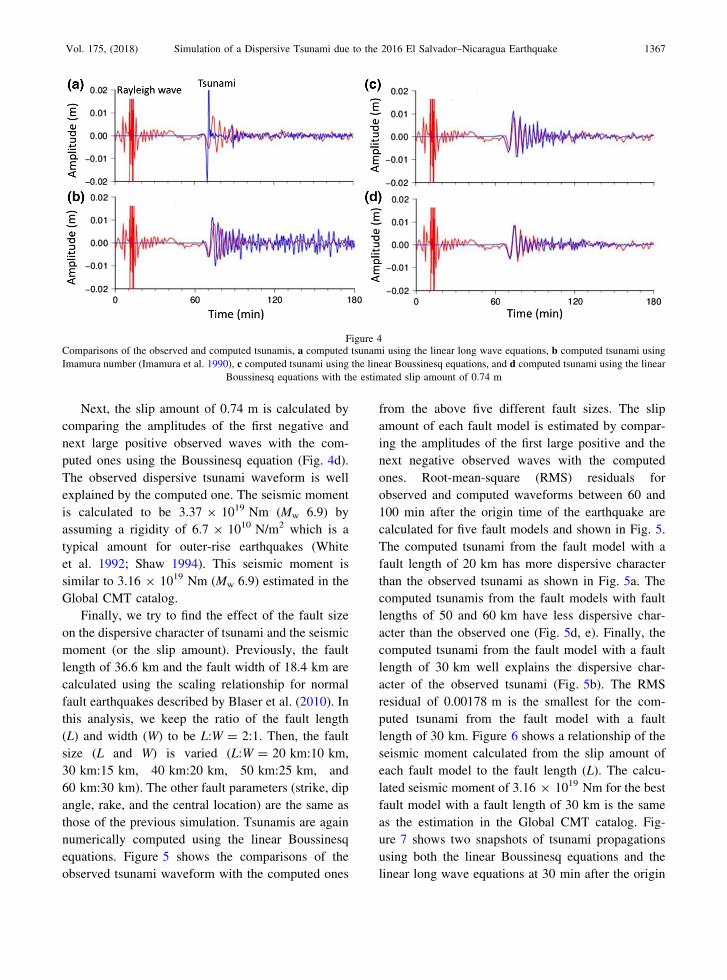
Next, the slip amount of 0.74 m is calculated by

comparing the amplitudes of the first negative and

next large positive observed waves with the com-

puted ones using the Boussinesq equation (Fig. 4d).

The observed dispersive tsunami waveform is well

explained by the computed one. The seismic moment

is calculated to be 3.37 9 1019 Nm (Mw 6.9) by

assuming a rigidity of 6.7 9 1010 N/m2 which is a

typical amount for outer-rise earthquakes (White

et al. 1992; Shaw 1994). This seismic moment is

similar to 3.16 9 1019 Nm (Mw 6.9) estimated in the

Global CMT catalog.

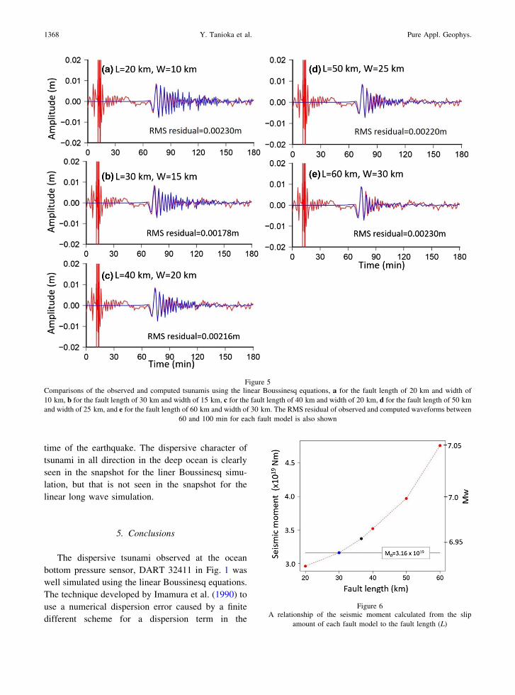
Finally, we try to find the effect of the fault size

on the dispersive character of tsunami and the seismic

moment (or the slip amount). Previously, the fault

length of 36.6 km and the fault width of 18.4 km are

calculated using the scaling relationship for normal

fault earthquakes described by Blaser et al. (2010). In

this analysis, we keep the ratio of the fault length

(L) and width (W) to be L:W = 2:1. Then, the fault

size (L and W) is varied (L:W = 20 km:10 km,

30 km:15 km, 40 km:20 km, 50 km:25 km, and

60 km:30 km). The other fault parameters (strike, dip

angle, rake, and the central location) are the same as

those of the previous simulation. Tsunamis are again

numerically computed using the linear Boussinesq

equations. Figure 5 shows the comparisons of the

observed tsunami waveform with the computed ones

from the above five different fault sizes. The slip

amount of each fault model is estimated by compar-

ing the amplitudes of the first large positive and the

next negative observed waves with the computed

ones. Root-mean-square (RMS) residuals for

observed and computed waveforms between 60 and

100 min after the origin time of the earthquake are

calculated for five fault models and shown in Fig. 5.

The computed tsunami from the fault model with a

fault length of 20 km has more dispersive character

than the observed tsunami as shown in Fig. 5a. The

computed tsunamis from the fault models with fault

lengths of 50 and 60 km have less dispersive char-

acter than the observed one (Fig. 5d, e). Finally, the

computed tsunami from the fault model with a fault

length of 30 km well explains the dispersive char-

acter of the observed tsunami (Fig. 5b). The RMS

residual of 0.00178 m is the smallest for the com-

puted tsunami from the fault model with a fault

length of 30 km. Figure 6 shows a relationship of the

seismic moment calculated from the slip amount of

each fault model to the fault length (L). The calcu-

lated seismic moment of 3.16 9 1019 Nm for the best

fault model with a fault length of 30 km is the same

as the estimation in the Global CMT catalog. Fig-

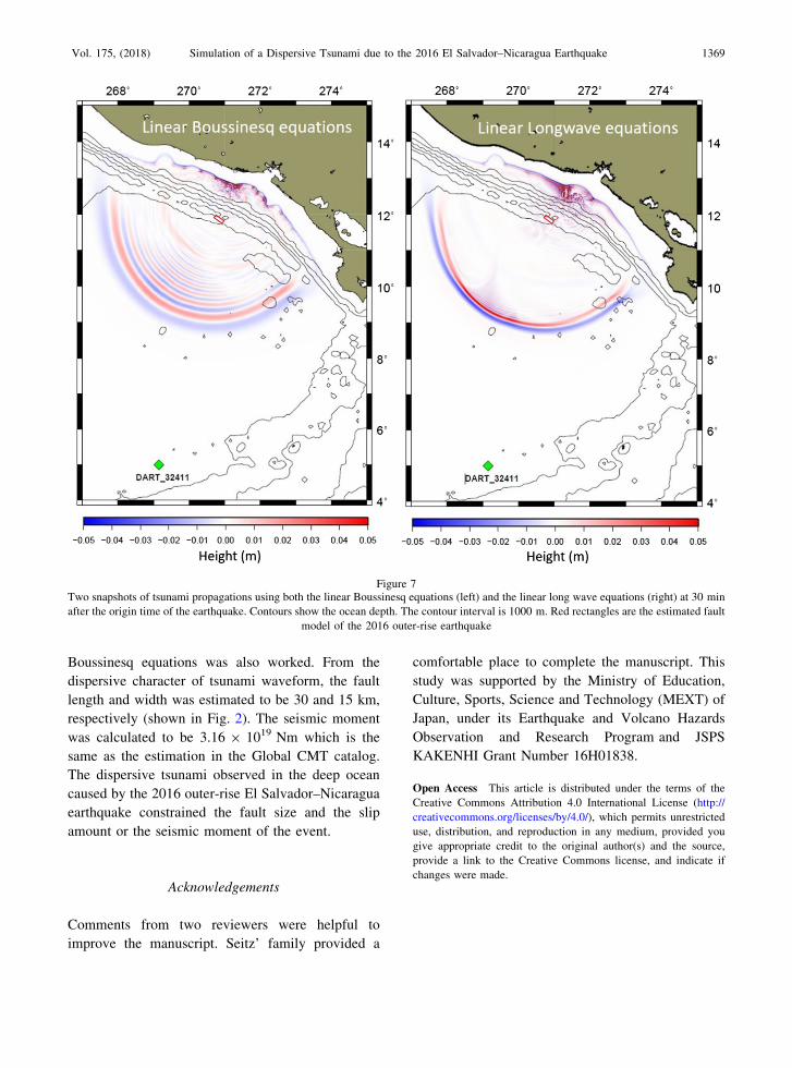
ure 7 shows two snapshots of tsunami propagations

using both the linear Boussinesq equations and the

linear long wave equations at 30 min after the origin

Figure 4Comparisons of the observed and computed tsunamis, a computed tsunami using the linear long wave equations, b computed tsunami using

Imamura number (Imamura et al. 1990), c computed tsunami using the linear Boussinesq equations, and d computed tsunami using the linear

Boussinesq equations with the estimated slip amount of 0.74 m

Vol. 175, (2018) Simulation of a Dispersive Tsunami due to the 2016 El Salvador–Nicaragua Earthquake 1367

time of the earthquake. The dispersive character of

tsunami in all direction in the deep ocean is clearly

seen in the snapshot for the liner Boussinesq simu-

lation, but that is not seen in the snapshot for the

linear long wave simulation.

5. Conclusions

The dispersive tsunami observed at the ocean

bottom pressure sensor, DART 32411 in Fig. 1 was

well simulated using the linear Boussinesq equations.

The technique developed by Imamura et al. (1990) to

use a numerical dispersion error caused by a finite

different scheme for a dispersion term in the

Figure 5Comparisons of the observed and computed tsunamis using the linear Boussinesq equations, a for the fault length of 20 km and width of

10 km, b for the fault length of 30 km and width of 15 km, c for the fault length of 40 km and width of 20 km, d for the fault length of 50 km

and width of 25 km, and e for the fault length of 60 km and width of 30 km. The RMS residual of observed and computed waveforms between

60 and 100 min for each fault model is also shown

Figure 6A relationship of the seismic moment calculated from the slip

amount of each fault model to the fault length (L)

1368 Y. Tanioka et al. Pure Appl. Geophys.

Boussinesq equations was also worked. From the

dispersive character of tsunami waveform, the fault

length and width was estimated to be 30 and 15 km,

respectively (shown in Fig. 2). The seismic moment

was calculated to be 3.16 9 1019 Nm which is the

same as the estimation in the Global CMT catalog.

The dispersive tsunami observed in the deep ocean

caused by the 2016 outer-rise El Salvador–Nicaragua

earthquake constrained the fault size and the slip

amount or the seismic moment of the event.

Acknowledgements

Comments from two reviewers were helpful to

improve the manuscript. Seitz’ family provided a

comfortable place to complete the manuscript. This

study was supported by the Ministry of Education,

Culture, Sports, Science and Technology (MEXT) of

Japan, under its Earthquake and Volcano Hazards

Observation and Research Program and JSPS

KAKENHI Grant Number 16H01838.

Open Access This article is distributed under the terms of the

Creative Commons Attribution 4.0 International License (http://

creativecommons.org/licenses/by/4.0/), which permits unrestricted

use, distribution, and reproduction in any medium, provided you

give appropriate credit to the original author(s) and the source,

provide a link to the Creative Commons license, and indicate if

changes were made.

Figure 7Two snapshots of tsunami propagations using both the linear Boussinesq equations (left) and the linear long wave equations (right) at 30 min

after the origin time of the earthquake. Contours show the ocean depth. The contour interval is 1000 m. Red rectangles are the estimated fault

model of the 2016 outer-rise earthquake

Vol. 175, (2018) Simulation of a Dispersive Tsunami due to the 2016 El Salvador–Nicaragua Earthquake 1369

REFERENCES

Blaser, L., Kruger, F., Ohrnberger, M., & Scherbaum, F. (2010).

Scaling relations of earthquake source parameter estimates with

special focus on subduction environment. Bulletin of the Seis-

mological Society of America, 100(6), 2914–2926.

Borrero, J. C., Kalligeris, N., Lynett, N. P., Fritz, H. M., Newman,

A. V., & Convers, J. A. (2014). Observations and modeling of the

August 27, 2012 earthquake and tsunami affecting El Salvador

and Nicaragua. Pure and Applied Geophysics, 171, 3421–3435.

Christensen, D. H., & Ruff, L. J. (1988). Seismic coupling and

outer rise earthquakes. Journal of Geophysical Research: Solid

Earth, 93(B11), 13421–13444.

Fujii, Y., & Satake, K. (2008). Tsunami sources of the November

2006 and January 2007 great Kuril earthquakes. Bulletin of the

Seismological Society of America, 98(3), 1559–1571.

Goto, C. (1991). Numerical simulation of the trans-oceanic prop-

agation of tsunami. Report of the Port and Harbour Research

Institute, 30, 4–19. (in Japanese).

Goto, C., Ogawa, Y., & Shuto, N. (1997). Numerical method of

tsunami simulation with the leap-frog scheme. IUGG/IOC Time

Project Manuals Guides 35, UNESCO.

Imamura, F., Shuto, N., & Goto, C. (1990). Study on numerical

simulation of the transoceanic propagation of tsunamis—part 2

characteristics of tsunami propagating over the Pacific Ocean,

Zisin. Journal of the Seismological Society of Japan, 43,

389–402.

Okada, Y. (1985). Surface deformation due to shear and tensile

faults in a half-space. Bulletin of the Seismological Society of

America, 75(4), 1135–1154.

Saito, T., & Furumura, T. (2009). Three-dimensional simulation of

tsunami generation and propagation: Application to intraplate

events. Journal of Geophysical Research, 114, B02307. https://

doi.org/10.1029/2007JB005523.

Saito, T., Inazu, D., Miyoshi, T., & Hino, R. (2014). Dispersion and

nonlinear effects in the 2011 Tohoku-Oki earthquake tsunami.

Journal of Geophysical Research: Oceans. https://doi.org/10.

1002/2014jc009971.

Shaw, P. R. (1994). Age variations of oceanic crust Poisson’s ratio:

Inversion and a porosity evolution model. Journal of Geophysi-

cal Research: Solid Earth, 99(B2), 3057–3066.

Tanioka, Y. (2000). Numerical simulation of far-field tsunamis

using the linear Boussinesq equation—the 1998 Papua New

Guinea Tsunami. Papers in Meteorology and Geophysics, 51,

17–25. https://doi.org/10.2467/mripapers.51.17.

Tanioka, Y., Hasegawa, Y., & Kuwayama, T. (2008). Tsunami

waveform analyses of the 2006 underthrust and 2007 outer-rise

Kurile earthquakes. Advances in Geosciences, 14, 129–134.

Toh, H., Satake, K., Hamano, Y., Fujii, Y., & Goto, T. (2011).

Tsunami signal from the 2006 and 2007 Kurile earthquakes

detected at a seafloor geomagnetic observatory. Journal of

Geophysical Research, 116, B02104. https://doi.org/10.1029/

2010JB007873.

White, R. S., McKenzie, D., & O’Nions, R. K. (1992). Oceanic

crustal thickness from seismic measurements and rare earth

element inversions. Journal of Geophysical Research: Solid

Earth, 97(B13), 19683–19715.

Yamanaka, Y., Tanioka, Y., & Shiina, T. (2017). A long source

area of the 1906 Colombia–Ecuador earthquake estimated from

observed tsunami waveforms. Earth, Planets and Space, 69, 163.

https://doi.org/10.1186/s40623-017-0750-z.

Ye, L., Lay, T., & Kanamori, H. (2013). Large earthquake rupture

process variations on the Middle America megathrust. Earth and

Planetary Science Letters, 381, 147–155.

(Received November 24, 2017, revised December 30, 2017, accepted January 4, 2018, Published online January 12, 2018)

1370 Y. Tanioka et al. Pure Appl. Geophys.